appendix - asdlib.org 11: acid–base dissociation constants appendix 12: metal–ligand formation...

1071

Appendix

Appendix 1: NormalityAppendix 2: Propagation of UncertaintyAppendix 3: Single-Sided Normal DistributionAppendix 4: Critical Values for the t-TestAppendix 5: Critical Values for the F-TestAppendix 6: Critical Values for Dixon’s Q-TestAppendix 7: Critical Values for Grubb’s TestAppendix 8: Recommended Primary StandardsAppendix 9: Correcting Mass for the Buoyancy of AirAppendix 10: Solubility ProductsAppendix 11: Acid–Base Dissociation ConstantsAppendix 12: Metal–Ligand Formation ConstantsAppendix 13: Standard Reduction PotentialsAppendix 14: Random Number TableAppendix 15: Polarographic Half-Wave PotentialsAppendix 16: Countercurrent SeparationsAppendix 17: Review of Chemical Kinetics

1072 Analytical Chemistry 2.0

Appendix 1: NormalityNormality expresses concentration in terms of the equivalents of one chemical species reacting stoichio-metrically with another chemical species. Note that this definition makes an equivalent, and thus normality, a function of the chemical reaction. Although a solution of H2SO4 has a single molarity, its normality depends on its reaction.

We define the number of equivalents, n, using a reaction unit, which is the part of a chemical species par-ticipating in the chemical reaction. In a precipitation reaction, for example, the reaction unit is the charge of the cation or anion participating in the reaction; thus, for the reaction

Pb2+(aq) + 2I–(aq) PbI2(s)

n = 2 for Pb2+(aq) and n = 1 for 2I–(aq). In an acid–base reaction, the reaction unit is the number of H+ ions that an acid donates or that a base accepts. For the reaction between sulfuric acid and ammonia

H2SO4(aq) + 2NH3(aq) 2NH4+(aq) + SO4

2–(aq)

n = 2 for H2SO4(aq) because sulfuric acid donates two protons, and n = 1 for NH3(aq) because each ammonia accepts one proton. For a complexation reaction, the reaction unit is the number of electron pairs that the metal accepts or that the ligand donates. In the reaction between Ag+ and NH3

Ag+(aq) + 2NH3(aq) Ag(NH3)2+(aq)

n = 2 for Ag+(aq) because the silver ion accepts two pairs of electrons, and n = 1 for NH3 because each am-monia has one pair of electrons to donate. Finally, in an oxidation–reduction reaction the reaction unit is the number of electrons released by the reducing agent or accepted by the oxidizing agent; thus, for the reaction

2Fe3+(aq) + Sn2+(aq) Sn4+(aq) + 2Fe2+(aq)

n = 1 for Fe3+(aq) and n = 2 for Sn2+(aq). Clearly, determining the number of equivalents for a chemical species requires an understanding of how it reacts.

Normality is the number of equivalent weights, EW, per unit volume. An equivalent weight is the ratio of a chemical species’ formula weight, FW, to the number of its equivalents, n.

EWFW

n=

The following simple relationship exists between normality, N, and molarity, M. N n M= ×

1073Appendices

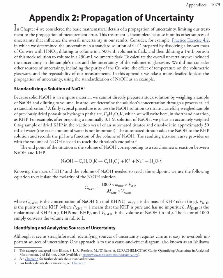
Appendix 2: Propagation of UncertaintyIn Chapter 4 we considered the basic mathematical details of a propagation of uncertainty, limiting our treat-ment to the propagation of measurement error. This treatment is incomplete because it omits other sources of uncertainty that influence the overall uncertainty in our results. Consider, for example, Practice Exercise 4.2, in which we determined the uncertainty in a standard solution of Cu2+ prepared by dissolving a known mass of Cu wire with HNO3, diluting to volume in a 500-mL volumetric flask, and then diluting a 1-mL portion of this stock solution to volume in a 250-mL volumetric flask. To calculate the overall uncertainty we included the uncertainty in the sample's mass and the uncertainty of the volumetric glassware. We did not consider other sources of uncertainty, including the purity of the Cu wire, the effect of temperature on the volumetric glassware, and the repeatability of our measurements. In this appendix we take a more detailed look at the propagation of uncertainty, using the standardization of NaOH as an example.

Standardizing a Solution of NaOH1

Because solid NaOH is an impure material, we cannot directly prepare a stock solution by weighing a sample of NaOH and diluting to volume. Instead, we determine the solution's concentration through a process called a standardization.2 A fairly typical procedure is to use the NaOH solution to titrate a carefully weighed sample of previously dried potassium hydrogen phthalate, C8H5O4K, which we will write here, in shorthand notation, as KHP. For example, after preparing a nominally 0.1 M solution of NaOH, we place an accurately weighed 0.4-g sample of dried KHP in the reaction vessel of an automated titrator and dissolve it in approximately 50 mL of water (the exact amount of water is not important). The automated titrator adds the NaOH to the KHP solution and records the pH as a function of the volume of NaOH. The resulting titration curve provides us with the volume of NaOH needed to reach the titration's endpoint.3

The end point of the titration is the volume of NaOH corresponding to a stoichiometric reaction between NaOH and KHP.

NaOH C H O K C H O K Na H O8 5 4 8 4 2+ → + + +− + +4 ( )l

Knowing the mass of KHP and the volume of NaOH needed to reach the endpoint, we use the following equation to calculate the molarity of the NaOH solution.

CNaOHKHP KHP

KHP NaOH

=× ××

1000 m PM V

where CNaOH is the concentration of NaOH (in mol KHP/L), mKHP is the mass of KHP taken (in g), PKHP is the purity of the KHP (where PKHP = 1 means that the KHP is pure and has no impurities), MKHP is the molar mass of KHP (in g KHP/mol KHP), and VNaOH is the volume of NaOH (in mL). The factor of 1000 simply converts the volume in mL to L.

Identifying and Analyzing Sources of Uncertainty

Although it seems straightforward, identifying sources of uncertainty requires care as it easy to overlook im-portant sources of uncertainty. One approach is to use a cause-and-effect diagram, also known as an Ishikawa

1 This example is adapted from Ellison, S. L. R.; Rosslein, M.; Williams, A. EURACHEM/CITAC Guide: Quantifying Uncertainty in Analytical Measurement, 2nd Edition, 2000 (available at http://www.measurementuncertainty.org/).

2 See Chapter 5 for further details about standardizations.3 For further details about titrations, see Chapter 9.

http://www.measurementuncertainty.org/


diagram—named for its inventor, Kaoru Ishikawa—or a fish bone diagram. To construct a cause-and-effect diagram, we first draw an arrow pointing to the desired result; this is the diagram's trunk. We then add five main branch lines to the trunk, one for each of the four parameters that determine the concentration of NaOH and one for the method's repeatability. Next we add additional branches to the main branch for each of these five factors, continuing until we account for all potential sources of uncertainty. Figure A2.1 shows the complete cause-and-effect diagram for this analysis.

Before we continue, let's take a closer look at Figure A2.1 to be sure we understand each branch of the diagram. To determine the mass of KHP we make two measurements: taring the balance and weighing the gross sample. Each measurement of mass is subject to a calibration uncertainty. When we calibrate a balance, we are essentially creating a calibration curve of the balance's signal as a function of mass. Any calibration curve is subject to a systematic uncertainty in the y-intercept (bias) and an uncertainty in the slope (linearity). We can ignore the calibration bias because it contributes equally to both mKHP(gross) and mKHP(tare), and because we determine the mass of KHP by difference.

m m mKHP KHP(gross) KHP(tare)= −

The volume of NaOH at the end point has three sources of uncertainty. First, an automated titrator uses a piston to deliver the NaOH to the reaction vessel, which means the volume of NaOH is subject to an un-certainty in the piston's calibration. Second, because a solution's volume varies with temperature, there is an additional source of uncertainty due to any fluctuation in the ambient temperature during the analysis. Finally, there is a bias in the titration's end point if the NaOH reacts with any species other than the KHP.

Repeatability, R, is a measure of how consistently we can repeat the analysis. Each instrument we use—the balance and the automatic titrator—contributes to this uncertainty. In addition, our ability to consistently

Figure A2.1 Cause-and-effect diagram for the standardization of NaOH by titration against KHP. The trunk, shown in black, represents the the concentration of NaOH. The remaining arrows represent the sources of uncertainty that affect CNaOH. Light blue arrows, for example, represent the primary sources of uncertainty affecting CNaOH, and green ar-rows represent secondary sources of uncertainty that affect the primary sources of uncertainty. See the text for additional details.

end point

end point

mKHP (gross)mKHP (tare)CNaOH

PKHP mKHP

mKHP

VNaOH

VNaOH

MKHP

calibration

temperature

R

calibrationcalibration

bias

bias

bias

linearity

linearity

1075Appendices

detect the end point also contributes to repeatability. Finally, there are no additional factors that affect the uncertainty of the KHP's purity or molar mass.

Estimating the Standard Deviation for Measurements

To complete a propagation of uncertainty we must express each measurement’s uncertainty in the same way, usually as a standard deviation. Measuring the standard deviation for each measurement requires time and may not be practical. Fortunately, most manufacture provides a tolerance range for glassware and instruments. A 100-mL volumetric glassware, for example, has a tolerance of ±0.1 mL at a temperature of 20 oC. We can convert a tolerance range to a standard deviation using one of the following three approaches.

Assume a Uniform Distribution. Figure A2.2a shows a uniform distribution between the limits of ±x, in which each result between the limits is equally likely. A uniform distribution is the choice when the manufac-turer provides a tolerance range without specifying a level of confidence and when there is no reason to believe that results near the center of the range are more likely than results at the ends of the range. For a uniform distribution the estimated standard deviation, s, is

sx

=3

This is the most conservative estimate of uncertainty as it gives the largest estimate for the standard deviation.Assume a Triangular Distribution. Figure A2.2b shows a triangular distribution between the limits of ±x, in which the most likely result is at the center of the distribution, decreasing linearly toward each limit. A trian-gular distribution is the choice when the manufacturer provides a tolerance range without specifying a level of confidence and when there is a good reason to believe that results near the center of the range are more likely than results at the ends of the range. For a uniform distribution the estimated standard deviation, s, is

sx

=6

This is a less conservative estimate of uncertainty as, for any value of x, the standard deviation is smaller than that for a uniform distribution.Assume a Normal Distribution. Figure A2.3c shows a normal distribution that extends, as it must, beyond the limits of ±x, and which is centered at the mid-point between –x and x. A normal distribution is the choice when we know the confidence interval for the range. For a normal distribution the estimated standard devia-tion, s, is

sxz

=

where z is 1.96 for a 95% confidence interval and 3.00 for a 99.7% confidence interval.

–x x(a)

–x x(b)

–x x(c)

Figure A2.2 Three possible distributions for estimating the standard deviation from a range: (a) a uniform distribution; (b) a triangular distribution; and (c) a normal distribution.


Completing the Propagation of Uncertainty

Now we are ready to return to our example and determine the uncertainty for the standardization of NaOH. First we establish the uncertainty for each of the five primary sources—the mass of KHP, the volume of NaOH at the end point, the purity of the KHP, the molar mass for KHP, and the titration’s repeatability. Having es-tablished these, we can combine them to arrive at the final uncertainty.Uncertainty in the Mass of KHP. After drying the KHP, we store it in a sealed container to prevent it from readsorbing moisture. To find the mass of KHP we first weigh the container, obtaining a value of 60.5450 g, and then weigh the container after removing a portion of KHP, obtaining a value of 60.1562 g. The mass of KHP, therefore, is 0.3888 g, or 388.8 mg. To find the uncertainty in this mass we examine the balance’s calibration certificate, which indicates that its tolerance for linearity is ±0.15 mg. We will assume a uniform distribution because there is no reason to believe that any result within this range is more likely than any other result. Our estimate of the uncertainty for any single measurement of mass, u(m), is

u m( ).

.= =0 15

30 09

mgmg

Because we determine the mass of KHP by subtracting the container’s final mass from its initial mass, the un-certainty of the mass of KHP u(mKHP), is given by the following propagation of uncertainty.

u m( ) ( . ( . .KHP mg) mg) mg= + =0 09 0 09 0 132 2

Uncertainty in the Volume of NaOH. After placing the sample of KHP in the automatic titrator’s reaction ves-sel and dissolving with water, we complete the titration and find that it takes 18.64 mL of NaOH to reach the end point. To find the uncertainty in this volume we need to consider, as shown in Figure A2.1, three sources of uncertainty: the automatic titrator’s calibration, the ambient temperature, and any bias in determining the end point. To find the uncertainty resulting from the titrator’s calibration we examine the instrument’s certificate, which indicates a range of ±0.03 mL for a 20-mL piston. Because we expect that an effective manufacturing process is more likely to produce a piston that operates near the center of this range than at the extremes, we will as-sume a triangular distribution. Our estimate of the uncertainty due to the calibration, u(Vcal) is

u V( ).

.calmL

mL= =0 03

60 012

To determine the uncertainty due to the lack of temperature control, we draw on our prior work in the lab, which has established a temperature variation of ±3 oC with a confidence level of 95%. To find the uncertainty, we convert the temperature range to a range of volumes using water’s coefficient of expansion

2 1 10 3 18 644 1. .×( )× ±( )× ±− −o oC C mL = 0.012 mL

and then estimate the uncertainty due to temperature, u(Vtemp) as

u V( ).

..temp

mLmL= =

0 0121 96

0 006

1077Appendices

Titrations using NaOH are subject to a bias due to the adsorption of CO2, which can react with OH–, as shown here.

CO OH CO H O22 322( ) ( ) ( ) ( )aq aq aq l+ → +− −

If CO2 is present, the volume of NaOH at the end point includes both the NaOH reacting with the KHP and the NaOH reacting with CO2. Rather than trying to estimate this bias, it is easier to bathe the reaction vessel in a stream of argon, which excludes CO2 from the titrator’s reaction vessel.Adding together the uncertainties for the piston’s calibration and the lab’s temperature fluctuation gives the uncertainty in the volume of NaOH, u(VNaOH) as

u V( ) ( . ( . .NaOH mL) mL) mL= + =0 012 0 006 0 0132 2

Uncertainty in the Purity of KHP. According to the manufacturer, the purity of KHP is 100% ± 0.05%, or 1.0 ± 0.0005. Assuming a rectangular distribution, we report the uncertainty, u(PKHP) as

u P( ).

.KHP = =0 0005

30 00029

Uncertainty in the Molar Mass of KHP. The molar mass of C8H5O4K is 204.2212 g/mol, based on the fol-lowing atomic weights: 12.0107 for carbon, 1.00794 for hydrogen, 15.9994 for oxygen, and 39.0983 for po-tassium. Each of these atomic weights has an quoted uncertainty that we can convert to a standard uncertainty assuming a rectangular distribution, as shown here (the details of the calculations are left to you).

element quoted uncertainty standard uncertaintycarbon ±0.0008 ±0.00046hydrogen ±0.00007 ±0.000040oxygen ±0.0003 ±0.00017potassium ±0.0001 ±0.000058

Adding together the uncertainties gives the uncertainty in the molar mass, u(MKHP), as

u M( ) ( . ) ( . ) ( . )KHP = × + × + ×8 0 00046 5 0 000040 4 0 000172 2 2 ++ =( . ) .0 000058 0 0038 g/mol

Uncertainty in the Titration’s Repeatability. To estimate the uncertainty due to repeatability we complete five titrations, obtaining results for the concentration of NaOH of 0.1021 M, 0.1022 M, 0.1022 M, 0.1021 M, and 0.1021 M. The relative standard deviation, sr, for these titrations is

sr5.477

0.1021=

×=

−100 0005

5

.

If we treat the ideal repeatability as 1.0, then the uncertainty due to repeatability, u(R), is equal to the relative standard deviation, or, in this case, 0.0005.Combining the Uncertainties. Table A2.1 summarizes the five primary sources of uncertainty. As described earlier, we calculate the concentration of NaOH we use the following equation, which is slightly modified to include a term for the titration’s repeatability, which, as described above, has a value of 1.0.


CNaOHKHP KHP

KHP NaOH

=× ××

×1000 m P

M VR

Using the values from Table A2.1, we find that the concentration of NaOH is

CNaOH =× ×

×× =

1000 0 3888 1 0204 2212 18 64

1 0 0 1021. .

. .. . MM

Because the calculation of CNaOH includes only multiplication and division, the uncertainty in the con-centration, u(CNaOH) is given by the following propagation of uncertainty.

u CC

u C( ) ( ).

( . )( .

NaOH

NaOH

NaOH

M= =

0 10210 000130 388

2

880 00029

1 00 0038

204 22120 0

2

2

2

2

2)( . )

( . )( . )

( . )( .

+ + +113

18 640 0005

1 0

2

2

2

2

)( . )

( . )( . )

+

Solving for u(CNaOH) gives its value as ±0.00010 M, which is the final uncertainty for the analysis.

Evaluating the Sources of Uncertainty

Figure A2.3 shows the relative uncertainty in the concentration of NaOH and the relative uncertainties for each of the five contributions to the total uncertainty. Of the contributions, the most important is the volume of NaOH, and it is here to which we should focus our attention if we wish to improve the overall uncertainty for the standardization.

Table A2.1 Values and Uncertainties for the Standardization of NaOHsource value, x uncertainty, u(x)

mKHP mass of KHP 0.3888 g 0.00013 gVNaOH volume of NaOH at end point 18.64 mL 0.013 mLPKHP purity of KHP 1.0 0.00029MKHP molar mass of KHP 204.2212 g/mol 0.0038 g/molR repeatability 1.0 0.0005

0.0000 0.0002 0.0004 0.0006 0.0008 0.0010

mKHP

PKHP

MKHP

VNaOH

R

CNaOH

relative uncertainty

Figure A2.3 Bar graph showing the relative uncertainty in CNaOH, and the relative uncertainty in each of the main factors affecting the overall uncertainty.

1079Appendices

Appendix 3: Single-Sided Normal DistributionThe table in this appendix gives the proportion, P, of the area under a normal distribution curve that lies to the right of a deviation, z

zX

=−µσ

where X is the value for which the deviation is being defined, m is the distribution’s mean value and s is the distribution’s standard deviation. For example, the proportion of the area under a normal distribution to the right of a deviation of 0.04 is 0.4840 (see entry in red in the table), or 48.40% of the total area (see the area shaded blue in the figure to the right). The proportion of the area to the left of the deviation is 1 – P. For a deviation of 0.04, this is 1–0.4840, or 51.60%.

When the deviation is negative—that is, when X is smaller than m—the value of z is negative. In this case, the values in the table give the area to the left of z. For example, if z is –0.04, then 48.40% of the area lies to the left of the deviation (see area shaded green in the figure shown below on the left).

To use the single-sided normal distribution table, sketch the normal distribution curve for your problem and shade the area corresponding to your answer (for example, see the figure shown above on the right, which

4-4 -3 -2 -1 0 1 2 3Deviation (z)

48.40%48.40%

230 240 250 260 270Aspirin (mg)

8.08%0.82%

91.10%

is for Example 4.11). This divides the normal distribution curve into three regions: the area corresponding to your answer (shown in blue), the area to the right of this, and the area to the left of this. Calculate the values of z for the limits of the area corresponding to your answer. Use the table to find the areas to the right and to the left of these deviations. Subtract these values from 100% and, voilà, you have your answer.


z 0.00 0.01 0.02 0.03 0.04 0.05 0.06 0.07 0.08 0.090.0 0.5000 0.4960 0.4920 0.4880 0.4840 0.4801 0.4761 0.4721 0.4681 0.46410.1 0.4602 0.4562 0.4522 0.4483 0.4443 0.4404 0.4365 0.4325 0.4286 0.42470.2 0.4207 0.4168 0.4129 0.4090 0.4502 0.4013 0.3974 0.3396 0.3897 0.38590.3 0.3821 0.3783 0.3745 0.3707 0.3669 0.3632 0.3594 0.3557 0.3520 0.34830.4 0.3446 0.3409 0.3372 0.3336 0.3300 0.3264 0.3228 0.3192 0.3156 0.31210.5 0.3085 0.3050 0.3015 0.2981 0.2946 0.2912 0.2877 0.2843 0.2810 0.27760.6 0.2743 0.2709 0.2676 0.2643 0.2611 0.2578 0.2546 0.2514 0.2483 0.24510.7 0.2420 0.2389 0.2358 0.2327 0.2296 0.2266 0.2236 0.2206 0.2177 0.21480.8 0.2119 0.2090 0.2061 0.2033 0.2005 0.1977 0.1949 0.1922 0.1894 0.18670.9 0.1841 0.1814 0.1788 0.1762 0.1736 0.1711 0.1685 0.1660 0.1635 0.16111.0 0.1587 0.1562 0.1539 0.1515 0.1492 0.1469 0.1446 0.1423 0.1401 0.13791.1 0.1357 0.1335 0.1314 0.1292 0.1271 0.1251 0.1230 0.1210 0.1190 0.11701.2 0.1151 0.1131 0.1112 0.1093 0.1075 0.1056 0.1038 0.1020 0.1003 0.09851.3 0.0968 0.0951 0.0934 0.0918 0.0901 0.0885 0.0869 0.0853 0.0838 0.08231.4 0.0808 0.0793 0.0778 0.0764 0.0749 0.0735 0.0721 0.0708 0.0694 0.06811.5 0.0668 0.0655 0.0643 0.0630 0.0618 0.0606 0.0594 0.0582 0.0571 0.05591.6 0.0548 0.0537 0.0526 0.0516 0.0505 0.0495 0.0485 0.0475 0.0465 0.04551.7 0.0466 0.0436 0.0427 0.0418 0.0409 0.0401 0.0392 0.0384 0.0375 0.03671.8 0.0359 0.0351 0.0344 0.0336 0.0329 0.0322 0.0314 0.0307 0.0301 0.02941.9 0.0287 0.0281 0.0274 0.0268 0.0262 0.0256 0.0250 0.0244 0.0239 0.02332.0 0.0228 0.0222 0.0217 0.0212 0.0207 0.0202 0.0197 0.0192 0.0188 0.01832.1 0.0179 0.0174 0.0170 0.0166 0.0162 0.0158 0.0154 0.0150 0.0146 0.01432.2 0.0139 0.0136 0.0132 0.0129 0.0125 0.0122 0.0119 0.0116 0.0113 0.01102.3 0.0107 0.0104 0.0102 0.00964 0.00914 0.008662.4 0.00820 0.00776 0.00734 0.00695 0.006572.5 0.00621 0.00587 0.00554 0.00523 0.00494

2.6 0.00466 0.00440 0.00415 0.00391 0.003682.7 0.00347 0.00326 0.00307 0.00289 0.00272

2.8 0.00256 0.00240 0.00226 0.00212 0.001992.9 0.00187 0.00175 0.00164 0.00154 0.001443.0 0.001353.1 0.0009683.2 0.0006873.3 0.0004833.4 0.000337

3.5 0.0002333.6 0.0001593.7 0.0001083.8 0.00007233.9 0.00004814.0 0.0000317

1081Appendices

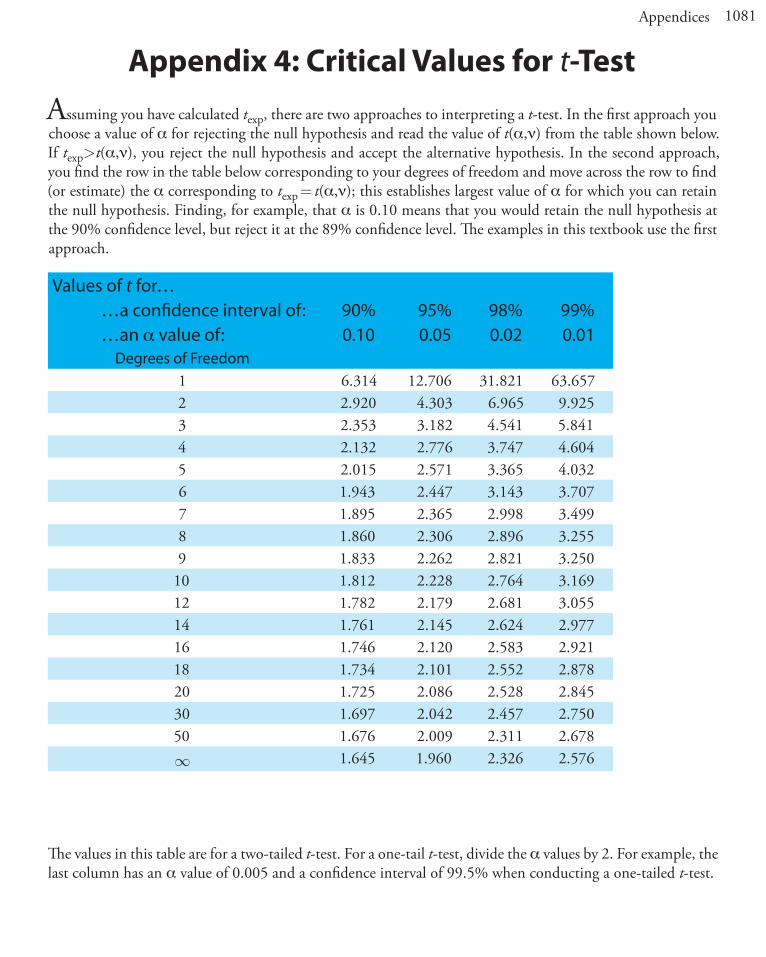
Appendix 4: Critical Values for t-TestAssuming you have calculated texp, there are two approaches to interpreting a t-test. In the first approach you choose a value of a for rejecting the null hypothesis and read the value of t(a,n) from the table shown below. If texp>t(a,n), you reject the null hypothesis and accept the alternative hypothesis. In the second approach, you find the row in the table below corresponding to your degrees of freedom and move across the row to find (or estimate) the a corresponding to texp = t(a,n); this establishes largest value of a for which you can retain the null hypothesis. Finding, for example, that a is 0.10 means that you would retain the null hypothesis at the 90% confidence level, but reject it at the 89% confidence level. The examples in this textbook use the first approach.

Values of t for… …a confidence interval of: 90% 95% 98% 99% …an a value of: 0.10 0.05 0.02 0.01

Degrees of Freedom1 6.314 12.706 31.821 63.6572 2.920 4.303 6.965 9.9253 2.353 3.182 4.541 5.8414 2.132 2.776 3.747 4.6045 2.015 2.571 3.365 4.0326 1.943 2.447 3.143 3.7077 1.895 2.365 2.998 3.4998 1.860 2.306 2.896 3.2559 1.833 2.262 2.821 3.250

10 1.812 2.228 2.764 3.16912 1.782 2.179 2.681 3.05514 1.761 2.145 2.624 2.97716 1.746 2.120 2.583 2.92118 1.734 2.101 2.552 2.87820 1.725 2.086 2.528 2.84530 1.697 2.042 2.457 2.75050 1.676 2.009 2.311 2.678∞ 1.645 1.960 2.326 2.576

The values in this table are for a two-tailed t-test. For a one-tail t-test, divide the a values by 2. For example, the last column has an a value of 0.005 and a confidence interval of 99.5% when conducting a one-tailed t-test.


Appendix 5: Critical Values for the F-TestThe following tables provide values for F(0.05, nnum, ndenom) for one-tailed and for two-tailed F-tests. To use these tables, decide whether the situation calls for a one-tailed or a two-tailed analysis and calculate Fexp

Fssexp =A

B

2

2

where sA2 is greater than sB

2. Compare Fexp to F(0.05, nnum, ndenom) and reject the null hypothesis if Fexp > F(0.05, nnum, ndenom). You may replace s with s if you know the population’s standard deviation.

F(0.05, nnum, ndenom) for a One-Tailed F-Test

denom

num

0

&

o

o

1 2 3 4 5 6 7 8 9 10 15 20 ∞

1 161.4 199.5 215.7 224.6 230.2 234.0 236.8 238.9 240.5 241.9 245.9 248.0 254.32 18.51 19.00 19.16 19.25 19.30 19.33 19.35 19.37 19.38 19.40 19.43 19.45 19.503 10.13 9.552 9.277 9.117 9.013 8.941 8.887 8.845 8.812 8.786 8.703 8.660 8.5264 7.709 6.994 6.591 6.388 6.256 6.163 6.094 6.041 5.999 5.964 5.858 5.803 5.6285 6.608 5.786 5.409 5.192 5.050 4.950 4.876 4.818 4.722 4.753 4.619 4.558 4.3656 5.591 5.143 4.757 4.534 4.387 4.284 4.207 4.147 4.099 4.060 3.938 3.874 3.6697 5.591 4.737 4.347 4.120 3.972 3.866 3.787 3.726 3.677 3.637 3.511 3.445 3.2308 5.318 4.459 4.066 3.838 3.687 3.581 3.500 3.438 3.388 3.347 3.218 3.150 2.9289 5.117 4.256 3.863 3.633 3.482 3.374 3.293 3.230 3.179 3.137 3.006 2.936 2.707

10 4.965 4.103 3.708 3.478 3.326 3.217 3.135 3.072 3.020 2.978 2.845 2.774 2.53811 4.844 3.982 3.587 3.257 3.204 3.095 3.012 2.948 2.896 2.854 2.719 2.646 2.40412 4.747 3.885 3.490 3.259 3.106 2.996 2.913 2.849 2.796 2.753 2.617 2.544 2.29613 4.667 3.806 3.411 3.179 3.025 2.915 2.832 2.767 2.714 2.671 2.533 2.459 2.20614 4.600 3.739 3.344 3.112 2.958 2.848 2.764 2.699 2.646 2.602 2.463 2.388 2.13115 4.534 3.682 3.287 3.056 2.901 2.790 2.707 2.641 2.588 2.544 2.403 2.328 2.06616 4.494 3.634 3.239 3.007 2.852 2.741 2.657 2.591 2.538 2.494 2.352 2.276 2.01017 4.451 3.592 3.197 2.965 2.810 2.699 2.614 2.548 2.494 2.450 2.308 2.230 1.96018 4.414 3.555 3.160 2.928 2.773 2.661 2.577 2.510 2.456 2.412 2.269 2.191 1.91719 4.381 3.552 3.127 2.895 2.740 2.628 2.544 2.477 2.423 2.378 2.234 2.155 1.87820 4,351 3.493 3.098 2.866 2.711 2.599 2.514 2.447 2.393 2.348 2.203 2.124 1.843

∞ 3.842 2.996 2.605 2.372 2.214 2.099 2.010 1.938 1.880 1.831 1.666 1.570 1.000

1083Appendices

F(0.05, nnum, ndenom) for a Two-Tailed F-Test

denom

num

0

&

o

o

1 2 3 4 5 6 7 8 9 10 15 20 ∞

1 647.8 799.5 864.2 899.6 921.8 937.1 948.2 956.7 963.3 968.6 984.9 993.1 10182 38.51 39.00 39.17 39.25 39.30 39.33 39.36 39.37 39.39 39.40 39.43 39.45 39.503 17.44 16.04 15.44 15.10 14.88 14.73 14.62 14.54 14.47 14.42 14.25 14.17 13.904 12.22 10.65 9.979 9.605 9.364 9.197 9.074 8.980 8.905 8.444 8.657 8.560 8.2575 10.01 8.434 7.764 7.388 7.146 6.978 6.853 6.757 6.681 6.619 6.428 6.329 6.0156 8.813 7.260 6.599 6.227 5.988 5.820 5.695 5.600 5.523 5.461 5.269 5.168 4.8947 8.073 6.542 5.890 5.523 5.285 5.119 4.995 4.899 4.823 4.761 4.568 4.467 4.1428 7.571 6.059 5.416 5.053 4.817 4.652 4.529 4.433 4.357 4.259 4.101 3.999 3.6709 7.209 5.715 5.078 4.718 4.484 4.320 4.197 4.102 4.026 3.964 3.769 3.667 3.333

10 6.937 5.456 4.826 4.468 4.236 4.072 3.950 3.855 3.779 3.717 3.522 3.419 3.08011 6.724 5.256 4.630 4.275 4.044 3.881 3.759 3.644 3.588 3.526 3.330 3.226 2.88312 6.544 5.096 4.474 4.121 3.891 3.728 3.607 3.512 3.436 3.374 3.177 3.073 2.72513 6.414 4.965 4.347 3.996 3.767 3.604 3.483 3.388 3.312 3.250 3.053 2.948 2.59614 6.298 4.857 4.242 3.892 3.663 3.501 3.380 3.285 3.209 3.147 2.949 2.844 2.48715 6.200 4.765 4.153 3.804 3.576 3.415 3.293 3.199 3.123 3.060 2.862 2.756 2.39516 6.115 4.687 4.077 3.729 3.502 3.341 3.219 3.125 3.049 2.986 2.788 2.681 2.31617 6.042 4.619 4.011 3.665 3.438 3.277 3.156 3.061 2.985 2.922 2.723 2.616 2.24718 5.978 4.560 3.954 3.608 3.382 3.221 3.100 3.005 2.929 2.866 2.667 2.559 2.18719 5.922 4.508 3.903 3.559 3.333 3.172 3.051 2.956 2.880 2.817 2.617 2.509 2.13320 5.871 4.461 3.859 3.515 3.289 3.128 3.007 2.913 2.837 2.774 2.573 2.464 2.085

∞ 5.024 3.689 3.116 2.786 2.567 2.408 2.288 2.192 2.114 2.048 1.833 1.708 1.000


Appendix 6: Critical Values for Dixon’s Q-TestThe following table provides critical values for Q(a, n), where a is the probability of incorrectly rejecting the suspected outlier and n is the number of samples in the data set. There are several versions of Dixon’s Q-Test, each of which calculates a value for Qij where i is the number of suspected outliers on one end of the data set and j is the number of suspected outliers on the opposite end of the data set. The values given here are for Q10, where

Q Qexp = =−

10

outlier s value nearest value

large

'

sst value smallest value−

The suspected outlier is rejected if Qexp is greater than Q(a, n). For additional information consult Rorabacher, D. B. “Statistical Treatment for Rejection of Deviant Values: Critical Values of Dixon’s ‘Q’ Parameter and Re-lated Subrange Ratios at the 95% confidence Level,” Anal. Chem. 1991, 63, 139–146.

Critical Values for the Q-Test of a Single Outlier (Q10)

n0&a

0.1 0.05 0.04 0.02 0.01

3 0.941 0.970 0.976 0.988 0.9944 0.765 0.829 0.846 0.889 0.9265 0.642 0.710 0.729 0.780 0.8216 0.560 0.625 0.644 0.698 0.7407 0.507 0.568 0.586 0.637 0.6808 0.468 0.526 0.543 0.590 0.6349 0.437 0.493 0.510 0.555 0.598

10 0.412 0.466 0.483 0.527 0.568

1085Appendices

Appendix 7: Critical Values for Grubb’s TestThe following table provides critical values for G(a, n), where a is the probability of incorrectly rejecting the suspected outlier and n is the number of samples in the data set. There are several versions of Grubb’s Test, each of which calculates a value for Gij where i is the number of suspected outliers on one end of the data set and j is the number of suspected outliers on the opposite end of the data set. The values given here are for G10, where

G GX X

sout

exp = =−

10

The suspected outlier is rejected if Gexp is greater than G(a, n).

G(a, n) for Grubb’s Test of a Single Outlier

n0&a

0.05 0.01

3 1.155 1.1554 1.481 1.4965 1.715 1.7646 1.887 1.9737 2.202 2.1398 2.126 2.2749 2.215 2.387

10 2.290 2.48211 2.355 2.56412 2.412 2.63613 2.462 2.69914 2.507 2.75515 2.549 2.755


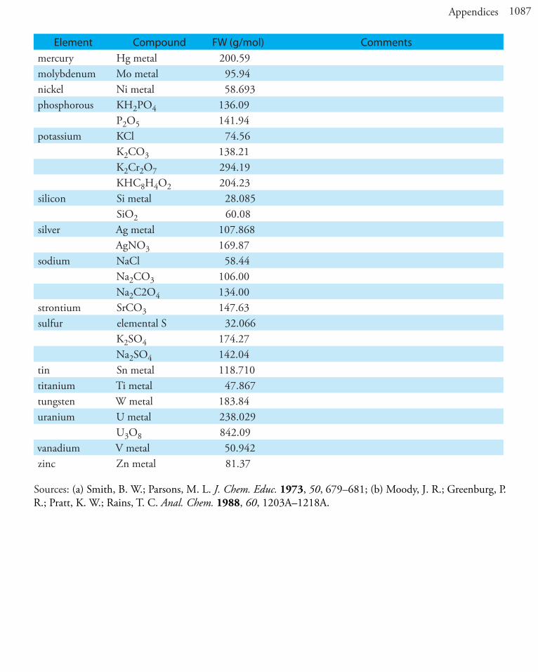
Appendix 8: Recommended Primary StandardsAll compounds should be of the highest available purity. Metals should be cleaned with dilute acid to remove any surface impurities and rinsed with distilled water. Unless otherwise indicated, compounds should be dried to a constant weight at 110 oC. Most of these compounds are soluble in dilute acid (1:1 HCl or 1:1 HNO3), with gentle heating if necessary; some of the compounds are water soluble.

Element Compound FW (g/mol) Commentsaluminum Al metal 26.982antimony Sb metal 121.760

KSbOC4H4O6 324.92 prepared by drying KSbC4H4O6•1/2H2O at 110 oC and storing in a desiccator

arsenic As metal 74.922As2O3 197.84 toxic

barium BaCO3 197.84 dry at 200 oC for 4 hbismuth Bi metal 208.98boron H3BO3 61.83 do not drybromine KBr 119.01cadmium Cd metal 112.411

CdO 128.40calcium CaCO3 100.09cerium Ce metal 140.116

(NH4)2Ce(NO3)4 548.23cesium Cs2CO3 325.82

Cs2SO4 361.87chlorine NaCl 58.44chromium Cr metal 51.996

K2Cr2O7 294.19cobalt Co metal 58.933copper Cu metal 63.546

CuO 79.54fluorine NaF 41.99 do not store solutions in glass containersiodine KI 166.00

KIO3 214.00iron Fe metal 55.845lead Pb metal 207.2lithium Li2CO3 73.89magnesium Mg metal 24.305manganese Mn metal 54.938

1087Appendices

Element Compound FW (g/mol) Commentsmercury Hg metal 200.59molybdenum Mo metal 95.94nickel Ni metal 58.693phosphorous KH2PO4 136.09

P2O5 141.94potassium KCl 74.56

K2CO3 138.21K2Cr2O7 294.19KHC8H4O2 204.23

silicon Si metal 28.085SiO2 60.08

silver Ag metal 107.868AgNO3 169.87

sodium NaCl 58.44Na2CO3 106.00Na2C2O4 134.00

strontium SrCO3 147.63sulfur elemental S 32.066

K2SO4 174.27Na2SO4 142.04

tin Sn metal 118.710titanium Ti metal 47.867tungsten W metal 183.84uranium U metal 238.029

U3O8 842.09vanadium V metal 50.942zinc Zn metal 81.37

Sources: (a) Smith, B. W.; Parsons, M. L. J. Chem. Educ. 1973, 50, 679–681; (b) Moody, J. R.; Greenburg, P. R.; Pratt, K. W.; Rains, T. C. Anal. Chem. 1988, 60, 1203A–1218A.


Appendix 9: Correcting Mass for the Buoyancy of Air

Calibrating a balance does not eliminate all sources of determinate error in the signal. Because of the buoy-ancy of air, an object always weighs less in air than it does in a vacuum. If there is a difference between the object’s density and the density of the weights used to calibrate the balance, then we can make a correction for buoyancy.1 An object’s true weight in vacuo, Wv, is related to its weight in air, Wa, by the equation

.W WD D

11 1

0 0012v ao w

# #= + -f p> H A9.1

where Do is the object’s density, Dw is the density of the calibration weight, and 0.0012 is the density of air under normal laboratory conditions (all densities are in units of g/cm3). The greater the difference between Do and Dw the more serious the error in the object’s measured weight.

The buoyancy correction for a solid is small, and frequently ignored. It may be significant, however, for low density liquids and gases. This is particularly important when calibrating glassware. For example, we can calibrate a volumetric pipet by carefully filling the pipet with water to its calibration mark, dispensing the wa-ter into a tared beaker, and determining the water’s mass. After correcting for the buoyancy of air, we use the water’s density to calculate the volume dispensed by the pipet.

Example

A 10-mL volumetric pipet was calibrated following the procedure just outlined, using a balance calibrated with brass weights having a density of 8.40 g/cm3. At 25 oC the pipet dispensed 9.9736 g of water. What is the actual volume dispensed by the pipet and what is the determinate error in this volume if we ignore the buoyancy correction? At 25 oC the density of water is 0.997 05 g/cm3.

SolutionUsing equation A9.1 the water’s true weight is

Wv = 9 . 9736 g # 1+0 . 99705

1-

8 . 401e o# 0 . 0012> H= 9 . 9842 g

and the actual volume of water dispensed by the pipet is

9 98420 99705

10 014 10 014.

.. .

gg/cm

cm mL3

3= =

If we ignore the buoyancy correction, then we report the pipet’s volume as

9 97360 99705

10 003 10 003.

.. .

gg/cm

cm mL3

3= =

introducing a negative determinate error of -0.11%.

1 Battino, R.; Williamson, A. G. J. Chem. Educ. 1984, 61, 51–52.

1089Appendices

Problems

The following problems will help you in considering the effect of buoyancy on the measurement of mass.

1. In calibrating a 10-mL pipet a measured volume of water was transferred to a tared flask and weighed, yielding a mass of 9.9814 grams. (a) Calculate, with and without correcting for buoyancy, the volume of water delivered by the pipet. Assume that the density of water is 0.99707 g/cm3 and that the density of the weights is 8.40 g/cm3. (b) What are the absolute and relative errors introduced by failing to account for the effect of buoyancy? Is this a significant source of determinate error for the calibration of a pipet? Explain.

2. Repeat the questions in problem 1 for the case where a mass of 0.2500 g is measured for a solid that has a density of 2.50 g/cm3.

3. Is the failure to correct for buoyancy a constant or proportional source of determinate error?

4. What is the minimum density of a substance necessary to keep the buoyancy correction to less than 0.01% when using brass calibration weights with a density of 8.40 g/cm3?


Appendix 10: Solubility ProductsThe following table provides pKsp and Ksp values for selected compounds, organized by the anion. All values are from Martell, A. E.; Smith, R. M. Critical Stability Constants, Vol. 4. Plenum Press: New York, 1976. Un-less otherwise stated, values are for 25 oC and zero ionic strength.

Bromide (Br–) pKsp Ksp

CuBr 8.3 5.×10–9

AgBr 12.30 5.0×10–13

Hg2Br2 22.25 5.6×10–13

HgBr2 (m = 0.5 M) 18.9 1.3×10–19

PbBr2 (m = 4.0 M) 5.68 2.1×10–6

Carbonate (CO32–) pKsp Ksp

MgCO3 7.46 3.5×10–8

CaCO3 (calcite) 8.35 4.5×10–9

CaCO3 (aragonite) 8.22 6.0×10–9

SrCO3 9.03 9.3×10–10

BaCO3 8.30 5.0×10–9

MnCO3 9.30 5.0×10–10

FeCO3 10.68 2.1×10–11

CoCO3 9.98 1.0×10–10

NiCO3 6.87 1.3×10–7

Ag2CO3 11.09 8.1×10–12

Hg2CO3 16.05 8.9×10–17

ZnCO3 10.00 1.0×10–10

CdCO3 13.74 1.8×10–14

PbCO3 13.13 7.4×10–14

Chloride (Cl–) pKsp Ksp

CuCl 6.73 1.9×10–7

AgCl 9.74 1.8×10–10

Hg2Cl2 17.91 1.2×10–18

PbCl2 4.78 2.0×10–19

1091Appendices

Chromate (CrO42–) pKsp Ksp

BaCrO4 9.67 2.1×10–10

CuCrO4 5.44 3.6×10–6

Ag2CrO4 11.92 1.2×10–12

Hg2CrO4 8.70 2.0×10–9

Cyanide (CN–) pKsp Ksp

AgCN 15.66 2.2×10–16

Zn(CN)2 (m = 3.0 M) 15.5 3.×10–16

Hg2(CN)2 39.3 5.×10–40

Ferrocyanide [Fe(CN)64–] pKsp Ksp

Zn2[Fe(CN)6] 15.68 2.1×10–16

Cd2[Fe(CN)6] 17.38 4.2×10–18

Pb2[Fe(CN)6] 18.02 9.5×10–19

Fluoride (F–) pKsp Ksp

MgF2 8.18 6.6×10–9

CaF2 10.41 3.9×10–11

SrF2 8.54 2.9×10–9

BaF2 5.76 1.7×10–6

PbF2 7.44 3.6×10–8

Hydroxide (OH–) pKsp Ksp

Mg(OH)2 11.15 7.1×10–12

Ca(OH)2 5.19 6.5×10–6

Ba(OH)2•8H2O 3.6 3.×10–4

La(OH)3 20.7 2.×10–21

Mn(OH)2 12.8 1.6×10–13

Fe(OH)2 15.1 8.×10–16

Co(OH)2 14.9 1.3×10–15

Ni(OH)2 15.2 6.×10–16

Cu(OH)2 19.32 4.8×10–20

Fe(OH)3 38.8 1.6×10–39


Co(OH)3 (T = 19 oC) 44.5 3.×10–45

Ag2O (+ H2O 2Ag+ + 2OH–) 15.42 3.8×10–16

Cu2O (+ H2O 2Cu+ + 2OH–) 29.4 4.×10–30

Zn(OH)2 (amorphous) 15.52 3.0×10–16

Cd(OH)2 (b) 14.35 4.5×10–15

HgO (red) (+ H2O Hg2+ + 2OH–) 25.44 3.6×10–26

SnO (+ H2O Sn2+ + 2OH–) 26.2 6.×10–27

PbO (yellow) (+ H2O Pb2+ + 2OH–) 15.1 8.×10–16

Al(OH)3 (a) 33.5 3.×10–34

Iodate (IO3–) pKsp Ksp

Ca(IO3)2 6.15 7.1×10–7

Ba(IO3)2 8.81 1.5×10–9

AgIO3 7.51 3.1×10–8

Hg2(IO3)2 17.89 1.3×10–18

Zn(IO3)2 5.41 3.9×10–6

Cd(IO3)2 7.64 2.3×10–8

Pb(IO3)2 12.61 2.5×10–13

Iodide (I–) pKsp Ksp

AgI 16.08 8.3×10–17

Hg2I2 28.33 4.7×10–29

HgI2 (m = 0.5 M) 27.95 1.1×10–28

PbI2 8.10 7.9×10–9

Oxalate (C2O42–) pKsp Ksp

CaC2O4 (m = 0.1 M, T = 20 oC) 7.9 1.3×10–8

BaC2O4 (m = 0.1 M, T = 20 oC) 6.0 1.×10–6

SrC2O4 (m = 0.1 M, T = 20 oC) 6.4 4.×10–7

Phosphate (PO43–) pKsp Ksp

Fe3(PO4)2•8H2O 36.0 1.×10–36

Zn3(PO4)2•4H2O 35.3 5.×10–36

Ag3PO4 17.55 2.8×10–18

1093Appendices

Pb3(PO4)2 (T = 38 oC) 43.55 3.0×10–44

Sulfate (SO42–) pKsp Ksp

CaSO4 4.62 2.4×10–5

SrSO4 6.50 3.2×10–7

BaSO4 9.96 1.1×10–10

Ag2SO4 4.83 1.5×10–5

Hg2SO4 6.13 7.4×10–7

PbSO4 7.79 1.6×10–8

Sulfide (S2–) pKsp Ksp

MnS (green) 13.5 3.×10–14

FeS 18.1 8.×10–19

CoS (b) 25.6 3.×10–26

NiS (g) 26.6 3.×10–27

CuS 36.1 8.×10–37

Cu2S 48.5 3.×10–49

Ag2S 50.1 8.×10–51

ZnS (a) 24.7 2.×10–25

CdS 27.0 1.×10–27

Hg2S (red) 53.3 5.×10–54

PbS 27.5 3.×10–28

Thiocyanate (SCN–) pKsp Ksp

CuSCN (m = 5.0 M) 13.40 4.0×10–14

AgSCN 11.97 1.1×10–12

Hg2(SCN)2 19.52 3.0×10–20

Hg(SCN)2 (m = 1.0 M) 19.56 2.8×10–20


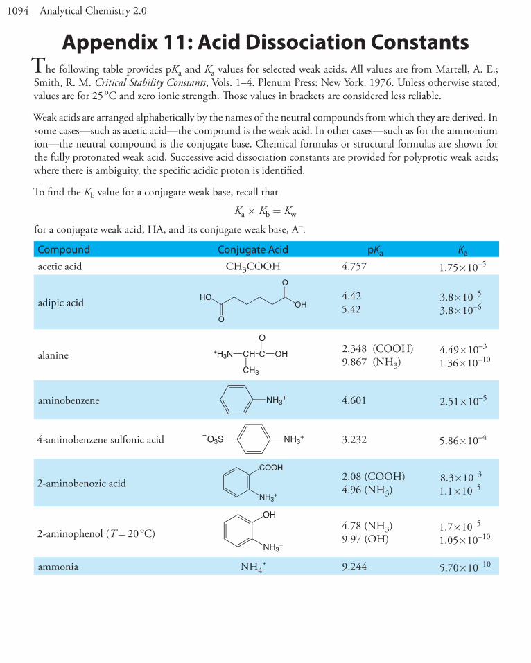
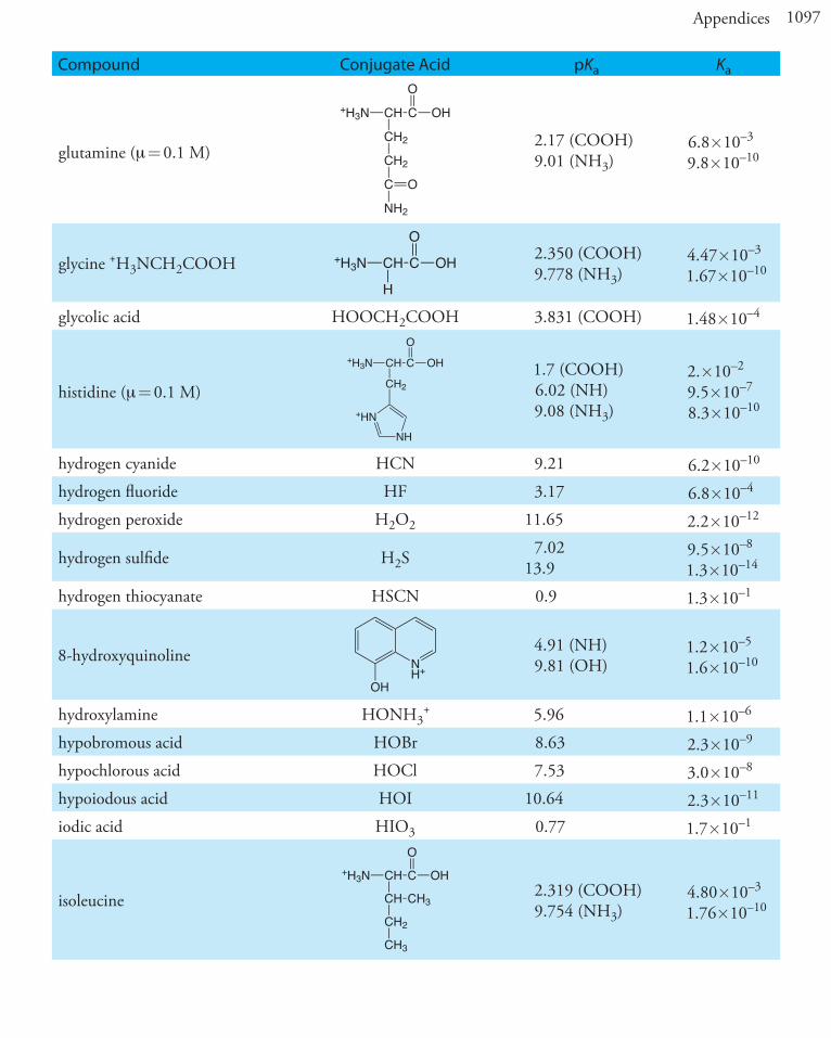
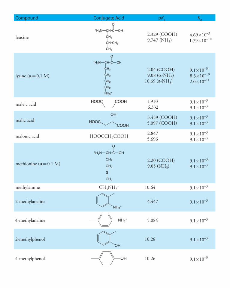
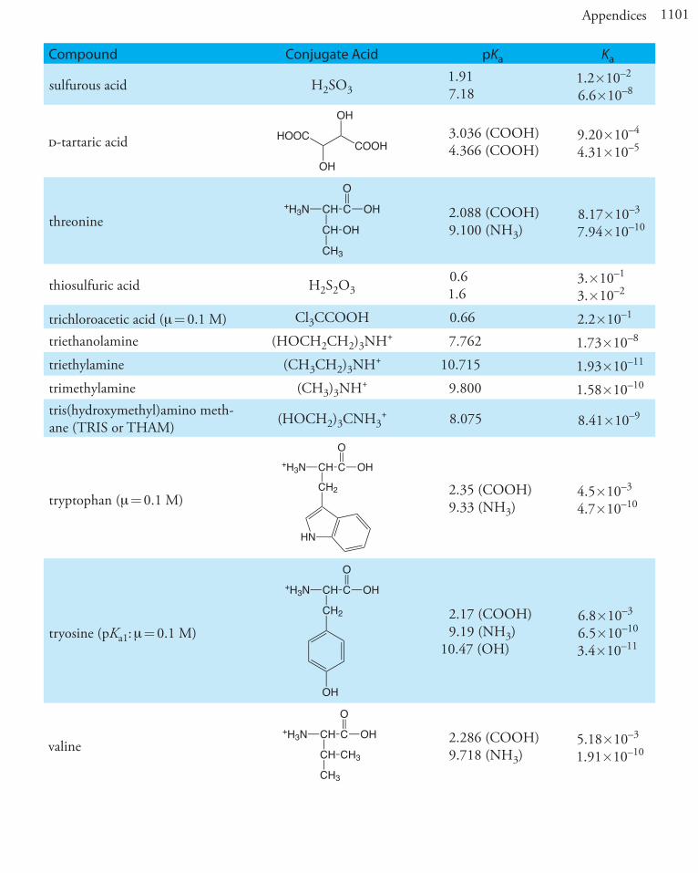
Appendix 11: Acid Dissociation ConstantsThe following table provides pKa and Ka values for selected weak acids. All values are from Martell, A. E.; Smith, R. M. Critical Stability Constants, Vols. 1–4. Plenum Press: New York, 1976. Unless otherwise stated, values are for 25 oC and zero ionic strength. Those values in brackets are considered less reliable.

Weak acids are arranged alphabetically by the names of the neutral compounds from which they are derived. In some cases—such as acetic acid—the compound is the weak acid. In other cases—such as for the ammonium ion—the neutral compound is the conjugate base. Chemical formulas or structural formulas are shown for the fully protonated weak acid. Successive acid dissociation constants are provided for polyprotic weak acids; where there is ambiguity, the specific acidic proton is identified.

To find the Kb value for a conjugate weak base, recall that

Ka × Kb = Kw

for a conjugate weak acid, HA, and its conjugate weak base, A–.

Compound Conjugate Acid pKa Ka

acetic acid CH3COOH 4.757 1.75×10–5

adipic acid HOOH

O

O

4.425.42

3.8×10–5

3.8×10–6

alanine +H3N CH C

CH3

OH

O2.348 (COOH)9.867 (NH3)

4.49×10–3

1.36×10–10

aminobenzene NH3+ 4.601 2.51×10–5

4-aminobenzene sulfonic acid NH3+O3S 3.232 5.86×10–4

2-aminobenozic acidCOOH

NH3+

2.08 (COOH)4.96 (NH3)

8.3×10–3

1.1×10–5

2-aminophenol (T = 20 oC)

OH

NH3+

4.78 (NH3)9.97 (OH)

1.7×10–5

1.05×10–10

ammonia NH4+ 9.244 5.70×10–10

1095Appendices


arginine

+H3N CH C

CH2

OH

O

CH2

CH2

NH

C

NH3+

NH2+

1.823 (COOH)8.991 (NH3)

[12.48] (NH2)

1.50×10–2

1.02×10–9

[3.3×10–13]

arsenic acid H3AsO4

2.246.96

11.50

5.8×10–3

1.1×10–7

3.2×10–12

asparagine (m = 0.1 M)

+H3N CH C

CH2

OH

O

C

NH2

O

2.14 (COOH)8.72 (NH3)

7.2×10–3

1.9×10–9

asparatic acid+H3N CH C

CH2

OH

O

C

OH

O

1.990 (a-COOH)3.900 (b-COOH)

10.002 (NH3)

1.02×10–2

1.26×10–4

9.95×10–11

benzoic acid COOH 4.202 6.28×10–5

benzylamine CH2NH3+ 9.35 4.5×10–10

boric acid (pKa2, pKa3:T = 20 oC) H3BO3

9.236[12.74][13.80]

5.81×10–10

[1.82×10–13][1.58×10–14]

carbonic acid H2CO36.352

10.3294.45×10–7

4.69×10–11

catecholOH

OH

9.4012.8

4.0×10–10

1.6×10–13

chloroacetic acid ClCH2COOH 2.865 1.36×10–3

chromic acid (pKa1:T = 20 oC) H2CrO4-0.2

6.511.63.1×10–7



citric acidCOOH

COOHHOOC

OH

3.128 (COOH)4.761 (COOH)6.396 (COOH)

7.45×10–4

1.73×10–5

4.02×10–7

cupferrron (m = 0.1 M) NNO

OH4.16 6.9×10–5

cysteine+H3N CH C

CH2

OH

O

SH

[1.71] (COOH)8.36 (SH)

10.77 (NH3)

[1.9×10–2]4.4×10–9

1.7×10–11

dichloracetic acid Cl2CHCOOH 1.30 5.0×10–2

diethylamine (CH3CH2)2NH2+ 10.933 1.17×10–11

dimethylamine (CH3)2NH2+ 10.774 1.68×10–11

dimethylglyoximeNOHHON

10.6612.0

2.2×10–11

1.×10–12

ethylamine CH3CH2NH3+ 10.636 2.31×10–11

ethylenediamine +H3NCH2CH2NH3+ 6.848

9.9281.42×10–7

1.18×10–10

ethylenediaminetetraacetic acid (EDTA) (m = 0.1 M)

NH++HN

COOH

COOH

HOOC

HOOC

0.0 (COOH)1.5 (COOH)2.0 (COOH)2.66 (COOH)6.16 (NH)

10.24 (NH)

1.03.2×10–2

1.0×10–2

2.2×10–3

6.9×10–7

5.8×10–11

formic acid HCOOH 3.745 1.80×10–4

fumaric acidCOOH

HOOC

3.0534.494

8.85×10–4

3.21×10–5

glutamic acid

+H3N CH C

CH2

OH

O

CH2

C

OH

O

2.33 (a-COOH)4.42 (l-COOH)9.95 (NH3)

5.9×10–3

3.8×10–5

1.12×10–10

1097Appendices


glutamine (m = 0.1 M)

+H3N CH C

CH2

OH

O

CH2

C

NH2

O

2.17 (COOH)9.01 (NH3)

6.8×10–3

9.8×10–10

glycine +H3NCH2COOH +H3N CH C

H

OH

O2.350 (COOH)9.778 (NH3)

4.47×10–3

1.67×10–10

glycolic acid HOOCH2COOH 3.831 (COOH) 1.48×10–4

histidine (m = 0.1 M)

+H3N CH C

CH2

OH

O

+HNNH

1.7 (COOH)6.02 (NH)9.08 (NH3)

2.×10–2

9.5×10–7

8.3×10–10

hydrogen cyanide HCN 9.21 6.2×10–10

hydrogen fluoride HF 3.17 6.8×10–4

hydrogen peroxide H2O2 11.65 2.2×10–12

hydrogen sulfide H2S 7.0213.9

9.5×10–8

1.3×10–14

hydrogen thiocyanate HSCN 0.9 1.3×10–1

8-hydroxyquinoline NH+

OH

4.91 (NH)9.81 (OH)

1.2×10–5

1.6×10–10

hydroxylamine HONH3+ 5.96 1.1×10–6

hypobromous acid HOBr 8.63 2.3×10–9

hypochlorous acid HOCl 7.53 3.0×10–8

hypoiodous acid HOI 10.64 2.3×10–11

iodic acid HIO3 0.77 1.7×10–1

isoleucine

+H3N CH C

CH

OH

O

CH3

CH2

CH3

2.319 (COOH)9.754 (NH3)

4.80×10–3

1.76×10–10


leucine

+H3N CH C

CH2

OH

O

CH CH3

CH3

2.329 (COOH)9.747 (NH3)

4.69×10–3

1.79×10–10

lysine (m = 0.1 M)

+H3N CH C

CH2

OH

O

CH2

CH2

CH2

NH3+

2.04 (COOH)9.08 (a-NH3)

10.69 (e-NH3)

9.1×10–3

8.3×10–10

2.0×10–11

maleic acid COOHHOOC 1.9106.332

9.1×10–3

9.1×10–3

malic acidOH

COOHHOOC

3.459 (COOH)5.097 (COOH)

9.1×10–3

9.1×10–3

malonic acid HOOCCH2COOH 2.8475.696

9.1×10–3

9.1×10–3

methionine (m = 0.1 M)

+H3N CH C

CH2

OH

O

CH2

S

CH3

2.20 (COOH)9.05 (NH3)

9.1×10–3

9.1×10–3

methylamine CH3NH3+ 10.64 9.1×10–3

2-methylanalineNH3

+4.447 9.1×10–3

4-methylanaline NH3+ 5.084 9.1×10–3

2-methylphenolOH

10.28 9.1×10–3

4-methylphenol OH 10.26 9.1×10–3

1099Appendices


nitrilotriacetic acid (T = 20 oC)(pKa1: m = 0.1 m) NH+

COOH

COOH

HOOC

1.1 (COOH)1.650 (COOH)2.940 (COOH)

10.334 (NH3)

9.1×10–3

9.1×10–3

9.1×10–3

9.1×10–3

2-nitrobenzoic acid

COOH

NO2

2.179 9.1×10–3

3-nitrobenzoic acid

COOH

NO2

3.449 9.1×10–3

4-nitrobenzoic acid COOHO2N 3.442 3.61×10–4

2-nitrophenolOH

NO2

7.21 6.2×10–8

3-nitrophenol

OH

NO2

8.39 4.1×10–9

4-nitrophenol OHO2N 7.15 7.1×10–8

nitrous acid HNO2 3.15 7.1×10–4

oxalic acid H2C2O41.2524.266

5.60×10–2

5.42×10–5

1,10-phenanthroline

NH+ N

4.86 1.38×10–5

phenol OH 9.98 1.05×10–10



phenylalanine

+H3N CH C

CH2

OH

O

2.20 (COOH)9.31 (NH3)

6.3×10–3

4.9×10–10

phosphoric acid H3PO4

2.1487.199

12.35

7.11×10–3

6.32×10–8

4.5×10–13

phthalic acid

COOH

COOH

2.9505.408

1.12×10–3

3.91×10–6

piperdine NH2+ 11.123 7.53×10–12

prolineNH2

+

COOH 1.952 (COOH)10.640 (NH)

1.12×10–2

2.29×10–11

propanoic acid CH3CH2COOH 4.874 1.34×10–5

propylamine CH3CH2CH2NH3+ 10.566 2.72×10–11

pryidine NH+ 5.229 5.90×10–6

resorcinol

OH

OH

9.3011.06

5.0×10–10

8.7×10–12

salicylic acidCOOH

OH

2.97 (COOH)13.74 (OH)

1.1×10–3

1.8×10–14

serine+H3N CH C

CH2

OH

O

OH

2.187 (COOH)9.209 (NH3)

6.50×10–3

6.18×10–10

succinic acid HOOCCOOH

4.2075.636

6.21×10–5

2.31×10–6

sulfuric acid H2SO4strong

1.99—

1.0×10–2

1101Appendices


sulfurous acid H2SO31.917.18

1.2×10–2

6.6×10–8

d-tartaric acid HOOCCOOH

OH

OH

3.036 (COOH)4.366 (COOH)

9.20×10–4

4.31×10–5

threonine+H3N CH C

CH

OH

O

OH

CH3

2.088 (COOH)9.100 (NH3)

8.17×10–3

7.94×10–10

thiosulfuric acid H2S2O30.61.6

3.×10–1

3.×10–2

trichloroacetic acid (m = 0.1 M) Cl3CCOOH 0.66 2.2×10–1

triethanolamine (HOCH2CH2)3NH+ 7.762 1.73×10–8

triethylamine (CH3CH2)3NH+ 10.715 1.93×10–11

trimethylamine (CH3)3NH+ 9.800 1.58×10–10

tris(hydroxymethyl)amino meth-ane (TRIS or THAM) (HOCH2)3CNH3

+ 8.075 8.41×10–9

tryptophan (m = 0.1 M)

+H3N CH C

CH2

OH

O

HN

2.35 (COOH)9.33 (NH3)

4.5×10–3

4.7×10–10

tryosine (pKa1: m = 0.1 M)

+H3N CH C

CH2

OH

O

OH

2.17 (COOH)9.19 (NH3)

10.47 (OH)

6.8×10–3

6.5×10–10

3.4×10–11

valine+H3N CH C

CH

OH

O

CH3

CH3

2.286 (COOH)9.718 (NH3)

5.18×10–3

1.91×10–10


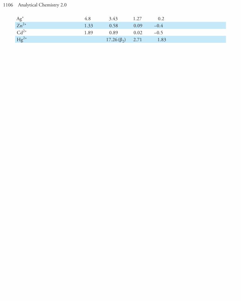
Appendix 12: Formation ConstantsThe following table provides Ki and bi values for selected metal–ligand complexes, arranged by the ligand. All values are from Martell, A. E.; Smith, R. M. Critical Stability Constants, Vols. 1–4. Plenum Press: New York, 1976. Unless otherwise stated, values are for 25 oC and zero ionic strength. Those values in brackets are considered less reliable.

AcetateCH3COO– log K1 log K2 log K3 log K4 log K5 log K6

Mg2+ 1.27Ca2+ 1.18Ba2+ 1.07Mn2+ 1.40Fe2+ 1.40Co2+ 1.46Ni2+ 1.43Cu2+ 2.22 1.41Ag2+ 0.73 –0.09Zn2+ 1.57Cd2+ 1.93 1.22 –0.89Pb2+ 2.68 1.40

AmmoniaNH3 log K1 log K2 log K3 log K4 log K5 log K6

Ag+ 3.31 3.91

Co2+ (T = 20 oC) 1.99 1.51 0.93 0.64 0.06 –0.73

Ni2+ 2.72 2.17 1.66 1.12 0.67 –0.03Cu2+ 4.04 3.43 2.80 1.48Zn2+ 2.21 2.29 2.36 2.03Cd2+ 2.55 2.01 1.34 0.84

ChlorideCl– log K1 log K2 log K3 log K4 log K5 log K6

Cu2+ 0.40Fe3+ 1.48 0.65

Ag+ (m = 5.0 M) 3.70 1.92 0.78 –0.3

Zn2+ 0.43 0.18 –0.11 –0.3Cd2+ 1.98 1.62 –0.2 –0.7Pb2+ 1.59 0.21 –0.1 –0.3

1103Appendices

CyanideCN– log K1 log K2 log K3 log K4 log K5 log K6

Fe2+ 35.4 (b6)Fe3+ 43.6 (b6)Ag+ 20.48 b2 0.92Zn2+ 11.07 b2 4.98 3.57Cd2+ 6.01 5.11 4.53 2.27Hg2+ 17.00 15.75 3.56 2.66Ni2+ 30.22 (b4)

EthylenediamineH2N

NH2 log K1 log K2 log K3 log K4 log K5 log K6

Ni2+ 7.38 6.18 4.11Cu2+ 10.48 9.07

Ag+ (T = 20 oC, m = 0.1 M) 4.700 3.00

Zn2+ 5.66 4.98 3.25Cd2+ 5.41 4.50 2.78

EDTA

NN

COO

COO

OOC

OOClog K1 log K2 log K3 log K4 log K5 log K6

Mg2+ (T = 20 oC, m = 0.1 M) 8.79

Ca2+ (T = 20 oC, m = 0.1 M) 10.69

Ba2+ (T = 20 oC, m = 0.1 M) 7.86

Bi3+ (T = 20 oC, m = 0.1 M) 27.8

Co2++ (T = 20 oC, m = 0.1 M) 16.31

Ni2+ (T = 20 oC, m = 0.1 M) 18.62

Cu2+ (T = 20 oC, m = 0.1 M) 18.80

Cr3+ (T = 20 oC, m = 0.1 M) [23.4]

Fe3+ (T = 20 oC, m = 0.1 M) 25.1

Ag+ (T = 20 oC, m = 0.1 M) 7.32

Zn2+ (T = 20 oC, m = 0.1 M) 16.50

Cd2+ (T = 20 oC, m = 0.1 M) 16.46

Hg2+ (T = 20 oC, m = 0.1 M) 21.7

Pb2+ (T = 20 oC, m = 0.1 M) 18.04


Al3+ (T = 20 oC, m = 0.1 M) 16.3

FluorideF– log K1 log K2 log K3 log K4 log K5 log K6

Al3+ (m = 0.5 M) 6.11 5.01 3.88 3.0 1.4 0.4

HydroxideOH– log K1 log K2 log K3 log K4 log K5 log K6

Al3+ 9.01 [9.69] [8.3] 6.0Co2+ 4.3 4.1 1.3 0.5Fe2+ 4.5 [2.9] 2.6 –0.4Fe3+ 11.81 10.5 12.1Ni2+ 4.1 3.9 3.Pb2+ 6.3 4.6 3.0Zn2+ 5.0 [6.1] 2.5 [1.2]

IodideI– log K1 log K2 log K3 log K4 log K5 log K6

Ag+ (T = 18 oC) 6.58 [5.12] [1.4]

Cd2+ 2.28 1.64 1.08 1.0Pb2+ 1.92 1.28 0.7 0.6

Nitriloacetate

NCOO

COO

OOC log K1 log K2 log K3 log K4 log K5 log K6

Mg2+ (T = 20 oC, m = 0.1 M) 5.41

Ca2+ (T = 20 oC, m = 0.1 M) 6.41

Ba2+ (T = 20 oC, m = 0.1 M) 4.82

Mn2+ (T = 20 oC, m = 0.1 M) 7.44

Fe2+ (T = 20 oC, m = 0.1 M) 8.33

Co2+ (T = 20 oC, m = 0.1 M) 10.38

Ni2+ (T = 20 oC, m = 0.1 M) 11.53

Cu2+ (T = 20 oC, m = 0.1 M) 12.96

Fe3+ (T = 20 oC, m = 0.1 M) 15.9

Zn2+ (T = 20 oC, m = 0.1 M) 10.67

1105Appendices

Cd2+ (T = 20 oC, m = 0.1 M) 9.83

Pb2+ (T = 20 oC, m = 0.1 M) 11.39

OxalateC2O4

2– log K1 log K2 log K3 log K4 log K5 log K6

Ca2+ (m = 1 M) 1.66 1.03

Fe2+ (m = 1 M) 3.05 2.10

Co2+ 4.72 2.28Ni2+ 5.16Cu2+ 6.23 4.04

Fe3+ (m = 0.5 M) 7.53 6.11 4.85

Zn2+ 4.87 2.78

1,10-Phenanthroline

N N log K1 log K2 log K3 log K4 log K5 log K6

Fe2+ 20.7 (b3)

Mn2+ (m = 0.1 M) 4.0 3.3 3.0

Co2+ (m = 0.1 M) 7.08 6.64 6.08

Ni2+ 8.6 8.1 7.6Fe3+ 13.8 (b3)

Ag+ (m = 0.1 M) 5.02 7.04

Zn2+ 6.2 [5.9] [5.2]

ThiosulfateS2O3

2– log K1 log K2 log K3 log K4 log K5 log K6

Ag+ (T = 20 oC) 8.82 4.85 0.53

ThiocyanateSCN– log K1 log K2 log K3 log K4 log K5 log K6

Mn2+ 1.23Fe2+ 1.31Co2+ 1.72Ni2+ 1.76Cu2+ 2.33Fe3+ 3.02


Ag+ 4.8 3.43 1.27 0.2Zn2+ 1.33 0.58 0.09 –0.4Cd2+ 1.89 0.89 0.02 –0.5Hg2+ 17.26 (b2) 2.71 1.83

1107Appendices

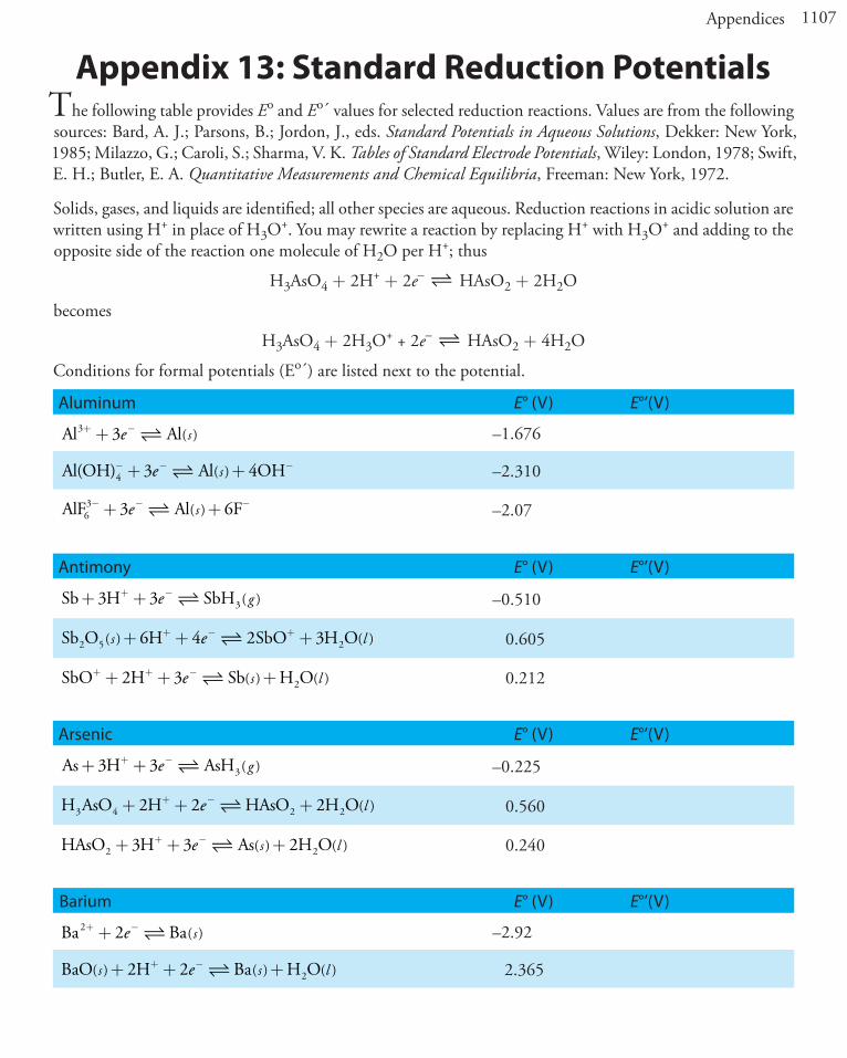
Appendix 13: Standard Reduction PotentialsThe following table provides Eo and Eo´ values for selected reduction reactions. Values are from the following sources: Bard, A. J.; Parsons, B.; Jordon, J., eds. Standard Potentials in Aqueous Solutions, Dekker: New York, 1985; Milazzo, G.; Caroli, S.; Sharma, V. K. Tables of Standard Electrode Potentials, Wiley: London, 1978; Swift, E. H.; Butler, E. A. Quantitative Measurements and Chemical Equilibria, Freeman: New York, 1972.

Solids, gases, and liquids are identified; all other species are aqueous. Reduction reactions in acidic solution are written using H+ in place of H3O+. You may rewrite a reaction by replacing H+ with H3O+ and adding to the opposite side of the reaction one molecule of H2O per H+; thus

H3AsO4 + 2H+ + 2e– HAsO2 + 2H2O

becomes

H3AsO4 + 2H3O+ + 2e– HAsO2 + 4H2O

Conditions for formal potentials (Eo´) are listed next to the potential.

Aluminum E° (V) E°’(V)

Al Al3 3+ −+ e s ( ) –1.676

Al(OH) Al OH4 3 4− − −+ +e s ( ) –2.310

AlF Al F63 3 6− − −+ +e s ( ) –2.07

Antimony E° (V) E°’(V)

Sb H SbH+ ++ −3 3 3e g ( ) –0.510

Sb O H SbO H O5 22 6 4 2 3( ) ( )s le+ + ++ − + 0.605

SbO H Sb H O2+ + −+ + +2 3e s l ( ) ( ) 0.212

Arsenic E° (V) E°’(V)

As H AsH+ ++ −3 3 3e g ( ) –0.225

H AsO H HAsO H O3 24 22 2 2+ + ++ −e l ( ) 0.560

HAsO H As H O22 3 3 2+ + ++ −e s l ( ) ( ) 0.240

Barium E° (V) E°’(V)

Ba Ba2 2+ −+ e s ( ) –2.92

BaO H Ba H O2( ) ( ) ( )s s le+ + ++ −2 2 2.365


Beryllium E° (V) E°’(V)

Be Be2 2+ −+ e s ( ) –1.99

Bismuth E° (V) E°’(V)

Bi Bi3 3+ −+ e s ( ) 0.317

BiCl Bi Cl4 3 4− − −+ +e s ( ) 0.199

Boron E° (V) E°’(V)

B(OH H B H O2) ( ) ( )3 3 3 3+ + ++ −e s l –0.890

B(OH B OH) ( )4 3 4− − −+ +e s –1.811

Bromine E° (V) E°’(V)

Br Br2 +− −2 2e 1.087

HOBr H Br H O2+ + ++ − −2e l ( ) 1.341

HOBr H Br H O2+ + ++ − −e l

12 ( ) 1.604

BrO H O Br OH2− − − −+ + +( )l e2 2 0.76 in 1 M NaOH

BrO H Br H O231

2 26 5 3− + −+ + +e l ( ) 1.5

BrO H Br H O23 6 6 3− + − −+ + +e 1.478

Cadmium E° (V) E°’(V)

Cd Cd2 2+ −+ e s ( ) –0.4030

Cd(CN) Cd CN42 2 4− − −+ +e s ( ) –0.943

Cd(NH ) Cd NH3 42

32 4+ −+ +e s ( ) –0.622

Calcium E° (V) E°’(V)

Ca Ca2 2+ −+ e s ( ) –2.84

1109Appendices

Carbon E° (V) E°’(V)

CO H CO H O22 2 2( ) ( ) ( )g g le+ + ++ − –0.106

CO H HCO H22 2 2( )g e+ ++ − –0.20

2 2 22 2 2 4CO H H C O( )g e+ ++ − –0.481

HCHO H CH OH+ ++ −2 2 3e 0.2323

Cerium E° (V) E°’(V)

Ce Ce3 3+ −+ e s ( ) –2.336

Ce Ce4 3+ − ++ e 1.72

1.70 in 1 M HClO41.44 in 1 M H2SO41.61 in 1 M HNO31.28 in 1 M HCl

Chlorine E° (V) E°’(V)

Cl Cl2 2 2( )g e+ − − 1.396

ClO H O Cl OH2− − −+ + +( ) ( )l ge

12 2 2 0.421 in 1 M NaOH

ClO H O Cl OH2− − − −+ + +( )l e2 2 0.890 in 1 M NaOH

HClO H HOCl H O22 2 2+ + ++ −e 1.64

ClO H ClO H O23 22− + −+ + +e g ( ) 1.175

ClO H HClO H O23 23 2− + −+ + +e 1.181

ClO H ClO H O24 32 2− + − −+ + +e 1.201

Chromium E° (V) E°’(V)

Cr Cr3 2+ − ++ e –0.424

Cr Cr2 2+ −+ e s ( ) –0.90

Cr O H Cr H O22 72 314 6 2 7− + − ++ + +e l ( ) 1.36

CrO H O Cr OH OH242

44 3 2 4− − − −+ + +( ) ( )l e –0.13 in 1 M NaOH


Cobalt E° (V) E°’(V)

Co Co2 2+ −+ e s ( ) –0.277

Co Co3 2+ − ++ e 1.92

Co(NH Co(NH3 63

3 62) )+ − ++ e 0.1

Co(OH Co(OH OH) )( ) ( )3 2s se+ +− − 0.17

Co(OH Co OH) ( ) ( )2 2 2s se+ +− − –0.746

Copper E° (V) E°’(V)

Cu Cu+ −+ e s ( ) 0.520

Cu Cu2+ − ++ e 0.159

Cu Cu2 2+ −+ e s ( ) 0.3419

Cu I CuI2+ − −+ + e s ( ) 0.86

Cu Cl CuCl2+ − −+ + e s ( ) 0.559

Fluorine E° (V) E°’(V)

F H HF2 2 2 2( )g e+ ++ − 3.053

F F2 2 2( )g e++ − − 2.87

Gallium E° (V) E°’(V)

Ga Ga3 3+ −+ e s ( )

Gold E° (V) E°’(V)

Au Au+ −+ e s ( ) 1.83

Au Au3 2+ − ++ e 1.36

Au Au3 3+ −+ e s ( ) 1.52

AuCl Au Cl4 3 4− − −+ +e s ( ) 1.002

1111Appendices

Hydrogen E° (V) E°’(V)

2 2 2H H+ −+ e g ( ) 0.00000

H O H OH2 + +− −e g

12 2( ) –0.828

Iodine E° (V) E°’(V)

I I2 2 2( )s e+ − − 0.5355

I I3 2 3− − −+ e 0.536

HIO H I H O2+ + ++ − −2e l ( ) 0.985

IO H I H O231

2 26 5 3− + −+ + +e s l ( ) ( ) 1.195

IO H O I OH23 3 6 6− − − −+ + +( )l e 0.257

Iron E° (V) E°’(V)

Fe Fe2 2+ −+ e s ( ) –0.44

Fe Fe3 3+ −+ e s ( ) –0.037

Fe Fe3 2+ − ++ e 0.771

0.70 in 1 M HCl0.767 in 1 M HClO40.746 in 1 M HNO30.68 in 1 M H2SO40.44 in 0.3 M H3PO4

Fe(CN) Fe(CN)63

64− − −+ e 0.356

Fe(phen) Fe(phen)63

62+ − ++ e 1.147

Lanthanum E° (V) E°’(V)

La La3 3+ −+ e s ( ) –2.38

Lead E° (V) E°’(V)

Pb Pb2 2+ −+ e s ( ) –0.126

PbO OH Pb H O2224 2 2( ) ( )s le+ + +− − +

1.46

PbO O H PbSO H O22 42

44 4 2 2( ) ( ) ( )s s lS e+ + + +− + − 1.690

PbSO Pb SO4 422( ) ( )s se+ +− −

–0.356


Lithium E° (V) E°’(V)

Li Li+ −+ e s ( ) –3.040

Magnesium E° (V) E°’(V)

Mg Mg2 2+ −+ e s ( ) –2.356

Mg(OH) Mg OH2 2 2( ) ( )s se+ +− − –2.687

Manganese E° (V) E°’(V)

Mn Mn2 2+ −+ e s ( ) –1.17

Mn Mn3 2+ − ++ e 1.5

MnO H Mn H O2224 2 2( ) ( )s le+ + ++ − +

1.23

MnO H MnO H O24 24 3 2− + −+ + +e s l ( ) ( ) 1.70

MnO H Mn H O2428 5 4− + − ++ + +e l ( ) 1.51

MnO H O MnO OH24 22 3 4− − −+ + +( ) ( )l se 0.60

Mercury E° (V) E°’(V)

Hg Hg2 2+ −+ e l ( ) 0.8535

2 2222Hg Hg+ − ++ e 0.911

Hg Hg22 2 2+ −+ e l ( ) 0.7960

Hg Cl Hg Cl2 2 2 2 2( ) ( )s le+ +− − 0.2682

HgO H Hg H O2( ) ( ) ( )s l le+ + ++ −2 2 0.926

Hg Br Hg Br2 2 2 2 2( ) ( )s le+ +− − 1.392

Hg I Hg I2 2 2 2 2( ) ( )s le+ +− − –0.0405

1113Appendices

Molybdenum E° (V) E°’(V)

Mo Mo3 3+ −+ e s ( ) –0.2

MoO H Mo H O22 4 4 2( ) ( ) ( )s s le+ + ++ − –0.152

MoO H O Mo OH242 4 6 8− − −+ + +( ) ( )l se –0.913

Nickel E° (V) E°’(V)

Ni Ni2 2+ −+ e s ( ) –0.257

Ni OH Ni OH( ) ( )2 2 2+ +− −e s –0.72

Ni NH Ni NH( ) ( )3 62

32 6+ −+ +e s –0.49

Nitrogen E° (V) E°’(V)

N H N H22 55 4( )g e+ ++ − + –0.23

N O H N H O22 22 2( ) ( ) ( )g g le+ + ++ − 1.77

2 2 2 2NO H N O H O2( ) ( ) ( )g g le+ + ++ − 1.59

HNO H NO H O22 + + ++ −e g l ( ) ( ) 0.996

2 4 4 32 2HNO H N O H O2+ + ++ −e g l ( ) ( ) 1.297

NO H NO H O2 23 3 2− + −+ + +e H l ( ) 0.94

Oxygen E° (V) E°’(V)

O H H O2 22 2 2( )g e+ ++ − 0.695

O H H O22 4 4 2( ) ( )g le+ ++ − 1.229

H O H H O22 2 2 2 2+ ++ −e l ( ) 1.763

O H O OH22 2 4 4( ) ( )g l e+ + − − 0.401

O H O H O23 22 2( ) ( ) ( )g g le+ + ++ − 2.07


Phosphorous E° (V) E°’(V)

P H PHwhite( , ) ( )s ge+ ++ −3 3 3

H PO H H PO H O3 3 3 2 2+ + ++ −2 2e l ( )

H PO H H PO H O3 3 24 32 2+ + ++ −e l ( )

Platinum E° (V) E°’(V)

Pt Pt2 2+ −+ e s ( )

PtCl Pt Cl42 2 4− − −+ +e s ( )

Potassium E° (V) E°’(V)

K K+ −+ e s ( )

Ruthenium E° (V) E°’(V)

Ru Ru3 2+ − ++ e 0.249

RuO H Ru H O22 4 4 2( ) ( ) ( )s s le+ + ++ − 0.68

Ru NH Ru Ru NH( ) ( )( )3 63

3 62+ − ++ +e s 0.10

Ru CN Ru Ru CN( ) ( )( )63

64− − −+ +e s 0.86

Selenium E° (V) E°’(V)

Se Se( )s e+ − −2 2 –0.67 in 1 M NaOH

Se H H Se( ) ( )s ge+ ++ −2 2 2 –0.115

H SeO H Se H O22 3 4 4 3+ + ++ −e s l ( ) ( ) 0.74

SeO H H SeO H O243

2 34− + −+ + +e l ( ) 1.151

Silicon E° (V) E°’(V)

SiF Si F62 4 6− − −+ +e s ( ) –1.37

SiO H Si H O22 4 4 2( ) ( ) ( )s s le+ + ++ − –0.909

SiO H SiH H O22 48 8 2( ) ( ) ( )s g le+ + ++ − –0.516

1115Appendices

Silver E° (V) E°’(V)

Ag Ag+ −+ e s ( ) 0.7996

AgBr Ag Br( ) ( )s se+ +− − 0.071

Ag C O Ag C O2 2 4 2 422 2( ) ( )s se+ +− −

0.47

AgCl Ag Cl( ) ( )s se+ +− − 0.2223

AgI Ag I( ) ( )s se+ +− − –0.152

Ag S Ag S222 2( ) ( )s se+ +− −

–0.71

Ag NH Ag NH( ) ( )3 2 32+ −+ +e s –0.373

Sodium E° (V) E°’(V)

Na Na+ −+ e s ( ) –2.713

Strontium E° (V) E°’(V)

Sr Sr2 2+ −+ e s ( ) –2.89

Sulfur E° (V) E°’(V)

S S( )s e+ − −2 2 –0.407

S H H S( )s e+ ++ −2 2 2 0.144

S O H H SO2 62

2 34 2 2− + −+ + e 0.569

S O SO2 82

422 2− − −+ e 1.96

S O S O4 62

2 322 2− − −+ e 0.080

2 2 2 432

2 42SO H O S O OH2

− − − −+ + +( )l e –1.13

2 3 4 632

2 32SO H O S O OH2

− − − −+ + +( )l e –0.576 in 1 M NaOH

2 4 2 242

2 62SO H S O H O2

− + − −+ + +e l ( ) –0.25

SO H O SO OH242

322 2− − − −+ + +( )l e –0.936

SO H H SO H O242

2 324 2− + − −+ ++ +e l ( ) 0.172


Thallium E° (V) E°’(V)

Tl Tl3 2+ − ++ e

1.25 in 1 M HClO40.77 in 1 M HCl

Tl Tl3 3+ −+ e s ( ) 0.742

Tin E° (V) E°’(V)

Sn Sn2 2+ −+ e s ( ) –0.19 in 1 M HCl

Sn Sn4 22+ − ++ e 0.154 0.139 in 1 M HCl

Titanium E° (V) E°’(V)

Ti Ti2 2+ −+ e s ( ) –0.163

Ti Ti3 2+ − ++ e –0.37

Tungsten E° (V) E°’(V)

WO H W H O22 4 4 2( ) ( ) ( )s s le+ + ++ − –0.119

WO H W H O23 6 6 3( ) ( ) ( )s s le+ + ++ − –0.090

Uranium E° (V) E°’(V)

U U3 3+ −+ e s ( ) –1.66

U U4 3+ − ++ e –0.52

UO H U H O2244 2+ + − ++ + +e l ( ) 0.27

UO UO22

2+ − ++ e 0.16

UO H U H O222 44 2 2+ + − ++ + +e l ( ) 0.327

Vanadium E° (V) E°’(V)

V V2 2+ −+ e s ( ) –1.13

V V3 2+ − ++ e –0.255

VO H V H O22 32+ + − ++ + +e l ( ) 0.337

VO H VO H O222 22+ + − ++ + +e l ( ) 1.000

1117Appendices

Zinc E° (V) E°’(V)

Zn Zn2 2+ −+ e s ( ) –0.7618

Zn(OH) Zn OH42 2 4− − −+ +e s ( ) –1.285

Zn(NH ) Zn NH3 42

32 4+ −+ +e s ( ) –1.04

Zn(CN) Zn CN42 2 4− −+ +e s ( ) –1.34


Appendix 14: Random Number TableThe following table provides a list of random numbers in which the digits 0 through 9 appear with approxi-mately equal frequency. Numbers are arranged in groups of five to make the table easier to view. This arrange-ment is arbitrary, and you can treat the table as a sequence of random individual digits (1, 2, 1, 3, 7, 4…going down the first column of digits on the left side of the table), as a sequence of three digit numbers (111, 212, 104, 367, 739… using the first three columns of digits on the left side of the table), or in any other similar manner. Let’s use the table to pick 10 random numbers between 1 and 50. To do so, we choose a random starting point, perhaps by dropping a pencil onto the table. For this exercise, we will assume that the starting point is the fifth row of the third column, or 12032. Because the numbers must be between 1 and 50, we will use the last two digits, ignoring all two-digit numbers less than 01 or greater than 50, and rejecting any duplicates. Proceeding down the third column, and moving to the top of the fourth column when necessary, gives the following 10 random numbers: 32, 01, 05, 16, 15, 38, 24, 10, 26, 14.These random numbers (1000 total digits) are a small subset of values from the publication Million Random Digits (Rand Corporation, 2001) and used with permission. Information about the publication, and a link to a text file containing the million random digits is available at http://www.rand.org/pubs/monograph_reports/MR1418/.

11164 36318 75061 37674 26320 75100 10431 20418 19228 9179221215 91791 76831 58678 87054 31687 93205 43685 19732 0846810438 44482 66558 37649 08882 90870 12462 41810 01806 0297736792 26236 33266 66583 60881 97395 20461 36742 02852 5056473944 04773 12032 51414 82384 38370 00249 80709 72605 6749749563 12872 14063 93104 78483 72717 68714 18048 25005 0415164208 48237 41701 73117 33242 42314 83049 21933 92813 0476351486 72875 38605 29341 80749 80151 33835 52602 79147 0886899756 26360 64516 17971 48478 09610 04638 17141 09227 1060671325 55217 13015 72907 00431 45117 33827 92873 02953 8547465285 97198 12138 53010 95601 15838 16805 61004 43516 1702017264 57327 38224 29301 31381 38109 34976 65692 98566 2955095639 99754 31199 92558 68368 04985 51092 37780 40261 1447961555 76404 86210 11808 12841 45147 97438 60022 12645 6200078137 98768 04689 87130 79225 08153 84967 64539 79493 7491762490 99215 84987 28759 19177 14733 24550 28067 68894 3849024216 63444 21283 07044 92729 37284 13211 37485 10415 3645716975 95428 33226 55903 31605 43817 22250 03918 46999 9850159138 39542 71168 57609 91510 77904 74244 50940 31553 6256229478 59652 50414 31966 87912 87514 12944 49862 96566 48825

http://www.rand.org/pubs/monograph_reports/MR1418/

http://www.rand.org/pubs/monograph_reports/MR1418/

1119Appendices

Appendix 15: Polarographic Half-Wave Potentials

The following table provides E1/2 values for selected reduction reactions. Values are from Dean, J. A. Analyti-cal Chemistry Handbook, McGraw-Hill: New York, 1995.

Element E1/2 (volts vs. SCE) Matrix

Al Al3 3+ −+ e s ( ) –0.5 0.2 M acetate (pH 4.5–4.7)

Cd Cd2 2+ −+ e s ( ) –0.600.1 M KCl0.05 M H2SO41 M HNO3

Cr Cr3 3+ −+ e s ( )–0.35 (+3 → +2)–1.70 (+2 → 0)

1 M NH4Cl plus 1 M NH31 M NH4

+/NH3 buffer (ph 8–9)

Co Co3 3+ −+ e s ( )–0.5 (+3 → +2)–1.3 (+2 → 0) 1 M NH4Cl plus 1 M NH3

Co Co2 2+ −+ e s ( ) –1.03 1 M KSCN

Cu Cu2 2+ −+ e s ( )

0.04

–0.22

0.1 M KSCN0.1 M NH4ClO41 M Na2SO40.5 M potassium citrate (pH 7.5)

Fe Fe3 3+ −+ e s ( )–0.17 (+3 → +2)–1.52 (+2 → 0) 0.5 M sodium tartrate (pH 5.8)

Fe Fe3 2+ − ++ e –0.27 0.2 M Na2C2O4 (pH < 7.9)

Pb Pb2 2+ −+ e s ( )–0.405–0.435

1 M HNO31 M KCl

Mn Mn2 2+ −+ e s ( ) –1.65 1 M NH4Cl plus 1 M NH3

Ni Ni2 2+ −+ e s ( )–0.70–1.09

1 M KSCN1 M NH4Cl plus 1 M NH3

Zn Zn2 2+ −+ e s ( )–0.995–1.33

0.1 M KCl1 M NH4Cl plus 1 M NH3


Appendix 16: Countercurrent SeparationsIn 1949, Lyman Craig introduced an improved method for separating analytes with similar distribution ratios.1 The technique, which is known as a countercurrent liquid–liquid extraction, is outlined in Figure A16.1 and discussed in detail below. In contrast to a sequential liquid–liquid extraction, in which we repeatedly extract the sample containing the analyte, a countercurrent extraction uses a serial extraction of both the sample and the extracting phases. Although countercurrent separations are no longer common—chromatographic separa-tions are far more efficient in terms of resolution, time, and ease of use—the theory behind a countercurrent extraction remains useful as an introduction to the theory of chromatographic separations.

To track the progress of a countercurrent liquid-liquid extraction we need to adopt a labeling convention. As shown in Figure A16.1, in each step of a countercurrent extraction we first complete the extraction and then transfer the upper phase to a new tube containing a portion of the fresh lower phase. Steps are labeled sequentially beginning with zero. Extractions take place in a series of tubes that also are labeled sequentially, starting with zero. The upper and lower phases in each tube are identified by a letter and number, with the letters U and L representing, respectively, the upper phase and the lower phase, and the number indicating the step in the countercurrent extraction in which the phase was first introduced. For example, U0 is the upper phase introduced at step 0 (during the first extraction), and L2 is the lower phase introduced at step 2 (during the third extraction). Finally, the partitioning of analyte in any extraction tube results in a fraction p remaining in the upper phase, and a fraction q remaining in the lower phase. Values of q are calculated using equation A16.1, which is identical to equation 7.26 in Chapter 7.

( )((

qV

DV Vaqaq

org aq

moles aq)moles aq)1

1

0

= =+ A16.1

The fraction p, of course is equal to 1 – q. Typically Vaq and Vorg are equal in a countercurrent extraction, al-though this is not a requirement.

Let’s assume that the analyte we wish to isolate is present in an aqueous phase of 1 M HCl, and that the organic phase is benzene. Because benzene has the smaller density, it is the upper phase, and 1 M HCl is the lower phase. To begin the countercurrent extraction we place the aqueous sample containing the analyte in tube 0 along with an equal volume of benzene. As shown in Figure A16.1a, before the extraction all the analyte is present in phase L0. When the extraction is complete, as shown in Figure A16.1b, a fraction p of the analyte is present in phase U0, and a fraction q is in phase L0. This completes step 0 of the countercurrent extraction. If we stop here, there is no difference between a simple liquid–liquid extraction and a countercurrent extraction.

After completing step 0, we remove phase U0 and add a fresh portion of benzene, U1, to tube 0 (see Figure A16.1c). This, too, is identical to a simple liquid-liquid extraction. Here is where the power of the countercur-rent extraction begins—instead of setting aside the phase U0, we place it in tube 1 along with a portion of analyte-free aqueous 1 M HCl as phase L1 (see Figure A16.1c). Tube 0 now contains a fraction q of the analyte, and tube 1 contains a fraction p of the analyte. Completing the extraction in tube 0 results in a fraction p of its contents remaining in the upper phase, and a fraction q remaining in the lower phase. Thus, phases U1 and L0 now contain, respectively, fractions pq and q2 of the original amount of analyte. Following the same logic, it is easy to show that the phases U0 and L1 in tube 1 contain, respectively, fractions p2 and pq of analyte. This completes step 1 of the extraction (see Figure A16.1d). As shown in the remainder of Figure A16.1, the countercurrent extraction continues with this cycle of phase transfers and extractions.

1 Craig, L. C. J. Biol. Chem. 1944, 155, 519–534.

1121Appendices

Figure A16.1 Scheme for a countercurrent extraction: (a) The sample containing the analyte begins in L0 and is extracted with a fresh portion of the upper, or mobile phase; (b) The extraction takes place, transferring a fraction p of analyte to the upper phase and leaving a fraction q of analyte in the lower, or stationary phase; (c) When the extraction is complete, the upper phase is transferred to the next tube, which contains a fresh portion of the sample’s solvent, and a fresh portion of the upper phase is added to tube 0. In (d) through (g), the process continues, with the addition of two more tubes.

0

1

U0

L0

extract

pU0

L0q

0U1

L0q

transfer

newphase

newphase

newphase

newphase

newphase

newphase

extract extract

pqU1

L0q2

0U2

L0q2

extract extract

pq2U2

L0q3

0U3

L0q3

pU0

L10

p2

U0

L1pq

p2

U0

L20

p3

U0

L30

2p2qU1

L2p2q

pqU1

L1pq

2p2qU1

L12pq2

extract

p3

U0

L2p2q

pq2

U2

L12pq2

transfer

transfer

transfer

transfer

transfer

(a)

(b)

(c)

(d)

(e)

(f )

(g)

Tube 0 Tube 1 Tube 2 Tube 3


In a countercurrent liquid–liquid extraction, the lower phase in each tube remains in place, and the upper phase moves from tube 0 to successively higher numbered tubes. We recognize this difference in the movement of the two phases by referring to the lower phase as a stationary phase and the upper phase as a mobile phase. With each transfer some of the analyte in tube r moves to tube r + 1, while a portion of the analyte in tube r – 1 moves to tube r. Analyte introduced at tube 0 moves with the mobile phase, but at a rate that is slower than the mobile phase because, at each step, a portion of the analyte transfers into the stationary phase. An analyte that preferentially extracts into the stationary phase spends proportionally less time in the mobile phase and moves at a slower rate. As the number of steps increases, analytes with different values of q eventually separate into completely different sets of extraction tubes.

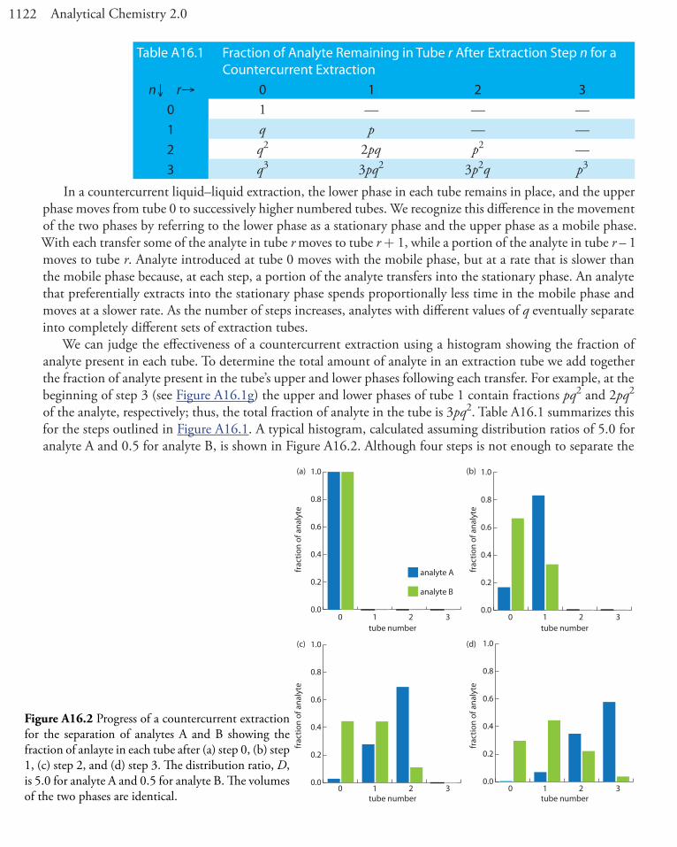
We can judge the effectiveness of a countercurrent extraction using a histogram showing the fraction of analyte present in each tube. To determine the total amount of analyte in an extraction tube we add together the fraction of analyte present in the tube’s upper and lower phases following each transfer. For example, at the beginning of step 3 (see Figure A16.1g) the upper and lower phases of tube 1 contain fractions pq2 and 2pq2 of the analyte, respectively; thus, the total fraction of analyte in the tube is 3pq2. Table A16.1 summarizes this for the steps outlined in Figure A16.1. A typical histogram, calculated assuming distribution ratios of 5.0 for analyte A and 0.5 for analyte B, is shown in Figure A16.2. Although four steps is not enough to separate the

Table A16.1 Fraction of Analyte Remaining in Tube r After Extraction Step n for a Countercurrent Extraction

n↓ r→ 0 1 2 30 1 — — —1 q p — —2 q2 2pq p2 —3 q3 3pq2 3p2q p3

Figure A16.2 Progress of a countercurrent extraction for the separation of analytes A and B showing the fraction of anlayte in each tube after (a) step 0, (b) step 1, (c) step 2, and (d) step 3. The distribution ratio, D, is 5.0 for analyte A and 0.5 for analyte B. The volumes of the two phases are identical.

0.0

0.2

0.4

0.6

0.8

1.0

0.0

0.2

0.4

0.6

0.8

1.0

0.0

0.2

0.4

0.6

0.8

1.0

0.0

0.2

0.4

0.6

0.8

1.0

tube number tube number

tube numbertube number

0 1 2 3 0 1 2 3

0 1 2 3 0 1 2 3

frac

tion

of a

naly

tefr

actio

n of

ana

lyte

frac

tion

of a

naly

tefr

actio

n of

ana

lyte

analyte A

analyte B

(a) (b)

(c) (d)

1123Appendices

analytes in this instance, it is clear that if we extend the countercurrent extraction to additional tubes, we will eventually separate the analytes.

Figure A16.1 and Table A16.1 show how an analyte’s distribution changes during the first four steps of a countercurrent extraction. Now we consider how we can generalize these results to calculate the amount of analyte in any tube, at any step during the extraction. You may recognize the pattern of entries in Table A16.1 as following the binomial distribution

f r nn

n r rp qr n r( , )

!( )! !

=−

− A16.2

where f(r, n) is the fraction of analyte present in tube r at step n of the countercurrent extraction, with the upper phase containing a fraction p� f(r, n) of analyte and the lower phase containing a fraction q�f(r, n) of the analyte.

Example A16.1

The countercurrent extraction shown in Figure A16.2 is carried out through step 30. Calculate the fraction of analytes A and B in tubes 5, 10, 15, 20, 25, and 30.

SolutionTo calculate the fraction, q, for each analyte in the lower phase we use equation A6.1. Because the volumes of the lower and upper phases are equal, we get

qDA

A

=+

=+

=1

11

5 10 167.

q

DBB

=+

=+

=1

11

4 10 200.

Because we know that p + q = 1, we also know that pA is 0.833 and that pB is 0.333. For analyte A, the frac-tion in tubes 5, 10, 15, 20, 25, and 30 after the 30th step are

f ( , )!

( )! !( . ) ( . ) .5 30

3030 5 5

0 833 0 167 2 1 105 30 5=−

= ×− −115 0≈

f ( , )!

( )! !( . ) ( . ) .10 30

3030 10 10

0 833 0 167 110 30 10=−

=− 44 10 09× ≈−

f ( , )!

( )! !( . ) ( . ) .15 30

3030 15 15

0 833 0 167 215 30 15=−

=− 22 10 05× ≈−

f ( , )!

( )! !( . ) ( . ) .20 30

3030 20 20

0 833 0 167 020 30 20=−

=− 0013

f ( , )!

( )! !( . ) ( . ) .25 30

3030 25 25

0 833 0 167 025 30 25=−

=− 1192

f ( , )!

( )! !( . ) ( . ) .30 30

3030 30 30

0 833 0 167 030 30 30=−

=− 0004


The fraction of analyte B in tubes 5, 10, 15, 20, 25, and 30 is calculated in the same way, yielding respective values of 0.023, 0.153, 0.025, 0, 0, and 0. Figure A16.3, which provides the complete histogram for the dis-tribution of analytes A and B, shows that 30 steps is sufficient to separate the two analytes.

Constructing a histogram using equation A16.2 is tedious, particularly when the number of steps is large. Because the fraction of analyte in most tubes is approximately zero, we can simplify the histogram’s construc-tion by solving equation A16.2 only for those tubes containing an amount of analyte exceeding a threshold value. For a binomial distribution, we can use the mean and standard deviation to determine which tubes contain a significant fraction of analyte. The properties of a binomial distribution were covered in Chapter 4, with the mean, µ, and the standard deviation, s, given as

µ = np

σ= − =np p npq( )1

Furthermore, if both np and nq are greater than 5, the binomial distribution is closely approximated by the normal distribution and we can use the properties of a normal distribution to determine the location of the analyte and its recovery.2

Example A16.2

Two analytes, A and B, with distribution ratios of 9 and 4, respectively, are separated using a countercurrent extraction in which the volumes of the upper and lower phases are equal. After 100 steps determine the 99% confidence interval for the location of each analyte.

2 Mark, H.; Workman, J. Spectroscopy 1990, 5(3), 55–56.

Figure A16.3 Progress of a countercurrent ex-traction for the separation of analyte A and B showing the fraction of analyte in each tube af-ter 30 steips. The distribution ratio, D, is 5.0 for analyte A and 0.5 for analyte B. The volumes of the two phases are identical. See Example A16.1 for further details.

0.00

0.02

0.04

0.06

0.08

0.10

0.12

0.14

0.16

0.18

0.20 analyte A

analyte B

frac

tion

of a

naly

te

tube number0 5 10 15 20 25 30

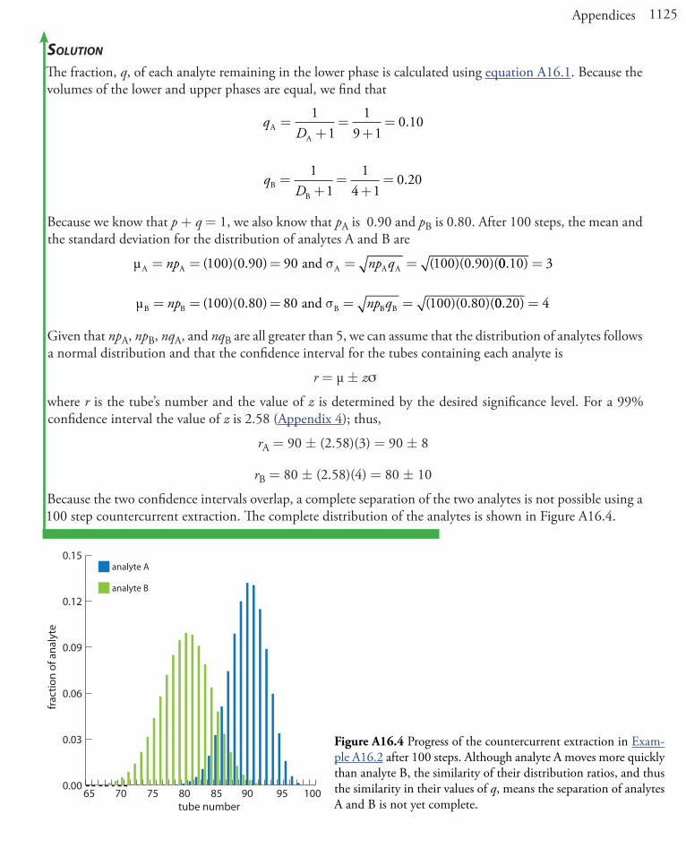
1125Appendices

SolutionThe fraction, q, of each analyte remaining in the lower phase is calculated using equation A16.1. Because the volumes of the lower and upper phases are equal, we find that

qDA

A

=+

=+

=1

11

9 10 10.

qDB

B

=+

=+

=1

11

4 10 20.

Because we know that p + q = 1, we also know that pA is 0.90 and pB is 0.80. After 100 steps, the mean and the standard deviation for the distribution of analytes A and B are

µ andA A A A A= = = = =np np q( )( . ) ( )( . )(100 0 90 90 100 0 90σ 00 10 3. ) =

µ andB B B B B= = = = =np np q( )( . ) ( )( . )(100 0 80 80 100 0 80σ 00 20 4. ) =

Given that npA, npB, nqA, and nqB are all greater than 5, we can assume that the distribution of analytes follows a normal distribution and that the confidence interval for the tubes containing each analyte is

r = µ ± zs

where r is the tube’s number and the value of z is determined by the desired significance level. For a 99% confidence interval the value of z is 2.58 (Appendix 4); thus,

rA = 90 ± (2.58)(3) = 90 ± 8

rB = 80 ± (2.58)(4) = 80 ± 10

Because the two confidence intervals overlap, a complete separation of the two analytes is not possible using a 100 step countercurrent extraction. The complete distribution of the analytes is shown in Figure A16.4.

Figure A16.4 Progress of the countercurrent extraction in Exam-ple A16.2 after 100 steps. Although analyte A moves more quickly than analyte B, the similarity of their distribution ratios, and thus the similarity in their values of q, means the separation of analytes A and B is not yet complete.

0.00

0.03

0.06

0.09

0.12

0.15analyte A

analyte B

frac

tion

of a

naly

te

tube number65 70 75 80 85 90 10095


Example A16.3

For the countercurrent extraction in Example A16.2, calculate the recovery and separation factor for analyte A if the contents of tubes 85–99 are pooled together.

SolutionFrom Example A16.2 we know that after 100 steps of the countercurrent extraction, analyte A is normally distributed about tube 90 with a standard deviation of 3. To determine the fraction of analyte A in tubes 85–99, we use the single-sided normal distribution in Appendix 3 to determine the fraction of analyte in tubes 0–84, and in tube 100. The fraction of analyte A in tube 100 is determined by calculating the deviation z

zr

=−

=−

=µσ

99 903

3

and using the table in Appendix 3 to determine the corresponding fraction. For z = 3 this corresponds to 0.135% of analyte A. To determine the fraction of analyte A in tubes 0–84 we again calculate the deviation

zr

=−

=−

=−µσ

85 903

1 67.

From Appendix 3 we find that 4.75% of analyte A is present in tubes 0–84. Analyte A’s recovery, therefore, is

100% – 4.75% – 0.135% ≈ 95%

To calculate the separation factor we determine the recovery of analyte B in tubes 85–99 using the same gen-eral approach as for analyte A, finding that approximately 89.4% of analyte B remains in tubes 0–84 and that essentially no analyte B is in tube 100. The recover for B, therefore, is

100% – 89.4% – 0% ≈ 10.6%

and the separation factor is

SRR

B,AA

B

= = =10 695

0 112.

.

1127Appendices

Appendix 17: Review of Chemical KineticsA reaction’s equilibrium position defines the extent to which the reaction can occur. For example, we expect a reaction with a large equilibrium constant, such as the dissociation of HCl in water

HCl H O H O2 3 Cl( ) ( ) ( ) ( )aq l aq aq+ ++ −

to proceed nearly to completion. A large equilibrium constant, however, does not guarantee that a reaction will reach its equilibrium position. Many reactions with large equilibrium constants, such as the reduction of MnO4

– by H2O

4 2 4 44 2 2MnO H O MnO 3O OH2– ( ) ( ) ( ) ( ) ( )aq l s g aq+ + + −

do not occur to an appreciable extent. The study of the rate at which a chemical reaction approaches its equi-librium position is called kinetics.

A17.1 Chemical Reaction Rates

A study of a reaction’s kinetics begins with the measurement of its reaction rate. Consider, for example, the general reaction shown below, involving the aqueous solutes A, B, C, and D, with stoichiometries of a, b, c, and d.

a b c dA B C D+ + A17.1The rate, or velocity, at which this reaction approaches its equilibrium position is determined by following the change in concentration of one reactant or one product as a function of time. For example, if we monitor the concentration of reactant A, we express the rate as

Rddt

=−[A]

A17.2

where R is the measured rate expressed as a change in concentration of A as a function of time. Because a reac-tant’s concentration decreases with time, we include a negative sign so that the rate has a positive value.

We also can determine the rate by following the change in concentration of a product as a function of time, which we express as

′ =−Rddt[C]

A17.3

Rates determined by monitoring different species do not necessarily have the same value. The rate R in equation A17.2 and the rate R´ in equation A17.3 have the same value only if the stoichiometric coefficients of A and C in reaction A17.1 are identical. In general, the relationship between the rates R and R´ is

Rac

R= × ′

A17.2 The Rate Law

A rate law describes how a reaction’s rate is affected by the concentration of each species in the reaction mixture. The rate law for reaction A17.1 takes the general form of


R k= [ ] [ ] [ ] [ ] [ ]A B C D Eα β γ δ ε A17.4

where k is the rate constant, and a, b, g, d, and e are the reaction orders of the reaction for each species pres-ent in the reaction.

There are several important points about the rate law in equation A17.4. First, a reaction’s rate may depend on the concentrations of both reactants and products, as well as the concentration of a species that does not appear in the reaction’s overall stoichiometry. Species E in equation A17.4, for example, may be a catalyst that does not appear in the reaction’s overall stoichiometry, but which increases the reaction’s rate. Second, the reac-tion order for a given species is not necessarily the same as its stoichiometry in the chemical reaction. Reaction orders may be positive, negative, or zero, and may take integer or non-integer values. Finally, the reaction’s overall reaction order is the sum of the individual reaction orders for each species. Thus, the overall reaction order for equation A17.4 is a + b + g + d + e.

A17.3 Kinetic Analysis of Selected Reactions

In this section we review the application of kinetics to several simple chemical reactions, focusing on how we can use the integrated form of the rate law to determine reaction orders. In addition, we consider how we can determine the rate law for a more complex system.

First-order reactions

The simplest case we can treat is a first-order reaction in which the reaction’s rate depends on the concentra-tion of only one species. The best example of a first-order reaction is an irreversible thermal decomposition of a single reactant, which we represent as

A Products→ A17.5with a rate law of

Rddt

k=− =[

[A]

A] A17.6

The simplest way to demonstrate that a reaction is first-order in A, is to double the concentration of A and note the effect on the reaction’s rate. If the observed rate doubles, then the reaction must be first-order in A. Alternatively, we can derive a relationship between the concentration of A and time by rearranging equation A17.6 and integrating.

dk dt

[[

A]A]=−

dk dt

t t[[

[

[A]

A]A]

A]

0 0∫ ∫=− A17.7

Evaluating the integrals in equation A17.7 and rearranging

ln[[A]A]

t kt0

=− A17.8

ln[ ln[A] A]t kt=− + 0 A17.9

1129Appendices

shows that for a first-order reaction, a plot of ln[A]t versus time is linear with a slope of –k and a y-intercept of ln[A]0. Equation A17.8 and equation A17.9 are known as integrated forms of the rate law.

Reaction A17.5 is not the only possible form of a first-order reaction. For example, the reactionA B Products+ → A17.10

will follow first-order kinetics if the reaction is first-order in A and if the concentration of B does not affect the reaction’s rate. This may happen if the reaction’s mechanism involves at least two steps. Imagine that in the first step, A slowly converts to an intermediate species, C, which rapidly reacts with the remaining reactant, B, in one or more steps, to form the products.

A B slowB C Products (fast)

→+ →

( )

Because a reaction’s rate depends only on those species in the slowest step—usually called the rate-determining step—and any preceding steps, species B will not appear in the rate law.

second-order reactions

The simplest reaction demonstrating second-order behavior is

2A Products→

for which the rate law is

Rddt

k=− =[

[A]

A]2

Proceeding as we did earlier for a first-order reaction, we can easily derive the integrated form of the rate law.

dk dt

[A]A][ 2 =−

dk dt

t t[A]A]

A]

A]

[[

[

200

∫ ∫=−

1 1

0[ [A] A]t

kt= +

For a second-order reaction, therefore, a plot of [A]t–1 versus t is linear with a slope of k and a y-intercept of

[A]0–1. Alternatively, we can show that a reaction is second-order in A by observing the effect on the rate when

we change the concentration of A. In this case, doubling the concentration of A produces a four-fold increase in the reaction’s rate.

Example A17.1

The following data were obtained during a kinetic study of the hydration of p-methoxyphenylacetylene by measuring the relative amounts of reactants and products by NMR.1

1 Kaufman, D,; Sterner, C.; Masek, B.; Svenningsen, R.; Samuelson, G. J. Chem. Educ. 1982, 59, 885–886.


time (min) % p-methyoxyphenylacetylene67 85.9

161 70.0241 57.6381 40.7479 32.4545 27.7604 24

Determine whether this reaction is first-order or second-order in p-methoxyphenylacetylene.

SolutionTo determine the reaction’s order we plot ln(%pmethoxyphenylacetylene) versus time for a first-order reaction, and (%p-methoxyphenylacetylene)–1 versus time for a second-order reaction (see Figure A17.1). Because a straight-line for the first-order plot fits the data nicely, we conclude that the reaction is first-order in p-meth-oxyphenylacetylene. Note that when we plot the data using the equation for a second-order reaction, the data show curvature that does not fit the straight-line model.

Pseudo-order reactions and the method oF initial rates

Unfortunately, most reactions of importance in analytical chemistry do not follow the simple first-order or second-order rate laws discussed above. We are more likely to encounter the second-order rate law given in equation A17.11 than that in equation A17.10.

R k= [A][B] A17.11

0 100 200 300 400 500 600 7003.0

3.2

3.4

3.6

3.8

4.0

4.2

4.4

4.6

4.8

5.0

ln(p

-met

hoxy

phen

ylac

etyl

ene)

time (min) time (min)0 100 200 300 400 500 600 700

0.00

0.01

0.02

0.03

0.04

0.05

(p-m

etho

xyph

enyl

acet

ylen

e)–1

(a) (b)

�rst-order plot

second-order plot

Figure A17.1 Integrated rate law plots for the data in Example A17.1 assuming (a) first-order kinetics and (b) second-order kinetics.

1131Appendices

Demonstrating that a reaction obeys the rate law in equation A17.11 is complicated by the lack of a simple integrated form of the rate law. Often we can simplify the kinetics by carrying out the analysis under condi-tions where the concentrations of all species but one are so large that their concentrations remain effectively constant during the reaction. For example, if the concentration of B is selected such that [B] >> [A], then equation A17.11 simplifies to

R k= ′[A]

where the rate constant k´ is equal to k[B]. Under these conditions, the reaction appears to follow first-order kinetics in A and, for this reason we identify the reaction as pseudo-first-order in A. We can verify the reac-tion order for A using either the integrated rate law or by observing the effect on the reaction’s rate of chang-ing the concentration of A. To find the reaction order for B, we repeat the process under conditions where [A] >> [B].

A variation on the use of pseudo-ordered reactions is the initial rate method. In this approach we run a series of experiments in which we change one at a time the concentration of those species expected to affect the reaction’s rate and measure the resulting initial rate. Comparing the reaction’s initial rate for two experiments in which only the concentration of one species is different allows us to determine the reaction order for that species. The application of this method is outlined in the following example.

Example A17.2

The following data was collected during a kinetic study of the iodation of acetone by measuring the concentra-tion of unreacted I2 in solution.2

experiment number [C3H6O] (M) [H3O+] (M) [I2] (M) Rate (M s–1)1 1.33 0.0404 6.65�10–3 1.78�10–6

2 1.33 0.0809 6.65�10–3 3.89�10–6

3 1.33 0.162 6.65�10–3 8.11�10–6

4 1.33 0.323 6.65�10–3 1.66�10–5

5 0.167 0.323 6.65�10–3 1.64�10–6

6 0.333 0.323 6.65�10–3 3.76�10–6

7 0.667 0.323 6.65�10–3 7.55�10–6

8 0.333 0.323 3.32�10–3 3.57�10–6

SolutionThe order of the rate law with respect to the three reactants is determined by comparing the rates of two experi-ments in which there is a change in concentration for only one of the reactants. For example, in experiment 2 the [H3O+] and the rate are approximately twice as large as in experiment 1, indicating that the reaction is first-order in [H3O+]. Working in the same manner, experiments 6 and 7 show that the reaction is also first order with respect to [C3H6O], and experiments 6 and 8 show that the rate of the reaction is independent of the [I2]. Thus, the rate law is

R k= +[ ]C H O][H O3 6 3

2 Birk, J. P.; Walters, D. L. J. Chem. Educ. 1992, 69, 585–587.


To determine the value of the rate constant, we substitute the rate, the [C3H6O], and the [H3O+] for each experiment into the rate law and solve for k. Using the data from experiment 1, for example, gives a rate con-stant of 3.31�10–5 M–1 sec–1. The average rate constant for the eight experiments is 3.49�10–5 M–1 sec–1.

appendix - asdlib.org 11: acid–base dissociation constants appendix 12: metal–ligand formation...

Documents