U.U.D.M. Project Report 2011:17

Examensarbete i matematik, 15 hpHandledare och examinator: Sven Erick AlmJuni 2011

Department of MathematicsUppsala University

Apartment values in Uppsala: Significant factors that differentiate the selling prices

Johannes Krouthen

ABSTRACT

This study intends to see how different factors affect the selling prices for apartments in Uppsala. Regression and prediction is used to examine these effects. It will show that a few variables, such as the size and the distance to center can explain the biggest part of the price. But it also concludes that it is possible to find new variables from brokerage prospects which make an effect as well. An example of this is to see what type of condition the kitchen and the bathroom are in. Furthermore, this study shows how difficult it is to know which factors make an effect because of all the various correlations.

THANKS TO

Without Valueguard and most of all Lars-Erik Ericson this thesis would have been impossible to write. From Valueguard I would also like to thank David Magnusson for all the help with Stata and Håkan Toll for all his ideas. Thanks to Tomas Widerlöv for the prospects and of course a big thanks to my supervisor, Professor Sven-Erick Alm.

CONTENTS

Introduction ............................................................................................................................................. 1

Purpose ................................................................................................................................................ 1

Delimitation ......................................................................................................................................... 1

Valueguard .......................................................................................................................................... 1

Uppsala ................................................................................................................................................ 2

Method .................................................................................................................................................... 2

Regression ........................................................................................................................................... 2

Dummies.......................................................................................................................................... 2

Coefficient of determination ........................................................................................................... 3

Cross-validation ............................................................................................................................... 3

Selected data ....................................................................................................................................... 4

Variabels from Mäklarstatistik ........................................................................................................ 4

Variables from the prospects .......................................................................................................... 6

Critics on the data ........................................................................................................................... 7

Previous Studies ...................................................................................................................................... 7

Results ..................................................................................................................................................... 8

Regressions on the data from Mäklarstatistik .................................................................................... 8

The main variables........................................................................................................................... 8

Effect of the building year ............................................................................................................. 10

Effect of the district ....................................................................................................................... 10

The best possible regression from Mäklarstatistiks data .............................................................. 10

The effect of the variables found in the prospects ........................................................................... 11

Regressions .................................................................................................................................... 11

Difference in the predicted values ................................................................................................ 12

Conclusions ............................................................................................................................................ 15

Disscussion and ideas for future studies ............................................................................................... 17

References ............................................................................................................................................. 18

1

INTRODUCTION

The housing situation is always a topic and for some buyers that only want somewhere to live the market may seem like a jungle. Others use this complex situation as an opportunity to earn money by buying apartments only for the purpose of selling them at higher prices later on. No matter what the purpose of this investment is, there is indeed big money involved. To be sure that the apartment you buy is worth this money you have to ensure that it, not only satisfies your needs, but also that someone else is willing to pay for these needs later. But what are these needs? What makes people pay more for one apartment than another? How much is it worth to live those extra meters closer to the city and how much does it really add to the price if an apartment has a balcony or not?

PURPOSE

The thesis aims to distinguish which factors have a significant effect on an apartment’s value, in the purpose of predicting selling prices as accurately as possible.

DELIMITATION

The study will be made to predict prices of apartments in Uppsala and therefore the study will only be based on apartments sold in Uppsala. Apartments that have just been built will be excluded from analysis. The reason is that many of these objects are sold by the construction companies at fixed prices. The fees for these apartments are, in general, also higher than other similar apartments1. The study will also exclude the most expensive objects. These objects, which are often extreme penthouses or other special apartments, are too hard to predict in this model and may get a misleading prediction. For the same reason the study also excludes the absolute cheapest objects.

VALUEGUARD

Valueguard is a company that produces a new financial market around housing. They create price indexes for both apartments and houses for this purpose. The indexes for some regions in Sweden are already out on the Nasdaq OMX Stockholm stock exchange as the “NASDAQ OMX Valueguard-KTH (HOX) Sweden”. Their present goal is to get their market insurance out on the market as soon as possible, a product that will protect home owners against market risk. For risk management purpose they therefore need to be able to predict accurately how much specific houses and apartments are worth.2 This essay is a project in partnership together with Valueguard.

1 Lars-Erik Eriksson, Valueguard 2 Valueguard.se

2

UPPSALA

Uppsala is Sweden’s fourth biggest city and, as of December 31st 2010, its urban commune had a population of 197 787 people with the actual city having a population of 150 983 inhabitants.3 Since Uppsala is a student city with around 40 000 students4 a lot of these inhabitants are living in shared rooms, corridors, or rented apartment and the amount of people that live in co-operative flats is hard to predict. The city is located in the mainland so there is no coast, but through the whole city, a river called “Fyrisån” is flowing.

METHOD

REGRESSION

To make this model, regression analysis has been used. Regression analysis is used when you want to see how one dependent variable, also called the response variable, varies when you change the value in the independent or regressor variables5. The simplest kind of a regression model is the fitting of a straight line. In this type of regression which is called the first order model, the model only has one independent variable which the response variable is dependent of. However, in a lot of situations you can not describe your dependent variable with only one independent variable. You need many more. The general model for a multiple linear regression looks like:

,

where is the dependent variable, to are the regressors, to the parameters, n is the number of observations and is the random error with normal distribution N(0, σ2).6 For making the calculations, the statistical software package STATA has been used.

DUMMIES

In a lot of the factors it is not the specific value you want the model to use, it is whether it has the variable or not. For example if you want to examine the effect of a balcony the variable can only have the value zero or one and the parameter connected to that variable is only in use if it has an balcony. Such variables are called dummy variables or dummies7. But it is not only when the factor only can take two different outcomes that

3 http://www.uppsala.se/Upload/Dokumentarkiv/Externt/Dokument/Om_kommunen/Befolkningsutveckling/UppsalaexKN1920-2010.pdf 4 http://www.uu.se/node97 5 Montgomery p3 6 Montgomery p390 7 Draper&Smith p241

3

you produce dummies. Say that you want to examine the effect of different areas that flats are located in. In this case you can not only have one variable; you need one dummy for every area.

COEFFICIENT OF DETERMINATION

One of the best ways to see how well the regression approximates the data is to look at the Coefficient of determination, measures the “proportion of total variation about the mean, explained by the regression”. This means that you can see how well the regression approximates the data points. If you have an R2 of 100% it means that the regression line fits perfectly.8 But, because the always increases when we add terms to

the model, it is often better to use the adjusted , . The good thing with

is that it

only increases in value if a significant variable has been added to the model, and if

unnecessary terms are added the

will often decrease.

∑ (( )

)

∑ ( )

,

=1-(

) (

),

where p is the total number of independent variables and is the predicted value of the i:th observation .9

CROSS-VALIDATION

An important thing when doing a model in the purpose of predicting values is to test it on different data than the data you used when you made the model. This is because it is not certain that a significant “in-sample test” gives a significant “out-sample test”10. Sometimes this is a problem since you may have used all your data in the making of your model. The method used for solving this problem is Subsampling Cross-validation. This means that you randomly split your sample into two parts. The first part with K observations is for making your regression. The other part of the sample, the rest of the observations, is used as test observations. The random split should be repeated many times to reduce the variations and of course so that every observation has been predicted at least once. For every apartment that has been predicted more than one time the average prediction is calculated. The prediction error for every single apartment is then calculated as:

.

8 Draper&Smith p33 9 Montgomery p403 10 Inoue&Lutz p4

4

SELECTED DATA

VARIABELS FROM MÄKLARSTATISTIK

Most of the data that has been used comes from the company Mäklarstatistik11. Through them, Valueguard had access to around 14000 apartments that were sold between January 2005 and Mars 2011. In Figure 1 it is shown where the apartments were sold.

FIGURE 1: THE AREA OF WHERE THE OBSERVATIONS FROM MÄKLARSTATISTIK ARE COMING FROM. THE BLACK DOT INDICATES THE CENTER OF UPPSALA.

DEPENDENT VARIABLE

Price: Since the goal is to predict the price this is the dependent variable. The price is simply the price in SEK that the apartment was sold for. For making the model more accurate the prices are in logarithm form. This also makes the errors of the observations more normal distributed.

11 A company that provides information about sold houses and apartments in Sweden.

5

BASIC SPECIFICATION ABOUT THE APARTMENT

The Size of the apartment: The size of the apartment is measured in square meters.

The fee for the apartment: This variable is basically the fee per month for the apartment.

The number of rooms: In my data the apartments could have from one to seven rooms. If the apartment consisted of half rooms the data was rounded down to the closest integer.

The floor: This is the effect of which floor the apartment is situated at. The houses are divided in so many floors as the house consisted of. The specific effect of having an apartment on the top or bottom floor was also checked.

The number of floors in the building: It may be a significant difference of living in a high house than a low house. Therefore this variable is used to measure if the amount of floors in the house matters.

GEOGRAPHICAL VARIABLES

Distance to center: The distance to the center is measured in meters. Three different center positions are used; first a code was used that calculated the average position of the most expensive apartments. Then, the point that probably most people would consider as the city center was used. In the third test a circle around the big square is drawn and with different radii the distance to the circle is measured. Every apartment that was located inside the circle was given zero meters as distance. The reason is that it may not matter where in the center you live and that many people probably do not want to live in the absolute center.

City district: In this study, Uppsala is divided into approximately forty different districts to distinguish the different effects on each district.

The street: Some streets are more or less attractive than others. For example some of the streets are the main car roads in Uppsala and therefore have a lot of traffic. To get enough significance on this variable dummies are created only on the streets with at least forty observations on.

TIME ASPECTS

The year the apartment was built: Different time periods were used to see the effect of the apartment’s age. To get this variable as significant as possible the building years was divided into periods. Apartments which were built before 1920 got one dummy together and the rest of the years were divided in periods of five years each.

Selling date: Since the sample consists of apartments that were sold during several years, it was divided into 74 months. This variable is used more for the reason of making the other variables more significant than to explain the effect of it.

6

VARIABLES FROM THE PROSPECTS

The data from Mäklarstatistik did not consist of the entire information that was wanted. For example no information was given if the apartment had a balcony or not and nothing about the condition of the apartment. The brokerage Widerlöv has therefore provided more detailed information about the apartments. They delivered about 2000 prospects from apartments that have been put out for sale between May 2010 and Mars 2011 and also information about the sales price. The prospects included a lot of material that is not found in a regular database such as pictures on the apartment. Because of the time limit, 192 different objects from two different district of Uppsala, Luthagen and Fålhagen (see Figure 2) were selected. The reason for using apartments from two district and not randomly chosen apartments around the whole city was because the apartments close to each other have a lot in common and the new variables may easier show significance. The reason for choosing just Luthagen and Fålhagen was because there were most prospects from these areas. From the objects, three factors were selected that could have a significant effect on the price.

FIGURE 2: THE TWO AREAS INDICATE WHERE THE CHOSEN PROSPECTS CAME FROM. THE RED AREA INDICATES THE CHOSEN PART OF FÅLHAGEN AND THE BLACK AREA THE CHOSEN PART OF LUTHAGEN.

Balcony: Generally, apartments have no yards or gardens for themselves and a balcony could therefore be an exclusive addition to it. The study makes no distinction depending on the size or condition of the balcony. 127 of the observed apartments had balcony and 65 did not.

Fireplace: A fireplace is an interior that may make people pay a bit extra for the apartment. Like with the balcony variable all the fireplaces were valued equal. Twenty of the 192 tested apartments had fireplaces.

The kitchen and the bathroom: In the apartment prospects there are a lot of pictures from the different rooms and from these pictures you can estimate the condition of the apartment. The two rooms that were examined were the bathroom and the kitchen since

7

these rooms should be the most expensive rooms to fix. The prospects also consist of information about when these rooms where renovated and how new some of the appliances such as the dishwasher and fridge were. Both of these rooms were evaluated from one to three depending on their condition. A one is the best score and it meant that the room was newly renovated with relative new appliances. A score of two points for the room meant that the room was not in a direct need of fix but neither was it really newly renovated. If the room had a score of three it meant that most people probably would spend some money to renovate the room and that the apartment has old appliances. The total value of this variable is therefore between two and six. The observations were then divided into two groups. Apartments with a total grade of two or three were placed in the first group and apartments with a total grade between four and six in the other group. The apartments with the highest bathroom and kitchen standards are therefore in group one. Because of the time limit, this variable is only studied in the 109 observations from Fålhagen and not on the ones from Luthagen.

CRITICS ON THE DATA

The data from Mäklarstatistik is credible. However it only covers around 70% of the sold apartments during the time period and these 70% are from brokerages. Apartments that are sold privately, for example on Blocket are therefore excluded. These apartments may have different prices in general.

The same type of problem may occur with the apartments from Widerlöv’s prospects. Since all of these apartments are from the same brokerage, the variables may not correspond perfectly to the whole market.

PREVIOUS STUDIES

The housing situation and the apartment’s prices have interested many people, and a lot of people have tried to explain which the factors are that make us pay more for one apartment than another. Previous studies speculate that the size of the apartment has the absolute biggest impact on the price. This is, of course, not surprising. Some other more interesting results are the following.

Henrik Dennerheim has made a deep-diving analysis of housing prices in Södermalm in Stockholm and the factors that influence these prices. The data was based on 1336 sold apartments from between the years 2000 and 2006. In his models he gets the around 90 percent with highly significant coefficients. Some of his conclusions were the following.

The fee should have a coefficient of minus 0.26, which means that an increase in the fee of ten percent makes a decrease in price of 2.6 percent. Apartments on the first floor sells for on average 10% lower than apartments high up. He also writes that the effect of some factors is depending on how big the apartment is. If a three room apartment has been fully renovated he says that it increases the price by 12% but only by 7, 5% if it is a one room apartment. When it comes to the effect of the age of the house he concludes that apartments that were built around 1900 gives an average of 16% higher prices than apartments built after 1940.

8

One of the problems that Dennerheim discovered about his own study was that some apartments, like big penthouses are too attractive on the market so they should not be in this model; however these apartments were hard to pick out12.

Anna Flodström also made a prediction model on apartments in Stockholm and used data from 450 sales in the Stockholm city between the years 2006 and 2009. She mostly separated the models depending on how many rooms the apartment had. By using cross-validating she had a margin of error between 13%-17,5%, depending on the number of rooms13.

Mattias Karlsson and Mats Lövgren made a study on 600 apartments that were sold in central Uppsala from November 2008 to December 2009. They put their focus on trying to explain how much the fee and the location affects the price of the apartments. They concluded that the fee had a negative correlation to the price and that apartments tend to have a higher price not only if they were closer to the city but also if they were closer to the river that runs through Uppsala. They also saw a significant difference depending on which church parish the apartment belonged to, i.e. which part of town it is located in14.

RESULTS

REGRESSIONS ON THE DATA FROM MÄKLARSTATISTIK

THE MAIN VARIABLES

The main variables are: the size, distance to center, the selling date and the fee.

The apartment size is the variable which should have the biggest effect of the price. A

regression only including this variable had an of 41, 60 %. To exclude the effect of

when the apartment was sold the selling-date dummies was included in the test. These

variables made the increase to 58, 04%.

The next regression is made to weigh how accurate the model could be by only including the next two variables that was predicted as the most important; the distance to the city

center and the fee for the apartment. Of the three different ways of measuring the

distance to the center, the one with the circle around the center showed the best result. This variable showed better results when used in logarithmic form, probably because

12 Dennerheim 13 Flodström 14 Karlsson Lövgren

9

the importance of every meter to the center is decreasing as you get further away from the circle.

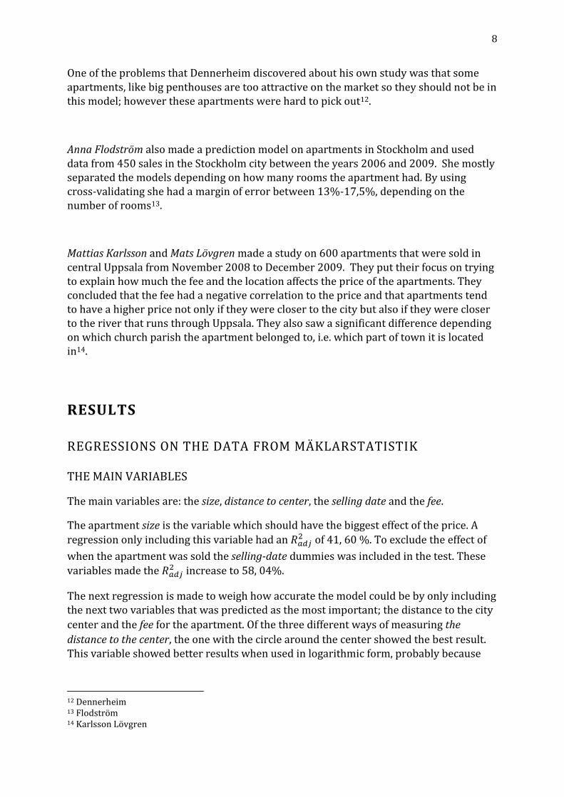
The test with the four factors had an of 77, 05% and a significance level better then

0,001 on the regression and all the variables.

Source | SS df MS Number of obs = 14437 -------------+------------------------------ F( 76, 14360) = 638.87 Model | 1690.35718 76 22.2415418 Prob > F = 0.0000 Residual | 499.929854 14360 0.034814057 R-squared = 0.7718 -------------+------------------------------ Adj R-squared = 0.7705 Total | 2190.28703 14436 0.151723956 Root MSE = 0.18659 ------------------------------------------------------------------------------ lnpris | Coef. Std. Err. t P>|t| [95% Conf. Interval] -------------+---------------------------------------------------------------- Size | 0.8206934 0.0069002 118.94 0.000 0.8071681 0.8342187 Fee | -0.0000529 2.39e-06 -22.09 0.000 -0.0000576 -0.0000482 Distance | -0.3075323 0.0028229 -108.94 0.000 -0.3130657 -0.301999 Constant | 12.71401 0.0322213 394.58 0.000 12.65085 12.77717

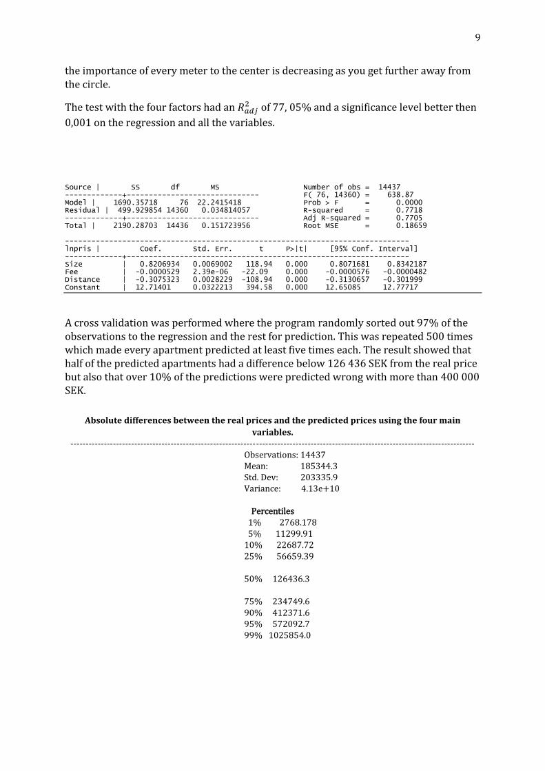
A cross validation was performed where the program randomly sorted out 97% of the observations to the regression and the rest for prediction. This was repeated 500 times which made every apartment predicted at least five times each. The result showed that half of the predicted apartments had a difference below 126 436 SEK from the real price but also that over 10% of the predictions were predicted wrong with more than 400 000 SEK.

Absolute differences between the real prices and the predicted prices using the four main

variables. -------------------------------------------------------------------------------------------------------------------------------------

Observations: 14437 Mean: 185344.3 Std. Dev: 203335.9

Variance: 4.13e+10

Percentiles 1% 2768.178 5% 11299.91 10% 22687.72 25% 56659.39

50% 126436.3

75% 234749.6 90% 412371.6 95% 572092.7 99% 1025854.0

10

EFFECT OF THE BUILDING YEAR

By only using the building year and the selling dates in the regression, had a value

of 27, 83%. However, together with the main variables, the raised to 81, 35% with

all except one dummy significant.

EFFECT OF THE DISTRICT

In this regression the building year factor was excluded and only the main variables and

the district variable were used. The raised to 83, 34% which is 6, 29% higher than

with only the main variables.

THE BEST POSSIBLE REGRESSION FROM MÄKLARSTATISTIKS DATA

This regression was based on all the discussed data from Mäklarstatistik. The of

the regression had an outcome of 88, 87 %. It could have been increased even higher but the variables would then have lost too much significance. Some of the results of the regression are the following: The predicted price (in logarithm form) for living on the ground floor is 0.0165 less than if you lived on the top floor. That means for example that for an apartment with a selling price of 1500000 SEK on the ground floor would then be predicted 1525000 SEK on the top floor if everything else was equal. Furthermore, from the same test we can conclude that the predicted price shifts a lot depending on how many rooms the apartment has even if the size of the apartments is equal. A one room apartment with a selling price of 1000000 SEK would for example be predicted to 1 040 000 SEK if it would have two rooms.

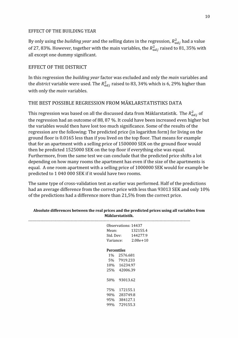
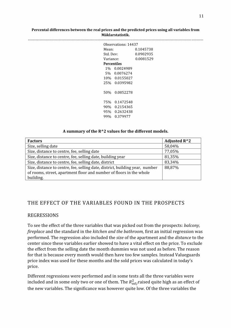
The same type of cross-validation test as earlier was performed. Half of the predictions had an average difference from the correct price with less than 93013 SEK and only 10% of the predictions had a difference more than 21,5% from the correct price.

Absolute differences between the real prices and the predicted prices using all variables from

Mäklarstatistik. --------------------------------------------------------------------------------------------------------------------------

Observations: 14437 Mean: 132155.4 Std. Dev: 144277.9

Variance: 2.08e+10

Percentiles 1% 2576.681 5% 7919.233 10% 16234.97 25% 42006.39

50% 93013.62

75% 172155.1 90% 283749.8 95% 384127.1 99% 729155.3

11

Percental differences between the real prices and the predicted prices using all variables from

Mäklarstatistik. ----------------------------------------------------------------------------------------------------------------------------------------

Observations: 14437 Mean: 0.1045738 Std. Dev: 0.0902935

Variance: 0.0081529 Percentiles 1% 0.0024989 5% 0.0076274 10% 0.0155027 25% 0.0395982

50% 0.0852278 75% 0.1472548 90% 0.2154365 95% 0.2632438 99% 0.379977

A summary of the R^2 values for the different models.

Factors Adjusted R^2 Size, selling date 58,04% Size, distance to centre, fee, selling date 77,05%

Size, distance to centre, fee, selling date, building year 81,35%

Size, distance to centre, fee, selling date, district 83,34% Size, distance to centre, fee, selling date, district, building year, number of rooms, street, apartment floor and number of floors in the whole building.

88,87%

THE EFFECT OF THE VARIABLES FOUND IN THE PROSPECTS

REGRESSIONS

To see the effect of the three variables that was picked out from the prospects: balcony,

fireplace and the standard in the kitchen and the bathroom, first an initial regression was

performed. The regression also included the size of the apartment and the distance to the center since these variables earlier showed to have a vital effect on the price. To exclude the effect from the selling date the month dummies was not used as before. The reason for that is because every month would then have too few samples. Instead Valueguards price index was used for these months and the sold prices was calculated in today’s price.

Different regressions were performed and in some tests all the three variables were

included and in some only two or one of them. The raised quite high as an effect of

the new variables. The significance was however quite low. Of the three variables the

12

fireplace seemed to have the clearest effect whereas the balcony and the kitchen and

bathroom variables showed almost no significant effect at all.

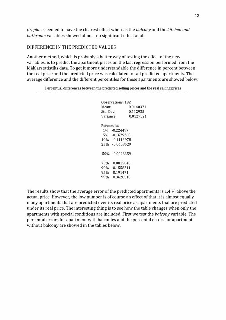
DIFFERENCE IN THE PREDICTED VALUES

Another method, which is probably a better way of testing the effect of the new variables, is to predict the apartment prices on the last regression performed from the Mäklarstatistiks data. To get it more understandable the difference in percent between the real price and the predicted price was calculated for all predicted apartments. The average difference and the different percentiles for these apartments are showed below:

Percentual differences between the predicted selling prices and the real selling prices -----------------------------------------------------------------------------------------------------------------------------

Observations: 192

Mean: 0.0140371 Std. Dev: 0.112925

Variance: 0.0127521

Percentiles 1% -0.224497 5% -0.1679368 10% -0.1113978 25% -0.0608529 50% -0.0028359 75% 0.0815048 90% 0.1558211 95% 0.191471 99% 0.3628518

The results show that the average error of the predicted apartments is 1.4 % above the actual price. However, the low number is of course an effect of that it is almost equally many apartments that are predicted over its real price as apartments that are predicted under its real price. The interesting thing is to see how the table changes when only the

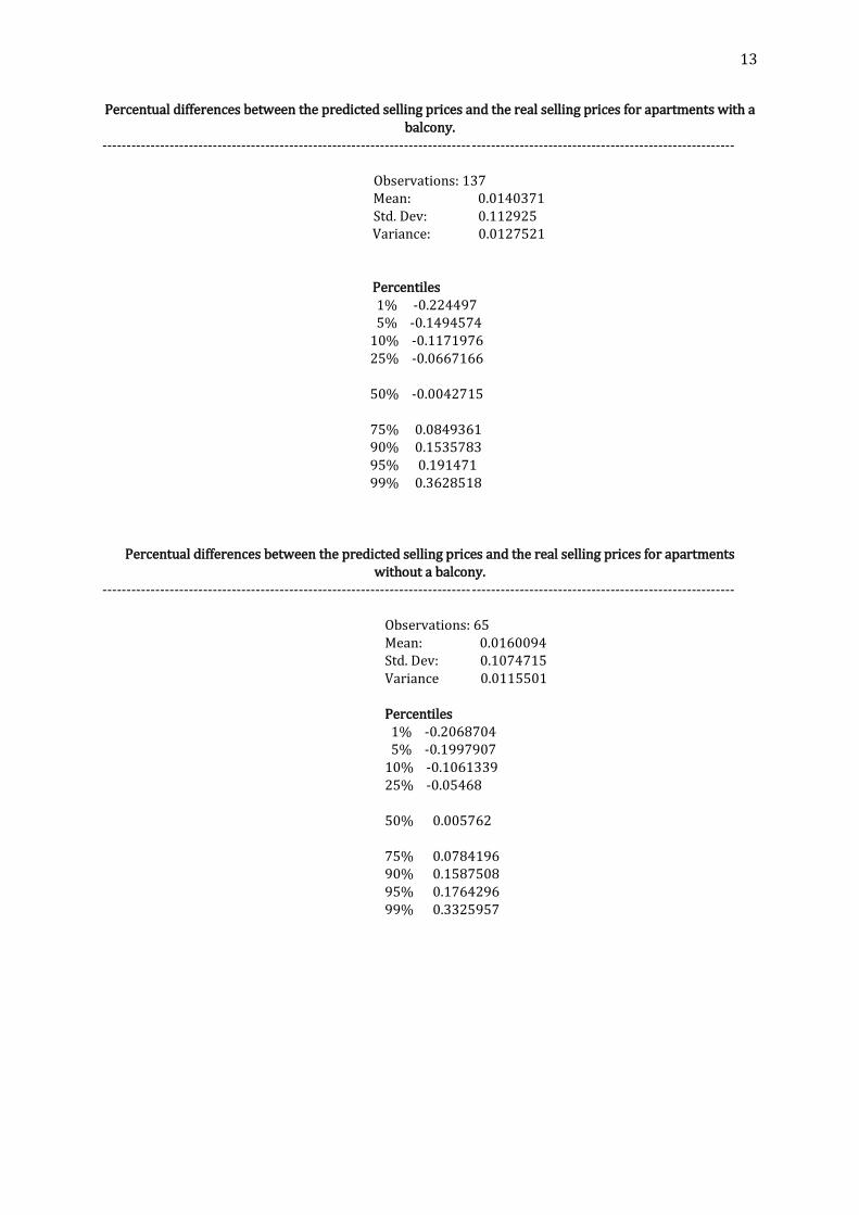
apartments with special conditions are included. First we test the balcony variable. The percental errors for apartment with balconies and the percental errors for apartments without balcony are showed in the tables below.

13

Percentual differences between the predicted selling prices and the real selling prices for apartments with a balcony.

------------------------------------------------------------------------------------------------------------------------------------

Observations: 137 Mean: 0.0140371

Std. Dev: 0.112925 Variance: 0.0127521

Percentiles 1% -0.224497 5% -0.1494574 10% -0.1171976 25% -0.0667166 50% -0.0042715 75% 0.0849361 90% 0.1535783 95% 0.191471 99% 0.3628518

Percentual differences between the predicted selling prices and the real selling prices for apartments without a balcony.

------------------------------------------------------------------------------------------------------------------------------------

Observations: 65 Mean: 0.0160094 Std. Dev: 0.1074715

Variance 0.0115501

Percentiles 1% -0.2068704

5% -0.1997907 10% -0.1061339 25% -0.05468

50% 0.005762

75% 0.0784196 90% 0.1587508 95% 0.1764296 99% 0.3325957

14

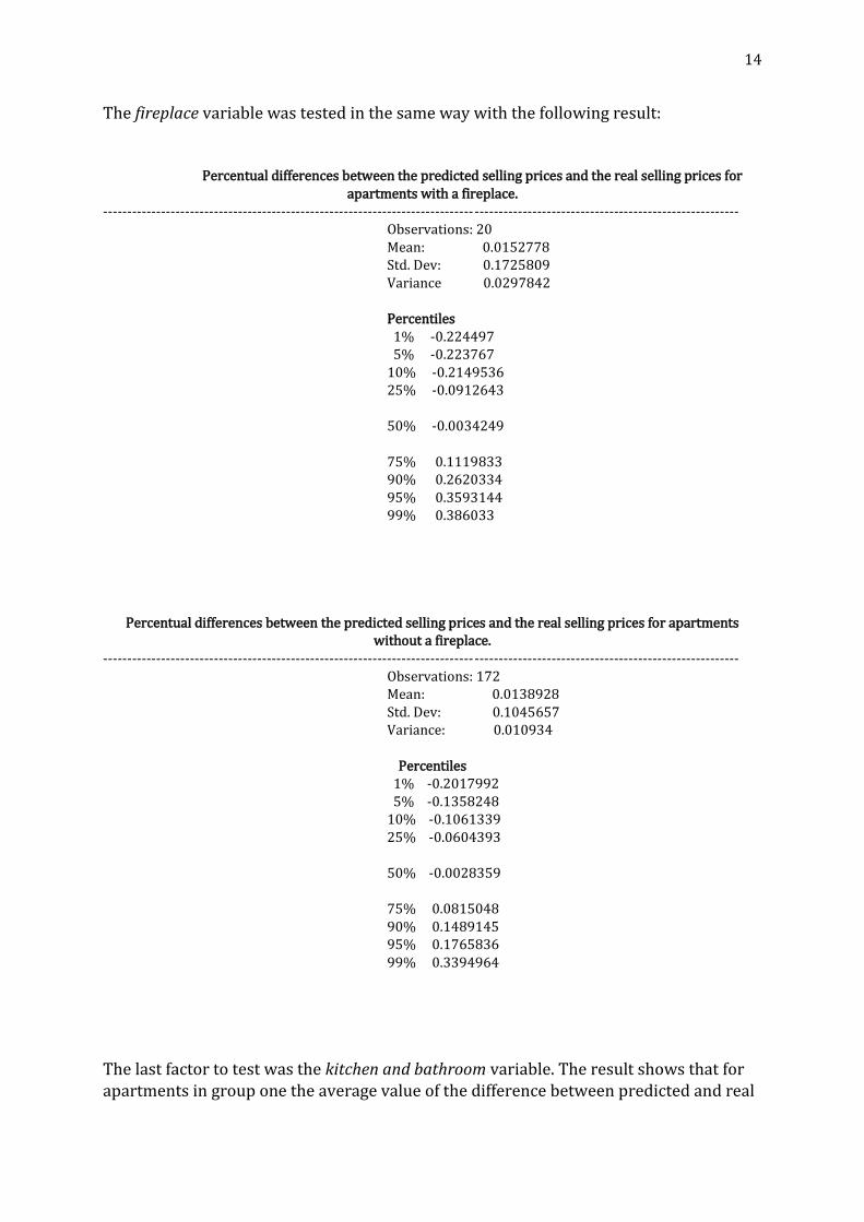
The fireplace variable was tested in the same way with the following result:

Percentual differences between the predicted selling prices and the real selling prices for apartments with a fireplace.

------------------------------------------------------------------------------------------------------------------------------------ Observations: 20 Mean: 0.0152778 Std. Dev: 0.1725809

Variance 0.0297842

Percentiles 1% -0.224497 5% -0.223767

10% -0.2149536 25% -0.0912643

50% -0.0034249

75% 0.1119833 90% 0.2620334 95% 0.3593144 99% 0.386033

Percentual differences between the predicted selling prices and the real selling prices for apartments without a fireplace.

------------------------------------------------------------------------------------------------------------------------------------ Observations: 172 Mean: 0.0138928 Std. Dev: 0.1045657 Variance: 0.010934

Percentiles

1% -0.2017992 5% -0.1358248 10% -0.1061339 25% -0.0604393

50% -0.0028359

75% 0.0815048 90% 0.1489145 95% 0.1765836 99% 0.3394964

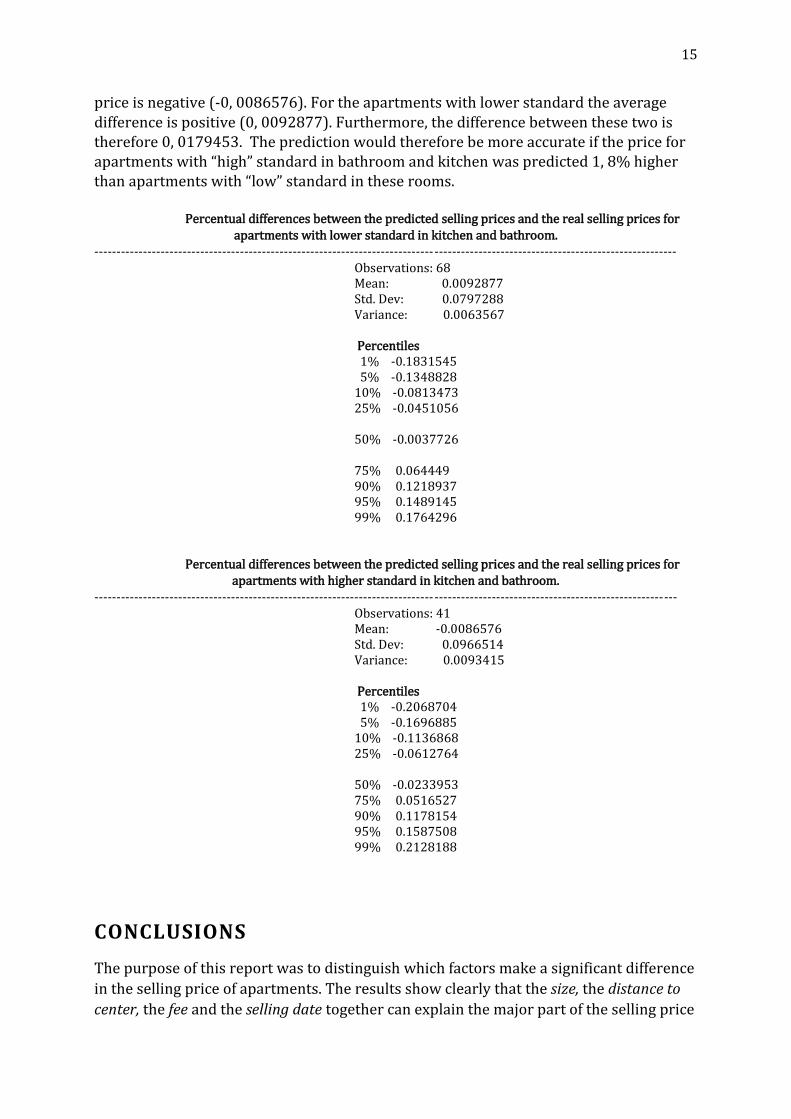
The last factor to test was the kitchen and bathroom variable. The result shows that for apartments in group one the average value of the difference between predicted and real

15

price is negative (-0, 0086576). For the apartments with lower standard the average difference is positive (0, 0092877). Furthermore, the difference between these two is therefore 0, 0179453. The prediction would therefore be more accurate if the price for apartments with “high” standard in bathroom and kitchen was predicted 1, 8% higher than apartments with “low” standard in these rooms.

Percentual differences between the predicted selling prices and the real selling prices for apartments with lower standard in kitchen and bathroom.

------------------------------------------------------------------------------------------------------------------------------------ Observations: 68 Mean: 0.0092877 Std. Dev: 0.0797288 Variance: 0.0063567

Percentiles 1% -0.1831545

5% -0.1348828 10% -0.0813473 25% -0.0451056

50% -0.0037726

75% 0.064449 90% 0.1218937 95% 0.1489145 99% 0.1764296

Percentual differences between the predicted selling prices and the real selling prices for apartments with higher standard in kitchen and bathroom.

------------------------------------------------------------------------------------------------------------------------------------ Observations: 41 Mean: -0.0086576 Std. Dev: 0.0966514 Variance: 0.0093415

Percentiles 1% -0.2068704 5% -0.1696885 10% -0.1136868 25% -0.0612764

50% -0.0233953 75% 0.0516527 90% 0.1178154 95% 0.1587508 99% 0.2128188

CONCLUSIONS

The purpose of this report was to distinguish which factors make a significant difference

in the selling price of apartments. The results show clearly that the size, the distance to

center, the fee and the selling date together can explain the major part of the selling price

16

(77%). One example is when the first test was performed, which included only the size

and the selling date. This test did not only show how big an effect the living area had but also how much the prices changed only between the years 2005-2010.

Other interesting factors that also had an impact on the price were the building year and

the district. The building year itself showed an of 27, 83%. It is worth mentioning

that the building year alone also includes other factors, hence the building year correlates with a lot of other variables. One example is that old apartments are more

often located closer to the center then new ones, therefore the building year may often

include the distance to center and vice versa. This means that it is hard to determinate how much affect each of these variables has. When discovering the effect of different

districts, the same problem occurs. The correlation between the distance to the center

and different districts is very strong. However, this correlation is more interesting. The reason for this is because when both of the variables are included in the regression, the

effect of the district is very clear. According to the test we could determinate that the

district variable explains 6, 79 % of the selling price. Of course the district variable may

also have correlations to other variables. For example; different districts are built in different years and may also be correlated to other variables. These are examples of a general problem when doing a model on something that depends on so many different factors with so many correlations between them; it is hard to state what the variables really test.

Another example of this is the correlation between the streets and the district. Since most of the streets are placed in one or two districts it is hard to conclude which of the variables that actually make an effect. But to exclude one of them is not preferred since both of them together give a better model than if one of them is excluded.

One of the most notable things was how much the number of rooms in two equally big apartments affected the price. One example is that a one room apartment with a selling price of 1000000 SEK would be predicted to 1 040 000 SEK if it would have been split into two rooms. That is, the number of rooms will therefore affect the selling price.

When the best regression was performed, all variables were included from

Mäklarstatistik (size, distance to center, fee, selling date, district, building year, number of

rooms, the street, apartment floor and number of floors in the whole building) and this

resulted in a of 88,87 % and the predicted average error of 10,4%.

Of the three variables that were tested from the prospects; balcony, fireplace and kitchen

and bathroom, only the last variable showed a significant impact on the price. The 1,8 % that differed between the average errors on the predicted apartments with high standard and the ones with low standard seems to be reasonable. Furthermore, the

variables fireplace and balcony did not show a significant effect. For apartments with a balcony a majority was predicted below the selling price and for apartments without balcony it was the opposite. A slight majority of the predictions were then predicted above the selling price. But the difference between the two tables is extremely slight, hence it is hard to state that it is the balcony that makes this difference. The same result was shown when the effect of the fireplace was tested. That the fireplace had such a low

17

effect may have to do with the low amount of observations that had fireplaces (20 out of 192). Why the balcony showed such a lowered significance is harder to give a concrete reason for. That the regression showed such a low effect for the balcony is probably because there are so many excluded variables in that model that have a greater effect on the selling price. Why it is not significant on the prediction test is harder to explain.

DISSCUSSION AND IDEAS FOR FUTURE STUDIES

This is a hot topic and things to explore seem endless. Since there are so many different factors that people have in mind when they buy an apartment, creating a perfect model is probably impossible. However, the number of factors that make a difference is one of the interesting things. By adding more and more variables the model can always be improved. But to find those new variables you need a lot of observations to test them on. The reason for this is that every new variable has such a low impact to the price, and to find a significant effect you need a lot of data. If the purpose is to see the effect of a single variable, it is also very important to make sure that the effect is coming from the tested variable and not from some factor that is excluded in the test. This is hard in this field because of all the correlations between different variables.

When it comes to choosing which variables to test it would be interesting to continue to look at different things in the prospects and find new variables from them. The balcony should have more of an effect then this study showed. But to get a more significant effect, the test should maybe take into consideration that balcony’s varies a lot. They differ in size, standard and which cardinal direction they point at. In new apartments it is also not rare to have more than one balcony which of course may increase the value even more.

The standard in different rooms is also something that people generally think about when they value an apartment. This study only looked at the effect of the standard in the kitchen and the bathroom but of course the other room’s standard may have an effect as well. One interesting thing that was not tested in this study was the construction plans. Is it, for example, worth more to have windows in more than one direction? Is an apartment worth more if it is in the corner of the building? Is a big living room worth more than a big bedroom? Another factor that always can be explored more is the location. It would, for example, be interesting to see if it matters how close you are to certain conveniences such as a food store, a bus stop, or the university etc.

Something that has not been mentioned at all in this study is the effect of the factors regarding the house showing. Do some brokerages tend to raise the price higher than others and does the sex of the broker dealer matter? Is it better to have the house showing on specific days of the week? These variables are, however, hard to use in the purpose of predicting apartments that are still not out for sale, but they may have an effect on the selling price.

18

REFERENCES

Montgomery, D, (2008), “Design and Analysis of Experiments”, Wiley Series.

Draper, N., Smith, H, (1998), “Applied Regression Analysis”, Wiley Series.

Inoune, A., K, Lutz, (2002), “In sample or out of sample tests of predictability which one to use”,

Working series paper.

Dennerheim, H, (2006), ”Prissättningen av bostadsrätter: Vilka faktorer påverkar priserna, vad

är riktpriset för en lägenhet”, Handelshögskolan i Stockholm.

Flodström, A, (2009), ” Prediktion av lägenhetspriser i Stockholm- en statistisk undersökning”,

Stockholms Universitet.

Karlsson, M., Lövgren , (2010), ” Analys av prispåverkande faktorer på bostadsrättsmarknaden

i Uppsala”, Högskolan i Gävle.

http://www.uppsala.se/Upload/Dokumentarkiv/Externt/Dokument/Om_kommunen/Befolkningsutveckling/UppsalaexKN1920-2010.pdf

http://www.uu.se/node97

http://www.valueguard.se