ao-ao86 163 massachusetts inst of tech cambridoe ... · approved =fo puab!c releaas distribution...
TRANSCRIPT
AO-AO86 163 MASSACHUSETTS INST OF TECH CAMBRIDOE OPERATIONS RESE-TC FlS 5/1HIERARCHICAL PROOUCTION PLANNING: A SlINLE STAGE SYSTEM.(U)MAR 80 6 R BITRAN. E A HAAS, A C HAX NOOOI-75-C-0S 6
UNCLASSIF IED TA-17, NL//II"II111
II illflfl IE

LEVEi....... .. '..........................:::: ........... ........ mn.t:.4:ij~;:j 5 .~l:~ r. 5
HIERARCHICAL PRODUCTION PLANNING:A SINGLE STAGE SYSTEM
4 ~ I byGABRIEL R. BITRAN,
ELIZABETH A. HAASGc~I and
ARNOLDO C. HAX........... ...
DTICTechnical Report No. 174 JUL 1 Ta
OPERATIONS RESEARCH CENTES A D
I IST92mBUAm.fAEEIA
Approved =fo puab!c releaasDistribution Uniitdc
MASSACHUSETTS INSTITUTEor
TECHNOLOGY
March 1980
80 6 30 157
( HIERARCHICAL PRODUCTION PLANNING:
A SINGLE STAGE SYSTEM,
by
/0 GABRIEL R./DITRAN
ELIZABETH
-ARNOLDO /lHA
Technical Wipt No. 174
j5) Work Performed Under
Contrac N 0'014-75-C-056, Of fice of Naval Research
Mut eve o Loistics Organization Models
Project No. NR 347-027 .-. Fr
Operations Research Center
Massachusetts Institute of Technology
Cambridge, Massachusetts 02139
/1 MarM84 .Y' CO4 9 3
and! /c.Reproduction in whole or in part is permitted for any purpose of the
United States Government.

UnclassifiedSECURITY CLASSIFICATION OF THIS PAGE M%411 DIN& E2mIer ________________
REPORT DOCUMENTATION PAGE 3EOE COuPLrMG oin1. REPORT HUMMER 2. 30VT ACC95SPON NO0 S, RECIPIENT'S CATALOG N$UMDER
Technical Report No. 174 0
S. TITLE (and Iabtttt) a. TYPE OF REPORT 0 PERIOD COVERCo
HIERARCHICAL PRODUCTION PLANNING: A SINGLE Marchnia Repor
STAGE YSTEMS. PERFORMING ORG. REPORT NUMBER
7. AUTNOR(e) 41. CONTRACT OR GRANT NUMBERfe)
Gabriel R. Bitran N00014-75-C-0556Elizabeth A. HaasArnoldo C. Hax ______________
SPERFORMING ORGANIZATION NAME AND ADDRESS 10. PROGRAM ELEMENT. PROJECT. TASKCAREA & WORK UNIT NUMBERS
M.I.T. Operations Research Center77 Massachusetts Avenue NR 347-027Cambridge, Massachusetts 02139 _______________
I1. CONTROLLING OFFICE NANE AND ADDRESS 12. REPORT DATE
O.R. Branch, ONR Navy Department March 1980
800 North Quincy Street 1 pagBEsFPAEArlington, VA 22217 41 pages___________
WS. MONITORING AGENCY NAME S ADORESS(if dfeent ine Controlling Offloe) IS. SECURITY CLASS. (of ti repot)
15a. OECL ASSI FICATIONIDOWNGRADINGSCHEDULE
IS. DISTRIBUTION STATEMENT (of tis Report)
Releasable without limitation on dissemination.
17. DISTRIBUTIOH STATEMENT (of the sbettedt entered in Block 20, It different from, Report)
IS. SUPPLEMENTARY NOTES
is. KEY WORDS (Continue on reverse eide it neceeeay end identify by Weoek nsumber)
Aggregate Production PlanningProduction PlanningDisaggregation
20. ABSTRACT (Continue ont reverse side If neceesey and Identify by block number)
See page ii
D iJAwn 1473 EDITION OF INov 66 is OBSOLETE UnclassifiedSECURITY CLASSIFICATION OF THIS PAGE (USmIa Date Etrd
ii
FOREWORD
The Operations Research Center at the Massachusetts Institute of
Technology is an interdepartmental activity devoted to graduate education
and research in the field of operations research. The work of the Center
is supported, in part, by government contracts and grants. The work re-
ported herein was supported by the Office of Naval Research under Contract
No. N00014-75-C-0556.
Richard C. Larson
Jeremy F. Shapiro
Co-Directors
ABSTRACT
This paper presents a hierarchical approach to plan and schedule
production in a manufacturing environment that can be modelled as a
single stage process. Initially, the basic trade-offs inherent to
production planning decisions are represented by means of an aggregate
model, which is solved on a rolling horizon basis. Subsequently, the
first solution of the aggregate plan is disaggregated, considering
additional cost objectives and detailed demand constraints.
Several improvements in the methodology related to hierarchical
production planning are suggested. Special attention is given to
alternative disaggregation procedures, problems of infeasibilities, and
the treatment of high setup costs. Computational results, based on real
life data, are presented and discussed.
31

1. INTRODUCTION
In this paper we will concentrate exclusively on the design of model-
based systems to support tactical and operational decisions pertinent to
production planning. Tactical decisions are concerned with the allocation
of the resources available for production purposes. Typical decisions are
the amounts of each product type to be produced in each period, the levels
of regular and overtime workforce to be used, specification of service
levels, inventory targets, machines capacities, etc. An appropriate
planning horizon for these decisions is a full seasonal cycle to capture
the fluctuations in demand due to seasonalities and promotions. The
length of the cycle is usually one year. To make effective tactical deci-
sions it is generally sufficient to consider aggregate data. The basic
operational decisions of production planning consist in establishing the
amount of each item that must be produced in each period and the correspond-
ing resources needed. Operational decisions are made subject to the limita-
tions imposed by the tactical level and require a high degree of detailed
information.
In many practical situations of batch processing systems, tactical and
operational decisions are taken by distinct managerial echelons. This
fact must be recognized by system designers if an implementation is to
succeed. Although production planning has attracted the attention of
operation researchers for a long time, the different nature of the two
classes of decisions mentioned above has been seldomly considered. Some
exceptions include the works of Holt, Modigliani, Muth and Simon [161,
Winters [27], Hax and Meal (15], Bitran and Hax [2], Shwimer [231, Newson
[21], and Zoller [28]. However, most publications encountered in the
literature either formulate the production planning problem at a detailed
level, [71,[8],[19],[201, or advocate an aggregate approach and give little

Ii
-2-
insight into how to disaggregate the solutions, see [4],[5],[ll],[18], and
[251. The detailed formulation of the problem leads to a very large mathe-
matical programming problem which is very difficult to interact with, requires
demand data that can seLdomly be forecasted with an acceptable accuracy, and
is expensive to operate.
In this paper we present an improved version of the hierarchical proce-
dure for production planning suggested by Bitran and Hax [2] and provide
theoretical results supporting the method. To make this paper as self
sufficient as possible we briefly describe the hierarchical production
planning concept.
1.1 Hierarchical Production Planning
Hax and Meal introduced the concept of hierarchical production planning
in [15]. The method consists primarily of recognizing the differences
between tactical and operational decisions. The tactical decisions are
associated with aggregate production planning while the operational deci-
sions are an outcome of the disaggregation process.
Hax and Meal proposed the following levels of aggregation:
Items: are the end products delivered to customers.
Product Types: are groups of items having similar unit costs, direct costs
(excluding labor), holding costs per unit per period, productivities
(number of units that can be produced per unit of time), and season-
alities.
Families: are groups of items pertaining to a same product type and sharing
similar setups. That is, whenever a machine is prepared to produce
an item of a family, all other items in the same family can
also be produced with a minor change in setups.Although we have adopted this three-level product structure in our
-3-
work, the reader should realize that a specific disaggregation hierarchy
depends on the actual setting being considered.
An overview of hierarchical production planning is shown in Figure 1.1.
It applies to single stage batch production processes. An extension for
Multistage processes is given in [1]. As indicated in Figure 1.1, three
levels, paralleling the aggregation hierarchy, are recommended (boxes 1, 2,
and 3). The first is the product type level where aggregate plans for
product types are determined. The planning horizon is usually one year.
This level is concerned with tactical decisions. Only the amount of each
product type to be produced in the first period is passed to the family
level (box 2). Aggregate production plans are determined on a rollinF
horizon basis. That is, the planning horizon is maintained equal to one
year by deleting the last period and adding a new one. At the second level
the run quantity of each type is disaggregated to obtain the production
quantities of each family. These are passed to the item level (box 3) where
they are further disaggregated to determine the amount of each item to be
produced in the first period. It is important to notice that in the hier-
archical method detailed forecasts at the item level over the entire aggregate
p lanning horizon are not needed. As a consequence, the data collection
required is considerably smaller than in detailed formulations of the
production planning problem. Moreover, the fact that there are usually a
few numaber of product types justifies the use of sophisticated forecasting
techniques that would be prohibitively expensive to employ for thousands
of items. Since aggregate forecast tends to be more accurate than detailed
forecast, production plans generated by hierarchical planning tend to be
quite stable in the rolling horizon process.
Hax and Meal proposed a heuristic to perform the three levels (boxes 1,
2, and 3) in Figure 1.1. flitran and Ham formalized the hierarchical planning

! I
-4-
Read in last period's usage
Ia,Update Inventory Status
(Physical Inventory, Amount onOrder, Backorders, Lost Sales,
Available Inventory)
Update demand forecasts, safetystock. overstock limits, and
run out times
Determine effective demandsfor each product type*
a Aggregate Plan for Types ()
(Aggregate Planning Reports)
(3)kItem Disaggregation t
(Item Planning Reports)
Detailed Status Reports
Figure 1.1: Conceptual Overview of Hierarchical Planning System
For a discussion of effective demands, see Section 2.2.
___ ___ ___ __ _ _ ___ ___ _ ... ,t 7 -~ ___4_

heuristic by suggesting the use of convex knapsack problems to disaggregate
the product type and families run quantities into families and item run
quantities, respectively.
The plan of the paper is as follows. In section 2 the algorithm
suggested by Bitran and Hax is briefly reviewed. In section 3 theoretical
results supporting the hierarchical production planning method are provided.
Three modifications to the algorithm in [23 are introduced in section 4.
Results of extensive computational experiments comparing several hierarchi-
cal procedures are given in section 5. Conclusions are presented in
section 6. Proofs of the theorems are presented in the appendices.
-6-
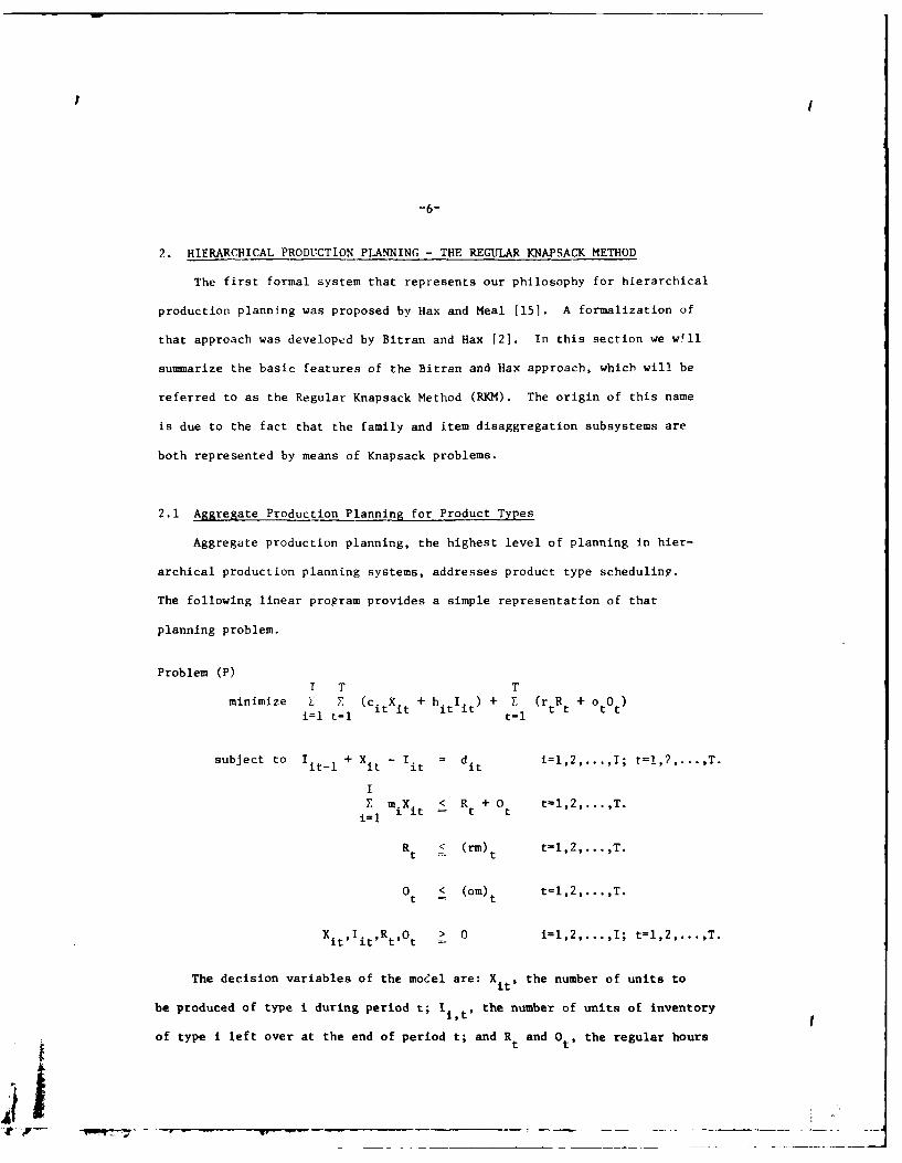
2. HIERARCHICAL PRODUCTION PLANNING - THE REGULAR KNAPSACK METHOD
The first formal system that represents our philosophy for hierarchical
production planning was proposed by Hax and Meal [151. A formalization of
that approach was developed by Bitran and Hax [2]. In this section we will
summarize the basic features of the Bitran and Hax approach, which will be
referred to as the Regular Knapsack Method (RKM). The origin of this name
is due to the fact that the family and item disaggregation subsystems are
both represented by means of Knapsack problems.
2.1 Aggregate Production Planning for Product Types
Aggregate production planning, the highest level of planning in hier-
archical production planning systems, addresses product type scheduling.
The following linear program provides a simple representation of that
planning problem.
Problem (P)I T T
minimize Z Z (citXit + h itlit) + E (rtR t + ot0)il it=l t=l
subject to I itl + Xit - Iit dit i=l,2,...,I; t=!,?,...,T.
I
E miX it< R + 0 t=l,2,...,T.i=l
Rt < (rm) t t-l,2,.....T.t t
0t < (om)t ~ , ... T
XitIitRt9Ot > i=l,2,...,I; t=l,2,...,T.
The decision variables of the moeel are: Xit, the number of units to
be produced of type i during period t; I i t , the number of units of inventory
of type i left over at the end of period t; and Rt and Or, the regular hours

-7-
and the overtime hours used during period t, respectively.
The parameters of the model are: T, the length of the planning horizon;
c i, the unit production cost (excluding labor); hit, the inventory carrying
cost per unit per period; rt and ot, the cost per manhour of regular labor
and of ove-time labor; (rm)t and (om) t, the total availability of regular
and overtime hours in period t, respectively; mi, the hours required to
produce one unit of product type i; and dit, the effective demand for
type i during period t. (A definition of effective demand is given below.)
For simplicity of presentation, we have not incorporated in Problem (P)
hiring and firing, production lead time, backorders and other features
that can be easily considered. Moreover, the aggregate Problem (P) need
not necessarily be formulated as a linear programming problem. Any
aggregate production planning model may be used as long as it adequately
represents the practical setting under consideration. Discussions of
aggregate models can be found in [12],[6],[22], and [17]. Problem (P)
is solved with a rolling horizon of length T. At the end of every time
period, new information becomes available and is used to update the values
of the parameters of the model, particular demand forecasts, and the result-
ing values of the decision variables. Due to the uncertainties present
in the planning process, only first period results of the aggregate problem
are actually implemented.
2.2 Effective Demand
As is shown in Bitran and Hax [21, the use of demand, instead of
effective demand, may lead to an aggregate solution of Problem (P) which
cannot be disaggregated. The effective demand represents net requirements
which cannot be satisfied from initial available inventory. More precisely,
let Iko represent the initial inventory of item k, and dkt denote the demand
I,-L__- _ __ ___ __ ___ _.__
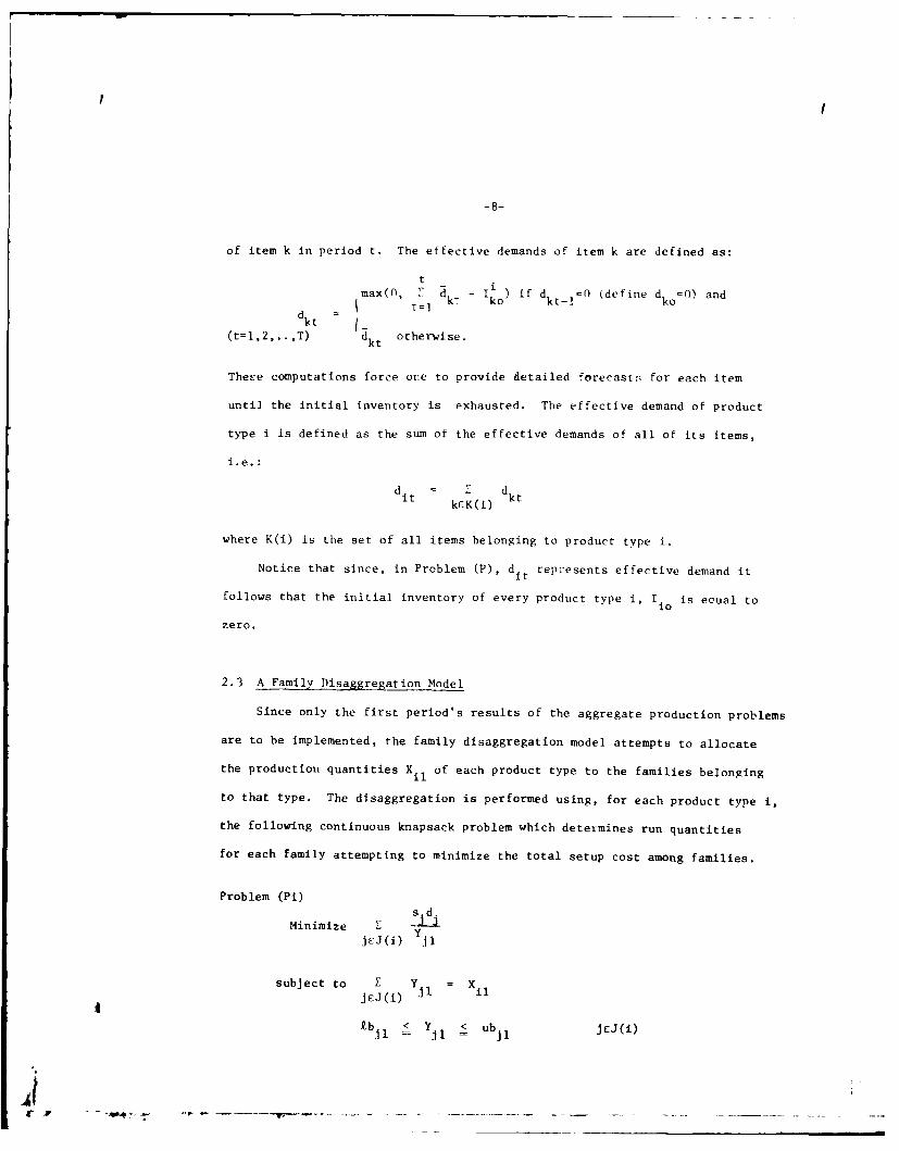
-8-
of item k in period t. The effective demands of item k are defined as:
t - imax(O, . d - I ) if d 0 (define d =0) anddk ko kt-1 ko
dkt
(t=l,2,..,T) dkt otherwise.
Theve computations force one to provide detailed forecasts for each item
until the initial inventory is exhausted. The effective demand of product
type i is defined as the sum of the effective demands of all of its items,
i.e.:
d dkEK(i) kt
where K(i) is the set of all items belonging to product type i.
Notice that since, in Problem (P), dt repiesents effective demand it
follows that the initial inventory of every product type i, Iio is equal to
zero.
2.3 A Family Disaggregation Model
Since only the first period's results of the aggregate production problems
are to be implemented, the family disaggregation model attempts to allocate
the production quantities Xil of each product type to the families belonging
to that type. The disaggregation is performed using, for each product type i,
the following continuous knapsack problem which determines run quantities
for each family attempting to minimize the total setup cost among families.
Problem (Pi)
Minimize Z
jEJ(0) Yjl
subject to E Y = XJrJ(i) YJl Xil
kb < Y < ub JEJ(i)=i •I !i
2 A

-9-
where s. and d denote the setup cost and annual demand of family J. The
variables Yjl represent the quantity to be produced of each family j during
period 1. The upper bound ub j and lower bound Zb j are computed as follows:
ub = max(O, OS - a ji ) and
Zb j = max(0, djl -aijl + ss j)
where osjl, djl, aijl and ss j denote respectively the overstock limit,
the demand, the available inventory, and the safety stcck of family j in
period 1. J(i) is the set of families in product type i that trigger in
period 1, i.e., it is the set of indices j such that djl - aiji + SSjl > 0.
The objective function of Problem (Pi) assumes that the family run
quantities are proportional to the setup cost and the annual demand for a
given family. This assumption, which is the basis of the economic order
quantity formulation, tends to minimize the average annual setup cost. In
section 4.1 this objective function will be reviewed. An efficient algorithm
to solve Problem (Pi) is given in Bitran and Hax [2].
2.4 The Item Disaggregation Model
Once the quantities Y have been determined, one needs to disaggre-
gate them among the items belonging to each family J. For the current
planning period, all costs have already been determined by the two previous
stages in the hierarchical process. However, the feasible solution chosen
will establish the intial conditions of the next period and will affect
future costs. In order to save setups in future periods, it seems reason-
able to distribute the family run quantity among its items in such a way
that each item's runout time coincides with the runout time of the family.
This can be accomplished by the following continuous knapsack problem.
-7
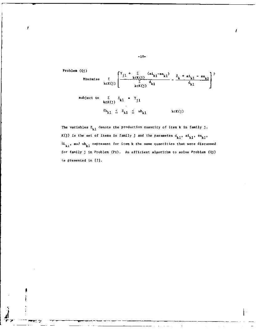
Problem (QJ) rYJ + E (al-ss) 881 2Minimize r kEK(j) ilkl Zk + aik
kEK(j) [EJ dkl dkl
subject to E = Yk jkcK(J) z k
Zb <Z < bkK)kl =Zkl Ubkl kcK(J)
The variables Z denote the production quantity of item k in family J.
K(j) is the set of items in family j and the parametes dkl , aikl, aSkl'
4Lki, auJ ubkl represent for item k the same quantities that were discussed
for family j in Problem (Pi). An efficient algorithm to solve Problem (Qj)
is presented in [2].
if_ _ _ _ _ _ _ _ _ _ _ _ _ _
[ ~ - - _ _ _ _ _ __ _ _ _ _ _ _

-Ii-
3. COMPARING DISAGGREGATION PROCEDURES
An important determinant for the performance of hierarchical production
planning systems is the procedure used to disaggregate earlier decisions at
each hierarchical level. The knapsack approach just presented identifies one
possible alternative for hierarchical designs. The knapsack nature of the
subproblems is very appealing because of its great computational advantage.
However, it is imperitive that we gain some theoretical understanding of
the impact of different disaggregation schemes on the production planning
costs. Such an understanding will help us in evaluating and comparing
alternative disaggregation mechanisms, and in judging the improvements to
be obtained by introducing modifications to the RKM.
This section will describe two fundamental theorems which provide
important insights into the strengths of various disaggregation methodolo-
gies. Let the superscript u denote a generic disaggregation procedure
applied to Problem (P). The effective demands can be expressed as a funczion
of the real demands (or forecasted demands) and the disaggregation procedure
used as follows:
d = di -gU for i=i,2,...,I and t-1,2,...,T.it it i
The quantity gut represents the total contribution of all items belonging
to product type i to determine the effective demand of that product type
in period t, using the disaggregation procedure u. Different disaggregation
procedures will affect the initial inventory of each item and, thus, theT
ueffective demand of the product types. Therefore, E gut, T-l....,T indicate
t.1the suim of the real or forecasted demands of the items in product type i that
can be satisfied directly by the initial inventory up to period T.
Problem (P) can be rewritten as a function of disaggregation u as
follows:
• ,____ ______________

-12-
Problem (PU)
I T Tmin E E (C tXt + hI ) + Eo t
) u
i=l t=1 t=l
I T-1 T+ E E ht u
i=l t=l k=t+l
subject to li + X - I = d t =1'2"'"I; t1,2,...,T.it-I it -i t it i
I
m Xu < Ru +0u t=l,2,...,T.i it t t
Ru < (rm) t=l,2,... ,T.t t
Ou < (o,) t=l,2,... ,T.t = t
Xu u Ru Ou >
it' itR t0 t - 0
where the last term in the objective function represents the holding enmt
of the initial inventory of all product types, which is a function of the
disaggregation procedure used. This term has been omitted in Problem (P)
since, given a disaggregation procedure, the initial inventory cost is
constant. However, it is important to include it in Problem (pU) because
our purpose is to compare the performance of various disaggregation proce-
dures.
The quantities git satisfy the following condition
T
t=l i io
where lio is the initial inventory of product type i.
A disaggregation procedure u is said to be feasible if Problem (PU)
is feasible.
I
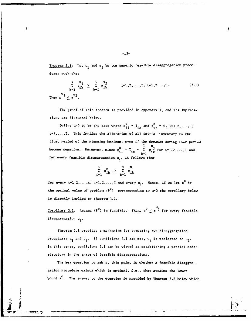
-13-
Theorem 3.1: Let u1 and u2 be two generic feasible disaggregation proce-
dures such that
t uI t u2Egik > E g ik i-1,2,...,1; t=1,2 ....,T. (3.1)
k-1 k-i
Then z < z
The proof of this theorem is provided in Appendix 1, and its implica-
tions are discussed below.
Define u=O to be the case where g = 1 and = 0,
t-2,... ,T. This inrklies the allocation of all initial inventory to the
first period of the planning horizon, even if the demands during that periodT u.
become negative. Moreover, since g 1 Z g J for i=1,2,...,I andil io k=1li
for every feasible disaggregation u,, it follows that
t t U.F o > X g Il gik = k
1=1 k=l
for every t=l,2,...,t; i=1,2,...,l and every u. Hence, if we let z0 be
the optimal value of problem (P0 ) corresponding to u=0 the corollary below
is directly implied by theorem 3.1.
u
Corollary 3.1: Assume (P0 ) is feasible. Then, z° < z J for every feasible
disaggregation uj.
Theorem 3.1 provides a mechanism for comparing two disaggregation
procedures u1 and u2 . If conditions 3.1 are met, u1 is preferred to u2.
In this sense, conditions 3.1 can be viewed as establishing a partial order
structure in the space of feasible disaggregations.
The key question to ask at this point is whether a feasible disaggre-
gation procedure exists which is optimal, i.e., that attains the lower
0bound z . The answer to the question is provided by Theorem 3.2 below which
p.i

-14-
establishes the conditions under which the disaggregation procedure known
as "Equalization of Run Out Times" (EROT) becomes optimal.
EROT allocates the production amount determined at the aggregate
planning level for a given product type, Xti, in such a way as to equal-
ize the run out times of all the items belonging to that type. The run
out time for a product type is defined as the nuber of periods (possibly
a fractional number) that will elapse until the inventory of that item
reaches the safety stock level.
Theorem 3.2: Let uE denote the EROT disaggregation procedure. Then, if
all disaggregations are made with the EROT disaggregation method, if
Iin > 0 for all product types, and if the aggregate product type problem
(Po) is feasible it follows that
0 uE
The proof to this theorem is provided in Appendix 2.
ReEbiniziag that the aggregate plan ignores setup costs, there are
two important conclusions that are derived from Theorems 3.1 and 3.2.
First, a qualitative interpretation of Theorem 3.1 is that the
larger the gat's are for small values of t, the better it is in terms
of total primary costs. That is, the best disaggregation scheme must
allocate the initial inventory of e*ch product type uniformly, in
terms of runout time, among all its items. This interpretation makes
clear that the EROT disaggregation is optimal, as proved in Theorem 3.2.
however, when setup costs grow in importance it is desirable to allocate
larger inventories to the items that have the highest setup costs. The
motivation for a non-uniform allocation of inventories among items in a
product type is the desire to minimize total setup costs. Therefore, we
face a tradeoff between using the EROT disaggregation procedure and coae-
-7- V.-'

-15-
quently minimizing total primary costs while incurring high setup costs,
and choosing a disaggregation that allocates the inventories in a manner
that considers setup cost levels reducing these costs while incurring higher
primary costs. Our computational experience, to be discussed in section 5,
has shown that when the total setup costs are 5% or less of the total produc-
tion costs, EROT performs quite efficiently. The RKM, enhanced by modifica-
tions to be introduced in the next section, is one of those methodologies
that are more effective than EROT when setup costs are significant.
Second, EROT is a "myopic" disaggregation rule. The aggregate planning
model covers a long planning horizon, usually a full year, to allow for an
efficient allocation of facilities, manpower, and inventory under fluctuating
demand conditions. However, once the aggregate plan has been established,
we need just to look for a few periods ahead (the length of which is repre-
sented by the runout time) to determine an appropriate disaggregation.
Although EROT is an optimal disaggregation procedure only under the absence
of setup costs, the qualitative implications of this approach support the
essence of hierarchical planning, that advocates the use of long planning
horizons at the highest planning level, while drastically decreasing the
planning horizons at the lower planning levels.
f _ _ _ _ _ _ _ __ _ _

-16-
4. MOlIFICATIONS INTRODUCED IN THE REGULAR KNAPSACK METHOD
The concerns about the performance of disaggregation procedures under
high setup costs, and the myopic nature of disaggregation rules, led us to
incorporate modifications in the Regular Knapsack Method. Computational
results evaluating the performance of EROT, RKM, and the modified Knapsack
will be presented in section 5. This section will cover three important
changes made to RKM.
4.1 A Myopic Objective Formulation for the Family Subproblem
The objective function proposed originally in the RKM (see section 2.3)
was:
Minimize E YJEJ(i) jl
The definition of d., covering demand over the entire planning horizon,j
contradicts the myopic nature of the disaggregation process referred to in
the previous section. As a consequence, the resulting solutions YJl of
Problem (Pi) will not be sensitive to the difference among the demand
patterns of the families belonging to a given product type in the immediate
future. Inspired by the results of Theorem 3.1 and 3.2, d was redefined
as a demand for family j over the run out time of its corresponding product
type; that is to say, over the time interval that would exhaust the produc-
tion quantity Xil of the product type i containing family j when that quan-
tity is disaggregated according to the EROT scheme.
4.2 The Look Ahead Feasibility Rule
Another important problem that led us into modifying the RKM was the
generation of infeasibilities that could be introduced in the aggregate
problem by the disaggregation procedure used. Golovin [10] detected this
"---'7 ---- -- -------,--___ ___-_ __ __
-17-
problem and illustrated its occurance by means of a numerical example.
Gabbay [9] suggested a set of constraints to be introduced in the family
subproblem that would provide necessary and sufficient conditions for the
existence of feasible disaggregations over the entire planning horizons.
His results, however, were restricted to the static case; that is, when
Problem (P) is solved only at the beginning of the first period and no
rolling horizon is used. Moreover, Gabbay's constraints destroy the s~ecial
knapsack structure of the family subproblems, thus eliminating the c)inpu-
tational advantages of such a structure.
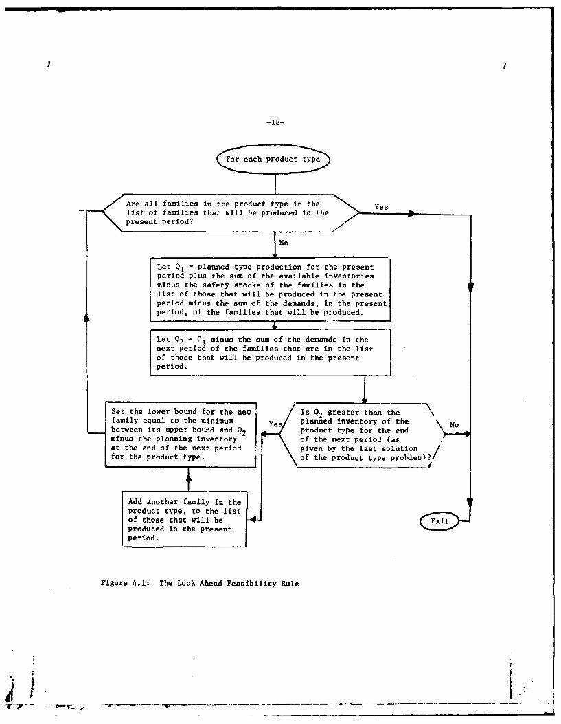
To overcome the potential presence of infeasibilities, we developed
a simple rule that looks ahead just one period, attempting to prevent the
next period's disaggregation from becoming infeasible. We designated this
rule as the "Look Ahead Feasibility Rule". The essence of the computations
needed to carry out this rule is presented in Figure 4.1.
A numerical example might facilitate an understanding of the applica-
tions of this rule.
Assume that the aggregate schedule for product type P1, composed by
families Fl and F2, is:
Product type P1: Initial Inventory Production Demand Ending Inventory
Period 1 10 units 25 units 20 units 15 units
Period 2 15 units 5 units 20 units 0 units
Demand and inventory data for families Fl and F2 are as follows:
F1 F2
Initial inventory in period 1 0 units 10 units
Demand in period 1 10 units 10 units
Demand in period 2 10 units 10 units
The inventory figures do not include safety stocks.
'V -7 ,_ _ _ _ _ _ _ _ ___,
-18-
t f ih
product
typ e
< Are all families in the product type in the > Yes
- list of families that will be produced in the
present period?
Let Q, = planned type production for the presentperiod plus the sum of the available inventoriesminus the safety stocks of the families in thelist of those that will be produced in the presentperiod minus the sum of the demands, in the presentperiod, of the families that will be produced.
Let Q2 = 01 minus the sum of the demands in thenext period of the families that are in the listof those that will be produced in the presentperiod.
Set the lower bound for the new Is Q2 greater than thefamily equal to the minimum planned inventory of thebetween its upper bound and 02 product type for the endminus the planning inventory of the next period (as
at the end of the next period given by the last solution /
for the product type.k of the poduct type proble)?/
Add another family is the
product type, to the list
of those that will be -4itproduced in the presentperiod.
Figure 4.1: The Look Ahead Feasibility Rule
-9 - -- -- --- " --- .....

-19-
According to this data, only Fl will trigger in the first period.
Therefore, under RKM, only Fl will be produced and its production quantity
will be 25 units (for simplicity, we are assuming no upper bounds for both
families). In the second period, only F2 will trigger, since its initial
inventory will be zero units and its demand will be 10 units. However,
since the production scheduled for PI is 5 units, a shortage of 5 units for
family 2 will results. If the Look Ahead routine in Figure 4.1 is applied,
the value of Q1wlbeQ=2501=15adQ2= 15-10 = 5. The planned
inventory for the product type P1 at the end of period 2 will be zero units.
Hence, Q2= 5 > 0. Therefore, the "look ahead feasibility rule" adds to
the list of families to be produced in the present period (period 1), composed
just by Fl, the family F2 with a lower bound of 5 units for its production
quantity. This modification will eliminate the infeasibility created by
RICH. It is important to note that this adjustment routine does not preclude
the use of the efficient knapsack algorithm to solve the family subprobleri (Pi).
4.3 Modification of the Regular Knapsack Method for the Case of High Setup Costs
We have already addressed the role of setup costs in hierarchical produc-
tion planning systems. The initial approaches introduced by Hax and Meal (15]
and Bitram and Hax [2] ignore the setup costs at the product type level, and
include them in the decision rules at the family level. The resulting
algorithms proved to be effective when setup costs did not exceed 10 percent of
the total production costs (for further discussion of this subject see [21,(141).
The issues that still deserve consideration are those cases in which
setup costs represented a percentage higher than 15 of the total production
cost. Figure 4.2 describes a subroutine that we introduced to the RICH for
those situations with fairly high setup costs. This routine can be easily
modified to allow for managerial inputs which reflect their Judgment regard-

!I
-20-
For each product type isolve the family subproblem
(Pi)
For each family J, compute the integer number of periods, N(J),of demand that can be satisfied with the production quantity yjiallocated to the family by subproblem (Pi).
For each family J, compute the "ideal production quantity", usingSilver-Meal lot sizing procedure [24], and the associated integernumber of periods, M(j), of demand that can be satisfied by thisproduction quantity.
For each family J, free the production capacity corresponding toproducing more than min [N(j); M(j)] periods of demand.
Let CAP denote the sum of the production capacities freed by eachfamily independently of the product type it belongs to.
Allocate the capacity CAP to the family(ies) in quantities equalto full periods of demand, whenever possible, in such a way to"rminimize the total production costs".
4If the aggregate problem (P) did not use all regular hours ofproduction in the present period, treat this extra capacity asfree capacity and allocate it to some family(ies) as long as ithas a positive impact on the total costs.
Figure 4.2: Routine to Adapt the RKM for the Case of High Setup Costs
t , - !-- 7 . . .... .. . .. . .. ...... .
-21-
ing changes to be incorporated in the aggregate schedule in order to save
setup costs. These changes will invariably represent tradeoffs between
the linear costs identified in the aggregate production level and the setup
costs incurred at the family level.
The routine briefly described in Figure 4.2 works as follows. Ini-ially
the family subproblems (Pi) are solved and the production quantities Yjl
for each family are obtained. The integer number of periods of demand, or
each family J, that can be satisfied by YJl is computed and denoted by N,J).
Next, Silver-Meal's lot sizing method [241 is applied, for each family j.
considering the stream of demands starting with the present period. The
otuput of the method is denoted by L(j) and we refer to it as the ideal
quantity to be produced for family j in the present period. We have chosen
Silver-Meal's procedure instead of the Wagner-Whitin [261 algorithm because
the first is much more efficient computationally and gives satisfactory
results (see [221 for a comparison of the two methods). The next step is
to compute the integer number M(j) of periods of demand that can be totally
satisfied by L(j). It is important to note that N(j), L(j), and M(j) are
computed considering effective family demands. For each family, the differ-
ence between the capacity allocated by the family subproblems and the
capacity needed to cover the demand for more than minimum [M(J),N(j)] periods
is considered freed. The sum of the freed capacities of each family,
independently of the product type to which it belongs, is denoted by Z.
After removing the free capacity from each family, we denote the remaining
production quantity by Q(J). All families are ordered according to1 sjdj hiQ(i)
"increasing marginal costs", MC(J) = - -.1 --( 2 , where s is
the setup cost for family J, d is the demand of family j over the myopic
planning horizon (as defined in section 4.1), and hi is the cost of holding
one unit in stock for one period. The capacity Z is then allocated to the
-22-
families in quantities equal to full periods of demand (whenever possible,
.,1* t. Me* V estarting with the one with minimum MC(j)). After allocating one period of
demand to a family J, its marginal cost is recomputed witi Q(j) increased
by the corresponding amount. If after allocating the capacity Z there
exists at least one family with negative marginal cost, and there are
regular hours of production available, that the aggregate problem (P) did
not use for the present period, the routine allocates the time available
to those families. We would like to point out that variants of the marginal
criterion, MC(j), have been tested and none performed better than the one
reported here. This approach effectively alters the aggregate schedule as
long as the expected savings in setup costs more than compensate for
changes in the costs considered by the aggregate schedule.
4' .

-23-
5. COMPUTATIONAL RESULTS
A series of experiments were conducted to examine the performance of
the modifications introduced in the hierarchical knapsack method and to
compare this method with others. The data used for these tests was taken
from a manufacturer of rubber tires. The product structure characteristics,
together with relevant information, are given in Figure 5.1. The twelve
items were partitioned into two product types P1 and P2. Product type P1
is composed by two families PlFl and P2F2. The second product type is
partitioned into three families P2Fl, P2F2, and P2F3. Table 5.1 exhibits
the demand pattern for both product types.
The experiments were divided in two sets. In the first set, they
consisted of applying the production planning methods to a full year of
simulated plant operations. Production decisions were made every four -eeks.
The model was then updated using a one year planning horizon. The process
was repeated thirteen times. At the end of the simulation, total setup costs,
inventory holding costs, overtime costs, and backorders were calculated.
Direct manufacturing costs and regular work force costs were omitted because
they were considered fixed costs for this applications.
The methods compared are:
1) The RKM modified by considering the myopic horizon for the demand at
the family level (subsection 4.1) and the "look ahead feasibility
rule" (subsection 4.2). In Table 5.2 this method corresponds to
the column K12.
2) The RKM with the three modifications, i.e., the modifications considered
in 1) above, plus the adjustment routine for high setup costs
(subsection 4.3). In Table 5.2 this method corresponds to the
column K123.
3) EROT which consists in disaggregating the product type production quanti-
I I _ _ _ _ _ _ _ _ _ _ _ _ _ _

IIII
-24-
P1 P2
PIFi P2F2 P2Fl P2F2 P2F3
/I\ I\ I\ I\ I11 12 13 Ii 12 I 12 I1 12 I 12
Family setup cost - 90 Family setup cost - $120
Holding cost - $.31/unit a month Holding cost - $.40/unit a month
Overtime cost - $9.5/hour Overtime cost = $9.5/hour
Productivity factor = .1 hr/unit Productivity factor = .2 hrs/unit
Production lead time = 1 month Production lead time 1 month
Regular Workforce Costs and Unit Production Costs are considered fixed costs.
Total Regular Worforce - 2000 hrs/month
Total Overtime Workforce = 1200 hrs/month
Figure 5.1: Product Structure and Relevant Information
Table 5.1: Demand Patterns of Product Types
Time Period Product Type 1 Product Type 2t P1 P2
1 12,736 6,1742 7,813 2,8553 0 4,0234 0 4,8605 0 7,1316 0 9,6657 1,545 17,6038 7,895 14,2769 10,982 11,70610 15,782 15,05611 16,870 8,23212 15,870 7,88013 9,878 10.762
TOTAL 99,371 120,223
4f _

-25-
ties directly into item quantities using as a criterion the
equalization of the run out times, i.e., the production quantity
of each product type is allocated among the items in such a way
that they last for an equal number of periods (assuming perfect
forecast). In Table 5.2 this method corresponds to the column
EROT.
Seventy two experiments were performed. The base case corresponds to
the data taken from the manufacturer of rubber tires. The data for the
other seventy one experiments was constructed by perturbing the data of the
base case in order to explore the effects of the production capacity,
magnitude, and relative values of the setup costs and forecast errors.
Global statistics will be provided for the seventy two experiments. Due
to space limitations, we report in Table 5.2 the results of seventeen
problems solved. This subset is representative of the results obtained
throughout the seventy two experiments performed in so far as identifying
meaningful combinations of available capacities, forecast errors, and
setup costs. For the purpose of comparison, we have also solved the seven-
teen problems by the RKN. Tho corresponding results are shown in cotwonn
RKM in Table 5.2. The data structure used in the computational experiments
is given below.
Capacity (3 cases)
Cl 2000 hrs/month regular time
C2 2500 hrs/month regular time
C3 1600 hrs/month regular time
Overtime is 60% of the regular hours in all three cases.

-26-
Forecast Errors (3 cases)
Fl zero forecast error
F2 .02 + Ol1.1 3 with no bias
F3 .02 + .Olt . all positive forecast errors
where t denotes the period in the planning horizon of the
aggregate problem. F2 and F3 assume that the forecast error
increases in absolute value as t increases. That is, the
further away a period is, the higher the average absolute
value of the forecast error is. For F2, the probabilities of
positive and negative forecast errors were assumed to be
equal to .5.
Setup Costs (8 cases)
Product Producttype 1 type 2
Sl Family 1 90 110Sl Family 2 90 110
Family 3 - 110
Family 1 900 1100
S2 Family 2 900 1100*~Family 3 - 1100
Family 1 900 110S3 Family 2 1800 110
Family 3 - 110
Family 1 500 1000S4 Family 2 2000 100
Family 3 - 50
Family 1 5000 400S5 Family 2 50 400
Family 3 - 1000
Family 1 3000 110S6 Family 2 4000 110
Family 3 - 110
Family 1 6000 400S7 Family 2 4500 5000
Family 3 - 3000
S8 Family 1 300 300S8 Family 2 90 100
Family 3 - 400
Ii
-27-
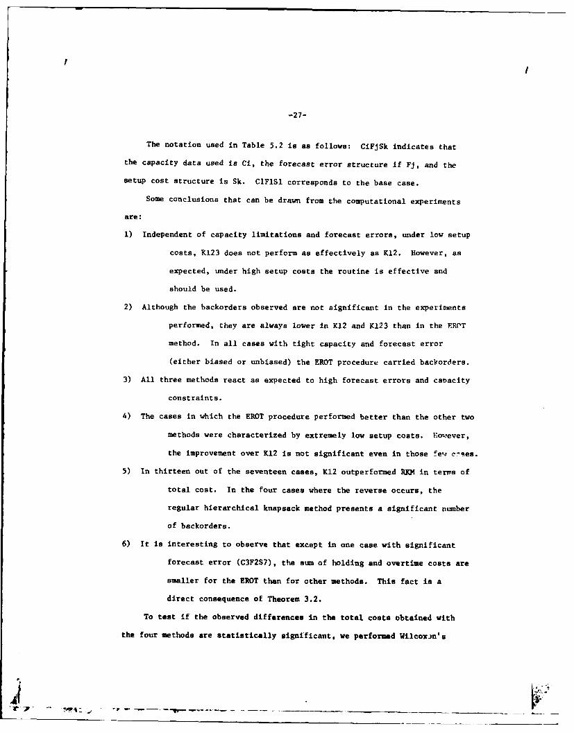
The notation used in Table 5.2 is as follows: CiFjSk indicates that
the capacity data used is Ci, the forecast error structure if Fj, and the
setup cost structure is Sk. CIFISi corresponds to the base case.
Some conclusions that can be drawn from the computational experiments
are:
1) Independent of capacity limitations and forecast errors, under low setup
costs, K123 does not perform as effectively as K12. However, as
expected, under high setup costs the routine is effective and
should be used.
2) Although the backorders observed are not significant in the experintents
performed, they are always lower in K12 and K123 than in the FROT
method. In all cases with tight capacity and forecast error
(either biased or unbiased) the EROT procedure carried backorders.
3) All three methods react as expected to high forecast errors and caDacity
constraints.
4) The cases in which the EROT procedure performed better than the other two
methods were characterized by extremely low setup costs. However,
the improvement over K12 is not significant even in those fe7q c-qes.
5) In thirteen out of the seventeen cases, K12 outperformed RKM in terms of
total cost. In the four cases where the reverse occurs, the
regular hierarchical knapsack method presents a significant number
of backorders.
6) It is interesting to observe that except in one case with significant
forecast error (C3F2S7), the sum of holding and overtime costs are
smaller for the EROT than for other methods. This fact is a
direct consequence of Theorem 3.2.
To test if the observed differences in the total costs obtained with
the four methods are statistically significant, we performed Wilcoxin's
L 7W:-~---~----- ______________ ____

-28-
Table 5.2: A Comparison of the Costs Resulting When the Various ApproachesWere Tested on Sample Points
CASE . COST TYPE RKM K12 K123 EROT BEST M.I.P.SOLUTION FOUND
Base Holding 29920 30651 45476 29923Case Setup 5580 5360 5030 5910
ClFlSl Overtime 81684 81113 72319 81681
Total 117184 117120 122825 117514 115616
Setup/Total 4.8% 4.6% 4.1% 5.0%Z Difference iin% ifrneit 1.4 1.3 6.2 1.6Cost from M.I.P.
Backorders - - - -
ClFlS8 Holding 31221 33195 30739 29923Setup 11910 12610 12210 13910Overtime 82382 79302 81682 81682
Total 125513 125107 124631 125515 122790
Setup/Total 9.5% 10.1% 9.q% 11.1%
% Difference inCost from M.I.P.
Backorders 71 units - - -
CIFIS5 Holding 31922 32028 35921 29923Setup 67050 67050 54650 68850Overtime 81682 80926 79714 81681
Total 180654 180004 170285 180454 165550
Setup/Total 37.1% 37.2% 32.1% 38.2%
% Difference inCost from M.I.P.
Backorders 4 units - - -
C2FlS5 Holding 13581 14042 47784 13584Setup 67850 67050 53850 68850Overtime 48577 48878 24681 47578
Total 130010 129970 126315 130012 124236
Setup/Total 52.2% 51.6% 42.6% 53.0%
% Difference in 4.9 4.6 1.7 4.6Cost from M.I.P.
Backorders - - - -
'Af -I

I | |
-29-
CASE COST TYPE RKM K12 K123 EROT
ClF2Sl Holding 64380 65473 65386 63806
Setup 4740 5070 5030 5730Overtime 80957 78907 78657 79709
Total 150077 149450 152073 149245
Setup/Total 3.2 3.4 3.3 3.8
Backorders 5 units - - -
ClF3S1 Holding 83034 86315 94553 78197Setup 4300 5180 5070 5910Overtime 88396 83491 80303 90412
Total 175730 174986 179926 174519
Setup/Total 2.5 3.0 2.8 3.4
Backorders - - - -
C1F3S7 Holding 85343 90295 89088 78197Setup 194000 171300 152200 203700Overtime 88753 77729 85709 90412
Total 368096 339324 326997 372309
Setup/Total 52.7 50.5 46.5 54.7
Backorders 6 units - - -
C2F1S1 Holding 13584 13584 21849 13584Setup 5910 5910 5310 5910Overtime 48878 47578 42237 47578
Total 68371 67072 68396 67072
Setup/Total 8.6 8.8 7.8 8.8
Backorders - - - -
C2F1S7 Holding 13583 14066 59739 13584Setup 200500 195300 134100 203700Overtime 48878 48878 28047 47578
Total 262961 258244 221881 264862
Setup/Total 76.2 75.6 60.4 74.0
Backorders - - -

-30-
CASE COST TYPE RKM K12 K123 EROT
C2F2S1 Holding 49856 49856 53721 49856Setup 5730 5730 5400 5910Overtime 50269 48523 47503 48523
Total 105855 104109 106624 104289
Setup/Total 5.4 5.5 5.1 5.7
Backorders - - - -
C3FlS1 Holding 73016 76157 82455 77584Setup 3930 4480 4480 5910Overtime 118560 117326 111320 112560
Total 195506 197963 198255 196054
Setup/Total 2.0 2.3 2.3 3.n
Backorders 5522 units - - -
C3F1S7 Holding 71584 92752 92678 77584Setup 198500 192700 172100 203700Overtime 118560 98960 99830 112560
Total 388645 384412 364608 393844
Setup/Total 51.1 50.1 47.2 51.7
Backorders 6942 units - - -
C3F2S1 Holding 84620 100304 106213 80986Setup 4300 4920 4810 5910Overtime 118560 92930 88600 108243
Total 207480 198154 199623 195139
Setup/Total 2.1 2.5 2.4 3.0
Backorders 8159 units 301 units 301 units 1412 units
C3F2S7 Holding 84842 97526 108409 82986Setup 202900 195300 178700 203700Overtime 118560 91634 91450 108243
Total 406302 384460 378559 392929
Setup/Total 49.9 50.8 47.2 51.8
Backorders 6178 units - - -
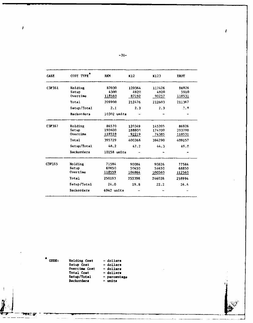
-31-
CASE COST TYPE RKM K12 K123 EROT
C3F3Sl Holding 87030 120364 117426 86926Setup 4300 4920 4920 5910Overtime 118560 87192 90257 118531
Total 209900 212476 212603 211367
Setup/Total 2.1 2.3 2.3 1.9
Backorders 10302 units - - -
C3F3S7 Holding 86570 120349 145205 86926Setup 190600 188800 174700 203700Overtime 118559 92219 74385 118531
Total 395729 400368 394290 409157
Setup/Total 48.2 47.2 44.3 49.S
Backorders 10158 units - - -
C3F1S5 Holding 71584 90084 90826 77584Setup 60050 50450 54650 68850Overtime 118559 104864 100560 112560
Total 250193 255398 246038 258994
Setup/Total 24.0 19.8 22.2 26.6
Backorders 6942 units - - -
CODE: Holding Cost - dollarsSetup Cost - dollarsOvertime Cost - dollarsTotal Cost - dollarsSetup/Total - percentageBackordera - units

-32-
signed rank test. The test was used to pairwise compare the methods. The
null hypothesis is that the total costs of the first approach are less than
or equal to those of the second. Table 5.3 shows the results obtained
for the Wilcoxon's test. WI is the Wilcoxon statistics and a is its standard
deviation.
Table 5.3: Results Obtained for the Wilcoxon's Test
Confidence withwhich null hypo-thesis can be
Methods Compared Wilcoxon Statistics Sample Size rejec ted
RKM vs. K12 WI = 1.81o 17 96,
RKM vs. K123 WI - 1.900 17 97"
K12 vs. K123 WI = 5.36a 72 >99%
EROT vs. K123 WI = 5.530 72 >99
The Wilcoxon statistics indicate that overall, the adjusted knipspc"- i Tith
feedback is superior to all other approaches. However, our detailed analysis
suggests that if the setup costs are very small, i.e., less than InT of th-
total cost, the feedback algorithm should not be used.
The second set of experiments consisted in solving a selected sample of
the seventy two problems as mixed integer programming problems (MIP). The
formulation of the production planning problems as MIP's can be seen as an
optimal representation. The four problems shown in Table 5.4 were solved
using the Land and Powell package on the computer Prime 400 at M.I.T.
Unfortunately, although each problem contains only sixty five zero-one
variables, no "true optimal" solution was found within forty hours of connect
time for each of the four problems. In Table 5.4 we indicate the best solu-
tion available at time of interruption of the computer programs. Due to the
poor performance of the mixed integer package we limited the experiments to
- . -I w- - -

I I
-33-
only four problems which were solved just once (rather than on a rolling
horizon basis). This last fact favors the MIP formulations. To facilitate
the comparison between the methods, the results corresponding to the four
problems obtained in Table 5.2 for the RKM, K12, K123, and EROT algorithms are
repeated in Table 5.4.
Table 5.4: Total Costs
ClFlSl ClFS5 ClFlS8 C2FS5
RKM 117184 180654 125513 130010
K12 117120 180004 125107 129970
K123 122825 170285 124631 126315
EROT 117514 180454 125515 130012Best MIPsti 115616 165550 122790 124236Soiut on
The results in Table 5.4 indicate that when the setup costs are less
than 5% of total costs and K12 is used, or when the setup costs are preater
than 5% and K123 is used, the total annual costs were never more than 3%
greater than the best MIP solution found after forty hours of connect time.
Finally we point out that none of the seventy two problems solved by the
RKM, K12, K123, and EROT algorithms on a rolling horizon basis, i.e.
solved thirteen times over the horizon of one year, exceeded ten minutes of
connect time on the M.I.T. computer Prime 400.
I
LL..o
-34-
6. CONCLUSIONS
The experimentation reported herein tends to confirm our belief that
hierarchical planning systems provide a very effective alternative for
supporting production planning decisions at a tactical and operational
level. When contrasted with a mixed integer programming formulation, hier-
archical planning methods produce near optimal solutions with significantly
smaller computational efforts and data collection requirements. The
hierarchical planning approach represents a feasible alternative for the
solution of large scale real life problems which will be unthinkable to
tackle with an M.I.P. based model. Moreover, and most important from a
pragmatic point of view, the hierarchical approach parallels the hierarchy of
production planning decisions within the firm.
From a methodological point of view, our experiments seem to indicate
that the modifications introduced to the Regular Knapsack Method clearly
improve the performance of previous algorithms. The K123 method, under the
wide variety of situations tested, outperforms statistically all other
methodological alternatives considered. However, a closer examination of
those cases where setup costs account for less than ten percent of the total
production cost indicates that K12 or EROT might be preferred over K123.
EROT and 1K12 tend to perform quite closely under low setup cost conditions.
ACKNOWLEDGEMENTS
The authors would like to express their gratitude to Josep Valor, for
his computational assistance, and Prof. Stephen C. Graves for many insightful
couents.
I !
-35-
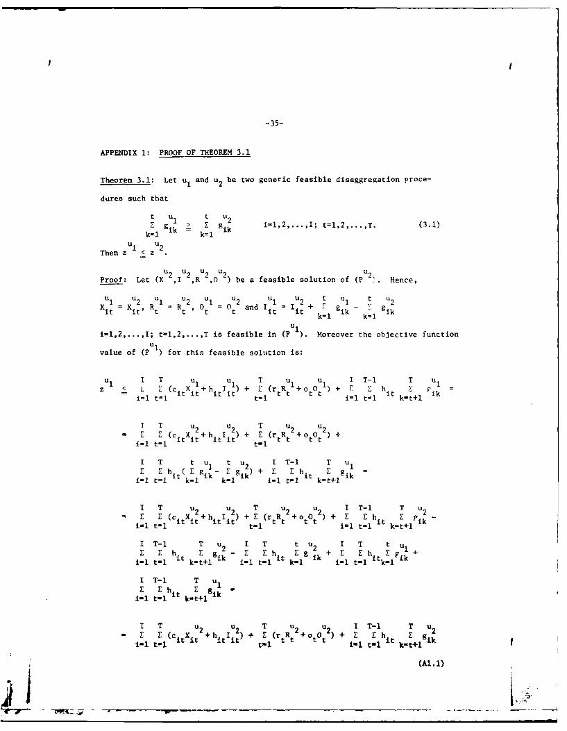
APPENDIX 1: PROOF OF THEOREM 3.1
Theorem 3.1: Let u and u2 be two generic feasible disaggregation proce-
dures such that
t uI t u2E g k Z gk i=1,2,....I; t=,2,...,T. (3.1)
k=l k=lu1 u2
Then z 1< z
u2 u 2u 2u u 2Proof: Let (X ,I ,R 2,0 ) be a feasible solution of (P . Hence,
uI u R u2 oU u u u2 t uI t u2u1 u2 u1 U2 u1 u2 u1 u2 t U1 t U 2
Xit =X Ri = R t = 0 t2 and it Iit + r _ gk=l k=l
i=1,2,...,I; t-1,2,...,T is feasible in (PU). Moreover the objective function
value of (P u l) for this feasible solution is:
u I T u u1 T u1 u1 I T-1 T u1z < E Z (ci.t X +hi I it + t (rtR t +oO t ) + E Z h.it Z p =
i=l t=l t=l i=l t=l k-t+l
I T u2 u 2 T u2 u 2
E E (cit Xt+h itit + Z (rtRt +oO t ) +i=l t=l t=l
I T t u1 t u2 I T-1 T uIEkl ik Egik)+ E E h i
i=l t kI i=l tl i k=t+l
I T u2 u2 T u2 u2 I T-1 T u2E(citXit +hitit ) + E (rtR t +ot0t ) + E E h iiki-l t=l t=l i.1 t=lh i k-t4-1
I T-1 T u2 I T t U2 I T t u
E E h it E g 2EEh it E 9 .k+ E E hitEp ik~i-1 t=l k=t+l i-l t=l k=1 i-i t1 k-l
I T-1 T u1
E Ehi iki-1 t-1 k-t+l
I T u2 u2 T u2 u2 I T-1 T u22 E (citXit +hitIit) + E (rtRt +otO t + Z hit gilt-l t.1 iftl t= h k- +I1

! I
-36-
T uI T u
The last inequality in (3.2) follows from the fact that E gk = 2
k- ik k=l k ii=1,2, ....I. The conclusion that can be drawn from (Al.I) is that the
optimal value of problem (P I) is not higher than the value of the objec-
tive function of problem (Pu 2) for any feasible solution in (Pu 2 ) that is,uI U2
z <z
Theorem 3.1 indicates that any two feasible disaggregation procedures
are not necessarily comparable in terms of total aggregate production costs.
It is important to note however that the optimal value zu of (PU) used to
compare disaggregation schemes is a proxy for the total production cost of
the hierarchical method.
I

-37-
APPENDIX 2: PROOF OF THEOREM 3.2
Theorem 3.2: Let uE denote the EROT disaggregation procedure. Then, if
all disaggregations are made with the EROT disaggregation method, if
I > 0 for all product types, and if the aggregate product type 3robler
(PO) is feasible it follows that' E
o t EZ Z
bProof: Every summation Y with b < a is defined as being zero. Lt uE
tzadenote the EROT disaggregation procedure and assume that all disaggrenations
are made using this method. Let I ? 0, i=l,2,...,l, be the init4 rn-
tory of product type i before the computations of the effective derani-.
Recall that safety stocks are not included in the I o for i=1,2,..., T .
Denote by dit the real demand of product type i in time period t for
i=l,2,...,I and t=l,2,...,T. Since the EROT disaggregation procedure is being
used each inventory Iio will last for R(i) periods where
r(i) _
I - E dit
R(i) = r(i) + t=l 1=1,2,..., I (P2.1)dir(i)+l
r(i) is the smallest nonnegative integer satisfying
r(i)+lI o - Z dit < 0
Moreover, the product type problem (P ) that we need to solve at the begin-u E
ning of period 1 is such that the git are nonnegative and satisfy for eachI UEi-I,2,...,T the condition I °ot I gtt The first term in (A2.1) is the
smallest integer less than or equal to R(i).
The EROT disaggregation method implies that for each product type
i1,2,...,I one of two following cases occur:
-i~-- ______ <-
-38-
a) If r(i) > 1 then g dit, t=1,2,... ,r(i), and (A2.2)
r(i) _UE0<u E <a
= io k=i ik = gir(i)+l ir(i)+l (P2.3)
b) If r(i) < 1 then I = gE < (A2.4)io ii i
Assume that (Po) is feasible and that (X , I,R ,O) is one of its optimal
solutions. Define
uE o E 0 t t t
X, RE = Ro , oE= Oo and IE = X - E d + E giE
itR k1l ik k1ik klik
t=l,2,...,T; i=1,2,...,I. (A2.5)
To show that (X E,I E,R ,LO ) is feasible in (pu E) we still need to proveuE
that it satisfies the mass balance constraints and that I > 0.
First we prove that the mass balance constraints hold at (X EIE, ,O U E).
uE uE uE t-i 0 t-l t-l uE o t 0 t uI _+ X itI E ~Xi - Edak+ E Zikx 1 - Xik + E d ik Eiit- It it k=lk k=l ik1 L i k1l i k=l -
- 2 1-1,2,...,I; t=l,2, .. ,T. (A2.6)it i1t
the first equality in (A2.6) follows from (A2.5).
Next, we prove that I > 0. Note that
uE to01) for 1< it < r(i), I = X 0, i>1,2,...,I by (A2.2)
ki
2) for t = r(i)+l
UE r(i)+l r(i)+l r(i)+l uElIr)+ E E o E + Eir(i)+l k1 ik k-I ik k.i ss
r(i)+l 0 r(i)+l - - 10r X E d ik
k.1 ik k- I io ir(i)+l - 0
the second equality follows from (A2.2), (A2.3), and (A2.4) since they

-39-
r(i)+l uimply that i = E gik;
k=l
3) for t > r(i)+l,
uE t 0 t t uE t t
-it Exik dik Xk - d + _-k=1 k=1 k.1 k=l k.1
= IO > 0. 1-1,2,..,1;it =
the second equality follows from (A2.2), (A2.3), and (A2.4) since t-pyr(i)+I uE UEimply that I o E R ik and hence gik 0O k=r()+2,...,T.k=1
uE uE uE uE uFrom 1), 2), and 3) we have that (X ,I ,R ,O ) is feasible in (P E).
Therefore,
UE I T UI Ui T UE u I T-I T. E (ctx Et+h IE) + r. (r R) + E F hi t=it it it it t t i=l t=1 i t k=
I T t t t= E [c Xit+htEiX - + E )] +
it it it ik ik ik1=1 t=l k=1 k1l k=1
T u E uE I T-I T u+ E (rtRt +ott0 ) + E E it g E -
t=l i=l t=l k=t+ k
I T t t TE E(c X + h (EX -Ed +1 )] + E (rR t +o tO t) +ik1 t k=1 t1
I T-I T u I T t u E+ E Eb h E E h1 (I E EgE)
1-1 t=l h i t k-t+l ik 1i t=1 hit llo k ik
I T TE E (ctX't+ h 1 0) + E (rR 0 +o 00) - zoi-i t-liti itt t-1 t t ) z
UE 0
hence, z < z.uE uE
However, from corollary 3.1, z0 < z . Consequently z = z E
--..a

-40-
References
1. Bitran, G. R.. E. Haas, and A. C. Hax, "Hierarchical Production Planning:A Multi Stage System", M.I.T., Operations Research Center, TechnicalReport No. , 1980.
2. Bitran, G. R., and A. C. Hax, "On the Design of Hierarchical ProductionPlanning Systems", Decision Sciences, Vol. 8, No. 1, January 1177,pp. 28-55.
3. Bitran, G. R., and A. C. Hax, "On the Solution of Convex KnapsackProblems with Bounded Variables", M.I.T., Operations Research Center,Technical Report No. 129, April 1977.
4. Bowman, E. H., "Production Scheduling by the Transportation Method ofLinear Programming", Operations Research, Vol. 4, No. 1, February 1956,pp. 100-103.
5. Bowman, E. H., "Consistency and Optimality in Managerial DecisionMaking", Management Science, Vol. 9, No. 2, January 1963, pp. 310-321.
6. Buffa, E. S., and J. G. Miller, Production-Inventory Systems: Planningand Control, Irwin, 1979.
7. Dzielinski, B. P., C. T. Baker, and A. S. Manne, "Simulation Tests ofLot Size Programming", Management Science, Vol. 9, No. 2, January 1963,pp. 229-258.
8. Dzielinski, B. P., and R. E. Gomory, "Optimal Programming of LotSizes, Inventory and Labor Allocations", Management Science, Vol. 11,No. 9, July 1965, 874-890.
9. Gabbay, H., "A Hierarchical Approach to Production Planning", M.I.T.,Operations Research Center, Technical Report No. 120, December 1975.
10. Golovin, J. J., "Hierarchical Integration of Planning and Control",M.I.T., Operations Research Center, Technical Report No. 116, September1975.
11. Hanssmann, F., and S. W. Hess, "A Linear Programing Approach toProduction and Employment Scheduling", Management TechnoloRy, No. 1,January 1960, pp. 46-51.
12. Hax, A. C., "Aggregate Production Planning", in Handbook of OperationsResearch, J. Moder and S. E. Elmaghraby (eds.), Van Nostrand Reinhold,1978.
13. Hax, A. C., "The Design of Large Scale Logistics Systems: A Surveyand an Approach", in Modern Trends in Logistics Research, W. F. Yarlow(ed.), MIT Press, 1976.
14. Hax, A. C., and J. J. Golovin, "Hierarchical Production PlanningSystems", in Studies in Operations Management, A. C. Hax (ed.), NorthHolland, 1978.

-41-
15. Hax, A. C., and H. C. Meal, "Hierarchical Integration of Production
Planning and Scheduling", in Studies in Management Sciences, Vol. I,Logistics, M. A. Geisler (ed.), North Holland-American Elsevier, 1975.
16. Holt, C. C., F. Modigliani, J. F. Muth, and H. A. Simon, Plannin"Production, Inventories and Work Force, Prentice Hall, 1960.
17. Johnson, L. A., and D. C. Montgomery, Operations Research in ProductionPlanning, Scheduling and Inventory Control, John Wiley, 1974.
18. Jones, C. H. "Parametric Production Planning", Management Science,Vol. 13, No. 11, July 1967, pp. 843-866.
19. Lasdon, L. S., and R. C. Terjung, "An Efficient Algorithm for Multi-Item Scheduling", Operations Research, Vol. 19, No. 4, 1971,pp. 946-969.
20. Manne, A. S., "Programming to Economic Lot Sizes", Management Science,Vol. 4, No. 2, 1958, pp. 115-135.
21. Newson, E. P., "Multi-Item Lot Size Scheduling by Heuristic, Part I:With Fixed Resources, Part II: With Variable Resources", ManagementScience, Vol. 21, No. 10, July 1975.
22. Peterson, R., and E. A. Silver, Decision Systems for Inventory Manage-ment and Production Planning, John Wiley, 1979.
23. Shwimer, J., "Interactions Between Aggregate and Detailed Schedulingin a Job Shop", unpublished Ph.D. Thesis, Alfred P. Sloan School ofManagement, M.I.T., June 1972.
24. Silver, E. A., and H. C. Meal, "A Heuristic for Selecting Lot Size
Quantities for the Case of a Deterministic Time Varying Demand Rateand Discrete Opportunities for Replenishment", Production and InventoryManagement, second quarter, 1973.
25. Taubert, W. H., "A Search Decision Rule for the Aggregate SchedulingPattern", Management Science, Vol. 14, No. 6, February 1968.
26. Wagner, H. M., and T. M. Whitin, "Dynamic Version of the Economic Lot
Size Model", Management Science, Vol. 5, No. 1
27. Winters, P. R., "Constrained Inventory Rules for Production Smoothing",Management Science, Vol. 8, No. 4, July 1962.
28. Zoller, K., "Optimal Disaggregation of Aggregate Production Plans",Management Science, Vol. 17, No. 8, April 1971, p;. B533-B547.
L