Any modification of the Born rule leads to a violationof the purification and local tomography principlesThomas D. Galley and Lluis Masanes

Department of Physics and Astronomy, University College London, Gower Street, London WC1E 6BT, United KingdomNovember 5, 2018

Using the existing classification of all al-ternatives to the measurement postulates ofquantum theory we study the properties ofbi-partite systems in these alternative the-ories. We prove that in all these theoriesthe purification principle is violated, mean-ing that some mixed states are not the reduc-tion of a pure state in a larger system. Thisallows us to derive the measurement postu-lates of quantum theory from the structure ofpure states and reversible dynamics, and therequirement that the purification principleholds. The violation of the purification prin-ciple implies that there is some irreducibleclassicality in these theories, which appearslike an important clue for the problem of de-riving the Born rule within the many-worldsinterpretation. We also prove that in all suchmodifications the task of state tomographywith local measurements is impossible, andpresent a simple toy theory displaying allthese exotic non-quantum phenomena. Thistoy model shows that, contrarily to previousclaims, it is possible to modify the Born rulewithout violating the no-signalling principle.Finally, we argue that the quantum measure-ment postulates are the most non-classicalamongst all alternatives.

1 IntroductionThe postulates of quantum theory describe the evo-lution of physical systems by distinguishing betweenthe cases where observation happens or not. How-ever, these postulates do not specify what consti-tutes observation, and it seems that an act of obser-vation by one agent can be described as unperturbeddynamics by another [1]. This opens the possibilityof deriving the physics of observation within the pic-ture of an agent-free universe that evolves unitarily.

Thomas D. Galley: thomas.galley.14@ucl.ac.uk

This problem has been studied within the dynam-ical description of quantum measurements [2], thedecoherence program [3] and the Many-Worlds In-terpretation of quantum theory [4, 5].

In this work, instead of presenting another deriva-tion of the measurement postulates, we take a moreneutral approach and analyze all consistent alter-natives to the measurement postulates. In particu-lar, we prove that in each such alternative there aremixed states which are not the reduction of a purestate on a larger system. This property singles outthe (standard) quantum measurement postulates in-cluding the Born Rule.

In our previous work [6] we constructed a com-plete classification of all alternative measurementpostulates, by establishing a correspondence be-tween these and certain representations of the uni-tary group. However, this classification did not in-volve the consistency constraints that arise from thecompositional structure of the theory; which governshow systems combine to form multi-partite systems.In this work we take into account compositionalstructure, and prove that all alternative measure-ment postulates violate two compositional princi-ples: purification [7, 8] and local tomography [9, 10].We also present a simple alternative measurementpostulate (a toy theory) which illustrates these ex-otic phenomena. Additionally, this toy theory pro-vides an interesting response to the claims that theBorn rule is the only probability assignment consis-tent with no-signalling [11–13].

In Section 2 we introduce a theory-independentformalism, which allows to study all alternatives tothe measurement postulates. We also review theresults of our previous work [6]. In Section 3 wedefine the purification and local tomography princi-ples, and show that these are violated by all alter-native measurement postulates. In Section 4 we de-scribe a particular and very simple alternative mea-surement postulate, which illustrates our general re-sults. In Section 5 we discuss our results in the light

1

arX

iv:1

801.

0641

4v4

[qu

ant-

ph]

1 N

ov 2

018

of existing work. All proofs are in the appendices.

2 Dynamically-quantum theoriesIn this work we consider all theories that have thesame pure states, dynamics and system-compositionrule as quantum theory, but have a different struc-ture of measurements and a different rule for assign-ing probabilities.

2.1 States, transformations and composition pos-tulatesThe family of theories under consideration satisfythe following postulates, taken from the standardformulation of quantum theory.

Postulate (Quantum States). Every finite-dimensional Hilbert space Cd corresponds to a typeof system with pure states being the rays ψ of Cd.

Postulate (Quantum Transformations). The re-versible transformations on the pure states Cd areψ 7→ Uψ for all U ∈ SU(d).

Postulate (Quantum Composition). The joint purestates of systems CdA and CdB are the rays of CdA ⊗CdB ' CdAdB .

2.2 Measurement postulatesBefore presenting the generalized measurement pos-tulate we need to introduce the notion of outcomeprobability function, or OPF. For each measurementoutcome x of system Cd there is a function F (x)

that assigns to each ray ψ in Cd the probabilityF (x)(ψ) ∈ [0, 1] for the occurrence of outcome x.Any such function F is called an OPF. Each systemhas a (trivial) measurement with only one outcome,which must have probability one for all states. Theuniqueness of this trivial measurement is the Causal-ity Axiom of [7]. The OPF associated to this out-come is called the unit OPF u, satisfying u(ψ) = 1for all ψ. A k-outcome measurement is a list of kOPFs (F (1), . . . , F (k)) satisfying the normalizationcondition

∑i F

(i) = u. It is not necessarily the casethat every list of OPFs satisfying this condition de-fines a measurement, though this assumption can bemade. As an example, the OPFs of quantum theoryare the functions

F (ψ) = tr(F |ψ〉〈ψ|) , (1)

for all Hermitian matrices F satisfying 0 ≤ F ≤ I.This implies that u = I. (Here and in the rest ofthe paper we assume that kets |ψ〉 are normalized.)

Postulate (Alternative Measurements). Everytype of system Cd has a set of OPFs Fd with a bi-linear associative product ? : FdA × FdB → FdAdBsatisfying the following consistency constraints:

C1. For every F ∈ Fd and U ∈ SU(d) there isan F ′ ∈ Fd such that F ′(ψ) = F (Uψ) for allψ ∈ Cd. That is, the composition of a unitaryand a measurement can be globally considereda measurement.

C2. For any pair of different rays ψ 6= φ in Cd thereis an F ∈ Fd such that F (ψ) 6= F (φ). Thatis, different pure states must be operationallydistinguishable.

C3. The ?-product satisfies uA ? uB = uAB and

(FA ? FB)(ψA ⊗ φB) = FA(ψA)FB(φB) , (2)

for all FA ∈ FdA , FB ∈ FdB , ψA ∈ CdA , φB ∈CdB . That is, tensor-product states ψA ⊗ φBcontain no correlations.

C4. For each φAB ∈ CdA ⊗ CdB and FB ∈ FdB thereis an ensemble {(ψiA, pi)}i in CdA such that

(FA ? FB)(φAB)(uA ? FB)(φAB) =

∑i

piFA(ψiA) , (3)

for all FA ∈ FdA . That is, the reduced stateon A conditioned on outcome FB on B (and re-normalized) is a valid mixed state of A. In thenext sub-section we fully articulate the notionsof ensemble and mixed state.

C5. Consider measurements on system CdA with thehelp of an ancilla CdB . For any ancillary stateφB ∈ CdB and any OPF in the composite FAB ∈FdAdB there exists an OPF on the system F ′A ∈FdA such that

F ′A(ψA) = FAB(ψA ⊗ φB) (4)

for all ψA.

The derivation of these consistency constraints fromoperational principles is provided in Appendix A.Continuing with the example of quantum theory (1),the ?-product in this case is

(FA ? FB)(ψAB) = tr(FA ⊗ FB|ψAB〉〈ψAB|) . (5)

A trivial modification of the Measurement Postulateconsists of taking that of quantum mechanics (1)and restricting the set of OPFs in some way, suchthat not all POVM elements F are allowed. In thiswork, when we refer to “all alternative measurementpostulates” we do not include these trivial modifi-cations.

2

2.3 Mixed states and the Finiteness PrincipleA source of systems that prepares state ψi ∈Cd with probability pi is said to prepare the en-semble {(ψi, pi)}i. Two ensembles {(ψi, pi)}i and{(φj , qj)}j are equivalent if they are indistinguish-able ∑

i

piF (ψi) =∑j

qjF (φj) (6)

for all measurements F ∈ Fd. Note that distin-guishability is relative to the postulated set of OPFsFd. A mixed state ω is an equivalence class of indis-tinguishable ensembles, and hence, the structure ofmixed states is also relative to Fd. To evaluate anOPF F on a mixed state ω we can take any ensemble{(ψi, pi)}i of the equivalence class ω and compute

F (ω) =∑i

piF (ψi) . (7)

In general, ensembles can have infinitely-manyterms, hence, the number of parameters that areneeded to characterize a mixed state can be infinitetoo. When this is the case, state estimation withoutadditional assumptions is impossible, and for thisreason we make the following assumption.

Principle (Finiteness). Each mixed state of afinite-dimensional system (Cd,Fd) can be character-ized by a finite number Kd of parameters.

Recall that in quantum theory we have Kd = d2 −1. And in general, the distinguishability of all raysin Cd implies Kd ≥ 2d − 2. These Kd parameterscan be chosen to be a fix set of “fiducial” OPFsF1, . . . , FKd

∈ Fd, which can be used to representany mixed state ω as

ω =

F1(ω)F2(ω)

...FKd

(ω)

. (8)

The fact that OPFs are probabilities implies thatany OPF F ∈ Fd is a linear function of the fiducialOPFs

F =∑i

ciFi . (9)

In other words, the fiducial OPFs F1, . . . , FKd∈ Fd

constitute a basis of the real vector space spanned byFd. Using the consistency constraint C1, we definethe SU(d) action

Fi =∑i′

Γi,i′(U)Fi′ (10)

on the vector space spanned by Fd. This asso-ciates to system (Cd,Fd) a Kd-dimensional repre-sentation of the group SU(d). This, together withthe other consistency constraints, implies that onlycertain values of Kd are allowed. For exampleK2 = 3, 7, 8, 10, 11, 12, 14 . . .

2.4 Measurement postulates for single systemsIn this subsection we review some of the results ob-tained in [6]. These provide the complete classifica-tion of all sets Fd satisfying the Finiteness Principleand the consistency constraints C1 and C2. Theseresults ignore the existence of the ?-product, C3, C4and C5. Hence, in alternative measurement postu-lates with a consistent compositional structure therewill be additional restrictions on the valid sets Fd.This is studied in Section 3.

Theorem (Characterization). If Fd satisfies theFiniteness Principle and C1 then there is a posi-tive integer n and a map F 7→ F from Fd to the setof dn × dn Hermitian matrices such that

F (ψ) = tr(F |ψ〉〈ψ|⊗n

)(11)

for all normalized vectors ψ ∈ Cd.Note that there are many different sets Fd with thesame n. In particular, since the SU(d) action

|ψ〉〈ψ|⊗n 7→ U⊗n|ψ〉〈ψ|⊗nU⊗n† (12)

is reducible, the Hermitian matrices F can have sup-port on the different irreducible sub-representationsof (12), generating sets Fd with very different phys-ical properties. All these possibilities are analyzedin [6].

Theorem (Faithfulness). If Fd satisfies the Finite-ness Principle, C1 and C2, thencase d ≥ 3 there is a non-constant F ∈ Fd.case d = 2 there is F ∈ F2 such that F has support

on a sub-representation of the SU(2) action (12)with odd angular momentum.

3 Features of all alternative measure-ment postulatesIn this section we analyze the compositional struc-ture of alternative measurement postulates. We doso by considering two well known physical principleswhich, together with other assumptions, have beenused to reconstruct the full formalism of quantumtheory [8, 14–16]. Remarkably, these principles areviolated by all alternative measurement postulates.

3

3.1 The Purification Principle

This principle establishes that any mixed state isthe reduction of a pure state in a larger system.This legitimises the “Church of the Larger HilbertSpace”, an approach to physics that always assumesa global pure state when an environment is addedto the systems under consideration [17].

Principle (Purification). For each ensemble{(ψi, pi)}i in CdA there exists a pure state φAB inCdA ⊗ CdB for some dB satisfying

(FA ? uB)(φAB) =∑i

piFA(ψi) , (13)

for all FA ∈ FdA .

Note that the original version of the purificationprinciple introduced in [7] additionally demandsthat the purification state φAB is unique up to aunitary transformation on CdB . Also note that thefollowing theorem does not require the FinitenessPrinciple.

Theorem (No Purification). All alternative mea-surements postulates Fd satisfying C1, C2, C3 andC4 violate the purification principle.

This implies that in all alternative measurementpostulates there are operational processes, such asmixing two states, which cannot be understood asa reversible transformation on a larger system. Insuch alternative theories, agents that perform physi-cal operations cannot be integrated in an agent-freeuniverse, as can be done in quantum theory, andthe Church of the Larger Hilbert Space is illegiti-mate. The assumption that agents’ actions can beunderstood as reversible transformations on a largersystem is also the starting point of the many-worldsinterpretation of quantum theory. Hence, it seemslike the no-purification theorem provides importantclues for the derivation of the Born Rule within themany-worlds interpretation [1, 3–5]. In section 5.1we discuss further the possibility of using this resultto derive the quantum measurement postulates, andcontrast it to Zurek’s envariance based derivation ofthe Born rule.

3.2 The Local Tomography Principle

This principle has been widely used in reconstruc-tions of quantum theory and the formulation of al-ternative toy theories [8, 14–16, 18, 19]. One of thereasons is that it endows the set of mixed states

with a tensor-product structure [10]. This princi-ple states that any bi-partite state is characterizedby the correlations between local measurements.That is, two different mixed states ωAB 6= ω′AB onCdA ⊗CdB must provide different outcome probabil-ities

(FA ? FB)(ωAB) 6= (FA ? FB)(ω′AB) (14)for some local measurements FA ∈ FdA , FB ∈ FdB .Using the notation introduced in (9) we can formu-late this principle as follows.

Principle (Local Tomography). If {Fa}a is a basisof FdA and {Fb}b is a basis of FdB then {Fa ? Fb}a,bis a basis of FdAdB , where a = 1, . . . ,KdA and b =1, . . . ,KdB .

A theory is said to violate local tomography if atleast one composite system within the theory vio-lates local tomography. Therefore, it is sufficient toanalyze the particular bi-partite system C3 ⊗ C3 =C9.

Theorem (No Local Tomography). All alternativemeasurements F3 and F9 satisfying C1, C2, C3 andthe Finiteness Principle violate the local tomogra-phy principle.

The above result is proven in Appendix E. We firstshow that all transitive theories which obey the localtomography principle have a group action acting onthe mixed states which has a certain structure. Anygroup action of the form (10) which does not havethis structure must correspond to a system which vi-olates local tomography. We show that all represen-tations of SU(9) which correspond to systems withalternative measurement postulates do not have thisstructure. This entails that all non-quantum C9 sys-tems which are composites of two C3 systems violatelocal tomography.

The technical result proven to show this is thefollowing. All non-quantum irreducible representa-tions of SU(9) which are sub-representations of theaction (12) have a sub-representation 13 ⊗ 13 whenrestricted to the subgroup SU(3) × SU(3). Here 13

denotes the trivial representation of SU(3).

3.2.1 Comment on C2 ⊗ C2 systems

In quantum theory any Cd (d ≥ 2) system can besimulated using some number of qubits. In thissense qubits can be viewed as fundemental informa-tion units [18]. Since C2 systems have a privelegedstatus it is natural to ask whether C4 = C2⊗C2 sys-tems in theories with modified measurement postu-lates are locally tomographic. The proof technique

4

used for the No Local Tomography Theorem appliesonly to a certain family of these C4 systems. How-ever all instances of C4 systems studied by the au-thors which were not part of this family were foundto not be locally tomographic. We conjecture thatall C4 = C2⊗C2 violate the local tomography prin-ciple.

4 A Toy TheoryIn this section we present a simple alternative mea-surement postulate (Fd, ?) which serves as exam-ple for the results that we have proven in general(violation of the purification and local tomographyPrinciples). In Appendix G it is proven that this al-ternative measurement postulate satisfies all consis-tency constraints (C1, C2, C3, C4, C5) except forthe associativity of the ?-product. This implies thatthis toy theory is only fully consistent when dealingwith single and bi-partite systems. However, mostof the work in the field of general probabilistic the-ories (GPTs) focuses on bi-partite systems, becausethese already display very rich phenomenology. Inthe following we consider two local subsystems of di-mension dA and dB with sets of OPFs FL

dAand FL

dB.

The composite (global) system has a set of OPFsFGdAdB

.

Definition (Local effects FLd ). Let S be the pro-

jector onto the symmetric subspace of Cd ⊗ Cd. Toeach d2 × d2 Hermitian matrix F satisfying

• 0 ≤ F ≤ S,

• F =∑i αi|φi〉〈φi|⊗2 for some |φi〉 ∈ Cd and

αi > 0,

• S− F =∑i βi|ϕi〉〈ϕi|⊗2 for some |ϕi〉 ∈ Cd and

βi > 0,

there corresponds the OPF

F (ψ) = tr(F |ψ〉〈ψ|⊗2

), (15)

The unit OPF corresponds to u = S.

That is, both matrices, F and S−F , have to be not-necessarily-normalized mixtures of symmetric prod-uct states.

Example (Canonical measurement for d prime).For the case where d is prime there exists a canon-ical measurement which can be constructed as fol-lows. Consider the (d+ 1) mutually unbiased bases(MUBs): {|φji 〉}di=1 where j runs from 1 to d+1 [20].

Then we can associate an OPF to each Hermitianmatrix 1

2 |φji 〉〈φ

ji |⊗2. Since the basis elements of these

MUBs form a complex projective 2-design [21], bythe definition of 2-design [22], we have the normal-ization constraint:

12∑i,j

|φji 〉〈φji |⊗2 = S , (16)

and hence the set of OPFs forms a measurement.

Definition (? product). For any pair of OPFs FA ∈FLdA

and FB ∈ FLdB

the Hermitian matrix correspond-ing to their product FA ? FB ∈ FG

dAdBis

FA ? FB = FA ⊗ FB + trFAtrSA

AA ⊗trFBtrSB

AB , (17)

where SA and AA are the projectors onto the sym-metric and anti-symmetric subspaces of CdA ⊗ CdA ,and analogously for SB and AB.

This product is clearly bilinear and, by using theidentity SAB = SA ⊗ SB + AA ⊗ AB, we can checkthat uA ? uA = uAB.

We observe that not all effects FA ? FB are of theform

∑i αi|φi〉〈φi|⊗2

AB. Hence the set of effects on thejoint system is not FL

dAdB, but has to be extended to

FGdAdB

to include these joint product effects.

Definition (Global effects FGdAdB

). The set FGdAdB

should include all product OPFs FA ? FB, all OPFsFLdAdB

of CdAdB understood as a single system, andtheir convex combinations.

The identity SAB = SA ⊗ SB +AA ⊗AB perfectlyshows that the vector space FG

dAdBis larger than the

tensor product of the vector spaces FLdA

and FLdB

, bythe extra term AA ⊗AB. This implies that this toytheory violates the Local-Tomography Principle.

The joint probability of outcomes FA and FB onthe entangled state ψAB ∈ CdA ⊗CdB can be writtenas

(FA ? FB)(ψAB)

=tr[(FA ⊗ FB + trFA

trSAAA ⊗ trFB

trSBAB)|ψAB〉〈ψAB|⊗2

].

When we only consider sub-system A outcome prob-abilities are given by

(FA ? uB)(ψAB)

= tr[(FA ⊗ SB + trFA

trSAAA ⊗AB

)|ψAB〉〈ψAB|⊗2

](18)

= trA

[FA ωA

], (19)

5

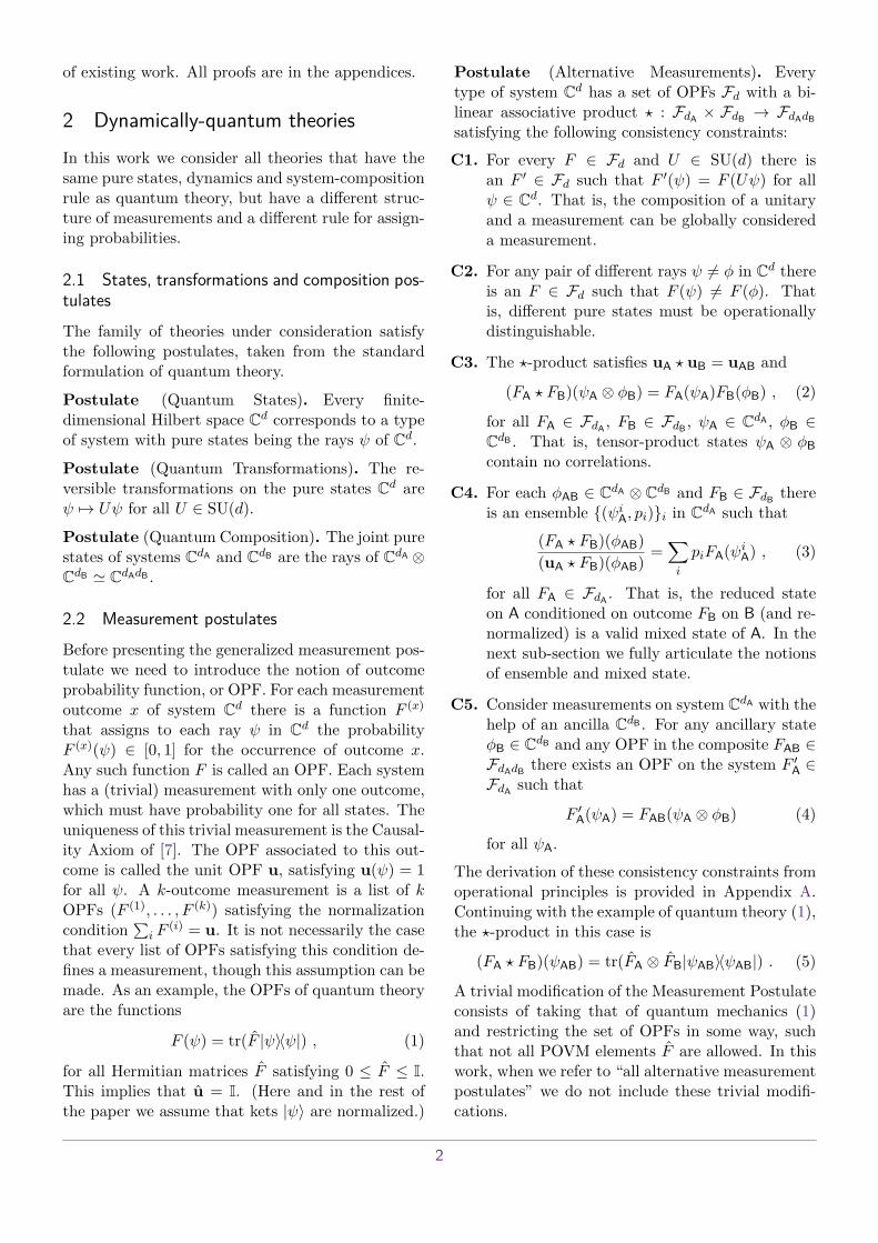
Figure 1: Projection of C2 toy model state space. In thisprojection the coloured points (blue and purple) are statesof the form

∑i pi|ψi〉〈ψi|⊗2. The blue points are projections

of reduced states of a larger system obtained using formula(20). The left hand corner corresponds to the state |0〉〈0|⊗2

and the right hand corner to the state |1〉〈1|⊗2. All purestates are projected onto the curved boundary. This figureshows that there are local mixed states (in purple) whichare not reduced states (in blue).

where the reduced state must necessarily be

ωA = trB(SB|ψAB〉〈ψAB|⊗2)+ SA

trSAtr(AAAB|ψAB〉〈ψAB|⊗2)

(20)All these reductions ωA of pure bipartite states ψABare contained in the convex hull of |φA〉〈φA|⊗2, as re-quired by the consistency constraint C4. However,not all mixtures of |φA〉〈φA|⊗2 can be written as onesuch reduction (20). That is, the purification pos-tulate is violated. This phenomenon is graphicallyshown in Figure 1.

This toy model violates the no-restriction hypoth-esis [7], in that not all mathematically allowed ef-fects on the local state spaces are allowed effects. Italso violates the principle of pure sharpness [23] inthat all the effects are noisy.

5 Discussion

5.1 Interpreting results as a derivation of the Bornrule

In this paper we have shown that all modifications tothe quantum measurements lead to violations of thepurification and local tomography principles. Thisentails that one can derive the measurement postu-lates of quantum theory from the structure of purestates and dynamics and either the assumption oflocal tomography or purification. Such a derivationuses the operational framework which can be viewedas a background assumption.

A derivation of the Born rule which starts fromsimilar assumptions to ours, but not within an op-erational setting, is the envariance based derivationof Zurek [3]. Zurek begins by assuming the dynami-cal structure of quantum theory and the assumptionthat quantum theory is universal, which is to say

that all the phenomena we observe can be explainedin terms of quantum systems interacting. Specifi-cally the classical worlds of devices can be modelledquantum mechanically, including the measurementprocess. We observe that this is philosophically verydifferent to the operational approach adopted in thiswork, which takes the classical world as a primitive.By assuming the dynamical structure of quantumtheory and the assumption of universality (as well assome auxiliary assumptions) Zurek shows that mea-surements are associated to orthonormal bases, andthat outcome probabilities are given by the Bornrule. For criticisms of Zurek’s approach we refer thereader to [24–27].

We observe that the purification postulate seemslinked to the notion that quantum theory is univer-sal, in the sense that any classical uncertainty canbe explained as originating from some pure globalquantum state. This shows an interesting link toZurek’s derivation, since although we work within anoperational framework, the concept of purificationis linked to the idea that quantum theory is univer-sal. This shows that we can also rely on a conceptlinked to universality in order to derive the Bornrule (and the structure of measurements) within anoperational approach.

We observe that we can also derive the measure-ment postulates of quantum theory from the as-sumption of local tomography, which does not havethis connotation of universality.

5.2 No-signallingMultiple proofs have been put forward which claimto show that violations of the Born rule lead to sig-nalling [11–13]. However the authors only considermodifications of the Born rule of a specific type. In[11, 12] the authors only consider modifications ofthe Born rule of the following form:

p(k|ψ) = |〈k|ψ〉|n∑k′ |〈k′|ψ〉|n

, (21)

where |ψ〉 =∑k αk |k〉. Modifications of this form

are very restricted. By modifying all the measure-ment postulates of quantum theory, we can cre-ate toy models like the one introduced, which arenon-signalling (as we will show momentarily). Thisshows that by modifying the Born rule in a moregeneral manner one can avoid issues of signalling.

In the case of the toy model it is immediate tosee that it is consistent with no-signalling. The con-dition of no-signalling is equivalent to the existenceof a well defined state-space for the subsystem (i.e.

6

independent of action on the other subsystem). Wesee then that no-signalling is just a consequence ofthere existing a well defined reduced state [7].

5.3 Purification as a constraint on physical theo-ries

In Theorem 19 of [7] the authors show that anytwo convex theories with the same states (pure andmixed) which obey purification are the same the-ory. In other words “states specify the theory” fortheories with purification [7]. In this chapter weshow that in the case of theories with pure statesPCd and dynamical group SU(d), any two theorieswhich obey purification with the same pure statesand reversible dynamics are the same. This meansthat for a restricted family of theories (those withsystems with pure states PCd and dynamical groupSU(d)) we have the same result as Theorem 19 of [7]but with different assumptions. It would be inter-esting to establish whether this is a general featureof theories with purification, namely that the purestates and reversible dynamics specify the theory.

5.4 The quantum measurement postulates arethe most non-classical

One consequence of the classification in [6] is thatthe quantum measurement postulates are the oneswhich give the lowest dimensional state spaces. Inthis sense the quantum measurement postulates arethe most non-classical, since they give rise to thestate spaces with the higest degree of indistinguish-able ensemles [28]. We remember that in classicalprobability theory all ensembles are distinguishable.

The violation of purification seems to indicatesome other, distinct type of classicality. In theorieswhich violate purification there are some prepara-tions which can only be modelled as arising from aclassical mixture of pure states. There appears to besome sort of irreducible classicality. However in the-ories which obey purification we can always modelsuch preparations as arising from the reduction of aglobal pure state. Since the quantum measurementpostulates are the only ones which give rise to sys-tems which obey purification they can be viewed asthe most non-classical amongst all alternatives.

Hence we see that according to these two distinctnotions of non-classicality the quantum measure-ment postulates are the most non-classical amonstall possible measurement postulates.

5.5 Toy modelThe toy model can be obtained by restricting thestates and measurements of two pairs of quantumsystems (CdA)⊗2 and (CdB)⊗2. In this sense we ob-tain a theory which violates both local tomographyand purification. This method of constructing the-ories is similar to real vector space quantum theory,which can also be obtained from a suitable restric-tion of quantum states and also violates local to-mography. The main limitation of the toy model isthat it does not straightforwardly extend to morethan two systems. There is a natural generalisationof the toy model to consider effects to be linear in|ψ〉〈ψ|⊗n for n > 2, however showing the consistencyof the reduced state spaces and joint effects is morecomplex.

5.6 Theories which decohere to quantum theoryA recent result [29] shows that all operational theo-ries which decohere to quantum theory (in an anal-ogous way to which quantum theory decoheres toclassical theory) must violate either purification orcausality (or both). The authors define a hyper-decoherence map which maps states of the post-quantum system to states of a quantum system (em-bedded within the post-quantum system). This mapobeys the following properties:

1. Terminality: applying the map followed by theunit effect is equivalent to just applying the uniteffect.

2. Idempotency: applying the map twice is thesame as applying it once.

3. The pure states of the quantum subsystem arepure states of the post-quantum system. Simi-larly the maximally mixed state of the quantumsubsystem is the maximally mixed state of thepost-quantum system.

Now we ask whether the systems in this paper(which violate purification) can correspond to post-quantum systems which decohere to quantum sys-tems in some reasonable manner. We consider thetoy model with pure states |ψ〉〈ψ|⊗2 and no restric-tion on the allowed effects (this toy model is onlyvalid for single systems). Now consider a linear mapfrom |ψ〉〈ψ|⊗2 to some embedded quantum systemsuch that the pure states of the system are also ofthe form |φ〉〈φ|⊗2 (by property 3). This map mustbe of the form U⊗2|ψ〉〈ψ|⊗2U †⊗2. Hence its actionon the state space conv

(|φ〉〈φ|⊗2) gives an identical

7

state space and the map is trivial.1 This shows thatthe only hyper-decoherence maps which obey all theconditions set out by Lee and Selby must be trivial.

As we argue later, it is not immediately obviousthat a hyper-decoherence map should obey condi-tion 3. We now define a hyper-decoherence like mapwhich does not meet this condition. Consider thefollowing map where we label the copies of |ψ〉〈ψ|, 1and 2:

D(|ψ〉〈ψ|⊗2) = Tr2(|ψ〉〈ψ|⊗2)⊗ |0〉〈0| (22)= |ψ〉〈ψ| ⊗ |0〉〈0| . (23)

This meets properties 1 and 2, but not 3. Indeedthe states |ψ〉〈ψ|⊗|0〉〈0| are not valid mixed states ofthe post-quantum system. The image of this map|ψ〉〈ψ| ⊗ |0〉〈0| for all ψ ∈ PCd is a quantum statespace.

The authors of [29] show that requirement 3 canbe replaced by the requirement that the hyper-decoherence map maps between systems with thesame information dimension. As shown in [6] (forthe case PC2) the information dimension of an un-restricted |ψ〉〈ψ|⊗2 state space is larger than that ofa qubit.

The hyper-decoherence map of [29] is inspired bythe decoherence map which exists between quantumand classical state spaces. The map introduced inthis section is very different from this, since its im-age is not an embedded state space; however it maybe that decoherence between a post-quantum the-ory and quantum theory is very different from whatour quantum/classical intuitions might lead us tobelieve.

The decoherence map of equation (22) appearsstrange at first, since it maps states of a post-quantum system to a sub-system which is embed-ded in such a way that its states are not valid statesof the post-quantum system. However the image ofthis decoherence map is actually the state space onewould obtain if one had access to the post-quantumsystem |ψ〉〈ψ|⊗2 but only a restricted set of mea-surements. An observer with access to the post-quantum system |ψ〉〈ψ|⊗2 but only effects of theform F (ψ) = Tr((F ⊗ I)|ψ〉〈ψ|⊗2) would reconstructa quantum state space. Hence the link between thesystem and subsystem becomes clearer: the quan-tum sub-system is obtained from the post-quantumsystem by restricting the measurements on the post-quantum system. We emphasise once more that thetoy model with unrestricted effects does not com-pose.

1We thank referee 1 for this observation.

6 Conclusion6.1 SummaryWe have studied composition in general theorieswhich have the same dynamical and compositionalpostulates as quantum theory but which have dif-ferent measurement postulates. We presented a toymodel of a bi-partite system with alternative mea-surement rules, showing that composition is possiblein such theories. We showed that all such theoriesviolate two compositional principles: local tomogra-phy and purification.

6.2 Future workThe toy model introduced in this work applies onlyto bi-partite systems and is simulable with quantumtheory. Hence an important next step is construct-ing a toy model with alternative measurement ruleswhich is consistent with composition of more thantwo systems. This requires a ? product which is as-sociative. This construction may prove impossible,or it may be the case that all valid constructionsare simulable by quantum theory. We suggest thatthere are three possibilities when considering theo-ries with fully associative products.

Possibility 1. (Logical consistency of postulates ofQuantum Theory). The only measurement postu-lates which are fully consistent with the associativ-ity of composition are the quantum measurementpostulates.

If this were the case it would show that the postu-lates of quantum theory are not independent. Onlythe quantum measurement rules would be consistentwith the dynamical and compositional postulates(and operationalism). However it may be the casethat we can develop theories with alternative Bornrules which compose with an associative product,but that all these theories are simulable by quan-tum theory.

Possibility 2. (Simulability of systems in theorieswith alternative postulates). The only measurementpostulates which are fully consistent with the dy-namical postulates of quantum theory describe sys-tems which are simulable with a finite number ofquantum systems.

Possibility 3. (Non-simulability of systems in theo-ries with alternative postulates). There exist mea-surement postulates which are fully consistent with

8

the dynamical postulates of quantum theory whichdescribe systems which are not simulable with a fi-nite number of quantum systems.

This final possibility would be interesting from theperspective of GPTs as it would show that there arefull theories which can be obtained by modifyingthe measurement postulates of quantum theory. Itwould show that quantum theory is not, in fact, anisland in theory space.

7 AcknowledgementsWe are grateful to Jonathan Barrett and RobinLorenz for helpful discussions. We thank the refereesfor their comments which helped substantially im-prove the first version of this manuscript. TG is sup-ported by the Engineering and Physical Sciences Re-search Council [grant number EP/L015242/1]. LMis funded by EPSRC.

References

[1] Hugh Everett. “Relative State” formulationof quantum mechanics. Rev. Mod. Phys., 29:454–462, Jul 1957. DOI: 10.1103/RevMod-Phys.29.454.

[2] A. E. Allahverdyan, R. Balian, and T. M.Nieuwenhuizen. Understanding quantum mea-surement from the solution of dynamical mod-els. Phys. Rep., 525:1–166, April 2013. DOI:10.1016/j.physrep.2012.11.001.

[3] Wojciech Hubert Zurek. Probabilities from en-tanglement, Born’s rule pk = | ψk |2 from en-variance. Phys. Rev. A, 71:052105, May 2005.DOI: 10.1103/PhysRevA.71.052105.

[4] David Deutsch. Quantum theory of probabilityand decisions. Proceedings of the Royal Societyof London A: Mathematical, Physical and En-gineering Sciences, 455(1988):3129–3137, 1999.DOI: 10.1098/rspa.1999.0443.

[5] David Wallace. How to Prove the Born Rule. InAdrian Kent Simon Saunders, Jon Barrett andDavid Wallace, editors, Many Worlds? Everett,Quantum Theory, and Reality. Oxford Univer-sity Press, 2010.

[6] Thomas D. Galley and Lluis Masanes. Classi-fication of all alternatives to the born rule interms of informational properties. Quantum, 1:15, jul 2017. DOI: 10.22331/q-2017-07-14-15.

[7] Giulio Chiribella, Giacomo Mauro DAriano,and Paolo Perinotti. Probabilistic theories withpurification. Physical Review A, 81(6):062348,jun 2010. DOI: 10.1103/PhysRevA.81.062348.

[8] Giulio Chiribella, Giacomo Mauro DAriano,and Paolo Perinotti. Informational derivationof quantum theory. Physical Review A, 84(1):012311, July 2011. DOI: 10.1103/Phys-RevA.84.012311.

[9] Lucien Hardy. Quantum theory from fivereasonable axioms. eprint arXiv:quant-ph/0101012, January 2001.

[10] Jonathan Barrett. Information processing ingeneralized probabilistic theories. Phys. Rev.A, 75:032304, March 2007. DOI: 10.1103/Phys-RevA.75.032304.

[11] Scott Aaronson. Is Quantum Mechanics AnIsland In Theoryspace? eprint arXiv:quant-ph/0401062, 2004.

[12] Ning Bao, Adam Bouland, and Stephen P.Jordan. Grover search and the no-signaling principle. Physical reviewletters, 117(12):120501, 2016. URL

9

https://journals.aps.org/prl/abstract/10.1103/PhysRevLett.117.120501.

[13] Y. D. Han and T. Choi. Quantum Probabil-ity assignment limited by relativistic causal-ity. Sci. Rep., 6:22986, July 2016. DOI:10.1038/srep22986.

[14] Lluıs Masanes and Markus P. Muller. A deriva-tion of quantum theory from physical require-ments. New Journal of Physics, 13(6):063001,2011. DOI: 10.1088/1367-2630/13/6/063001.

[15] Borivoje Dakic and Caslav Brukner. QuantumTheory and Beyond: Is Entanglement Special?In H. Halvorson, editor, Deep Beauty - Under-standing the Quantum World through Mathe-matical Innovation, pages 365–392. CambridgeUniversity Press, 2011.

[16] H. Barnum and A. Wilce. Local Tomographyand the Jordan Structure of Quantum Theory.Foundations of Physics, 44:192–212, February2014. DOI: 10.1007/s10701-014-9777-1.

[17] Michael A. Nielsen and Isaac L. Chuang. Quan-tum Computation and Quantum Information:10th Anniversary Edition. Cambridge Univer-sity Press, New York, NY, USA, 10th edition,2011. ISBN 1107002176, 9781107002173.

[18] Lluis Masanes, Markus P. Muller, RemigiuszAugusiak, and David Perez-Garcia. Exis-tence of an information unit as a postulateof quantum theory. Proceedings of the Na-tional Academy of Sciences, 110(41):16373–16377, 2013. DOI: 10.1073/pnas.1304884110.

[19] Philipp Andres Hohn. Toolbox for reconstruct-ing quantum theory from rules on informationacquisition. Quantum, 1:38, December 2017.ISSN 2521-327X. DOI: 10.22331/q-2017-12-14-38.

[20] Somshubhro Bandyopadhyay, P. Oscar Boykin,Vwani Roychowdhury, and Farrokh Vatan. Anew proof for the existence of mutually un-biased bases. eprint arXiv:quant-ph/0103162,March 2001.

[21] Andreas Klappenecker and Martin Roetteler.Mutually Unbiased Bases are Complex Projec-tive 2-Designs. eprint arXiv:quant-ph/0502031,February 2005.

[22] Huangjun Zhu, Richard Kueng, Markus Grassl,and David Gross. The Clifford group failsgracefully to be a unitary 4-design. eprintarXiv:1609.08172, September 2016.

[23] G. Chiribella and C. M. Scandolo. Operationalaxioms for diagonalizing states. EPTCS, 2:96–115, 2015. DOI: 10.4204/EPTCS.195.8.

[24] Carlton M. Caves. Notes on Zurek‘sderivation of the quantum probability rule,2004. URL http://info.phys.unm.edu/˜caves/reports/ZurekBornderivation.pdf.

[25] Maximilian Schlosshauer and Arthur Fine. OnZurek’s Derivation of the Born Rule. Founda-tions of Physics, 35(2):197–213, February 2005.DOI: 10.1007/s10701-004-1941-6.

[26] Howard Barnum. No-signalling-based versionof Zurek’s derivation of quantum probabili-ties: A note on “Environment-assisted invari-ance, entanglement, and probabilities in quan-tum physics”. eprint arXiv:quant-ph/0312150,December 2003.

[27] Ulrich Mohrhoff. Probabities from envari-ance? International Journal of Quantum In-formation, 02(02):221–229, June 2004. DOI:10.1142/S0219749904000195.

[28] Bogdan Mielnik. Generalized quantum me-chanics. Communications in Mathemati-cal Physics, 37(3):221–256, 1974. DOI:10.1007/BF01646346.

[29] Ciaran M. Lee and John H. Selby. A no-gotheorem for theories that decohere to quan-tum mechanics. Proceedings of the Royal So-ciety of London A: Mathematical, Physical andEngineering Sciences, 474(2214), 2018. DOI:10.1098/rspa.2017.0732.

[30] L. Hardy. A formalism-local framework for gen-eral probabilistic theories including quantumtheory. e-print arXiv:1005.5164.

[31] Lucien Hardy. Foliable Operational Struc-tures for General Probabilistic Theories. eprintarXiv:0912.4740, December 2009.

[32] Lluis Masanes. Reconstructing quantum theoryfrom operational principles: lecture notes, June2017. URL https://foundations.ethz.ch/lectures/.

[33] Lucien Hardy and William K. Wootters. Lim-ited Holism and Real-Vector-Space QuantumTheory. Foundations of Physics, 42:454–473,March 2012. DOI: 10.1007/s10701-011-9616-6.

[34] Gilbert de Beauregard Robinson. Representa-tion Theory of the Symmetric Group. Univer-sity of Toronto Press, Toronto, 1961.

[35] Matthias Christandl, Aram W. Harrow, andGraeme Mitchison. Nonzero Kronecker Coef-ficients and What They Tell us about Spectra.Communications in Mathematical Physics, 270:575–585, March 2007. DOI: 10.1007/s00220-006-0157-3.

[36] Claude Itzykson and Michael Nauenberg. Uni-

10

tary groups: Representations and decomposi-tions. Reviews of Modern Physics, 38(1):95,1966. DOI: 10.1103/RevModPhys.38.95.

[37] Christian Ikenmeyer and Greta Panova. Rect-angular kronecker coefficients and plethysms

in geometric complexity theory. Advancesin Mathematics, 319:40 – 66, 2017. DOI:10.1016/j.aim.2017.08.024.

[38] The Sage Developers. SageMath, the SageMathematics Software System (Version 8.3),2018. URL http://www.sagemath.org.

A Operational principles and consistency constraintsA.1 Single systemAs stated in the main section the allowed sets of OPFs Fd are subject to some operational constraints.We introduce features obeyed by operational theories and derive the consistency constraints C1. - C5.from them. In the following we adopt a description of operational principles in terms of circuits, as in [8].The basic operational primitives are preparations, transformations and measurements. These three are allprocedures. We define them in terms of inputs, outputs and systems.

Definition (Preparation procedure). Any procedure which has no input and outputs one or more systemsis a preparation procedure.

P

Figure 2: Diagrammatic representation of a single system preparation procedure

Definition (Transformation procedure). Any procedure which inputs one or more systems and outputs oneor more systems is a transformation.

T

Figure 3: Diagrammatic representation of a single system transformation procedure.

Definition (Measurement procedure). Any procedure which inputs on or more systems and has no outputis a measurement procedure.

O

Figure 4: Diagrammatic representation of a single system measurement procedure.

In the above “no input” and “no output” refers to output or input of systems, typically there will be aclassical input or output such as a measurement read-out.

Operational Implication (Composition of a procedure with a transformation). The composition of atransformation with any procedure is itself a procedure of that kind.

For example the composition of a transformation and a measurement is itself a measurement.

Operational Assumption (Mixing). The process of taking two procedures of the same kind and imple-menting them probabilistically generates a procedure of that kind.

Definition (Experiment). An experiment is a sequence of procedures which has no input or output.

11

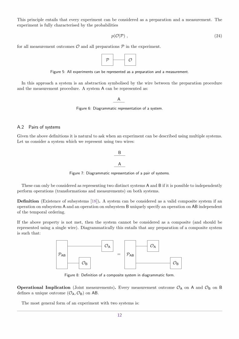
This principle entails that every experiment can be considered as a preparation and a measurement. Theexperiment is fully characterised by the probabilities

p(O|P) , (24)

for all measurement outcomes O and all preparations P in the experiment.

P O

Figure 5: All experiments can be represented as a preparation and a measurement.

In this approach a system is an abstraction symbolised by the wire between the preparation procedureand the measurement procedure. A system A can be represented as:

A

Figure 6: Diagrammatic representation of a system.

A.2 Pairs of systems

Given the above definitions it is natural to ask when an experiment can be described using multiple systems.Let us consider a system which we represent using two wires:

A

B

Figure 7: Diagrammatic representation of a pair of systems.

These can only be considered as representing two distinct systems A and B if it is possible to independentlyperform operations (transformations and measurements) on both systems.

Definition (Existence of subsystems [18]). A system can be considered as a valid composite system if anoperation on subsystem A and an operation on subsystem B uniquely specify an operation on AB independentof the temporal ordering.

If the above property is not met, then the system cannot be considered as a composite (and should berepresented using a single wire). Diagrammatically this entails that any preparation of a composite systemis such that:

PAB

OB

OA

= PAB

OB

OA

Figure 8: Definition of a composite system in diagrammatic form.

Operational Implication (Joint measurements). Every measurement outcome OA on A and OB on Bdefines a unique outcome (OA,OB) on AB.

The most general form of an experiment with two systems is:

12

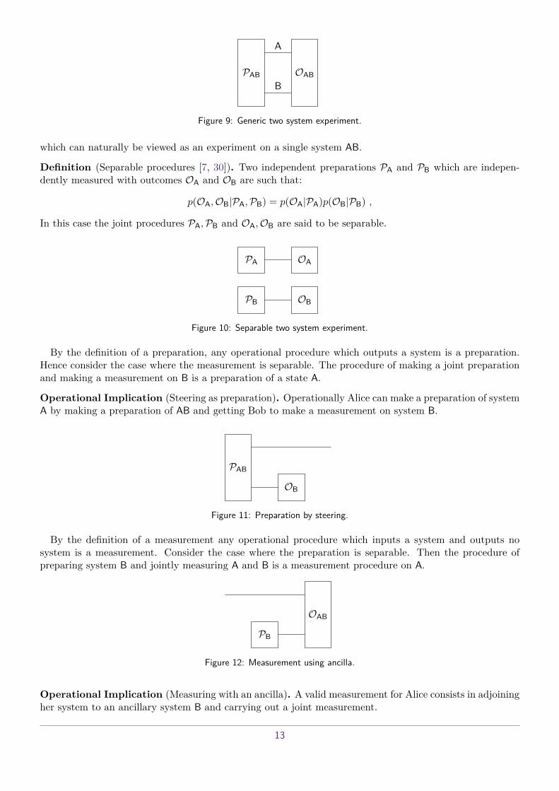
PABBOAB

A

Figure 9: Generic two system experiment.

which can naturally be viewed as an experiment on a single system AB.

Definition (Separable procedures [7, 30]). Two independent preparations PA and PB which are indepen-dently measured with outcomes OA and OB are such that:

p(OA,OB|PA,PB) = p(OA|PA)p(OB|PB) ,

In this case the joint procedures PA,PB and OA,OB are said to be separable.

PB OB

PA OA

Figure 10: Separable two system experiment.

By the definition of a preparation, any operational procedure which outputs a system is a preparation.Hence consider the case where the measurement is separable. The procedure of making a joint preparationand making a measurement on B is a preparation of a state A.

Operational Implication (Steering as preparation). Operationally Alice can make a preparation of systemA by making a preparation of AB and getting Bob to make a measurement on system B.

PAB

OB

Figure 11: Preparation by steering.

By the definition of a measurement any operational procedure which inputs a system and outputs nosystem is a measurement. Consider the case where the preparation is separable. Then the procedure ofpreparing system B and jointly measuring A and B is a measurement procedure on A.

PB

OAB

Figure 12: Measurement using ancilla.

Operational Implication (Measuring with an ancilla). A valid measurement for Alice consists in adjoiningher system to an ancillary system B and carrying out a joint measurement.

13

In the case where both preparation and measurement are separable then the experiment can be viewed astwo separate experiments. In the bi-partite case there are no further methods of generating preparationsand measurements. Hence when determining whether a pair of systems is consistent with the operationalproperties which arise from composition, these are the only features which we need to consider.

One may ask whether any further operational implications will emerge from considering more than twosystems.

Operational Assumption (Associativity of composition). The systems (AB)C and A(BC) are the same.

This implies that there are no new types of procedures which can be carried out on a single system byappending more than one system. Consider an experiment with multiple systems A,B,C.... For any par-titioning of the experiment which creates a preparation of system A, all regroupings of systems B,C, ...are equivalent. This is a preparation by steering of system A conditional on a measurement on systemsB,C, ... which can be viewed as a single system. Diagrammatically it tells us that all ways of partitioningan experiment with multiple systems are equivalent.

This entails the only constraints imposed by the operational framework will come from the assumptionsand implications outlined above. There are no further operational implications which emerge from the abovedefinitions and assumptions.

In the next section we translate the operational features above into the language of OPFs, and show whichconstraints they impose on the OPF sets Fd.

A.3 Consistency constraints

We assume the Finiteness Principle holds, and that for a set of OPFs Fd there exists a finite linearlygenerating set {Fi}Kd

i=1. That is to say:

F =∑i

ciFi . (25)

A.3.1 Constraint C1

Consistency constraint C1 follows directly from the fact that the composition of a transformation and ameasurement is a measurement.

A.3.2 Constraint C2

Definition (State). A state corresponds to an equivalence class of indistinguishable preparation procedures.

From this definition it follows that two states cannot be indistinguishable. This implies C2. In a systemwhere some pure states are indistinguishable the manifold of pure states would no longer be the set of rayson Cd (as required by the first postulate).

A.3.3 Constraint C3

Consider a composite system AB. By the definition of a composite system above, for any OPF FA on Aand FB on B there exists an OPF FA ? FB on AB. By the assumption that mixing is possible, the outcome{pi, F iA} is a valid outcome.

Operational Assumption (Mixing separable procedures). If two parallel processes are separable, it isequivalent to mix them before they are considered as a joint process or after.

From the above assumption it follows that:

(∑i

piFiA) ? FB =

∑i

pi(F iA ? FB) (26)

FA ? (∑i

piFiB) =

∑i

pi(FA ? FiB) (27)

14

If we further assume that it is possible to mix with subnormalised probabilities, i.e.∑i pi ≤ 1 then the ?

product is bi-linear. The identity uA ? uB = uAB follows from the fact that a separable measurement is avalid measurement on AB, and hence:

uAB =∑i,j

(F iA ? FjB) = uA ? uB . (28)

Principle (Uncorrelated pure states). Given two systems A and B independently prepared in pure statesψA and φB the joint state of the system AB is given by ψA ⊗ φB.

This principle, together with the definition of independent systems implies that:

(FA ? FB)(ψA ⊗ φB) = FA(ψA)FB(φB) (29)

A.3.4 Constraint C4

Let us consider the steering scenario. In this case the process of both Alice and Bob making a measurementwith outcome FA ?FB on a joint state φAB can be considered as a measurement with outcome FA on systemA prepared in a certain manner.

An arbitrary preparation of system A is given by {pi, ψiA}. Hence the steering preparation implies that foreach preparation of AB and for each local measurement outcome on B there exists a state {pi, ψiA} in whichsystem A is prepared. In the OPF formalism this means that for every φAB ∈ CdAdB and every FB ∈ FdBthere exists an ensemble {piφiA} such that

(FA ? FB)(φAB)(uA ? FB)(φAB) =

∑i

piFA(ψiA) , (30)

holds for all FA ∈ FdA . The normalisation occurs due to the fact that summing over the measurementoutcomes FA should give unity on both sides of the expression.

A.3.5 Constraint C5

Let us consider the scenario consisting in measuring with an ancilla. In this case Alice and Bob carry out ajoint measurement with outcomes FAB on a system in an uncorrelated state ψA⊗φB. This should correspondto a valid measurement with outcome F ′A on system A prepared in state ψA. For each FAB ∈ FdAdB and foreach φB ∈ CdB there exists an F ′A ∈ FdA such that

FAB(ψA ⊗ φB) = F ′A(ψA) , (31)

for all ψA ∈ CdA .

B Violation of purification

In this appendix we show that all alternative measurement postulates violate purification (for an arbitrarychoice of ancillary system dimension).

As shown in [6] the representations Γd corresponding to alternative measurement postulates for systemswith pure states Cd (d > 2) are of the form

Γ =⊕j∈JDdj , (32)

where J is a list of non-negative integers (at least one of which is not 0 or 1) and Ddj are representations ofSU(d) labelled by Young diagrams (2j, j, . . . , j︸ ︷︷ ︸

d−2

).

15

Consider a system SAB = {CdAdB ,ΓAB} which is the composite of two systems SA = {CdA ,ΓA} andSB = {CdB ,ΓB}. Here the representations Γ are of the form (32). Let us define the following equivalenceclasses of pure global states:

[|ψ〉AB]UB = {|ψ〉′AB ∈ CdAdB | |ψ〉′AB = IA ⊗ UB |ψ〉AB} (33)

All members of the same equivalence class are necessarily mapped to the same reduced state of Alice.Otherwise, Bob could signal to Alice. We note that [26] makes use of this observation in a similar context.Let us call the set of all these equivalence classes RB.

RB := {[|ψ〉AB]UB | |ψ〉AB ∈ CdAdB} (34)

The map from global states to reduced states can be defined on the equivalence classes [|ψ〉AB]UB since twomembers of the same equivalence class are always mapped to the same reduced states. R : RB → SA is themap from equivalence classes to reduced states:

R([|ψ〉AB]UB) = ωA(|ψ〉AB) , (35)

where ωA(|ψ〉AB) is the reduced state obtained in the standard manner from the global state |ψ〉AB (asoutlined in the following appendix). Next we prove that the image of R is smaller than SA for any non-quantum measurement postulates. In other words there are some (local) mixed states in SA which are notreduced states of the global pure states |ψ〉AB.

In the Schmidt decomposition a state |ψ〉AB is:

|ψ〉AB =dA∑i=1

λi |i〉A |i〉B , λi ∈ R ,∑i

λ2i = 1 , (36)

where we assume that the Schmidt coefficients are in decreasing order λi ≥ λi+1. Two states with the samecoefficients and the same basis states on Alice’s side belong to the same equivalence class [|ψ〉AB]UB . Also,two Alice’s basis differing only by phases (e.g. {|i〉A} and {eiθi |i〉A}) give rise to the same equivalence class.Because the phases eiθi can be absorbed by Bob’s unitary.

Let us count the number of parameters that are required to specify an equivalence class in RB. First, wehave the dA − 1 Schmidt coefficients. Second, we note that the number of parameters to specify a basis inCdA is the same as to specify an element of U(dA). Which is the dimension of its Lie algebra, d2

A, the set ofanti-hermitian matrices. Third, we have to subtract the dA irrelevant phases θi. The three terms togethergive

(dA − 1) + d2A − dA = d2

A − 1 (37)

Hence d2A − 1 parameters are needed to specify elements of RB. The set Image(R) requires the same or

fewer parameters to describe as RB. This follows from the fact that every element of RB can be mapped todistinct images, or multiple elements can be mapped to the same image.

Hence by requiring that Alice’s reduced states are in one-to-one correspondence with these equivalenceclasses, her state space must have a dimension d2

A − 1. The only measurement postulates which generate astate space with this dimension are the quantum ones. This follows from the fact that the dimension of theirreducible representations Ddj corresponding to alternative measurement postulates are given by:

Ddj =

( 2jd− 1 + 1

) d−2∏k=1

(1 + j

k

)2, (38)

This is equal to d2−1 for the case j = 1 (corresponding to the quantum state space). Moreover, since this isthe lowest dimensional (non-trivial) such representation there are no reducible representations of the form⊕iDdi which are of dimension d2 − 1.

16

C OPF formalism, representation theory and local tomographyIn this appendix we show that each set of OPFs Fd is associated to a representation of the group SU(d).We also show that the representations associated to locally tomographic systems with sets of OPFs FdAdBhave certain features when restricted to the local subgroup SU(dA)× SU(dB). It is these features which willbe used in the next appendix to show that all non-quantum measurement postulates lead to a violation oflocal tomography. In the following we assume the Finiteness Principle holds.

C.1 Single systems

Lemma 1. To each set of measurement postulates Fd obeying the Finiteness Principle there exists a uniquerepresentation Γd of SU(d) associated to that set.

Proof. We take a set of measurement postulates F , where {Fi} form a basis for F .

F (ψ) =∑i

ciFi(ψ) , ∀ψ . (39)

We consider an OPF F ◦ U :(F ◦ U)(ψ) = F (Uψ) =

∑i

ciFi(Uψ) (40)

WhereFi(Uψ) = (Fi ◦ U)(ψ) =

∑j

Γji (U)Fj(ψ) . (41)

HenceF ◦ U(ψ) =

∑ij

ciΓji (U)Fj(ψ) (42)

Consider

F (UU ′ψ) =∑ij

ciΓji (U)Fj(U ′ψ)

=∑ijk

ciΓji (U)Γkj (U ′)Fk(ψ) (43)

We can also consider UU ′ as a single element:

F (UU ′ψ) =∑ik

ciΓki (UU ′)Fk(ψ) (44)

This shows that Γ(UU ′) = Γ(U)Γ(U ′) and the map Γ : U 7→ Γ(U) is a representation of SU(d).

Lemma 2. The representation Γd of measurement postulates Fd contains a unique trivial subrepresentation.

Proof. Consider a set of OPFs {F (i)} which form a measurement. The OPF u =∑F (i) is such that

u(ψ) = 1 ∀ψ. Consider the basis {Fi} where F1 = u. We observe that u(ψ) = u(Uψ), ∀U ∀ψ. Thisimplies that Γ(U)u = u ∀U and that the representation Γ has a trivial component. If the representationhad another trivial component, it would necessarily be linearly dependent on the first. It would then bea redundant entry in the list of fiducial outcomes which is contrary to the property that they are linearlyindependent.

C.2 Composite systems

The measurement structure FAB contains all measurements of the form FA?FB where FA ∈ FA and FB ∈ FB.Let {F iA} and {F jB} be bases for the two OPF spaces. Then the OPFs F iA ? F

jB form a basis for the global

OPFs FA ? FB. Hence a basis for FAB is {F iA ? FjB, F

kAB} [31, 32].

17

C.2.1 Local tomography

A bi-partite system is locally tomographic if {F iA ? FjB}ij is a basis for RFdAdB .

Lemma 3. For a locally tomographic bi-partite system with representation ΓdAdB the restriction of ΓdAdB

to SU(dA)× SU(dB) is:ΓdAdB|SU(dA)×SU(dB) = ΓdA � ΓdB (45)

Proof. Let us consider the action of an element of SU(dA)× SU(dB) on an OPF FAB =∑ij γij(F iA ⊗ F

jB) in

FAB .

ΓdAdBUA⊗UB

FAB = FAB ◦ (UA ⊗ UB) =∑ij

γij(F iA ⊗ FjB) ◦ (UA ⊗ UB) . (46)

Using the fact that (FA ⊗ FB) ◦ (UA ⊗ UB) = (FA ◦ UA)⊗ (FB ◦ UB):

ΓdAdBUA⊗UB

FAB =∑ij

γij(F iA ◦ UA)⊗ (F jB ◦ UB) . (47)

From the actions of SU(dA) and SU(dB) on RFdA and RFdB we have:

F iA ◦ UA = ΓdAUAF iA , (48)

F jB ◦ UB = ΓdBUBF jB . (49)

Hence,

ΓdAdBUA⊗UB

FAB =∑ij

γij(ΓdAUAF iA ⊗ ΓdB

UBF jB) =

∑ij

γij(ΓdAUA⊗ ΓdB

UB)(F iA ⊗ F lB) = (ΓdA

UA⊗ ΓdB

UB)FAB . (50)

C.2.2 Holistic systems

A bi-partite system which is not locally tomographic is holistic. Real vector space quantum theory is anexample of a holistic theory [33]. A basis for FdAdB in a holistic bi-partite system is {F iA?F

jB, F

kAB}ijk [31, 32].

Here {F iA ? FjB}ij span the locally tomographic subspace of FdAdB denoted FLT

dAdB. Due to bilinearity of the

? product the map ? : RFdA × RFdB → RFLTdAdB

is isomorphic to a tensor product.

Lemma 4. For a holistic bi-partite system with representation ΓdAdB the restriction of ΓdAdB to SU(dA) ×SU(dB) is:

ΓdAdB|SU(dA)×SU(dB) = ΓdA � ΓdB ⊕

⊕i

ΓdAi � ΓdB

i , (51)

where the representations ΓdAdB , ΓdA and ΓdB contain a trivial representation. This is not necessarily thecase for ΓdA

i and ΓdBi (which may not be of the form DdA

j or DdBj ).

Proof. In holistic systems a basis for FAB is {F iA ⊗ FjB, F

kAB}ijk.

FAB =∑ij

γLTij (F iA ⊗ F

jB) +

∑k

γHk F

kAB = FLT

AB + FHAB . (52)

We consider the action of a SU(dA)× SU(dB) subgroup on span({F iA ⊗ FjB}ij).

F iA ⊗ FjB ◦ (UA ⊗ UB) = (F iA ◦ UA)⊗ (F jB ◦ UB) . (53)

The action of SU(dA) × SU(dB) maps basis elements of the form FA ⊗ FB to other elements of that form.Hence span(F iA ⊗ F

jB) is a proper subspace of FAB left invariant under the action of SU(dA)× SU(dB). The

representation ΓdAdB|SU(dA)×SU(dB) is reducible and decomposes as:

ΓdAdB|SU(dA)×SU(dB) = ΓdAdB

LT|SU(dA)×SU(dB) ⊕ ΓdAdBH|SU(dA)×SU(dB) . (54)

The action ΓdAdBLT|SU(dA)×SU(dB) on the locally tomographic subspace is of the form ΓdA � ΓdB (as determined in

the previous lemma). ΓdAdBH|SU(dA)×SU(dB) is an arbitrary representation of SU(dA)× SU(dB) hence of the form⊕

i ΓdAi � ΓdB

i .

18

C.3 Representation theoretic criterion for local tomographyConsider a bi-partite system with alternative measurement postulates FdAdB , FdA and FdB . If the theory islocally tomographic then necessarily:

ΓdAdB|SU(dA)×SU(dB) = ΓA � ΓB (55)

Where ΓA and ΓB both contain a unique trivial representation. By contraposition, any system which hasa representation ΓdAdB

AB which does not have this form when restricted SU(dA) × SU(dB) cannot obey localtomography. This allows us to establish the following test for violation of local tomography:

Lemma 5. Given a bi-partite system with measurement postulates FdAdB , FdA and FdB . The associatedrepresentation are ΓdAdB

AB , ΓdAA and ΓdB

B . If ΓdAdB|SU(dA)×SU(dB) is not of the form (55) then the system is holistic.

C.3.1 Affine representation and existence of trivial times trivial as a criterion

The above lemmas can be translated into the affine representation Γd which do not contain a trivial sub-representation.

Γd = 1d ⊕ Γd . (56)where 1d is the trivial representation of SU(d). We can decompose the tensor product action:

ΓdA � ΓdB = (1dA ⊕ ΓdA) � (1dB ⊕ ΓdB) = (1dA � 1dB)⊕ (1dA � ΓdB)⊕ (ΓdA � 1dB)⊕ (ΓdA � ΓdB) . (57)

The first term occurs due to the trivial component in ΓdAdBAB = 1dAdB ⊕ ΓdAdB

AB .For a locally tomographic system with OPF set FdAdB and representation ΓdAdB , the restriction of ΓdAdB

to the local subgroup SU(dA)× SU(dB), has the following form:

ΓdAdB|SU(dA)×SU(dB) = (1dA � ΓdB)⊕ (ΓdA � 1dB)⊕ (ΓdA � ΓdB) . (58)

This shows that for a locally tomographic theory the representations ΓdAdBAB|SU(dA)×SU(dB) cannot contain any

terms 1dA � 1dB . By contraposition we establish:

Lemma 6. Given a bi-partite system (CdAB ,FdAdB ,ΓdAdB) with subsystems (CdA ,FdA ,ΓdA) and(CdB ,FdB ,ΓdB) then if ΓdAdB

AB has a subrepresentation 1dA � 1dB upon restriction to SU(dA) × SU(dB) thecomposite system is holistic.

D Background representation theoryD.1 BackgroundD.1.1 Young diagram

A Young diagram is a collection of boxes in left-justified rows, where each row-length is in non-increasingorder. The number of boxes in each row determine a partition of the total number of boxes n. This partitiondenoted λ is associated to the Young diagram which is said to be of shape λ. We write |λ| = n for the totalnumber of boxes.

A Young diagram withm rows (labelled 1 tom) where row i has ni boxes (by definition n1 ≥ n2 ≥ ... ≥ nm)is written λ = (n1, n2, ..., nm). By definition: ∑

i

ni = n (59)

λ1 = , λ2 = , λ3 = . (60)

The above Young diagrams are λ1 = (2, 1), λ2 = (3, 3, 2, 1) and λ3 = (5, 2, 1, 1).In the case where a diagram has m multiple rows of the same length l we write lm instead of writing out

“l” m times.. For instance λ2 = (32, 2, 1)

19

D.1.2 Representations of SU(d)

The special unitary group SU(d) is the Lie group of d × d unitary matrices of determinant 1. A finite-dimensional representation of SU(d) is a smooth homomorphism SU(d) → GL(V ), with V a finite-dimensional (complex) vector space.

Irreducible representations of SU(d) are labelled by Young diagrams with at most d rows. There is nolimit on the total number of boxes. A column of d boxes can be removed from a Young diagram of arepresentation of SU(d) without changing the representation labelled by the diagram. Hence an irreduciblerepresentation of SU(d) corresponds to an equivalence class of Young diagrams up to columns of size d.Typically the canonical representative member of the equivalence class is the Young diagram where allcolumns of length d have been removed. With this choice of representative element of each class the Youngdiagram of representations of SU(d) have at most d−1 rows. For example the equivalence class of rectangularYoung diagrams of columns of length d are all mapped to the empty diagram (since all columns are removed).

λ1 = , λ2 = , λ3 = . (61)

These three Young diagrams are equivalent up to columns of length 4. They all label the same represen-tation of SU(4). The canonical representative of the equivalence class is λ3. In the following the expression“representation of SU(d) labelled by the Young diagram λ” is used to mean “representation of SU(d) labelledby the equivalence class of Young diagrams with representative member λ”. The young diagram labelsthe fundamental representation of SU(d). The empty diagram labels the trivial representation.

Given a canonical representative λ we call λf the diagram in the same equivalence class which has f boxes(in other words to which a number of columns of length d have been added such that the total number ofboxes is f). For example λ2 = λ3

8.

Γdλ is the representation of SU(d) associated to the Young diagram λ. The index d will be dropped whenthe context makes it obvious.

D.1.3 Representations of the symmetric group

The symmetric group on n symbols Sn has as group elements all permutation operations on n distinctsymbols. The conjugacy classes of Sn are labelled by partitions of n. Hence the number of (inequivalent)irreducible representations of Sn is the number of partitions of n. Moreover these irreducible representationscan be parametrised by partitions of n. These are labelled by Young diagrams with n boxes [34].

∆nλ denotes the representation of Sn labelled by the Young diagram λ. The index n will be dropped when

the context makes it obvious.

D.2 Branching rule SU(mn)→ SU(m)× SU(n)

D.2.1 Definition

Consider an irreducible representation Γmnλ of SU(mn) and restrict it to a SU(m)× SU(n) subgroup:

Γmnλ (U1 ⊗ U2), ∀U1 ∈ SU(m) ,∀U2 ∈ SU(n) . (62)

In general this will yield a reducible representation of SU(m)× SU(n). This representation will be built ofirreducible representations Γmµ � Γnν

(Γmµ � Γnν )(U1, U2) = Γmµ (U1)⊗ Γnν (U2) , (63)

We write Γmnλ|SU(m)×SU(n) for the restriction of Γmnλ to a SU(m)× SU(n) subgroup. In general:

Γmnλ|SU(m)×SU(n) =⊕µ,ν

Γmµ � Γnν , (64)

20

Where there can be repeated copies for a given µ, ν. In general finding which representations Γmµ �Γnν occurin this restriction is a hard problem. In the following we outline a method which allows us to determine themultiplicity of Γmµ � Γnν in Γmnλ|SU(m)×SU(n). λ , µ and µ will refer to the Young diagrams of Γmnλ , Γmµ and Γnνrespectively.

D.2.2 Inner product of representations of the symmetric group

We consider two representations ∆µ and ∆ν of Sf . We construct the Kronecker product of the two matrices∆µ(s) and ∆ν(s) for all s ∈ Sf . This creates a representation which we call the tensor product ∆µ ⊗ ∆ν

(sometimes called the inner product). In general this is a reducible representation:

∆µ ⊗∆ν =⊕λ

g(µ, ν, λ)∆λ (65)

Here we abuse notation slightly to mean that g(µ, ν, λ) is the multiplicity of ∆λ in ∆µ⊗∆ν . These g(µ, ν, λ)are known as the Clebsch-Gordan coefficients of the symmetric group, and understanding them remains oneof the main open problems in classical representation theory. These coefficients are also relevant in quantuminformation theory, as they are related to the spectra of statistical operators [35].

D.2.3 Recipe

What is the multiplicity of Γmµ � Γnν in the restriction of Γmnλ to SU(m) × SU(n)? We adopt the approachfrom [36] to answer this question. Let f = |λ| be the number of boxes in the Young diagram λ. As shown

above λ also labels a representation of the symmetric group on f objects Sf . This representation is ∆fλ.

Take the Young diagram µ (ν) and add columns of m (n) boxes to the left until it has f boxes. The tableauobtained which we call µf (νf ) labels a representation of Sf denoted ∆f

µf(∆f

νf). We remember that adding

columns to the left of length m (n) keeps µ (ν) within the equivalence class of Young diagrams labelling therepresentation Γmµ (Γnν ). Hence µf (νf ) labels the same representation of SU(m) (SU(n)) as µ (ν).

Hence the diagrams λ , µf and νf refer both to representations of the special unitary group Γmnλ ,

Γmµ (= Γmµf) and Γnν (= Γnνf

) as well as representations of Sf : ∆fλ, ∆f

µfand ∆f

νf.

Theorem 1. Γmµ � Γnν occurs as many times in the restriction of Γmnλ to SU(m) × SU(n) as ∆fλ occurs in

∆fµf⊗∆f

νf, where f = |λ| [36].

D.3 Inductive lemma

Lemma 7. Consider representations Γmnλ

, Γmµ , Γnν , Γmnλ , Γmµ , Γnν , Γmnλ′ , Γmµ′ and Γnν′ where λ = λ + λ′,µ = µ+ µ′ ν = ν + ν ′ and |λ|−|µ|m , |λ|−|ν|n , |λ

′|−|µ′|m and |λ

′|−|ν′|n are integers. If Γmnλ|SU(m)×SU(n) contains a term

Γmµ � Γnν and Γmnλ′|SU(m)×SU(n) contains a term Γmµ′ � Γnν′ then Γmnλ|SU(m)×SU(n) contains a term Γmµ � Γnν .

Proof. Γmnλ|SU(m)×SU(n) containing a term Γmµ � Γnν implies that ∆fλ occurs in ∆f

µf⊗ ∆f

νf(by Theorem 1).

Here µf is the tableau µ (ν) to which f−|µ|m (f−|ν|n ) columns of length m (n) has been added so that the total

number of boxes |µf | = f (|νf | = f).

µf = µ+((

f − |µ|m

)m), (66)

νf = ν +((

f − |ν|n

)n). (67)

Here we recall that ((f−|µ|m )m) indicates m rows of length ((f−|µ|m ). This implies that g(λ, µf , νf ) > 0.Similarly g(λ′, µ′f ′ , ν ′f ′) > 0.

We now show that µ = µ+ µ′ and ν = ν + ν ′ implies that µf = µf + µ′f ′ and νf = νf + ν ′f ′ .

21

µf + µ′f ′ = µ+ µ′ +((

f − |µ|m

)m)+((

f ′ − |µ′|m

)m)(68)

= µ+(((f + f ′ − |µ| − |µ′|)

m

)m)(69)

= µ+((

f − |µ|m

)n)= µf . (70)

And similarly for ν.Let us make use of a property of the Clebsch Gordan coefficients called the semi-group property. If

g(λ, µf , νf ) > 0 and g(λ′, µ′f ′ , ν ′f ′) > 0 then g(λ+λ′, µf +µ′f ′ , νf +ν ′f ′) > 0 [37]. By the semi-group propertywe have g(λ, µf , νf ) > 0. This implies that ∆f

λoccurs in ∆f

µf⊗ ∆f

µf. By Theorem 1 this implies that

Γmnλ|SU(m)×SU(n) contains a term Γmµ � Γmν .

E Violation of local tomography in all alternative measurement postulatesIn the following we establish that Γ9

|SU(3)×SU(3) is not of the form (58) for all representations Γ9 of SU(9) cor-

responding to non quantum state spaces with pure states C9. We show explicitly that every such restrictioncontains a term of 13 � 13, where 13 is the trivial representation of SU(3).

E.1 Arbitrary dimension d

We now construct a proof by induction to show that the representations Ddj are not compatible with local

tomography when restricted to SU(dA)× SU(dB). A representation Ddj will violate local tomography if it is

not of the form (58) when restricted to SU(dA)× SU(dB). It suffices to show that there is a term 1dA � 1dB

in this restriction in order to show that it is not of this form.

Lemma 8. If the representations Ddj and Dd2 of SU(d) contain a term 1dA �1dB when restricted to SU(dA)×SU(dB) then so does Ddj+2

Proof. Let

Γdλ = Ddj , ΓdAµ = 1dA , ΓdB

ν = 1dB (71)

Γdλ′ = Dd2 , ΓdAµ′ = 1dA , ΓdB

ν′ = 1dB (72)

Γλ = Ddj+2, Γµ = 1dA , ΓdBν = 1dB , (73)

where

λ = (2j, jd−2), µ = 0, ν = 0 , (74)λ′ = (4, 2d−2), µ′ = 0, ν ′ = 0 , (75)λ = (2j + 4, (j + 2)d−2), µ = 0, ν = 0 . (76)

We observe

λ = λ+ λ′, µ = µ+ µ′, ν = ν + ν ′ (77)f = |λ| = jd, f ′ = |λ′| = 2d, f = |λ| = d(j + 2) (78)

Next we check that the quantities below are integer valued:

22

|λ| − |µ|m

= jd

dA= jdB , (79)

|λ| − |ν|n

= jd

dB= jdA , (80)

|λ′| − |µ′|m

= 2ddA

= 2dB , (81)

|λ′| − |ν ′|n

= 2ddB

= 2dA . (82)

From Lemma 7 it follows that if Ddj contains a representation 1dA � 1dB and Dd2 contains a representation1dA � 1dB when restricted to SU(dA)×SU(dB) then Ddj+2 contains a representation 1dA � 1dB when restrictedto SU(dA)× SU(dB).

Hence it suffices to show that Dd2 and Dd3 contain 1dA � 1dB when restricted to SU(dA)× SU(dB) to showthat Ddj does for any j > 1.

E.2 Existence of 13 � 13 for all non-quantum representations of SU(9)

Using Sage software [38] we can show that D92 and D9

3 have a representation 13 � 13 when restricted toSU(3)× SU(3). By Lemma 8 all representations D9

j , j > 1 have this property. An arbitrary representationcorresponding to an alternative Born rule for C9 is of the form:

Γ9 =⊕j∈JD9j (83)

Where J is a list of positive integers containing at least one integer which is not 1. Since at least one (non-trivial) subrepresentation in Γ9 has a 13 � 13 when restricted to SU(3) × SU(3) so does the representationΓ9.

E.3 Violation of local tomography for all theories

Every representation Γ9 of SU(9) of the form (83) has a representation 13 � 13 when restricted to SU(3)×SU(3). It follows from this that the restriction of Γ9 to SU(3)× SU(3) is not of the form required for localtomography. From this it follows that all non-quantum C9 systems which are composites of two C3 systemsviolate local tomography.

In order to show that a theory with systems Cd (for every d > 1) violates local tomography, it is sufficientto show that one of the systems in the theory violates local tomography. Since all C9 non-quantum systemsviolate local tomography it follows that all non-quantum theories with systems Cd violate local tomography.We emphasise that here we consider theories for which all values of d > 1 are possible.

F Composition in GPTs

In the earlier appendices we gave a certain primacy to the space of OPFs, and considered the group actionon the linear space spanned by the OPFs. However it is equally valid (and more common) to give primacy tothe space of states and consider the group action on this space. This standard representation will be helpfulfor proving the consistency of the toy model. Indeed the consistency constraints required for compositiontranslate naturally to the language of states. This section is largely without proof, as the proofs carry overnaturally from the OPF formalism to the standard state formalism. We refer the reader to [32] for moredetailed proofs.

23

F.1 Representation of statesThe set of mixed states span a real vector space. A state is a vector:

ω =

F1(ω)F2(ω)

...FKd

(ω)

, (84)

An arbitrary F ∈ Fd can be expressed:F =

∑i

ciFi (85)

To each F we can associate a dual vector (or effect) EF

EF = (c1, ..., cKd) , (86)

By definition EF · ω = F (ω). Let u be effect associated to the unit OPF. Since u · ω = 1 there is a componentfor all states ω which is constant. That is to say we can choose F1 to be the unit OPF:

ω =(

1ω

), (87)

The group representation Γd acting on the state space is of the form Γd = 1d + Γd (Γd may be reducible orirreducible). We can write

EF · ω = c1 + EF · ω (88)In the representation where the trivial component is removed (by an affine transformation) then states

are ω (whose fiducial outcomes are affinely independent), the group representation is Γd and outcomeprobabilities are affine functions EF of the state ω. We observe that from the uniqueness of the trivialcomponent in Γd it follows that Γd cannot contain any trivial subrepresentation.

F.2 Local tomographyConsider measurement postulates FdAdB , FA and FB. States for Alice and Bob can be written as:

ωA =

F 1

A(ωA)F 2

A(ωA)...

FKdAA (ωA)

, (89)

and

ωB =

F 1

B(ωB)F 2

B(ωB)...

FKdBB (ωB)

. (90)

Definition (Local tomography). A composite system SAB is locally tomographic if it has fiducial outcomes{(F iA ? F

jB)}i=KdA ,j=KdB

i=1,j=1 . A state of the composite system can be written:

ωAB =

(F 1

A ? F1B)(ωAB)

(F 1A ? F

2B)(ωAB)...

(FKdAA ? F

KdBB )(ωAB)

, (91)

We observe that EF i

A?FjB

= EF iA⊗ E

F jB. Indeed any joint local effect EFA?FB = EFA ⊗ EFB . Product states

are of the form ωA ⊗ ωB.

24

F.3 Non-locally-tomographic theoriesThe states of a composite system SAB of a non-locally tomographic (or holistic) theory can be writtenas [31, 32]:

ωAB =(λABηAB

), (92)

where

λAB =

(F 1

A ? F1B)(ωAB)

(F 1A ? F

2B)(ωAB)...

(FKdAA ? F

KdBB )(ωAB)

, (93)

is the locally tomographic part and

ηAB =

F 1

AB(ωAB)...

FKdAdB−KdAKdBAB (ωAB)

, (94)

is the holistic part. The probability for a joint outcome FA ? FB is given by:

(FA ? FB)(ωAB) = (EFA ⊗ EFB) · λAB (95)

Joint local effects are computed using the locally tomographic part of the state space only.

F.4 The reduced state spaceThe reduced states for Alice and Bob can be computed as follows:

ωA = (ΓdA(IA)⊗ uB)λAB (96)ωB = (uA ⊗ ΓdB(IB))λAB (97)

Reduced states are determined using only the locally tomographic part of the global state.

G Toy modelIn this appendix we show that the toy model introduced in section 4 meets consistency constraints C1 -C5 (apart from associativity of the ? product).

G.1 Constraints C1 and C2It is immediate that consistency constraints C1 and C2 are met by the toy model.

G.2 Constraint C3We prove (FA ? FB)(ψA ⊗ φB) = FA(ψA)FB(φB) :

(FA ? FB)(ψA ⊗ φB)

= tr(|ψ〉〈ψ|⊗2

A |φ〉〈φ|⊗2B (FAFB + tr(FAFB)

tr(SASB)AAAB))

=tr(|ψ〉〈ψ|⊗2

A |φ〉〈φ|⊗2B FAFB

)= FA(ψA)FB(φB) . (98)

In the penultimate line we have used the fact that the overlap of product states |ψ〉〈ψ|⊗2A |φ〉〈φ|

⊗2B and AAAB

is 0.

25

G.3 Constraint C4In the following it will occasionally useful to label the two copies of CdA with 1 and 3 and to label thetwo copies of CdB with 2 and 4. We write SA for the normalised projector onto the symmetric subspace of(CdA)⊗2. We make use of the identity S = 1

2(I + SWAP) throughout this section.In this section we show that normalised conditional states for Alice are valid states of a CdA system. We

first show this for the specific case where the state is conditioned on the unit effect, i.e. is a reduced state.A reduced state of Alice for a bi-partite system in pure state |ψAB〉〈ψAB|⊗2 is:

ωA = trB(SB|ψAB〉〈ψAB|⊗2

)+ SA

trSAtrAB

(AAAB|ψAB〉〈ψAB|⊗2

). (99)

We show that these reduced states lie in the convex hull of |ψA〉〈ψA|⊗2.

Lemma 9. SB |ψAB〉⊗2 = SASB |ψAB〉⊗2

Proof.|ψAB〉⊗2 = αi1i2αi3i4 |i1i2i3i4〉 . (100)

SB |ψAB〉⊗2 = 12αi1i2αi3i4(|i1i2i3i4〉+ |i1i4i3i2〉) . (101)

Let us relabel i1 ↔ i3 in the last term:

SB |ψAB〉⊗2 = 12(αi1i2αi3i4 |i1i2i3i4〉+ αi3i2αi1i4 |i3i4i1i2〉) . (102)

SASB |ψAB〉⊗2 = 14αi1i2αi3i4(|i1i2i3i4〉+ |i1i4i3i2〉+ |i3i2i1i4〉+ |i3i4i1i2〉) . (103)

Let us relabel i1 ↔ i3 in the second term , i2 ↔ i4 in the penultimate term and i1 ↔ i3 and i2 ↔ i4 in thelast term :

SASB |ψAB〉⊗2 = 14(αi1i2αi3i4 |i1i2i3i4〉+ αi3i2αi1i4 |i3i4i1i2〉 (104)

+αi1i4αi3i2 |i3i4i1i2〉+ αi1i2αi3i4 |i1i2i3i4〉) = 12(αi1i2αi3i4 |i1i2i3i4〉+ αi3i2αi1i4 |i3i4i1i2〉) . (105)

From the above lemma we can write a reduced state ω:

ωA = trB(SASB|ψAB〉〈ψAB|⊗2

)+ SA

trSAtrAB

(AAAB|ψAB〉〈ψAB|⊗2

). (106)

Lemma 10. The reduced state ωA can be written as:

ωA = SA(ρA ⊗ ρA)SA + (1− tr(SA(ρA ⊗ ρA)SA))SA , (107)

where ρA = trB(|ψ〉〈ψ|AB).

Proof. We first show that:trB(SASB|ψ〉〈ψ|⊗2

AB) = SA(ρA ⊗ ρA)SA . (108)

From the proof of Lemma 9:

SASB |ψAB〉⊗2 = 14αi1i2αi3i4(|i1i2i3i4〉+ |i1i4i3i2〉+ |i3i2i1i4〉+ |i3i4i1i2〉) . (109)

Hence:

SASB|ψAB〉〈ψAB|⊗2 =14αi1i2αi3i4αj1b1αj3b2(|i1i2i3i4〉〈j1j2j3j4| (110)

+|i1i4i3i2〉〈j1j2j3j4|+ |i3i2i1i4〉〈j1j2j3j4|+ |i3i4i1i2〉〈j1j2j3j4|) . (111)

26

which implies:

trB(SASB|ψ〉〈ψ|⊗2AB) = 1

2αi1b1αi3b2αj1b1αj3b2(|i1i3〉〈j1j3|+ |i3i1〉〈j1j3|) . (112)

We now compute SA(ρA ⊗ ρA)SA.

|ψ〉〈ψ|AB = αi1i2αj1j2 |i1i2〉〈j1j2| . (113)

ρA = trB(|ψ〉〈ψ|AB) = αi1b1αj1b1 |i1〉〈j1| . (114)

ρA ⊗ ρA = αi1b1αi3b2αj1b1αj3b2 |i1i3〉〈j1j3| . (115)

SA(ρA ⊗ ρA) = 12αi1b1αi3b2αj1b1αj3b2(|i1i3〉〈j1j3|+ |i3i1〉〈j1j3|) . (116)

SA(ρA ⊗ ρA)SA =14αi1b1αi3b2αj1b1αj3b2(|i1i3〉〈j1j3|+ |i3i1〉〈j1j3|) (117)

+14αi1b1αi3b2αj1b1αj3b2(|i1i3〉〈j3j1|+ |i3i1〉〈j3j1|) . (118)

In the second term we relabel j1 ↔ j3, i1 ↔ i3 and b1 ↔ b2 to obtain:

SA(ρA ⊗ ρA)SA = 12(αi1b1αi3b2αj1b1αj3b2(|i1i3〉〈j1j3|+ |i3i1〉〈j1j3|)) . (119)

Hence,

ωA = SA(ρA ⊗ ρA)SA + (1− tr(|ψ〉〈ψ|⊗2ABSASB))SA

= SA(ρA ⊗ ρA)SA + (1− tr(SA(ρA ⊗ ρA)SA))SA . (120)

Lemma 11. The reduced states ωA belong to the convex hull of the local pure states |ψ〉〈ψ|⊗2.

Proof. By Lemma 10 the reduced state can be written as:

ωA = SA(ρA ⊗ ρA)SA + (1− tr(SA(ρA ⊗ ρA)SA))SA , (121)

where ρA = trB(|ψ〉〈ψ|AB). In the following we drop the A label.

ρ =∑i

αi|i〉〈i| , (122)

Here the |i〉 are not necessarily orthogonal. The trace of ρ is∑i αi = 1, where αi > 0. Let us write

Φij = 1√2(|i, j〉+ |j, i〉) and observe:

∑i 6=j|Φij〉〈Φij | = 2

∑i<j

|Φij〉〈Φij | =∑i 6=j

(|i, j〉〈i, j|+ |i, j〉〈j, i|) . (123)

Consider the (not necessarily normalised) matrix

S(ρ⊗ ρ)S = S(∑ij

αiαj |i, j〉〈i, j|)S =∑i

α2i |i, i〉〈i, i|+

∑i<j

αiαj |Φij〉〈Φij | , (124)

The trace of this matrix is 1−∑i<j αiαj ; hence:

ω =∑i

α2i |i, i〉〈i, i|+

∑i<j

αiαj |Φij〉〈Φij |+∑i<j

αiαjS . (125)

27

We now show that this arbitrary mixed state ω can be expressed as a convex combination of local purestates |ψ〉〈ψ|⊗2. Consider the general vector

|ψ〉 =∑i

eiθj√αj |j〉 , (126)

where αj ≥ 0 and for all j. Normalisation implies∑j αj = 1. Now, let us write the pure product state

|ψ〉〈ψ|⊗2 =∑

j,k,j′,k′

eiθjeiθke−iθj′e−iθk′√αjαkαj′αk′ |j, k〉〈j′, k′| . (127)

Let us make the following observations. When j 6= j′:∫ π

−πe−iθjeiθj′dθjdθj′ = 0 . (128)

When j = j′: ∫ π

−πe−iθjeiθj′dθjdθj′ = (2π)2 . (129)

Now consider:

Eθi|ψ〉〈ψ|⊗2 = 1

(2π)4

∫ π

−π

∑j,k,j′,k′

eiθjeiθke−iθj′e−iθk′√αjαkαj′αk′ |j, k〉〈j′, k′|dθjdθkdθj′dθk′ . (130)

The non zero contributions will arise from the following terms:j = j′ = k = k′: ∫ π

−π|eiθj |4dθjdθkdθj′dθk′ = (2π)4 . (131)

j = j′ 6= k = k′: ∫ π

−π|eiθj |2|eiθk |2dθjdθkdθj′dθk′ = (2π)4 . (132)

j = k′ 6= k = j′: ∫ π

−π|eiθj |2|eiθk |2dθjdθkdθj′dθk′ = (2π)4 . (133)

All other contributions will be zero.Now, we write the mixed state corresponding to the uniform average over all values of the phases θi,

ω1 = Eθi|ψ〉〈ψ|⊗2 =

∑j,k

αjαk|j, k〉〈j, k|+∑j 6=k

αjαk|j, k〉〈k, j| , (134)

where the first term arises from contributions (131) and (132) and the second term arises from contribu-tion (133). Then we can write

ω1 =∑i

α2i |i, i〉〈i, i|+ 2

∑i<j

αiαj |Φij〉〈Φij | , (135)

Let us take the state:ω2 =

∑i

α2i |i, i〉〈i, i|+ 2

∑i<j

αiαjS . (136)

This is a mixture of states of the form |ψ〉〈ψ|⊗2 since S =∫|ψ〉〈ψ|⊗2dψ and

∑i α

2i + 2

∑i<j αiαj = 1. If we

take the mixture 12(ω1 + ω2) we obtain (125).

We now consider the more general case where Alice’s state is conditioned on an arbitrary effect FB. Theconditional state for Alice given one of Bob’s effects FB is:

ωA|FB = TrB(SAFB|ψ〉〈ψ|⊗2AB) + Tr(|ψ〉〈ψ|⊗2

ABAAAB)Tr(FB)Tr(SB) SA . (137)

Although effects of the form FB = |φ〉〈φ|⊗2 are not valid (since the complement effects would not be of therequired form), we calculate the conditional state for such effects, as this will allow us to later determineconditional states for general effects FB =

∑i αi|φi〉〈φi|⊗2.

28

Lemma 12. For FB = |φ〉〈φ|⊗2:

TrB(SAFB|ψ〉〈ψ|⊗2AB) = SA(ρψA|φ ⊗ ρ

ψA|φ)SA = ρψA|φ ⊗ ρ

ψA|φ , (138)

where ρψA|φ = Tr((IA ⊗ |φ〉〈φ|B)|ψ〉〈ψ|AB) .

Proof.

TrB(SAFB|ψ〉〈ψ|⊗2AB) = SATrB(FB|ψ〉〈ψ|⊗2

AB) = SA(ρψA|φ ⊗ ρψA|φ) . (139)

Let

ρψA|φ = Tr((IA ⊗ |φ〉〈φ|B)|ψ〉〈ψ|AB

)=∑i1,j1

αi1,φαj1,φ|i1〉〈j1| . (140)

We assume without loss of generality that |φ〉 is one of the basis vectors |i〉.

ρψA|φ ⊗ ρψA|φ =

∑i1,i3,j1,j3

αi1,φαj1,φαi3,φαj3,φ|i1i3〉〈j1j3| . (141)

SA(ρA|φ ⊗ ρA|φ) =12(

∑i1,i3,j1,j3

αi1,φαj1,φαi3,φαj3,φ|i1i3〉〈j1j3|

+∑

i1,i3,j1,j3

αi1,φαj1,φαi3,φαj3,φ|i3i1〉〈j1j3|) . (142)

We relabel i1 ↔ i3 on the last line to obtain SA(ρA|φ ⊗ ρA|φ) = (ρA|φ ⊗ ρA|φ).

SA(ρA|φ ⊗ ρA|φ)SA = 14(

∑i1,i3,j1,j3

αi1,φαj1,φαi3,φαj3,φ|i1i3〉〈j1j3|

+∑

i1,i3,j1,j3

αi1,φαj1,φαi3,φαj3,φ|i3i1〉〈j1j3|+∑

i1,i3,j1,j3

αi1,φαj1,φαi3,φαj3,φ|i1i3〉〈j3j1|

+∑

i1,i3,j1,j3

αi1,φαj1,φαi3,φαj3,φ|i3i1〉〈j3j1|) . (143)

We relabel j1 ↔ j3 on the last two lines to obtain SA(ρA|φ ⊗ ρA|φ) = SA(ρA|φ ⊗ ρA|φ)SA.

We need one more lemma before proving that normalised conditional states belong to the convex hull ofthe local pure states |ψ〉〈ψ|⊗2

A .

Lemma 13. If S(ρ⊗ ρ)S = ρ⊗ ρ with Tr(ρ) = 1 then ρ⊗ ρ =∑i pi|ψi〉〈ψi|⊗2.

Proof. By Lemma 11 this is a valid reduced state and belongs to conv(|ψ〉〈ψ|⊗2).

We observe that since all pure states are such that S(|ψ〉〈ψ|⊗2)S = |ψ〉〈ψ|⊗2 and Tr(|ψ〉〈ψ|⊗2) = 1, we cancharacterise the state space of the systems of the toy model as being given by conv(ρ⊗ ρ) for all normaliseddensity operators such that S(ρ⊗ ρ)S = ρ⊗ ρ.

Lemma 14. The normalised conditional states ωA|FB belong to the convex hull of the local pure states|ψ〉〈ψ|⊗2.

Proof. We first show that the conditional state is a valid local state for effects FB = |φ〉〈φ|⊗2. As a conditionalstate, this state can be subnormalised.

ωA|FB = TrB(SAFB|ψ〉〈ψ|⊗2AB) + cSA , (144)

29

where c = Tr(|ψ〉〈ψ|⊗2ABAAAB)Tr(FB)

Tr(SB) . By Lemma 12 we have the equivalence:

TrB(SAFB|ψ〉〈ψ|⊗2AB) = (ρψA|φ ⊗ ρ

ψA|φ) . (145)

The normalised conditional state is:ωA|FB =

ωA|FB

Tr(ωA|FB) . (146)

Let us set e = Tr(ωA|FB) and d = Tr(SAFB|ψ〉〈ψ|⊗2AB) = Tr(ρψA|φ ⊗ ρ

ψA|φ); e = c+ d.

ωA|FB = 1e

(ρA|φ ⊗ ρA|φ) + c

eSA . (147)

We use the equality ρψA|φ ⊗ ρψA|φ = d(ρψA|φ ⊗ ρ

ψA|φ) where ρψA|F is a standard normalised quantum conditional

state.

ωA|FB =d

e(ρψA|φ ⊗ ρ

ψA|φ) + c

eSA . (148)

By Lemma 12 ρψA|φ ⊗ ρψA|φ = SA(ρψA|φ ⊗ ρ

ψA|φ)SA hence by Lemma 13 it is a valid normalised state (i.e. of

the form∑i pi|ψi〉〈ψi|⊗2). Since 0 < d

e < 1, 0 < ce < 1 and d+c

e = 1 the above is a convex combination ofρψA|φ ⊗ ρ

ψA|φ and SA which are both valid states. Hence the state ωA|FB is a valid local state.

Let FB =∑αi|φi〉〈φi|⊗2, with αi > 0.

ωA|FB =∑i

αi(TrB(SAFB|φi〉〈φi|⊗2|ψ〉〈ψ|⊗2AB) + Tr(|ψ〉〈ψ|⊗2

ABAAAB) 1Tr(SB) SA)

=∑i

αi((ρψA|φi

⊗ ρψA|φi) + ciSA) . (149)

Let e = tr(ωA|FB) and di = tr(ρψA|φi⊗ ρψA|φi

). We have e =∑i αi(ci + di). From above:

ωA|FB =∑i

αi(die

(ρψA|φi⊗ ρψA|φi

) + cieSA) . (150)

Since 0 < αidie < 1 and 0 <

∑iαicie < 1 and

∑iαi(ci+di)

e = 1 the above is a convex combination of(ρψA|φi

⊗ ρψA|φi) with coefficients αidi

e and the state SA with coefficient∑iαicie .

G.4 Constraint C5In this section we show that every OPFs in FG

dAdBapplied to a product state ψA ⊗ φB has a corresponding

OPF F ′A in FLdA

. Let FAB be an arbitrary effect in FLdAdB

. The corresponding operator is

FAB =∑i

αi|xi〉〈xi|12 ⊗ |xi〉〈xi|34 . (151)

We evaluate it on product states:

FAB(ψA ⊗ φB) =∑i

αiTr(|ψ〉〈ψ|⊗2

A |φ〉〈φ|⊗2B (|xi〉〈xi|⊗2

AB))

=∑i

αiTrA(|ψ〉〈ψ|⊗2A TrB(|φ〉〈φ|⊗2

B (|xi〉〈xi|⊗2AB)))

=∑i

αiTrA(|ψ〉〈ψ|⊗2A SATrB(IA|φ〉〈φ|⊗2

B |xi〉〈xi|⊗2AB))

= TrA(|ψ〉〈ψ|⊗2A (∑i

αi(SA(ρxi

A|φ ⊗ ρxi

A|φ)SA))) . (152)

30

By Lemma 13 (SA(ρxA|φ⊗ρxA|φ)SA is of the form

∑j βj |φj〉〈φj |⊗2 with βj ≥ 0. Hence F ′A = (

∑i αi(SA(ρxi

A|φ⊗ρxi

A|φ)SA) is a valid effect on A as long as its complement is also of the form∑i γi|φi〉〈φi|⊗2. Since the

complement of FAB is of the form∑i αi|xi〉〈xi|12⊗ |xi〉〈xi|34 it follows that the associated effect on A (which

is the complement of F ′A) is of the required form. From this it follows that F ′A is a valid effect. The setFGdAdB

also contains effects FA ? FB which are not necessarily of the form given above. However since theseare product effects they trivially are consistent with C5.

31