Antoine Girard

VAL-AMS Project MeetingApril 2007

Behavioral Metrics forSimulation-based Circuit Validation

Time Domain Properties of Circuits

Use Linear or MetricTemporal Logic

• Transient dynamics analysis:

• Desired performance characteristics:1. Maximum overshoot2. Rise time3. Delay time 4. Settling time5. Constraints on input/states6. Response sensitivity

Time Domain Properties of Circuits

System:

Step input (t > 0):

Steady state at t = 0-:

Property:

from Zhi Han’s PhD Thesis 2005

Computer Aided Techniques forCircuit Validation

• Model based validation of time domain properties of circuits and systems:- Specifications: Temporal Logic Formula.- For a set of possible initial states, inputs and parameters.

• Testing:- Simulate a (large) number of trajectories.- Does each trajectory satisfies the specification ?- No validation proof: notion of coverage.

• Reachability based verification:- Compute the (infinite) set of all possible trajectories.- Does each trajectory satisfies the specification ?- Formal proof.

• Intermediate approach:- Can we build a formal proof from a finite number of trajectories ?

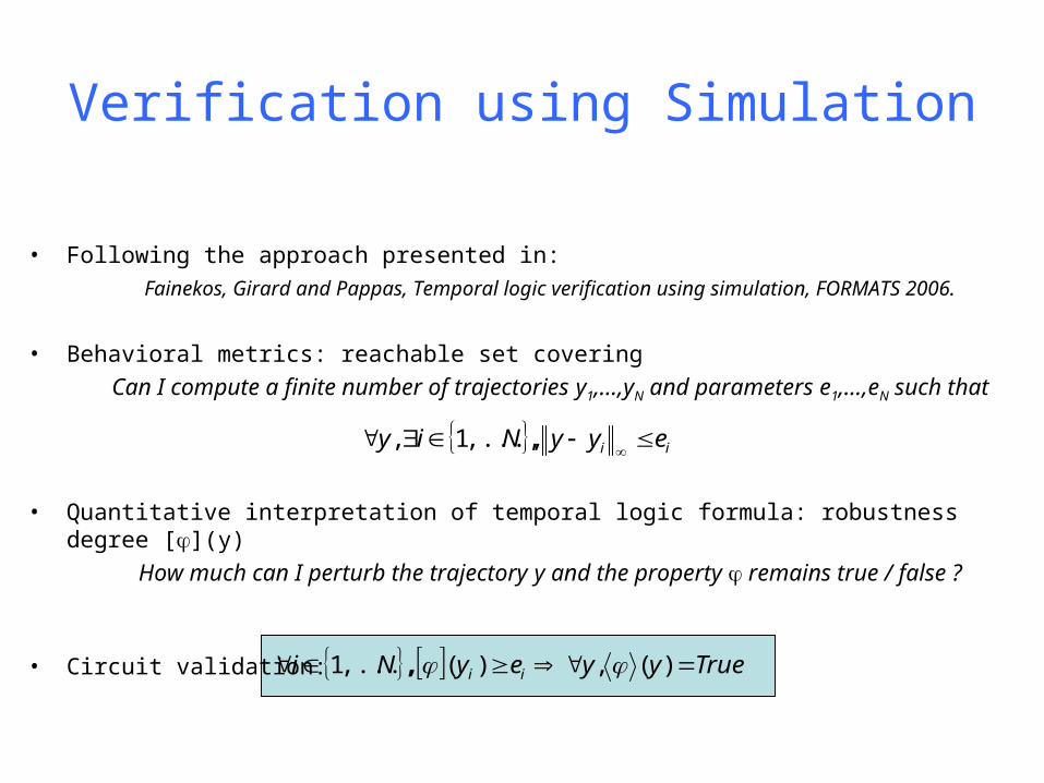
Verification using Simulation

• Following the approach presented in:

Fainekos, Girard and Pappas, Temporal logic verification using simulation, FORMATS 2006.

• Behavioral metrics: reachable set covering

Can I compute a finite number of trajectories y1,…,yN and parameters e1,…,eN such that

• Quantitative interpretation of temporal logic formula: robustness degree [](y)

How much can I perturb the trajectory y and the property remains true / false ?

• Circuit validation:

ii eyyNiy

,,...,1,

TrueyyeyNi ii )(,)(,,...,1

Outline of the Talk

• Behavioral metrics.

• Quantitative interpretation of temporal logics

• Algorithms for circuits validation.

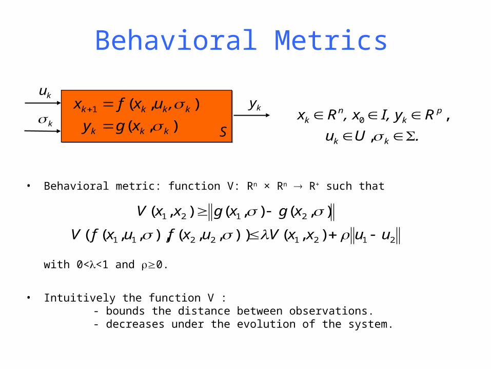
Behavioral Metrics

ky

S),(

),(1

kkk

kkkk

xgy

,uxfx

.Uu

RI, y, xRx

kk

pk

nk

,,0

ku

k

• Discrete time dynamical system with continuous/discrete inputs.

• Distance between trajectories starting from neighbour states, for neighbour sequences of inputs, remains small.

• Notion of behavioral metrics a.k.a.- Contraction metrics (Slotine)- - ISS Lyapunov functions (Angeli)- Bisimulation functions (Girard & Pappas)

Behavioral Metrics

ky

S),(

),(1

kkk

kkkk

xgy

,uxfx

.Uu

RI, y, xRx

kk

pk

nk

,,0

ku

k

• Behavioral metric: function V: Rn × Rn R+ such that

with 0<<1 and 0.

• Intuitively the function V :- bounds the distance between observations.- decreases under the evolution of the system.

21212211

2121

),()),,(),,,((

),(),(),(

uuxxVuxfuxfV

xgxgxxV

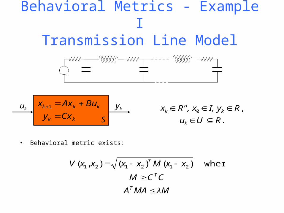
Behavioral Metrics - Example ITransmission Line Model

ky

Skk

kkk

Cxy

BuAxx

1

.

,0

RUu

RI, y, xRx

k

kn

k

ku

• Behavioral metric exists:

MMAA

CCM

xxMxxxxV

T

T

T

where)()(),( 212121

ky

Skk

kk

xCy

BxAx

k

kk

1

2,1

,02

k

kk RI, y, xRx

k

• Behavioral metric exists:

MMAACCM

MMAACCM

xxMxxxxV

TT

TT

T

2222

1111

212121 )()(),(

and

and

where

Behavioral Metrics - Example IIBoost DC/DC Converter

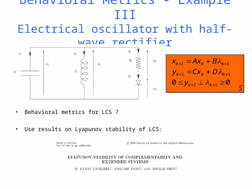
Behavioral Metrics - Example IIIElectrical oscillator with half-wave rectifier

• Behavioral metrics for LCS ?

• Use results on Lyapunov stability of LCS:

00 11

11

11

kk

kkk

kkk

y

DCxy

BAxx

S

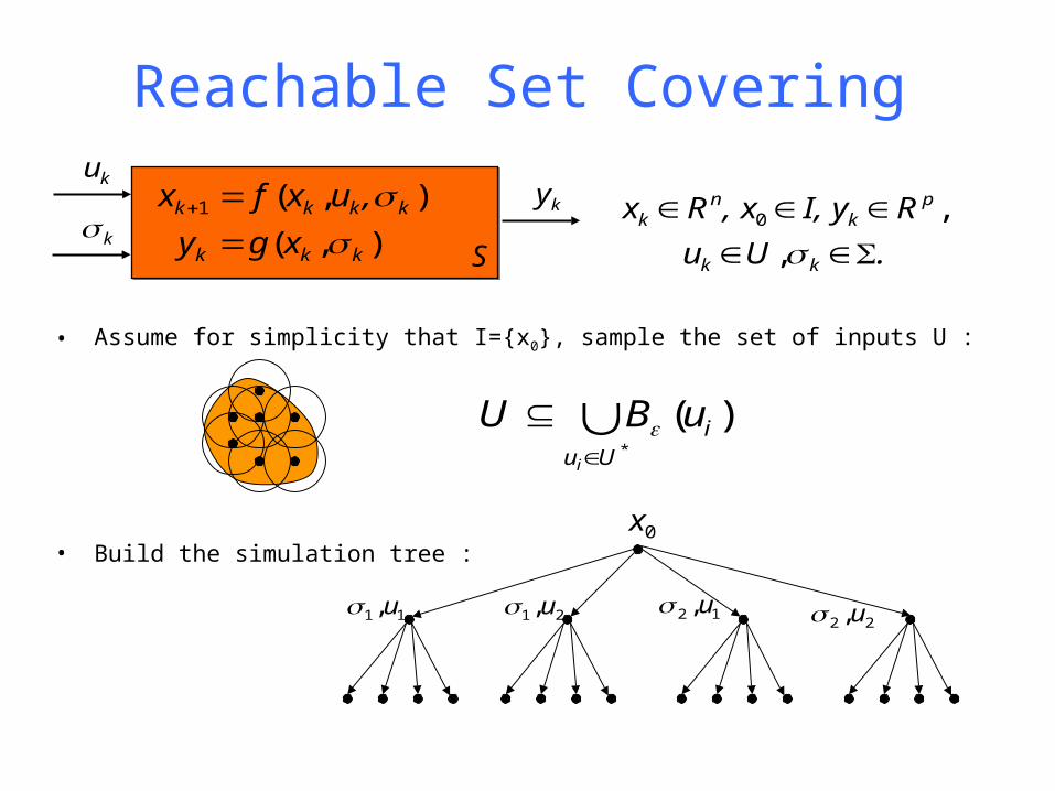
Reachable Set Covering

ky

S),(

),(1

kkk

kkkk

xgy

,uxfx

.Uu

RI, y, xRx

kk

pk

nk

,,0

ku

k

• Assume for simplicity that I={x0}, sample the set of inputs U :

• Build the simulation tree :

*

)(Uu

i

i

uBU

0x

11,u 21,u 12 ,u22 ,u

Reachable Set Covering

ky

S),(

),(1

kkk

kkkk

xgy

,uxfx

.Uu

RI, y, xRx

kk

pk

nk

,,0

ku

k

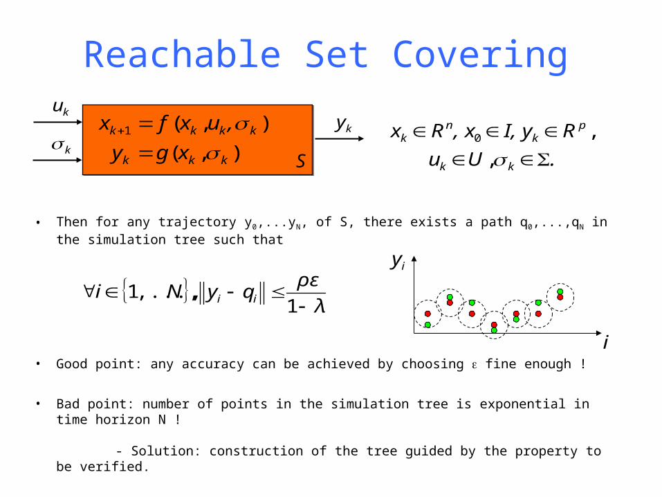
• Then for any trajectory y0,...yN, of S, there exists a path q0,...,qN in the simulation tree such that

• Good point: any accuracy can be achieved by choosing fine enough !

• Bad point: number of points in the simulation tree is exponential in time horizon N !

- Solution: construction of the tree guided by the property to be verified.

λ

ρεqyNi ii

1

,,...,1

i

iy

Outline of the Talk

• Behavioral metrics.

• Quantitative interpretation of temporal logics

• Algorithms for circuits validation.

U uBuAx x'x' x with

Metric Temporal Logic (MTL)

I can be of any bounded or unbounded interval of N.i.e. I = [0,+), I = [2,9]

• Syntax:

• Boolean Semantics:

Fainekos, Pappas: Robustness of Temporal Logic Specifications, 2006

But the Boolean truth value is not enough …

MTL Spec:

((x-10) 2(x10))

MTL Spec:

((x-10) 2(x10))

Fainekos, Pappas: Robustness of Temporal Logic Specifications, 2006

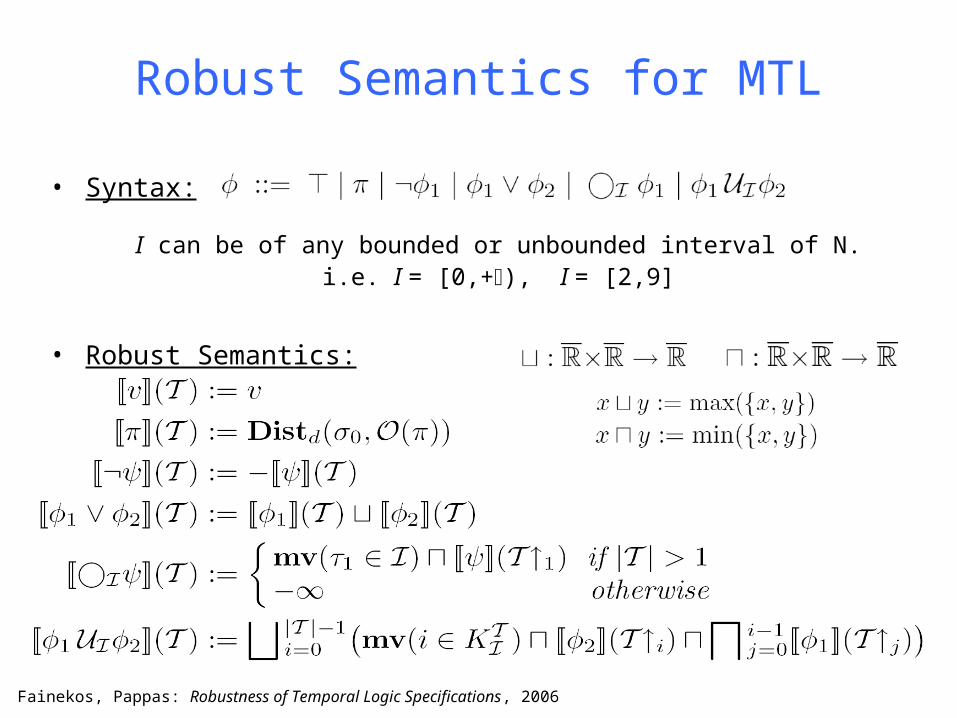
• Syntax:

• Robust Semantics:

Robust Semantics for MTL

I can be of any bounded or unbounded interval of N.i.e. I = [0,+), I = [2,9]

Fainekos, Pappas: Robustness of Temporal Logic Specifications, 2006

Robust and Boolean Semantics for MTL

Proposition: Let Φ be an MTL formula and T be a signal, then

Theorem: Let Φ be an MTL formula and T be a signal, then

N

Fainekos, Pappas: Robustness of Temporal Logic Specifications, 2006

Outline of the Talk

• Behavioral metrics.

• Quantitative interpretation of temporal logics

• Algorithms for circuits validation.

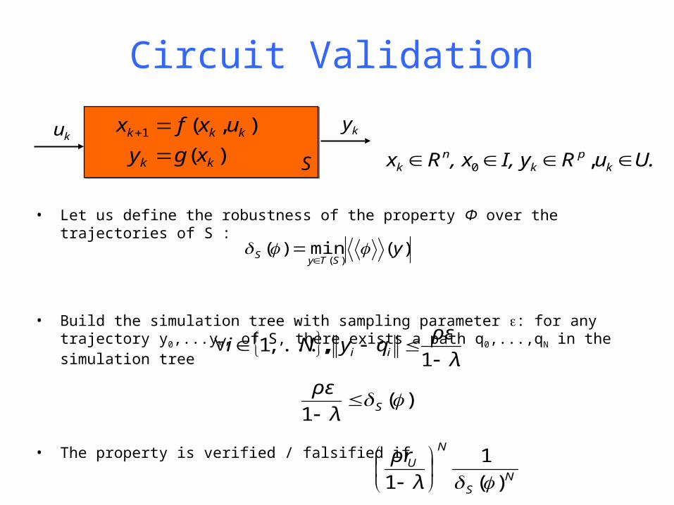
Circuit Validation

ky

S)(

),(1

kk

kkk

xgy

uxfx

U.uRI, y, xRx kp

kn

k ,0

ku

• Let us define the robustness of the property Φ over the trajectories of S :

• Build the simulation tree with sampling parameter : for any trajectory y0,...yN, of S, there exists a path q0,...,qN in the simulation tree

• The property is verified / falsified if

• The number of nodes in the simulation tree is

)(min)()(

ySTy

S

λ

ρεqyNi ii

1

,,...,1

)(1

Sλ

ρε

NS

N

U

λ

ρr

)(

1

1

• The previous algorithm allows to sample uniformly the reachable set

• When interested in property verification, we can adapt locally the sampling to increase efficiency.

• e.g. for safety property:- use coarse sampling when far from the unsafe set- use fine sampling when near the unsafe set

• This multiresolution sampling of the reachable set is obtained by the procedure:

- start with a coarse simulation graph- refine adaptively in regions where it is needed

Property guided Simulation

• Multiresolution simulation graph :

),( 11

00q

),( 11

22q

),( 223 3

q),( 222 2

q

),( 11

11 q

),( 113 3

q

iii

NNN

μ-qy

),μ,(q),,μ(qT(S), ,y,y

that such graph simulation the in

000

Property guided Simulation

• Mark the unsafe states :

),( 11

00q

),( 11

22q

),( 223 3

q),( 222 2

q

),( 11

11 q

),( 113 3

q

Uμ,qN 13

13Π

Uμ,qN 23

23Π Uμ,qN 2

222Π

Uμ,qN 12

12Π

Uμ,qN 10

10Π Uμ,qN 1

111Π

graph simulation the refine to need Otherwise

unsafe, is then , If TUq 12

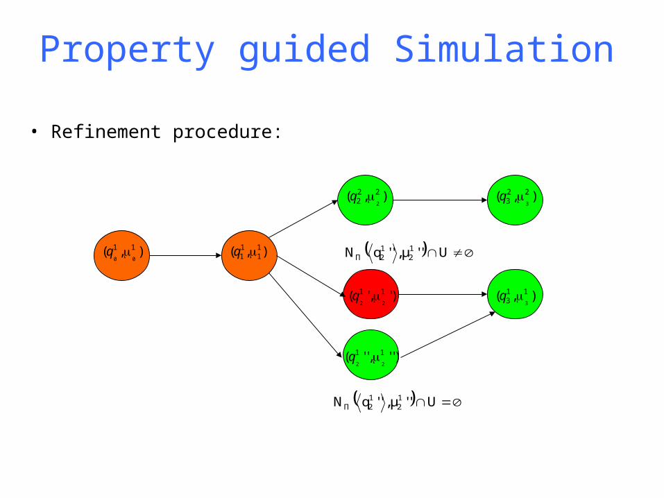
Property guided Simulation

• Refinement procedure:

),( 11

00q

)','( 11

22q

),( 223 3

q),( 222 2

q

),( 11

11 q

),( 113 3

q

)'',''( 11

22q

12

12

12

12 μ'μμ''μ and with

Property guided Simulation

),( 11

00q

)','( 11

22q

),( 223 3

q),( 222 2

q

),( 11

11 q

),( 113 3

q

)'',''( 11

22q

Uμ,qN 12

12Π ''''

Uμ,qN 12

12Π ''''

• Refinement procedure:

Property guided Simulation

),( 11

00q

)','( 11

22q

),( 223 3

q),( 222 2

q

)','( 11

11 q

),( 113 3

q

)'',''( 11

22q

)'',''( 11

11 q

)''','''( 11

22q

• Refinement procedure:

Property guided Simulation

),( 11

00q

)','( 11

22q

),( 223 3

q),( 222 2

q

)','( 11

11 q

),( 113 3

q

)'',''( 11

22q

)'',''( 11

11 q

)''','''( 11

22q

• until you can conclude.

Property guided Simulation

Three-dimensional linear system:

Example

Unsafe = {x2 -7.4} Unsafe = {x2 -7}

Unsafe = {x2 -6.2} Unsafe = {x2 -5.8}

• Verification of infinite state systems using simulation

• Based on the notion of behavioral metrics

• Computational cost related to the robustness of the system- the more robust, the easier the computation- for very robust system, verification requires one simulation

• Future work (in VAL-AMS project)- computation of behavioral metrics for LCS- interface with SICONOS- algorithms for computing “smartly” the simulation tree.- deeper analysis of the computational cost.

Conclusions