Antiproton background rejection in the

Mu2e experimentFrancesco Lucarelli

Abstract

The 8 GeV proton beam hitting a �xed target in the Mu2e experiment has an energy

slightly above the antiproton production threshold; therefore we cannot exclude that some

antiprotons, arising from the interactions between the proton beam and the production

target, propagate through the apparatus, eventually reaching the stopping target and an-

nihilating. The annihilation process may turn out to produce a 105 MeV electron, which

can be mistaken for a signal electron coming from a muon-to-electron conversion. Al-

though possible, the total energy released in an antiproton annihilation is about 2 GeV,whereas in a conversion event it is only 105 MeV; many di�erences can be so found in

the two processes, and the goal of this work is to take advantage of them by developing a

neural network to perform pattern recognition of signal and background events in order to

discriminate between them.

In this work, performed during the stage o�ered by Fermilab to Italian students re-

cruited by the Cultural Association of Italians at Fermilab, I personally analyzed the data

from the simulations of signal and background events in order to eliminate all the back-

ground ones which cannot be mistaken for signals and to choose the best variables to

train the neural network with. The network was then trained through a machine learning

algorithm that I coded in the ROOT environment.

1

2

Contents

1 Introduction 5

1.1 Overview of the experiment . . . . . . . . . . . . . . . . . . . . . . . . . . . . . . 51.2 Apparatus . . . . . . . . . . . . . . . . . . . . . . . . . . . . . . . . . . . . . . . . 61.3 Antiproton background . . . . . . . . . . . . . . . . . . . . . . . . . . . . . . . . 71.4 Neural network and machine learning . . . . . . . . . . . . . . . . . . . . . . . . . 7

1.4.1 Overtraining . . . . . . . . . . . . . . . . . . . . . . . . . . . . . . . . . . 8

2 Selection of the events 9

2.1 Number of tracks . . . . . . . . . . . . . . . . . . . . . . . . . . . . . . . . . . . . 92.2 Track momentum . . . . . . . . . . . . . . . . . . . . . . . . . . . . . . . . . . . . 92.3 Gate time . . . . . . . . . . . . . . . . . . . . . . . . . . . . . . . . . . . . . . . . 92.4 Calorimeter's �rst disk . . . . . . . . . . . . . . . . . . . . . . . . . . . . . . . . . 102.5 Clusters and hits related to the event . . . . . . . . . . . . . . . . . . . . . . . . . 112.6 Particle identi�cation . . . . . . . . . . . . . . . . . . . . . . . . . . . . . . . . . . 12

3 Training variables 13

3.1 Number of clusters and hits . . . . . . . . . . . . . . . . . . . . . . . . . . . . . . 133.2 Clusters and hits time . . . . . . . . . . . . . . . . . . . . . . . . . . . . . . . . . 143.3 Clusters and hits energy . . . . . . . . . . . . . . . . . . . . . . . . . . . . . . . . 143.4 Highest cluster energy . . . . . . . . . . . . . . . . . . . . . . . . . . . . . . . . . 153.5 Clusters center of energy . . . . . . . . . . . . . . . . . . . . . . . . . . . . . . . . 15

4 Neural network training 17

4.1 Output distributions . . . . . . . . . . . . . . . . . . . . . . . . . . . . . . . . . . 174.2 Cut e�ciencies . . . . . . . . . . . . . . . . . . . . . . . . . . . . . . . . . . . . . 174.3 Background rejection and signal e�ciency . . . . . . . . . . . . . . . . . . . . . . 204.4 Importance of variables . . . . . . . . . . . . . . . . . . . . . . . . . . . . . . . . 20

5 conclusions 22

3

Premise

The reported work was performed during the two-month training stage o�ered in summer 2017by Fermilab to Italian students recruited by the Cultural Association of Italians at Fermilab.

As will be described in this report, my supervisor simulated events of conversion electrons(signal) and antiproton annihilations (background), which I then analyzed for two reasons:

• First, I want to get rid of the trivial background events which cannot be mistaken forsignal events, by applying some cuts to the simulated variables;

• Then, I want to choose the best variables to train the neural network with, in order todiscriminate between signal and background events.

These two issues will be discussed respectively in section 2 and section 3, where I willdescribe the problems I faced and the solutions I found. I will also show the plots that I madestarting from the simulated data at disposal.

I then trained a neural network through a machine learning algorithm that I developed inthe ROOT environment of multivariate analysis: all the features of this training and the resultsfrom it will be widely discussed in section 4 and some plots that I realized will make someassertions clearer.

Finally, in section 5 I will describe my observations about the work performed and give somesuggestions to improve it.

4

1 Introduction

1.1 Overview of the experiment

After the discovery of the neutrino oscillations it was clear that the lepton �avor is not strictlyconserved in the elementary processes: the possibility for a muon neutrino to oscillate into anelectron one results in the direct lepton �avor violation (LFV). Although the violation has beenobserved only in the neutral leptons so far (i.e. neutrinos), according to Standard Model (SM)Charged Lepton Flavor Violation (CLFV) must also occur at some level, as shown for examplein the process in �gure 1 [5].

Figure 1: Simple diagram for CLFV in the pro-cess µ→ eγ according to SM. The neutrino os-cillation is necessary for it to occur.

CLFV may also arise in other processes,mostly involving the muon decay, such asµ → eγ, µ → eee or µN → eN (the lastone being the conversion of a muon into anelectron in the �eld of a nucleus N). In anycase, the Standard Model (SM) predicts thecharged lepton �avor violating processes tobe extremely rare: the branching ratio forthe process µ → eγ (�gure 1), as an exam-ple, is about 10−52 [1]. This is why, althoughseveral experiments on CLFV, only a limiton the branching ratio of these processes hasbeen set so far.

The Mu2e experiment will look for the neutrinoless conversions of muons into electrons inthe �eld of an Aluminium nucleus: µN → eN . Since it is a two bodies process, the electronsresulting from the conversions are expected to be monochromatic with an energy [2]

Ee = mµc2 − Ebind − Erecoil = 104.96 MeV

being mµ the muon mass, Ebind its binding energy and Erecoil the nucleus recoil energy. Thepurpose of the experiment is to improve the sensitivity for the CLFV by four orders of magnituderespect to the previous experiments (�gure 2), by measuring the ratio between the rate ofneutrinoless conversions and the rate of the muonic captures [10]:

Rµe =R(µ−N → e−N)

R(µ−N → all muonic nuclear captures)

Mu2e aims to reach a sensitivity of Rµe = 2.5× 10−17: since many Beyond Standard Model(BSM) theories predict a rate Rµe = 10−15 [8], this experiment would provide the su�cientsensitivity to test many of them, and if some conversion electrons are observed, we will beprovided for sure with proof of New Physics [6].

Figure 2: Experiments about CLFV and their sensitivity. Mu2e is expected to improve thesensitivity by four orders of magnitude compared to the previous experiments [5].

5

1.2 Apparatus

Figure 3: Apparatus of the Mu2e experiment.

Figure 3 shows the apparatus of the experiment. A 8 GeV proton beam impinges on a�xed target (production target) and produces many secondary particles (mostly pions) as aconsequence of the interactions arising in the target. Because of the relative orientation betweenthe beam direction and the apparatus, designed to reduce the background in the detectors,the particle momenta are mainly produced in the backward direction: for this reason, a highmagnetic �eld is used in the production solenoid to collect and re�ect the pions towards thetransport solenoid in helical trajectories.

In the transport solenoid, the gradient of the magnetic �eld is responsible for the curvatureof the particle beam and during the �ight almost every pion is expected to decay into a muon.Three collimators permit to select those particles with the desired charge and momentum. Alayer of low Z material is placed in these collimators to stop some of the background sourceparticles (such as antiprotons) [3], thin enough to produce no e�ects on the muons' motion.

Out of the transport solenoid the muons impinge on an Aluminium target (stopping target)where they slow down and eventually interact with the Aluminium nuclei producing muonicatoms, i.e. atoms where an electron is replaced by a muon. These muons are expected to be inthe ground state, or to reach it very quickly from an excited state.

In the nuclei �elds, muons can undergo at least three processes : they can decay in orbit(µ− → e−νµνe), which is a background source, they can be captured (µ−N → νµN

′) or theycan be neutrinoless converted into electrons (µ−N → e−N), which is the signal. Particlesemerging form the stopping target are then detected by a tracker and a calorimeter, whichprovide energy, momentum and time measurements.

Figure 4: The Mu2e tracker (left) and its frontal section (right). In the right picture are alsoshown the projections of the helical trajectories for the signal electrons (green circle) and thebackground ones from the decay-in-orbit (DIO) process (black circles).

The tracker is shown in �gure 4 [3] and is designed to get rid of most of the backgroundelectrons by detecting only those with energies greater than about 53 MeV [2]: infact a signal

6

electron is expected to have ∼ 105 MeV of energy, whereas most of the electrons, comingfrom a muon decay-in-orbit (DIO) process, have a spectrum peaked at about 50 MeV (Michelspectrum) with a long and low tail up to 105 MeV caused by the nucleus recoil [7]. Because ofthe overlap of these energy distributions, the tracker is required to have a high resolution: inthe Mu2e experiment, it is about 180 keV [4].

The calorimeter consists of two disks and is designed, like the tracker, to optimize thedetection of only signal electrons.

1.3 Antiproton background

The threshold of the antiproton production energy Ep for the process pp → pppp̄ in the labo-ratory frame of reference, where one of the initial protons is at rest, is (c = 1 for simplicity)

s = 2mp(mp + Ep) = 16m2p ⇒ Ep = 7mp = 6.56 GeV

where s is the square of the center-of-mass energy and mp is the proton (and antiproton) restmass. This value is eventually shifted downward to 5.4 GeV by the Fermi motion, but it isclear that with a 8 GeV proton beam the antiproton production cannot be avoided.

The antiprotons produced in such a way don't decay and propagate, with very low momenta,through the transport solenoid. If they are not stopped in the collimators, the combination oftheir charge and momentum may allow them to reach the stopping target and annihilate,producing eventually 105 MeV electrons as secondary particles that can fake signal events.Although the electron energy may be the same for the signal and the antiproton annihilation,many di�erences can be found in these two events: an antiproton annihilation releases about2 GeV of energy, whereas a muon-to-electron conversion only 105 MeV. We may expect to �nddi�erences in the calorimeter clusters and hits in the tracker, in their energy and time, and soon.

To take advantage of these di�erences we want to develop a machine learning algorithmto train a neural network to recognize, through some selected variables, if a given event is asignal or a background one. In order to do it we have simulated events for the signal (∼ 10million) and the antiproton background (∼ 40 million), analyzed the information to �nd thebest variables to discriminate between them and provided these variables to a neural network.All the work has been performed with the Multivariate Analysis TMVA package of ROOT.

1.4 Neural network and machine learning

Human brains are very e�cient at recognizing patterns, but they are restricted to three di-mensions and are too slow to analyze the amount of information required in particle physics.This is the reason why the arti�cial neural networks (ANN) have been created: they are anarti�cial tool developed in a machine learning framework to perform pattern recognition of ahuge amount of data in a short time and in high dimensionality.

Figure 5: A scheme of an ANN. An ANN gen-erally has more than one hidden layer and mayhave more than one output.

The ANNs are inspired by the structureof the human brains, so they can be thoughtas a group of elementary units, called nodes(analogous to the �axons�), and connectionsamong them (the �synapses�). Each node hasa status, typically a real number between 0and 1, and can send this information to theconnected nodes. The receiving nodes elabo-rate the signals and send their outputs to thefollowing nodes: the whole computing pro-cess of an ANN is so a linear combination ofnon-linear functions of a weighted sum of in-puts, whose �nal outputs will be used, for ourpurpose, to discriminate between signal andbackground.

The nodes are generally organized in lay-ers: the �rst layer provides the network withthe input variables, then the nodes in the so

7

called hidden layers elaborate the information and �nally the last layer produces the outputs.Figure 5 shows a scheme of a simple ANN with one hidden layer and one output response. Eachnode and connection may also have a weight depending on how important the information itprovides to the network is.

Building an ANN involves two steps: �rst, it has to be trained on a training sample tolet it recognize the main features of the input data and their correlations, both for signal andbackground; then, it can be tested on a test sample to verify how successful the training hasbeen. The TMVA package of ROOT provides di�erent training methods: the ones that wehave used are the Boosted Decision Tree (BDT), the Support Vector Machine (SVM) and theMultiLayer Perceptron (MLP). Figure 6 shows the training methods provided by ROOT andtheir main characteristics [9].

Figure 6: The ANN training methods provided by ROOT and their mainly characteristics asdescribed in the TMVA Users Guide. The symbols stand for �good� (??), �fair� (?) and �bad�(◦). We are interested in the BDT, SVM and MLP.

1.4.1 Overtraining

One of the main problems that can arise in training an ANN is overtraining. It may occur fortwo reasons:

• Amachine learning problem has too many parameters compared to the data in the trainingsample and the resulting degrees of freedom are not enough. In this the case, somestatistical �uctuations in the training distributions may be seen by the ANN as featuresof those distributions, leading to worse performances during the testing phase.

• The training data contain so many information that the network is able to �nd correlationsamong the input variables which are not characteristic of the machine learning problem.

Overtraining must always be checked and, if possible, avoided: when it occurs, the ANN'sresponse is not trustworthy. The sensitivity to overtraining depends on the training methods,as shown in �gure 6.

8

2 Selection of the events

To build a neural network we �rst need to simulate the signal and background events to obtainthe necessary information to use in the training and testing phases. In this work ∼ 10 mil-lion signal events and ∼ 40 million background events are simulated, and all the information(calorimeter clusters, hits in the tracker, energy and momentum, position and time of clustersand hits, etc.) is stored in a ROOT Tree.

Since not all the background events contain a fake signal electron, we �rst need to get rid ofthe trivial background events by applying speci�c cuts on the variables from the simulations.The same cuts will be applied to the signal and background samples.

2.1 Number of tracks

One of the information we have from the simulations is the number of tracks which hits thetracker and may be related to an electron. Typically this number is one for a signal event andzero for a background event, but it may also happen that more than one track is reconstructedby the detector because of the noise, the coincidence with random processes, etc. In our analysis,we want to be sure that the events we provide the ANN with consist of only one track.

Figure 7: The number of tracks of some simulated events for the signal (left) and background(right). Note the logarithmic scale on the vertical axis.

Figure 7 shows the number of tracks for some of the simulated signal and background events:as expected, in the background case most of the events does not have a track. Our requirementis to exclude all the events which do not have exactly one track.

2.2 Track momentum

Another cut we want to apply concerns the track momentum: once we are sure to deal with onlyone-track events, we also require that its momentum is restricted to a certain range, otherwiseit couldn't be a conversion electron.

As we can see in �gure 8, the track momentum is peaked at about 104 MeV for the signal,as it should, but this is not the case for the background. Our choice is to reject all the eventswhose track momentum is less than 90 MeV/c and greater than 115 MeV/c.

2.3 Gate time

The muon beam which reaches the stopping target may have a signi�cant contamination ofother particles. The main sources for this contamination are [4]:

• muons which decay in �ight;

• pions which decay into electrons in �ight;

• radiative pion captures (RPC).

In a RPC, i.e. the process π−N(A,Z)→ γN ′(A,Z−1), a pion is captured by a nucleus andproduces a high energy photon: if the photon converts, a 105 MeV electron may be detectedby the tracker and the calorimeter.

9

Figure 8: The track momentum for the signal (blue) and background (red) events having onlyone track. The signal histogram is normalized to the area of the background histogram.

All the events listed above may fake a signal electron, but all of them give rise to a promptbackground which can be suppressed by avoiding taking data during the �rst nanoseconds afterthe peak of the proton pulse. Since the next proton pulse arrives about 1700 ns after the �rstone, the Mu2e experiment decided to extend the data acquisition from about 700 ns to 1700 nsafter the proton pulse [3]. Figure 9 shows a schematic depiction of the timing of the mainevents.

In our simulations we want to apply the same cut: we select only those events which occurfrom 700 ns to 1695 ns after the proton pulse.

Figure 9: Timing of the main events between two proton pulses. The prompt background (inred) is suppressed by taking data only 700 ns after the proton pulse. The distributions are notin scale.

2.4 Calorimeter's �rst disk

As we have already mentioned, the calorimeter consists of two disks but in our analysis we wantto select only those particles impinging on the �rst one, to be sure they are not produced inother processes after the stopping target. Because of a bug in the software, anyway, the disk

10

has not been recorded after the simulations and to �x this problem we have to use a di�erentway.

Our idea is to look at the time distribution of the clusters: in our simulations one variableis used to know which cluster is the best cluster for the electron. Since, after being detected bythe tracker, it takes more time for a particle to reach the second disk rather than the �rst one,we may expect that the distribution of the di�erence of the best cluster times and the tracktimes shows two peaks, each one related to a di�erent disk. The two peaks are well recognizablein the distribution shown in �gure 10 and we decide to put a cut at 10 ns in order to excludemost of the clusters arising in the second disk.

Figure 10: Di�erence of the best cluster times and the track times. The two peaks in the timedistribution are related to the two calorimeter's disks. To select the �rst disk we will keep onlythose events whose best cluster time related to the track time is less than 10 ns.

2.5 Clusters and hits related to the event

Because of the noise and the random activity of the detectors, not all the clusters in thecalorimeter and hits in the tracker are related to the events and we should get rid of thosewhich are not. During a signal or a background event we may expect that detectors' activityis increased: �gure 11 shows the distributions of the time di�erence between the clusters andtrack and between the hits and track.

Figure 11: Hits (left) and clusters (right) time related to the track time.

11

As we can see, both distributions have a spike and we want to exclude those clusters andhits not related to it. For this reason we will keep

• Hits whose time related to the track time is no less than −10 ns and no greater than50 ns;

• Clusters whose time related to the track time is no less than −5 ns and no greater than25 ns.

2.6 Particle identi�cation

Once we have selected the events with only one track, within the expected momentum range,in the correct time interval and we have got rid of the prompt background, we may still wonderwhat particle has produced the track. There is indeed one kind of particle which can be mistakenfor a signal electron: a muon. Our simulations don't provide us with direct information onparticle identi�cation, but we can take advantage of the following idea: let's suppose we havea muon and an electron which release all their kinetic energy in the calorimeter. If they bothhave 105 MeV/c of momentum, a muon will release:

Tµ = Eµ −mµc2 =

√p2c2 +m2

µc4 −mµc

2 ≈ 43 MeV

whereas an electron:Te = Ee −mec

2 ≈ 105 MeV

since its mass is negligible. We can then compute the ratio of the energy released to themomentum for both particles (for simplicity we put c = 1):

muon :Tµp≈ 0.4 electron :

Tep≈ 1

Figure 12 shows the distributions of this ratio: in the background one we observe two peakscorresponding to the two kinds of particles, in the signal one, as we could expect, we observeonly the electron peak.

Figure 12: Histograms of the ratio of the energy released to the track momentum for the signal(blue) and background (red).

We can cut o� most of the muons from our data by excluding all the events whose energy-momentum ratio is less than 0.75.

12

3 Training variables

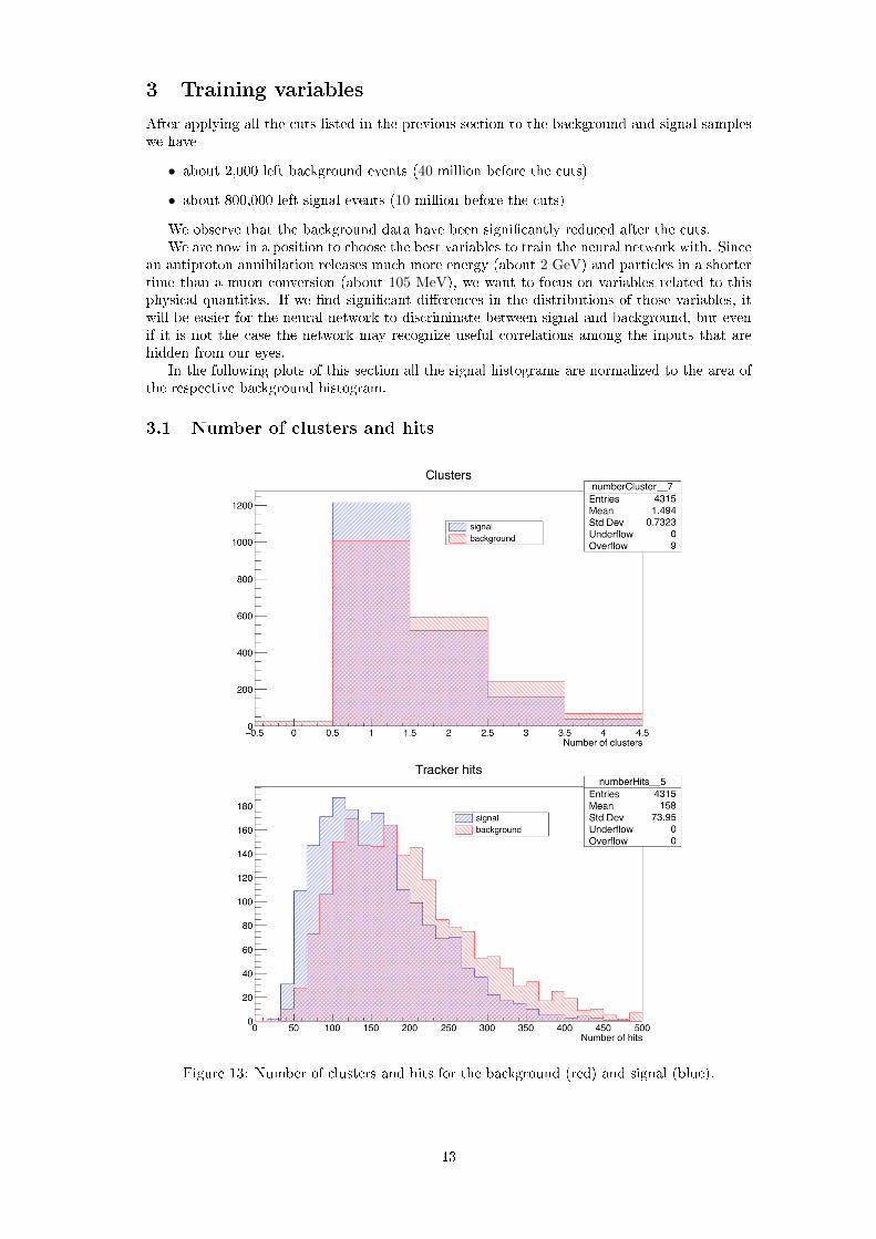
After applying all the cuts listed in the previous section to the background and signal sampleswe have

• about 2,000 left background events (40 million before the cuts)

• about 800,000 left signal events (10 million before the cuts)

We observe that the background data have been signi�cantly reduced after the cuts.We are now in a position to choose the best variables to train the neural network with. Since

an antiproton annihilation releases much more energy (about 2 GeV) and particles in a shortertime than a muon conversion (about 105 MeV), we want to focus on variables related to thisphysical quantities. If we �nd signi�cant di�erences in the distributions of those variables, itwill be easier for the neural network to discriminate between signal and background, but evenif it is not the case the network may recognize useful correlations among the inputs that arehidden from our eyes.

In the following plots of this section all the signal histograms are normalized to the area ofthe respective background histogram.

3.1 Number of clusters and hits

Figure 13: Number of clusters and hits for the background (red) and signal (blue).

13

Since more particles may be released in an antiproton annihilation, we want to check if moreclusters in the calorimeter and hits in the tracker arise compared to the signal. Their numberis shown in �gure 13: the excess in the background case cannot be only a statistical �uctuationand as we expected an antiproton annihilation has on average more clusters and hits than asignal event.

3.2 Clusters and hits time

In an antiproton annihilation many particles are produced in a short time: we may expect that,in the background events, clusters and hits related to the electron track arise earlier than in thesignal ones. Therefore we want to have a look at their average time distribution, which is shownin �gure 14: what we observe is that the background distribution of the cluster time has a peakjust some nanoseconds earlier than the signal distribution, as we could expect, whereas in thehits time distribution we can't see many di�erences. Despite it, we will keep both variablesin our training because there may be some correlations between them that we are not able torecognize.

Figure 14: Average time of the clusters and hits related to the track.

3.3 Clusters and hits energy

As we have already said, we expect to �nd more energy in an antiproton annihilation ratherthan in a signal event. The total energy distributions for the clusters and hits is shown in �gure15 and we observe two interesting features of them:

• The energy is generally higher for the background distributions;

14

Figure 15: Total energy of the clusters and hits related to the track. Note the long tail at highenergies in the background distributions.

• In the background case, the clusters and hits energy distributions show a long tail forhigh energies which is not shown in the signal case.

Both features are very interesting for our purpose and we can expect the energy variables tohave a high discriminating power in the neural network.

3.4 Highest cluster energy

Since the background events release more energy, we may expect to �nd more energetic particlesfrom them. We then want to �nd the highest cluster energy not related to the electron track forboth the signal and background. This distribution is shown in �gure 16 and we can recognizea long tail at high energy only in the background case. Since the di�erences for the signal andbackground distributions are clear, we may expect this variable to be very important in theneural network's training.

3.5 Clusters center of energy

The last variable we want to deal with is the square of the weighted average of the clustersdistances to the electron cluster, where the weighting factor is the energy of the clusters itself:

r2CoE =

∑i r

2iEi∑iEi

15

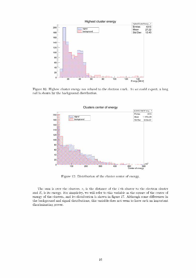
Figure 16: Highest cluster energy not related to the electron track. As we could expect, a longtail is shown by the background distribution.

Figure 17: Distribution of the cluster center of energy.

The sum is over the clusters, ri is the distance of the i-th cluster to the electron clusterand Ei is its energy. For simplicity, we will refer to this variable as the square of the center ofenergy of the clusters, and its distribution is shown in �gure 17. Although some di�erences inthe background and signal distributions, this variable does not seem to have such an importantdiscriminating power.

16

4 Neural network training

After we have decided the variables to deal with, we are able to use them to build the neuralnetwork. The neural network training will be developed in the ROOT environment of Mul-tivariate Analysis, which provides di�erent training methods. As we have already mentionedin section 1.4, in our work we will use three of them: the Boosted Decision Tree (BDT), theSupport Vector Machine (SVM) and the MultiLayer Perceptron (MLP). Each of these trainingmethods has di�erent features as we can read from �gure 6, so we may expect that the neuralnetwork shows di�erent behaviors depending on the chosen method.

The results of the neural network training are analyzed in the following subsections.

4.1 Output distributions

The aim of a neural network is to produce one or more outputs from the inputs provided, whichare then used to perform pattern recognition of the input data. More speci�cally, like in our case,the outputs can be used to discriminate between two kinds of events: signal and background.These outputs, being the �nal products of a neural network, are therefore extremely importantand can provide us with information about the network, like its behavior, its discriminatingpower, the overtraining and so on.

The output distributions for our three di�erent training methods are shown in �gure 18.They show at least two relevant aspects which are import to point out:

• Regarding the BDT, we can see that the background outputs for the training sample (redpoints) and the test sample (red histogram) do not overlap very well: it is a clear hintof overtraining (BDT is much sensitive to it, as we can realize from �gure 6). The sameproblem is not shown in the signal outputs, whose training and test samples overlap: thedi�erent response of the network to the signal and background events let us suppose thatthe problem may arise because of too few data in the background case.

• A look at the SVM output distributions shows that overtraining is not present in thiscase, but we have another problem: the signal and background distributions overlapalmost everywhere, meaning that the SVM is unable to discriminate between signal andbackground. For this reason we cannot expect a good discriminating power of our neuralnetwork if SVM is chosen to train it.

MLP instead does not show many problems, even if more events would probably have beenuseful.

4.2 Cut e�ciencies

Once we have the output distributions, we can choose an output cut value and reject all thoseevents whose output is less then the chosen value. By doing it we want to get rid of as muchbackground as possible while keeping an acceptable amount of signal events.

For example, having a look at the MLP output distributions in �gure 18, if we apply a cutat 0.2 and reject all the lower outputs, we can eliminate a signi�cant part of background anda small part of signal; but we can also decide to apply the cut at a higher value, let's say 0.4,which let us get rid of more background events but also of a larger amount of signal ones. Wetherefore want to optimize the cut value.

Figure 19 shows the signal and background e�ciency as a function of the cut value appliedon the output distributions for the three training methods. It also shows, in the green curve,the ratio S/

√S +B, where S is the number of signal events above the cut value and B the

number of background ones. Every green curve has a maximum for a certain output value, andthat value can be chosen as the optimal cut value.

If we neglect BDT, which is overtrained, we can say that:

• About SVM, the background and signal e�ciency curve are both above 90% for most ofthe output values, showing a sharp vertical fall around almost the same value. This iswhat we could expect after the considerations in section 4.1, and con�rms that SVM isnot so good at discriminating between signal and background.

17

Figure 18: Output distributions for the training methods adopted in this work: BDT (�rstplot), SVM (second plot) and MLP (third plot). In these plots, the points represent thetraining sample whereas the histograms refer to the test sample. In both cases, the red color isused for the background samples and the blue for the signal ones.

18

Figure 19: Signal (blue) and background (red) e�ciency as a function of the cut value for thethree training methods. The maximum of the green curve (the ratio S/

√S +B) can be used

to choose the optimal cut value.

19

• About MLP, we can see that the background e�ciency decreases earlier than the signale�ciency: we get rid of a reasonable part of the background yet at low output values,whereas the signal begins to decrease only after a higher value. This is what we wantfrom a good neural network: a clear separation between signal and background.

4.3 Background rejection and signal e�ciency

In the plots in �gure 19 one value of background and signal e�ciency is related to each out-put value: we can therefore construct the background rejection versus signal e�ciency curves,plotted in �gure 20, where each color refers to a di�erent training method. The backgroundrejection is de�ned as 1 − background e�ciency. From a good neural network we expect thesecurves to approach as much as possible the right upper corner, where we will be ideally able toreject the whole background and keep all the signal.

We can realize from �gure 20 that, whereas SVM has not performed a good job as wehad already expected, MLP has achieved a satisfying compromise, being able to reject (forexample) 80% of background while keeping 60% of signal. The same is true for BDT, but sincethis method has been overtrained, its results are not trustworthy.

Even if these values are not excellent (neural networks can perform even a better job), wecan be satis�ed if we consider the low statistics in our data.

Figure 20: Background rejection versus signal e�ciency curves for each training method.

4.4 Importance of variables

ROOT also provides us with the importance of each variable in the training phase; in thissection we want to focus on MLP, which turned out to be the best training method.

The importance of the variables for MLP is shown in �gure 21; the histogram has 8 columns,one for each variable, and the higher the column, the more important the related variable is.The importance Ii of the i-th variable is computed as follows [9]:

Ii = x̄2i

nh∑j=1

w2ij j = 1, ..., nvar

where x̄i is the sample mean of the i-th variable, wij the weight between the input-layer neuroni and the hidden-layer neuron j, nh the number of neurons in the hidden layer and nvar thenumber of neurons in the input layer (i.e. the number of variables).

20

In this plot the variables have been ordered according to their importance, and we realizefrom it that the most discriminating variables are the ones related to the calorimeter. Inparticular, the number of clusters and the cluster total energy have the best discriminatingpower, as we could expect according to what we said in section 3.

This is true for MLP, but di�erent training methods could �nd better discriminating featuresin di�erent variables; a �rst analysis suggests that the tracker variables are the most useful inthe BDT case, but we would need more statistics to examine this aspect.

Figure 21: Importance of variables in the MLP training method.

21

5 conclusions

To summarize, in order to build a neural network capable of discriminating between a signaland a background event, we �rst simulated millions of conversion electrons (signal events) andantiproton annihilations (background events); then we got rid of the trivial background byapplying some speci�c cuts on our data; �nally, analyzing the features of both kinds of eventswe chose some variables to train our neural network with.

The results of the training were provided in section 1.4, and we may conclude by assertingthat two of the three training methods adopted in this work did not result to produce a goodjob: SVM because of its low discriminating power, BDT because overtraining occurred duringthe building process of the network. Nonetheless, MLP performed a good job, achieving asatisfying background rejection and keeping more than half of the signals.

Although good, the MLP's results cannot be de�ned excellent, and we would like to improveits performances. One way to do it is to increase the statistics of our samples (especially in thebackground case), by simulating more and more events: that would probably avoid overtrainig,as occurred in the BDT case, and would reduce the statistical �uctuations of the data, lettingthe training methods (in particular SVM) recognize the features of background and signaldistributions more easily.

A second attempt to improve the MLP's performances is to look for more discriminatingvariables to add to the neural network. Whatever these variables are, we expect them to referto the energy and time of the detectors' response.

Unfortunately, the time for the analysis was reduced by the large amount of time neededto run the simulations. We spent at least three weeks to obtain the samples used in this workbecause:

• The number of events simulated were huge (millions);

• Some jobs did not successfully end;

• The codes were a�ected by some bugs which had to be �xed: it happened that these bugswere found out only after the jobs were run, resulting in a waste of time.

Therefore we had no much time to improve the analysis in the ways we described above, butwe believe that larger samples and more training variables will turn out to produce betterperformances of our neural network.

22

References

[1] Fundamental Physics at the Intensity Frontier, 2012.

[2] R. J. Abrams et al. Mu2e Conceptual Design Report. 2012.

[3] N. Atanov et al. The calorimeter of the Mu2e experiment at Fermilab. JINST,12(01):C01061, 2017.

[4] L. Bartoszek et al. Mu2e Technical Design Report. 2014.

[5] Robert H. Bernstein and Peter S. Cooper. Charged Lepton Flavor Violation: An Experi-menter's Guide. Phys. Rept., 532:27�64, 2013.

[6] R. M. Carey et al. Proposal to search for µ−N → e−N with a single event sensitivitybelow 10−16. 2008.

[7] Andrzej Czarnecki, Xavier Garcia i Tormo, and William J. Marciano. Muon decay in orbit:spectrum of high-energy electrons. Phys. Rev., D84:013006, 2011.

[8] Andrei Gaponenko. The Mu2e Experiment: A New High-Sensitivity Muon to ElectronConversion Search at Fermilab. In Proceedings, 11th Conference on the Intersections ofParticle and Nuclear Physics (CIPANP 2012): St. Petersburg, Florida, USA, May 29-June2, 2012, 2012.

[9] Andreas Hoecker, Peter Speckmayer, Joerg Stelzer, Jan Therhaag, Eckhard von Toerne,and Helge Voss. TMVA: Toolkit for Multivariate Data Analysis. PoS, ACAT:040, 2007.

[10] Luca Morescalchi. The Mu2e Experiment at Fermilab. PoS, DIS2016:259, 2016.

23