antennas - amanogawaamanogawa.com/archive/docs/antennas1.pdfantennas are in general reciprocal...
TRANSCRIPT
Antennas
© Amanogawa, 2006 – Digital Maestro Series 1
Antennas
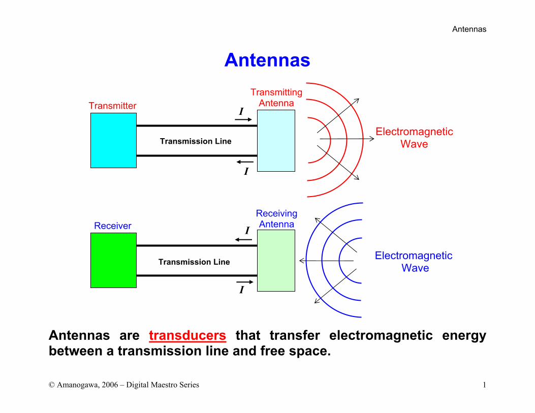
Antennas are transducers that transfer electromagnetic energy between a transmission line and free space.
Transmitting Antenna
I
I
Transmitter
Transmission Line Electromagnetic
Wave
Receiving Antenna
I
IReceiver
Transmission Line ElectromagneticWave
Antennas
© Amanogawa, 2006 – Digital Maestro Series 2
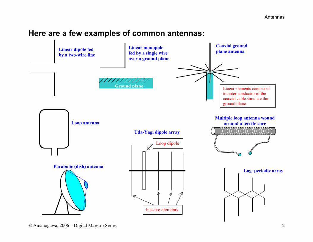
Here are a few examples of common antennas:
Linear dipole fed by a two-wire line
Ground plane
Linear monopole fed by a single wire over a ground plane
Coaxial ground plane antenna
Parabolic (dish) antenna
Linear elements connected to outer conductor of the coaxial cable simulate the ground plane
Uda-Yagi dipole array
Passive elements
Loop dipole
Log−periodic array
Loop antenna Multiple loop antenna wound
around a ferrite core
Antennas
© Amanogawa, 2006 – Digital Maestro Series 3
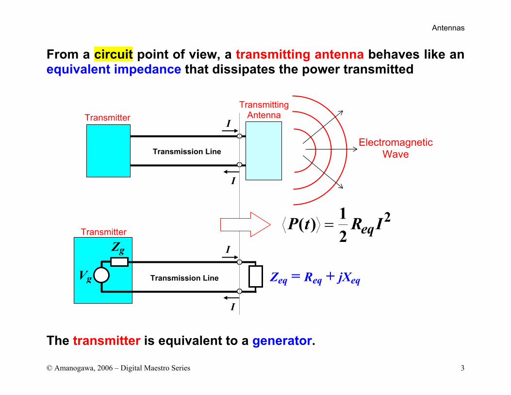
From a circuit point of view, a transmitting antenna behaves like an equivalent impedance that dissipates the power transmitted
The transmitter is equivalent to a generator.
I
I
Transmitter
Transmission Line
Transmitting Antenna
I
I
Transmitter
Transmission Line Electromagnetic
Wave
Zeq = Req + jXeq
P t R Ieq( ) =12
2
Vg
Zg
Antennas
© Amanogawa, 2006 – Digital Maestro Series 4
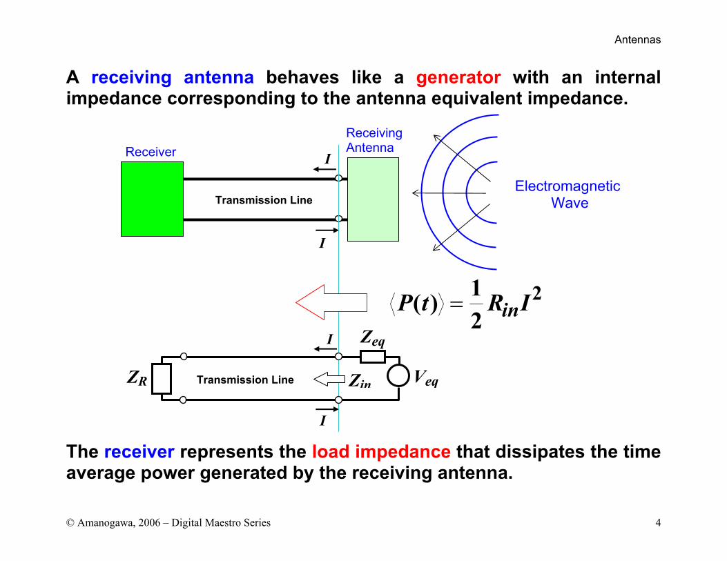
A receiving antenna behaves like a generator with an internal impedance corresponding to the antenna equivalent impedance.
The receiver represents the load impedance that dissipates the time average power generated by the receiving antenna.
I
I
Transmission Line
Receiving Antenna
I
I
Receiver
Transmission Line
P t R Iin( ) =12
2
Veq
Zeq
ElectromagneticWave
ZinZR
Antennas
© Amanogawa, 2006 – Digital Maestro Series 5
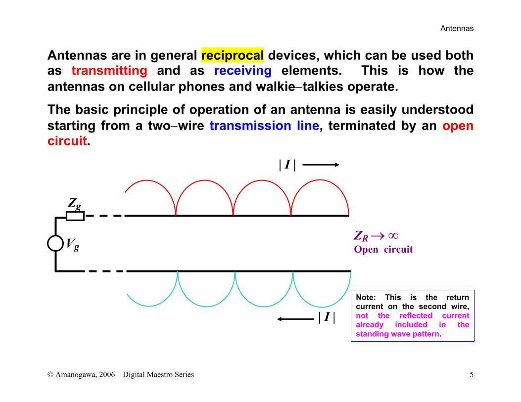
Antennas are in general reciprocal devices, which can be used both as transmitting and as receiving elements. This is how the antennas on cellular phones and walkie−talkies operate.
The basic principle of operation of an antenna is easily understood starting from a two−wire transmission line, terminated by an open circuit.
Vg
Zg
| I |
| I |Note: This is the return current on the second wire, not the reflected current already included in the standing wave pattern.
ZR → ∞ Open circuit
Antennas
© Amanogawa, 2006 – Digital Maestro Series 6
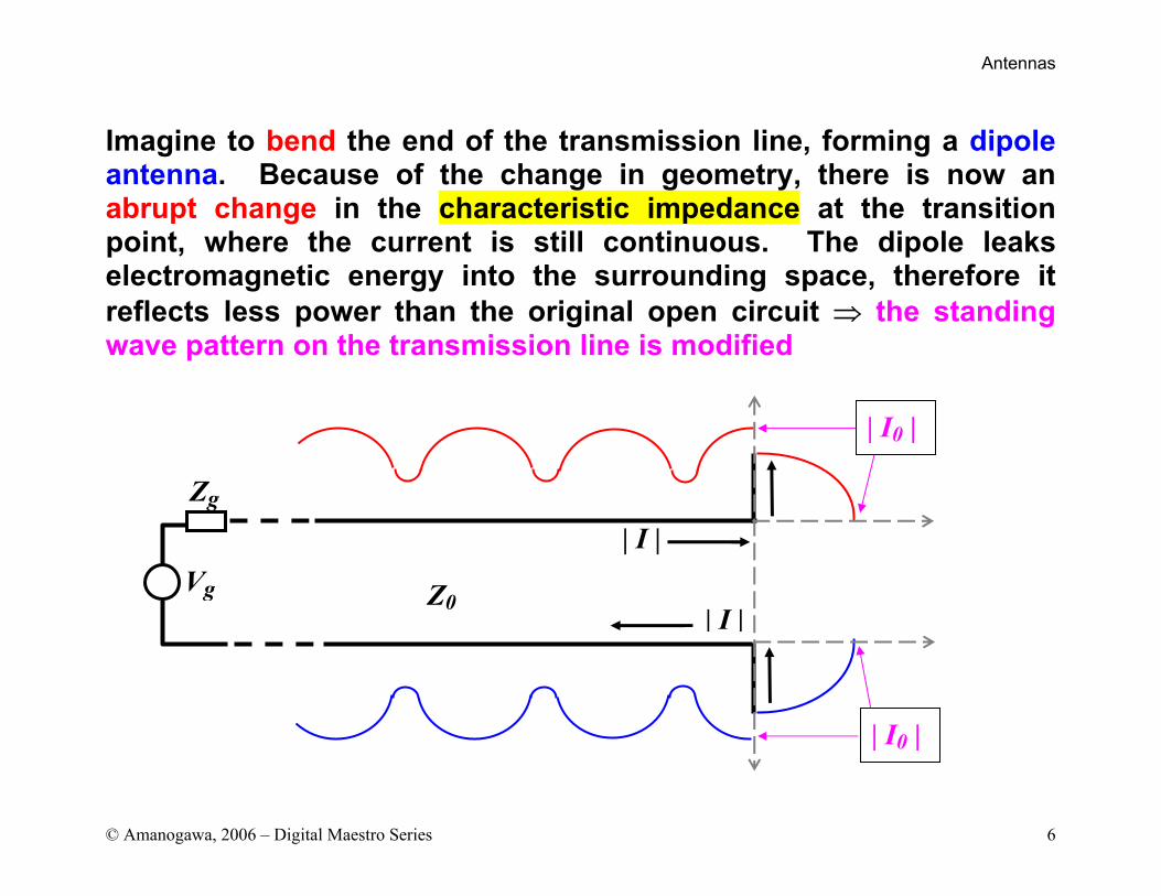
Imagine to bend the end of the transmission line, forming a dipole antenna. Because of the change in geometry, there is now an abrupt change in the characteristic impedance at the transition point, where the current is still continuous. The dipole leaks electromagnetic energy into the surrounding space, therefore it reflects less power than the original open circuit ⇒ the standing wave pattern on the transmission line is modified
Z0Vg
Zg
| I |
| I |
| I0 |
| I0 |
Antennas
© Amanogawa, 2006 – Digital Maestro Series 7
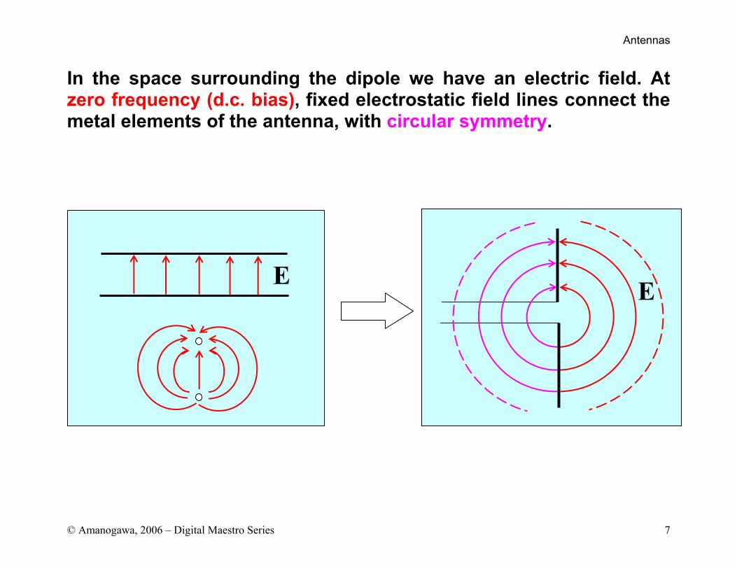
In the space surrounding the dipole we have an electric field. At zero frequency (d.c. bias), fixed electrostatic field lines connect the metal elements of the antenna, with circular symmetry.
E E
Antennas
© Amanogawa, 2006 – Digital Maestro Series 8
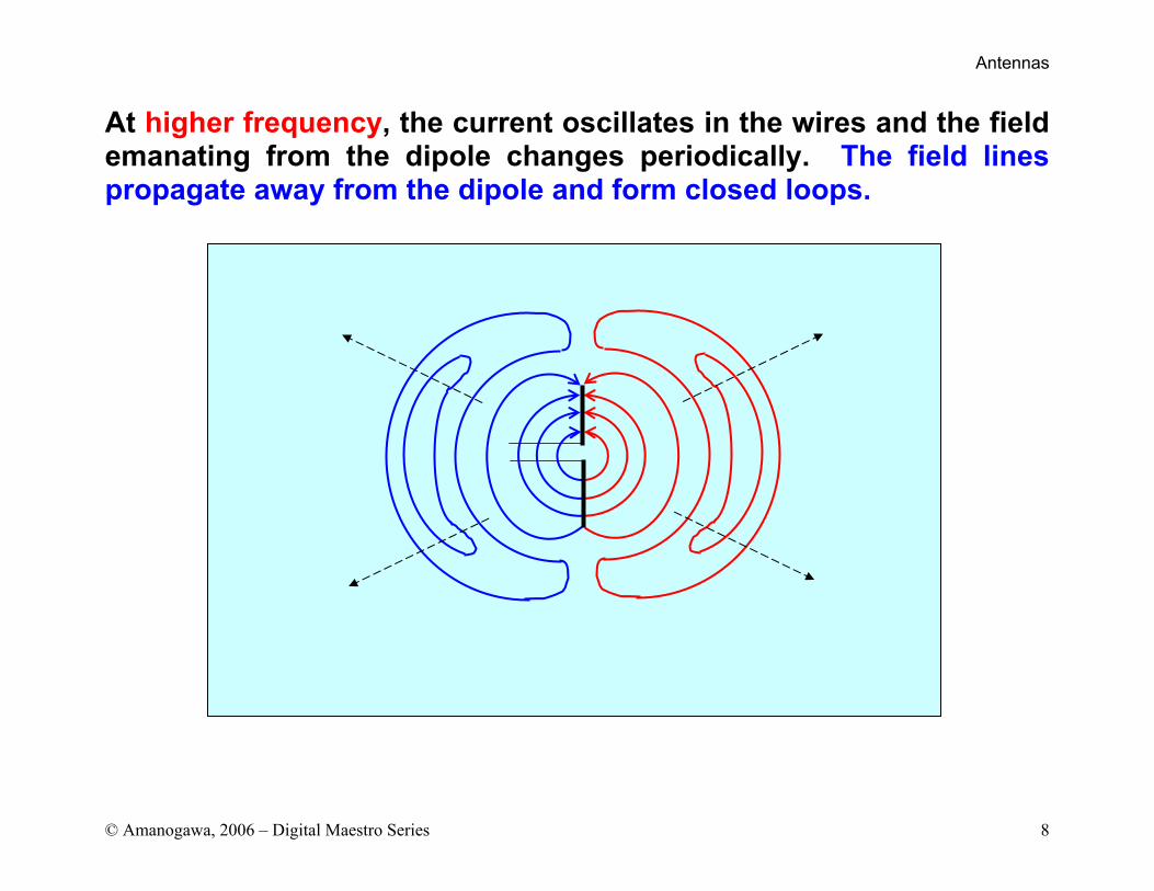
At higher frequency, the current oscillates in the wires and the field emanating from the dipole changes periodically. The field lines propagate away from the dipole and form closed loops.
Antennas
© Amanogawa, 2006 – Digital Maestro Series 9
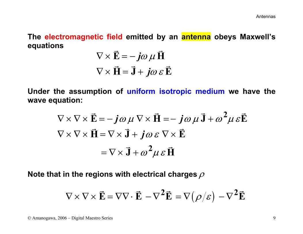
The electromagnetic field emitted by an antenna obeys Maxwell’s equations
Under the assumption of uniform isotropic medium we have the wave equation:
Note that in the regions with electrical charges ρ
jj
E HH J E
ω µω ε
∇ × = −
∇ × = +
2
2
E H J EH J E
J H
j jj
ω µ ω µ ω µ εω ε
ω µ ε
∇ × ∇ × = − ∇ × =− +
∇ × ∇ × = ∇ × + ∇ ×
= ∇ × +
( )2 2E E E Eρ ε∇ × ∇ × = ∇∇ ⋅ − ∇ = ∇ − ∇
Antennas
© Amanogawa, 2006 – Digital Maestro Series 10
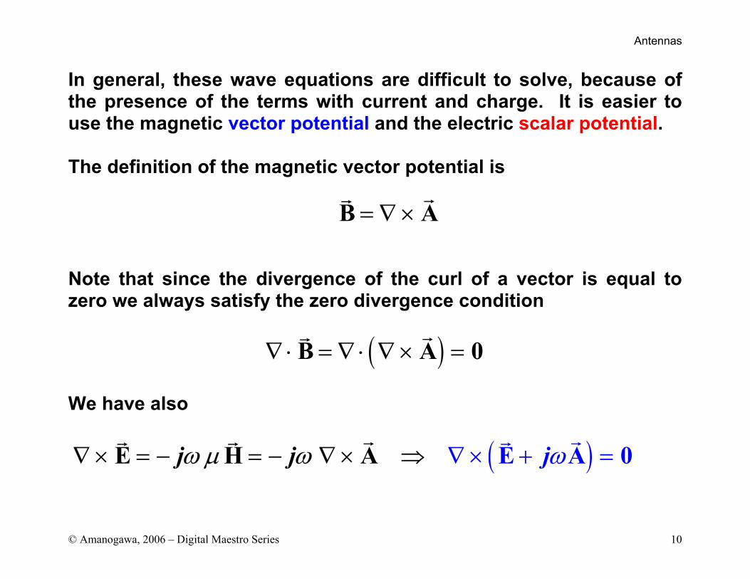
In general, these wave equations are difficult to solve, because of the presence of the terms with current and charge. It is easier to use the magnetic vector potential and the electric scalar potential. The definition of the magnetic vector potential is
Note that since the divergence of the curl of a vector is equal to zero we always satisfy the zero divergence condition
We have also
B A= ∇ ×
( )B A 0∇ ⋅ = ∇ ⋅ ∇ × =
( )j jj E AE H A 0ωω µ ω∇ × = − = − ∇ × × =⇒ ∇ +
Antennas
© Amanogawa, 2006 – Digital Maestro Series 11
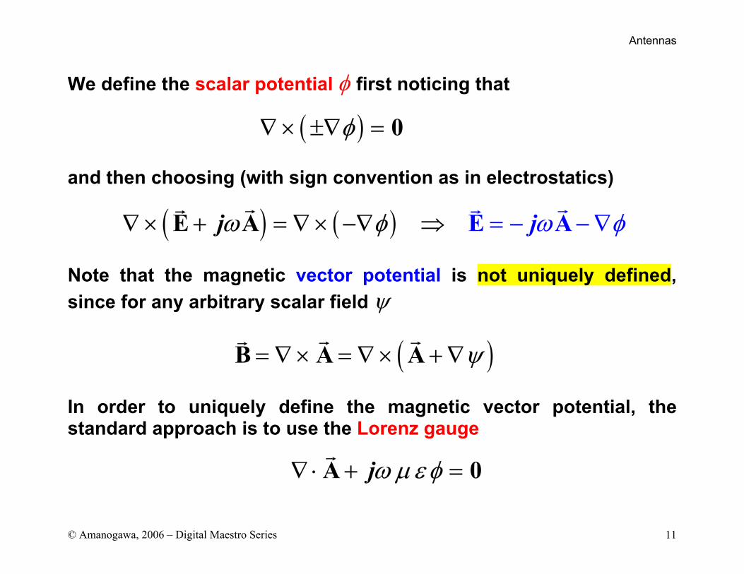
We define the scalar potential φ first noticing that
and then choosing (with sign convention as in electrostatics)
Note that the magnetic vector potential is not uniquely defined, since for any arbitrary scalar field ψ
In order to uniquely define the magnetic vector potential, the standard approach is to use the Lorenz gauge
( ) 0φ∇ × ±∇ =
( ) ( )E A E Ajj ωω φ φ∇ × + = ∇ × −∇ − − ∇⇒ =
( )B A A ψ= ∇ × = ∇ × + ∇
jA 0ω µε φ∇ ⋅ + =
Antennas
© Amanogawa, 2006 – Digital Maestro Series 12
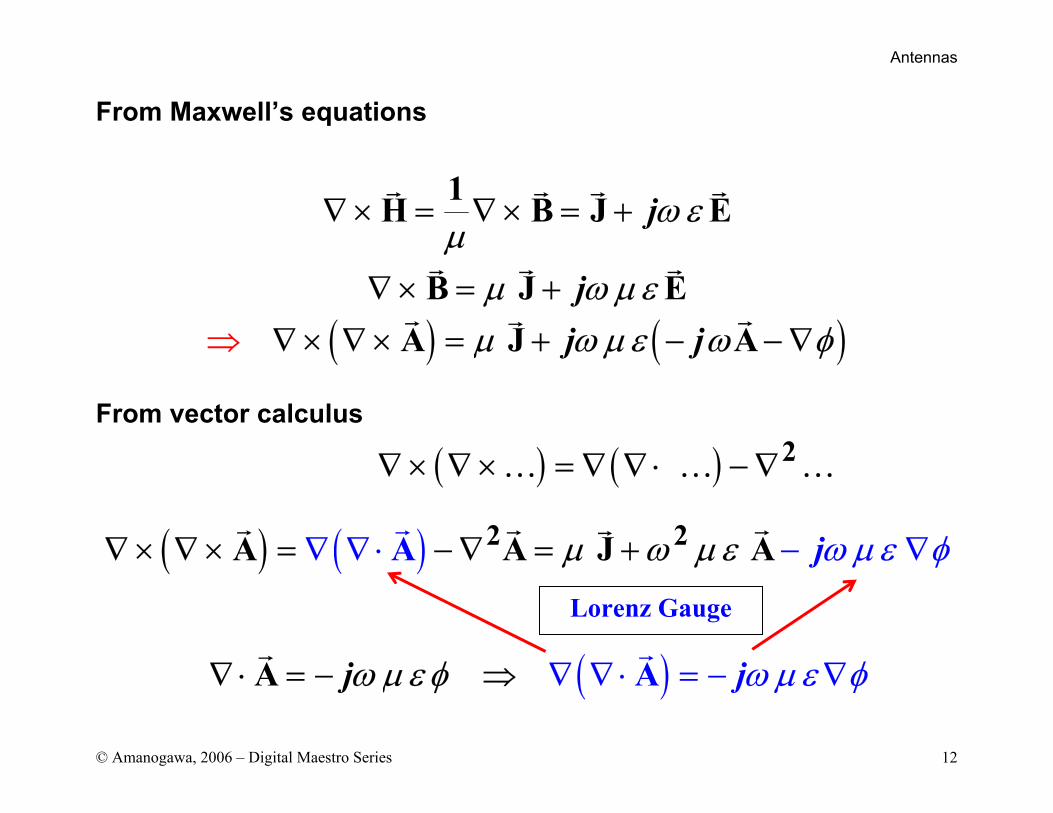
From Maxwell’s equations
From vector calculus
( ) ( )
j
jj j
1H B J E
B J EA J A
ω εµ
µ ω µ εµ ω µ ε ω φ
∇ × = ∇ × = +
∇ × = +∇ × ∇ × = + − − ∇⇒
( ) ( ) j2 2AA A J A ω µ ε φµ ω µ ε∇ × ∇ × = − ∇ =∇ ∇ ⋅ − ∇+
( )j jAA ω ω µ φµ ε φ ε∇∇ ⋅ = − ⇒ ∇⋅ = − ∇
Lorenz Gauge
( ) ( ) 2∇ × ∇ × = ∇ ∇ ⋅ − ∇… … …
Antennas
© Amanogawa, 2006 – Digital Maestro Series 13
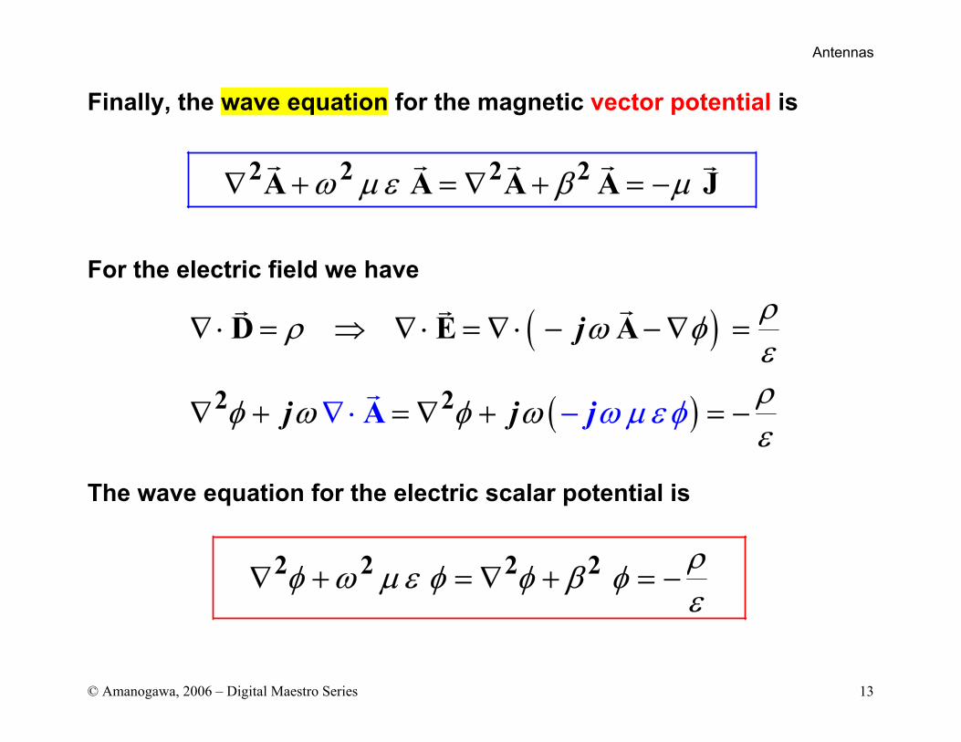
Finally, the wave equation for the magnetic vector potential is For the electric field we have
The wave equation for the electric scalar potential is
2 2 2 2A A A A Jω µε β µ∇ + = ∇ + = −
( )
( )2 2
D E
A
Aj
j j jω µε φ
ρρ ω φερφ ω φ ωε
∇ ⋅ = ⇒ ∇⋅ = ∇ ⋅ − − ∇ =
∇ + = ∇ +∇ ⋅ = −−
2 2 2 2 ρφ ω µ ε φ φ β φε
∇ + = ∇ + = −
Antennas
© Amanogawa, 2006 – Digital Maestro Series 14
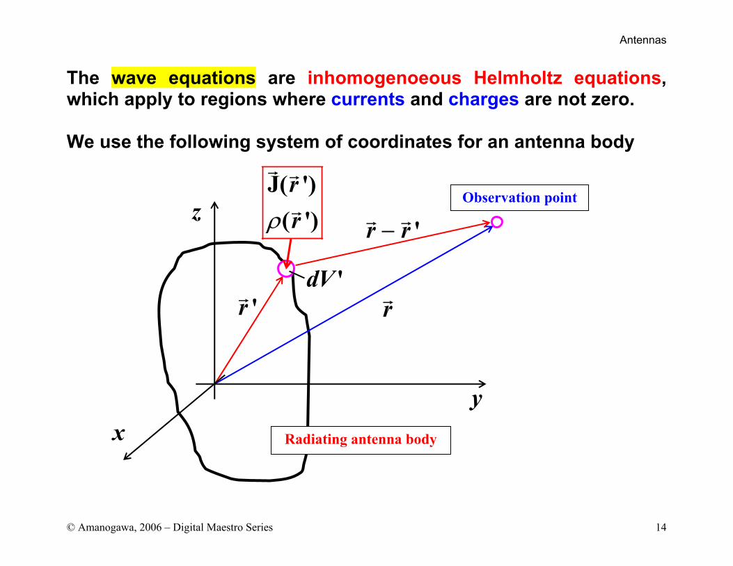
The wave equations are inhomogenoeous Helmholtz equations, which apply to regions where currents and charges are not zero. We use the following system of coordinates for an antenna body
z
xy
rr '
r r '−
Radiating antenna body
Observation pointrr
J( ')( ')ρ
dV '
Antennas
© Amanogawa, 2006 – Digital Maestro Series 15
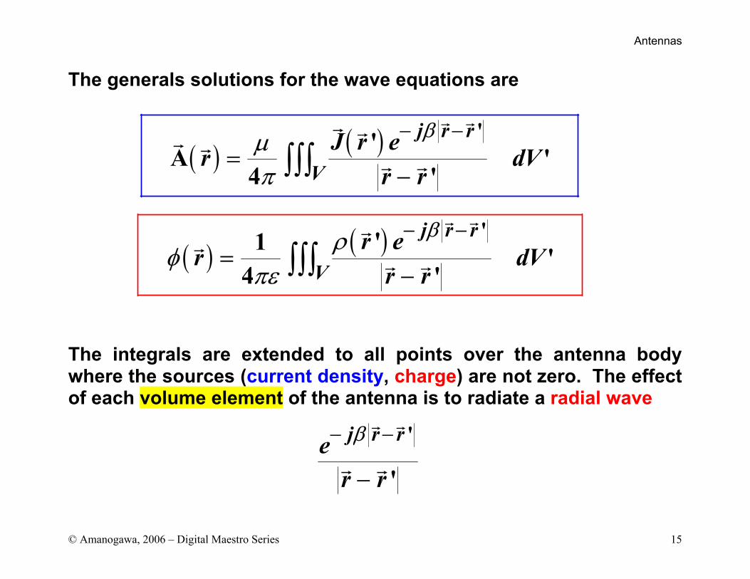
The generals solutions for the wave equations are
The integrals are extended to all points over the antenna body where the sources (current density, charge) are not zero. The effect of each volume element of the antenna is to radiate a radial wave
( ) ( ) j r r
VJ r er dV
r r
''A '
4 '
βµπ
− −=
−∫∫∫
( ) ( ) j r r
Vr er dV
r r
''1 '4 '
βρφ
πε
− −=
−∫∫∫
j r rer r
'
'
β− −
−
Antennas
© Amanogawa, 2006 – Digital Maestro Series 16
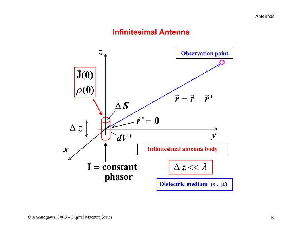
Infinitesimal Antenna
z
xy
r r r '= −
r ' 0=
Infinitesimal antenna body
Observation point
J(0)(0)ρ
dV '
S∆
z∆
I constant phasor= z λ∆ <<
Dielectric medium (ε , µ)
Antennas
© Amanogawa, 2006 – Digital Maestro Series 17
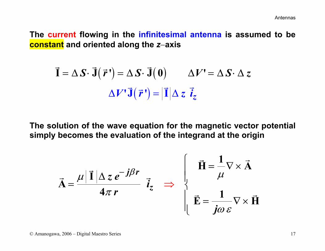
The current flowing in the infinitesimal antenna is assumed to be constant and oriented along the z−axis
The solution of the wave equation for the magnetic vector potential simply becomes the evaluation of the integrand at the origin
( ) ( )( ) z
S r S
V r z
V
i
S zI J ' J 0 '
'J ' I
= ∆ ⋅ = ∆ ⋅ ∆ =
∆ ∆
∆
=
∆ ⋅
1H AI
A4 1E H
j r
zz e
ir
j
β µµπ
ω ε
−⇒
= ∇ ×∆ = = ∇ ×
Antennas
© Amanogawa, 2006 – Digital Maestro Series 18
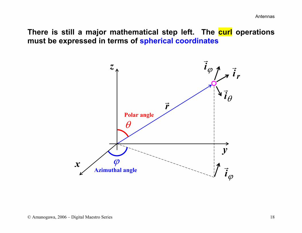
There is still a major mathematical step left. The curl operations must be expressed in terms of spherical coordinates
z
xy
r
θ
ϕiϕ
iϕ
iθ
ri
Azimuthal angle
Polar angle
Antennas
© Amanogawa, 2006 – Digital Maestro Series 19
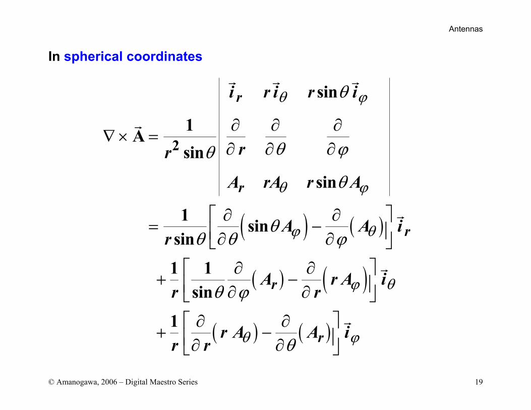
In spherical coordinates
( ) ( )
( ) ( )
( ) ( )
r
r
r
r
r
i r i r i
rr
A rA r A
A A ir
A r A ir r
r A A ir r
2
sin
1Asin
sin
1 sinsin
1 1sin
1
θ ϕ
θ ϕ
ϕ θ
ϕ θ
θ ϕ
θ
θ ϕθ
θ
θθ θ ϕ
θ ϕ
θ
∂ ∂ ∂∇ × =
∂ ∂ ∂
∂ ∂ = − ∂ ∂
∂ ∂ + − ∂ ∂
∂ ∂ + − ∂ ∂
Antennas
© Amanogawa, 2006 – Digital Maestro Series 20
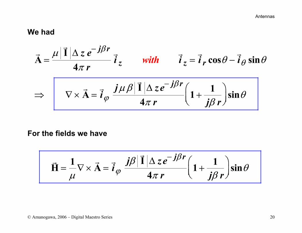
We had
For the fields we have
j r
z z r
j r
z ei i i i
r
j z ei
r r
ith
j
wI
A cos sin4
I 1A 1 sin4
β
θ
β
ϕ
µθ θ
π
µ βθ
π β
−
−
∆= = −
∆ ⇒ ∇ × = +
j rj z ei
r j rI1 1H A 1 sin
4
β
ϕβ
θµ π β
−∆ = ∇ × = +
Antennas
© Amanogawa, 2006 – Digital Maestro Series 21
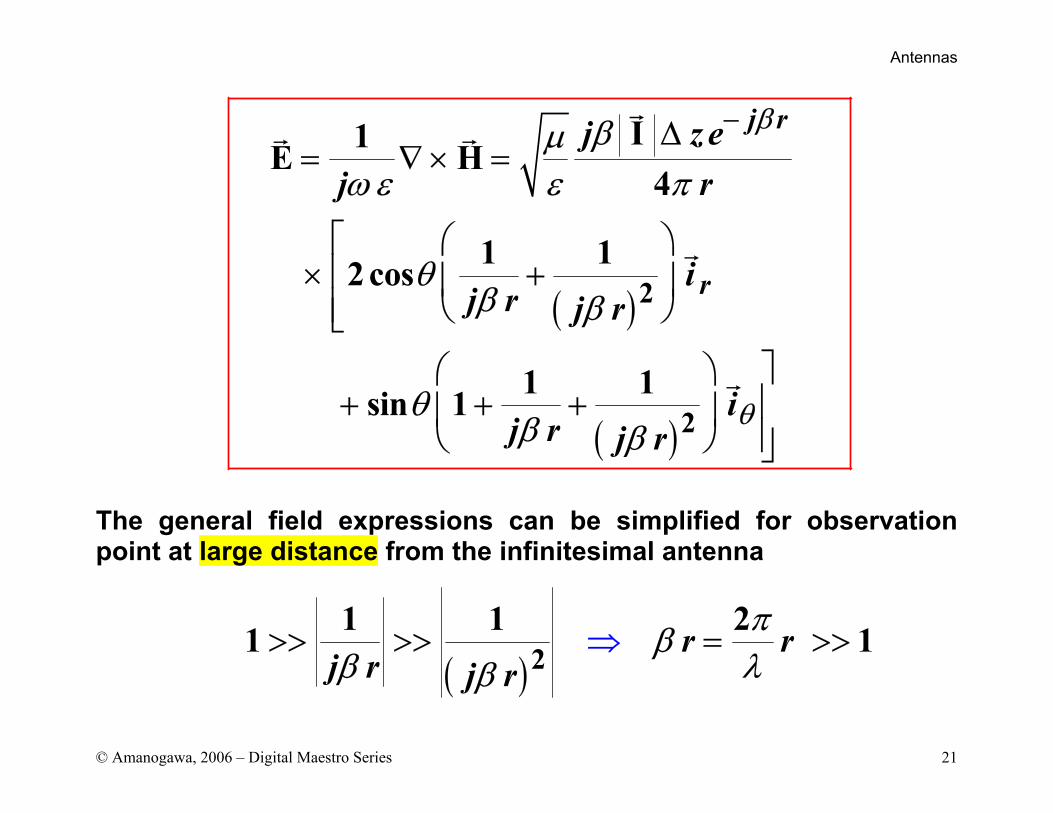
The general field expressions can be simplified for observation point at large distance from the infinitesimal antenna
( )
( )
j r
r
j z ej r
ij r j r
ij r j r
2
2
I1E H4
1 12 cos
1 1sin 1
β
θ
βµω ε ε π
θβ β
θβ β
−∆= ∇ × =
× +
+ + +
( )r r
j r j r 21 1 21 1πββ λβ
>> >> ⇒ = >>
Antennas
© Amanogawa, 2006 – Digital Maestro Series 22
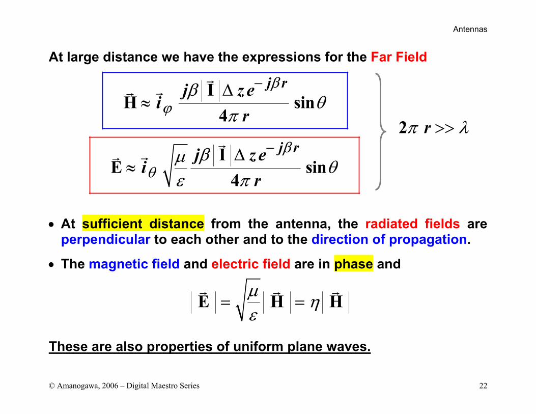
At large distance we have the expressions for the Far Field
• At sufficient distance from the antenna, the radiated fields are perpendicular to each other and to the direction of propagation.
• The magnetic field and electric field are in phase and
These are also properties of uniform plane waves.
E H Hµ ηε
= =
j rj z ei
rI
H sin4
β
ϕβ
θπ
−∆≈
j rj z ei
rI
E sin4
β
θβµ θ
ε π
−∆≈
r2π λ>>
Antennas
© Amanogawa, 2006 – Digital Maestro Series 23
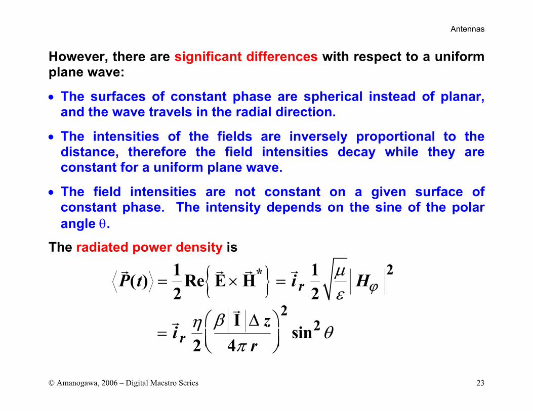
However, there are significant differences with respect to a uniform plane wave:
• The surfaces of constant phase are spherical instead of planar, and the wave travels in the radial direction.
• The intensities of the fields are inversely proportional to the distance, therefore the field intensities decay while they are constant for a uniform plane wave.
• The field intensities are not constant on a given surface of constant phase. The intensity depends on the sine of the polar angle θ.
The radiated power density is
2*
22
1 1( ) Re E H2 2
Isin
2 4
r
r
P t i H
zi
r
ϕµε
βη θπ
= × =
∆ =
Antennas
© Amanogawa, 2006 – Digital Maestro Series 24
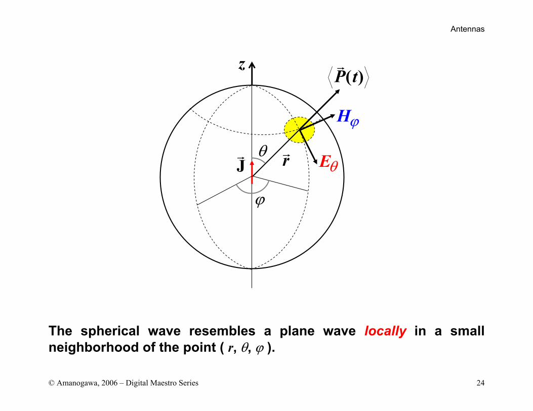
The spherical wave resembles a plane wave locally in a small neighborhood of the point ( r, θ, ϕ ).
z( )P t
Eθ
Hϕ
rθJ
ϕ
Antennas
© Amanogawa, 2006 – Digital Maestro Series 25
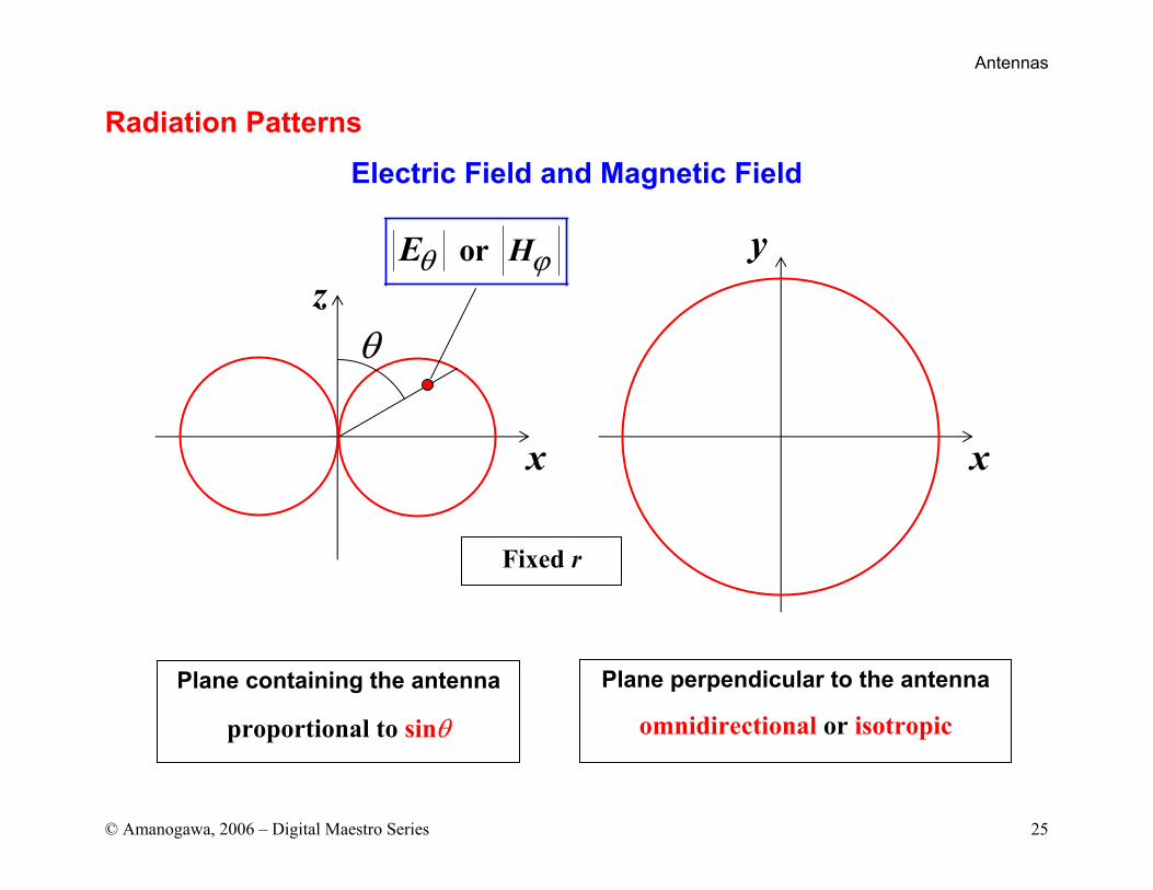
Radiation Patterns
Electric Field and Magnetic Field
z
x
or HEθ ϕ
θ
y
x
Plane containing the antenna
proportional to sinθ
Plane perpendicular to the antenna
omnidirectional or isotropic
Fixed r
Antennas
© Amanogawa, 2006 – Digital Maestro Series 26
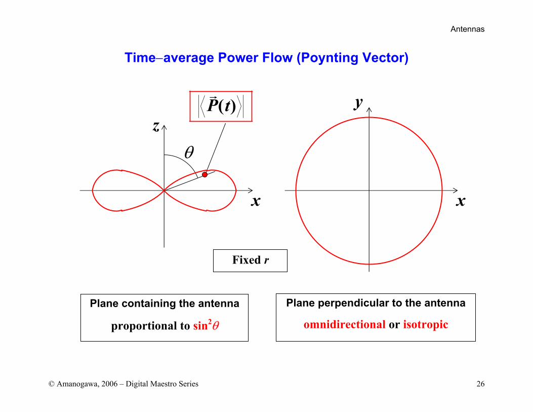
Time−average Power Flow (Poynting Vector)
z
x
( )P t
θ
Plane containing the antenna
proportional to sin2θ
Plane perpendicular to the antenna
omnidirectional or isotropic
y
x
Fixed r
Antennas
© Amanogawa, 2006 – Digital Maestro Series 27
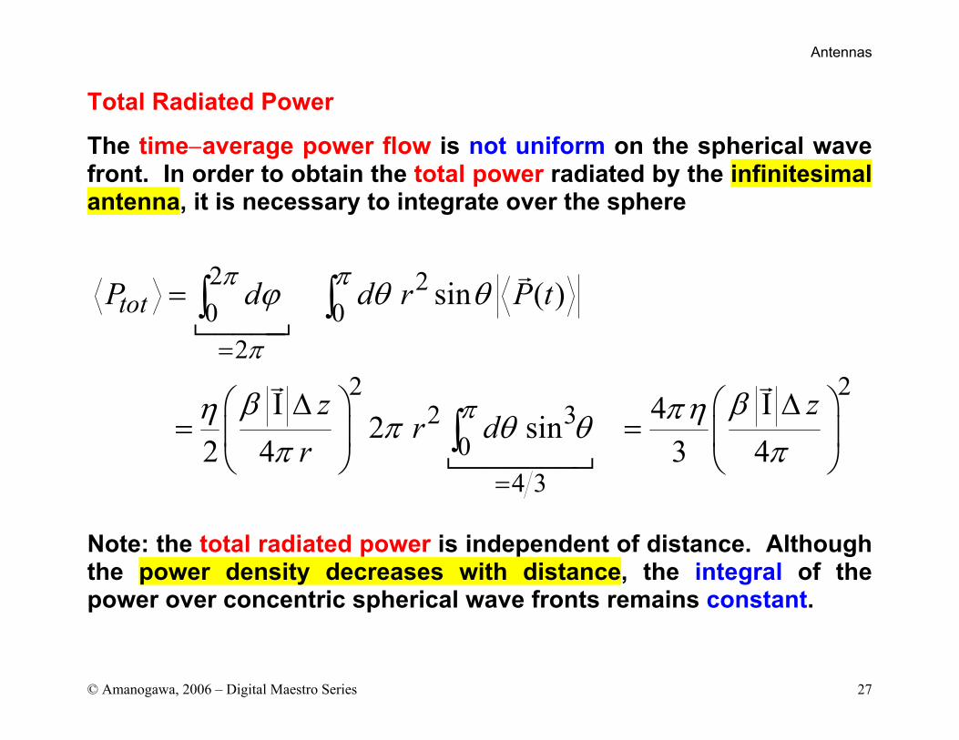
Total Radiated Power
The time−average power flow is not uniform on the spherical wave front. In order to obtain the total power radiated by the infinitesimal antenna, it is necessary to integrate over the sphere
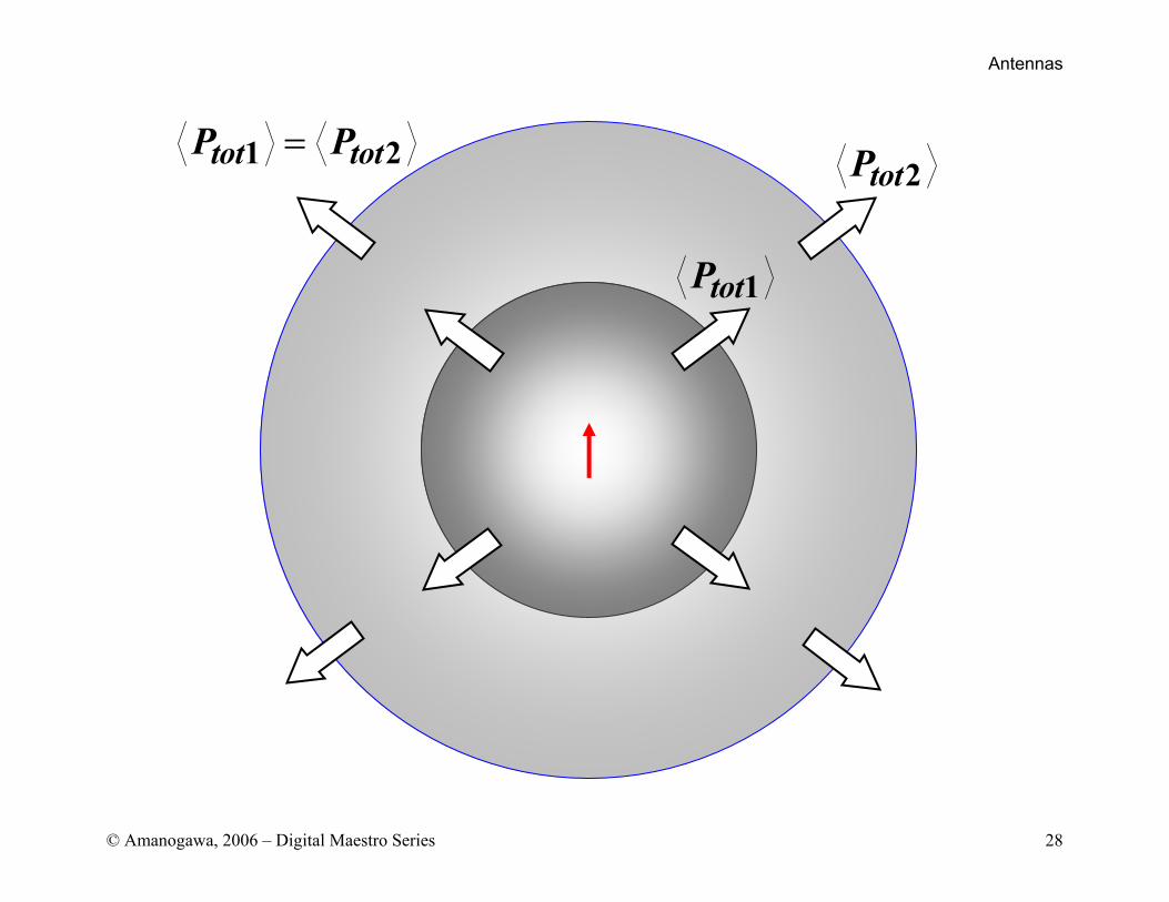
Note: the total radiated power is independent of distance. Although the power density decreases with distance, the integral of the power over concentric spherical wave fronts remains constant.
2 20 0
22 2
2 30
4 3
sin ( )
I I42 sin2 4 3 4
totP d d r P t
z zr d
r
π π
π
π
ϕ θ θ
β βη πηπ θ θπ π
=
=
=
∆ ∆= =
∫ ∫
∫
Antennas
© Amanogawa, 2006 – Digital Maestro Series 28
1 2tot totP P=
1totP
2totP
Antennas
© Amanogawa, 2006 – Digital Maestro Series 29
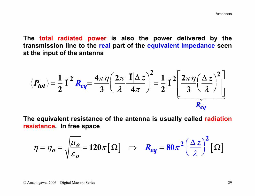
The total radiated power is also the power delivered by the transmission line to the real part of the equivalent impedance seen at the input of the antenna
The equivalent resistance of the antenna is usually called radiation resistance. In free space
2 22 2I1 4 2 1 2I I
2 3 4 2 3
eq
tot eq
R
z zP R πη π πηλ π λ
∆ ∆ = = =
[ ] [ ]2
2820 01oo
eqozR πµη π
λη
ε= =
∆
= Ω =
⇒ Ω
Antennas
© Amanogawa, 2006 – Digital Maestro Series 30
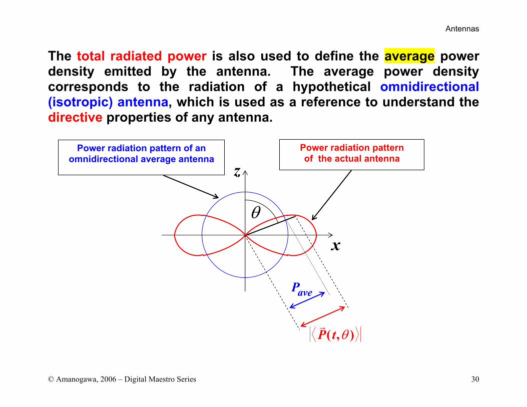
The total radiated power is also used to define the average power density emitted by the antenna. The average power density corresponds to the radiation of a hypothetical omnidirectional (isotropic) antenna, which is used as a reference to understand the directive properties of any antenna.
z
x
( , )P t θ
θ
aveP
Power radiation pattern of an omnidirectional average antenna
Power radiation pattern of the actual antenna
Antennas
© Amanogawa, 2006 – Digital Maestro Series 31
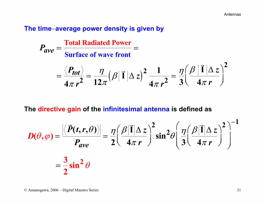
The time−average power density is given by
The directive gain of the infinitesimal antenna is defined as
( )
Surface of wave front2
22
Total Radiated Powe
2
r
I1I12 3 44 4
ave
tot
P
zP zrr r
βη ηβπ ππ π
= =
∆ = = ∆ =
12 22
2
( , , ) I Isi( , )
3 sin2
n2 4 3 4ave
P t r z zP r r
Dθ β βη ηθθ
θ
πϕ
π
− ∆ ∆ = =
=
Antennas
© Amanogawa, 2006 – Digital Maestro Series 32
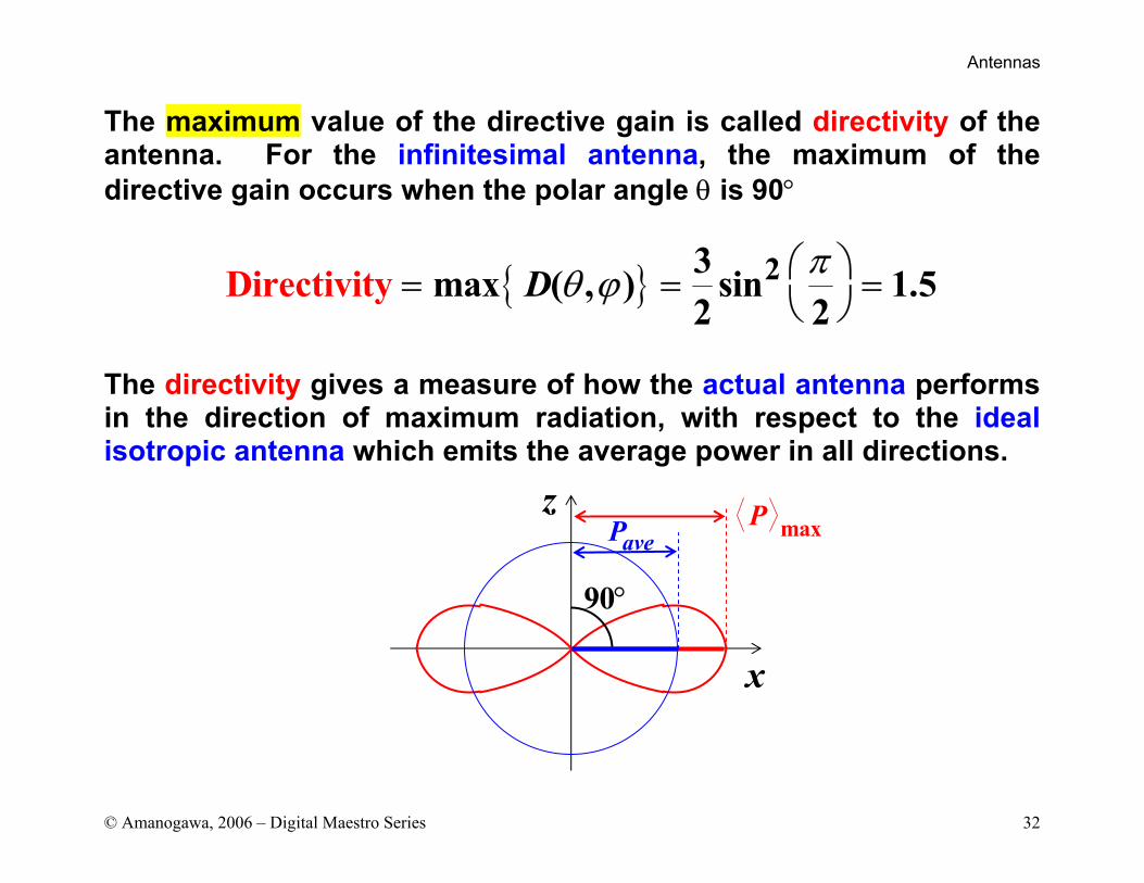
The maximum value of the directive gain is called directivity of the antenna. For the infinitesimal antenna, the maximum of the directive gain occurs when the polar angle θ is 90°
The directivity gives a measure of how the actual antenna performs in the direction of maximum radiation, with respect to the ideal isotropic antenna which emits the average power in all directions.
23max ( , ) sin 1Directivi .t2 2
y 5D πθ ϕ = = =
x
z
90°
aveP maxP
Antennas
© Amanogawa, 2006 – Digital Maestro Series 33
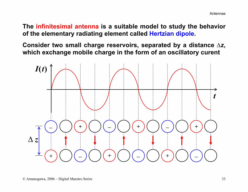
The infinitesimal antenna is a suitable model to study the behavior of the elementary radiating element called Hertzian dipole.
Consider two small charge reservoirs, separated by a distance ∆z, which exchange mobile charge in the form of an oscillatory curent
+
−
( )I t
t
z∆
+
−
+
−+
−
+
− +
−
Antennas
© Amanogawa, 2006 – Digital Maestro Series 34
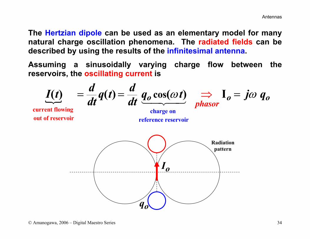
The Hertzian dipole can be used as an elementary model for many natural charge oscillation phenomena. The radiated fields can be described by using the results of the infinitesimal antenna.
Assuming a sinusoidally varying charge flow between the reservoirs, the oscillating current is
current flowing out of reser
charge on reference resevoir rvoir
cos( ) ( ) ( ) Iphaso
or
o od dI t q t q t j qdt dt ω ω= = =⇒
Radiation pattern
oq
oI
Antennas
© Amanogawa, 2006 – Digital Maestro Series 35
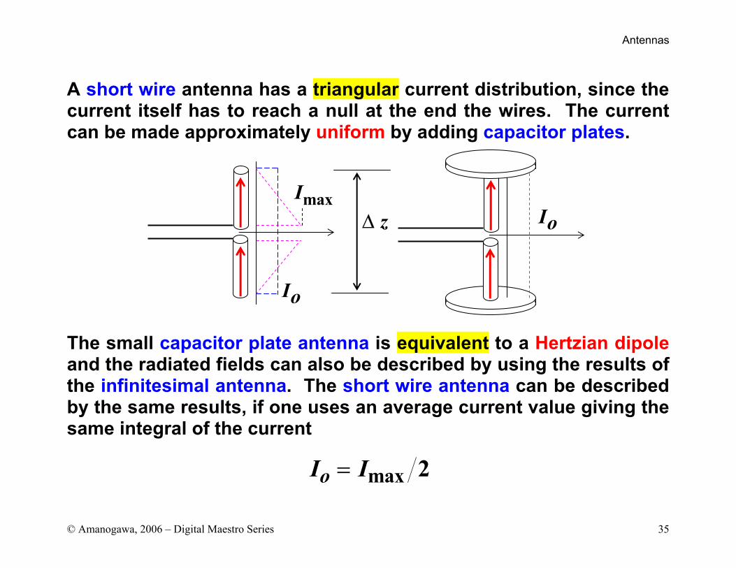
A short wire antenna has a triangular current distribution, since the current itself has to reach a null at the end the wires. The current can be made approximately uniform by adding capacitor plates.
The small capacitor plate antenna is equivalent to a Hertzian dipole and the radiated fields can also be described by using the results of the infinitesimal antenna. The short wire antenna can be described by the same results, if one uses an average current value giving the same integral of the current
max 2oI I=
ImaxIoz∆
Io
Antennas
© Amanogawa, 2006 – Digital Maestro Series 36
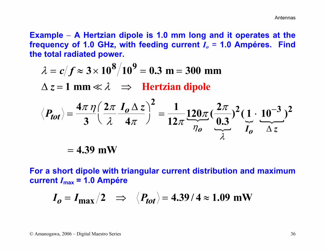
Example − A Hertzian dipole is 1.0 mm long and it operates at the frequency of 1.0 GHz, with feeding current Io = 1.0 Ampéres. Find the total radiated power.
For a short dipole with triangular current distribution and maximum current Imax = 1.0 Ampére
8 9
22 3 2
Hertzian dipole3 10 10 0.3 m 300 mm
1 mm
4 2 1 2120 ( ) ( 1 10 )3 4 12 0.3
4.39 mW
o o
otot
I z
c fz
I zPη
λ
λλ
π η π ππλ π π
−
∆
= ≈ × = =∆ = ⇒
∆ = = ⋅
=
max 2 4.39 / 4 1.09 mWo totI I P= ⇒ = ≈
Antennas
© Amanogawa, 2006 – Digital Maestro Series 37
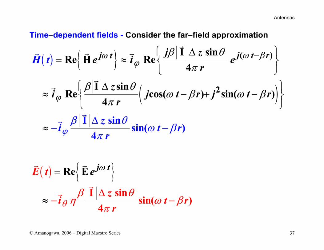
Time−dependent fields - Consider the far−field approximation
( )
( )
( )
( )
2
I sinRe H Re
4
I sinRe cos( ) sin
I sins
I sinsin(
in
( )4
Re
( )
4
4
E
)
j t rj t
j t
j ze i e
r
zi j t r j t
E t
H t
zi t r
r
t
r
e
r
r
zi
rθ
ω βωϕ
ϕ
ϕ
ω
β θπ
β
β θη ω
θω β ω
β θω
π
π
β
β
π
β
−∆ = ≈
∆
≈ − + −
≈
=
≈ − −
∆−
∆
−
Antennas
© Amanogawa, 2006 – Digital Maestro Series 38
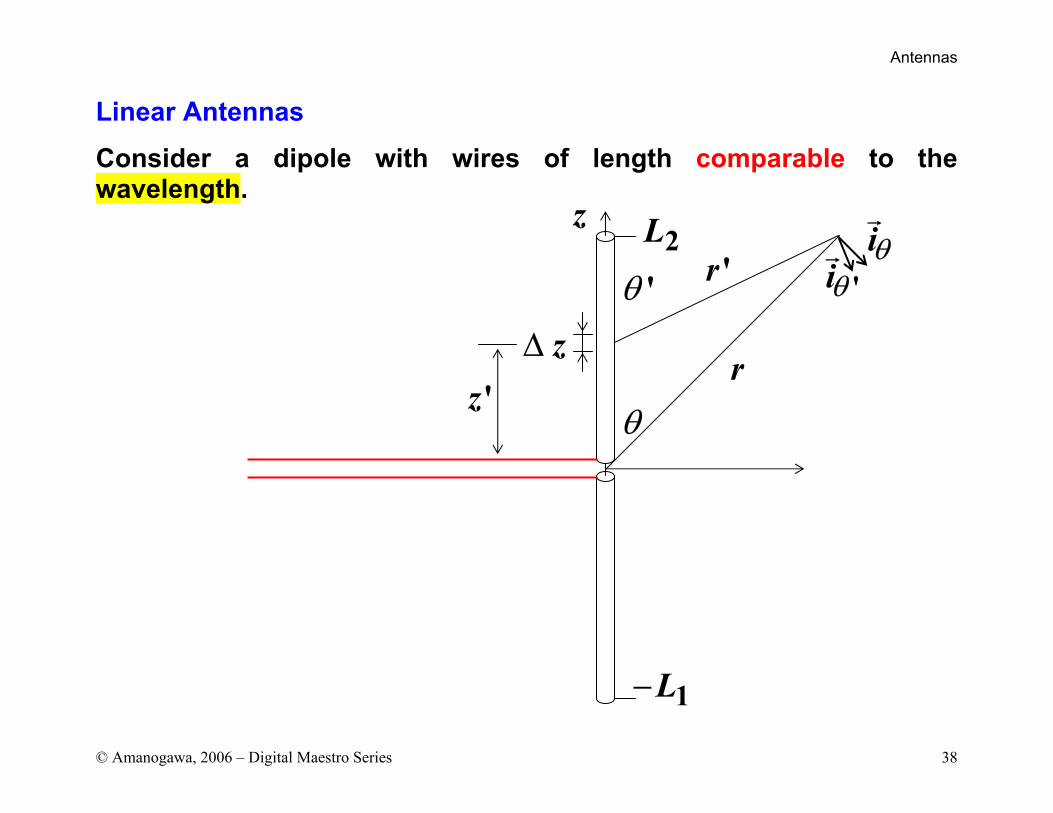
Linear Antennas
Consider a dipole with wires of length comparable to the wavelength.
z∆
'θ
θ
'r
r
'iθiθ
'z
z
1L−
2L
Antennas
© Amanogawa, 2006 – Digital Maestro Series 39
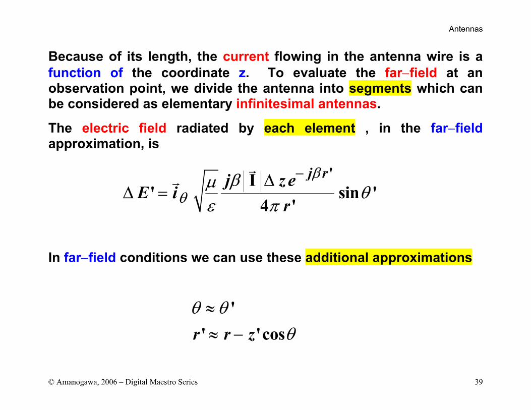
Because of its length, the current flowing in the antenna wire is a function of the coordinate z. To evaluate the far−field at an observation point, we divide the antenna into segments which can be considered as elementary infinitesimal antennas.
The electric field radiated by each element , in the far−field approximation, is
In far−field conditions we can use these additional approximations
'I' sin '
4 '
j rj z eE i
r
β
θβµ θ
ε π
−∆∆ =
r r z'
' 'cosθ θ
θ≈≈ −
Antennas
© Amanogawa, 2006 – Digital Maestro Series 40
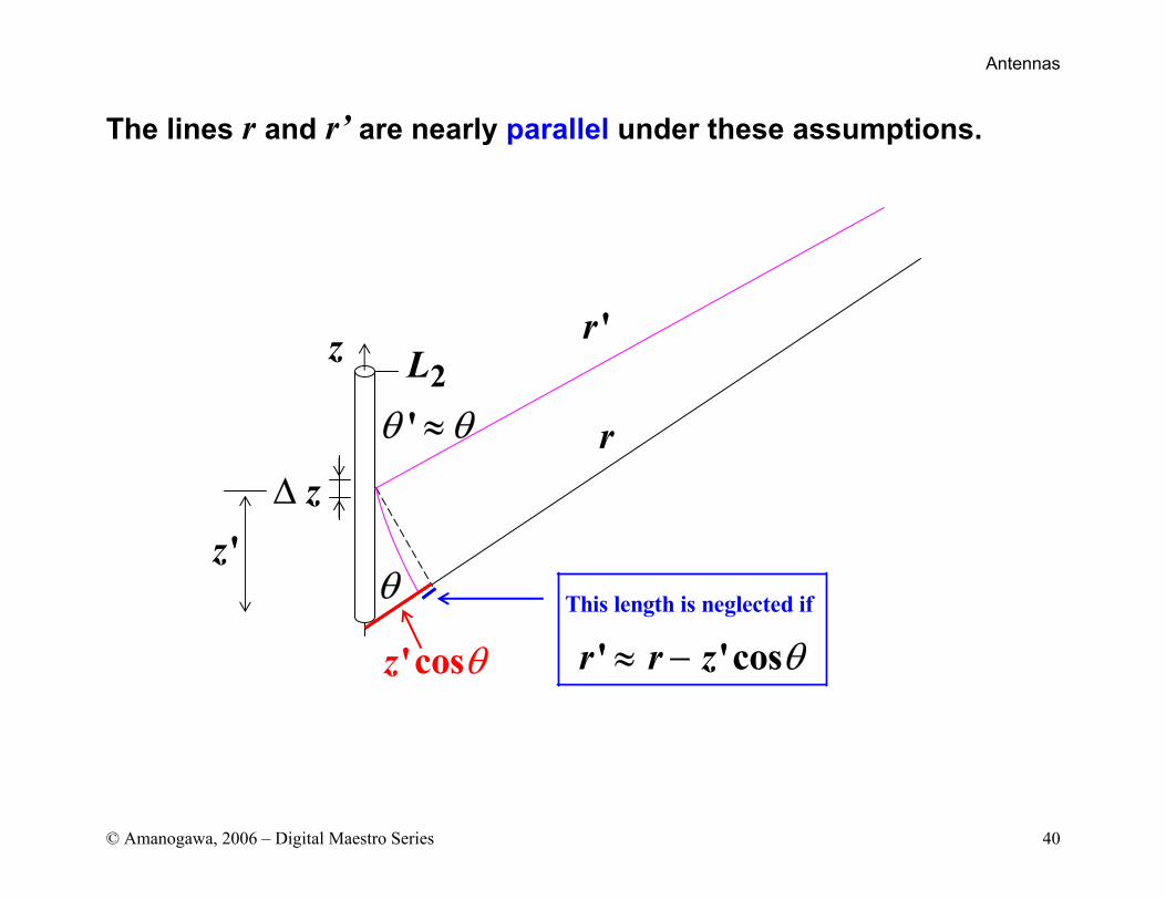
The lines r and r’ are nearly parallel under these assumptions.
z∆
'θ θ≈
θ
'r
r
'z
z2L
'cosz θThis length is neglected if
' 'cosr r z θ≈ −
Antennas
© Amanogawa, 2006 – Digital Maestro Series 41
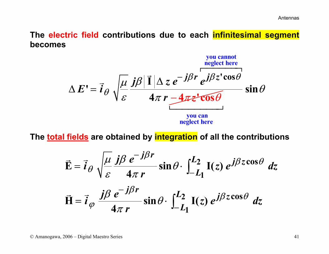
The electric field contributions due to each infinitesimal segment becomes
The total fields are obtained by integration of all the contributions
you cannotneglect here
'cos
4 'cosI
'4
j r j zj z e eE i
r z
β β θ
θβµ
ε π θπ
−∆∆ =
−
you can neglect here
sinθ
21
21
cos
cos
E sin I( )4
H sin I( )4
j r L j zL
j r L j zL
j ei z e dzr
j ei z e dzr
ββ θ
θ
ββ θ
ϕ
µ β θε π
β θπ
−
−
−
−
= ⋅
= ⋅
∫
∫
Antennas
© Amanogawa, 2006 – Digital Maestro Series 42
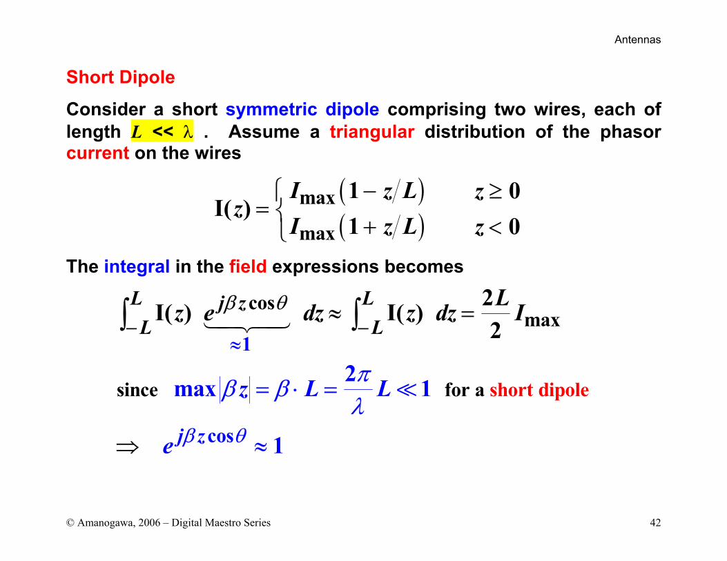
Short Dipole
Consider a short symmetric dipole comprising two wires, each of length L << λ . Assume a triangular distribution of the phasor current on the wires
The integral in the field expressions becomes
( )( )
max
max
1 0I( )
1 0I z L z
zI z L z
− ≥= + <
cosmax
since short
1
dipolefor a
cos
2max 1
1
2I( ) I( )2
z
L LjL L
j
z Lz e dz z dz
z L L
I
e β
β θ
θ
πβ βλ
−≈
−
= ⋅ =
≈
≈ =
⇒
∫ ∫
Antennas
© Amanogawa, 2006 – Digital Maestro Series 43
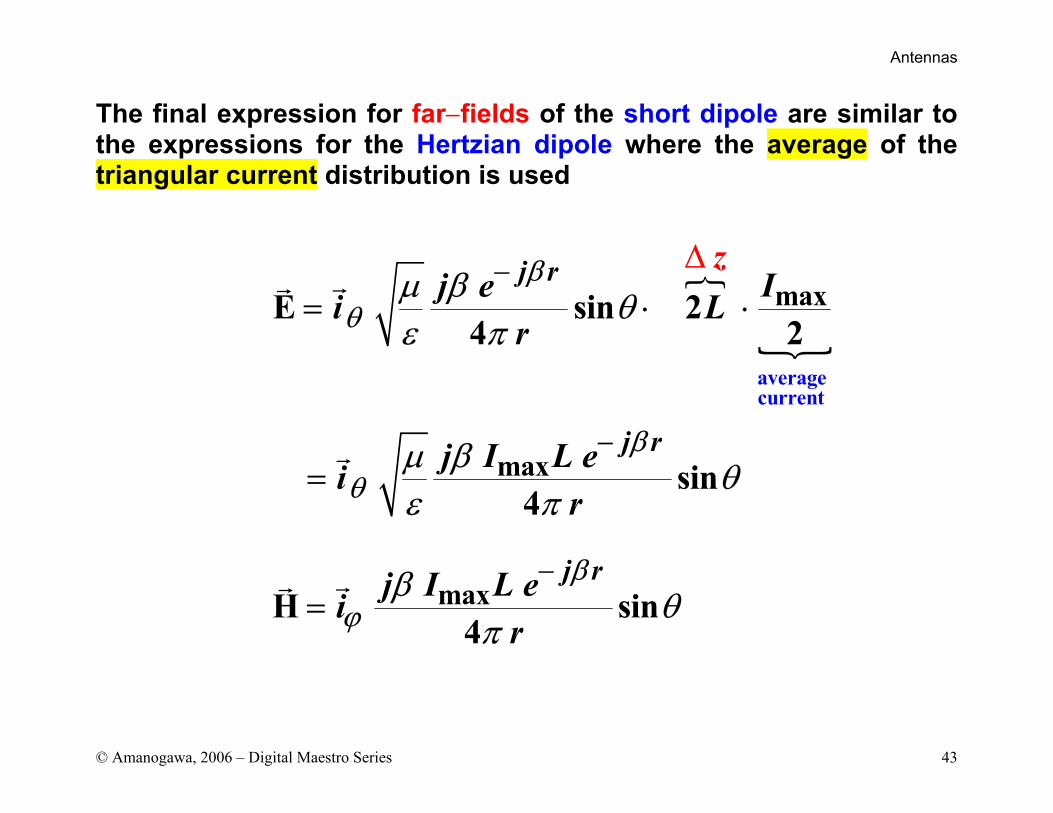
The final expression for far−fields of the short dipole are similar to the expressions for the Hertzian dipole where the average of the triangular current distribution is used
average current
max
max
max
E sin 24 2
sin4
H sin4
j r
j r
j r
j e Ii Lr
j I L eir
j I L eir
zβθ
βθ
βϕ
µ β θε π
µ β θε π
β θπ
−
−
−
= ⋅ ⋅
=
∆
=
Antennas
© Amanogawa, 2006 – Digital Maestro Series 44
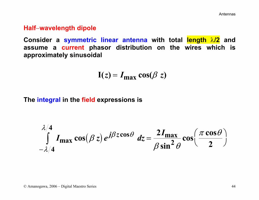
Half−wavelength dipole
Consider a symmetric linear antenna with total length λ/2 and assume a current phasor distribution on the wires which is approximately sinusoidal
The integral in the field expressions is
maxI( ) cos( )z I zβ=
( )4
cos maxmax 2
4
2 coscos cos2sin
j z II z e dzλ
β θ
λ
π θββ θ−
= ∫
Antennas
© Amanogawa, 2006 – Digital Maestro Series 45
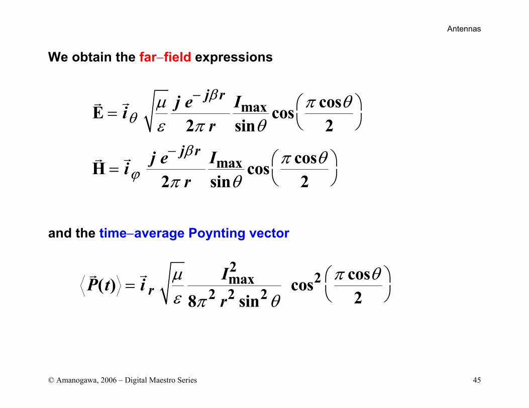
We obtain the far−field expressions
and the time−average Poynting vector
max
max
cosE cos2 sin 2
cosH cos2 sin 2
j r
j r
j e Iir
j e Iir
βθ
βϕ
µ π θε π θ
π θπ θ
−
−
=
=
22max
2 2 2cos( ) cos28 sin
rIP t ir
µ π θε π θ
=
Antennas
© Amanogawa, 2006 – Digital Maestro Series 46
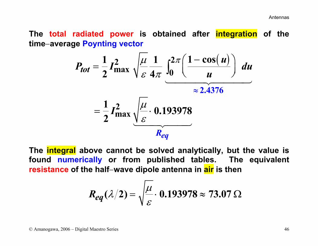
The total radiated power is obtained after integration of the time−average Poynting vector
The integral above cannot be solved analytically, but the value is found numerically or from published tables. The equivalent resistance of the half−wave dipole antenna in air is then
( )
2.4376
22max 0
2max
1 cos1 12 4
1 0.1939782
eq
tot
R
uP I duu
I
πµε π
µε
≈
− =
= ⋅
∫
( 2) 0.193978 73.07eqR µλε
= ⋅ ≈ Ω
Antennas
© Amanogawa, 2006 – Digital Maestro Series 47
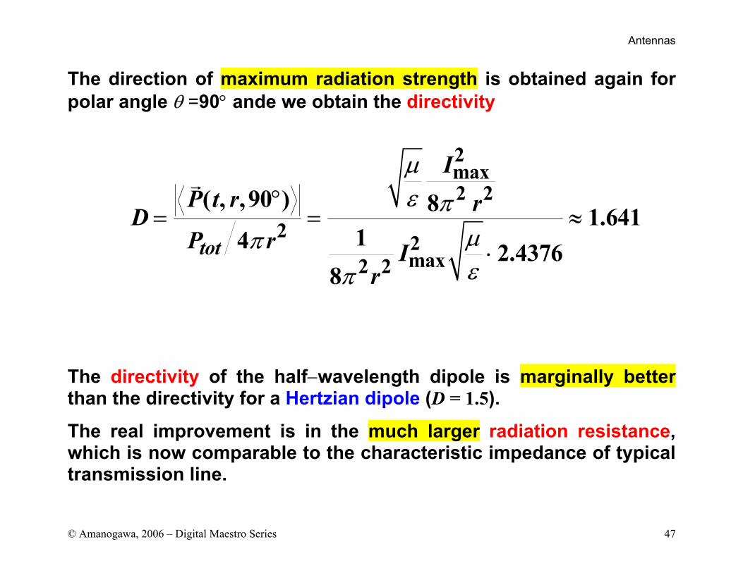
The direction of maximum radiation strength is obtained again for polar angle θ =90° ande we obtain the directivity
The directivity of the half−wavelength dipole is marginally better than the directivity for a Hertzian dipole (D = 1.5).
The real improvement is in the much larger radiation resistance, which is now comparable to the characteristic impedance of typical transmission line.
2max2 2
2 2max2 2
( , ,90 ) 8 1.64114 2.4376
8tot
IP t r rDP r I
r
µε π
µπεπ
°= = ≈
⋅
Antennas
© Amanogawa, 2006 – Digital Maestro Series 48
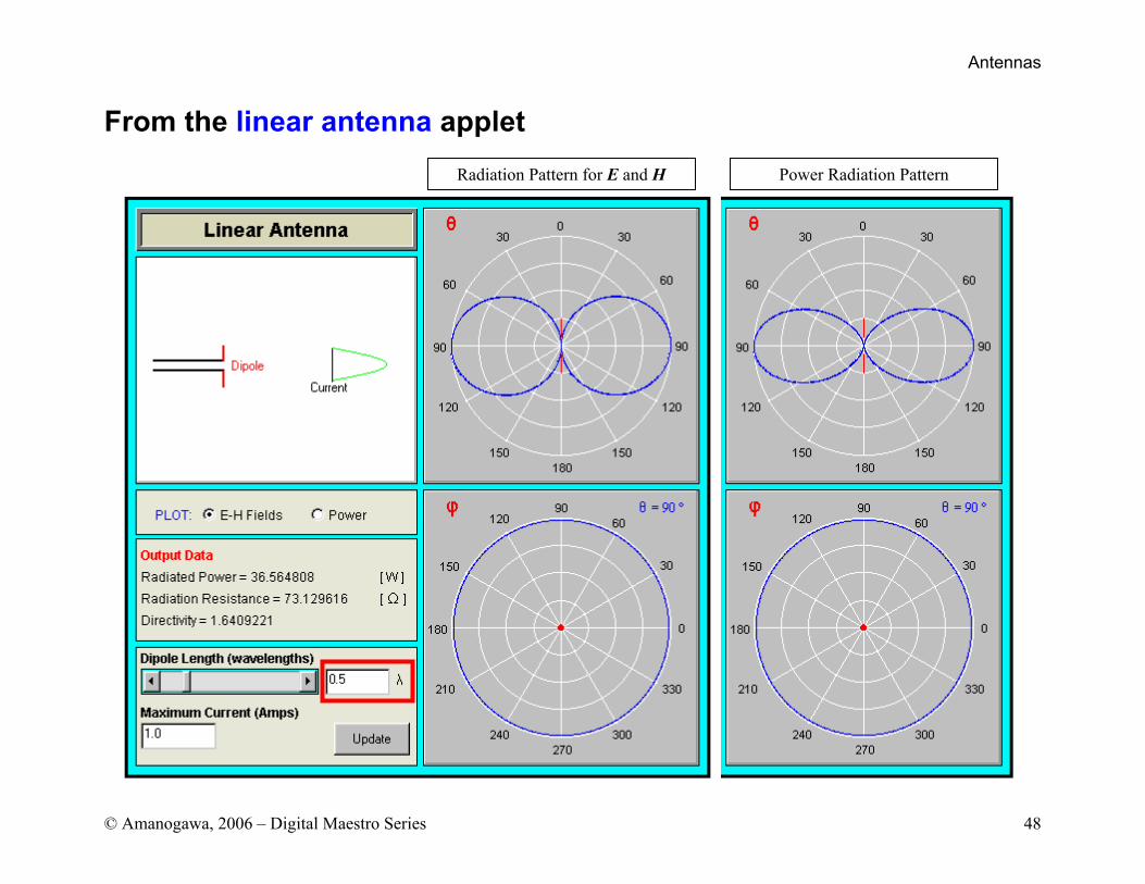
From the linear antenna applet
Radiation Pattern for E and H Power Radiation Pattern
Antennas
© Amanogawa, 2006 – Digital Maestro Series 49
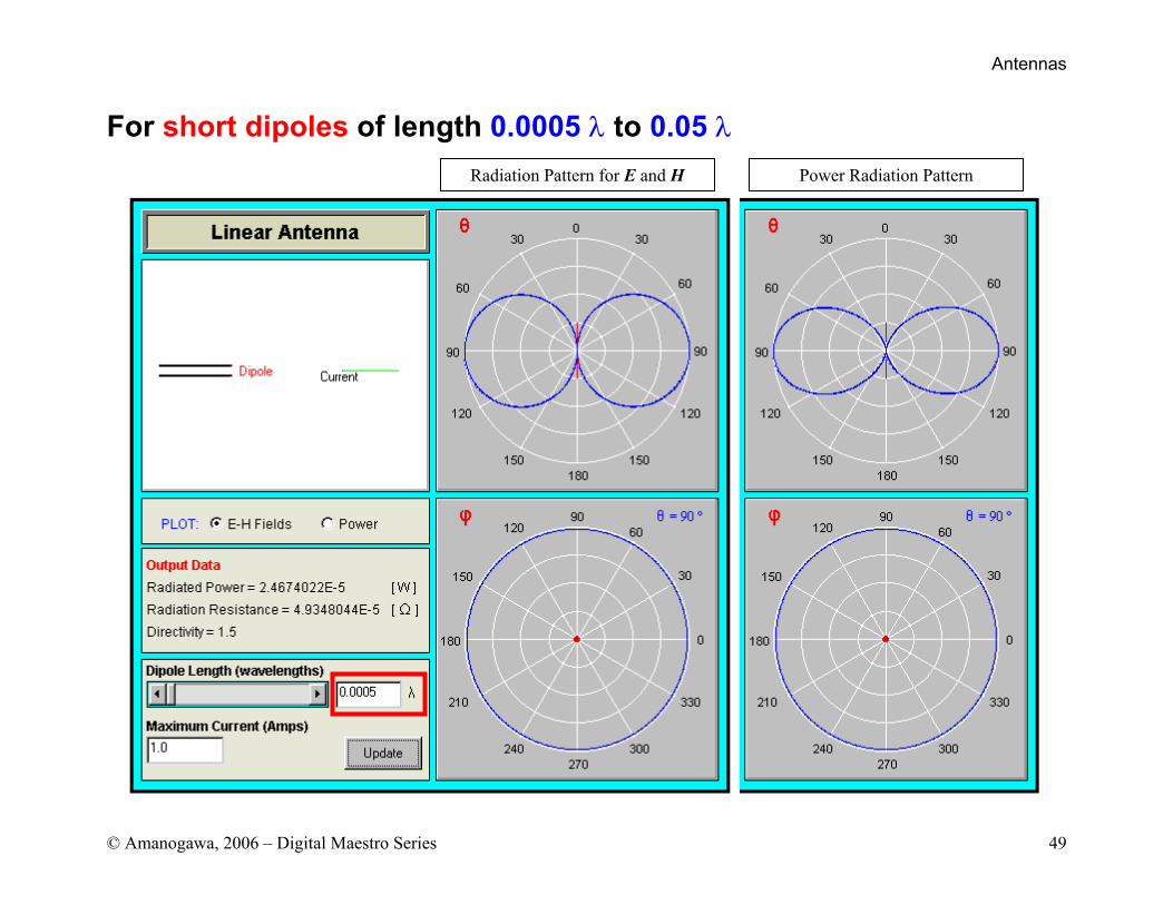
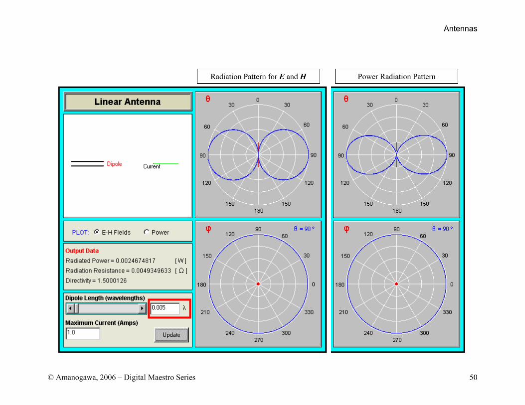
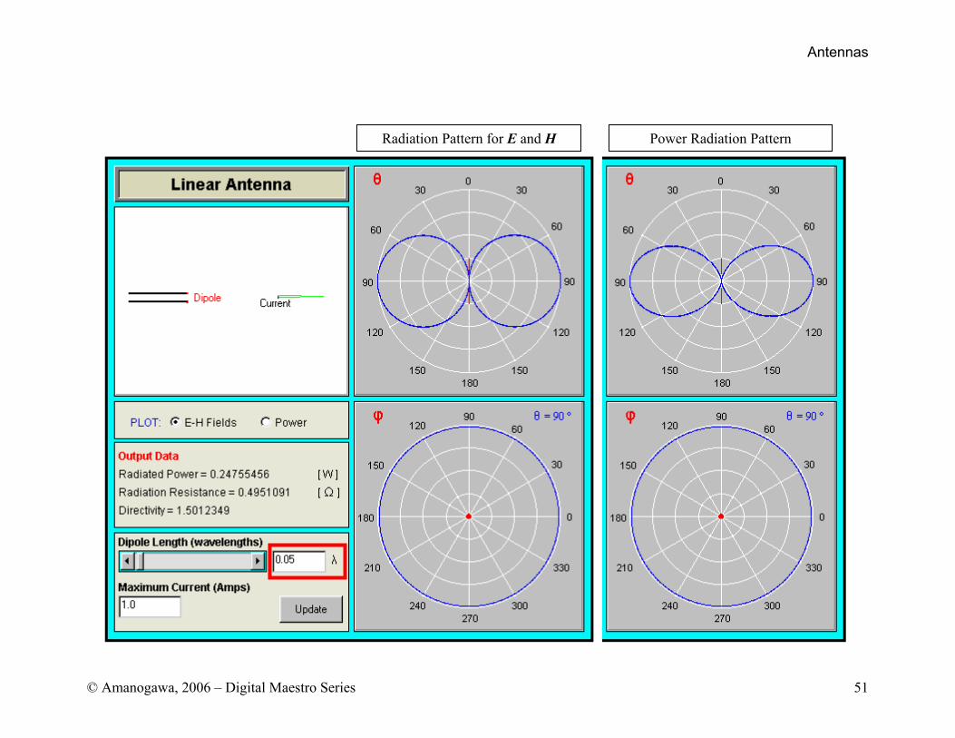
For short dipoles of length 0.0005 λ to 0.05 λ
Radiation Pattern for E and H Power Radiation Pattern
Antennas
© Amanogawa, 2006 – Digital Maestro Series 50
Radiation Pattern for E and H Power Radiation Pattern
Antennas
© Amanogawa, 2006 – Digital Maestro Series 51
Radiation Pattern for E and H Power Radiation Pattern
Antennas
© Amanogawa, 2006 – Digital Maestro Series 52
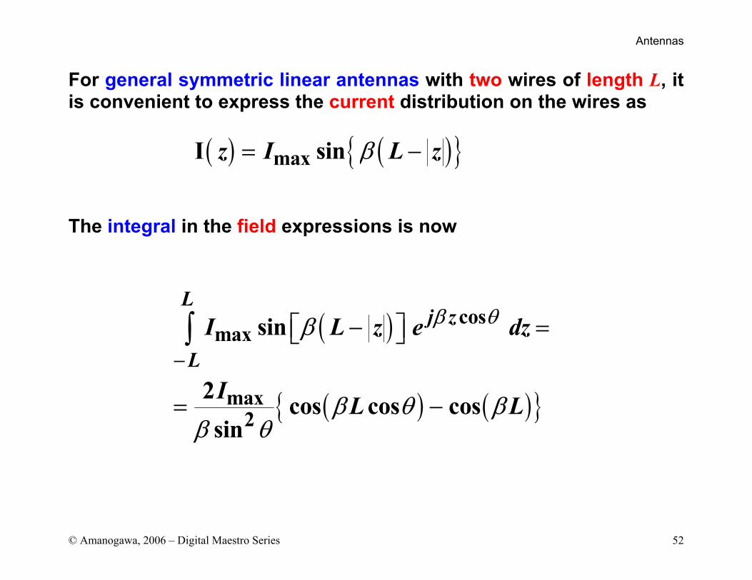
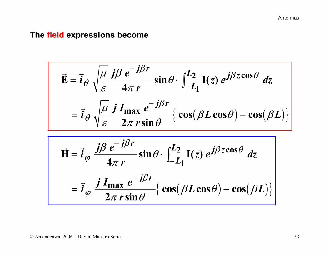
For general symmetric linear antennas with two wires of length L, it is convenient to express the current distribution on the wires as
The integral in the field expressions is now
( ) ( ) maxI sinz I L zβ= −
( )
( ) ( )
cosmax
max2
sin
2 cos cos cossin
Lj z
LI L z e dz
I L L
β θβ
β θ ββ θ
−− =
= −
∫
Antennas
© Amanogawa, 2006 – Digital Maestro Series 53
The field expressions become
( ) ( )
( ) ( )
21
21
cos
max
cos
max
E sin I( )4
cos cos cos2 sin
H sin I( )4
cos cos cos2 sin
j r L j zL
j r
j r L j zL
j r
j ei z e dzr
j I ei L Lr
j ei z e dzr
j I ei L Lr
ββ θ
θ
βθ
ββ θ
ϕ
βϕ
µ β θε π
µ β θ βε π θ
β θπ
β θ βπ θ
−
−
−
−
−
−
= ⋅
= −
= ⋅
= −
∫
∫
Antennas
© Amanogawa, 2006 – Digital Maestro Series 54
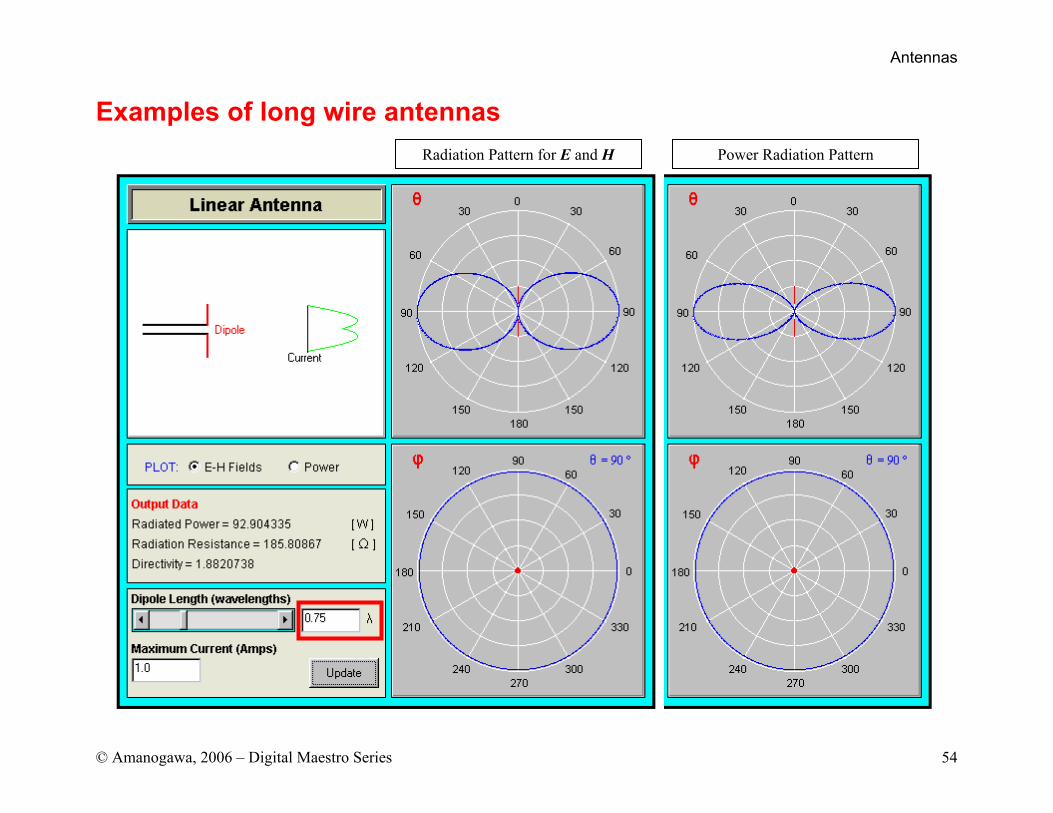
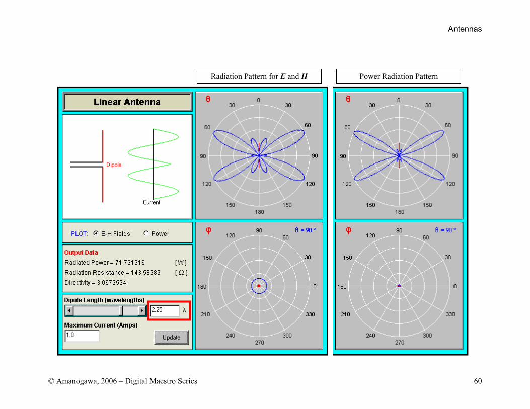
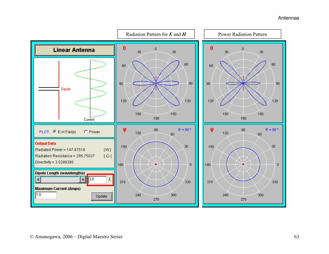
Examples of long wire antennas
Radiation Pattern for E and H Power Radiation Pattern

Antennas
© Amanogawa, 2006 – Digital Maestro Series 55
Radiation Pattern for E and H Power Radiation Pattern
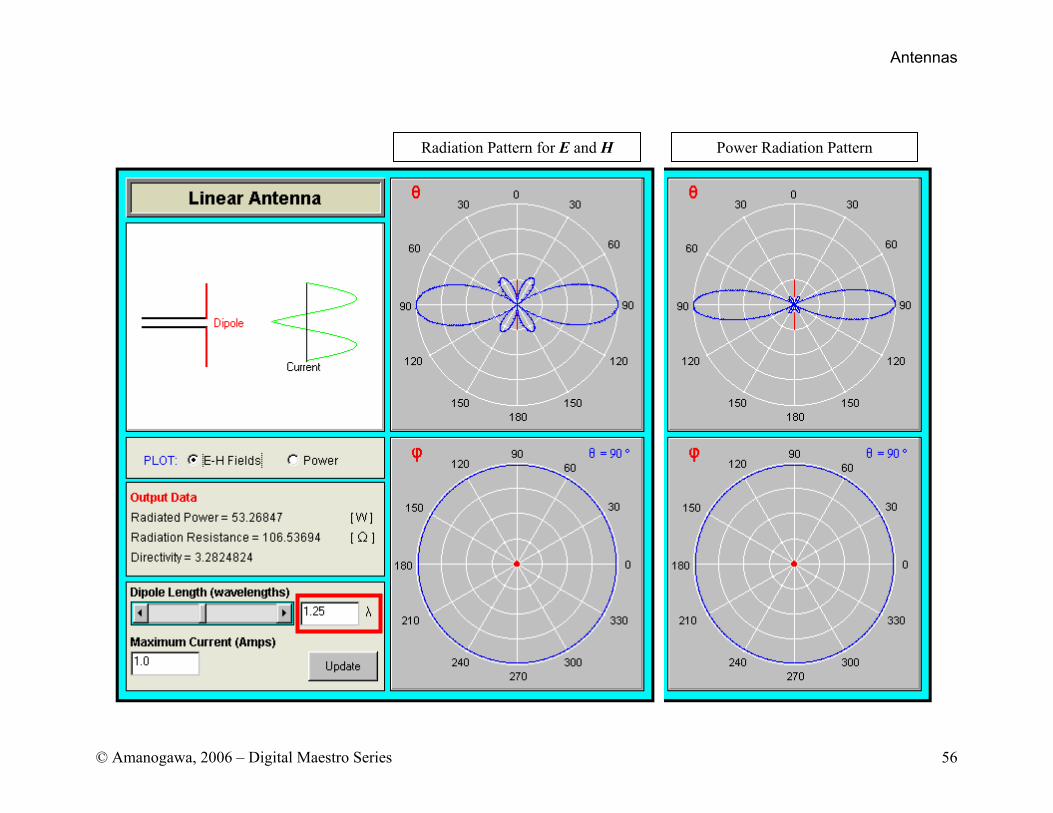
Antennas
© Amanogawa, 2006 – Digital Maestro Series 56
Radiation Pattern for E and H Power Radiation Pattern

Antennas
© Amanogawa, 2006 – Digital Maestro Series 57
Radiation Pattern for E and H Power Radiation Pattern

Antennas
© Amanogawa, 2006 – Digital Maestro Series 58
Radiation Pattern for E and H Power Radiation Pattern
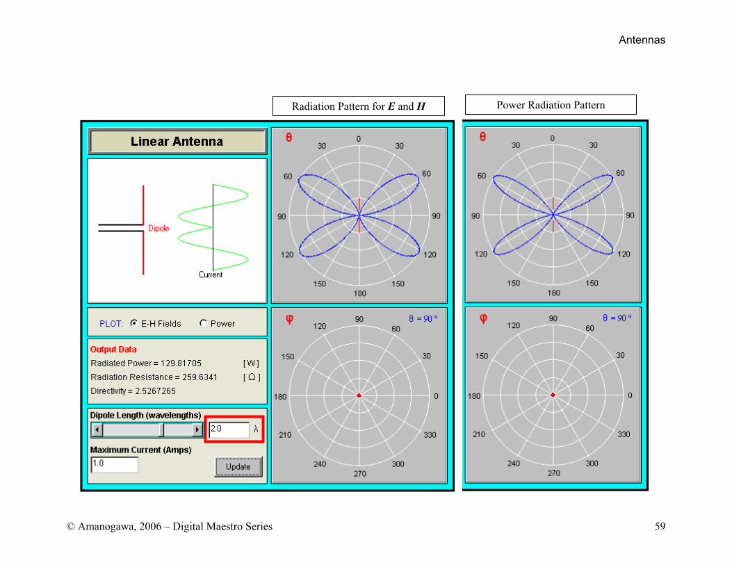
Antennas
© Amanogawa, 2006 – Digital Maestro Series 59
Radiation Pattern for E and H Power Radiation Pattern
Antennas
© Amanogawa, 2006 – Digital Maestro Series 60
Radiation Pattern for E and H Power Radiation Pattern
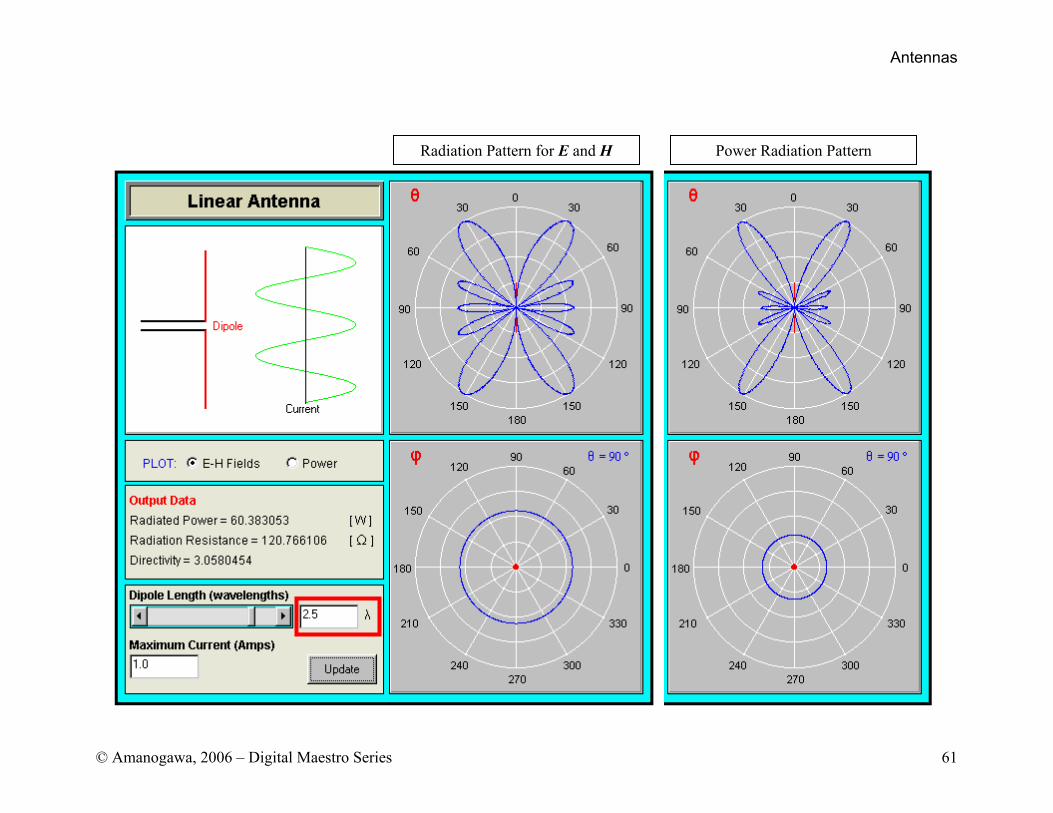
Antennas
© Amanogawa, 2006 – Digital Maestro Series 61
Radiation Pattern for E and H Power Radiation Pattern

Antennas
© Amanogawa, 2006 – Digital Maestro Series 62
Radiation Pattern for E and H Power Radiation Pattern
Antennas
© Amanogawa, 2006 – Digital Maestro Series 63
Radiation Pattern for E and H Power Radiation Pattern