antennas 97 aperture antennas - ntutjuiching/antenna4.pdf · antennas 97 aperture antennas...
TRANSCRIPT

Antennas 97
Aperture Antennas
Reflectors, horns.High GainNearly real input impedance
Huygens’ Principle
Each point of a wave front is a secondary source of spherical waves.
97

Antennas 98
Equivalence Principle
Uniqueness Theorem: a solution satisfying Maxwell’s Equations andthe boundary conditions is unique.
1. Original Problem (a): 2. Equivalent Problem (b): outside , inside ,
on , where
3. Equivalent Problem (c): outside , zero fields inside , on , where
To further simplify,Case 1: PEC. No contribution from .
Case 2: PMC. No contribution from .
Infinite Planar Surface
98

Antennas 99
To calculate the fields, first find the vector potential due to theequivalent electric and magnetic currents.
In the far field, from Eqs. (1-105),
Since in the far field, the fields can be approximate by spherical TEMwaves,
99
Antennas 100
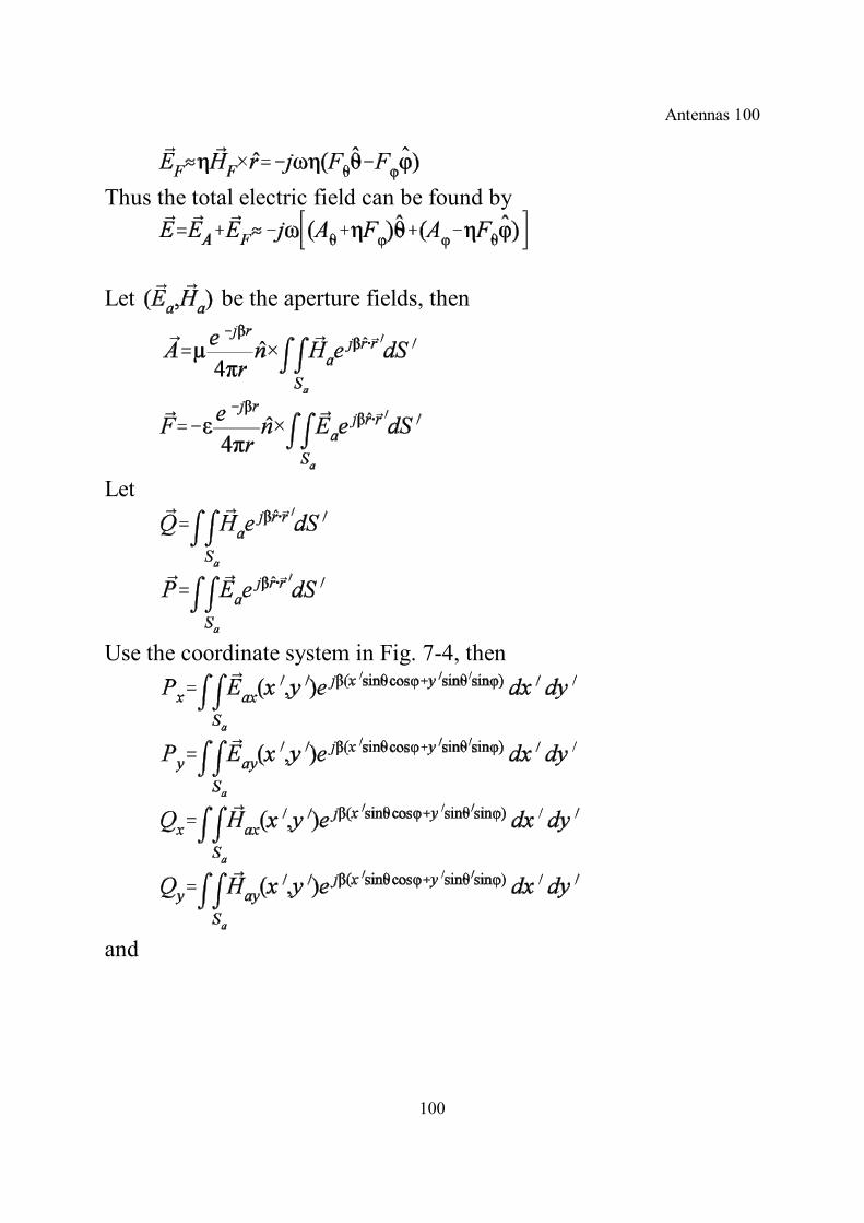
Thus the total electric field can be found by
Let be the aperture fields, then
Let
Use the coordinate system in Fig. 7-4, then
and
100

Antennas 101
or in spherical coordinate system
Using Eq. (7-8), we have
If the aperture fields are TEM waves, then
This implies
Full Vector Form
101
Antennas 102
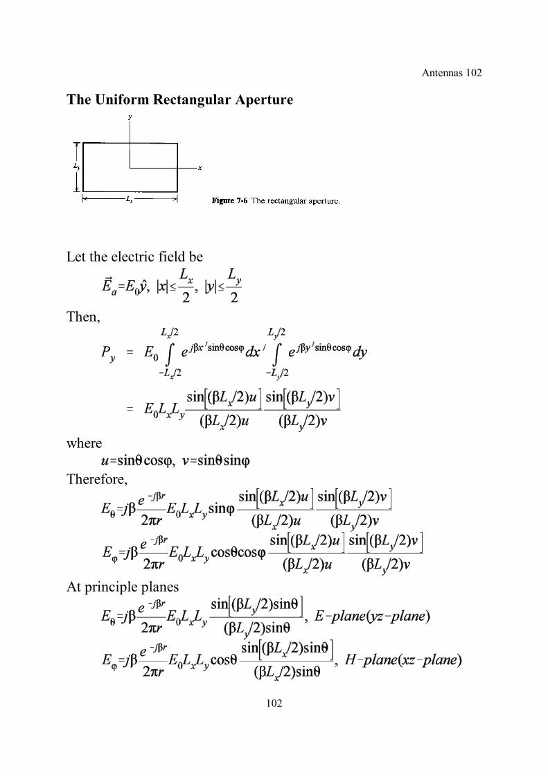
The Uniform Rectangular Aperture
Let the electric field be
Then,
where
Therefore,
At principle planes
102

Antennas 103
For large aperture ( ), the main beam is narrow, the factor is negligible. The half-power beam width
.
Also,
Example: a Uniform Rectangular Aperture
103

Antennas 104
104

Antennas 105
105

Antennas 106
Techniques for Evaluating Gain
Directivity
From (7-27), (7-24), (7-61)
Thus, for broadside case,
Total power
Then,
In general, for uniform distribution
If
then
where are the directivity of a line source due to respectively. the main beam direction relative to broadside.
106
Antennas 107
Directivity of an Open-Ended Rectangular Waveguide:
Gain and Efficiencies
where : aperture efficiency
: radiation efficiency. (~1 for aperture antennas)
: taper efficiency or utilization factor.
: spillover efficiency. is called : illumination efficiency.: achievement efficiency. : cross-polarization
efficiency. phase-error efficiency.
Beam efficiency
Simple Directivity Formulas in Terms of HP beam width
1. Low directivity, no sidelobe
2. Large electrical size
107

Antennas 108
3. High gain
Example 7-5: Pyramidal Horn Antenna (aperture efficiency=0.51)Measured gained at 40 GHz: 24.7 dB.A=5.54 cm, B=4.55 cm.
Example 7-6: Circular Parabolic Reflector AntennaTypical aperture efficiency: 55%.Diameter: 3.66 mFrequency: 11.7 GHzMeasured Gain: 50.4 dB.Measured .
1. Computed by aperture efficiency
2. Computed by half power beam width
108
Antennas 109
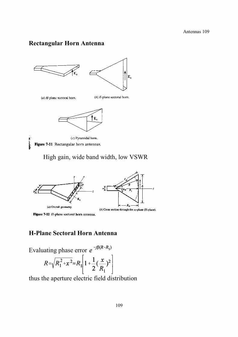
Rectangular Horn Antenna
High gain, wide band width, low VSWR
H-Plane Sectoral Horn Antenna
Evaluating phase error
thus the aperture electric field distribution
109

Antennas 110
where is defined in (7-108), (7-109)
Directivity
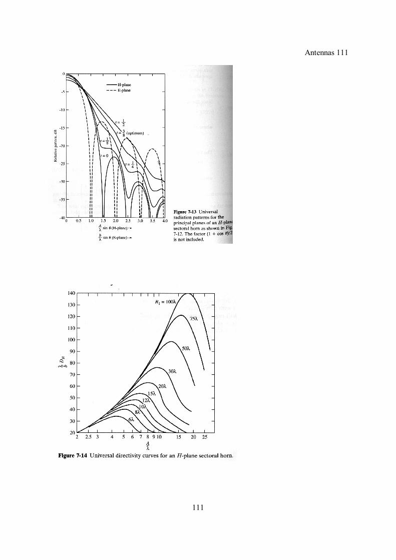
Figure 7-13: universal E-plane and H-plane pattern with
factor omitted, and (a measure of the maximum phase
error at the edge)
Figure 7-14: Universal directivity curves.
Optimum directivity occurs at and
From figure 7.13 for optimum case,
110
Antennas 111
111
Antennas 112
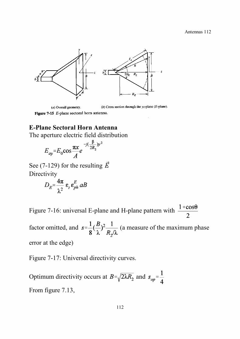
E-Plane Sectoral Horn AntennaThe aperture electric field distribution
See (7-129) for the resulting Directivity
Figure 7-16: universal E-plane and H-plane pattern with
factor omitted, and (a measure of the maximum phase
error at the edge)
Figure 7-17: Universal directivity curves.
Optimum directivity occurs at and
From figure 7.13,
112

Antennas 113
113

Antennas 114
Pyramidal Horn Antenna
The aperture electric field distribution
At optimum condition:
Optimum gain
For non optimum case,
Design procedure:1. Specify gain , wavelength , waveguide dimension , .
114
Antennas 115
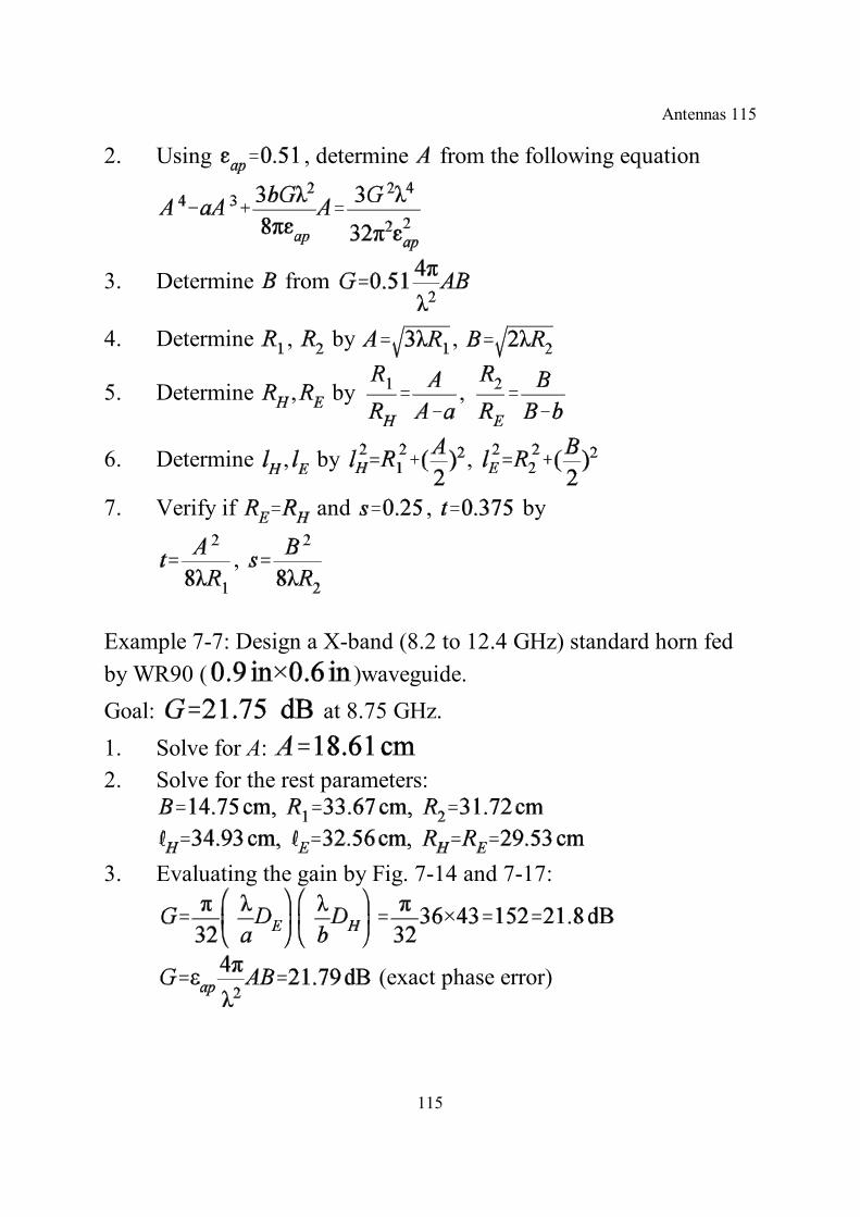
2. Using , determine from the following equation
3. Determine from
4. Determine , by ,
5. Determine , by ,
6. Determine , by ,
7. Verify if and , by
,
Example 7-7: Design a X-band (8.2 to 12.4 GHz) standard horn fedby WR90 ( )waveguide.Goal: at 8.75 GHz.1. Solve for A: 2. Solve for the rest parameters:
3. Evaluating the gain by Fig. 7-14 and 7-17:
(exact phase error)
115
Antennas 116
116

Antennas 117
117

Antennas 118
118

Antennas 119
Reflector AntennasParabolic Reflector
Parabolic equation:
or
Properties1. Focal point at . All rays leaving , will be parallel after
reflection from the parabolic surface.2. All path lengths from the focal point to any aperture plane are
equal.3. To determine the radiation pattern, find the field distribution at
the aperture plane using GO.Geometrical Optics (GO)
119
Antennas 120
Requirements1. The radius curvature of the reflector is large compared to a
wavelength, allowing planar approximation.2. The radius curvature of the incoming wave from the feed is
large, allowing planar approximation.3. The reflector is a perfect conductor, thus the reflect coefficient
.
Parabolic reflector:Wideband.Lower limit determine by the size of the reflector. Should be
several wavelengths for GO to hold.Higher limit determine by the surface roughness of the reflector.
Should much smaller than a wavelength.Also limited by the bandwidth of the feed.
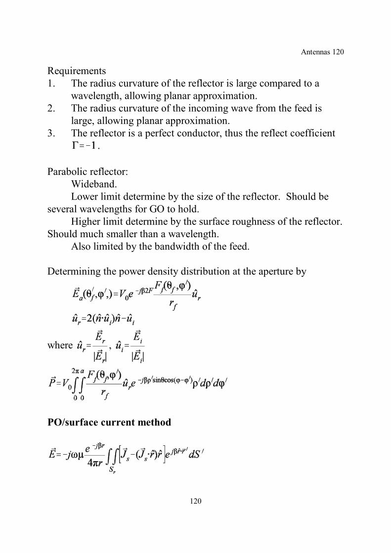
Determining the power density distribution at the aperture by
where ,
PO/surface current method
120

Antennas 121
PO and GO both yield good patterns in main beam and first fewsidelobes. Deteriorate due to diffraction by the edge of the reflector.PO is better than GO for offset reflectors.
Axis-symmetric Parabolic Reflector Antenna
For a linear polarized feed along x-axis, the pattern can beapproximate by the two principle plan patterns as below.
where , are E-plane and H-plane patterns.
If the pattern is rotationally symmetric, then . We have
Also, the cross-polarization of the aperture field is maximum in the. Leads to cross-polarization.
For a short dipole, , ,
At , only x component exists.
121
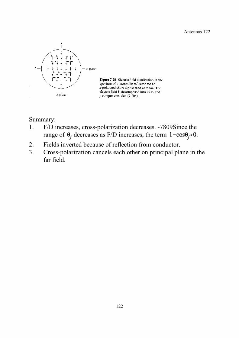
Antennas 122
Summary:1. F/D increases, cross-polarization decreases. -7809Since the
range of decreases as F/D increases, the term . 2. Fields inverted because of reflection from conductor.3. Cross-polarization cancels each other on principal plane in the
far field.
122

Antennas 123
123
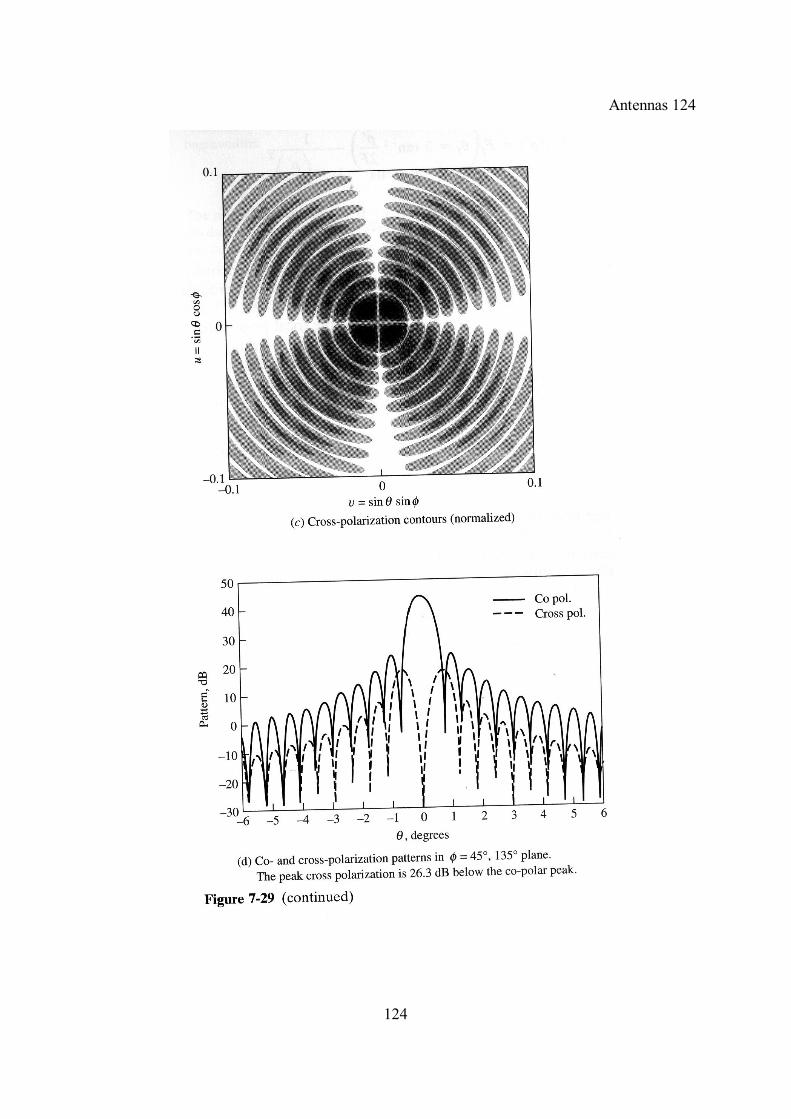
Antennas 124
124

Antennas 125
Approximation formula
Normalized aperture field
Thus, (7-208)
whereEI=edge illumination (dB) =20 log CET=edge taper (dB)=-EIFT=feed taper (at aperture edge) (dB)=Spherical spreading loss at the aperture edge
Design procedure of axial symmetrical aperture field:1. Estimate EI by the radiation pattern of the feed at the edge angle
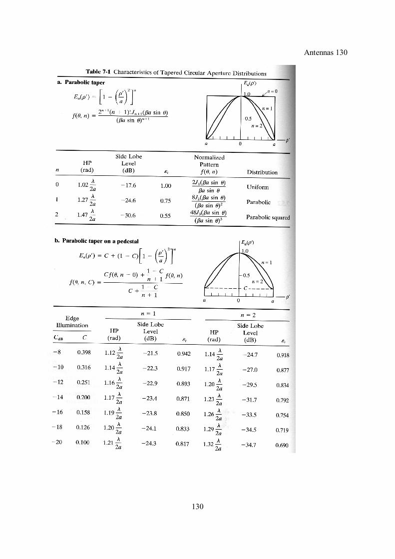
of the reflector.2. Calculate due to the distance from the feed to the edge.3. Estimate ET at the aperture by adding the EI and . 4. Look up Table 7-1 for a suitable n.
Example 7-8: A 28-GHz Parabolic Reflector Antenna fed by circularcorrugated horn.
125

Antennas 126
Assume , then
Use Table 7.1b for n=2 and interpolate, we have
( measured)
( measured)
126
Antennas 127
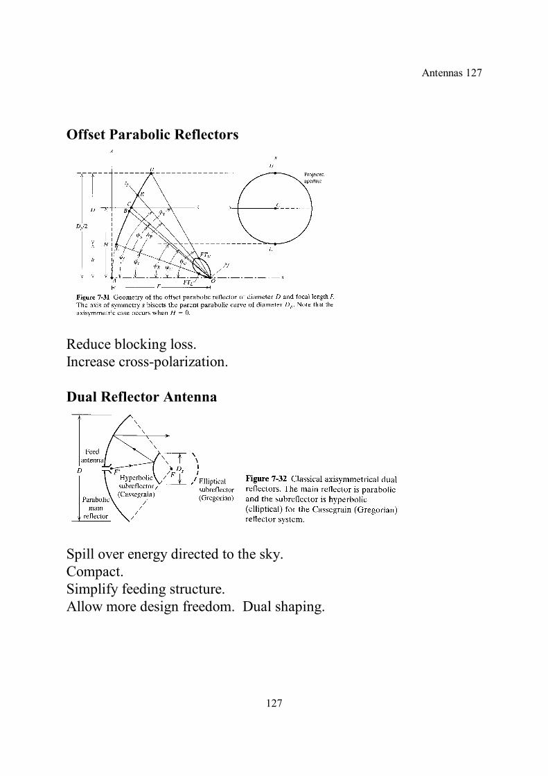
Offset Parabolic Reflectors
Reduce blocking loss.Increase cross-polarization.
Dual Reflector Antenna
Spill over energy directed to the sky.Compact.Simplify feeding structure.Allow more design freedom. Dual shaping.
127

Antennas 128
Other types
Design example1. Determine the reflector diameter by half-power beam width.
For the optimum -11 dB edge illumination,
(7-248)
2. Choose F/D. Usually between 0.3 to 1.0.3. Determine the required feed pattern using model.
(7-249)
Example 7-9: From 7-248
128
Antennas 129
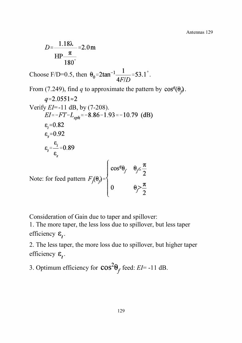
Choose F/D=0.5, then .
From (7.249), find q to approximate the pattern by .
Verify EI=-11 dB, by (7-208).
Note: for feed pattern
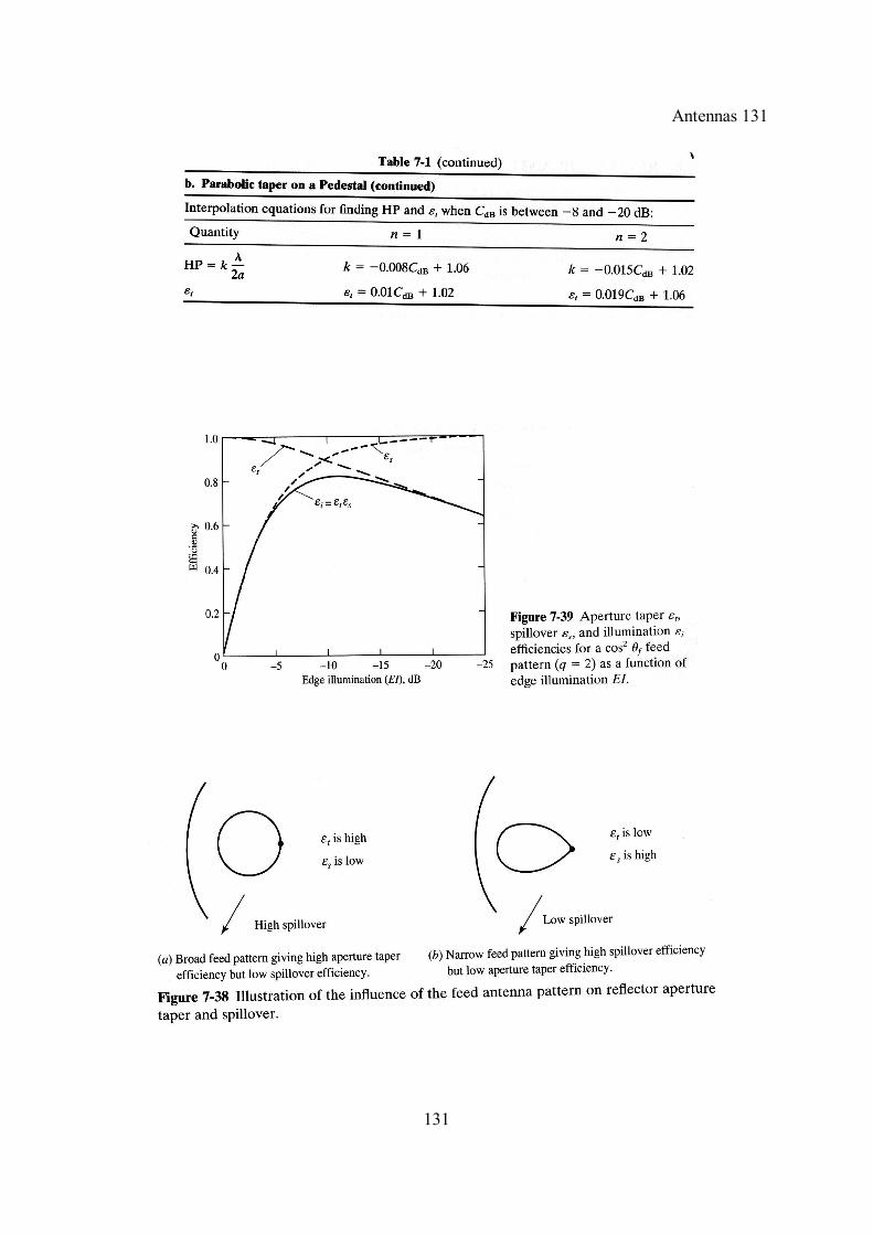
Consideration of Gain due to taper and spillover:1. The more taper, the less loss due to spillover, but less taperefficiency .
2. The less taper, the more loss due to spillover, but higher taperefficiency .
3. Optimum efficiency for feed: EI= -11 dB.
129
Antennas 130
130
Antennas 131
131

Antennas 132
132
Antennas 133
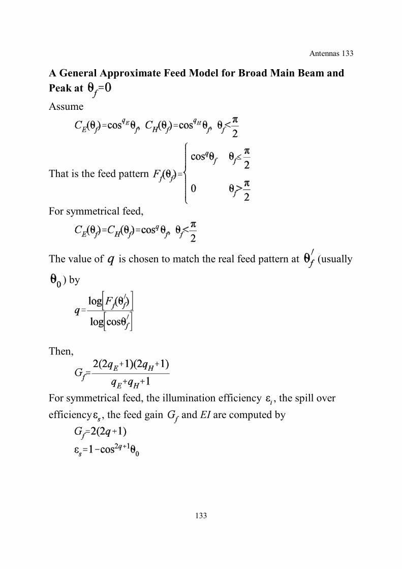
A General Approximate Feed Model for Broad Main Beam andPeak at
Assume
That is the feed pattern
For symmetrical feed,
The value of is chosen to match the real feed pattern at (usually
) by
Then,
For symmetrical feed, the illumination efficiency , the spill overefficiency , the feed gain and EI are computed by
133

Antennas 134
134

Antennas 135
135