answers to exercises - home - springer978-1-84628-603...answers to exercises a bird does not sing...
TRANSCRIPT

Answers to Exercises
A bird does not sing because he has an answer, he sings because he has a song.—Chinese Proverb
Intro.1: abstemious, abstentious, adventitious, annelidous, arsenious, arterious, face-tious, sacrilegious.
Intro.2: When a software house has a popular product they tend to come up withnew versions. A user can update an old version to a new one, and the update usuallycomes as a compressed file on a floppy disk. Over time the updates get bigger and, at acertain point, an update may not fit on a single floppy. This is why good compression isimportant in the case of software updates. The time it takes to compress and decompressthe update is unimportant since these operations are typically done just once. Recently,software makers have taken to providing updates over the Internet, but even in suchcases it is important to have small files because of the download times involved.
1.1: (1) ask a question, (2) absolutely necessary, (3) advance warning, (4) boilinghot, (5) climb up, (6) close scrutiny, (7) exactly the same, (8) free gift, (9) hot waterheater, (10) my personal opinion, (11) newborn baby, (12) postponed until later, (13)unexpected surprise, (14) unsolved mysteries.
1.2: A reasonable way to use them is to code the five most-common strings in thetext. Because irreversible text compression is a special-purpose method, the user mayknow what strings are common in any particular text to be compressed. The user mayspecify five such strings to the encoder, and they should also be written at the start ofthe output stream, for the decoder’s use.
1.3: 6,8,0,1,3,1,4,1,3,1,4,1,3,1,4,1,3,1,2,2,2,2,6,1,1. The first two are the bitmap reso-lution (6×8). If each number occupies a byte on the output stream, then its size is 25bytes, compared to a bitmap size of only 6 × 8 bits = 6 bytes. The method does notwork for small images.

954 Answers to Exercises
1.4: RLE of images is based on the idea that adjacent pixels tend to be identical. Thelast pixel of a row, however, has no reason to be identical to the first pixel of the nextrow.
1.5: Each of the first four rows yields the eight runs 1,1,1,2,1,1,1,eol. Rows 6 and 8yield the four runs 0,7,1,eol each. Rows 5 and 7 yield the two runs 8,eol each. The totalnumber of runs (including the eol’s) is thus 44.
When compressing by columns, columns 1, 3, and 6 yield the five runs 5,1,1,1,eoleach. Columns 2, 4, 5, and 7 yield the six runs 0,5,1,1,1,eol each. Column 8 gives 4,4,eol,so the total number of runs is 42. This image is thus “balanced” with respect to rowsand columns.
1.6: The result is five groups as follows:
W1 to W2 :00000, 11111,
W3 to W10 :00001, 00011, 00111, 01111, 11110, 11100, 11000, 10000,
W11 to W22 :00010, 00100, 01000, 00110, 01100, 01110,
11101, 11011, 10111, 11001, 10011, 10001,
W23 to W30 :01011, 10110, 01101, 11010, 10100, 01001, 10010, 00101,
W31 to W32 :01010, 10101.
1.7: The seven codes are
0000, 1111, 0001, 1110, 0000, 0011, 1111,
forming a string with six runs. Applying the rule of complementing yields the sequence
0000, 1111, 1110, 1110, 0000, 0011, 0000,
with seven runs. The rule of complementing does not always reduce the number of runs.
1.8: As “11 22 90 00 00 33 44”. The 00 following the 90 indicates no run, and thefollowing 00 is interpreted as a regular character.
1.9: The six characters “123ABC” have ASCII codes 31, 32, 33, 41, 42, and 43. Trans-lating these hexadecimal numbers to binary produces “00110001 00110010 0011001101000001 01000010 01000011”.The next step is to divide this string of 48 bits into 6-bit blocks. They are 001100=12,010011=19, 001000=8, 110011=51, 010000=16, 010100=20, 001001=9, and 000011=3.The character at position 12 in the BinHex table is “-” (position numbering starts atzero). The one at position 19 is “6”. The final result is the string “-6)c38*$”.
1.10: Exercise 2.1 shows that the binary code of the integer i is 1 + �log2 i� bits long.We add �log2 i� zeros, bringing the total size to 1 + 2�log2 i� bits.

Answers to Exercises 955
1.11: Table Ans.1 summarizes the results. In (a), the first string is encoded with k = 1.In (b) it is encoded with k = 2. Columns (c) and (d) are the encodings of the secondstring with k = 1 and k = 2, respectively. The averages of the four columns are 3.4375,3.25, 3.56, and 3.6875; very similar! The move-ahead-k method used with small valuesof k does not favor strings satisfying the concentration property.
a abcdmnop 0b abcdmnop 1c bacdmnop 2d bcadmnop 3d bcdamnop 2c bdcamnop 2b bcdamnop 0a bcdamnop 3m bcadmnop 4n bcamdnop 5o bcamndop 6p bcamnodp 7p bcamnopd 6o bcamnpod 6n bcamnopd 4m bcanmopd 4
bcamnopd
(a)
a abcdmnop 0b abcdmnop 1c bacdmnop 2d cbadmnop 3d cdbamnop 1c dcbamnop 1b cdbamnop 2a bcdamnop 3m bacdmnop 4n bamcdnop 5o bamncdop 6p bamnocdp 7p bamnopcd 5o bampnocd 5n bamopncd 5m bamnopcd 2
mbanopcd
(b)
a abcdmnop 0b abcdmnop 1c bacdmnop 2d bcadmnop 3m bcdamnop 4n bcdmanop 5o bcdmnaop 6p bcdmnoap 7a bcdmnopa 7b bcdmnoap 0c bcdmnoap 1d cbdmnoap 2m cdbmnoap 3n cdmbnoap 4o cdmnboap 5p cdmnobap 7
cdmnobpa
(c)
a abcdmnop 0b abcdmnop 1c bacdmnop 2d cbadmnop 3m cdbamnop 4n cdmbanop 5o cdmnbaop 6p cdmnobap 7a cdmnopba 7b cdmnoapb 7c cdmnobap 0d cdmnobap 1m dcmnobap 2n mdcnobap 3o mndcobap 4p mnodcbap 7
mnodcpba
(d)
Table Ans.1: Encoding With Move-Ahead-k.
1.12: Table Ans.2 summarizes the decoding steps. Notice how similar it is to Ta-ble 1.16, indicating that move-to-front is a symmetric data compression method.
Code input A (before adding) A (after adding) Word
0the () (the) the1boy (the) (the, boy) boy2on (boy, the) (boy, the, on) on3my (on, boy, the) (on, boy, the, my) my4right (my, on, boy, the) (my, on, boy, the, right) right5is (right, my, on, boy, the) (right, my, on, boy, the, is) is5 (is, right, my, on, boy, the) (is, right, my, on, boy, the) the2 (the, is, right, my, on, boy) (the, is, right, my, on, boy) right5 (right, the, is, my, on, boy) (right, the, is, my, on, boy) boy
(boy, right, the, is, my, on)
Table Ans.2: Decoding Multiple-Letter Words.

956 Answers to Exercises
2.1: It is 1 + �log2 i� as can be seen by simple experimenting.
2.2: The integer 2 is the smallest integer that can serve as the basis for a numbersystem.
2.3: Replacing 10 by 3 we get x = k log2 3 ≈ 1.58k. A trit is therefore worth about1.58 bits.
2.4: We assume an alphabet with two symbols a1 and a2, with probabilities P1 andP2, respectively. Since P1 + P2 = 1, the entropy of the alphabet is −P1 log2 P1 − (1 −P1) log2(1−P1). Table Ans.3 shows the entropies for certain values of the probabilities.When P1 = P2, at least 1 bit is required to encode each symbol, reflecting the factthat the entropy is at its maximum, the redundancy is zero, and the data cannot becompressed. However, when the probabilities are very different, the minimum numberof bits required per symbol drops significantly. We may not be able to develop a com-pression method using 0.08 bits per symbol but we know that when P1 = 99%, this isthe theoretical minimum.
P1 P2 Entropy99 1 0.0890 10 0.4780 20 0.7270 30 0.8860 40 0.9750 50 1.00
Table Ans.3: Probabilities and Entropies of Two Symbols.
An essential tool of this theory [information] is a quantity for measuring theamount of information conveyed by a message. Suppose a message is encoded intosome long number. To quantify the information content of this message, Shannonproposed to count the number of its digits. According to this criterion, 3.14159, forexample, conveys twice as much information as 3.14, and six times as much as 3.Struck by the similarity between this recipe and the famous equation on Boltzman’stomb (entropy is the number of digits of probability), Shannon called his formula the“information entropy.”
Hans Christian von Baeyer, Maxwell’s Demon (1998)
2.5: It is easy to see that the unary code satisfies the prefix property, so it definitely canbe used as a variable-size code. Since its length L satisfies L = n we get 2−L = 2−n, so itmakes sense to use it in cases were the input data consists of integers n with probabilitiesP (n) ≈ 2−n. If the data lends itself to the use of the unary code, the entire Huffmanalgorithm can be skipped, and the codes of all the symbols can easily and quickly beconstructed before compression or decompression starts.

Answers to Exercises 957
2.6: The triplet (n, 1, n) defines the standard n-bit binary codes, as can be verified bydirect construction. The number of such codes is easily seen to be
2n+1 − 2n
21 − 1= 2n.
The triplet (0, 0,∞) defines the codes 0, 10, 110, 1110,. . .which are the unary codesbut assigned to the integers 0, 1, 2,. . . instead of 1, 2, 3,. . . .
2.7: The triplet (1, 1, 30) produces (230 − 21)/(21 − 1) ≈ A billion codes.
2.8: This is straightforward. Table Ans.4 shows the code. There are only three differentcodewords since “start” and “stop” are so close, but there are many codes since “start”is large.
a = nth Number of Range ofn 10 + n · 2 codeword codewords integers
0 10 0 x...x︸︷︷︸10
210 = 1K 0–1023
1 12 10 xx...x︸ ︷︷ ︸12
212 = 4K 1024–5119
2 14 11 xx...xx︸ ︷︷ ︸14
214 = 16K 5120–21503
Total 21504
Table Ans.4: The General Unary Code (10,2,14).
2.9: Each part of C4 is the standard binary code of some integer, so it starts with a1. A part that starts with a 0 therefore signals to the decoder that this is the last bit ofthe code.
2.10: We use the property that the Fibonacci representation of an integer does nothave any adjacent 1’s. If R is a positive integer, we construct its Fibonacci representationand append a 1-bit to the result. The Fibonacci representation of the integer 5 is 001,so the Fibonacci-prefix code of 5 is 0011. Similarly, the Fibonacci representation of 33 is1010101, so its Fibonacci-prefix code is 10101011. It is obvious that each of these codesends with two adjacent 1’s, so they can be decoded uniquely. However, the property ofnot having adjacent 1’s restricts the number of binary patterns available for such codes,so they are longer than the other codes shown here.
2.11: Subsequent splits can be done in different ways, but Table Ans.5 shows one wayof assigning Shannon-Fano codes to the 7 symbols.The average size in this case is 0.25 × 2 + 0.20 × 3 + 0.15 × 3 + 0.15 × 2 + 0.10 × 3 +0.10× 4 + 0.05× 4 = 2.75 bits/symbols.
2.12: The entropy is −2(0.25×log2 0.25)− 4(0.125× log2 0.125) = 2.5.

958 Answers to Exercises
Prob. Steps Final
1. 0.25 1 1 :112. 0.20 1 0 :1013. 0.15 1 0 :1004. 0.15 0 1 :015. 0.10 0 0 1 :0016. 0.10 0 0 0 0 :00017. 0.05 0 0 0 0 :0000
Table Ans.5: Shannon-Fano Example.
2.13: Figure Ans.6a,b,c shows the three trees. The codes sizes for the trees are
(5 + 5 + 5 + 5·2 + 3·3 + 3·5 + 3·5 + 12)/30 = 76/30,
(5 + 5 + 4 + 4·2 + 4·3 + 3·5 + 3·5 + 12)/30 = 76/30,
(6 + 6 + 5 + 4·2 + 3·3 + 3·5 + 3·5 + 12)/30 = 76/30.
(a)
A B
2
5
8
(b) (c) (d)
A B
2
A B
2
C D
3
C D
3C D
3 D
88
FE 5
5
E
5
E
8
G
20
H
10
F
E
A B
2
3
C
G
10
F G
10 F G
10H
30
3018 H
30
18H
30
18
Figure Ans.6: Three Huffman Trees for Eight Symbols.
2.14: After adding symbols A, B, C, D, E, F, and G to the tree, we were left withthe three symbols ABEF (with probability 10/30), CDG (with probability 8/30), andH (with probability 12/30). The two symbols with lowest probabilities were ABEF andCDG, so they had to be merged. Instead, symbols CDG and H were merged, creating anon-Huffman tree.
2.15: The second row of Table Ans.8 (due to Guy Blelloch) shows a symbol whoseHuffman code is three bits long, but for which �− log2 0.3� = �1.737� = 2.

Answers to Exercises 959
(a)
A B
2
5
8
(b) (c) (d)
A B
2
A B
2
C D
3
C D
3C D
3 D
88
FE 5
5
E
5
E
8
G
20
H
10
F
E
A B
2
3
C
G
10
F G
10 F G
10H
30
3018 H
30
18H
30
18
Figure Ans.7: Three Huffman Trees for Eight Symbols.
Pi Code − log2 Pi �− log2 Pi�.01 000 6.644 7
*.30 001 1.737 2.34 01 1.556 2.35 1 1.515 2
Table Ans.8: A Huffman Code Example.
2.16: The explanation is simple. Imagine a large alphabet where all the symbols have(about) the same probability. Since the alphabet is large, that probability will be small,resulting in long codes. Imagine the other extreme case, where certain symbols havehigh probabilities (and, therefore, short codes). Since the probabilities have to add upto 1, the rest of the symbols will have low probabilities (and, therefore, long codes). Wetherefore see that the size of a code depends on the probability, but is indirectly affectedby the size of the alphabet.
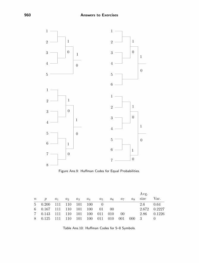
2.17: Figure Ans.9 shows Huffman codes for 5, 6, 7, and 8 symbols with equal proba-bilities. In the case where n is a power of 2, the codes are simply the fixed-sized ones.In other cases the codes are very close to fixed-size. This shows that symbols with equalprobabilities do not benefit from variable-size codes. (This is another way of saying thatrandom text cannot be compressed.) Table Ans.10 shows the codes, their average sizesand variances.
2.18: It increases exponentially from 2s to 2s+n = 2s × 2n.
2.19: The binary value of 127 is 01111111 and that of 128 is 10000000. Half the pixelsin each bitplane will therefore be 0 and the other half, 1. In the worst case, each bitplanewill be a checkerboard, i.e., will have many runs of size one. In such a case, each runrequires a 1-bit code, leading to one codebit per pixel per bitplane, or eight codebits perpixel for the entire image, resulting in no compression at all. In comparison, a Huffman
960 Answers to Exercises
1
2
3
4
5
6
7
8
1
1
1
0
0
0
1
2
3
4
5
6
1
1
0
0
1
2
3
4
5
6
7
1
1
1
0
0
0
1
2
3
4
5
1
1
0
0
Figure Ans.9: Huffman Codes for Equal Probabilities.
Avg.n p a1 a2 a3 a4 a5 a6 a7 a8 size Var.5 0.200 111 110 101 100 0 2.6 0.646 0.167 111 110 101 100 01 00 2.672 0.22277 0.143 111 110 101 100 011 010 00 2.86 0.12268 0.125 111 110 101 100 011 010 001 000 3 0
Table Ans.10: Huffman Codes for 5–8 Symbols.

Answers to Exercises 961
code for such an image requires just two codes (since there are just two pixel values) andthey can be one bit each. This leads to one codebit per pixel, or a compression factorof eight.
2.20: The two trees are shown in Figure 2.26c,d. The average code size for the binaryHuffman tree is
1×0.49 + 2×0.25 + 5×0.02 + 5×0.03 + 5×.04 + 5×0.04 + 3×0.12 = 2 bits/symbol,
and that of the ternary tree is
1×0.26 + 3×0.02 + 3×0.03 + 3×0.04 + 2×0.04 + 2×0.12 + 1×0.49 = 1.34 trits/symbol.
2.21: Figure Ans.11 shows how the loop continues until the heap shrinks to just onenode that is the single pointer 2. This indicates that the total frequency (which happensto be 100 in our example) is stored in A[2]. All other frequencies have been replacedby pointers. Figure Ans.12a shows the heaps generated during the loop.
2.22: The final result of the loop is
1 2 3 4 5 6 7 8 9 10 11 12 13 14[2 ] 100 2 2 3 4 5 3 4 6 5 7 6 7
from which it is easy to figure out the code lengths of all seven symbols. To find thelength of the code of symbol 14, e.g., we follow the pointers 7, 5, 3, 2 from A[14] to theroot. Four steps are necessary, so the code length is 4.
2.23: The code lengths for the seven symbols are 2, 2, 3, 3, 4, 3, and 4 bits. This canalso be verified from the Huffman code-tree of Figure Ans.12b. A set of codes derivedfrom this tree is shown in the following table:
Count: 25 20 13 17 9 11 5Code: 01 11 101 000 0011 100 0010Length: 2 2 3 3 4 3 4
2.24: A symbol with high frequency of occurrence should be assigned a shorter code.Therefore, it has to appear high in the tree. The requirement that at each level thefrequencies be sorted from left to right is artificial. In principle, it is not necessary, butit simplifies the process of updating the tree.
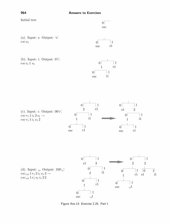
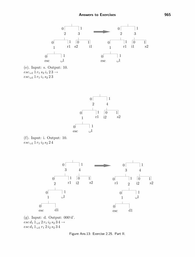
2.25: Figure Ans.13 shows the initial tree and how it is updated in the 11 steps (a)through (k). Notice how the esc symbol gets assigned different codes all the time, andhow the different symbols move about in the tree and change their codes. Code 10, e.g.,is the code of symbol “i” in steps (f) and (i), but is the code of “s” in steps (e) and (j).The code of a blank space is 011 in step (h), but 00 in step (k).
The final output is: “s0i00r100�1010000d011101000”. A total of 5×8 + 22 = 62bits. The compression ratio is thus 62/88 ≈ 0.7.

962 Answers to Exercises
1 2 3 4 5 6 7 8 9 10 11 12 13 14[7 11 6 8 9 ] 24 14 25 20 6 17 7 6 7
1 2 3 4 5 6 7 8 9 10 11 12 13 14[11 9 8 6 ] 24 14 25 20 6 17 7 6 7
1 2 3 4 5 6 7 8 9 10 11 12 13 14[11 9 8 6 ] 17+14 24 14 25 20 6 17 7 6 7
1 2 3 4 5 6 7 8 9 10 11 12 13 14[5 9 8 6 ] 31 24 5 25 20 6 5 7 6 7
1 2 3 4 5 6 7 8 9 10 11 12 13 14[9 6 8 5 ] 31 24 5 25 20 6 5 7 6 7
1 2 3 4 5 6 7 8 9 10 11 12 13 14[6 8 5 ] 31 24 5 25 20 6 5 7 6 7
1 2 3 4 5 6 7 8 9 10 11 12 13 14[6 8 5 ] 20+24 31 24 5 25 20 6 5 7 6 7
1 2 3 4 5 6 7 8 9 10 11 12 13 14[4 8 5 ] 44 31 4 5 25 4 6 5 7 6 7
1 2 3 4 5 6 7 8 9 10 11 12 13 14[8 5 4 ] 44 31 4 5 25 4 6 5 7 6 7
1 2 3 4 5 6 7 8 9 10 11 12 13 14[5 4 ] 44 31 4 5 25 4 6 5 7 6 7
1 2 3 4 5 6 7 8 9 10 11 12 13 14[5 4 ] 25+31 44 31 4 5 25 4 6 5 7 6 7
1 2 3 4 5 6 7 8 9 10 11 12 13 14[3 4 ] 56 44 3 4 5 3 4 6 5 7 6 7
1 2 3 4 5 6 7 8 9 10 11 12 13 14[4 3 ] 56 44 3 4 5 3 4 6 5 7 6 7
1 2 3 4 5 6 7 8 9 10 11 12 13 14[3 ] 56 44 3 4 5 3 4 6 5 7 6 7
1 2 3 4 5 6 7 8 9 10 11 12 13 14[3 ] 56+44 56 44 3 4 5 3 4 6 5 7 6 7
1 2 3 4 5 6 7 8 9 10 11 12 13 14[2 ] 100 2 2 3 4 5 3 4 6 5 7 6 7
Figure Ans.11: Sifting the Heap.

Answers to Exercises 963
5 9 11 13
17 20250
1
11
1
11
0
00
0
5
9 11
13 17 20 25
9
1113
17 2025
13 14
25 17 20
11
17 14
25 20
13
17 24
25 20
14
20 24
25
17
24 25
31
20
25 31
24
31 44
25
44
31
(a)
(b)
Figure Ans.12: (a) Heaps. (b) Huffman Code-Tree.
964 Answers to Exercises
Initial tree
(a). Input: s. Output: ‘s’.esc s1
(b). Input: i. Output: 0‘i’.esc i1 1 s1
esc0
1s1esc
0
s10
i1esc0
1
11
(c). Input: r. Output: 00‘r’.esc r1 1 i1 2 s1 →esc r1 1 i1 s1 2
s10
i10
1
12
1r1esc
0
1
s10
i10
1
12
1r1esc
0
1
(d). Input: �. Output: 100‘�’.esc �1 1 r1 2 i1 s1 3 →esc �1 1 r1 s1 i1 2 2
�1
s10
i10
1
13
1r1
0
2
esc0
1
1
�1
s1
0
i10
1
1
2
1r1
0
2
esc0
1
1
Figure Ans.13: Exercise 2.25. Part I.
Answers to Exercises 965
�1
s2
0
i10
1
1
3
1r1
0
2
esc0
1
1
s2
�1
0
i10
1
1
3
1r1
0
2
esc0
1
1
(e). Input: s. Output: 10.esc �1 1 r1 s2 i1 2 3 →esc �1 1 r1 i1 s2 2 3
s2
�1
0
i20
1
1
4
1r1
0
2
esc0
1
1
(f). Input: i. Output: 10.esc �1 1 r1 i2 s2 2 4
s2
�1
0
i20
1
1
4
1r1
0
3
0
2
1
d1esc0
1
s2
�1
0
i20
1
1
4
1r1
0
3
0
2
1
d1esc0
1
(g). Input: d. Output: 000‘d’.esc d1 1 �1 2 r1 i2 s2 3 4 →esc d1 1 �1 r1 2 i2 s2 3 4
Figure Ans.13: Exercise 2.25. Part II.

966 Answers to Exercises
s2�2
0
i20
1
1
4
1
r1
0
4
0
2
1
d1esc0
1
1
s2
�2
0
i20
1
1
4
1r1
0
4
0
3
1
d1esc0
1
1
(h). Input: �. Output: 011.esc d1 1 �2 r1 3 i2 s2 4 4 →esc d1 1 r1 �2 2 i2 s2 4 4
s2�2
0
i30
1
1
5
1
r1
0
4
0
2
1
d1esc0
1
1
s2�2
0
i30
1
1
5
1
r1
0
4
0
2
1
d1esc0
1
1
(i). Input: i. Output: 10.esc d1 1 r1 �2 2 i3 s2 4 5 →esc d1 1 r1 �2 2 s2 i3 4 5
Figure Ans.13: Exercise 2.25. Part III.

Answers to Exercises 967
s3�2
0
i30
1
1
6
1
r1
0
4
0
2
1
d1esc0
1
1
(j). Input: s. Output: 10.esc d1 1 r1 �2 2 s3 i3 4 6
s3�3
0
i30
1
1
6
1
r1
0
5
0
2
1
d1esc0
1
1
s3�3
0
i30
1
1
6
1
r1
0
5
0
2
1
d1esc0
1
1
(k). Input: �. Output: 00.esc d1 1 r1 �3 2 s3 i3 5 6 →esc d1 1 r1 2 �3 s3 i3 5 6
Figure Ans.13: Exercise 2.25. Part IV.

968 Answers to Exercises
2.26: A simple calculation shows that the average size of a token in Table 2.35 isabout nine bits. In stage 2, each 8-bit byte will be replaced, on average, by a 9-bittoken, resulting in an expansion factor of 9/8 = 1.125 or 12.5%.
2.27: The decompressor will interpret the input data as 111110 0110 11000 0. . . , whichis the string XRP. . . .
2.28: Because a typical fax machine scans lines that are about 8.2 inches wide (≈208 mm), so a blank scan line produces 1,664 consecutive white pels.
2.29: These codes are needed for cases such as example 4, where the run length is 64,128, or any length for which a make-up code has been assigned.
2.30: There may be fax machines (now or in the future) built for wider paper, so theGroup 3 code was designed to accommodate them.
2.31: Each scan line starts with a white pel, so when the decoder inputs the next codeit knows whether it is for a run of white or black pels. This is why the codes of Table 2.41have to satisfy the prefix property in each column but not between the columns.
2.32: Imagine a scan line where all runs have length one (strictly alternating pels).It’s easy to see that this case results in expansion. The code of a run length of one whitepel is 000111, and that of one black pel is 010. Two consecutive pels of different colorsare thus coded into 9 bits. Since the uncoded data requires just two bits (01 or 10),the compression ratio is 9/2 = 4.5 (the compressed stream is 4.5 times longer than theuncompressed one; a large expansion).
2.33: Figure Ans.14 shows the modes and the actual code generated from the twolines.
↑ ↑ ↑ ↑ ↑ ↑ ↑ ↑ ↑vertical mode horizontal mode pass vertical mode horizontal mode. . .
-1 0 3 white 4 black code +2 -2 4 white 7 black
↓ ↓ ↓ ↓ ↓ ↓ ↓ ↓ ↓ ↓ ↓010 1 001 1000 011 0001 000011 000010 001 1011 00011
Figure Ans.14: Two-Dimensional Coding Example.
2.34: Table Ans.15 shows the steps of encoding the string a2a2a2a2. Because of thehigh probability of a2 the low and high variables start at very different values andapproach each other slowly.
2.35: It can be written either as 0.1000. . . or 0.0111. . . .

Answers to Exercises 969
a2 0.0 + (1.0− 0.0)× 0.023162=0.0231620.0 + (1.0− 0.0)× 0.998162=0.998162
a2 0.023162 + .975× 0.023162=0.045744950.023162 + .975× 0.998162=0.99636995
a2 0.04574495 + 0.950625× 0.023162=0.067763226250.04574495 + 0.950625× 0.998162=0.99462270125
a2 0.06776322625 + 0.926859375× 0.023162=0.089231243093750.06776322625 + 0.926859375× 0.998162=0.99291913371875
Table Ans.15: Encoding the String a2a2a2a2.
2.36: In practice, the eof symbol has to be included in the original table of frequenciesand probabilities. This symbol is the last to be encoded, and the decoder stops when itdetects an eof.
2.37: The encoding steps are simple (see first example on page 114). We start withthe interval [0, 1). The first symbol a2 reduces the interval to [0.4, 0.9). The second one,to [0.6, 0.85), the third one to [0.7, 0.825) and the eof symbol, to [0.8125, 0.8250). Theapproximate binary values of the last interval are 0.1101000000 and 0.1101001100, sowe select the 7-bit number 1101000 as our code.
The probability of a2a2a2eof is (0.5)3×0.1 = 0.0125, but since − log2 0.0125 ≈ 6.322it follows that the practical minimum code size is 7 bits.
2.38: Perhaps the simplest way to do this is to compute a set of Huffman codes for thesymbols, using their probabilities. This converts each symbol to a binary string, so theinput stream can be encoded by the QM-coder. After the compressed stream is decodedby the QM-decoder, an extra step is needed, to convert the resulting binary strings backto the original symbols.
2.39: The results are shown in Tables Ans.16 and Ans.17. When all symbols are LPS,the output C always points at the bottom A(1 − Qe) of the upper (LPS) subinterval.When the symbols are MPS, the output always points at the bottom of the lower (MPS)subinterval, i.e., 0.
2.40: If the current input bit is an LPS, A is shrunk to Qe, which is always 0.5 or less,so A always has to be renormalized in such a case.
2.41: The results are shown in Tables Ans.18 and Ans.19 (compare with the answerto exercise 2.39).
2.42: The four decoding steps are as follows:Step 1: C = 0.981, A = 1, the dividing line is A(1−Qe) = 1(1− 0.1) = 0.9, so the LPSand MPS subintervals are [0, 0.9) and [0.9, 1). Since C points to the upper subinterval,an LPS is decoded. The new C is 0.981−1(1−0.1) = 0.081 and the new A is 1×0.1 = 0.1.Step 2: C = 0.081, A = 0.1, the dividing line is A(1−Qe) = 0.1(1− 0.1) = 0.09, so theLPS and MPS subintervals are [0, 0.09) and [0.09, 0.1), and an MPS is decoded. C isunchanged and the new A is 0.1(1− 0.1) = 0.09.

970 Answers to Exercises
Symbol C A
Initially 0 1s1 (LPS) 0 + 1(1− 0.5) = 0.5 1× 0.5 = 0.5s2 (LPS) 0.5 + 0.5(1− 0.5) = 0.75 0.5× 0.5 = 0.25s3 (LPS) 0.75 + 0.25(1− 0.5) = 0.875 0.25× 0.5 = 0.125s4 (LPS) 0.875 + 0.125(1− 0.5) = 0.9375 0.125× 0.5 = 0.0625
Table Ans.16: Encoding Four Symbols With Qe = 0.5.
Symbol C A
Initially 0 1s1 (MPS) 0 1× (1− 0.1) = 0.9s2 (MPS) 0 0.9× (1− 0.1) = 0.81s3 (MPS) 0 0.81× (1− 0.1) = 0.729s4 (MPS) 0 0.729× (1− 0.1) = 0.6561
Table Ans.17: Encoding Four Symbols With Qe = 0.1.
Symbol C A Renor. A Renor. C
Initially 0 1s1 (LPS) 0 + 1− 0.5 = 0.5 0.5 1 1s2 (LPS) 1 + 1− 0.5 = 1.5 0.5 1 3s3 (LPS) 3 + 1− 0.5 = 3.5 0.5 1 7s4 (LPS) 7 + 1− 0.5 = 6.5 0.5 1 13
Table Ans.18: Renormalization Added to Table Ans.16.
Symbol C A Renor. A Renor. C
Initially 0 1s1 (MPS) 0 1− 0.1 = 0.9s2 (MPS) 0 0.9− 0.1 = 0.8s3 (MPS) 0 0.8− 0.1 = 0.7 1.4 0s4 (MPS) 0 1.4− 0.1 = 1.3
Table Ans.19: Renormalization Added to Table Ans.17.

Answers to Exercises 971
Step 3: C = 0.081, A = 0.09, the dividing line is A(1−Qe) = 0.09(1− 0.1) = 0.0081, sothe LPS and MPS subintervals are [0, 0.0081) and [0.0081, 0.09), and an LPS is decoded.The new C is 0.081− 0.09(1− 0.1) = 0 and the new A is 0.09×0.1 = 0.009.Step 4: C = 0, A = 0.009, the dividing line is A(1 − Qe) = 0.009(1 − 0.1) = 0.00081,so the LPS and MPS subintervals are [0, 0.00081) and [0.00081, 0.009), and an MPS isdecoded. C is unchanged and the new A is 0.009(1− 0.1) = 0.00081.
2.43: In practice, an encoder may encode texts other than English, such as a foreignlanguage or the source code of a computer program. Acronyms, such as QED andabbreviations, such as qwerty, are also good examples. Even in English there are someexamples of a q not followed by a u, such as in this sentence. (The author has noticedthat science-fiction writers tend to use non-English sounding words, such as Qaal, toname characters in their works.)
2.44: The number of order-2 and order-3 contexts for an alphabet of size 28 = 256 is2562 = 65, 536 and 2563 = 16, 777, 216, respectively. The former is manageable, whereasthe latter is perhaps too big for a practical implementation, unless a sophisticated datastructure is used or unless the encoder gets rid of older data from time to time.
For a small alphabet, larger values of N can be used. For a 16-symbol alphabetthere are 164 = 65, 536 order-4 contexts and 166 = 16, 777, 216 order-6 contexts.
2.45: A practical example of a 16-symbol alphabet is a color or grayscale image with4-bit pixels. Each symbol is a pixel, and there are 16 different symbols.
2.46: An object file generated by a compiler or an assembler normally has severaldistinct parts including the machine instructions, symbol table, relocation bits, andconstants. Such parts may have different bit distributions.
2.47: The alphabet has to be extended, in such a case, to include one more symbol. Ifthe original alphabet consisted of all the possible 256 8-bit bytes, it should be extendedto 9-bit symbols, and should include 257 values.
2.48: Table Ans.20 shows the groups generated in both cases and makes it clear whythese particular probabilities were assigned.
2.49: The d is added to the order-0 contexts with frequency 1. The escape frequencyshould be incremented from 5 to 6, bringing the total frequencies from 19 up to 21. Theprobability assigned to the new d is therefore 1/21, and that assigned to the escape is6/21. All other probabilities are reduced from x/19 to x/21.
2.50: The new d would require switching from order 2 to order 0, sending two escapesthat take 1 and 1.32 bits. The d is now found in order-0 with probability 1/21, so itis encoded in 4.39 bits. The total number of bits required to encode the second d istherefore 1 + 1.32 + 4.39 = 6.71, still greater than 5.

972 Answers to Exercises
Context f pabc→x 10 10/11Esc 1 1/11
Context f pabc→ a1 1 1/20
→ a2 1 1/20→ a3 1 1/20→ a4 1 1/20→ a5 1 1/20→ a6 1 1/20→ a7 1 1/20→ a8 1 1/20→ a9 1 1/20→ a10 1 1/20
Esc 10 10/20Total 20
Table Ans.20: Stable vs. Variable Data.
2.51: The first three cases don’t change. They still code a symbol with 1, 1.32, and6.57 bits, which is less than the 8 bits required for a 256-symbol alphabet withoutcompression. Case 4 is different since the d is now encoded with a probability of 1/256,producing 8 instead of 4.8 bits. The total number of bits required to encode the d incase 4 is now 1 + 1.32 + 1.93 + 8 = 12.25.
2.52: The final trie is shown in Figure Ans.21.
a,4 s,6
s,2 a,2 s,3
s,2 a,2
n,1
n,1
n,1
i,2
i,1
i,1
s,1
s,1
s,1
i,1
i,1m,1
m,1
m,1
14. ‘a’
a,1
a,1
s,1
Figure Ans.21: Final Trie of assanissimassa.
2.53: This probability is, of course
1− Pe(bt+1 = 1|bt1) = 1− b + 1/2
a + b + 1=
a + 1/2a + b + 1
.

Answers to Exercises 973
2.54: For the first string the single bit has a suffix of 00, so the probability of leaf00 is Pe(1, 0) = 1/2. This is equal to the probability of string 0 without any suffix.For the second string each of the two zero bits has suffix 00, so the probability ofleaf 00 is Pe(2, 0) = 3/8 = 0.375. This is greater than the probability 0.25 of string00 without any suffix. Similarly, the probabilities of the remaining three strings arePe(3, 0) = 5/8 ≈ 0.625, Pe(4, 0) = 35/128 ≈ 0.273, and Pe(5, 0) = 63/256 ≈ 0.246.As the strings get longer, their probabilities get smaller but they are greater than theprobabilities without the suffix. Having a suffix of 00 thus increases the probability ofhaving strings of zeros following it.
2.55: The four trees are shown in Figure Ans.22a–d. The weighted probability thatthe next bit will be a zero given that three zeros have just been generated is 0.5. Theweighted probability to have two consecutive zeros given the suffix 000 is 0.375, higherthan the 0.25 without the suffix.
(a)
1
1
1
0 (1,0)
(1,0)
Pw=.5Pe=.5
.5
.5(1,0).5.5
(1,0).5.5
(b)
1
1
1
0 (2,0)
(2,0)
Pw=.375Pe=.375
.375
.375(2,0).375.375
(2,0).375.375
(c)
1
1
1
0
0
(1,0)
(1,0)
Pw=.5Pe=.5
.5
.5(1,0).5.5
(1,0).5.5
(d)
1 0
0 0
00
(0,1)
(0,2)
Pw=.3125Pe=.375
.5
.5
(0,1).5.5
(0,1).5.5
(0,1).5.5
(0,1).5.5
(0,1).5.5
000|0 000|00
000|11000|1
Figure Ans.22: Context Trees For 000|0, 000|00, 000|1, and 000|11.

974 Answers to Exercises
3.1: The size of the output stream is N [48−28P ] = N [48−25.2] = 22.8N . The size ofthe input stream is, as before, 40N . The compression factor is therefore 40/22.8 ≈ 1.75.
3.2: The list has up to 256 entries, each consisting of a byte and a count. A byteoccupies eight bits, but the counts depend on the size and content of the file beingcompressed. If the file has high redundancy, a few bytes may have large counts, close tothe length of the file, while other bytes may have very low counts. On the other hand,if the file is close to random, then each distinct byte has approximately the same count.
Thus, the first step in organizing the list is to reserve enough space for each “count”field to accommodate the maximum possible count. We denote the length of the file byL and find the positive integer k that satisfies 2k−1 < L ≤ 2k. Thus, L is a k-bit number.If k is not already a multiple of 8, we increase it to the next multiple of 8. We nowdenote k = 8m, and allocate m bytes to each “count” field.
Once the file has been input and processed and the list has been sorted, we examinethe largest count. It may be large and may occupy all m bytes, or it may be smaller.Assuming that the largest count occupies n bytes (where n ≤ m), we can store each ofthe other counts in n bytes.
When the list is written on the compressed file as the dictionary, its length s isfirst written in one byte. s is the number of distinct bytes in the original file. This isfollowed by n, followed by s groups, each with one of the distinct data bytes followed byan n-byte count. Notice that the value n should be fairly small and should fit in a singlebyte. If n does not fit in a single byte, then it is greater than 255, implying that thelargest count does not fit in 255 bytes, implying in turn a file whose length L is greaterthan 2255 ≈ 1076 bytes.
An alternative is to start with s, followed by n, followed by the s distinct databytes, followed by the n×s bytes of counts. The last part could also be in compressedform, because only a few largest counts will occupy all n bytes. Most counts may besmall and occupy just one or two bytes, which implies that many of the n×s count byteswill be zero, resulting in high redundancy and therefore good compression.
3.3: The straightforward answer is The decoder doesn’t know but it does not need toknow. The decoder simply reads tokens and uses each offset to locate a string of textwithout having to know whether the string was a first or a last match.
3.4: The next step matches the space and encodes the string �e.
sir�sid|�eastman�easily� ⇒ (4,1,e)sir�sid�e|astman�easily�te ⇒ (0,0,a)
and the next one matches nothing and encodes the a.
3.5: The first two characters CA at positions 17–18 are a repeat of the CA at positions9–10, so they will be encoded as a string of length 2 at offset 18− 10 = 8. The next twocharacters AC at positions 19–20 are a repeat of the string at positions 8–9, so they willbe encoded as a string of length 2 at offset 20− 9 = 11.
3.6: The decoder interprets the first 1 of the end marker as the start of a token. Thesecond 1 is interpreted as the prefix of a 7-bit offset. The next 7 bits are 0, and theyidentify the end marker as such, since a “normal” offset cannot be zero.

Answers to Exercises 975
Dictionary Token Dictionary Token15 �t (4, t) 21 �si (19,i)16 e (0, e) 22 c (0, c)17 as (8, s) 23 k (0, k)18 es (16,s) 24 �se (19,e)19 �s (4, s) 25 al (8, l)20 ea (4, a) 26 s(eof) (1, (eof))
Table Ans.23: Next 12 Encoding Steps in the LZ78 Example.
3.7: This is straightforward. The remaining steps are shown in Table Ans.23
3.8: Table Ans.24 shows the last three steps.
Hashp_src 3 chars index P Output Binary output
11 h�t 7 any→11 h 0110100012 �th 5 5→12 4,7 0000|0011|0000011116 ws ws 01110111|01110011
Table Ans.24: Last Steps of Encoding that thatch thaws.
The final compressed stream consists of 1 control word followed by 11 items (9 literalsand 2 copy items)0000010010000000|01110100|01101000|01100001|01110100|00100000|0000|0011|00000101|01100011|01101000|0000|0011|00000111|01110111|01110011.
3.9: An example is a compression utility for a personal computer that maintains allthe files (or groups of files) on the hard disk in compressed form, to save space. Such autility should be transparent to the user; it should automatically decompress a file everytime it is opened and automatically compress it when it is being closed. In order to betransparent, such a utility should be fast, with compression ratio being only a secondaryfeature.
3.10: Table Ans.25 summarizes the steps. The output emitted by the encoder is97 (a), 108 (l), 102 (f), 32 (�), 101 (e), 97 (a), 116 (t), 115 (s), 32 (�), 256 (al), 102(f), 265 (alf), 97 (a),and the following new entries are added to the dictionary(256: al), (257: lf), (258: f�), (259: �e), (260: ea), (261: at), (262: ts),(263: s�), (264: �a), (265: alf), (266: fa), (267: alfa).
3.11: The encoder inputs the first a into I, searches and finds a in the dictionary.It inputs the next a but finds that Ix, which is now aa, is not in the dictionary. Theencoder thus adds string aa to the dictionary as entry 256 and outputs the token 97 (a).Variable I is initialized to the second a. The third a is input, so Ix is the string aa, whichis now in the dictionary. I becomes this string, and the fourth a is input. Ix is now aaa

976 Answers to Exercises
in new in newI dict? entry output I dict? entry output
a Y s� N 263-s� 115 (s)al N 256-al 97 (a) � Yl Y �a N 264-�a 32 (�)lf N 257-lf 108 (l) a Yf Y al Yf� N 258-f� 102 (f) alf N 265-alf 256 (al)� Y f Y�e N 259-�e 32 (w) fa N 266-fa 102 (f)e Y a Yea N 260-ea 101 (e) al Ya Y alf Yat N 261-at 97 (a) alfa N 267-alfa 265 (alf)t Y a Yts N 262-ts 116 (t) a,eof N 97 (a)s Y
Table Ans.25: LZW Encoding of “alf eats alfalfa”.
which is not in the dictionary. The encoder thus adds string aaa to the dictionary asentry 257 and outputs 256 (aa). I is initialized to the fourth a. Continuing this processis straightforward.
The result is that strings aa, aaa, aaaa,. . . are added to the dictionary as entries256, 257, 258,. . . , and the output is
97 (a), 256 (aa), 257 (aaa), 258 (aaaa),. . .
The output consists of pointers pointing to longer and longer strings of as. The first kpointers thus point at strings whose total length is 1 + 2 + · · ·+ k = (k + k2)/2.
Assuming an input stream that consists of one million as, we can find the size ofthe compressed output stream by solving the quadratic equation (k + k2)/2 = 1000000for the unknown k. The solution is k ≈ 1414. The original, 8-million bit input is thuscompressed into 1414 pointers, each at least 9-bit (and in practice, probably 16-bit) long.The compression factor is thus either 8M/(1414×9) ≈ 628.6 or 8M/(1414×16) ≈ 353.6.
This is an impressive result but such input streams are rare (notice that this par-ticular input can best be compressed by generating an output stream containing just“1000000 a”, and without using LZW).
3.12: We simply follow the decoding steps described in the text. The results are:1. Input 97. This is in the dictionary so set I=a and output a. String ax needs to besaved in the dictionary but x is still unknown.2. Input 108. This is in the dictionary so set J=l and output l. Save al in entry 256.Set I=l.3. Input 102. This is in the dictionary so set J=f and output f. Save lf in entry 257.Set I=f.
Answers to Exercises 977
4. Input 32. This is in the dictionary so set J=� and output �. Save f� in entry 258.Set I=�.5. Input 101. This is in the dictionary so set J=e and output e. Save �e in entry 259.Set I=e.6. Input 97. This is in the dictionary so set J=a and output a. Save ea in entry 260.Set I=a.7. Input 116. This is in the dictionary so set J=t and output t. Save at in entry 261.Set I=t.8. Input 115. This is in the dictionary so set J=s and output s. Save ts in entry 262.Set I=t.9. Input 32. This is in the dictionary so set J=� and output �. Save s� in entry 263.Set I=�.10. Input 256. This is in the dictionary so set J=al and output al. Save �a in entry264. Set I=al.11. Input 102. This is in the dictionary so set J=f and output f. Save alf in entry265. Set I=f.12. Input 265. This has just been saved in the dictionary so set J=alf and output alf.Save fa in dictionary entry 266. Set I=alf.13. Input 97. This is in the dictionary so set J=a and output a. Save alfa in entry 267(even though it will never be used). Set I=a.14. Read eof. Stop.
3.13: We assume that the dictionary is initialized to just the two entries (1: a) and(2: b). The encoder outputs
1 (a), 2 (b), 3 (ab), 5(aba), 4(ba), 7 (bab), 6 (abab), 9 (ababa), 8 (baba),. . .
and adds the new entries (3: ab), (4: ba), (5: aba), (6: abab), (7: bab), (8: baba), (9:ababa), (10: ababab), (11: babab),. . . to the dictionary. This regular behavior can beanalyzed and the kth output pointer and dictionary entry predicted, but the effort isprobably not worth it.
3.14: The answer to exercise 3.11 shows the relation between the size of the compressedfile and the size of the largest dictionary string for the “worst case” situation (input thatcreates the longest strings). For a 1 Mbyte input stream, there will be 1,414 strings inthe dictionary, the largest of which is 1,414 symbols long.
3.15: This is straightforward (Table Ans.26) but not very efficient since only one two-symbol dictionary phrase is used.
3.16: Table Ans.27 shows all the steps. In spite of the short input, the result is quitegood (13 codes to compress 18-symbols) because the input contains concentrations of asand bs.
3.17: 1. The encoder starts by shifting the first two symbols xy to the search buffer,outputting them as literals and initializing all locations of the index table to the nullpointer.

978 Answers to Exercises
Add toStep Input Output S dict. S’
swiss�miss
1 s 115 s — s2 w 119 w 256-sw w3 i 105 i 257-wi i4 s 115 s 258-is s5 s 115 s 259-ss s6 - 32 � 260-s� �7 m 109 m 261-�m m8 is 258 is 262-mis is9 s 115 s 263-iss s
Table Ans.26: LZMW Compression of “swiss miss”.
Add toStep Input Output S dict. S’
yabbadabbadabbadoo
1 y 121 y — y2 a 97 a 256-ya a3 b 98 b 257-ab b4 b 98 b 258-bb b5 a 97 a 259-ba a6 d 100 a 260-ad a7 ab 257 ab 261-dab ab8 ba 259 ba 262-abba ba9 dab 261 dab 263-badab dab10 ba 259 ba 264-dabba ba11 d 100 d 265-bad d12 o 111 o 266-do o13 o 111 o 267-o o
Table Ans.27: LZMW Compression of “yabbadabbadabbadoo”.
2. The current symbol is a (the first a) and the context is xy. It is hashed to, say, 5,but location 5 of the index table contains a null pointer, so P is null. Location 5 is set topoint to the first a, which is then output as a literal. The data in the encoder’s bufferis shifted to the left.3. The current symbol is the second a and the context is ya. It is hashed to, say, 1, butlocation 1 of the index table contains a null pointer, so P is null. Location 1 is set topoint to the second a, which is then output as a literal. The data in the encoder’s bufferis shifted to the left.4. The current symbol is the third a and the context is aa. It is hashed to, say, 2, butlocation 2 of the index table contains a null pointer, so P is null. Location 2 is set topoint to the third a, which is then output as a literal. The data in the encoder’s bufferis shifted to the left.

Answers to Exercises 979
5. The current symbol is the fourth a and the context is aa. We know from step 4 thatit is hashed to 2, and location 2 of the index table points to the third a. Location 2 isset to point to the fourth a, and the encoder tries to match the string starting with thethird a to the string starting with the fourth a. Assuming that the look-ahead buffer isfull of as, the match length L will be the size of that buffer. The encoded value of Lwill be written to the compressed stream, and the data in the buffer shifted L positionsto the left.6. If the original input stream is long, more a’s will be shifted into the look-ahead buffer,and this step will also result in a match of length L. If only n as remain in the inputstream, they will be matched, and the encoded value of n output.
The compressed stream will consist of the three literals x, y, and a, followed by(perhaps several values of) L, and possibly ending with a smaller value.
3.18: T percent of the compressed stream is made up of literals, some appearingconsecutively (and thus getting the flag “1” for two literals, half a bit per literal) andothers with a match length following them (and thus getting the flag “01”, one bit forthe literal). We assume that two thirds of the literals appear consecutively and one thirdare followed by match lengths. The total number of flag bits created for literals is thus
23T × 0.5 +
13T × 1.
A similar argument for the match lengths yields
23(1− T )× 2 +
13(1− T )× 1
for the total number of the flag bits. We now write the equation
23T × 0.5 +
13T × 1 +
23(1− T )× 2 +
13(1− T )× 1 = 1,
which is solved to yield T = 2/3. This means that if two thirds of the items in thecompressed stream are literals, there would be 1 flag bit per item on the average. Moreliterals would result in fewer flag bits.
3.19: The first three 1’s indicate six literals. The following 01 indicates a literal (b)followed by a match length (of 3). The 10 is the code of match length 3, and the last 1indicates two more literals (x and y).
4.1: An image with no redundancy is not always random. The definition of redundancy(Section 2.1) tells us that an image where each color appears with the same frequencyhas no redundancy (statistically) yet it is not necessarily random and may even beinteresting and/or useful.

980 Answers to Exercises
5 10 15 20 25 30
5
10
15
20
25
30
5 10 15 20 25 30
5
10
15
20
25
30
5 10 15 20 25 30
5
10
15
20
25
30
5 10 15 20 25 30
5
10
15
20
25
30
a b
cov(a) cov(b)
Figure Ans.28: Covariance Matrices of Correlated and Decorrelated Values.
a=rand(32); b=inv(a);figure(1), imagesc(a), colormap(gray); axis squarefigure(2), imagesc(b), colormap(gray); axis squarefigure(3), imagesc(cov(a)), colormap(gray); axis squarefigure(4), imagesc(cov(b)), colormap(gray); axis square
Code for Figure Ans.28.
4.2: Figure Ans.28 shows two 32×32 matrices. The first one, a, with random (andtherefore decorrelated) values and the second one, b, is its inverse (and therefore withcorrelated values). Their covariance matrices are also shown and it is obvious that matrixcov(a) is close to diagonal, whereas matrix cov(b) is far from diagonal. The Matlab codefor this figure is also listed.

Answers to Exercises 981
4.3: The results are shown in Table Ans.29 together with the Matlab code used tocalculate it.
43210 Gray 43210 Gray 43210 Gray 43210 Gray00000 00000 01000 01100 10000 11000 11000 1010000001 00001 01001 01101 10001 11001 11001 1010100010 00011 01010 01111 10010 11011 11010 1011100011 00010 01011 01110 10011 11010 11011 1011000100 00110 01100 01010 10100 11110 11100 1001000101 00111 01101 01011 10101 11111 11101 1001100110 00101 01110 01001 10110 11101 11110 1000100111 00100 01111 01000 10111 11100 11111 10000
Table Ans.29: First 32 Binary and Gray Codes.
a=linspace(0,31,32); b=bitshift(a,-1);b=bitxor(a,b); dec2bin(b)
Code for Table Ans.29.
4.4: One feature is the regular way in which each of the five code bits alternatesperiodically between 0 and 1. It is easy to write a program that will set all five bits to 0,will flip the rightmost bit after two codes have been calculated, and will flip any of theother four code bits in the middle of the period of its immediate neighbor on the right.Another feature is the fact that the second half of the table is a mirror image of the firsthalf, but with the most significant bit set to one. After the first half of the table hasbeen computed, using any method, this symmetry can be used to quickly calculate thesecond half.
4.5: Figure Ans.30 is an angular code wheel representation of the 4-bit and 6-bit RGCcodes (part a) and the 4-bit and 6-bit binary codes (part b). The individual bitplanesare shown as rings, with the most significant bits as the innermost ring. It is easy tosee that the maximum angular frequency of the RGC is half that of the binary code andthat the first and last codes also differ by just one bit.
4.6: If pixel values are in the range [0, 255], a difference (Pi −Qi) can be at most 255.The worst case is where all the differences are 255. It is easy to see that such a caseyields an RMSE of 255.
4.7: The code of Figure 4.15 yields the coordinates of the rotated points
(7.071, 0), (9.19, 0.7071), (17.9, 0.78), (33.9, 1.41), (43.13,−2.12)
(notice how all the y coordinates are small numbers) and shows that the cross-correlationdrops from 1729.72 before the rotation to −23.0846 after it. A significant reduction!

982 Answers to Exercises
(a)
(b)
Figure Ans.30: Angular Code Wheels of RGC and Binary Codes.
4.8: Figure Ans.31 shows the 64 basis images and the Matlab code to calculate anddisplay them. Each basis image is an 8× 8 matrix.
4.9: A4 is the 4×4 matrix
A4 =
⎛⎜⎝
h0(0/4) h0(1/4) h0(2/4) h0(3/4)h1(0/4) h1(1/4) h1(2/4) h1(3/4)h2(0/4) h2(1/4) h2(2/4) h2(3/4)h3(0/4) h3(1/4) h3(2/4) h3(3/4)
⎞⎟⎠ =
1√4
⎛⎜⎝
1 1 1 11 1 −1 −1√2 −√2 0 0
0 0√
2 −√2
⎞⎟⎠ .
Similarly, A8 is the matrix
A8 =1√8
⎛⎜⎜⎜⎜⎜⎜⎜⎜⎜⎝
1 1 1 1 1 1 1 11 1 1 1 −1 −1 −1 −1√2√
2 −√2 −√2 0 0 0 00 0 0 0
√2√
2 −√2 −√22 −2 0 0 0 0 0 00 0 2 −2 0 0 0 00 0 0 0 2 −2 0 00 0 0 0 0 0 2 −2
⎞⎟⎟⎟⎟⎟⎟⎟⎟⎟⎠
.

Answers to Exercises 983
M=3; N=2^M; H=[1 1; 1 -1]/sqrt(2);for m=1:(M-1) % recursionH=[H H; H -H]/sqrt(2);
endA=H’;map=[1 5 7 3 4 8 6 2]; % 1:Nfor n=1:N, B(:,n)=A(:,map(n)); end;A=B;sc=1/(max(abs(A(:))).^2); % scale factorfor row=1:Nfor col=1:NBI=A(:,row)*A(:,col).’; % tensor productsubplot(N,N,(row-1)*N+col)oe=round(BI*sc); % results in -1, +1imagesc(oe), colormap([1 1 1; .5 .5 .5; 0 0 0])drawnow
endend
Figure Ans.31: The 8×8 WHT Basis Images and Matlab Code.

984 Answers to Exercises
4.10: The average of vector w(i) is zero, so Equation (4.12) yields
(W·WT
)jj
=k∑
i=1
w(i)j w
(i)j =
k∑i=1
(w
(i)j − 0
)2
=k∑
i=1
(c(j)i − 0
)2
= k Variance(c(j)).
4.11: The Mathematica code of Figure 4.21 produces the eight coefficients 140, −71, 0,−7, 0, −2, 0, and 0. We now quantize this set coarsely by clearing the last two nonzeroweights −7 and −2, When the IDCT is applied to the sequence 140, −71, 0, 0, 0, 0, 0,0, it produces 15, 20, 30, 43, 56, 69, 79, and 84. These are not identical to the originalvalues, but the maximum difference is only 4; an excellent result considering that onlytwo of the eight DCT coefficients are nonzero.
4.12: The eight values in the top row are very similar (the differences between themare either 2 or 3). Each of the other rows is obtained as a right-circular shift of thepreceding row.
4.13: It is obvious that such a block can be represented as a linear combination of thepatterns in the leftmost column of Figure 4.39. The actual calculation yields the eightweights 4, 0.72, 0, 0.85, 0, 1.27, 0, and 3.62 for the patterns of this column. The other56 weights are zero or very close to zero.
4.14: The arguments of the cosine functions used by the DCT are of the form (2x +1)iπ/16, where i and x are integers in the range [0, 7]. Such an argument can be writtenin the form nπ/16, where n is an integer in the range [0, 15×7]. Since the cosine functionis periodic, it satisfies cos(32π/16) = cos(0π/16), cos(33π/16) = cos(π/16), and so on.As a result, only the 32 values cos(nπ/16) for n = 0, 1, 2, . . . , 31 are needed. The authoris indebted to V. Saravanan for pointing out this feature of the DCT.
4.15: Figure 4.52 shows the results (that resemble Figure 4.39) and the Matlab code.Notice that the same code can also be used to calculate and display the DCT basisimages.
4.16: First figure out the zigzag path manually, then record it in an array zz ofstructures, where each structure contains a pair of coordinates for the path as shown,e.g., in Figure Ans.32.
(0,0) (0,1) (1,0) (2,0) (1,1) (0,2) (0,3) (1,2)(2,1) (3,0) (4,0) (3,1) (2,2) (1,3) (0,4) (0,5)(1,4) (2,3) (3,2) (4,1) (5,0) (6,0) (5,1) (4,2)(3,3) (2,4) (1,5) (0,6) (0,7) (1,6) (2,5) (3,4)(4,3) (5,2) (6,1) (7,0) (7,1) (6,2) (5,3) (4,4)(3,5) (2,6) (1,7) (2,7) (3,6) (4,5) (5,4) (6,3)(7,2) (7,3) (6,4) (5,5) (4,6) (3,7) (4,7) (5,6)(6,5) (7,4) (7,5) (6,6) (5,7) (6,7) (7,6) (7,7)
Figure Ans.32: Coordinates for the Zigzag Path.

Answers to Exercises 985
If the two components of a structure are zz.r and zz.c, then the zigzag traversalcan be done by a loop of the form :
for (i=0; i<64; i++){row:=zz[i].r; col:=zz[i].c...data_unit[row][col]...}
4.17: The third DC difference, 5, is located in row 3 column 5, so it is encoded as1110|101.
4.18: Thirteen consecutive zeros precede this coefficient, so Z = 13. The coefficientitself is found in Table 4.63 in row 1, column 0, so R = 1 and C = 0. Assuming thatthe Huffman code in position (R,Z) = (1, 13) of Table 4.66 is 1110101, the final codeemitted for 1 is 1110101|0.
4.19: This is shown by multiplying the largest four n-bit number, 11 . . . 1︸ ︷︷ ︸n
by 4, which
is easily done by shifting it 2 positions to the left. The result is the n + 2-bit number11 . . . 1︸ ︷︷ ︸
n
00.
4.20: They make for a more natural progressive growth of the image. They make iteasier for a person watching the image develop on the screen to decide if and when tostop the decoding process and accept or discard the image.
4.21: The only specification that depends on the particular bits assigned to the twocolors is Equation (4.25). All the other parts of JBIG are independent of the bit assign-ment.
4.22: For the 16-bit template of Figure 4.97a the relative coordinates are
A1 = (3,−1), A2 = (−3,−1), A3 = (2,−2), A4 = (−2,−2).
For the 13-bit template of Figure 4.97b the relative coordinates of A1 are (3,−1). Forthe 10-bit templates of Figure 4.97c,d the relative coordinates of A1 are (2,−1).
4.23: Transposing S and T produces better compression in cases where the text runsvertically.
4.24: Going back to step 1 we have the same points participate in the partition foreach codebook entry (this happens because our points are concentrated in four distinctregions, but in general a partition P
(k)i may consist of different image blocks in each
iteration k). The distortions calculated in step 2 are summarized in Table Ans.34. Theaverage distortion D
(1)i is
D(1) = (277+277+277+277+50+50+200+117+37+117+162+117)/12 = 163.17,
much smaller than the original 603.33. If step 3 indicates no convergence, more iterationsshould follow (Exercise 4.25), reducing the average distortion and improving the valuesof the four codebook entries.

986 Answers to Exercises
B1 B2
B3 B4
B5 C2
C1
C3
C4
B6
B7
B8
B9
B10
B11
B12
×
× ×
×
20
20
40
40
60
60
80
80
100
100
120
120
140
140
160
160
180
180
200
200
220
220
240
240
Figure Ans.33: Twelve Points and Four Codebook Entries C(1)i .
I: (46− 32)2 + (41− 32)2 = 277, (46− 60)2 + (41− 32)2 = 277,(46− 32)2 + (41− 50)2 = 277, (46− 60)2 + (41− 50)2 = 277,
II: (65− 60)2 + (145− 150)2 = 50, (65− 70)2 + (145− 140)2 = 50,III: (210− 200)2 + (200− 210)2 = 200,IV: (206− 200)2 + (41− 32)2 = 117, (206− 200)2 + (41− 40)2 = 37,
(206− 200)2 + (41− 50)2 = 117, (206− 215)2 + (41− 50)2 = 162,(206− 215)2 + (41− 35)2 = 117.
Table Ans.34: Twelve Distortions for k = 1.

Answers to Exercises 987
4.25: Each new codebook entry C(k)i is calculated, in step 4 of iteration k, as the
average of the block images comprising partition P(k−1)i . In our example the image
blocks (points) are concentrated in four separate regions, so the partitions calculatedfor iteration k = 1 are the same as those for k = 0. Another iteration, for k = 2,will therefore compute the same partitions in its step 1 yielding, in step 3, an averagedistortion D(2) that equals D(1). Step 3 will therefore indicate convergence.
4.26: It is 4−8 ≈ 0.000015 the area of the entire space.
4.27: Monitor the compression ratio and delete the dictionary and start afresh eachtime compression performance drops below a certain threshold.
4.28: Step 4: Point (2, 0) is popped out of the GPP. The pixel value at this position is7. The best match for this point is with the dictionary entry containing 7. The encoderoutputs the pointer 7. The match does not have any concave corners, so we push thepoint on the right of the matched block, (2, 1), and the point below it, (3, 0), into theGPP. The GPP now contains points (2, 1), (3, 0), (0, 2), and (1, 1). The dictionary is
updated by appending to it (at location 18) the block 47 .
Step 5: Point (1, 1) is popped out of the GPP. The pixel value at this position is5. The best match for this point is with the dictionary entry containing 5. The encoderoutputs the pointer 5. The match does not have any concave corners, so we push thepoint to the right of the matched block, (1, 2), and the point below it, (2, 1), into theGPP. The GPP contains points (1, 2), (2, 1), (3, 0), and (0, 2). The dictionary is updated
by appending to it (at locations 19, 20) the two blocks 25 and 4 5 .
4.29: It may simply be too long. When compressing text, each symbol is normally 1-byte long (two bytes in Unicode). However, images with 24-bit pixels are very common,and a 16-pixel block in such an image is 48-bytes long.
4.30: If the encoder uses a (2, 1, k) general unary code, then the value of k should alsobe included in the header.
4.31: The mean and standard deviation are p = 115 and σ = 77.93, respectively. Thecounts become n+ = n− = 8, and Equations (4.33) are solved to yield p+ = 193 andp− = 37. The original block is compressed to the 16 bits
⎛⎜⎝
1 0 1 11 0 0 11 1 0 10 0 0 0
⎞⎟⎠ ,
and the two 8-bit values 37 and 193.
4.32: Table Ans.35 summarizes the results. Notice how a 1-pixel with a context of 00is assigned high probability after being seen 3 times.

988 Answers to Exercises
# Pixel Context Counts Probability New counts
5 0 10=2 1,1 1/2 2,16 1 00=0 1,3 3/4 1,47 0 11=3 1,1 1/2 2,18 1 10=2 2,1 1/3 2,2
Table Ans.35: Counts and Probabilities for Next Four Pixels.
4.33: Such a thing is possible for the encoder but not for the decoder. A compressionmethod using “future” pixels in the context is useless because its output would beimpossible to decompress.
4.34: The model used by FELICS to predict the current pixel is a second-order Markovmodel. In such a model the value of the current data item depends on just two of itspast neighbors, not necessarily the two immediate ones.
4.35: The two previously seen neighbors of P=8 are A=1 and B=11. P is thus in thecentral region, where all codes start with a zero, and L=1, H=11. The computationsare straightforward:
k = �log2(11− 1 + 1)� = 3, a = 23+1 − 11 = 5, b = 2(11− 23) = 6.
Table Ans.36 lists the five 3-bit codes and six 4-bit codes for the central region.The code for 8 is thus 0|111.
The two previously seen neighbors of P=7 are A=2 and B=5. P is thus in the rightouter region, where all codes start with 11, and L=2, H=7. We are looking for the codeof 7− 5 = 2. Choosing m = 1 yields, from Table 4.120, the code 11|01.
The two previously seen neighbors of P=0 are A=3 and B=5. P is thus in the leftouter region, where all codes start with 10, and L=3, H=5. We are looking for the codeof 3− 0 = 3. Choosing m = 1 yields, from Table 4.120, the code 10|100.
Pixel Region PixelP code code
1 0 00002 0 00103 0 01004 0 0115 0 1006 0 1017 0 1108 0 1119 0 0001
10 0 001111 0 0101
Table Ans.36: The Codes for a Central Region.

Answers to Exercises 989
4.36: Because the decoder has to resolve ties in the same way as the encoder.
4.37: The weights have to add up to 1 because this results in a weighted sum whosevalue is in the same range as the values of the pixels. If pixel values are, for example,in the range [0, 15] and the weights add up to 2, a prediction may result in values of upto 30.
4.38: Each of the three weights 0.0039, −0.0351, and 0.3164 is used twice. The sumof the weights is therefore 0.5704, and the result of dividing each weight by this sumis 0.0068, −0.0615, and 0.5547. It is easy to verify that the sum of the renormalizedweights 2(0.0068− 0.0615 + 0.5547) equals 1.
4.39: An archive of static images is an example where this approach is practical. NASAhas a large archive of images taken by various satellites. They should be kept highlycompressed, but they never change, so each image has to be compressed only once. Aslow encoder is therefore acceptable but a fast decoder is certainly handy. Anotherexample is an art collection. Many museums have already scanned and digitized theircollections of paintings, and those are also static.
4.40: Such a polynomial depends on three coefficients b, c, and d that can be consid-ered three-dimensional points, and any three points are on the same plane.
4.41: This is straightforward
P(2/3) =(0,−9)(2/3)3 + (−4.5, 13.5)(2/3)2 + (4.5,−3.5)(2/3)=(0,−8/3) + (−2, 6) + (3,−7/3)=(1, 1) = P3.
4.42: We use the relations sin 30◦ = cos 60◦ = .5 and the approximation cos 30◦ =sin 60◦ ≈ .866. The four points are P1 = (1, 0), P2 = (cos 30◦, sin 30◦) = (.866, .5),P3 = (.5, .866), and P4 = (0, 1). The relation A = N ·P becomes⎛
⎜⎝abcd
⎞⎟⎠ = A = N ·P =
⎛⎜⎝−4.5 13.5 −13.5 4.59.0 −22.5 18 −4.5−5.5 9.0 −4.5 1.01.0 0 0 0
⎞⎟⎠⎛⎜⎝
(1, 0)(.866, .5)(.5, .866)
(0, 1)
⎞⎟⎠
and the solutions are
a = −4.5(1, 0) + 13.5(.866, .5)− 13.5(.5, .866) + 4.5(0, 1) = (.441,−.441),b = 19(1, 0)− 22.5(.866, .5) + 18(.5, .866)− 4.5(0, 1) = (−1.485,−0.162),c = −5.5(1, 0) + 9(.866, .5)− 4.5(.5, .866) + 1(0, 1) = (0.044, 1.603),d = 1(1, 0)− 0(.866, .5) + 0(.5, .866)− 0(0, 1) = (1, 0).
Thus, the PC is P(t) = (.441,−.441)t3 + (−1.485,−0.162)t2 + (0.044, 1.603)t + (1, 0).The midpoint is P(.5) = (.7058, .7058), only 0.2% away from the midpoint of the arc,which is at (cos 45◦, sin 45◦) ≈ (.7071, .7071).

990 Answers to Exercises
4.43: The new equations are easy enough to set up. Using Mathematica, they are alsoeasy to solve. The following code
Solve[{d==p1,a al^3+b al^2+c al+d==p2,a be^3+b be^2+c be+d==p3,a+b+c+d==p4},{a,b,c,d}];ExpandAll[Simplify[%]]
(where al and be stand for α and β, respectively) produces the (messy) solutions
a = −P1
αβ+
P2
−α2 + α3 + αβ − α2β+
P3
αβ − β2 − αβ2 + β3+
P4
1− α− β + αβ,
b = P1
(−α + α3 + β − α3β − β3 + αβ3)/γ + P2
(−β + β3)/γ
+ P3
(α− α3
)/γ + P4
(α3β − αβ3
)/γ,
c = −P1
(1 +
1α
+1β
)+
βP2
−α2 + α3 + αβ − α2β
+αP3
αβ − β2 − αβ2 + β3+
αβP4
1− α− β + αβ,
d = P1,
where γ = (−1 + α)α(−1 + β)β(−α + β).
From here, the basis matrix immediately follows
⎛⎜⎜⎜⎜⎝
− 1αβ
1−α2+α3αβ−α2β
1αβ−β2−αβ2+β3
11−α−β+αβ
−α+α3+β−α3β−β3+αβ3
γ−β+β3
γα−α3
γα3β−αβ3
γ
−(1 + 1
α + 1β
)β
−α2+α3+αβ−α2βα
αβ−β2−αβ2+β3αβ
1−α−β+αβ
1 0 0 0
⎞⎟⎟⎟⎟⎠ .
A direct check, again using Mathematica, for α = 1/3 and β = 2/3, reduces this matrixto matrix N of Equation (4.44).
4.44: The missing points will have to be estimated by interpolation or extrapolationfrom the known points before our method can be applied. Obviously, the fewer pointsare known, the worse the final interpolation. Note that 16 points are necessary, becausea bicubic polynomial has 16 coefficients.
4.45: Figure Ans.37a shows a diamond-shaped grid of 16 equally-spaced points. Theeight points with negative weights are shown in black. Figure Ans.37b shows a cut(labeled xx) through four points in this surface. The cut is a curve that passes throughpour data points. It is easy to see that when the two exterior (black) points are raised,the center of the curve (and, as a result, the center of the surface) gets lowered. It is

Answers to Exercises 991
now clear that points with negative weights push the center of the surface in a directionopposite that of the points.
Figure Ans.37c is a more detailed example that also shows why the four cornerpoints should have positive weights. It shows a simple symmetric surface patch thatinterpolates the 16 points
P00 = (0, 0, 0), P10 = (1, 0, 1), P20 = (2, 0, 1), P30 = (3, 0, 0),P01 = (0, 1, 1), P11 = (1, 1, 2), P21 = (2, 1, 2), P31 = (3, 1, 1),P02 = (0, 2, 1), P12 = (1, 2, 2), P22 = (2, 2, 2), P32 = (3, 2, 1),P03 = (0, 3, 0), P13 = (1, 3, 1), P23 = (2, 3, 1), P33 = (3, 3, 0).
We first raise the eight boundary points from z = 1 to z = 1.5. Figure Ans.37d showshow the center point P(.5, .5) gets lowered from (1.5, 1.5, 2.25) to (1.5, 1.5, 2.10938). Wenext return those points to their original positions and instead raise the four cornerpoints from z = 0 to z = 1. Figure Ans.37e shows how this raises the center point from(1.5, 1.5, 2.25) to (1.5, 1.5, 2.26563).
4.46: The decoder knows this pixel since it knows the value of average μ[i − 1, j] =0.5(I[2i− 2, 2j] + I[2i− 1, 2j + 1]) and since it has already decoded pixel I[2i− 2, 2j]
4.47: The decoder knows how to do this because when the decoder inputs the 5, itknows that the difference between p (the pixel being decoded) and the reference pixelstarts at position 6 (counting from the left). Since bit 6 of the reference pixel is 0, thatof p must be 1.
4.48: Yes, but compression would suffer. One way to apply this method is to separateeach byte into two 4-bit pixels and encode each pixel separately. This approach is badsince the prefix and suffix of a 4-bit pixel may often consist of more than four bits.Another approach is to ignore the fact that a byte contains two pixels, and use themethod as originally described. This may still compress the image, but is not veryefficient, as the following example illustrates.
Example: The two bytes 1100|1101 and 1110|1111 represent four pixels, each dif-fering from its immediate neighbor by its least-significant bit. The four pixels thereforehave similar colors (or grayscales). Comparing consecutive pixels results in prefixes of 3or 2, but comparing the two bytes produces the prefix 2.
4.49: The weights add up to 1 because this produces a value X in the same range asA, B, and C. If the weights were, for instance, 1, 100, and 1, X would have much biggervalues than any of the three pixels.
4.50: The four vectors are
a = (90, 95, 100, 80, 90, 85),
b(1) = (100, 90, 95, 102, 80, 90),
b(2) = (101, 128, 108, 100, 90, 95),
b(3) = (128, 108, 110, 90, 95, 100),

992 Answers to Exercises
(a)
x
x
(b)
1
23
0
12
30
0
1
2
0
1
23
0
12
3
2
0
1
0
1
2
3
0
1
23
1
2
(c) (d) (e)Figure Ans.37: An Interpolating Bicubic Surface Patch.
Clear[Nh,p,pnts,U,W];
p00={0,0,0}; p10={1,0,1}; p20={2,0,1}; p30={3,0,0};
p01={0,1,1}; p11={1,1,2}; p21={2,1,2}; p31={3,1,1};
p02={0,2,1}; p12={1,2,2}; p22={2,2,2}; p32={3,2,1};
p03={0,3,0}; p13={1,3,1}; p23={2,3,1}; p33={3,3,0};
Nh={{-4.5,13.5,-13.5,4.5},{9,-22.5,18,-4.5},
{-5.5,9,-4.5,1},{1,0,0,0}};
pnts={{p33,p32,p31,p30},{p23,p22,p21,p20},
{p13,p12,p11,p10},{p03,p02,p01,p00}};
U[u_]:={u^3,u^2,u,1}; W[w_]:={w^3,w^2,w,1};
(* prt [i] extracts component i from the 3rd dimen of P *)
prt[i_]:=pnts[[Range[1,4],Range[1,4],i]];
p[u_,w_]:={U[u].Nh.prt[1].Transpose[Nh].W[w],
U[u].Nh.prt[2].Transpose[Nh].W[w], \
U[u].Nh.prt[3].Transpose[Nh].W[w]};
g1=ParametricPlot3D[p[u,w], {u,0,1},{w,0,1},
Compiled->False, DisplayFunction->Identity];
g2=Graphics3D[{AbsolutePointSize[2],
Table[Point[pnts[[i,j]]],{i,1,4},{j,1,4}]}];
Show[g1,g2, ViewPoint->{-2.576, -1.365, 1.718}]
Code For Figure Ans.37
Answers to Exercises 993
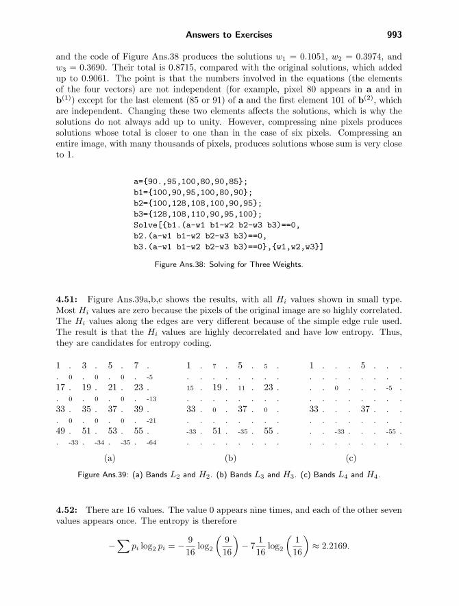
and the code of Figure Ans.38 produces the solutions w1 = 0.1051, w2 = 0.3974, andw3 = 0.3690. Their total is 0.8715, compared with the original solutions, which addedup to 0.9061. The point is that the numbers involved in the equations (the elementsof the four vectors) are not independent (for example, pixel 80 appears in a and inb(1)) except for the last element (85 or 91) of a and the first element 101 of b(2), whichare independent. Changing these two elements affects the solutions, which is why thesolutions do not always add up to unity. However, compressing nine pixels producessolutions whose total is closer to one than in the case of six pixels. Compressing anentire image, with many thousands of pixels, produces solutions whose sum is very closeto 1.
a={90.,95,100,80,90,85};b1={100,90,95,100,80,90};b2={100,128,108,100,90,95};b3={128,108,110,90,95,100};Solve[{b1.(a-w1 b1-w2 b2-w3 b3)==0,b2.(a-w1 b1-w2 b2-w3 b3)==0,b3.(a-w1 b1-w2 b2-w3 b3)==0},{w1,w2,w3}]
Figure Ans.38: Solving for Three Weights.
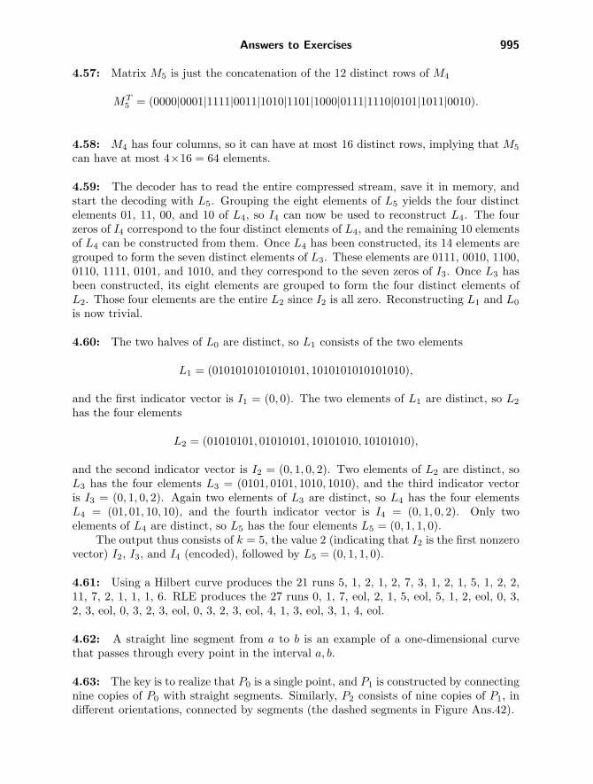
4.51: Figure Ans.39a,b,c shows the results, with all Hi values shown in small type.Most Hi values are zero because the pixels of the original image are so highly correlated.The Hi values along the edges are very different because of the simple edge rule used.The result is that the Hi values are highly decorrelated and have low entropy. Thus,they are candidates for entropy coding.
1 . 3 . 5 . 7 .. 0 . 0 . 0 . -5
17 . 19 . 21 . 23 .. 0 . 0 . 0 . -13
33 . 35 . 37 . 39 .. 0 . 0 . 0 . -21
49 . 51 . 53 . 55 .. -33 . -34 . -35 . -64
1 . 7 . 5 . 5 .. . . . . . . .15 . 19 . 11 . 23 .. . . . . . . .33 . 0 . 37 . 0 .. . . . . . . .-33 . 51 . -35 . 55 .. . . . . . . .
1 . . . 5 . . .. . . . . . . .. . 0 . . . -5 .. . . . . . . .33 . . . 37 . . .. . . . . . . .. . -33 . . . -55 .. . . . . . . .
(a) (b) (c)
Figure Ans.39: (a) Bands L2 and H2. (b) Bands L3 and H3. (c) Bands L4 and H4.
4.52: There are 16 values. The value 0 appears nine times, and each of the other sevenvalues appears once. The entropy is therefore
−∑
pi log2 pi = − 916
log2
(916
)− 7
116
log2
(116
)≈ 2.2169.

994 Answers to Exercises
Not very small, because seven of the 16 values have the same probability. In practice,values of an Hi difference band tend to be small, are both positive and negative, andare concentrated around zero, so their entropy is small.
4.53: Because the decoder needs to know how the encoder estimated X for each Hi
difference value. If the encoder uses one of three methods for prediction, it has to precedeeach difference value in the compressed stream with a code that tells the decoder whichmethod was used. Such a code can have variable size (for example, 0, 10, 11) buteven adding just one or two bits to each prediction reduces compression performancesignificantly, because each Hi value needs to be predicted, and the number of thesevalues is close to the size of the image.
4.54: The binary tree is shown in Figure Ans.40. From this tree, it is easy to see thatthe progressive image file is 3 6|5 7|7 7 10 5.
3,7
3 4 5 6 6 4 5 8
3,5 5,7
3,6
6,7 4,10 5,5
Figure Ans.40: A Binary Tree for an 8-Pixel Image.
4.55: They are shown in Figure Ans.41.
..
.
Figure Ans.41: The 15 6-Tuples With Two White Pixels.
4.56: No. An image with little or no correlation between the pixels will not compresswith quadrisection, even though the size of the last matrix is always small. Even withoutknowing the details of quadrisection we can confidently state that such an image willproduce a sequence of matrices Mj with few or no identical rows. In the extreme case,where the rows of any Mj are all distinct, each Mj will have four times the numberof rows of its predecessor. This will create indicator vectors Ij that get longer andlonger, thereby increasing the size of the compressed stream and reducing the overallcompression performance.
Answers to Exercises 995
4.57: Matrix M5 is just the concatenation of the 12 distinct rows of M4
MT5 = (0000|0001|1111|0011|1010|1101|1000|0111|1110|0101|1011|0010).
4.58: M4 has four columns, so it can have at most 16 distinct rows, implying that M5
can have at most 4×16 = 64 elements.
4.59: The decoder has to read the entire compressed stream, save it in memory, andstart the decoding with L5. Grouping the eight elements of L5 yields the four distinctelements 01, 11, 00, and 10 of L4, so I4 can now be used to reconstruct L4. The fourzeros of I4 correspond to the four distinct elements of L4, and the remaining 10 elementsof L4 can be constructed from them. Once L4 has been constructed, its 14 elements aregrouped to form the seven distinct elements of L3. These elements are 0111, 0010, 1100,0110, 1111, 0101, and 1010, and they correspond to the seven zeros of I3. Once L3 hasbeen constructed, its eight elements are grouped to form the four distinct elements ofL2. Those four elements are the entire L2 since I2 is all zero. Reconstructing L1 and L0
is now trivial.
4.60: The two halves of L0 are distinct, so L1 consists of the two elements
L1 = (0101010101010101, 1010101010101010),
and the first indicator vector is I1 = (0, 0). The two elements of L1 are distinct, so L2
has the four elements
L2 = (01010101, 01010101, 10101010, 10101010),
and the second indicator vector is I2 = (0, 1, 0, 2). Two elements of L2 are distinct, soL3 has the four elements L3 = (0101, 0101, 1010, 1010), and the third indicator vectoris I3 = (0, 1, 0, 2). Again two elements of L3 are distinct, so L4 has the four elementsL4 = (01, 01, 10, 10), and the fourth indicator vector is I4 = (0, 1, 0, 2). Only twoelements of L4 are distinct, so L5 has the four elements L5 = (0, 1, 1, 0).
The output thus consists of k = 5, the value 2 (indicating that I2 is the first nonzerovector) I2, I3, and I4 (encoded), followed by L5 = (0, 1, 1, 0).
4.61: Using a Hilbert curve produces the 21 runs 5, 1, 2, 1, 2, 7, 3, 1, 2, 1, 5, 1, 2, 2,11, 7, 2, 1, 1, 1, 6. RLE produces the 27 runs 0, 1, 7, eol, 2, 1, 5, eol, 5, 1, 2, eol, 0, 3,2, 3, eol, 0, 3, 2, 3, eol, 0, 3, 2, 3, eol, 4, 1, 3, eol, 3, 1, 4, eol.
4.62: A straight line segment from a to b is an example of a one-dimensional curvethat passes through every point in the interval a, b.
4.63: The key is to realize that P0 is a single point, and P1 is constructed by connectingnine copies of P0 with straight segments. Similarly, P2 consists of nine copies of P1, indifferent orientations, connected by segments (the dashed segments in Figure Ans.42).

996 Answers to Exercises
(a) (b) (c)
P0 P1
Figure Ans.42: The First Three Iterations of the Peano Curve.
4.64: Written in binary, the coordinates are (1101, 0110). We iterate four times, eachtime taking 1 bit from the x coordinate and 1 bit from the y coordinate to form an (x, y)pair. The pairs are 10, 11, 01, 10. The first one yields [from Table 4.170(1)] 01. Thesecond pair yields [also from Table 4.170(1)] 10. The third pair [from Table 4.170(1)]11, and the last pair [from Table 4.170(4)] 01. Thus, the result is 01|10|11|01 = 109.
4.65: Table Ans.43 shows that this traversal is based on the sequence 2114.
1: 2 ↑ 1 → 1 ↓ 42: 1 → 2 ↑ 2 ← 33: 4 ↓ 3 ← 3 ↑ 24: 3 ← 4 ↓ 4 → 1
Table Ans.43: The Four Orientations of H2.
4.66: This is straightforward
(00, 01, 11, 10) → (000, 001, 011, 010)(100, 101, 111, 110)→ (000, 001, 011, 010)(110, 111, 101, 100)→ (000, 001, 011, 010, 110, 111, 101, 100).
4.67: The gray area of Figure 4.171c is identified by the string 2011.
4.68: This particular numbering makes it easy to convert between the number of asubsquare and its image coordinates. (We assume that the origin is located at thebottom-left corner of the image and that image coordinates vary from 0 to 1.) As anexample, translating the digits of the number 1032 to binary results in (01)(00)(11)(10).The first bits of these groups constitute the x coordinate of the subsquare, and thesecond bits constitute the y coordinate. Thus, the image coordinates of subsquare1032 are x = .00112 = 3/16 and y = .10102 = 5/8, as can be directly verified fromFigure 4.171c.

Answers to Exercises 997
10050
500
1
1,2(0.25)0,1,2,3(1)0,1,2,3(0.5)
3(0.5)
2
Figure Ans.44: A Two-State Graph.
4.69: This is shown in Figure Ans.44.
4.70: This image is described by the function
f(x, y) ={
x + y, if x + y ≤ 1,0, if x + y > 1.
4.71: The graph has five states, so each transition matrix is of size 5×5. Directcomputation from the graph yields
W0 =
⎛⎜⎜⎜⎝
0 1 0 0 00 0.5 0 0 00 0 0 0 10 −0.5 0 0 1.50 −0.25 0 0 1
⎞⎟⎟⎟⎠ , W3 =
⎛⎜⎜⎜⎝
0 0 0 0 00 0 0 0 10 0 0 0 00 0 0 0 00 −1 0 0 1.5
⎞⎟⎟⎟⎠ ,
W1 = W2 =
⎛⎜⎜⎜⎝
0 0 1 0 00 0.25 0 0 0.50 0 0 1.5 00 0 −0.5 1.5 00 −0.375 0 0 1.25
⎞⎟⎟⎟⎠ .
The final distribution is the five-component vector
F = (0.25, 0.5, 0.375, 0.4125, 0.75)T .
4.72: One way to specify the center is to construct string 033 . . . 3. This yields
ψi(03 . . . 3) = (W0 ·W3 · · ·W3 ·F )i
=(
0.5 00 1
)(0.5 0.50 1
)· · ·(
0.5 0.50 1
)(0.51
)i
=(
0.5 00 1
)(0 10 1
)(0.51
)i
=(
0.51
)i
.

998 Answers to Exercises
dim=256;for i=1:dimfor j=1:dimm(i,j)=(i+j-2)/(2*dim-2);
endendm
Figure Ans.45: Matlab Code for a Matrix mi,j = (i + j)/2.
4.73: Figure Ans.45 shows Matlab code to compute a matrix such as those of Fig-ure 4.175.
4.74: A direct examination of the graph yields the ψi values
ψi(0) = (W0 ·F )i = (0.5, 0.25, 0.75, 0.875, 0.625)Ti ,
ψi(01) = (W0 ·W1 ·F )i = (0.5, 0.25, 0.75, 0.875, 0.625)Ti ,
ψi(1) = (W1 ·F )i = (0.375, 0.5, 0.61875, 0.43125, 0.75)Ti ,
ψi(00) = (W0 ·W0 ·F )i = (0.25, 0.125, 0.625, 0.8125, 0.5625)Ti ,
ψi(03) = (W0 ·W3 ·F )i = (0.75, 0.375, 0.625, 0.5625, 0.4375)Ti ,
ψi(3) = (W3 ·F )i = (0, 0.75, 0, 0, 0.625)Ti ,
and the f values
f(0) = I ·ψ(0) = 0.5, f(01) = I ·ψ(01) = 0.5, f(1) = I ·ψ(1) = 0.375,
f(00) = I ·ψ(00) = 0.25, f(03) = I ·ψ(03) = 0.75, f(3) = I ·ψ(3) = 0.
4.75: Figure Ans.46a,b shows the six states and all 21 edges. We use the notationi(q, t)j for the edge with quadrant number q and transformation t from state i to statej. This GFA is more complex than pervious ones since the original image is less self-similar.
4.76: The transformation can be written (x, y) → (x,−x + y), so (1, 0) → (1,−1),(3, 0) → (3,−3), (1, 1) → (1, 0) and (3, 1) → (3,−2). Thus, the original rectangle istransformed into a parallelogram.
4.77: The explanation is that the two sets of transformations produce the sameSierpinski triangle but at different sizes and orientations.
4.78: All three transformations shrink an image to half its original size. In addition,w2 and w3 place two copies of the shrunken image at relative displacements of (0, 1/2)and (1/2, 0), as shown in Figure Ans.47. The result is the familiar Sierpinski gasket butin a different orientation.

Answers to Exercises 999
4
0 1
35
2
0
1
2
3
0
1
2
3
0
1
2
3
0
1
2
3
0
1
2
3
0
1
2
3(1,0) (2,2)
(2,1)(3,1)
(0,0) (3,0)
(0,0) (3,0)
(0,1) (3,3)
(1,0) (2,2)
(0,1) (3,3)
(1,6)
(0,7)
(0,0) (0,6)
(2,0) (2,6)
(0,0) (0,6)
(2,0) (2,6)
(0,0)
(0,0)
(3,0)
(0,0)(0,8)
(0,0)(2,0)
(2,1)(3,1)
(0,0)(2,0)
(2,4)
(1,6)
(0,7)
(3,0)
(2,4)
(0,0)(0,8)
(a)
Start state
0 12
4 5 3
(b)
0(0,0)1 0(3,0)1 0(0,1)2 0(1,0)2 0(2,2)2 0(3,3)2 1(0,7)31(1,6)3 1(2,4)3 1(3,0)3 2(0,0)4 2(2,0)4 2(2,1)4 2(3,1)43(0,0)5 4(0,0)5 4(0,6)5 4(2,0)5 4(2,6)5 5(0,0)5 5(0,8)5
Figure Ans.46: A GFA for Exercise 4.75.
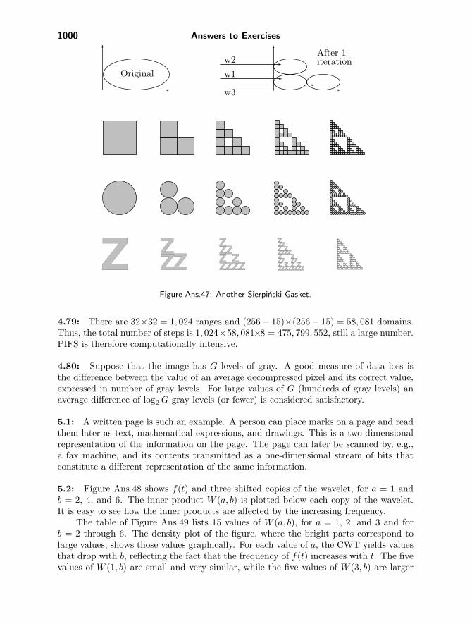
1000 Answers to Exercises
Originalw2
w1
w3
After 1iteration
Z ZZZ Z
ZZZZZZZZ Z
ZZZZZZZZ
ZZZZZZZZZ
ZZZZZZZZZ Z
ZZZZZZZZ
ZZZZZZZZZ
ZZZZZZZZZ
ZZZZZZZZZ
ZZZZZZZZZ
ZZZZZZZZZ
ZZZZZZZZZ
ZZZZZZZZZ
ZZZZZZZZZ
Figure Ans.47: Another Sierpinski Gasket.
4.79: There are 32×32 = 1, 024 ranges and (256− 15)×(256− 15) = 58, 081 domains.Thus, the total number of steps is 1, 024×58, 081×8 = 475, 799, 552, still a large number.PIFS is therefore computationally intensive.
4.80: Suppose that the image has G levels of gray. A good measure of data loss isthe difference between the value of an average decompressed pixel and its correct value,expressed in number of gray levels. For large values of G (hundreds of gray levels) anaverage difference of log2 G gray levels (or fewer) is considered satisfactory.
5.1: A written page is such an example. A person can place marks on a page and readthem later as text, mathematical expressions, and drawings. This is a two-dimensionalrepresentation of the information on the page. The page can later be scanned by, e.g.,a fax machine, and its contents transmitted as a one-dimensional stream of bits thatconstitute a different representation of the same information.
5.2: Figure Ans.48 shows f(t) and three shifted copies of the wavelet, for a = 1 andb = 2, 4, and 6. The inner product W (a, b) is plotted below each copy of the wavelet.It is easy to see how the inner products are affected by the increasing frequency.
The table of Figure Ans.49 lists 15 values of W (a, b), for a = 1, 2, and 3 and forb = 2 through 6. The density plot of the figure, where the bright parts correspond tolarge values, shows those values graphically. For each value of a, the CWT yields valuesthat drop with b, reflecting the fact that the frequency of f(t) increases with t. The fivevalues of W (1, b) are small and very similar, while the five values of W (3, b) are larger

Answers to Exercises 1001
2 4 6 8 10
Figure Ans.48: An Inner Product for a = 1 and b = 2, 4, 6.
a b = 2 3 4 5 61 0.032512 0.000299 1.10923×10⁻⁶ 2.73032×10⁻⁹ 8.33866×10⁻¹¹
2 0.510418 0.212575 0.0481292 0.00626348 0.000480973 0.743313 0.629473 0.380634 0.173591 0.064264
3 4
2
1
5 6b=2
a=3
Figure Ans.49: Fifteen Values and a Density Plot of W (a, b).

1002 Answers to Exercises
and differ more. This shows how scaling the wavelet up makes the CWT more sensitiveto frequency changes in f(t).
5.3: Figure 5.11c shows these wavelets.
5.4: Figure Ans.50a shows a simple, 8×8 image with one diagonal line above the maindiagonal. Figure Ans.50b,c shows the first two steps in its pyramid decomposition. Itis obvious that the transform coefficients in the bottom-right subband (HH) indicate adiagonal artifact located above the main diagonal. It is also easy to see that subbandLL is a low-resolution version of the original image.
12 16 12 12 12 12 12 1212 12 16 12 12 12 12 1212 12 12 16 12 12 12 1212 12 12 12 16 12 12 1212 12 12 12 12 16 12 1212 12 12 12 12 12 16 1212 12 12 12 12 12 12 1612 12 12 12 12 12 12 12
14 12 12 12 4 0 0 012 14 12 12 0 4 0 012 14 12 12 0 4 0 012 12 14 12 0 0 4 012 12 14 12 0 0 4 012 12 12 14 0 0 0 412 12 12 14 0 0 0 412 12 12 12 0 0 0 0
13 13 12 12 2 2 0 012 13 13 12 0 2 2 012 12 13 13 0 0 2 212 12 12 13 0 0 0 22 2 0 0 4 4 0 00 2 2 0 0 4 4 00 0 2 2 0 0 4 40 0 0 2 0 0 0 4
(a) (b) (c)
Figure Ans.50: The Subband Decomposition of a Diagonal Line.
5.5: The average can easily be calculated. It turns out to be 131.375, which is exactly1/8 of 1051. The reason the top-left transform coefficient is eight times the averageis that the Matlab code that did the calculations uses
√2 instead of 2 (see function
individ(n) in Figure 5.22).
5.6: Figure Ans.51a–c shows the results of reconstruction from 3277, 1639, and 820coefficients, respectively. Despite the heavy loss of wavelet coefficients, only a very smallloss of image quality is noticeable. The number of wavelet coefficients is, of course, thesame as the image resolution 128×128 = 16, 384. Using 820 out of 16,384 coefficientscorresponds to discarding 95% of the smallest of the transform coefficients (notice, how-ever, that some of the coefficients were originally zero, so the actual loss may amountto less than 95%).
5.7: The Matlab code of Figure Ans.52 calculates W as the product of the threematrices A1, A2, and A3 and computes the 8×8 matrix of transform coefficients. Noticethat the top-left value 131.375 is the average of all the 64 image pixels.
5.8: The vector x = (. . . , 1,−1, 1,−1, 1, . . .) of alternating values is transformed by thelowpass filter H0 to a vector of all zeros.

Answers to Exercises 1003
0 20 40 60 80 100 120
0
20
40
60
80
100
120
nz = 3277
0 20 40 60 80 100 120
0
20
40
60
80
100
120
nz = 1639
0 20 40 60 80 100 120
0
20
40
60
80
100
120
nz = 820
(a)
(b)
(c)
0
20
40
60
80
100
120
0
20
40
60
80
100
120
0
20
40
60
80
100
120
0 20 40 60 80 100 120
0 20 40 60 80 100 120
0 20 40 60 80 100 120
nz=3277
nz=1639
nz=820
Figure Ans.51: Three Lossy Reconstructions of the 128×128 Lena Image.

1004 Answers to Exercises
cleara1=[1/2 1/2 0 0 0 0 0 0; 0 0 1/2 1/2 0 0 0 0;0 0 0 0 1/2 1/2 0 0; 0 0 0 0 0 0 1/2 1/2;1/2 -1/2 0 0 0 0 0 0; 0 0 1/2 -1/2 0 0 0 0;0 0 0 0 1/2 -1/2 0 0; 0 0 0 0 0 0 1/2 -1/2];% a1*[255; 224; 192; 159; 127; 95; 63; 32];a2=[1/2 1/2 0 0 0 0 0 0; 0 0 1/2 1/2 0 0 0 0;1/2 -1/2 0 0 0 0 0 0; 0 0 1/2 -1/2 0 0 0 0;0 0 0 0 1 0 0 0; 0 0 0 0 0 1 0 0;0 0 0 0 0 0 1 0; 0 0 0 0 0 0 0 1];a3=[1/2 1/2 0 0 0 0 0 0; 1/2 -1/2 0 0 0 0 0 0;0 0 1 0 0 0 0 0; 0 0 0 1 0 0 0 0;0 0 0 0 1 0 0 0; 0 0 0 0 0 1 0 0;0 0 0 0 0 0 1 0; 0 0 0 0 0 0 0 1];w=a3*a2*a1;dim=8; fid=fopen(’8x8’,’r’);img=fread(fid,[dim,dim])’; fclose(fid);w*img*w’ % Result of the transform
131.375 4.250 −7.875 −0.125 −0.25 −15.5 0 −0.250 0 0 0 0 0 0 00 0 0 0 0 0 0 00 0 0 0 0 0 0 0
12.000 59.875 39.875 31.875 15.75 32.0 16 15.7512.000 59.875 39.875 31.875 15.75 32.0 16 15.7512.000 59.875 39.875 31.875 15.75 32.0 16 15.7512.000 59.875 39.875 31.875 15.75 32.0 16 15.75
Figure Ans.52: Code and Results for the Calculation of Matrix W and Transform W ·I ·WT .
5.9: For these filters, rules 1 and 2 imply
h20(0) + h2
0(1) + h20(2) + h2
0(3) + h20(4) + h2
0(5) + h20(6) + h2
0(7) = 1,h0(0)h0(2) + h0(1)h0(3) + h0(2)h0(4) + h0(3)h0(5) + h0(4)h0(6) + h0(5)h0(7) = 0,
h0(0)h0(4) + h0(1)h0(5) + h0(2)h0(6) + h0(3)h0(7) = 0,h0(0)h0(6) + h0(1)h0(7) = 0,
and rules 3–5 yield
f0 =(h0(7), h0(6), h0(5), h0(4), h0(3), h0(2), h0(1), h0(0)
),
h1 =(−h0(7), h0(6),−h0(5), h0(4),−h0(3), h0(2),−h0(1), h0(0)
),
f1 =(h0(0),−h0(1), h0(2),−h0(3), h0(4),−h0(5), h0(6),−h0(7)
).
The eight coefficients are listed in Table 5.35 (this is the Daubechies D8 filter).
5.10: Figure Ans.53 lists the Matlab code of the inverse wavelet transform functioniwt1(wc,coarse,filter) and a test.

Answers to Exercises 1005
function dat=iwt1(wc,coarse,filter)% Inverse Discrete Wavelet Transformdat=wc(1:2^coarse);n=length(wc); j=log2(n);for i=coarse:j-1dat=ILoPass(dat,filter)+ ...IHiPass(wc((2^(i)+1):(2^(i+1))),filter);
end
function f=ILoPass(dt,filter)f=iconv(filter,AltrntZro(dt));
function f=IHiPass(dt,filter)f=aconv(mirror(filter),rshift(AltrntZro(dt)));
function sgn=mirror(filt)% return filter coefficients with alternating signssgn=-((-1).^(1:length(filt))).*filt;
function f=AltrntZro(dt)% returns a vector of length 2*n with zeros% placed between consecutive valuesn =length(dt)*2; f =zeros(1,n);f(1:2:(n-1))=dt;
Figure Ans.53: Code for the 1D Inverse Discrete Wavelet Transform.
A simple test of iwt1 isn=16; t=(1:n)./n;dat=sin(2*pi*t)filt=[0.4830 0.8365 0.2241 -0.1294];wc=fwt1(dat,1,filt)rec=iwt1(wc,1,filt)
5.11: Figure Ans.54 shows the result of blurring the “lena” image. Parts (a) and (b)show the logarithmic multiresolution tree and the subband structure, respectively. Part(c) shows the results of the quantization. The transform coefficients of subbands 5–7have been divided by two, and all the coefficients of subbands 8–13 have been cleared. Wecan say that the blurred image of part (d) has been reconstructed from the coefficientsof subbands 1–4 (1/64th of the total number of transform coefficients) and half of thecoefficients of subbands 5–7 (half of 3/64, or 3/128). On average, the image has beenreconstructed from 5/128 ≈ 0.039 or 3.9% of the transform coefficients. Notice that theDaubechies D8 filter was used in the calculations. Readers are encouraged to use thiscode and experiment with the performance of other filters.
5.12: They are written in the form a-=b/2; b+=a;.

1006 Answers to Exercises
(c) (d)
1 23 4
(a) (b)
6 75
8
1011
1312
9
H0
H1
↓2
↓2
H0
H1
↓2
↓2
H0
H1
↓2
↓2
H0
H1
↓2
↓2
Figure Ans.54: Blurring as a Result of Coarse Quantization.
clear, colormap(gray);filename=’lena128’; dim=128;fid=fopen(filename,’r’);img=fread(fid,[dim,dim])’;filt=[0.23037,0.71484,0.63088,-0.02798, ...-0.18703,0.03084,0.03288,-0.01059];
fwim=fwt2(img,3,filt);figure(1), imagesc(fwim), axis squarefwim(1:16,17:32)=fwim(1:16,17:32)/2;fwim(1:16,33:128)=0;fwim(17:32,1:32)=fwim(17:32,1:32)/2;fwim(17:32,33:128)=0;fwim(33:128,:)=0;
figure(2), colormap(gray), imagesc(fwim)rec=iwt2(fwim,3,filt);figure(3), colormap(gray), imagesc(rec)
Code for Figure Ans.54.

Answers to Exercises 1007
5.13: We sum Equation (5.13) over all the values of l to get
2j−1−1∑l=0
sj−1,l =2j−1−1∑
l=0
(sj,2l + dj−1,l/2) =12
2j−1−1∑l=0
(sj,2l + sj,2l+1) =12
2j−1∑l=0
sj,l. (Ans.1)
Therefore, the average of set sj−1 equals
12j−1
2j−1−1∑l=0
sj−1,l =1
2j−1
12
2j−1∑l=0
sj,l =12j
2j−1∑l=0
sj,l
the average of set sj .
5.14: The code of Figure Ans.55 produces the expression
0.0117P1 − 0.0977P2 + 0.5859P3 + 0.5859P4 − 0.0977P5 + 0.0117P6.
Clear[p,a,b,c,d,e,f];p[t_]:=a t^5+b t^4+c t^3+d t^2+e t+f;Solve[{p[0]==p1, p[1/5.]==p2, p[2/5.]==p3,p[3/5.]==p4, p[4/5.]==p5, p[1]==p6}, {a,b,c,d,e,f}];sol=ExpandAll[Simplify[%]];Simplify[p[0.5] /.sol]
Figure Ans.55: Code for a Degree-5 Interpolating Polynomial.
5.15: The Matlab code of Figure Ans.56 does that and produces the transformedinteger vector y = (111,−1, 84, 0, 120, 25, 84, 3). The inverse transform generates vectorz that is identical to the original data x. Notice how the detail coefficients are muchsmaller than the weighted averages. Notice also that Matlab arrays are indexed from1, whereas the discussion in the text assumes arrays indexed from 0. This causes thedifference in index values in Figure Ans.56.
5.16: For the case MC = 3, the first six images g0 through g5 will have dimensions
(3 · 25 + 1× 4 · 25 + 1) = 97× 129, 49× 65, 25× 33, 13× 17, and 7× 9.
5.17: In the sorting pass of the third iteration the encoder transmits the number l = 3(the number of coefficients ci,j in our example that satisfy 212 ≤ |ci,j | < 213), followedby the three pairs of coordinates (3, 3), (4, 2), and (4, 1) and by the signs of the threecoefficients. In the refinement step it transmits the six bits cdefgh. These are the 13thmost significant bits of the coefficients transmitted in all the previous iterations.

1008 Answers to Exercises
clear;N=8; k=N/2;x=[112,97,85,99,114,120,77,80];% Forward IWT into yfor i=0:k-2,y(2*i+2)=x(2*i+2)-floor((x(2*i+1)+x(2*i+3))/2);end;y(N)=x(N)-x(N-1);y(1)=x(1)+floor(y(2)/2);for i=1:k-1,y(2*i+1)=x(2*i+1)+floor((y(2*i)+y(2*i+2))/4);end;% Inverse IWT into zz(1)=y(1)-floor(y(2)/2);for i=1:k-1,z(2*i+1)=y(2*i+1)-floor((y(2*i)+y(2*i+2))/4);end;for i=0:k-2,z(2*i+2)=y(2*i+2)+floor((z(2*i+1)+x(2*i+3))/2);end;z(N)=y(N)+z(N-1);
Figure Ans.56: Matlab Code for Forward and Inverse IWT.
The information received so far enables the decoder to further improve the 16 ap-proximate coefficients. The first nine become
c2,3 = s1ac0 . . . 0, c3,4 = s1bd0 . . . 0, c3,2 = s01e00 . . . 0,
c4,4 = s01f00 . . . 0, c1,2 = s01g00 . . . 0, c3,1 = s01h00 . . . 0,
c3,3 = s0010 . . . 0, c4,2 = s0010 . . . 0, c4,1 = s0010 . . . 0,
and the remaining seven are not changed.
5.18: The simple equation 10×220×8 = (500x)×(500x)×8 is solved to yield x2 = 40square inches. If the card is square, it is approximately 6.32 inches on a side. Sucha card has 10 rolled impressions (about 1.5 × 1.5 each), two plain impressions of thethumbs (about 0.875×1.875 each), and simultaneous impressions of both hands (about3.125×1.875 each). All the dimensions are in inches.
5.19: The bit of 10 is encoded, as usual, in pass 2. The bit of 1 is encoded in pass 1since this coefficient is still insignificant but has significant neighbors. This bit is 1, socoefficient 1 becomes significant (a fact that is not used later). Also, this bit is the first1 of this coefficient, so the sign bit of the coefficient is encoded following this bit. Thebits of coefficients 3 and −7 are encoded in pass 2 since these coefficients are significant.
6.1: It is easy to calculate that 525× 4/3 = 700 pixels.

Answers to Exercises 1009
6.2: The vertical height of the picture on the author’s 27 in. television set is 16 in.,which translates to a viewing distance of 7.12× 16 = 114 in. or about 9.5 feet. It is easyto see that individual scan lines are visible at any distance shorter than about 6 feet.
6.3: Three common examples are: (1) Surveillance camera, (2) an old, silent moviebeing restored and converted from film to video, and (3) a video presentation takenunderwater.
6.4: The golden ratio φ ≈ 1.618 has traditionally been considered the aspect ratio thatis most pleasing to the eye. This suggests that 1.77 is the better aspect ratio.
6.5: Imagine a camera panning from left to right. New objects will enter the field ofview from the right all the time. A block on the right side of the frame may thereforecontain objects that did not exist in the previous frame.
6.6: Since (4, 4) is at the center of the “+”, the value of s is halved, to 2. The next stepsearches the four blocks labeled 4, centered on (4, 4). Assuming that the best match isat (6, 4), the two blocks labeled 5 are searched. Assuming that (6, 4) is the best match,s is halved to 1, and the eight blocks labeled 6 are searched. The diagram shows thatthe best match is finally found at location (7, 4).
6.7: This figure consists of 18×18 macroblocks, and each macroblock constitutes six8×8 blocks of samples. The total number of samples is therefore 18×18×6×64 = 124, 416.
6.8: The size category of zero is 0, so code 100 is emitted, followed by zero bits. Thesize category of 4 is 3, so code 110 is first emitted, followed by the three least-significantbits of 4, which are 100.
6.9: The zigzag sequence is
118, 2, 0,−2, 0, . . . , 0︸ ︷︷ ︸13
,−1, 0, . . . .
The run-level pairs are (0, 2), (1,−2), and (13,−1), so the final codes are (notice thesign bits following the run-level codes)
0100 0|000110 1|00100000 1|10,
(without the vertical bars).
6.10: There are no nonzero coefficients, no run-level codes, just the 2-bit EOB code.However, in nonintra coding, such a block is encoded in a special way.
7.1: An average book may have 60 characters per line, 45 lines per page, and 400 pages.This comes to 60× 45× 400 = 1, 080, 000 characters, requiring one byte of storage each.

1010 Answers to Exercises
7.2: The period of a wave is its speed divided by its frequency. For sound we get
34380 cm/s22000 Hz
= 1.562 cm,34380
20= 1719 cm.
7.3: The (base-10) logarithm of x is a number y such that 10y = x. The number 2 isthe logarithm of 100 since 102 = 100. Similarly, 0.3 is the logarithm of 2 since 100.3 = 2.Also, The base-b logarithm of x is a number y such that by = x (for any real b > 1).
7.4: Each doubling of the sound intensity increases the dB level by 3. Therefore, thedifference of 9 dB (3 + 3 + 3) between A and B corresponds to three doublings of thesound intensity. Thus, source B is 2·2·2 = 8 times louder than source A.
7.5: Each 0 would result in silence and each sample of 1, in the same tone. The resultwould be a nonuniform buzz. Such sounds were common on early personal computers.
7.6: Such an experiment should be repeated with several persons, preferably of differentages. The person should be placed in a sound insulated chamber, and a pure tone offrequency f should be played. The amplitude of the tone should be gradually increasedfrom zero until the person can just barely hear it. If this happens at a decibel valued, point (d, f) should be plotted. This should be repeated for many frequencies until agraph similar to Figure 7.5a is obtained.
7.7: We first select identical items. If all s(t − i) equal s, Equation (7.7) yields thesame s. Next, we select values on a straight line. Given the four values a, a + 2, a + 4,and a + 6, Equation (7.7) yields a + 8, the next linear value. Finally, we select valuesroughly equally-spaced on a circle. The y coordinates of points on the first quadrant of acircle can be computed by y =
√r2 − x2. We select the four points with x coordinates 0,
0.08r, 0.16r, and 0.24r, compute their y coordinates for r = 10, and substitute them inEquation (7.7). The result is 9.96926, compared to the actual y coordinate for x = 0.32rwhich is
√r2 − (0.32r)2 = 9.47418, a difference of about 5%. The code that did the
computations is shown in Figure Ans.57.
(* Points on a circle. Used in exercise to check4th-order prediction in FLAC *)
r = 10;ci[x_] := Sqrt[100 - x^2];ci[0.32r]4ci[0] - 6ci[0.08r] + 4ci[0.16r] - ci[0.24r]
Figure Ans.57: Code for Checking 4th-Order Prediction.

Answers to Exercises 1011
7.8: Imagine that the sound being compressed contains one second of a pure tone(just one frequency). This second will be digitized to 44,100 consecutive samples perchannel. The samples indicate amplitudes, so they don’t have to be the same. However,after filtering, only one subband (although in practice perhaps two subbands) will havenonzero signals. All the other subbands correspond to different frequencies, so they willhave signals that are either zero or very close to zero.
7.9: Assuming that a noise level P1 translates to x decibels
20 log(
P1
P2
)= x dB SPL,
results in the relation
20 log
(3√
2P1
P2
)= 20
[log10
3√
2 + log(
P1
P2
)]= 20(0.1 + x/20) = x + 2.
Thus, increasing the sound level by a factor of 3√
2 increases the decibel level by 2 dB SPL.
7.10: For a sampling rate of 44,100 samples/sec, the calculations are similar. Thedecoder has to decode 44,100/384 ≈ 114.84 frames per second. Thus, each frame has tobe decoded in approximately 8.7 ms. In order to output 114.84 frames in 64,000 bits,each frame must have Bf = 557 bits available to encode it. Thus, the number of slotsper frame is 557/32 ≈ 17.41. Thus, the last (18th) slot is not full and has to padded.
7.11: Table 7.58 shows that the scale factor is 111 and the select information is 2. Thethird rule in Table 7.59 shows that a scfsi of 2 means that only one scale factor wascoded, occupying just six bits in the compressed output. The decoder assigns these sixbits as the values of all three scale factors.
7.12: Typical layer II parameters are (1) a sampling rate of 48,000 samples/sec, (2) abitrate of 64,000 bits/sec, and (3) 1,152 quantized signals per frame. The decoder has todecode 48,000/1152 = 41.66 frames per second. Thus, each frame has to be decoded in24 ms. In order to output 41.66 frames in 64,000 bits, each frame must have Bf = 1,536bits available to encode it.
7.13: A program to play .mp3 files is an MPEG layer III decoder, not an encoder.Decoding is much simpler since it does not use a psychoacoustic model, nor does it haveto anticipate preechoes and maintain the bit reservoir.
8.1: Because the original string S can be reconstructed from L but not from F.
8.2: A direct application of Equation (8.1) eight more times produces:
S[10-1-2]=L[T2[I]]=L[T[T1[I]]]=L[T[7]]=L[6]=i;S[10-1-3]=L[T3[I]]=L[T[T2[I]]]=L[T[6]]=L[2]=m;S[10-1-4]=L[T4[I]]=L[T[T3[I]]]=L[T[2]]=L[3]=�;

1012 Answers to Exercises
S[10-1-5]=L[T5[I]]=L[T[T4[I]]]=L[T[3]]=L[0]=s;S[10-1-6]=L[T6[I]]=L[T[T5[I]]]=L[T[0]]=L[4]=s;S[10-1-7]=L[T7[I]]=L[T[T6[I]]]=L[T[4]]=L[5]=i;S[10-1-8]=L[T8[I]]=L[T[T7[I]]]=L[T[5]]=L[1]=w;S[10-1-9]=L[T9[I]]=L[T[T8[I]]]=L[T[1]]=L[9]=s;
The original string swiss�miss is indeed reproduced in S from right to left.
8.3: Figure Ans.58 shows the rotations of S and the sorted matrix. The last column, Lof Ans.58b happens to be identical to S, so S=L=sssssssssh. Since A=(s,h), a move-to-front compression of L yields C = (1, 0, 0, 0, 0, 0, 0, 0, 0, 1). Since C contains just thetwo values 0 and 1, they can serve as their own Huffman codes, so the final result is1000000001, 1 bit per character!
ssssssssshsssssssshsssssssshsssssssshsssssssshsssssssshsssssssshsssssssshsssssssshsssssssshsssssssss
hsssssssssshsssssssssshsssssssssshsssssssssshsssssssssshsssssssssshsssssssssshsssssssssshssssssssssh
(a) (b)Figure Ans.58: Permutations of “sssssssssh”.
8.4: The encoder starts at T[0], which contains 5. The first element of L is thus the lastsymbol of permutation 5. This permutation starts at position 5 of S, so its last elementis in position 4. The encoder thus has to go through symbols S[T[i-1]] for i = 0, . . . , n−1,where the notation i − 1 should be interpreted cyclically (i.e., 0 − 1 should be n − 1).As each symbol S[T[i-1]] is found, it is compressed using move-to-front. The value of Iis the position where T contains 0. In our example, T[8]=0, so I=8.
8.5: The first element of a triplet is the distance between two dictionary entries, theone best matching the content and the one best matching the context. In this case thereis no content match, no distance, so any number could serve as the first element, 0 beingthe best (smallest) choice.
8.6: because the three lines are sorted in ascending order. The bottom two lines ofTable 8.13c are not in sorted order. This is why the zz...z part of string S must bepreceded and followed by complementary bits.
8.7: The encoder places S between two entries of the sorted associative list and writesthe (encoded) index of the entry above or below S on the compressed stream. The fewerthe number of entries, the smaller this index, and the better the compression.

Answers to Exercises 1013
8.8: Context 5 is compared to the three remaining contexts 6, 7, and 8, and it is mostsimilar to context 6 (they share a suffix of “b”). Context 6 is compared to 7 and 8 and,since they don’t share any suffix, context 7, the shorter of the two, is selected. Theremaining context 8 is, of course, the last one in the ranking. The final context rankingis
1 → 3 → 4 → 0 → 5 → 6 → 7 → 8.
8.9: Equation (8.3) shows that the third “a” is assigned rank 1 and the “b” and “a”following it are assigned ranks 2 and 3, respectively.
8.10: Table Ans.59 shows the sorted contexts. Equation (Ans.2) shows the contextranking at each step.
0u
, 0u
→ 2b
, 1l
→ 3b
→ 0u
,
0u
→ 2l
→ 3a
→ 4b
, 2l
→ 4a
→ 1d
→ 5b
→ 0u
,(Ans.2)
3i
→ 5a
→ 2l
→ 6b
→ 5d
→ 0u
.
The final output is “u 2 b 3 l 4 a 5 d 6 i 6.” Notice that each of the distinct input symbolsappears once in this output in raw format.
0 λ u1 u x
(a)
0 λ u1 ub x2 u b
(b)
0 λ u1 ub l2 ubl x3 u b
(c)
0 λ u1 ubla x2 ub l3 ubl a4 u b
(d)
0 λ u1 ubla d2 ub l3 ublad x4 ubl a5 u b
(e)
0 λ u1 ubla d2 ub l3 ublad i4 ubladi x5 ubl a6 u b
(f)
Table Ans.59: Constructing the Sorted Lists for ubladiu.
8.11: All n1 bits of string L1 need be written on the output stream. This alreadyshows that there is going to be no compression. String L2 consists of n1/k 1’s, so all ofit has to be written on the output stream. String L3 similarly consists of n1/k2 1’s, andso on. Thus, the size of the output stream is
n1 +n1
k+
n1
k2+
n1
k3+ · · ·+ n1
km= n1
km+1 − 1km(k − 1)
,

1014 Answers to Exercises
for some value of m. The limit of this expression, when m → ∞, is n1k/(k − 1). Fork = 2 this equals 2n1. For larger values of k this limit is always between n1 and 2n1.
For the curious reader, here is how the sum above is computed. Given the series
S =m∑
i=0
1ki
= 1 +1k
+1k2
+1k3
+ · · ·+ 1km−1
+1
km,
we multiply both sides by 1/k
S
k=
1k
+1k2
+1k3
+ · · ·+ 1km
+1
km+1= S +
1km+1
− 1,
and subtractS
k(k − 1) =
km+1 − 1km+1
→ S =km+1 − 1km(k − 1)
.
8.12: The input stream consists of:1. A run of three zero groups, coded as 10|1 since 3 is in second position in class 2.2. The nonzero group 0100, coded as 111100.3. Another run of three zero groups, again coded as 10|1.4. The nonzero group 1000, coded as 01100.5. A run of four zero groups, coded as 010|00 since 4 is in first position in class 3.6. 0010, coded as 111110.7. A run of two zero groups, coded as 10|0.
The output is thus the 31-bit string 1011111001010110001000111110100.
8.13: The input stream consists of:1. A run of three zero groups, coded as R2R1 or 101|11.2. The nonzero group 0100, coded as 00100.3. Another run of three zero groups, again coded as 101|11.4. The nonzero group 1000, coded as 01000.5. A run of four zero groups, coded as R4 = 1001.6. 0010, coded as 00010.7. A run of two zero groups, coded as R2 = 101.
The output is thus the 32-bit string 10111001001011101000100100010101.
8.14: The input stream consists of:1. A run of three zero groups, coded as F3 or 1001.2. The nonzero group 0100, coded as 00100.3. Another run of three zero groups, again coded as 1001.4. The nonzero group 1000, coded as 01000.5. A run of four zero groups, coded as F3F1 = 1001|11.6. 0010, coded as 00010.7. A run of two zero groups, coded as F2 = 101.
The output is thus the 32-bit string 10010010010010100010011100010101.

Answers to Exercises 1015
8.15: Yes, if they are located in different quadrants or subquadrants. Pixels 123 and301, for example, are adjacent in Figure 4.157 but have different prefixes.
8.16: No, because all prefixes have the same probability of occurrence. In our examplethe prefixes are four bits long and all 16 possible prefixes have the same probabilitybecause a pixel may be located anywhere in the image. A Huffman code constructedfor 16 equally-probable symbols has an average size of four bits per symbol, so nothingwould be gained. The same is true for suffixes.
8.17: This is possible, but it places severe limitations on the size of the string. In orderto rearrange a one-dimensional string into a four-dimensional cube, the string size shouldbe 24n. If the string size happens to be 24n + 1, it has to be extended to 24(n+1), whichincreases its size by a factor of 16. It is possible to rearrange the string into a rectangularbox, not just a cube, but then its size will have to be of the form 2n12n22n32n4 wherethe four ni’s are integers.
8.18: The LZW algorithm, which starts with the entire alphabet stored at the begin-ning of its dictionary, is an example of such a method. However, an adaptive version ofLZW can be designed to compress words instead of individual characters.
8.19: A better choice for the coordinates may be relative values (or offsets). Each (x, y)pair may specify the position of a character relative to its predecessor. This results insmaller numbers for the coordinates, and smaller numbers are easier to compress.
8.20: There may be such letters in other, “exotic” alphabets, but a more commonexample is a rectangular box enclosing text. The four rules that constitute such a boxshould be considered a mark, but the text characters inside the box should be identifiedas separate marks.
8.21: This guarantees that the two probabilities will add up to 1.
8.22: Figure Ans.60 shows how state A feeds into the new state D′ which, in turn,feeds into states E and F . Notice how states B and C haven’t changed. Since the newstate D′ is identical to D, it is possible to feed A into either D or D′ (cloning can bedone in two different but identical ways). The original counts of state D should now bedivided between D and D′ in proportion to the counts of the transitions A → D andB,C → D.
8.23: Figure Ans.61 shows the new state 6 after the operation 1, 1 → 6. Its 1-outputis identical to that of state 1, and its 0-output is a copy of the 0-output of state 3.
8.24: A precise answer requires many experiments with various data files. A littlethinking, though, shows that the larger k, the better the initial model that is createdwhen the old one is discarded. Larger values of k thus minimize the loss of compression.However, very large values may produce an initial model that is already large and cannotgrow much. The best value for k is therefore one that produces an initial model largeenough to provide information about recent correlations in the data, but small enoughso it has room to grow before it too has to be discarded.

1016 Answers to Exercises
0
1
0B
AE
C
D F
D’
1
1
0
1
0B
AE
C
FD’
D0
0
0
0
Figure Ans.60: New State D’ Cloned.
0
1652 0
13
01
00 1
1
1
0
40
10
1
Figure Ans.61: State 6 Added.
8.25: The number of marked points can be written 8(1+2+3+5+8+13) = 256 andthe numbers in parentheses are the Fibonacci numbers.
8.26: The conditional probability P (Di|Di) is very small. A segment pointing indirection Di can be preceded by another segment pointing in the same direction only ifthe original curve is straight or very close to straight for more than 26 coordinate units(half the width of grid S13).
8.27: We observe that a point has two coordinates. If each coordinate occupies eightbits, then the use of Fibonacci numbers reduces the 16-bit coordinates to an 8-bit num-ber, a compression ratio of 0.5. The use of Huffman codes can typically reduce this 8-bitnumber to (on average) a 4-bit code, and the use of the Markov model can perhaps cutthis by another bit. The result is an estimated compression ratio of 3/16 = 0.1875. Ifeach coordinate is a 16-bit number, then this ratio improves to 3/32 = 0.09375.
8.28: The resulting, shorter grammar is shown in Figure Ans.62. It is one rule andone symbol shorter.
Input Grammar
S→ abcdbcabcdbc S→ CCA→ bcC→ aAdA
Figure Ans.62: Improving the Grammar of Figure 8.41.

Answers to Exercises 1017
8.29: Because generating rule C has made rule B underused (i.e., used just once).
8.30: Rule S consists of two copies of rule A. The first time rule A is encountered, itscontents aBdB are sent. This involves sending rule B twice. The first time rule B is sent,its contents bc are sent (and the decoder does not know that the string bc it is receivingis the contents of a rule). The second time rule B is sent, the pair (1, 2) is sent (offset 1,count 2). The decoder identifies the pair and uses it to set up the rule 1→ bc. Sendingthe first copy of rule A therefore amounts to sending abcd(1, 2). The second copy of ruleA is sent as the pair (0, 4) since A starts at offset 0 in S and its length is 4. The decoderidentifies this pair and uses it to set up the rule 2→ a1d1 . The final result is thereforeabcd(1, 2)(0, 4).
8.31: In each of these cases, the encoder removes one edge from the boundary andinserts two new edges. There is a net gain of one edge.
8.32: They create triangles (18, 2, 3) and (18, 3, 4), and reduce the boundary to thesequence of vertices
(4, 5, 6, 7, 8, 9, 10, 11, 12, 13, 14, 15, 16, 17, 18).
A problem can be found for almost every solution.
Unknown

Bibliography
All URLs have been checked and updated as of late July 2006. Any broken links reportedto the author will be added to the errata list in the book’s Web site.
The main event in the life of the data compression community is the annual data com-pression conference (DCC, see Joining the Data Compression Community) whose pro-ceedings are published by the IEEE. The editors have traditionally been James AndrewStorer and Martin Cohn. Instead of listing many references that differ only by year, westart this bibliography with a generic reference to the DCC, where “XX” is the last twodigits of the conference year.
Storer, James A., and Martin Cohn (eds.) (annual) DCC ’XX: Data Compression Con-ference, Los Alamitos, CA, IEEE Computer Society Press.
3R (2006) is http://f-cpu.seul.org/whygee/ddj-3r/ddj-3R.html.
7z (2006) is http://www.7-zip.org/sdk.html.
Abramson, N. (1963) Information Theory and Coding, New York, McGraw-Hill.
Abousleman, Glen P. (2006) “Coding of Hyperspectral Imagery with Trellis-CodedQuantization,” in G. Motta, F. Rizzo, and J. A. Storer, editors, Hyperspectral DataCompression, New York, Springer Verlag.
acronyms (2006) ishttp://acronyms.thefreedictionary.com/Refund-Anticipated+Return.
adaptiv9 (2006) is http://www.weizmann.ac.il/matlab/toolbox/filterdesign/ fileadaptiv9.html.
Adelson, E. H., E. Simoncelli, and R. Hingorani (1987) “Orthogonal Pyramid Transformsfor Image Coding,” Proceedings SPIE, vol. 845, Cambridge, MA, pp. 50–58, October.
adobepdf (2006) is http://www.adobe.com/products/acrobat/adobepdf.html.
afb (2006) is http://www.afb.org/prodProfile.asp?ProdID=42.

1020 Bibliography
Ahmed, N., T. Natarajan, and R. K. Rao (1974) “Discrete Cosine Transform,” IEEETransactions on Computers, C-23:90–93.
Akansu, Ali, and R. Haddad (1992) Multiresolution Signal Decomposition, San Diego,CA, Academic Press.
Anderson, K. L., et al., (1987) “Binary-Image-Manipulation Algorithm in the ImageView Facility,” IBM Journal of Research and Development, 31(1):16–31, January.
Anedda, C. and L. Felician (1988) “P-Compressed Quadtrees for Image Storing,” TheComputer Journal, 31(4):353–357.
ATSC (2006) is http://www.atsc.org/standards/a_52b.pdf.
ATT (1996) is http://www.djvu.att.com/.
Baker, Brenda, Udi Manber, and Robert Muth (1999) “Compressing Differences of Exe-cutable Code,” in ACM SIGPLAN Workshop on Compiler Support for System Software(WCSSS ’99).
Banister, Brian, and Thomas R. Fischer (1999) “Quadtree Classification and TCQ ImageCoding,” in Storer, James A., and Martin Cohn (eds.) (1999) DCC ’99: Data Compres-sion Conference, Los Alamitos, CA, IEEE Computer Society Press, pp. 149–157.
Barnsley, M. F., and Sloan, A. D. (1988) “A Better Way to Compress Images,” ByteMagazine, pp. 215–222, January.
Barnsley, M. F. (1988) Fractals Everywhere, New York, Academic Press.
Bass, Thomas A. (1992) Eudaemonic Pie, New York, Penguin Books.
Bentley, J. L. et al. (1986) “A Locally Adaptive Data Compression Algorithm,” Com-munications of the ACM, 29(4):320–330, April.
Blackstock, Steve (1987) “LZW and GIF Explained,” available fromhttp://www.ece.uiuc.edu/~ece291/class-resources/gpe/gif.txt.html.
Bloom, Charles R. (1996) “LZP: A New Data Compression Algorithm,” in Proceedingsof Data Compression Conference, J. Storer, editor, Los Alamitos, CA, IEEE ComputerSociety Press, p. 425.
Bloom, Charles R. (1998) “Solving the Problems of Context Modeling,” available for ftpfrom http://www.cbloom.com/papers/ppmz.zip.
BOCU (2001) is http://oss.software.ibm.com/icu/docs/papers/binary_ordered_compression_for_unicode.html.
BOCU-1 (2002) is http://www.unicode.org/notes/tn6/.
Born, Gunter (1995) The File Formats Handbook, London, New York, InternationalThomson Computer Press.
Bosi, Marina, and Richard E. Goldberg (2003) Introduction To Digital Audio Codingand Standards, Boston, MA, Kluwer Academic.

Bibliography 1021
Boussakta, Said, and Hamoud O. Alshibami (2004) “Fast Algorithm for the 3-D DCT-II,” IEEE Transactions on Signal Processing, 52(4).
Bradley, Jonathan N., Christopher M. Brislawn, and Tom Hopper (1993) “The FBIWavelet/Scalar Quantization Standard for Grayscale Fingerprint Image Compression,”Proceedings of Visual Information Processing II, Orlando, FL, SPIE vol. 1961, pp. 293–304, April.
Brandenburg, Karlheinz, and Gerhard Stoll (1994) “ISO-MPEG-1 Audio: A GenericStandard for Coding of High-Quality Digital Audio,” Journal of the Audio EngineeringSociety, 42(10):780–792, October.
Brandenburg, Karlheinz (1999) “MP3 and AAC Explained,” The AES 17th Interna-tional Conference, Florence, Italy, Sept. 2–5. Available athttp://www.cselt.it/mpeg/tutorials.htm.
Brislawn, Christopher, Jonathan Bradley, R. Onyshczak, and Tom Hopper (1996) “TheFBI Compression Standard for Digitized Fingerprint Images,” in Proceedings SPIE,Vol. 2847, Denver, CO, pp. 344–355, August.
BSDiff (2005) is http://www.daemonology.net/bsdiff/bsdiff-4.3.tar.gz
Burrows, Michael, et al. (1992) On-line Data Compression in a Log-Structured FileSystem, Digital, Systems Research Center, Palo Alto, CA.
Burrows, Michael, and D. J. Wheeler (1994) A Block-Sorting Lossless Data CompressionAlgorithm, Digital Systems Research Center Report 124, Palo Alto, CA, May 10.
Burt, Peter J., and Edward H. Adelson (1983) “The Laplacian Pyramid as a CompactImage Code,” IEEE Transactions on Communications, COM-31(4):532–540, April.
Buyanovsky, George (1994) “Associative Coding” (in Russian), Monitor, Moscow, #8,10–19, August. (Hard copies of the Russian source and English translation are availablefrom the author of this book. Send requests to the author’s email address found in thePreface.)
Buyanovsky, George (2002) Private communications ([email protected]).
Cachin, Christian (1998) “An Information-Theoretic Model for Steganography,” in Pro-ceedings of the Second International Workshop on Information Hiding, D. Aucsmith, ed.vol. 1525 of Lecture Notes in Computer Science, Berlin, Springer-Verlag, pp. 306–318.
Calgary (2006) is ftp://ftp.cpsc.ucalgary.ca/pub/projects/file text.compression.corpus.
Campos, Arturo San Emeterio (2006) Range coder, inhttp://www.arturocampos.com/ac_range.html.
Canterbury (2006) is http://corpus.canterbury.ac.nz.
Capon, J. (1959) “A Probabilistic Model for Run-length Coding of Pictures,” IEEETransactions on Information Theory, 5(4):157–163, December.
Carpentieri, B., M.J. Weinberger, and G. Seroussi (2000) “Lossless Compression ofContinuous-Tone Images,” Proceedings of the IEEE, 88(11):1797–1809, November.

1022 Bibliography
Chaitin, Gregory J. (1977) “Algorithmic Information Theory,” IBM Journal of Researchand Development, 21:350–359, July.
Chaitin, Gregory J. (1997) The Limits of Mathematics, Singapore, Springer-Verlag.
Chomsky, N. (1956) “Three Models for the Description of Language,” IRE Transactionson Information Theory, 2(3):113–124.
Cleary, John G., and I. H. Witten (1984) “Data Compression Using Adaptive Coding andPartial String Matching,” IEEE Transactions on Communications, COM-32(4):396–402, April.
Cleary, John G., W. J. Teahan, and Ian H. Witten (1995) “Unbounded Length Contextsfor PPM,” Data Compression Conference, 1995, 52–61.
Cleary, John G. and W. J. Teahan (1997) “Unbounded Length Contexts for PPM,” TheComputer Journal, 40(2/3):67–75.
Cole, A. J. (1985) “A Note on Peano Polygons and Gray Codes,” International Journalof Computer Mathematics, 18:3–13.
Cole, A. J. (1986) “Direct Transformations Between Sets of Integers and Hilbert Poly-gons,” International Journal of Computer Mathematics, 20:115–122.
Constantinescu, C., and J. A. Storer (1994a) “Online Adaptive Vector Quantization withVariable Size Codebook Entries,” Information Processing and Management, 30(6)745–758.
Constantinescu, C., and J. A. Storer (1994b) “Improved Techniques for Single-PassAdaptive Vector Quantization,” Proceedings of the IEEE, 82(6):933–939, June.
Constantinescu, C., and R. Arps (1997) “Fast Residue Coding for Lossless Textual ImageCompression,” in Proceedings of the 1997 Data Compression Conference, J. Storer, ed.,Los Alamitos, CA, IEEE Computer Society Press, pp. 397–406.
Cormack G. V., and R. N. S. Horspool (1987) “Data Compression Using DynamicMarkov Modelling,” The Computer Journal, 30(6):541–550.
Cormen, Thomas H., Charles E. Leiserson, Ronald L. Rivest and Clifford Stein (2001)Introduction to Algorithms, 2nd Edition, MIT Press and McGraw-Hill.
corr.pdf (2002) is http://www.davidsalomon.name/DC2advertis/Corr.pdf.
CRC (1998) Soulodre, G. A., T. Grusec, M. Lavoie, and L. Thibault, “Subjective Eval-uation of State-of-the-Art 2-Channel Audio Codecs,” Journal of the Audio EngineeringSociety, 46(3):164–176, March.
CREW 2000 is http://www.crc.ricoh.com/CREW/.
Crocker, Lee Daniel (1995) “PNG: The Portable Network Graphic Format,” Dr. Dobb’sJournal of Software Tools, 20(7):36–44.
Culik, Karel II, and J. Kari (1993) “Image Compression Using Weighted Finite Au-tomata,” Computer and Graphics, 17(3):305–313.

Bibliography 1023
Culik, Karel II, and J. Kari (1994a) “Image-Data Compression Using Edge-OptimizingAlgorithm for WFA Inference,” Journal of Information Processing and Management,30(6):829–838.
Culik, Karel II, and Jarkko Kari (1994b) “Inference Algorithm for Weighted Finite Au-tomata and Image Compression,” in Fractal Image Encoding and Compression, Y. Fisher,editor, New York, NY, Springer-Verlag.
Culik, Karel II, and Jarkko Kari (1995) “Finite State Methods for Compression andManipulation of Images,” in DCC ’96, Data Compression Conference, J. Storer, editor,Los Alamitos, CA, IEEE Computer Society Press, pp. 142–151.
Culik, Karel II, and V. Valenta (1996) “Finite Automata Based Compression of Bi-Level Images,” in Storer, James A. (ed.), DCC ’96, Data Compression Conference, LosAlamitos, CA, IEEE Computer Society Press, pp. 280–289.
Culik, Karel II, and V. Valenta (1997a) “Finite Automata Based Compression of Bi-Level and Simple Color Images,” Computer and Graphics, 21:61–68.
Culik, Karel II, and V. Valenta (1997b) “Compression of Silhouette-like Images Basedon WFA,” Journal of Universal Computer Science, 3:1100–1113.
Dasarathy, Belur V. (ed.) (1995) Image Data Compression: Block Truncation Coding(BTC) Techniques, Los Alamitos, CA, IEEE Computer Society Press.
Daubechies, Ingrid (1988) “Orthonormal Bases of Compactly Supported Wavelets,”Communications on Pure and Applied Mathematics, 41:909–996.
Deflate (2003) is http://www.gzip.org/zlib/.
della Porta, Giambattista (1558) Magia Naturalis, Naples, first edition, four volumes1558, second edition, 20 volumes 1589. Translated by Thomas Young and Samuel Speed,Natural Magick by John Baptista Porta, a Neopolitane, London 1658.
Demko, S., L. Hodges, and B. Naylor (1985) “Construction of Fractal Objects withIterated Function Systems,” Computer Graphics, 19(3):271–278, July.
DeVore, R., et al. (1992) “Image Compression Through Wavelet Transform Coding,”IEEE Transactions on Information Theory, 38(2):719–746, March.
Dewitte, J., and J. Ronson (1983) “Original Block Coding Scheme for Low Bit RateImage Transmission,” in Signal Processing II: Theories and Applications—Proceedingsof EUSIPCO 83, H. W. Schussler, ed., Amsterdam, Elsevier Science Publishers B. V.(North-Holland), pp. 143–146.
Dolby (2006) is http://www.dolby.com/.
donationcoder (2006) ishttp://www.donationcoder.com/Reviews/Archive/ArchiveTools/index.html.
Durbin J. (1960) “The Fitting of Time-Series Models,” JSTOR: Revue de l’InstitutInternational de Statistique, 28:233–344.
DVB (2006) is http://www.dvb.org/.

1024 Bibliography
Ekstrand, Nicklas (1996) “Lossless Compression of Gray Images via Context Tree Weight-ing,” in Storer, James A. (ed.), DCC ’96: Data Compression Conference, Los Alamitos,CA, IEEE Computer Society Press, pp. 132–139, April.
Elias, P. (1975) “Universal Codeword Sets and Representations of the Integers,” IEEETransactions on Information Theory, IT-21(2):194–203, March.
Faller N. (1973) “An Adaptive System for Data Compression,” in Record of the 7thAsilomar Conference on Circuits, Systems, and Computers, pp. 593–597.
Fang I. (1966) “It Isn’t ETAOIN SHRDLU; It’s ETAONI RSHDLC,” Journalism Quar-terly, 43:761–762.
Feder, Jens (1988) Fractals, New York, Plenum Press.
Federal Bureau of Investigation (1993) WSQ Grayscale Fingerprint Image CompressionSpecification, ver. 2.0, Document #IAFIS-IC-0110v2, Criminal Justice Information Ser-vices, February.
Feig, E., and E. Linzer (1990) “Discrete Cosine Transform Algorithms for Image DataCompression,” in Proceedings Electronic Imaging ’90 East, pp. 84–87, Boston, MA.
Feldspar (2003) is http://www.zlib.org/feldspar.html.
Fenwick, P. (1996) Symbol Ranking Text Compression, Tech. Rep. 132, Dept. of Com-puter Science, University of Auckland, New Zealand, June.
Fenwick, Peter (1996a) “Punctured Elias Codes for variable-length coding of the in-tegers,” Technical Report 137, Department of Computer Science, The University ofAuckland, December. This is also available online.
Fiala, E. R., and D. H. Greene (1989), “Data Compression with Finite Windows,”Communications of the ACM, 32(4):490–505.
Fibonacci (1999) is file Fibonacci.html inhttp://www-groups.dcs.st-and.ac.uk/~history/References/.
FIPS197 (2001) Advanced Encryption Standard, FIPS Publication 197, November 26,2001. Available fromhttp://csrc.nist.gov/publications/fips/fips197/fips-197.pdf.
firstpr (2006) is http://www.firstpr.com.au/audiocomp/lossless/#rice.
Fisher, Yuval (ed.) (1995) Fractal Image Compression: Theory and Application, NewYork, Springer-Verlag.
flac.devices (2006) is http://flac.sourceforge.net/links.html#hardware.
flacID (2006) is http://flac.sourceforge.net/id.html.
Fox, E. A., et al. (1991) “Order Preserving Minimal Perfect Hash Functions and Infor-mation Retrieval,” ACM Transactions on Information Systems, 9(2):281–308.
Fraenkel, A. S., and S. T. Klein (1985) “Novel Compression of Sparse Bit-Strings—Preliminary Report,” in A. Apostolico and Z. Galil, eds. Combinatorial Algorithms onWords, Vol. 12, NATO ASI Series F:169–183, New York, Springer-Verlag.

Bibliography 1025
Frank, Amalie J., J. D. Daniels, and Diane R. Unangst (1980) “Progressive Image Trans-mission Using a Growth-Geometry Coding,” Proceedings of the IEEE, 68(7):897–909,July.
Freeman, H. (1961) “On The Encoding of Arbitrary Geometric Configurations,” IRETransactions on Electronic Computers, EC-10(2):260–268, June.
G131 (2006) ITU-T Recommendation G.131, Talker echo and its control.
G.711 (1972) is http://en.wikipedia.org/wiki/G.711.
Gallager, Robert G., and David C. van Voorhis (1975) “Optimal Source Codes for Geo-metrically Distributed Integer Alphabets,” IEEE Transactions on Information Theory,IT-21(3):228–230, March.
Gallager, Robert G. (1978) “Variations On a Theme By Huffman,” IEEE Transactionson Information Theory, IT-24(6):668–674, November.
Gardner, Martin (1972) “Mathematical Games,” Scientific American, 227(2):106, Au-gust.
Gersho, Allen, and Robert M. Gray (1992) Vector Quantization and Signal Compression,Boston, MA, Kluwer Academic Publishers.
Gharavi, H. (1987) “Conditional Run-Length and Variable-Length Coding of DigitalPictures,” IEEE Transactions on Communications, COM-35(6):671–677, June.
Gilbert, E. N., and E. F. Moore (1959) “Variable Length Binary Encodings,” Bell SystemTechnical Journal, Monograph 3515, 38:933–967, July.
Gilbert, Jeffrey M., and Robert W. Brodersen (1998) “A Lossless 2-D Image Compres-sion Technique for Synthetic Discrete-Tone Images,” in Proceedings of the 1998 DataCompression Conference, J. Storer, ed., Los Alamitos, CA, IEEE Computer SocietyPress, pp. 359–368, March. This is also available from URLhttp://bwrc.eecs.berkeley.edu/Publications/1999/A_lossless_2-D_image_compression_technique/JMG_DCC98.pdf.
Givens, Wallace (1958) “Computation of Plane Unitary Rotations Transforming a Gen-eral Matrix to Triangular Form,” Journal of the Society for Industrial and Applied Math-ematics, 6(1):26–50, March.
Golomb, Solomon W. (1966) “Run-Length Encodings,” IEEE Transactions on Informa-tion Theory, IT-12(3):399–401.
Gonzalez, Rafael C., and Richard E. Woods (1992) Digital Image Processing, Reading,MA, Addison-Wesley.
Gottlieb, D., et al. (1975) A Classification of Compression Methods and their Usefulnessfor a Large Data Processing Center, Proceedings of National Computer Conference,44:453–458.
Gray, Frank (1953) “Pulse Code Communication,” United States Patent 2,632,058,March 17.

1026 Bibliography
H.264Draft (2006) is ftp://standards.polycom.com/JVT_Site/draft_standard/ fileJVT-G050r1.zip. This is the H.264 draft standard.
H.264PaperIR (2006) is http://www.vcodex.com/h264_transform.pdf (a paper byIain Richardson).
H.264PaperRM (2006) is http://research.microsoft.com/~malvar/papers/, fileMalvarCSVTJuly03.pdf (a paper by Rico Malvar).
H.264Standards (2006) is ftp://standards.polycom.com/JVT_Site/ (the H.264 stan-dards repository).
H.264Transform (2006) ftp://standards.polycom.com/JVT_Site/2002_01_Geneva/files JVT-B038r2.doc and JVT-B039r2.doc (the H.264 integer transform).
h2g2 (2006) is http://www.bbc.co.uk/dna/h2g2/A406973.
Haffner, Patrick, et al. (1998) “High-Quality Document Image Compression with DjVu,”Journal of Electronic Imaging, 7(3):410–425, SPIE. This is also available fromhttp://citeseer.nj.nec.com/bottou98high.html.
Hafner, Ullrich (1995) “Asymmetric Coding in (m)-WFA Image Compression,” Report132, Department of Computer Science, University of Wurzburg, December.
Hans, Mat and R. W. Schafer (2001) “Lossless Compression of Digital Audio,” IEEESignal Processing Magazine, 18(4):21–32, July.
Havas, G., et al. (1993) Graphs, Hypergraphs and Hashing, in Proceedings of the Inter-national Workshop on Graph-Theoretic Concepts in Computer Science (WG’93), Berlin,Springer-Verlag.
Heath, F. G. (1972) “Origins of the Binary Code,” Scientific American, 227(2):76,August.
Hilbert, D. (1891) “Ueber stetige Abbildung einer Linie auf ein Flachenstuck,” Math.Annalen, 38:459–460.
Hirschberg, D., and D. Lelewer (1990) “Efficient Decoding of Prefix Codes,” Communi-cations of the ACM, 33(4):449–459.
Horspool, N. R. (1991) “Improving LZW,” in Proceedings of the 1991 Data CompressionConference, J. Storer, ed., Los Alamitos, CA, IEEE Computer Society Press, pp .332–341.
Horspool, N. R., and G. V. Cormack (1992) “Constructing Word-Based Text Compres-sion Algorithms,” in Proceedings of the 1992 Data Compression Conference, J. Storer,ed., Los Alamitos, CA, IEEE Computer Society Press, PP. 62–71, April.
Horstmann (2006) http://www.horstmann.com/bigj/help/windows/tutorial.html.
Howard, Paul G., and J. S. Vitter (1992a) “New Methods for Lossless Image CompressionUsing Arithmetic Coding,” Information Processing and Management, 28(6):765–779.
Howard, Paul G., and J. S. Vitter (1992b) “Error Modeling for Hierarchical Lossless Im-age Compression,” in Proceedings of the 1992 Data Compression Conference, J. Storer,ed., Los Alamitos, CA, IEEE Computer Society Press, pp. 269–278.

Bibliography 1027
Howard, Paul G., and J. S. Vitter (1992c) “Practical Implementations of ArithmeticCoding,” in Image and Text Compression, J. A. Storer, ed., Norwell, MA, Kluwer Aca-demic Publishers, PP. 85–112. Also available from URLhttp://www.cs.duke.edu/~jsv/Papers/catalog/node66.html.
Howard, Paul G., and J. S. Vitter, (1993) “Fast and Efficient Lossless Image Com-pression,” in Proceedings of the 1993 Data Compression Conference, J. Storer, ed., LosAlamitos, CA, IEEE Computer Society Press, pp. 351–360.
Howard, Paul G., and J. S. Vitter (1994a) “Fast Progressive Lossless Image Compres-sion,” Proceedings of the Image and Video Compression Conference, IS&T/SPIE 1994Symposium on Electronic Imaging: Science & Technology, 2186, San Jose, CA, pp. 98–109, February.
Howard, Paul G., and J. S. Vitter (1994b) “Design and Analysis of Fast text Com-pression Based on Quasi-Arithmetic Coding,” Journal of Information Processing andManagement, 30(6):777–790. Also available from URLhttp://www.cs.duke.edu/~jsv/Papers/catalog/node70.html.
Huffman, David (1952) “A Method for the Construction of Minimum RedundancyCodes,” Proceedings of the IRE, 40(9):1098–1101.
Hunt, James W. and M. Douglas McIlroy (1976) “An Algorithm for Differential FileComparison,” Computing Science Technical Report No. 41, Murray Hill, NJ, Bell Labs,June.
Hunter, R., and A. H. Robinson (1980) “International Digital Facsimile Coding Stan-dards,” Proceedings of the IEEE, 68(7):854–867, July.
hydrogenaudio (2006) is www.hydrogenaudio.org/forums/.
IA-32 (2006) is http://en.wikipedia.org/wiki/IA-32.
IBM (1988) IBM Journal of Research and Development, #6 (the entire issue).
IEEE754 (1985) ANSI/IEEE Standard 754-1985, “IEEE Standard for Binary Floating-Point Arithmetic.”
IMA (2006) is www.ima.org/.
ISO (1984) “Information Processing Systems-Data Communication High-Level DataLink Control Procedure-Frame Structure,” IS 3309, 3rd ed., October.
ISO (2003) is http://www.iso.ch/.
ISO/IEC (1993) International Standard IS 11172-3 “Information Technology, Coding ofMoving Pictures and Associated Audio for Digital Storage Media at up to about 1.5Mbits/s—Part 3: Audio.”
ISO/IEC (2000), International Standard IS 15444-1 “Information Technology—JPEG2000 Image Coding System.” This is the FDC (final committee draft) version 1.0, 16March 2000.

1028 Bibliography
ISO/IEC (2003) International Standard ISO/IEC 13818-7, “Information technology,Generic coding of moving pictures and associated audio information, Part 7: AdvancedAudio Coding (AAC),” 2nd ed., 2003-08-01.
ITU-R/BS1116 (1997) ITU-R, document BS 1116 “Methods for the Subjective Assess-ment of Small Impairments in Audio Systems Including Multichannel Sound Systems,”Rev. 1, Geneva.
ITU-T (1989) CCITT Recommendation G.711: “Pulse Code Modulation (PCM) ofVoice Frequencies.”
ITU-T (1990), Recommendation G.726 (12/90), 40, 32, 24, 16 kbit/s Adaptive Differ-ential Pulse Code Modulation (ADPCM).
ITU-T (1994) ITU-T Recommendation V.42, Revision 1 “Error-correcting Proceduresfor DCEs Using Asynchronous-to-Synchronous Conversion.”
ITU-T264 (2002) ITU-T Recommendation H.264, ISO/IEC 11496-10, “Advanced VideoCoding,” Final Committee Draft, Document JVT-E022, September.
ITU/TG10 (1991) ITU-R document TG-10-2/3-E “Basic Audio Quality Requirementsfor Digital Audio Bit-Rate Reduction Systems for Broadcast Emission and PrimaryDistribution,” 28 October.
Jayant N. (ed.) (1997) Signal Compression: Coding of Speech, Audio, Text, Image andVideo, Singapore, World Scientific Publications.
JBIG (2003) is http://www.jpeg.org/jbighomepage.html.
JBIG2 (2003) is http://www.jpeg.org/jbigpt2.html.
JBIG2 (2006) is http://jbig2.com/.
Jordan, B. W., and R. C. Barrett (1974) “A Cell Organized Raster Display for LineDrawings,” Communications of the ACM, 17(2):70–77.
Joshi, R. L., V. J. Crump, and T. R. Fischer (1993) “Image Subband Coding UsingArithmetic and Trellis Coded Quantization,” IEEE Transactions on Circuits and Sys-tems Video Technology, 5(6):515–523, December.
JPEG 2000 Organization (2000) is http://www.jpeg.org/JPEG2000.htm.
Kendall, Maurice G. (1961) A Course in the Geometry of n-Dimensions, New York,Hafner.
Kieffer, J., G. Nelson, and E-H. Yang (1996a) “Tutorial on the quadrisection methodand related methods for lossless data compression.” Available at URLhttp://www.ece.umn.edu/users/kieffer/index.html.
Kieffer, J., E-H. Yang, G. Nelson, and P. Cosman (1996b) “Lossless compression viabisection trees,” at http://www.ece.umn.edu/users/kieffer/index.html.
Kleijn, W. B., and K. K. Paliwal (1995) Speech Coding and Synthesis, Elsevier, Amster-dam.

Bibliography 1029
Knowlton, Kenneth (1980) “Progressive Transmission of Grey-Scale and Binary Pic-tures by Simple, Efficient, and Lossless Encoding Schemes,” Proceedings of the IEEE,68(7):885–896, July.
Knuth, Donald E. (1973) The Art of Computer Programming, Vol. 1, 2nd Ed., Reading,MA, Addison-Wesley.
Knuth, Donald E. (1985) “Dynamic Huffman Coding,” Journal of Algorithms, 6:163–180.
Korn D., et al. (2002) “The VCDIFF Generic Differencing and Compression DataFormat,” RFC 3284, June 2002, available on the Internet as text file “rfc3284.txt”.
Krichevsky, R. E., and V. K. Trofimov (1981) “The Performance of Universal Coding,”IEEE Transactions on Information Theory, IT-27:199–207, March.
Lambert, Sean M. (1999) “Implementing Associative Coder of Buyanovsky (ACB) DataCompression,” M.S. thesis, Bozeman, MT, Montana State University (available fromSean Lambert at [email protected]).
Langdon, Glen G., and J. Rissanen (1981) “Compression of Black White Images withArithmetic Coding,” IEEE Transactions on Communications, COM-29(6):858–867,June.
Langdon, Glen G. (1983) “A Note on the Ziv-Lempel Model for Compressing IndividualSequences,” IEEE Transactions on Information Theory, IT-29(2):284–287, March.
Langdon, Glenn G. (1983a) “An Adaptive Run Length Coding Algorithm,” IBM Tech-nical Disclosure Bulletin, 26(7B):3783–3785, December.
Langdon, Glen G. (1984) On Parsing vs. Mixed-Order Model Structures for Data Com-pression, IBM research report RJ-4163 (46091), January 18, 1984, San Jose, CA.
Levinson, N. (1947) “The Weiner RMS Error Criterion in Filter Design and Prediction,”Journal of Mathematical Physics, 25:261–278.
Lewalle, Jacques (1995) “Tutorial on Continuous Wavelet Analysis of ExperimentalData” available at http://www.ecs.syr.edu/faculty/lewalle/tutor/tutor.html.
Li, Xiuqi and Borko Furht (2003) “An Approach to Image Compression Using Three-Dimensional DCT,” Proceeding of The Sixth International Conference on Visual Infor-mation System 2003 (VIS2003), September 24–26.
Liebchen, Tilman et al. (2005) “The MPEG-4 Audio Lossless Coding (ALS) Standard -Technology and Applications,” AES 119th Convention, New York, October 7–10, 2005.Available at URLhttp://www.nue.tu-berlin.de/forschung/projekte/lossless/mp4als.html.
Liefke, Hartmut and Dan Suciu (1999) “XMill: an Efficient Compressor for XMLData,” Proceedings of the ACM SIGMOD Symposium on the Management of Data,2000, pp. 153–164. Available at http://citeseer.nj.nec.com/liefke99xmill.html.
Linde, Y., A. Buzo, and R. M. Gray (1980) “An Algorithm for Vector QuantizationDesign,” IEEE Transactions on Communications, COM-28:84–95, January.

1030 Bibliography
Liou, Ming (1991) “Overview of the p×64 kbits/s Video Coding Standard,” Communi-cations of the ACM, 34(4):59–63, April.
Litow, Bruce, and Olivier de Val (1995) “The Weighted Finite Automaton InferenceProblem,” Technical Report 95-1, James Cook University, Queensland.
Loeffler, C., A. Ligtenberg, and G. Moschytz (1989) “Practical Fast 1-D DCT Algorithmswith 11 Multiplications,” in Proceedings of the International Conference on Acoustics,Speech, and Signal Processing (ICASSP ’89), pp. 988–991.
Mallat, Stephane (1989) “A Theory for Multiresolution Signal Decomposition: TheWavelet Representation,” IEEE Transactions on Pattern Analysis and Machine Intelli-gence, 11(7):674–693, July.
Manber, U., and E. W. Myers (1993) “Suffix Arrays: A New Method for On-Line StringSearches,” SIAM Journal on Computing, 22(5):935–948, October.
Mandelbrot, B. (1982) The Fractal Geometry of Nature, San Francisco, CA, W. H. Free-man.
Manning (1998), is file compression/adv08.html athttp://www.newmediarepublic.com/dvideo/.
Marking, Michael P. (1990) “Decoding Group 3 Images,” The C Users Journal pp. 45–54, June.
Matlab (1999) is http://www.mathworks.com/.
McConnell, Kenneth R. (1992) FAX: Digital Facsimile Technology and Applications,Norwood, MA, Artech House.
McCreight, E. M (1976) “A Space Economical Suffix Tree Construction Algorithm,”Journal of the ACM, 32(2):262–272, April.
Meridian (2003) is http://www.meridian-audio.com/.
Meyer, F. G., A. Averbuch, and J.O. Stromberg (1998) “Fast Adaptive Wavelet PacketImage Compression,” IEEE Transactions on Image Processing, 9(5) May 2000.
Miano, John (1999) Compressed Image File Formats, New York, ACM Press and Addison-Wesley.
Miller, V. S., and M. N. Wegman (1985) “Variations On a Theme by Ziv and Lempel,” inA. Apostolico and Z. Galil, eds., NATO ASI series Vol. F12, Combinatorial Algorithmson Words, Berlin, Springer, pp. 131–140.
Mitchell, Joan L., W. B. Pennebaker, C. E. Fogg, and D. J. LeGall, eds. (1997) MPEGVideo Compression Standard, New York, Chapman and Hall and International ThomsonPublishing.
MNG (2003) is http://www.libpng.org/pub/mng/spec/.
Moffat, Alistair (1990) “Implementing the PPM Data Compression Scheme,” IEEETransactions on Communications, COM-38(11):1917–1921, November.
Bibliography 1031
Moffat, Alistair (1991) “Two-Level Context Based Compression of Binary Images,” inProceedings of the 1991 Data Compression Conference, J. Storer, ed., Los Alamitos, CA,IEEE Computer Society Press, pp. 382–391.
Moffat, Alistair, Radford Neal, and Ian H. Witten (1998) “Arithmetic Coding Revis-ited,” ACM Transactions on Information Systems, 16(3):256–294, July.
monkeyaudio (2006) is http://www.monkeysaudio.com/index.html.
Motta, G., F. Rizzo, and J. A. Storer, eds. (2006) Hyperspectral Data Compression,New York, Springer Verlag.
Motte, Warren F. (1998) Oulipo, A Primer of Potential Literature, Normal, Ill, DalekyArchive Press.
MPEG (1998), is http://www.mpeg.org/.
mpeg-4.als (2006) ishttp://www.nue.tu-berlin.de/forschung/projekte/lossless/mp4als.html.
MPThree (2006) is http://inventors.about.com/od/mstartinventions/a/, fileMPThree.htm.
Mulcahy, Colm (1996) “Plotting and Scheming with Wavelets,” Mathematics Magazine,69(5):323–343, December. See also http://www.spelman.edu/~colm/csam.ps.
Mulcahy, Colm (1997) “Image Compression Using the Haar Wavelet Transform,” Spel-man College Science and Mathematics Journal, 1(1):22–31, April. Also available atURL http://www.spelman.edu/~colm/wav.ps. (It has been claimed that any smart15-year-old could follow this introduction to wavelets.)
Murray, James D., and William vanRyper (1994) Encyclopedia of Graphics File Formats,Sebastopol, CA, O’Reilly and Assoc.
Myers, Eugene W. (1986) “An O(ND) Difference Algorithm and its Variations,” Algo-rithmica, 1(2):251–266.
Netravali, A. and J. O. Limb (1980) “Picture Coding: A Preview,” Proceedings of theIEEE, 68:366–406.
Nevill-Manning, C. G. (1996) “Inferring Sequential Structure,” Ph.D. thesis, Depart-ment of Computer Science, University of Waikato, New Zealand.
Nevill-Manning, C. G., and Ian H. Witten (1997) “Compression and Explanation UsingHierarchical Grammars,” The Computer Journal, 40(2/3):104–116.
NHK (2006) is http://www.nhk.or.jp/english/.
Nix, R. (1981) “Experience With a Space Efficient Way to Store a Dictionary,” Com-munications of the ACM, 24(5):297–298.
ntfs (2006) is http://www.ntfs.com/.
Nyquist, Harry (1928) “Certain Topics in Telegraph Transmission Theory,” AIEE Trans-actions, 47:617–644.
1032 Bibliography
Ogg squish (2006) is http://www.xiph.org/ogg/flac.html.
Okumura, Haruhiko (1998) is http://oku.edu.mie-u.ac.jp/~okumura/ directorycompression/history.html.
Osterberg, G. (1935) “Topography of the Layer of Rods and Cones in the HumanRetina,” Acta Ophthalmologica, (suppl. 6):1–103.
Paeth, Alan W. (1991) “Image File Compression Made Easy,” in Graphics Gems II,James Arvo, editor, San Diego, CA, Academic Press.
Parsons, Thomas W. (1987) Voice and Speech Processing, New York, McGraw-Hill.
Pan, Davis Yen (1995) “A Tutorial on MPEG/Audio Compression,” IEEE Multimedia,2:60–74, Summer.
Pasco, R. (1976) “Source Coding Algorithms for Fast Data Compression,” Ph.D. disser-tation, Dept. of Electrical Engineering, Stanford University, Stanford, CA.
patents (2006) is www.ross.net/compression/patents.html.
PDF (2001) Adobe Portable Document Format Version 1.4, 3rd ed., Reading, MA,Addison-Wesley, December.
Peano, G. (1890) “Sur Une Courbe Qui Remplit Toute Une Aire Plaine,” Math. Annalen,36:157–160.
Peitgen, H. -O., et al. (eds.) (1982) The Beauty of Fractals, Berlin, Springer-Verlag.
Peitgen, H. -O., and Dietmar Saupe (1985) The Science of Fractal Images, Berlin,Springer-Verlag.
Pennebaker, William B., and Joan L. Mitchell (1988a) “Probability Estimation for theQ-coder,” IBM Journal of Research and Development, 32(6):717–726.
Pennebaker, William B., Joan L. Mitchell, et al. (1988b) “An Overview of the BasicPrinciples of the Q-coder Adaptive Binary Arithmetic Coder,” IBM Journal of Researchand Development, 32(6):737–752.
Pennebaker, William B., and Joan L. Mitchell (1992) JPEG Still Image Data Compres-sion Standard, New York, Van Nostrand Reinhold.
Percival, Colin (2003a) “An Automated Binary Security Update System For FreeBSD,”Proceedings of BSDCon ’03, PP. 29–34.
Percival, Colin (2003b) “Naive Differences of Executable Code,” Computing Lab, OxfordUniversity. Available fromhttp://www.daemonology.net/bsdiff/bsdiff.pdf
Percival, Colin (2006) “Matching with Mismatches and Assorted Applications,” Ph.D.Thesis (pending paperwork). Available at URLhttp://www.daemonology.net/papers/thesis.pdf.
Pereira, Fernando and Touradj Ebrahimi (2002) The MPEG-4 Book, Upper SaddleRiver, NJ, Prentice-Hall.

Bibliography 1033
Phillips, Dwayne (1992) “LZW Data Compression,” The Computer Application JournalCircuit Cellar Inc., 27:36–48, June/July.
PKWare (2003) is http://www.pkware.com.
PNG (2003) is http://www.libpng.org/pub/png/.
Pohlmann, Ken (1985) Principles of Digital Audio, Indianapolis, IN, Howard Sams &Co.
polyvalens (2006) is http://perso.orange.fr/polyvalens/clemens/wavelets/, filewavelets.html.
Press, W. H., B. P. Flannery, et al. (1988) Numerical Recipes in C: The Art of Scien-tific Computing, Cambridge, UK, Cambridge University Press. (Also available at URLhttp://www.nr.com/.)
Prusinkiewicz, P., and A. Lindenmayer (1990) The Algorithmic Beauty of Plants, NewYork, Springer-Verlag.
Prusinkiewicz, P., A. Lindenmayer, and F. D. Fracchia (1991) “Synthesis of Space-FillingCurves on the Square Grid,” in Fractals in the Fundamental and Applied Sciences,Peitgen, H.-O., et al. (eds.), Amsterdam, Elsevier Science Publishers, pp. 341–366.
quicktimeAAC (2006) is http://www.apple.com/quicktime/technologies/aac/.
Rabbani, Majid, and Paul W. Jones (1991) Digital Image Compression Techniques,Bellingham, WA, Spie Optical Engineering Press.
Rabiner, Lawrence R. and Ronald W. Schafer (1978) Digital Processing of Speech Signals,Englewood Cliffs, NJ, Prentice-Hall Series in Signal Processing.
Ramabadran, Tenkasi V., and Sunil S. Gaitonde (1988) “A Tutorial on CRC Computa-tions,” IEEE Micro, pp. 62–75, August.
Ramstad, T. A., et al (1995) Subband Compression of Images: Principles and Examples,Amsterdam, Elsevier Science Publishers.
Rao, K. R., and J. J. Hwang (1996) Techniques and Standards for Image, Video, andAudio Coding, Upper Saddle River, NJ, Prentice Hall.
Rao, K. R., and P. Yip (1990) Discrete Cosine Transform—Algorithms, Advantages,Applications, London, Academic Press.
Rao, Raghuveer M., and Ajit S. Bopardikar (1998) Wavelet Transforms: Introductionto Theory and Applications, Reading, MA, Addison-Wesley.
rarlab (2006) is http://www.rarlab.com/.
Reghbati, H. K. (1981) “An Overview of Data Compression Techniques,” IEEE Com-puter, 14(4):71–76.
Reznik, Yuriy (2004) “Coding Of Prediction Residual In MPEG-4 Standard For LosslessAudio Coding (MPEG-4 ALS),” Available at URLhttp://viola.usc.edu/paper/ICASSP2004/HTML/SESSIDX.HTM.

1034 Bibliography
RFC1945 (1996) Hypertext Transfer Protocol—HTTP/1.0, available at URLhttp://www.faqs.org/rfcs/rfc1945.html.
RFC1950 (1996) ZLIB Compressed Data Format Specification version 3.3, ishttp://www.ietf.org/rfc/rfc1950.
RFC1951 (1996) DEFLATE Compressed Data Format Specification version 1.3, ishttp://www.ietf.org/rfc/rfc1951.
RFC1952 (1996) GZIP File Format Specification Version 4.3. Available in PDF formatat URL http://www.gzip.org/zlib/rfc-gzip.html.
RFC1962 (1996) The PPP Compression Control Protocol (CCP), available from manysources.
RFC1979 (1996) PPP Deflate Protocol, is http://www.faqs.org/rfcs/rfc1979.html.
RFC2616 (1999) Hypertext Transfer Protocol – HTTP/1.1. Available in PDF format atURL http://www.faqs.org/rfcs/rfc2616.html.
Rice, Robert F. (1979) “Some Practical Universal Noiseless Coding Techniques,” JetPropulsion Laboratory, JPL Publication 79-22, Pasadena, CA, March.
Rice, Robert F. (1991) “Some Practical Universal Noiseless Coding Techniques—PartIII. Module PSI14.K,” Jet Propulsion Laboratory, JPL Publication 91-3, Pasadena, CA,November.
Richardson, Iain G. (2003) H.264 and MPEG-4 Video Compression Video Coding forNext-generation Multimedia, Chichester, West Sussex, UK, John Wiley and Sons,
Rissanen, J. J. (1976) “Generalized Kraft Inequality and Arithmetic Coding,” IBMJournal of Research and Development, 20:198–203, May.
Robinson, John A. (1997) “Efficient General-Purpose Image Compression with BinaryTree Predictive Coding,” IEEE Transactions on Image Processing, 6(4):601–607 April.
Robinson, P. and D. Singer (1981) “Another Spelling Correction Program,” Communi-cations of the ACM, 24(5):296–297.
Robinson, Tony (1994) “Simple Lossless and Near-Lossless Waveform Compression,”Technical Report CUED/F-INFENG/TR.156, Cambridge University, December. Avail-able at URL http://citeseer.nj.nec.com/robinson94shorten.html.
Rodriguez, Karen (1995) “Graphics File Format Patent Unisys Seeks Royalties fromGIF Developers,” InfoWorld, January 9, 17(2):3.
Roetling, P. G. (1976) “Halftone Method with Edge Enhancement and Moire Suppres-sion,” Journal of the Optical Society of America, 66:985–989.
Roetling, P. G. (1977) “Binary Approximation of Continuous Tone Images,” PhotographyScience and Engineering, 21:60–65.
Roger, R. E., and M. C. Cavenor (1996) “Lossless Compression of AVIRIS Images,”IEEE Transactions on Image Processing, 5(5):713–719, May.

Bibliography 1035
Ronson, J. and J. Dewitte (1982) “Adaptive Block Truncation Coding Scheme Usingan Edge Following Algorithm,” in Proceedings of the IEEE International Conference onAcoustics, Speech, and Signal Processing, Piscataway, NJ, IEEE Press, pp. 1235–1238.
Rossignac, J. (1998) “Edgebreaker: Connectivity Compression for Triangle Meshes,”GVU Technical Report GIT-GVU-98-35, Atlanta, GA, Georgia Institute of Technology.
Rubin, F. (1979) “Arithmetic Stream Coding Using Fixed Precision Registers,” IEEETransactions on Information Theory, 25(6):672–675, November.
Sacco, William, et al. (1988) Information Theory, Saving Bits, Providence, RI, JansonPublications.
Sagan, Hans (1994) Space-Filling Curves, New York, Springer-Verlag.
Said, A. and W. A. Pearlman (1996), “A New Fast and Efficient Image Codec Based onSet Partitioning in Hierarchical Trees,” IEEE Transactions on Circuits and Systems forVideo Technology, 6(6):243–250, June.
Salomon, David (1999) Computer Graphics and Geometric Modeling, New York, Springer.
Salomon, David (2000) “Prefix Compression of Sparse Binary Strings,” ACM CrossroadsMagazine, 6(3), February.
Salomon, David (2006) Curves and Surfaces for Computer Graphics, New York, Springer.
Samet, Hanan (1990a) Applications of Spatial Data Structures: Computer Graphics,Image Processing, and GIS, Reading, MA, Addison-Wesley.
Samet, Hanan (1990b) The Design and Analysis of Spatial Data Structures, Reading,MA, Addison-Wesley.
Sampath, Ashwin, and Ahmad C. Ansari (1993) “Combined Peano Scan and VQ Ap-proach to Image Compression,” Image and Video Processing, Bellingham, WA, SPIEvol. 1903, pp. 175–186.
Saponara, Sergio, Luca Fanucci, Pierangelo Terren (2003) “Low-Power VLSI Architec-tures for 3D Discrete Cosine Transform (DCT),” in Midwest Symposium on Circuits andSystems (MWSCAS).
Sayood, Khalid and K. Anderson (1992) “A Differential Lossless Image CompressionScheme,” IEEE Transactions on Signal Processing, 40(1):236–241, January.
Sayood, Khalid (2005) Introduction to Data Compression, 3rd Ed., San Francisco, CA,Morgan Kaufmann.
Schindler, Michael (1998) “A Fast Renormalisation for Arithmetic Coding,” a poster inthe Data Compression Conference, 1998, available at URLhttp://www.compressconsult.com/rangecoder/.
SHA256 (2002) Secure Hash Standard, FIPS Publication 180-2, August 2002. Availableat csrc.nist.gov/publications/fips/fips180-2/fips180-2.pdf.
Shannon, Claude (1951) “Prediction and Entropy of Printed English,” Bell System Tech-nical Journal, 30(1):50–64, January.

1036 Bibliography
Shapiro, J. (1993) “Embedded Image Coding Using Zerotrees of Wavelet Coefficients,”IEEE Transactions on Signal Processing, 41(12):3445–3462, October.
Shenoi, Kishan (1995) Digital Signal Processing in Telecommunications, Upper SaddleRiver, NJ, Prentice Hall.
Shlien, Seymour (1994) “Guide to MPEG-1 Audio Standard,” IEEE Transactions onBroadcasting, 40(4):206–218, December.
Sieminski, A. (1988) “Fast Decoding of the Huffman Codes,” Information ProcessingLetters, 26(5):237–241.
Sierpinski, W. (1912) “Sur Une Nouvelle Courbe Qui Remplit Toute Une Aire Plaine,”Bull. Acad. Sci. Cracovie, Serie A:462–478.
sighted (2006) is http://www.sighted.com/.
Simoncelli, Eero P., and Edward. H. Adelson (1990) “Subband Transforms,” in SubbandCoding, John Woods, ed., Boston, MA, Kluwer Academic Press, pp. 143–192.
Smith, Alvy Ray (1984) “Plants, Fractals and Formal Languages,” Computer Graphics,18(3):1–10.
softexperience (2006) ishttp://peccatte.karefil.com/software/Rarissimo/RarissimoEN.htm.
Softsound (2003) was http://www.softsound.com/Shorten.html but try also URLhttp://mi.eng.cam.ac.uk/reports/ajr/TR156/tr156.html.
sourceforge.flac (2006) is http://sourceforge.net/projects/flac.
Starck, J. L., F. Murtagh, and A. Bijaoui (1998) Image Processing and Data Analysis:The Multiscale Approach, Cambridge, UK, Cambridge University Press.
Stollnitz, E. J., T. D. DeRose, and D. H. Salesin (1996) Wavelets for Computer Graphics,San Francisco, CA, Morgan Kaufmann.
Storer, James A. and T. G. Szymanski (1982) “Data Compression via Textual Substi-tution,” Journal of the ACM, 29:928–951.
Storer, James A. (1988) Data Compression: Methods and Theory, Rockville, MD, Com-puter Science Press.
Storer, James A., and Martin Cohn (eds.) (annual) DCC ’XX: Data Compression Con-ference, Los Alamitos, CA, IEEE Computer Society Press.
Storer, James A., and Harald Helfgott (1997) “Lossless Image Compression by BlockMatching,” The Computer Journal, 40(2/3):137–145.
Strang, Gilbert, and Truong Nguyen (1996) Wavelets and Filter Banks, Wellesley, MA,Wellesley-Cambridge Press.
Strang, Gilbert (1999) “The Discrete Cosine Transform,” SIAM Review, 41(1):135–147.
Strømme, Øyvind, and Douglas R. McGregor (1997) “Comparison of Fidelity of Repro-duction of Images After Lossy Compression Using Standard and Nonstandard Wavelet

Bibliography 1037
Decompositions,” in Proceedings of The First European Conference on Signal Analysisand Prediction (ECSAP 97), Prague, June.
Strømme, Øyvind (1999) On The Applicability of Wavelet Transforms to Image andVideo Compression, Ph.D. thesis, University of Strathclyde, February.
Stuart, J. R. et al. (1999) “MLP Lossless Compression,” AES 9th Regional Convention,Tokyo. Available at http://www.meridian-audio.com/w_paper/mlp_jap_new.PDF.
suzannevega (2006) is http://www.suzannevega.com/about/funfactsMusic.htm.
Swan, Tom (1993) Inside Windows File Formats, Indianapolis, IN, Sams Publications.
Sweldens, Wim and Peter Schroder (1996), Building Your Own Wavelets At Home,SIGGRAPH 96 Course Notes. Available on the WWW.
Symes, Peter D. (2003) MPEG-4 Demystified, New York, NY, McGraw-Hill Professional.
Taubman, David (1999) ”High Performance Scalable Image Compression with EBCOT,”IEEE Transactions on Image Processing, 9(7):1158–1170.
Taubman, David S., and Michael W. Marcellin (2002) JPEG 2000, Image CompressionFundamentals, Standards and Practice, Norwell, MA, Kluwer Academic.
Thomborson, Clark, (1992) “The V.42bis Standard for Data-Compressing Modems,”IEEE Micro, pp. 41–53, October.
Thomas Dolby (2006) is http://version.thomasdolby.com/index_frameset.html
Trendafilov, Dimitre, Nasir Memon, and Torsten Suel (2002) “Zdelta: An Efficient DeltaCompression Tool,” Technical Report TR-CIS-2002-02, New York, NY, Polytechnic Uni-versity.
Tunstall, B. P., (1967) “Synthesis of Noiseless Compression Codes,” Ph.D. dissertation,Georgia Institute of Technology, Atlanta, GA.
Udupa, Raghavendra U., Vinayaka D. Pandit, and Ashok Rao (1999), Private Commu-nication.
Unicode (2003) is http://unicode.org/.
Unisys (2003) is http://www.unisys.com.
unrarsrc (2006) is http://www.rarlab.com/rar/unrarsrc-3.5.4.tar.gz.
UPX (2003) is http://upx.sourceforge.net/.
UTF16 (2006) is http://en.wikipedia.org/wiki/UTF-16.
Vetterli, M., and J. Kovacevic (1995) Wavelets and Subband Coding, Englewood Cliffs,NJ, Prentice-Hall.
Vitter, Jeffrey S. (1987) “Design and Analysis of Dynamic Huffman Codes,” Journal ofthe ACM, 34(4):825–845, October.
Volf, Paul A. J. (1997) “A Context-Tree Weighting Algorithm for Text GeneratingSources,” in Storer, James A. (ed.), DCC ’97: Data Compression Conference, Los Alami-tos, CA, IEEE Computer Society Press, pp. 132–139, (Poster).

1038 Bibliography
Vorobev, Nikolai N. (1983) in Ian N. Sneddon (ed.), and Halina Moss (translator),Fibonacci Numbers, New Classics Library.
Wallace, Gregory K. (1991) “The JPEG Still Image Compression Standard,” Commu-nications of the ACM, 34(4):30–44, April.
Watson, Andrew (1994) “Image Compression Using the Discrete Cosine Transform,”Mathematica Journal, 4(1):81–88.
WavPack (2006) is http://www.wavpack.com/.
Weinberger, M. J., G. Seroussi, and G. Sapiro (1996) “LOCO-I: A Low Complexity,Context-Based, Lossless Image Compression Algorithm,” in Proceedings of Data Com-pression Conference, J. Storer, editor, Los Alamitos, CA, IEEE Computer Society Press,pp. 140–149.
Weinberger, M. J., G. Seroussi, and G. Sapiro (2000) “The LOCO-I Lossless Image Com-pression Algorithm: Principles and Standardization Into JPEG-LS,” IEEE Transactionson Image Processing, 9(8):1309–1324, August.
Welch, T. A. (1984) “A Technique for High-Performance Data Compression,” IEEEComputer, 17(6):8–19, June.
Wikipedia (2003) is file Nyquist-Shannon_sampling_theorem inhttp://www.wikipedia.org/wiki/.
wiki.audio (2006) is http://en.wikipedia.org/wiki/Audio_data_compression.
Willems, F. M. J. (1989) “Universal Data Compression and Repetition Times,” IEEETransactions on Information Theory, IT-35(1):54–58, January.
Willems, F. M. J., Y. M. Shtarkov, and Tj. J. Tjalkens (1995) “The Context-TreeWeighting Method: Basic Properties,” IEEE Transactions on Information Theory, IT-41:653–664, May.
Williams, Ross N. (1991a) Adaptive Data Compression, Boston, MA, Kluwer AcademicPublishers.
Williams, Ross N. (1991b) “An Extremely Fast Ziv-Lempel Data Compression Algo-rithm,” in Proceedings of the 1991 Data Compression Conference, J. Storer, ed., LosAlamitos, CA, IEEE Computer Society Press, pp. 362–371.
Williams, Ross N. (1993), “A Painless Guide to CRC Error Detection Algorithms,”available from http://ross.net/crc/download/crc_v3.txt.
WinAce (2003) is http://www.winace.com/.
windots (2006) is http://www.uiciechi.it/vecchio/cnt/schede/windots-eng.html.
Wirth, N. (1976) Algorithms + Data Structures = Programs, 2nd ed., Englewood Cliffs,NJ, Prentice-Hall.
Witten, Ian H., Radford M. Neal, and John G. Cleary (1987) “Arithmetic Coding forData Compression,” Communications of the ACM, 30(6):520–540.

Bibliography 1039
Witten, Ian H. and Timothy C. Bell (1991) “The Zero-Frequency Problem: Estimatingthe Probabilities of Novel Events in Adaptive Text Compression,” IEEE Transactionson Information Theory, IT-37(4):1085–1094.
Witten, Ian H., T. C. Bell, M. E. Harrison, M. L. James, and A. Moffat (1992) “Tex-tual Image Compression,” in Proceedings of the 1992 Data Compression Conference,J. Storer, ed., Los Alamitos, CA, IEEE Computer Society Press, pp. 42–51.
Witten, Ian H., T. C. Bell, H. Emberson, S. Inglis, and A. Moffat, (1994) “Textualimage compression: two-stage lossy/lossless encoding of textual images,” Proceedings ofthe IEEE, 82(6):878–888, June.
Wolf, Misha et al. (2000) “A Standard Compression Scheme for Unicode,” Unicode Tech-nical Report #6, available at http://unicode.org/unicode/reports/tr6/index.html.
Wolff, Gerry (1999) is http://www.cognitionresearch.org.uk/sp.htm.
Wong, Kwo-Jyr, and C. C. Jay Kuo (1993) “A Full Wavelet Transform (FWT) Ap-proach to Image Compression,” Image and Video Processing, Bellingham, WA, SPIEvol. 1903:153–164.
Wong, P. W., and J. Koplowitz (1992) “Chain Codes and Their Linear ReconstructionFilters,” IEEE Transactions on Information Theory, IT-38(2):268–280, May.
Wright, E. V. (1939) Gadsby, Los Angeles, Wetzel. Reprinted by University Microfilms,Ann Arbor, MI, 1991.
Wu, Xiaolin (1995), “Context Selection and Quantization for Lossless Image Coding,”in James A. Storer and Martin Cohn (eds.), DCC ’95, Data Compression Conference,Los Alamitos, CA, IEEE Computer Society Press, p. 453.
Wu, Xiaolin (1996), “An Algorithmic Study on Lossless Image Compression,” in JamesA. Storer, ed., DCC ’96, Data Compression Conference, Los Alamitos, CA, IEEE Com-puter Society Press.
XMill (2003) is http://www.research.att.com/sw/tools/xmill/.
XML (2003) is http://www.xml.com/.
Yokoo, Hidetoshi (1991) “An Improvement of Dynamic Huffman Coding with a SimpleRepetition Finder,” IEEE Transactions on Communications, 39(1):8–10, January.
Yokoo, Hidetoshi (1996) “An Adaptive Data Compression Method Based on ContextSorting,” in Proceedings of the 1996 Data Compression Conference, J. Storer, ed., LosAlamitos, CA, IEEE Computer Society Press, pp. 160–169.
Yokoo, Hidetoshi (1997) “Data Compression Using Sort-Based Context Similarity Mea-sure,” The Computer Journal, 40(2/3):94–102.
Yokoo, Hidetoshi (1999a) “A Dynamic Data Structure for Reverse LexicographicallySorted Prefixes,” in Combinatorial Pattern Matching, Lecture Notes in Computer Sci-ence 1645, M. Crochemore and M. Paterson, eds., Berlin, Springer Verlag, pp. 150–162.
Yokoo, Hidetoshi (1999b) Private Communication.

1040 Bibliography
Yoo, Youngjun, Younggap Kwon, and Antonio Ortega (1998) “Embedded Image-DomainAdaptive Compression of Simple Images,” in Proceedings of the 32nd Asilomar Confer-ence on Signals, Systems, and Computers, Pacific Grove, CA, Nov. 1998.
Young, D. M. (1985) “MacWrite File Format,” Wheels for the Mind, 1:34, Fall.
Yu, Tong Lai (1996) “Dynamic Markov Compression,” Dr Dobb’s Journal, pp. 30–31,January.
Zalta, Edward N. (1988) “Are Algorithms Patentable?” Notices of the American Math-ematical Society, 35(6):796–799.
Zandi A., J. Allen, E. Schwartz, and M. Boliek, (1995), “CREW: Compression withReversible Embedded Wavelets,” in James A. Storer and Martin Cohn (eds.) DCC’95: Data Compression Conference, Los Alamitos, CA, IEEE Computer Society Press,pp. 212–221, March.
Zhang, Manyun (1990) The JPEG and Image Data Compression Algorithms (disserta-tion).
Ziv, Jacob, and A. Lempel (1977) “A Universal Algorithm for Sequential Data Com-pression,” IEEE Transactions on Information Theory, IT-23(3):337–343.
Ziv, Jacob and A. Lempel (1978) “Compression of Individual Sequences via Variable-Rate Coding,” IEEE Transactions on Information Theory, IT-24(5):530–536.
zlib (2003) is http://www.zlib.org/zlib_tech.html.
Zurek, Wojciech (1989) “Thermodynamic Cost of Computation, Algorithmic Complex-ity, and the Information Metric,”Nature, 341(6238):119–124, September 14.
Yet the guide is fragmentary, incomplete, and in no
sense a bibliography. Its emphases vary according
to my own indifferences and ignorance as well as
according to my own sympathies and knowledge.
J. Frank Dobie, Guide to Life and Literature of the Southwest (1943)

Glossary
7-Zip. A file archiver with high compression ratio. The brainchild of Igor Pavlov, thisfree software for Windows is based on the LZMA algorithm. Both LZMA and 7z weredesigned to provide high compression, fast decompression, and low memory requirementsfor decompression. (See also LZMA.)
AAC. A complex and efficient audio compression method. AAC is an extension of andthe successor to mp3. Like mp3, AAC is a time/frequency (T/F) codec that employsa psychoacoustic model to determine how the normal threshold of the ear varies in thepresence of masking sounds. Once the perturbed threshold is known, the original audiosamples are converted to frequency coefficients which are quantized (thereby providinglossy compression) and then Huffman encoded (providing additional, lossless, compres-sion).
AC-3. A perceptual audio coded designed by Dolby Laboratories to support severalaudio channels.
ACB. A very efficient text compression method by G. Buyanovsky (Section 8.3). Ituses a dictionary with unbounded contexts and contents to select the context that bestmatches the search buffer and the content that best matches the look-ahead buffer.
Adaptive Compression. A compression method that modifies its operations and/orits parameters according to new data read from the input stream. Examples are theadaptive Huffman method of Section 2.9 and the dictionary-based methods of Chapter 3.(See also Semiadaptive Compression, Locally Adaptive Compression.)
Affine Transformations. Two-dimensional or three-dimensional geometric transforma-tions, such as scaling, reflection, rotation, and translation, that preserve parallel lines(Section 4.35.1).
Alphabet. The set of all possible symbols in the input stream. In text compression, thealphabet is normally the set of 128 ASCII codes. In image compression it is the set ofvalues a pixel can take (2, 16, 256, or anything else). (See also Symbol.)

1042 Glossary
ALS. MPEG-4 Audio Lossless Coding (ALS) is the latest addition to the family ofMPEG-4 audio codecs. ALS can handle integer and floating-point audio samples andis based on a combination of linear prediction (both short-term and long-term), mul-tichannel coding, and efficient encoding of audio residues by means of Rice codes andblock codes.
ARC. A compression/archival/cataloging program written by Robert A. Freed in themid 1980s (Section 3.22). It offers good compression and the ability to combine severalfiles into an archive. (See also Archive, ARJ.)
Archive. A set of one or more files combined into one file (Section 3.22). The individualmembers of an archive may be compressed. An archive provides a convenient way oftransferring or storing groups of related files. (See also ARC, ARJ.)
Arithmetic Coding. A statistical compression method (Section 2.14) that assigns one(normally long) code to the entire input stream, instead of assigning codes to the in-dividual symbols. The method reads the input stream symbol by symbol and appendsmore bits to the code each time a symbol is input and processed. Arithmetic coding isslow, but it compresses at or close to the entropy, even when the symbol probabilitiesare skewed. (See also Model of Compression, Statistical Methods, QM Coder.)
ARJ. A free compression/archiving utility for MS/DOS (Section 3.22), written by RobertK. Jung to compete with ARC and the various PK utilities. (See also Archive, ARC.)
ASCII Code. The standard character code on all modern computers (although Unicodeis becoming a competitor). ASCII stands for American Standard Code for InformationInterchange. It is a (1+7)-bit code, with one parity bit and seven data bits per symbol.As a result, 128 symbols can be coded. They include the uppercase and lowercase letters,the ten digits, some punctuation marks, and control characters. (See also Unicode.)
Bark. Unit of critical band rate. Named after Heinrich Georg Barkhausen and used inaudio applications. The Bark scale is a nonlinear mapping of the frequency scale overthe audio range, a mapping that matches the frequency selectivity of the human ear.
Bayesian Statistics. (See Conditional Probability.)
Bi-level Image. An image whose pixels have two different colors. The colors are nor-mally referred to as black and white, “foreground” and “background,” or 1 and 0. (Seealso Bitplane.)
BinHex. A file format for reliable file transfers, designed by Yves Lempereur for use onthe Macintosh computer (Section 1.4.3).
Bintrees. A method, somewhat similar to quadtrees, for partitioning an image intononoverlapping parts. The image is (horizontally) divided into two halves, each half isdivided (vertically) into smaller halves, and the process continues recursively, alternatingbetween horizontal and vertical splits. The result is a binary tree where any uniformpart of the image becomes a leaf. (See also Prefix Compression, Quadtrees.)
Bitplane. Each pixel in a digital image is represented by several bits. The set of all thekth bits of all the pixels in the image is the kth bitplane of the image. A bi-level image,for example, consists of one bitplane. (See also Bi-level Image.)

Glossary 1043
Bitrate. In general, the term “bitrate” refers to both bpb and bpc. However, in audiocompression, this term is used to indicate the rate at which the compressed streamis read by the decoder. This rate depends on where the stream comes from (suchas disk, communications channel, memory). If the bitrate of an MPEG audio file is,e.g., 128 Kbps. then the encoder will convert each second of audio into 128 K bits ofcompressed data, and the decoder will convert each group of 128 K bits of compresseddata into one second of sound. Lower bitrates mean smaller file sizes. However, as thebitrate decreases, the encoder must compress more audio data into fewer bits, eventuallyresulting in a noticeable loss of audio quality. For CD-quality audio, experience indicatesthat the best bitrates are in the range of 112 Kbps to 160 Kbps. (See also Bits/Char.)
Bits/Char. Bits per character (bpc). A measure of the performance in text compression.Also a measure of entropy. (See also Bitrate, Entropy.)
Bits/Symbol. Bits per symbol. A general measure of compression performance.
Block Coding. A general term for image compression methods that work by breaking theimage into small blocks of pixels, and encoding each block separately. JPEG (Section 4.8)is a good example, because it processes blocks of 8×8 pixels.
Block Decomposition. A method for lossless compression of discrete-tone images. Themethod works by searching for, and locating, identical blocks of pixels. A copy B ofa block A is compressed by preparing the height, width, and location (image coordi-nates) of A, and compressing those four numbers by means of Huffman codes. (See alsoDiscrete-Tone Image.)
Block Matching. A lossless image compression method based on the LZ77 sliding win-dow method originally developed for text compression. (See also LZ Methods.)
Block Truncation Coding. BTC is a lossy image compression method that quantizespixels in an image while preserving the first two or three statistical moments. (See alsoVector Quantization.)
BMP. BMP (Section 1.4.4) is a palette-based graphics file format for images with 1, 2,4, 8, 16, 24, or 32 bitplanes. It uses a simple form of RLE to compress images with 4 or8 bitplanes.
BOCU-1. A simple algorithm for Unicode compression (Section 8.12.1).
BSDiff. A file differencing algorithm created by Colin Percival. The algorithm ad-dresses the problem of differential file compression of executable code while maintaininga platform-independent approach. BSDiff combines matching with mismatches and en-tropy coding of the differences with bzip2. BSDiff’s decoder is called bspatch. (See alsoExediff, File differencing, UNIX diff, VCDIFF, and Zdelta.)
Burrows-Wheeler Method. This method (Section 8.1) prepares a string of data for latercompression. The compression itself is done with the move-to-front method (Section 1.5),perhaps in combination with RLE. The BW method converts a string S to another stringL that satisfies two conditions:
1. Any region of L will tend to have a concentration of just a few symbols.

1044 Glossary
2. It is possible to reconstruct the original string S from L (a little more data may beneeded for the reconstruction, in addition to L, but not much).
CALIC. A context-based, lossless image compression method (Section 4.24) whose twomain features are (1) the use of three passes in order to achieve symmetric contexts and(2) context quantization, to significantly reduce the number of possible contexts withoutdegrading compression.
CCITT. The International Telegraph and Telephone Consultative Committee (ComiteConsultatif International Telegraphique et Telephonique), the old name of the ITU, theInternational Telecommunications Union. The ITU is a United Nations organizationresponsible for developing and recommending standards for data communications (notjust compression). (See also ITU.)
Cell Encoding. An image compression method where the entire bitmap is divided intocells of, say, 8×8 pixels each and is scanned cell by cell. The first cell is stored in entry0 of a table and is encoded (i.e., written on the compressed file) as the pointer 0. Eachsubsequent cell is searched in the table. If found, its index in the table becomes its codeand it is written on the compressed file. Otherwise, it is added to the table. In the caseof an image made of just straight segments, it can be shown that the table size is just108 entries.
CIE. CIE is an abbreviation for Commission Internationale de l’Eclairage (InternationalCommittee on Illumination). This is the main international organization devoted to lightand color. It is responsible for developing standards and definitions in this area. (SeeLuminance.)
Circular Queue. A basic data structure (Section 3.3.1) that moves data along an arrayin circular fashion, updating two pointers to point to the start and end of the data inthe array.
Codec. A term used to refer to both encoder and decoder.
Codes. A code is a symbol that stands for another symbol. In computer and telecom-munications applications, codes are virtually always binary numbers. The ASCII codeis the defacto standard, although the new Unicode is used on several new computers andthe older EBCDIC is still used on some old IBM computers. (See also ASCII, Unicode.)
Composite and Difference Values. A progressive image method that separates theimage into layers using the method of bintrees. Early layers consist of a few large,low-resolution blocks, followed by later layers with smaller, higher-resolution blocks.The main principle is to transform a pair of pixels into two values, a composite and adifferentiator. (See also Bintrees, Progressive Image Compression.)
Compress. In the large UNIX world, compress is commonly used to compress data.This utility uses LZW with a growing dictionary. It starts with a small dictionary ofjust 512 entries and doubles its size each time it fills up, until it reaches 64K bytes(Section 3.18).

Glossary 1045
Compression Factor. The inverse of compression ratio. It is defined as
compression factor =size of the input streamsize of the output stream
.
Values greater than 1 indicate compression, and values less than 1 imply expansion. (Seealso Compression Ratio.)
Compression Gain. This measure is defined as
100 loge
reference sizecompressed size
,
where the reference size is either the size of the input stream or the size of the compressedstream produced by some standard lossless compression method.
Compression Ratio. One of several measures that are commonly used to express theefficiency of a compression method. It is the ratio
compression ratio =size of the output streamsize of the input stream
.
A value of 0.6 indicates that the data occupies 60% of its original size after compression.Values greater than 1 mean an output stream bigger than the input stream (negativecompression).
Sometimes the quantity 100 × (1 − compression ratio) is used to express the quality ofcompression. A value of 60 means that the output stream occupies 40% of its originalsize (or that the compression has resulted in a savings of 60%). (See also CompressionFactor.)
Conditional Image RLE. A compression method for grayscale images with n shadesof gray. The method starts by assigning an n-bit code to each pixel depending on itsnear neighbors. It then concatenates the n-bit codes into a long string, and calculatesrun lengths. The run lengths are encoded by prefix codes. (See also RLE, RelativeEncoding.)
Conditional Probability. We tend to think of probability as something that is builtinto an experiment. A true die, for example, has probability of 1/6 of falling on anyside, and we tend to consider this an intrinsic feature of the die. Conditional probabilityis a different way of looking at probability. It says that knowledge affects probability.The main task of this field is to calculate the probability of an event A given thatanother event, B, is known to have occurred. This is the conditional probability of A(more precisely, the probability of A conditioned on B), and it is denoted by P (A|B).The field of conditional probability is sometimes called Bayesian statistics, since it wasfirst developed by the Reverend Thomas Bayes, who came up with the basic formula ofconditional probability.
Context. The N symbols preceding the next symbol. A context-based model uses con-text to assign probabilities to symbols.

1046 Glossary
Context-Free Grammars. A formal language uses a small number of symbols (calledterminal symbols) from which valid sequences can be constructed. Any valid sequenceis finite, the number of valid sequences is normally unlimited, and the sequences areconstructed according to certain rules (sometimes called production rules). The rulescan be used to construct valid sequences and also to determine whether a given sequenceis valid. A production rule consists of a nonterminal symbol on the left and a stringof terminal and nonterminal symbols on the right. The nonterminal symbol on the leftbecomes the name of the string on the right. The set of production rules constitutes thegrammar of the formal language. If the production rules do not depend on the contextof a symbol, the grammar is context-free. There are also context-sensitive grammars.The sequitur method of Section 8.10 is based on context-free grammars.
Context-Tree Weighting. A method for the compression of bitstrings. It can be appliedto text and images, but they have to be carefully converted to bitstrings. The methodconstructs a context tree where bits input in the immediate past (context) are used toestimate the probability of the current bit. The current bit and its estimated probabilityare then sent to an arithmetic encoder, and the tree is updated to include the currentbit in the context. (See also KT Probability Estimator.)
Continuous-Tone Image. A digital image with a large number of colors, such thatadjacent image areas with colors that differ by just one unit appear to the eye as havingcontinuously varying colors. An example is an image with 256 grayscale values. Whenadjacent pixels in such an image have consecutive gray levels, they appear to the eye asa continuous variation of the gray level. (See also Bi-level image, Discrete-Tone Image,Grayscale Image.)
Continuous Wavelet Transform. An important modern method for analyzing the timeand frequency contents of a function f(t) by means of a wavelet. The wavelet is itself afunction (which has to satisfy certain conditions), and the transform is done by multi-plying the wavelet and f(t) and computing the integral of the product. The wavelet isthen translated, and the process is repeated. When done, the wavelet is scaled, and theentire process is carried out again in order to analyze f(t) at a different scale. (See alsoDiscrete Wavelet Transform, Lifting Scheme, Multiresolution Decomposition, Taps.)
Convolution. A way to describe the output of a linear, shift-invariant system by meansof its input.
Correlation. A statistical measure of the linear relation between two paired variables.The values of R range from −1 (perfect negative relation), to 0 (no relation), to +1(perfect positive relation).
CRC. CRC stands for Cyclical Redundancy Check (or Cyclical Redundancy Code). Itis a rule that shows how to obtain vertical check bits from all the bits of a data stream(Section 3.28). The idea is to generate a code that depends on all the bits of the datastream, and use it to detect errors (bad bits) when the data is transmitted (or when itis stored and retrieved).
CRT. A CRT (cathode ray tube) is a glass tube with a familiar shape. In the back ithas an electron gun (the cathode) that emits a stream of electrons. Its front surface is

Glossary 1047
positively charged, so it attracts the electrons (which have a negative electric charge).The front is coated with a phosphor compound that converts the kinetic energy of theelectrons hitting it to light. The flash of light lasts only a fraction of a second, so inorder to get a constant display, the picture has to be refreshed several times a second.
Data Compression Conference. A meeting of researchers and developers in the area ofdata compression. The DCC takes place every year in Snowbird, Utah, USA. It laststhree days, and the next few meetings are scheduled for late March.
Data Structure. A set of data items used by a program and stored in memory such thatcertain operations (for example, finding, adding, modifying, and deleting items) can beperformed on the data items fast and easily. The most common data structures are thearray, stack, queue, linked list, tree, graph, and hash table. (See also Circular Queue.)
Decibel. A logarithmic measure that can be used to measure any quantity that takesvalues over a very wide range. A common example is sound intensity. The intensity(amplitude) of sound can vary over a range of 11–12 orders of magnitude. Instead ofusing a linear measure, where numbers as small as 1 and as large as 1011 would beneeded, a logarithmic scale is used, where the range of values is [0, 11].
Decoder. A decompression program (or algorithm).
Deflate. A popular lossless compression algorithm (Section 3.23) used by Zip and gzip.Deflate employs a variant of LZ77 combined with static Huffman coding. It uses a 32-Kb-long sliding dictionary and a look-ahead buffer of 258 bytes. When a string is notfound in the dictionary, its first symbol is emitted as a literal byte. (See also Gzip, Zip.)
Dictionary-Based Compression. Compression methods (Chapter 3) that save pieces ofthe data in a “dictionary” data structure. If a string of new data is identical to a piecethat is already saved in the dictionary, a pointer to that piece is output to the compressedstream. (See also LZ Methods.)
Differential Image Compression. A lossless image compression method where eachpixel p is compared to a reference pixel, which is one of its immediate neighbors, and isthen encoded in two parts: a prefix, which is the number of most significant bits of pthat are identical to those of the reference pixel, and a suffix, which is (almost all) theremaining least significant bits of p. (See also DPCM.)
Digital Video. A form of video in which the original image is generated, in the camera,in the form of pixels. (See also High-Definition Television.)
Digram. A pair of consecutive symbols.
Discrete Cosine Transform. A variant of the discrete Fourier transform (DFT) thatproduces just real numbers. The DCT (Sections 4.6, 4.8.2, and 8.15.2) transforms a setof numbers by combining n numbers to become an n-dimensional point and rotatingit in n-dimensions such that the first coordinate becomes dominant. The DCT and itsinverse, the IDCT, are used in JPEG (Section 4.8) to compress an image with acceptableloss, by isolating the high-frequency components of an image, so that they can later bequantized. (See also Fourier Transform, Transform.)

1048 Glossary
Discrete-Tone Image. A discrete-tone image may be bi-level, grayscale, or color. Suchimages are (with some exceptions) artificial, having been obtained by scanning a docu-ment, or capturing a computer screen. The pixel colors of such an image do not varycontinuously or smoothly, but have a small set of values, such that adjacent pixels maydiffer much in intensity or color. Figure 4.57 is an example of such an image. (See alsoBlock Decomposition, Continuous-Tone Image.)
Discrete Wavelet Transform. The discrete version of the continuous wavelet transform.A wavelet is represented by means of several filter coefficients, and the transform is car-ried out by matrix multiplication (or a simpler version thereof) instead of by calculatingan integral. (See also Continuous Wavelet Transform, Multiresolution Decomposition.)
DjVu. Certain images combine the properties of all three image types (bi-level, discrete-tone, and continuous-tone). An important example of such an image is a scanned docu-ment containing text, line drawings, and regions with continuous-tone pictures, such aspaintings or photographs. DjVu (pronounced “deja vu”) is designed for high compressionand fast decompression of such documents.
It starts by decomposing the document into three components: mask, foreground, andbackground. The background component contains the pixels that constitute the picturesand the paper background. The mask contains the text and the lines in bi-level form(i.e., one bit per pixel). The foreground contains the color of the mask pixels. Thebackground is a continuous-tone image and can be compressed at the low resolution of100 dpi. The foreground normally contains large uniform areas and is also compressedas a continuous-tone image at the same low resolution. The mask is left at 300 dpi butcan be efficiently compressed, since it is bi-level. The background and foreground arecompressed with a wavelet-based method called IW44, while the mask is compressedwith JB2, a version of JBIG2 (Section 4.12) developed at AT&T.
DPCM. DPCM compression is a member of the family of differential encoding compres-sion methods, which itself is a generalization of the simple concept of relative encoding(Section 1.3.1). It is based on the fact that neighboring pixels in an image (and alsoadjacent samples in digitized sound) are correlated. (See also Differential Image Com-pression, Relative Encoding.)
Embedded Coding. This feature is defined as follows: Imagine that an image encoderis applied twice to the same image, with different amounts of loss. It produces two files,a large one of size M and a small one of size m. If the encoder uses embedded coding,the smaller file is identical to the first m bits of the larger file.
The following example aptly illustrates the meaning of this definition. Suppose thatthree users wait for you to send them a certain compressed image, but they need differentimage qualities. The first one needs the quality contained in a 10 Kb file. The imagequalities required by the second and third users are contained in files of sizes 20 Kb and50 Kb, respectively. Most lossy image compression methods would have to compress thesame image three times, at different qualities, to generate three files with the right sizes.An embedded encoder, on the other hand, produces one file, and then three chunks—oflengths 10 Kb, 20 Kb, and 50 Kb, all starting at the beginning of the file—can be sentto the three users, satisfying their needs. (See also SPIHT, EZW.)

Glossary 1049
Encoder. A compression program (or algorithm).
Entropy. The entropy of a single symbol ai is defined (in Section 2.1) as −Pi log2 Pi,where Pi is the probability of occurrence of ai in the data. The entropy of ai is thesmallest number of bits needed, on average, to represent symbol ai. Claude Shannon,the creator of information theory, coined the term entropy in 1948, because this term isused in thermodynamics to indicate the amount of disorder in a physical system. (Seealso Entropy Encoding, Information Theory.)
Entropy Encoding. A lossless compression method where data can be compressed suchthat the average number of bits/symbol approaches the entropy of the input symbols.(See also Entropy.)
Error-Correcting Codes. The opposite of data compression, these codes detect andcorrect errors in digital data by increasing the redundancy of the data. They use checkbits or parity bits, and are sometimes designed with the help of generating polynomials.
EXE Compressor. A compression program for compressing EXE files on the PC. Sucha compressed file can be decompressed and executed with one command. The originalEXE compressor is LZEXE, by Fabrice Bellard (Section 3.27).
Exediff. A differential file compression algorithm created by Brenda Baker, Udi Manber,and Robert Muth for the differential compression of executable code. Exediff is aniterative algorithm that uses a lossy transform to reduce the effect of the secondarychanges in executable code. Two operations called pre-matching and value recovery areiterated until the size of the patch converges to a minimum. Exediff’s decoder is calledexepatch. (See also BSdiff, File differencing, UNIX diff, VCDIFF, and Zdelta.)
EZW. A progressive, embedded image coding method based on the zerotree data struc-ture. It has largely been superseded by the more efficient SPIHT method. (See alsoSPIHT, Progressive Image Compression, Embedded Coding.)
Facsimile Compression. Transferring a typical page between two fax machines can takeup to 10–11 minutes without compression, This is why the ITU has developed severalstandards for compression of facsimile data. The current standards (Section 2.13) areT4 and T6, also called Group 3 and Group 4, respectively. (See also ITU.)
FELICS. A Fast, Efficient, Lossless Image Compression method designed for grayscaleimages that competes with the lossless mode of JPEG. The principle is to code eachpixel with a variable-size code based on the values of two of its previously seen neighborpixels. Both the unary code and the Golomb code are used. There is also a progressiveversion of FELICS (Section 4.20). (See also Progressive FELICS.)
FHM Curve Compression. A method for compressing curves. The acronym FHM standsfor Fibonacci, Huffman, and Markov. (See also Fibonacci Numbers.)
Fibonacci Numbers. A sequence of numbers defined by
F1 = 1, F2 = 1, Fi = Fi−1 + Fi−2, i = 3, 4, . . . .

1050 Glossary
The first few numbers in the sequence are 1, 1, 2, 3, 5, 8, 13, and 21. These numbershave many applications in mathematics and in various sciences. They are also found innature, and are related to the golden ratio. (See also FHM Curve Compression.)
File Differencing. A compression method that locates and compresses the differencesbetween two slightly different data sets. The decoder, that has access to one of thetwo data sets, can use the differences and reconstruct the other. Applications of thiscompression technique include software distribution and updates (or patching), revisioncontrol systems, compression of backup files, archival of multiple versions of data. (Seealso VCDIFF.) (See also BSdiff, Exediff, UNIX diff, VCDIFF, and Zdelta.)
FLAC. An acronym for free lossless audio compression, FLAC is an audio compressionmethod, somewhat resembling Shorten, that is based on prediction of audio samples andencoding of the prediction residues with Rice codes. (See also Rice codes.)
Fourier Transform. A mathematical transformation that produces the frequency com-ponents of a function (Section 5.1). The Fourier transform shows how a periodic functioncan be written as the sum of sines and cosines, thereby showing explicitly the frequen-cies “hidden” in the original representation of the function. (See also Discrete CosineTransform, Transform.)
Gaussian Distribution. (See Normal Distribution.)
GFA. A compression method originally developed for bi-level images that can also beused for color images. GFA uses the fact that most images of interest have a certainamount of self-similarity (i.e., parts of the image are similar, up to size, orientation, orbrightness, to the entire image or to other parts). GFA partitions the image into sub-squares using a quadtree, and expresses relations between parts of the image in a graph.The graph is similar to graphs used to describe finite-state automata. The method islossy, because parts of a real image may be very (although not completely) similar toother parts. (See also Quadtrees, Resolution Independent Compression, WFA.)
GIF. An acronym that stands for Graphics Interchange Format. This format (Sec-tion 3.19) was developed by Compuserve Information Services in 1987 as an efficient,compressed graphics file format that allows for images to be sent between computers.The original version of GIF is known as GIF 87a. The current standard is GIF 89a.(See also Patents.)
Golomb Code. The Golomb codes consist of an infinite set of parametrized prefix codes.They are the best ones for the compression of data items that are distributed geometri-cally. (See also Unary Code.)
Gray Codes. These are binary codes for the integers, where the codes of consecutiveintegers differ by one bit only. Such codes are used when a grayscale image is separatedinto bitplanes, each a bi-level image. (See also Grayscale Image,)
Grayscale Image. A continuous-tone image with shades of a single color. (See alsoContinuous-Tone Image.)
Growth Geometry Coding. A method for progressive lossless compression of bi-levelimages. The method selects some seed pixels and applies geometric rules to grow eachseed pixel into a pattern of pixels. (See also Progressive Image Compression.)

Glossary 1051
Gzip. Popular software that implements the Deflate algorithm (Section 3.23) that usesa variation of LZ77 combined with static Huffman coding. It uses a 32 Kb-long slidingdictionary, and a look-ahead buffer of 258 bytes. When a string is not found in thedictionary, it is emitted as a sequence of literal bytes. (See also Zip.)
H.261. In late 1984, the CCITT (currently the ITU-T) organized an expert group todevelop a standard for visual telephony for ISDN services. The idea was to send imagesand sound between special terminals, so that users could talk and see each other. Thistype of application requires sending large amounts of data, so compression became animportant consideration. The group eventually came up with a number of standards,known as the H series (for video) and the G series (for audio) recommendations, alloperating at speeds of p×64 Kbit/sec for p = 1, 2, . . . , 30. These standards are knowntoday under the umbrella name of p× 64.
H.264. A sophisticated method for the compression of video. This method is a suc-cessor of H.261, H.262, and H.263. It has been approved in 2003 and employs the mainbuilding blocks of its predecessors, but with many additions and improvements.
Halftoning. A method for the display of gray scales in a bi-level image. By placinggroups of black and white pixels in carefully designed patterns, it is possible to createthe effect of a gray area. The trade-off of halftoning is loss of resolution. (See alsoBi-level Image, Dithering.)
Hamming Codes. A type of error-correcting code for 1-bit errors, where it is easy togenerate the required parity bits.
Hierarchical Progressive Image Compression. An image compression method (or anoptional part of such a method) where the encoder writes the compressed image inlayers of increasing resolution. The decoder decompresses the lowest-resolution layerfirst, displays this crude image, and continues with higher-resolution layers. Each layerin the compressed stream uses data from the preceding layer. (See also ProgressiveImage Compression.)
High-Definition Television. A general name for several standards that are currentlyreplacing traditional television. HDTV uses digital video, high-resolution images, andaspect ratios different from the traditional 3:4. (See also Digital Video.)
Huffman Coding. A popular method for data compression (Section 2.8). It assigns aset of “best” variable-size codes to a set of symbols based on their probabilities. Itserves as the basis for several popular programs used on personal computers. Someof them use just the Huffman method, while others use it as one step in a multistepcompression process. The Huffman method is somewhat similar to the Shannon-Fanomethod. It generally produces better codes, and like the Shannon-Fano method, itproduces best code when the probabilities of the symbols are negative powers of 2. Themain difference between the two methods is that Shannon-Fano constructs its codes topto bottom (from the leftmost to the rightmost bits), while Huffman constructs a codetree from the bottom up (builds the codes from right to left). (See also Shannon-FanoCoding, Statistical Methods.)

1052 Glossary
Hyperspectral data. A set of data items (called pixels) arranged in rows and columnswhere each pixel is a vector. An example is an image where each pixel consists of theradiation reflected from the ground in many frequencies. We can think of such data asseveral image planes (called bands) stacked vertically. Hyperspectral data is normallylarge and is an ideal candidate for compression. Any compression method for this typeof data should take advantage of the correlation between bands as well as correlationsbetween pixels in the same band.
Information Theory. A mathematical theory that quantifies information. It shows howto measure information, so that one can answer the question; How much informationis included in a given piece of data? with a precise number! Information theory is thecreation, in 1948, of Claude Shannon of Bell labs. (See also Entropy.)
Interpolating Polynomials. Given two numbers a and b we know that m = 0.5a +0.5b is their average, since it is located midway between a and b. We say that theaverage is an interpolation of the two numbers. Similarly, the weighted sum 0.1a +0.9b represents an interpolated value located 10% away from b and 90% away froma. Extending this concept to points (in two or three dimensions) is done by meansof interpolating polynomials. Given a set of points, we start by fitting a parametricpolynomial P(t) or P(u, w) through them. Once the polynomial is known, it can beused to calculate interpolated points by computing P(0.5), P(0.1), or other values.
ISO. The International Standards Organization. This is one of the organizations re-sponsible for developing standards. Among other things it is responsible (together withthe ITU) for the JPEG and MPEG compression standards. (See also ITU, CCITT,MPEG.)
Iterated Function Systems (IFS). An image compressed by IFS is uniquely defined bya few affine transformations (Section 4.35.1). The only rule is that the scale factors ofthese transformations must be less than 1 (shrinking). The image is saved in the outputstream by writing the sets of six numbers that define each transformation. (See alsoAffine Transformations, Resolution Independent Compression.)
ITU. The International Telecommunications Union, the new name of the CCITT, is aUnited Nations organization responsible for developing and recommending standards fordata communications (not just compression). (See also CCITT.)
JBIG. A special-purpose compression method (Section 4.11) developed specifically forprogressive compression of bi-level images. The name JBIG stands for Joint Bi-LevelImage Processing Group. This is a group of experts from several international organi-zations, formed in 1988 to recommend such a standard. JBIG uses multiple arithmeticcoding and a resolution-reduction technique to achieve its goals. (See also Bi-level Image,JBIG2.)
JBIG2. A recent international standard for the compression of bi-level images. It isintended to replace the original JBIG. Its main features are
1. Large increases in compression performance (typically 3–5 times better than Group4/MMR, and 2–4 times better than JBIG).

Glossary 1053
2. Special compression methods for text, halftones, and other bi-level image parts.
3. Lossy and lossless compression modes.
4. Two modes of progressive compression. Mode 1 is quality-progressive compres-sion, where the decoded image progresses from low to high quality. Mode 2 is content-progressive coding, where important image parts (such as text) are decoded first, followedby less important parts (such as halftone patterns).
5. Multipage document compression.
6. Flexible format, designed for easy embedding in other image file formats, such asTIFF.
7. Fast decompression. In some coding modes, images can be decompressed at over 250million pixels/second in software.
(See also Bi-level Image, JBIG.)
JFIF. The full name of this method (Section 4.8.7) is JPEG File Interchange Format.It is a graphics file format that makes it possible to exchange JPEG-compressed imagesbetween different computers. The main features of JFIF are the use of the YCbCr triple-component color space for color images (only one component for grayscale images) andthe use of a marker to specify features missing from JPEG, such as image resolution,aspect ratio, and features that are application-specific.
JPEG. A sophisticated lossy compression method (Section 4.8) for color or grayscale stillimages (not movies). It works best on continuous-tone images, where adjacent pixelshave similar colors. One advantage of JPEG is the use of many parameters, allowingthe user to adjust the amount of data loss (and thereby also the compression ratio) overa very wide range. There are two main modes: lossy (also called baseline) and lossless(which typically yields a 2:1 compression ratio). Most implementations support just thelossy mode. This mode includes progressive and hierarchical coding.
The main idea behind JPEG is that an image exists for people to look at, so when theimage is compressed, it is acceptable to lose image features to which the human eye isnot sensitive.
The name JPEG is an acronym that stands for Joint Photographic Experts Group. Thiswas a joint effort by the CCITT and the ISO that started in June 1987. The JPEGstandard has proved successful and has become widely used for image presentation,especially in Web pages. (See also JPEG-LS, MPEG.)
JPEG-LS. The lossless mode of JPEG is inefficient and often is not even implemented.As a result, the ISO decided to develop a new standard for the lossless (or near-lossless)compression of continuous-tone images. The result became popularly known as JPEG-LS. This method is not simply an extension or a modification of JPEG. It is a newmethod, designed to be simple and fast. It does not employ the DCT, does not usearithmetic coding, and applies quantization in a limited way, and only in its near-losslessoption. JPEG-LS examines several of the previously-seen neighbors of the current pixel,uses them as the context of the pixel, employs the context to predict the pixel and toselect a probability distribution out of several such distributions, and uses that distri-bution to encode the prediction error with a special Golomb code. There is also a run

1054 Glossary
mode, where the length of a run of identical pixels is encoded. (See also Golomb Code,JPEG.)
As for my mother, perhaps the Ambassador had not the type of mind towards whichshe felt herself most attracted. I should add that his conversation furnished so exhaus-tive a glossary of the superannuated forms of speech peculiar to a certain profession,class and period.
—Marcel Proust, Within a Budding Grove (1913–1927)
Kraft-MacMillan Inequality. A relation (Section 2.6) that says something about un-ambiguous variable-size codes. Its first part states: Given an unambiguous variable-sizecode, with n codes of sizes Li, then
n∑i=1
2−Li ≤ 1.
[This is Equation (2.5).] The second part states the opposite, namely, given a set of npositive integers (L1, L2, . . . , Ln) that satisfy Equation (2.5), there exists an unambigu-ous variable-size code such that Li are the sizes of its individual codes. Together, bothparts state that a code is unambiguous if and only if it satisfies relation (2.5).
KT Probability Estimator. A method to estimate the probability of a bitstring contain-ing a zeros and b ones. It is due to Krichevsky and Trofimov. (See also Context-TreeWeighting.)
Laplace Distribution. A probability distribution similar to the normal (Gaussian) dis-tribution, but narrower and sharply peaked. The general Laplace distribution withvariance V and mean m is given by
L(V, x) =1√2V
exp
(−√
2V|x−m|
).
Experience seems to suggest that the values of the residues computed by many im-age compression algorithms are Laplace distributed, which is why this distribution isemployed by those compression methods, most notably MLP. (See also Normal Distri-bution.)
Laplacian Pyramid. A progressive image compression technique where the original im-age is transformed to a set of difference images that can later be decompressed anddisplayed as a small, blurred image that becomes increasingly sharper. (See also Pro-gressive Image Compression.)
LHArc. This method (Section 3.22) is by Haruyasu Yoshizaki. Its predecessor is LHA,designed jointly by Haruyasu Yoshizaki and Haruhiko Okumura. These methods arebased on adaptive Huffman coding with features drawn from LZSS.
Lifting Scheme. A method for computing the discrete wavelet transform in place, so noextra memory is required. (See also Discrete Wavelet Transform.)

Glossary 1055
Locally Adaptive Compression. A compression method that adapts itself to localconditions in the input stream, and varies this adaptation as it moves from area to areain the input. An example is the move-to-front method of Section 1.5. (See also AdaptiveCompression, Semiadaptive Compression.)
Lossless Compression. A compression method where the output of the decoder is iden-tical to the original data compressed by the encoder. (See also Lossy Compression.)
Lossy Compression. A compression method where the output of the decoder is differentfrom the original data compressed by the encoder, but is nevertheless acceptable to auser. Such methods are common in image and audio compression, but not in textcompression, where the loss of even one character may result in wrong, ambiguous, orincomprehensible text. (See also Lossless Compression, Subsampling.)
LPVQ. An acronym for Locally Optimal Partitioned Vector Quantization. LPVQ isa quantization algorithm proposed by Giovanni Motta, Francesco Rizzo, and JamesStorer [Motta et al. 06] for the lossless and near-lossless compression of hyperspectraldata. Spectral signatures are first partitioned in sub-vectors on unequal length andindependently quantized. Then, indices are entropy coded by exploiting both spectraland spatial correlation. The residual error is also entropy coded, with the probabilitiesconditioned by the quantization indices. The locally optimal partitioning of the spectralsignatures is decided at design time, during the training of the quantizer.
Luminance. This quantity is defined by the CIE (Section 4.8.1) as radiant powerweighted by a spectral sensitivity function that is characteristic of vision. (See alsoCIE.)
LZ Methods. All dictionary-based compression methods are based on the work ofJ. Ziv and A. Lempel, published in 1977 and 1978. Today, these are called LZ77 andLZ78 methods, respectively. Their ideas have been a source of inspiration to manyresearchers, who generalized, improved, and combined them with RLE and statisticalmethods to form many commonly used adaptive compression methods, for text, images,and audio. (See also Block Matching, Dictionary-Based Compression, Sliding-WindowCompression.)
LZAP. The LZAP method (Section 3.14) is an LZW variant based on the followingidea: Instead of just concatenating the last two phrases and placing the result in thedictionary, place all prefixes of the concatenation in the dictionary. The suffix AP standsfor All Prefixes.
LZARI. An improvement on LZSS, developed in 1988 by Haruhiko Okumura. (See alsoLZSS.)
LZFG. This is the name of several related methods (Section 3.9) that are hybrids ofLZ77 and LZ78. They were developed by Edward Fiala and Daniel Greene. All thesemethods are based on the following scheme. The encoder produces a compressed filewith tokens and literals (raw ASCII codes) intermixed. There are two types of tokens, aliteral and a copy. A literal token indicates that a string of literals follow, a copy tokenpoints to a string previously seen in the data. (See also LZ Methods, Patents.)

1056 Glossary
LZMA. LZMA (Lempel-Ziv-Markov chain-Algorithm) is one of the many LZ77 variants.Developed by Igor Pavlov, this algorithm, which is used in his popular 7z software, isbased on a large search buffer, a hash function that generates indexes, somewhat similarto LZRW4, and two search methods. The fast method uses a hash-array of lists ofindexes and the normal method uses a hash-array of binary decision trees. (See also7-Zip.)
LZMW. A variant of LZW, the LZMW method (Section 3.13) works as follows: Insteadof adding I plus one character of the next phrase to the dictionary, add I plus the entirenext phrase to the dictionary. (See also LZW.)
LZP. An LZ77 variant developed by C. Bloom (Section 3.16). It is based on the principleof context prediction that says “if a certain string abcde has appeared in the input streamin the past and was followed by fg..., then when abcde appears again in the inputstream, there is a good chance that it will be followed by the same fg....” (See alsoContext.)
LZSS. This version of LZ77 (Section 3.4) was developed by Storer and Szymanski in1982 [Storer 82]. It improves on the basic LZ77 in three ways: (1) it holds the look-ahead buffer in a circular queue, (2) it implements the search buffer (the dictionary) ina binary search tree, and (3) it creates tokens with two fields instead of three. (See alsoLZ Methods, LZARI.)
LZW. This is a popular variant (Section 3.12) of LZ78, developed by Terry Welch in1984. Its main feature is eliminating the second field of a token. An LZW token consistsof just a pointer to the dictionary. As a result, such a token always encodes a string ofmore than one symbol. (See also Patents.)
LZX. LZX is an LZ77 variant for the compression of cabinet files (Section 3.7).
LZY. LZY (Section 3.15) is an LZW variant that adds one dictionary string per inputcharacter and increments strings by one character at a time.
MLP. A progressive compression method for grayscale images. An image is compressedin levels. A pixel is predicted by a symmetric pattern of its neighbors from precedinglevels, and the prediction error is arithmetically encoded. The Laplace distribution isused to estimate the probability of the error. (See also Laplace Distribution, ProgressiveFELICS.)
MLP Audio. The new lossless compression standard approved for DVD-A (audio) iscalled MLP. It is the topic of Section 7.7.
MNP5, MNP7. These have been developed by Microcom, Inc., a maker of modems,for use in its modems. MNP5 (Section 2.10) is a two-stage process that starts withrun-length encoding, followed by adaptive frequency encoding. MNP7 (Section 2.11)combines run-length encoding with a two-dimensional variant of adaptive Huffman.
Model of Compression. A model is a method to “predict” (to assign probabilities to)the data to be compressed. This concept is important in statistical data compression.When a statistical method is used, a model for the data has to be constructed before

Glossary 1057
compression can begin. A simple model can be built by reading the entire input stream,counting the number of times each symbol appears (its frequency of occurrence), andcomputing the probability of occurrence of each symbol. The data stream is then inputagain, symbol by symbol, and is compressed using the information in the probabilitymodel. (See also Statistical Methods, Statistical Model.)
One feature of arithmetic coding is that it is easy to separate the statistical model (thetable with frequencies and probabilities) from the encoding and decoding operations. Itis easy to encode, for example, the first half of a data stream using one model, and thesecond half using another model.
Monkey’s audio. Monkey’s audio is a fast, efficient, free, lossless audio compressionalgorithm and implementation that offers error detection, tagging, and external support.
Move-to-Front Coding. The basic idea behind this method (Section 1.5) is to maintainthe alphabet A of symbols as a list where frequently occurring symbols are located nearthe front. A symbol s is encoded as the number of symbols that precede it in this list.After symbol s is encoded, it is moved to the front of list A.
MPEG. This acronym stands for Moving Pictures Experts Group. The MPEG standardconsists of several methods for the compression of video, including the compression ofdigital images and digital sound, as well as synchronization of the two. There currentlyare several MPEG standards. MPEG-1 is intended for intermediate data rates, on theorder of 1.5 Mbit/sec. MPEG-2 is intended for high data rates of at least 10 Mbit/sec.MPEG-3 was intended for HDTV compression but was found to be redundant andwas merged with MPEG-2. MPEG-4 is intended for very low data rates of less than64 Kbit/sec. The ITU-T, has been involved in the design of both MPEG-2 and MPEG-4.A working group of the ISO is still at work on MPEG. (See also ISO, JPEG.)
Multiresolution Decomposition. This method groups all the discrete wavelet transformcoefficients for a given scale, displays their superposition, and repeats for all scales. (Seealso Continuous Wavelet Transform, Discrete Wavelet Transform.)
Multiresolution Image. A compressed image that may be decompressed at any resolu-tion. (See also Resolution Independent Compression, Iterated Function Systems, WFA.)
Normal Distribution. A probability distribution with the well-known bell shape. It isfound in many places in both theoretical models and real-life situations. The normaldistribution with mean m and standard deviation s is defined by
f(x) =1
s√
2πexp
{−1
2
(x−m
s
)2}
.
Patents. A mathematical algorithm can be patented if it is intimately associated withsoftware or firmware implementing it. Several compression methods, most notably LZW,have been patented (Section 3.30), creating difficulties for software developers who workwith GIF, UNIX compress, or any other system that uses LZW. (See also GIF, LZW,Compress.)

1058 Glossary
Pel. The smallest unit of a facsimile image; a dot. (See also Pixel.)
Phrase. A piece of data placed in a dictionary to be used in compressing future data.The concept of phrase is central in dictionary-based data compression methods sincethe success of such a method depends a lot on how it selects phrases to be saved in itsdictionary. (See also Dictionary-Based Compression, LZ Methods.)
Pixel. The smallest unit of a digital image; a dot. (See also Pel.)
PKZip. A compression program for MS/DOS (Section 3.22) written by Phil Katz whohas founded the PKWare company which also markets the PKunzip, PKlite, and PKArcsoftware (http://www.pkware.com).
PNG. An image file format (Section 3.25) that includes lossless compression with Deflateand pixel prediction. PNG is free and it supports several image types and number ofbitplanes, as well as sophisticated transparency.
Portable Document Format (PDF). A standard developed by Adobe in 1991–1992 thatallows arbitrary documents to be created, edited, transferred between different computerplatforms, and printed. PDF compresses the data in the document (text and images)by means of LZW, Flate (a variant of Deflate), run-length encoding, JPEG, JBIG2, andJPEG 2000.
PPM. A compression method that assigns probabilities to symbols based on the context(long or short) in which they appear. (See also Prediction, PPPM.)
PPPM. A lossless compression method for grayscale (and color) images that assignsprobabilities to symbols based on the Laplace distribution, like MLP. Different contextsof a pixel are examined, and their statistics used to select the mean and variance for aparticular Laplace distribution. (See also Laplace Distribution, Prediction, PPM, MLP.)
Prediction. Assigning probabilities to symbols. (See also PPM.)
Prefix Compression. A variant of quadtrees, designed for bi-level images with text ordiagrams, where the number of black pixels is relatively small. Each pixel in a 2n × 2n
image is assigned an n-digit, or 2n-bit, number based on the concept of quadtrees.Numbers of adjacent pixels tend to have the same prefix (most-significant bits), so thecommon prefix and different suffixes of a group of pixels are compressed separately. (Seealso Quadtrees.)
Prefix Property. One of the principles of variable-size codes. It states; Once a certainbit pattern has been assigned as the code of a symbol, no other codes should start withthat pattern (the pattern cannot be the prefix of any other code). Once the string 1,for example, is assigned as the code of a1, no other codes should start with 1 (i.e., theyall have to start with 0). Once 01, for example, is assigned as the code of a2, no othercodes can start with 01 (they all should start with 00). (See also Variable-Size Codes,Statistical Methods.)
Progressive FELICS. A progressive version of FELICS where pixels are encoded inlevels. Each level doubles the number of pixels encoded. To decide what pixels areincluded in a certain level, the preceding level can conceptually be rotated 45◦ and scaledby√
2 in both dimensions. (See also FELICS, MLP, Progressive Image Compression.)

Glossary 1059
Progressive Image Compression. An image compression method where the compressedstream consists of “layers,” where each layer contains more detail of the image. Thedecoder can very quickly display the entire image in a low-quality format, and thenimprove the display quality as more and more layers are being read and decompressed.A user watching the decompressed image develop on the screen can normally recognizemost of the image features after only 5–10% of it has been decompressed. Improvingimage quality over time can be done by (1) sharpening it, (2) adding colors, or (3)increasing its resolution. (See also Progressive FELICS, Hierarchical Progressive ImageCompression, MLP, JBIG.)
Psychoacoustic Model. A mathematical model of the sound masking properties of thehuman auditory (ear brain) system.
QIC-122 Compression. An LZ77 variant that has been developed by the QIC organi-zation for text compression on 1/4-inch data cartridge tape drives.
QM Coder. This is the arithmetic coder of JPEG and JBIG. It is designed for sim-plicity and speed, so it is limited to input symbols that are single bits and it employsan approximation instead of exact multiplication. It also uses fixed-precision integerarithmetic, so it has to resort to renormalization of the probability interval from timeto time, in order for the approximation to remain close to the true multiplication. (Seealso Arithmetic Coding.)
Quadrisection. This is a relative of the quadtree method. It assumes that the originalimage is a 2k× 2k square matrix M0, and it constructs matrices M1, M2,. . . ,Mk+1
with fewer and fewer columns. These matrices naturally have more and more rows,and quadrisection achieves compression by searching for and removing duplicate rows.Two closely related variants of quadrisection are bisection and octasection (See alsoQuadtrees.)
Quadtrees. This is a data compression method for bitmap images. A quadtree (Sec-tion 4.30) is a tree where each leaf corresponds to a uniform part of the image (a quad-rant, subquadrant, or a single pixel) and each interior node has exactly four children.(See also Bintrees, Prefix Compression, Quadrisection.)
Quaternary. A base-4 digit. It can be 0, 1, 2, or 3.
RAR. RAR An LZ77 variant designed and developed by Eugene Roshal. RAR is ex-tremely popular with Windows users and is available for a variety of platforms. Inaddition to excellent compression and good encoding speed, RAR offers options such aserror-correcting codes and encryption. (See also Rarissimo.)
Rarissimo. A file utility that’s always used in conjunction with RAR. It is designed toperiodically check certain source folders, automatically compress and decompress filesfound there, and then move those files to designated target folders. (See also RAR.)
Recursive range reduction (3R). Recursive range reduction (3R) is a simple codingalgorithm that offers decent compression, is easy to program, and its performance isindependent of the amount of data to be compressed.

1060 Glossary
Relative Encoding. A variant of RLE, sometimes called differencing (Section 1.3.1). Itis used in cases where the data to be compressed consists of a string of numbers thatdon’t differ by much, or in cases where it consists of strings that are similar to eachother. The principle of relative encoding is to send the first data item a1 followed bythe differences ai+1 − ai. (See also DPCM, RLE.)
Reliability. Variable-size codes and other codes are vulnerable to errors. In cases wherereliable storage and transmission of codes are important, the codes can be made morereliable by adding check bits, parity bits, or CRC (Section 2.12). Notice that reliabilityis, in a sense, the opposite of data compression, because it is achieved by increasingredundancy. (See also CRC.)
Resolution Independent Compression. An image compression method that does notdepend on the resolution of the specific image being compressed. The image can bedecompressed at any resolution. (See also Multiresolution Images, Iterated FunctionSystems, WFA.)
Rice Codes. A special case of the Golomb code. (See also Golomb Codes.)
RLE. A general name for methods that compress data by replacing a run of identicalsymbols with one code, or token, containing the symbol and the length of the run. RLEsometimes serves as one step in a multistep statistical or dictionary-based method. (Seealso Relative Encoding, Conditional Image RLE.)
Scalar Quantization. The dictionary definition of the term “quantization” is “to restricta variable quantity to discrete values rather than to a continuous set of values.” If thedata to be compressed is in the form of large numbers, quantization is used to convertthem to small numbers. This results in (lossy) compression. If the data to be compressedis analog (e.g., a voltage that changes with time), quantization is used to digitize itinto small numbers. This aspect of quantization is used by several audio compressionmethods. (See also Vector Quantization.)
SCSU. A compression algorithm designed specifically for compressing text files in Uni-code (Section 8.12).
SemiAdaptive Compression. A compression method that uses a two-pass algorithm,where the first pass reads the input stream to collect statistics on the data to be com-pressed, and the second pass performs the actual compression. The statistics (model) areincluded in the compressed stream. (See also Adaptive Compression, Locally AdaptiveCompression.)
Semistructured Text. Such text is defined as data that is human readable and alsosuitable for machine processing. A common example is HTML. The sequitur method ofSection 8.10 performs especially well on such text.
Shannon-Fano Coding. An early algorithm for finding a minimum-length variable-sizecode given the probabilities of all the symbols in the data (Section 2.7). This methodwas later superseded by the Huffman method. (See also Statistical Methods, HuffmanCoding.)

Glossary 1061
Shorten. A simple compression algorithm for waveform data in general and for speechin particular (Section 7.9). Shorten employs linear prediction to compute residues (ofaudio samples) which it encodes by means of Rice codes. (See also Rice codes.)
Simple Image. A simple image is one that uses a small fraction of the possible grayscalevalues or colors available to it. A common example is a bi-level image where each pixelis represented by eight bits. Such an image uses just two colors out of a palette of 256possible colors. Another example is a grayscale image scanned from a bi-level image.Most pixels will be black or white, but some pixels may have other shades of gray. Acartoon is also an example of a simple image (especially a cheap cartoon, where just afew colors are used). A typical cartoon consists of uniform areas, so it may use a smallnumber of colors out of a potentially large palette. The EIDAC method of Section 4.13is especially designed for simple images.
Sliding Window Compression. The LZ77 method (Section 3.3) uses part of the pre-viously seen input stream as the dictionary. The encoder maintains a window to theinput stream, and shifts the input in that window from right to left as strings of symbolsare being encoded. The method is therefore based on a sliding window. (See also LZMethods.)
Space-Filling Curves. A space-filling curve (Section 4.32) is a function P(t) that goesthrough every point in a given two-dimensional region, normally the unit square, as tvaries from 0 to 1. Such curves are defined recursively and are used in image compression.
Sparse Strings. Regardless of what the input data represents—text, binary, images, oranything else—we can think of the input stream as a string of bits. If most of the bits arezeros, the string is sparse. Sparse strings can be compressed very efficiently by speciallydesigned methods (Section 8.5).
SPIHT. A progressive image encoding method that efficiently encodes the image after ithas been transformed by any wavelet filter. SPIHT is embedded, progressive, and has anatural lossy option. It is also simple to implement, fast, and produces excellent resultsfor all types of images. (See also EZW, Progressive Image Compression, EmbeddedCoding, Discrete Wavelet Transform.)
Statistical Methods. These methods (Chapter 2) work by assigning variable-size codesto symbols in the data, with the shorter codes assigned to symbols or groups of symbolsthat appear more often in the data (have a higher probability of occurrence). (Seealso Variable-Size Codes, Prefix Property, Shannon-Fano Coding, Huffman Coding, andArithmetic Coding.)
Statistical Model. (See Model of Compression.)
String Compression. In general, compression methods based on strings of symbols canbe more efficient than methods that compress individual symbols (Section 3.1).
Subsampling. Subsampling is, possibly, the simplest way to compress an image. Oneapproach to subsampling is simply to ignore some of the pixels. The encoder may, forexample, ignore every other row and every other column of the image, and write theremaining pixels (which constitute 25% of the image) on the compressed stream. The

1062 Glossary
decoder inputs the compressed data and uses each pixel to generate four identical pixelsof the reconstructed image. This, of course, involves the loss of much image detail andis rarely acceptable. (See also Lossy Compression.)
Symbol. The smallest unit of the data to be compressed. A symbol is often a byte butmay also be a bit, a trit {0, 1, 2}, or anything else. (See also Alphabet.)
Symbol Ranking. A context-based method (Section 8.2) where the context C of thecurrent symbol S (the N symbols preceding S) is used to prepare a list of symbols thatare likely to follow C. The list is arranged from most likely to least likely. The positionof S in this list (position numbering starts from 0) is then written by the encoder, afterbeing suitably encoded, on the output stream.
Taps. Wavelet filter coefficients. (See also Continuous Wavelet Transform, DiscreteWavelet Transform.)
TAR. The standard UNIX archiver. The name TAR stands for Tape ARchive. It groupsa number of files into one file without compression. After being compressed by the UNIXcompress program, a TAR file gets an extension name of tar.z.
Textual Image Compression. A compression method for hard copy documents contain-ing printed or typed (but not handwritten) text. The text can be in many fonts andmay consist of musical notes, hieroglyphs, or any symbols. Pattern recognition tech-niques are used to recognize text characters that are identical or at least similar. Onecopy of each group of identical characters is kept in a library. Any leftover material isconsidered residue. The method uses different compression techniques for the symbolsand the residue. It includes a lossy option where the residue is ignored.
Time/frequency (T/F) codec. An audio codec that employs a psychoacoustic modelto determine how the normal threshold of the ear varies (in both time and frequency)in the presence of masking sounds.
Token. A unit of data written on the compressed stream by some compression algo-rithms. A token consists of several fields that may have either fixed or variable sizes.
Transform. An image can be compressed by transforming its pixels (which are corre-lated) to a representation where they are decorrelated. Compression is achieved if thenew values are smaller, on average, than the original ones. Lossy compression can beachieved by quantizing the transformed values. The decoder inputs the transformed val-ues from the compressed stream and reconstructs the (precise or approximate) originaldata by applying the opposite transform. (See also Discrete Cosine Transform, FourierTransform, Continuous Wavelet Transform, Discrete Wavelet Transform.)
Triangle Mesh. Polygonal surfaces are very popular in computer graphics. Such asurface consists of flat polygons, mostly triangles, so there is a need for special methodsto compress a triangle mesh. One such a method is edgebreaker (Section 8.11).
Trit. A ternary (base 3) digit. It can be 0, 1, or 2.
Tunstall codes. Tunstall codes are a variation on variable-size codes. They are fixed-sizecodes, each encoding a variable-size string of data symbols.

Glossary 1063
Unary Code. A way to generate variable-size codes of the integers in one step. Theunary code of the nonnegative integer n is defined (Section 2.3.1) as n − 1 1’s followedby a single 0 (Table 2.3). There is also a general unary code. (See also Golomb Code.)
Unicode. A new international standard code, the Unicode, has been proposed, and isbeing developed by the international Unicode organization (www.unicode.org). Unicodeuses 16-bit codes for its characters, so it provides for 216 = 64K = 65,536 codes. (Noticethat doubling the size of a code much more than doubles the number of possible codes. Infact, it squares the number of codes.) Unicode includes all the ASCII codes in addition tocodes for characters in foreign languages (including complete sets of Korean, Japanese,and Chinese characters) and many mathematical and other symbols. Currently, about39,000 out of the 65,536 possible codes have been assigned, so there is room for addingmore symbols in the future.
The Microsoft Windows NT operating system has adopted Unicode, as have also AT&TPlan 9 and Lucent Inferno. (See also ASCII, Codes.)
UNIX diff. A file differencing algorithm that uses APPEND, DELETE and CHANGE to encodethe differences between two text files. diff generates an output that is human-readableor, optionally, it can generate batch commands for a text editor like ed. (See also BSdiff,Exediff, File differencing, VCDIFF, and Zdelta.)
V.42bis Protocol. This is a standard, published by the ITU-T (page 104) for use infast modems. It is based on the older V.32bis protocol and is supposed to be used forfast transmission rates, up to 57.6K baud. The standard contains specifications for datacompression and error correction, but only the former is discussed, in Section 3.21.
V.42bis specifies two modes: a transparent mode, where no compression is used, anda compressed mode using an LZW variant. The former is used for data streams thatdon’t compress well, and may even cause expansion. A good example is an alreadycompressed file. Such a file looks like random data, it does not have any repetitivepatterns, and trying to compress it with LZW will fill up the dictionary with short,two-symbol, phrases.
Variable-Size Codes. These are used by statistical methods. Such codes should satisfythe prefix property (Section 2.2) and should be assigned to symbols based on theirprobabilities. (See also Prefix Property, Statistical Methods.)
VCDIFF. A method for compressing the differences between two files. (See also BSdiff,Exediff, File differencing, UNIX diff, and Zdelta.)
Vector Quantization. This is a generalization of the scalar quantization method. It isused for both image and audio compression. In practice, vector quantization is commonlyused to compress data that has been digitized from an analog source, such as sampledsound and scanned images (drawings or photographs). Such data is called digitallysampled analog data (DSAD). (See also Scalar Quantization.)
Video Compression. Video compression is based on two principles. The first is the spa-tial redundancy that exists in each video frame. The second is the fact that very often,a video frame is very similar to its immediate neighbors. This is called temporal redun-dancy. A typical technique for video compression should therefore start by encoding the
1064 Glossary
first frame using an image compression method. It should then encode each successiveframe by identifying the differences between the frame and its predecessor, and encodingthese differences.
Voronoi Diagrams. Imagine a petri dish ready for growing bacteria. Four bacteria ofdifferent types are simultaneously placed in it at different points and immediately startmultiplying. We assume that their colonies grow at the same rate. Initially, each colonyconsists of a growing circle around one of the starting points. After a while some ofthem meet and stop growing in the meeting area due to lack of food. The final resultis that the entire dish gets divided into four areas, one around each of the four startingpoints, such that all the points within area i are closer to starting point i than to anyother start point. Such areas are called Voronoi regions or Dirichlet Tessellations.
WavPack. WavPack is an open, multiplatform audio compression algorithm and soft-ware that supports three compression modes, lossless, high-quality lossy, and a uniquehybrid mode. WavPack handles integer audio samples up to 32-bits wide and also 32-bitIEEE floating-point audio samples. It employs an original entropy encoder that assignsvariable-size Golomb codes to the residuals and also has a recursive Golomb coding modefor cases where the distribution of the residuals is not geometric.
WFA. This method uses the fact that most images of interest have a certain amount ofself-similarity (i.e., parts of the image are similar, up to size or brightness, to the entireimage or to other parts). It partitions the image into subsquares using a quadtree, anduses a recursive inference algorithm to express relations between parts of the image ina graph. The graph is similar to graphs used to describe finite-state automata. Themethod is lossy, since parts of a real image may be very similar to other parts. WFA isa very efficient method for compression of grayscale and color images. (See also GFA,Quadtrees, Resolution-Independent Compression.)
WSQ. An efficient lossy compression method specifically developed for compressing fin-gerprint images. The method involves a wavelet transform of the image, followed byscalar quantization of the wavelet coefficients, and by RLE and Huffman coding of theresults. (See also Discrete Wavelet Transform.)
XMill. Section 3.26 is a short description of XMill, a special-purpose compressor forXML files.
Zdelta. A file differencing algorithm developed by Dimitre Trendafilov, Nasir Memonand Torsten Suel. Zdelta adapts the compression library zlib to the problem of differ-ential file compression. zdelta represents the target file by combining copies from boththe reference and the already compressed target file. A Huffman encoder is used tofurther compress this representation. (See also BSdiff, Exediff, File differencing, UNIXdiff, and VCDIFF.)
Zero-Probability Problem. When samples of data are read and analyzed in order togenerate a statistical model of the data, certain contexts may not appear, leaving entrieswith zero counts and thus zero probability in the frequency table. Any compressionmethod requires that such entries be somehow assigned nonzero probabilities.

Glossary 1065
Zip. Popular software that implements the Deflate algorithm (Section 3.23) that usesa variant of LZ77 combined with static Huffman coding. It uses a 32-Kb-long slidingdictionary and a look-ahead buffer of 258 bytes. When a string is not found in thedictionary, its first symbol is emitted as a literal byte. (See also Deflate, Gzip.)
The expression of a man’s face is commonly a
help to his thoughts, or glossary on his speech.
—Charles Dickens, Life and Adventures of Nicholas Nickleby (1839)

Joining the DataCompression Community
Those interested in a personal touch can join the “DC community” and communicatewith researchers and developers in this growing area in person by attending the DataCompression Conference (DCC). It has taken place, mostly in late March, every yearsince 1991, in Snowbird, Utah, USA, and it lasts three days. Detailed information aboutthe conference, including the organizers and the geographical location, can be found athttp://www.cs.brandeis.edu/~dcc/.
In addition to invited presentations and technical sessions, there is a poster sessionand “Midday Talks” on issues of current interest.
The poster session is the central event of the DCC. Each presenter places a descrip-tion of recent work (including text, diagrams, photographs, and charts) on a 4-foot-wideby 3-foot-high poster. They then discuss the work with anyone interested, in a relaxedatmosphere, with refreshments served. The Capocelli prize is awarded annually for thebest student-authored DCC paper. This is in memory of Renato M. Capocelli.
The program committee reads like a who’s who of data compression, but the twocentral figures are James Andrew Storer and Martin Cohn, both of Brandeis Univer-sity, who chair the conference and the conference program, respectively. (In 2006, theprogram committee chair is Michael W. Marcellin.)
The conference proceedings have traditionally been edited by Storer and Cohn.They are published by the IEEE Computer Society (http://www.computer.org/) andare distributed prior to the conference; an attractive feature. A complete bibliography(in bibTEX format) of papers published in past DCCs can be found athttp://liinwww.ira.uka.de/bibliography/Misc/dcc.html.
We were born to unite with our fellow men,
and to join in community with the human race.
—Cicero

Index
The index caters to those who have already read the book and want to locate a familiaritem, as well as to those new to the book who are looking for a particular topic. I haveincluded any terms that may occur to a reader interested in any of the topics discussedin the book (even topics that are just mentioned in passing). As a result, even a quickglancing over the index gives the reader an idea of the terms and topics included inthe book. Notice that the index items “data compression” and “image compression”have only general subitems such as “logical,” “lossless,” and “bi-level.” No specificcompression methods are listed as subitems.I have attempted to make the index items as complete as possible, including middlenames and dates. Any errors and omissions brought to my attention are welcome.They will be added to the errata list and will be included in any future editions.
2-pass compression, 8, 89, 220, 350, 426,876, 885, 1060
3R, see recursive range reduction
7 (as a lucky number), 823
7z, viii, ix, 241–246, 1056
7-Zip, viii, 241–246, 1041, 1056
8 1/2 (movie), 146
90◦ rotation, 516
A-law companding, 737–742, 752
AAC, see advanced audio coding
AAC-LD, see advanced audio coding
Abish, Walter (1931–), 141
Abousleman, Glen P., 949
AbS (speech compression), 756
AC coefficient (of a transform), 288, 298,301
AC-3 compression, see Dolby AC-3
ACB, xvii, 139, 851, 862–868, 1041
ad hoc text compression, 19–22
Adair, Gilbert (1944–), 142
Adams, Douglas (1952–2001), 229, 325
adaptive arithmetic coding, 125–127, 271,628, 908
adaptive compression, 8, 13
adaptive differential pulse code modulation(ADPCM), 448, 742–744
adaptive frequency encoding, 95, 1056
adaptive Golomb coding (Goladap), 69–70
adaptive Golomb image compression,436–437
adaptive Huffman coding, xii, 8, 38, 89–95,100, 223, 229, 459, 1041, 1054, 1056
and video compression, 669
word-based, 886–887
adaptive wavelet packet (wavelet imagedecomposition), 596
ADC (analog-to-digital converter), 724

1070 Index
Addison, Joseph (adviser, 1672–1719), 1Adler, Mark (1959–), 230Adobe acrobat, see portable document
formatAdobe Acrobat Capture (software), 890Adobe Inc. (and LZW patent), 257ADPCM, see adaptive differential pulse
code modulationADPCM audio compression, 742–744, 752
IMA, 448, 743–744advanced audio coding (AAC), ix, 821–847,
1041and Apple Computer, ix, 827low delay, 843–844
advanced encryption standard128-bit keys, 226256-bit keys, 242
advanced television systems committee, 662advanced video coding (AVC), see H.264AES, see audio engineering societyaffine transformations, 514–517
attractor, 518, 519age (of color), 454Aldus Corp. (and LZW patent), 257algorithmic encoder, 10algorithmic information content, 52Alice (in wonderland), xxalphabet (definition of), 1041alphabetic redundancy, 2Alphabetical Africa (book), 141ALS, see audio lossless codingAmer, Paul D., xxAmerica Online (and LZW patent), 257Amis, Martin (1949–), 103analog data, 41, 1060analog video, 653–660analog-to-digital converter, see ADCAnderson, Karen, 442anomalies (in an image), 542ANSI, 102apple audio codec (misnomer), see advanced
audio coding (AAC)ARC, 229, 1042archive (archival software), 229, 1042arithmetic coding, 47, 112–125, 369, 1042,
1052, 1057, 1061adaptive, 125–127, 271, 628, 908and move-to-front, 38and sound, 732
and video compression, 669
context-based (CABAC), 709
in JPEG, 129–137, 338, 350, 1059
in JPEG 2000, 641, 642
MQ coder, 641, 642, 647
principles of, 114
QM coder, 129–137, 161, 338, 350, 1059
ARJ, 229, 1042
array (data structure), 1047
ASCII, 35, 179, 254, 1042, 1044, 1063
ASCII85 (binary to text encoding), 929
Ashland, Matt, ix, 783
Asimov, Isaac (1920–1992), xx, 443
aspect ratio, 655–658, 661–664
definition of, 643, 656
of HDTV, 643, 661–664
of television, 643, 656
associative coding Buyanovsky, see ACB
asymmetric compression, 9, 172, 177, 391,451, 704, 875, 916
FLAC, 764
in audio, 719
ATC (speech compression), 753
atypical image, 404
audio compression, xvi, 8, 719–850
μ-law, 737–742
A-law, 737–742
ADPCM, 448, 742–744
and dictionaries, 719
asymmetric, 719
companding, 732–734
Dolby AC-3, 847–850, 1041
DPCM, 446
FLAC, viii, x, 762–772, 787, 1050
frequency masking, 730–731, 798
lossy vs. lossless debate, 784–785
LZ, 173, 1055
MLP, xiii, 11, 744–750, 1056
monkey’s audio, ix, 783, 1057
MPEG-1, 10, 795–820, 822
MPEG-2, ix, 821–847
silence, 732
temporal masking, 730–731, 798
WavPack, viii, 772–782, 1064
audio engineering society (AES), 796
audio lossless coding (ALS), ix, 784–795,842, 1042
audio, digital, 724–727

Index 1071
Austen, Jane (1775–1817), 100author’s email address, x, xiii, xviii, 15automaton, see finite-state machines
background pixel (white), 369, 375, 1042Baeyer, Hans Christian von (1938), 22, 51,
956Baker, Brenda, 937balanced binary tree, 86, 87, 125bandpass function, 536Bark (unit of critical band rate), 731, 1042Barkhausen, Heinrich Georg (1881–1956),
731, 1042and critical bands, 731
Barnsley, Michael Fielding (1946–), 513barycentric functions, 432, 605barycentric weights, 447basis matrix, 432Baudot code, 20, 21, 281Baudot, Jean Maurice Emile (1845–1903),
20, 281Bayes, Thomas (1702–1761), 1045Bayesian statistics, 137, 1045Beebe, Nelson F. H., xxbel (old logarithmic unit), 721bell curve, see Gaussian distributionBell, Quentin (1910–1996), xBellard, Fabrice, 253, 1049Berbinzana, Manuel Lorenzo de Lizarazu y,
142Bernstein, Dan, 213BGMC, see block Gilbert-Moore codesbi-level image, 77, 264, 270, 281, 366, 369,
547, 1042, 1050–1052bi-level image compression (extended to
grayscale), 273, 369, 449biased Elias Gamma code, 761Bible, index of (concordance), 874bicubic interpolation, 434bicubic polynomial, 434bicubic surface, 434
algebraic representation of, 434geometric representation of, 434
big endian (byte order), 768binary search, 49, 126, 127
tree, 179, 180, 182, 413, 893, 1056binary search tree, 244–245binary tree, 86
balanced, 86, 125
complete, 86, 125
binary tree predictive coding (BTPC), xvii,xx, 454–459
BinHex, 1042
BinHex4, 34–36, 954
bintrees, 457, 464–471, 509, 1042, 1044
progressive, 464–471
biorthogonal filters, 569
bisection, xvii, 483–485, 1059
bit budget (definition of), 11
bitmap, 28
bitplane, 1042
and Gray code, 275
and pixel correlation, 279
and redundancy, 274
definition of, 264
separation of, 273, 369, 449
bitrate (definition of), 11, 1043
bits/char (bpc), 10, 1043
bits/symbol, 1043
bitstream (definition of), 8
Blelloch, Guy, xx, 76, 958
blending functions, 432
block coding, 1043
block decomposition, xvii, 273, 450–454,630, 1043
block differencing (in video compression),666
block Gilbert-Moore codes (BGMC), ix,784, 794
block matching (image compression), xvi,56, 403–406, 1043
block mode, 10, 853
block sorting, 139, 853
block truncation coding, xvi, 406–411, 1043
blocking artifacts in JPEG, 338, 639
Bloom, Charles R., 1056
LZP, 214–221
PPMZ, 157
BMP file compression, xii, 36–37, 1043
BNF (Backus Naur Form), 186, 906
BOCU-1 (Unicode compression), xiii, 852,927, 1043
Bohr, Niels David (1885–1962), 424
Boltzman, Ludwig Eduard (1844–1906), 956
Boutell, Thomas (PNG developer), 246
bpb (bit per bit), 10
bpc (bits per character), 10, 1043

1072 Index
bpp (bits per pixel), 11Braille, 17–18Braille, Louis (1809–1852), 17Brandenburg, Karlheinz (mp3 developer,
1954–), 846break even point in LZ, 182Brislawn, Christopher M., xx, 129, 634Broukhis, Leonid A., 862browsers (Web), see Web browsersBryant, David (WavPack), viii, ix, 772BSDiff, 939–941, 1043bspatch, 939–941, 1043BTC, see block truncation codingBTPC (binary tree predictive coding),
454–459Burmann, Gottlob (1737–1805), 142Burroughs, Edgar Rice (1875–1950), 61Burrows-Wheeler method, xvii, 10, 139, 241,
851, 853–857, 868, 1043and ACB, 863
Buyanovsky, George (Georgii)Mechislavovich, 862, 868, 1041
BWT, see Burrows-Wheeler method
CABAC (context-based arithmetic coding),709
cabinet (Microsoft media format), 187Calgary Corpus, 11, 157, 159, 169, 333, 908CALIC, 439–442, 1044
and EIDAC, 389canonical Huffman codes, 84–88, 235Canterbury Corpus, 12, 333Capocelli prize, 1067Capocelli, Renato Maria (1940–1992), 1067Capon model for bi-level images, 436Carroll, Lewis (1832–1898), xx, 198, 345Cartesian product, 434cartoon-like image, 264, 513cascaded compression, 9case flattening, 19Castaneda, Carlos (Cesar Arana,
1925–1998), 185causal wavelet filters, 571CAVLC (context-adaptive variable-size
code), 350, 709, 710, 716CCITT, 104, 255, 337, 1044, 1052, 1053CDC display code, 19cell encoding (image compression), xvii,
529–530, 1044
CELP (speech compression), 703, 756
Chaitin, Gregory J. (1947–), 53
Chekhov, Anton (1860–1904), 322
chirp (test signal), 547
Chomsky, Noam (1928–), 906
Christie Mallowan, Dame Agatha MaryClarissa (Miller 1890–1976)), 95
chromaticity diagram, 341
chrominance, 559
Cicero, Marcus Tullius (106–43) b.c., 1067
CIE, 341, 1044
color diagram, 341
circular queue, 178–179, 219, 253, 1044
Clancy, Thomas Leo (1947–), 638
Clarke, Arthur Charles (1917–), 843
Clausius, Rudolph (1822–1888), 51
Cleary, John G., 139
cloning (in DMC), 898
Coalson, Josh, viii, x, 762, 772
code overflow (in adaptive Huffman), 93
codec, 7, 1044
codes
ASCII, 1044
Baudot, 20, 281
biased Elias Gamma, 761
CDC, 19
definition of, 1044
EBCDIC, 1044
Elias Gamma, 761
error-correcting, 1049
Golomb, xii, 59, 63–70, 416, 418, 710, 760,874
phased-in binary, 90
pod, vii, 761
prefix, 34, 55–60, 184, 223, 270, 271, 409,891
and Fibonacci numbers, 60, 957
and video compression, 669
Rice, 44, 59, 66, 161, 418, 760, 763, 767,777, 947, 1042, 1050, 1060, 1061
start-step-stop, 56
subexponential, 59, 418–421, 760
Tunstall, 61–62, 1063
unary, 55–60, 193, 220
Unicode, 1044
variable-size, 54–60, 78, 89, 94, 96, 100,101, 104, 112, 171, 173, 223, 270, 271,409, 959, 1060

Index 1073
unambiguous, 71, 1054coefficients of filters, 574–576Cohn, Martin, xiii, 1019, 1067
and LZ78 patent, 258collating sequence, 179color
age of, 454cool, 342warm, 342
color images (and grayscale compression),30, 279, 422, 439, 443, 449, 525, 526,549, 559
color space, 341Commission Internationale de l’Eclairage,
see CIEcompact disc (and audio compression), 821compact support (definition of), 585compact support (of a function), 550compaction, 18companding, 7, 733
ALS, 788, 789audio compression, 732–734
complete binary tree, 86, 125complex methods (diminishing returns), 5,
194, 225, 366complexity (Kolmogorov-Chaitin), 52composite values for progressive images,
464–468, 1044compression factor, 11, 560, 1045compression gain, 11, 1045compression performance measures, 10–11compression ratio, 10, 1045
in UNIX, 224known in advance, 19, 41, 266, 283, 284,
391, 408, 628, 645, 665, 734, 737, 744,796
compressor (definition of), 7Compuserve Information Services, 225, 257,
1050computer arithmetic, 338concordance, 874conditional exchange (in QM-coder),
134–137conditional image RLE, xvi, 32–34, 1045conditional probability, 1045cones (in the retina), 342context
definition of, 1045from other bitplanes, 389
inter, xvi, 389
intra, xvi, 389
symmetric, 414, 423, 439, 441, 647
two-part, 389
context modeling, 140
adaptive, 141
order-N , 142
static, 140
context-adaptive variable-size codes, seeCAVLC
context-based arithmetic coding, seeCABAC
context-based image compression, 412–414,439–442
context-free grammars, xvii, 852, 906, 1046
context-tree weighting, xvi, 161–169, 182,1046
for images, xvi, 273, 449, 945
contextual redundancy, 2
continuous wavelet transform (CWT), xv,343, 543–549, 1046
continuous-tone image, 264, 333, 454, 547,596, 1046, 1050, 1053
convolution, 567, 1046
and filter banks, 567
cool colors, 342
Cormack, Gordon V., 895
correlation, 1046
correlations, 270
between phrases, 259
between pixels, 77, 284, 413
between planes in hyperspectral data, 944
between quantities, 269
between states, 898–900
between words, 887
Costello, Adam M., 248
covariance, 270, 296
and decorrelation, 297
CRC, 254–256, 1046
in CELP, 757
in MPEG audio, 803, 809, 818
in PNG, 247
crew (image compression), 626
in JPEG 2000, 642
Crichton, Michael (1942–), 258
Crick, Francis Harry Compton (1916–2004),149
cross correlation of points, 285
1074 Index
CRT, xvi, 654–658, 1046color, 657
CS-CELP (speech compression), 757CTW, see context-tree weightingCulik, Karel II, xvii, xx, 497, 498, 504cumulative frequencies, 120, 121, 125curves
Hilbert, 485, 487–490Peano, 491, 496–497Sierpinski, 485, 490space-filling, xix, 489–497
CWT, see continuous wavelet transformcycles, 11cyclical redundancy check, see CRC
DAC (digital-to-analog converter), 724data compression
a special case of file differencing, 10adaptive, 8anagram of, 214and irrelevancy, 265and redundancy, 2, 265, 897as the opposite of reliability, 17asymmetric, 9, 172, 177, 391, 451, 704,
719, 875, 916audio, xvi, 719–850block mode, 10, 853block sorting, 853compaction, 18conference, xix, 1019, 1067definition of, 2dictionary-based methods, 7, 139,
171–261, 267diminishing returns, 5, 194, 225, 366, 622general law, 5, 259geometric, 852history in Japan, 14, 229hyperspectral, 941–952images, 263–530intuitive methods, xvi, 17–22, 283–284irreversible, 18joining the community, 1019, 1067logical, 10, 171lossless, 8, 19, 1055lossy, 8, 1055model, 12, 364, 1057nonadaptive, 8optimal, 10, 184packing, 19
patents, xvi, 241, 256–258, 1058
performance measures, 10–11
physical, 10
pointers, 14
progressive, 369
reasons for, 2
semiadaptive, 8, 89, 1060
small numbers, 38, 346, 350, 365, 444,449, 454, 455, 856, 1015
statistical methods, 7, 47–169, 172,266–267
streaming mode, 10, 853
symmetric, 9, 172, 185, 339, 634
two-pass, 8, 89, 114, 220, 350, 426, 876,885, 1060
universal, 10, 184
vector quantization, xvi, 283–284, 361
adaptive, xvi
video, xvi, 664–718
who is who, 1067
data structures, 13, 93, 94, 178, 179, 190,203, 204, 1044, 1047
arrays, 1047
graphs, 1047
hashing, 1047
lists, 1047
queues, 178–179, 1047
stacks, 1047
trees, 1047
DC coefficient (of a transform), 288, 298,301, 302, 330, 339, 345–347, 350
DCC, see data compression, conference
DCT, see discrete cosine transform
decibel (dB), 281, 721, 835, 1047
decimation (in filter banks), 567, 800
decoder, 1047
definition of, 7
deterministic, 10
decompressor (definition of), 7
decorrelated pixels, 269, 272, 284, 292, 297,331
decorrelated values (and covariance), 270
definition of data compression, 2
Deflate, xii, 178, 230–241, 929, 1047, 1051,1065
and RAR, viii, 227
deterministic decoder, 10
Deutsch, Peter, 236

Index 1075
DFT, see discrete Fourier transformDickens, Charles (1812–1870), 413, 1065dictionary (in adaptive VQ), 398dictionary-based methods, 7, 139, 171–261,
267, 1047and sequitur, 910and sound, 732compared to audio compression, 719dictionaryless, 221–224unification with statistical methods,
259–261DIET, 253diff, 931, 1063difference values for progressive images,
464–468, 1044differencing, 27, 208, 350, 449, 1060
file, ix, xii, 852, 930–941, 1050in BOCU, 927in video compression, 665
differentiable functions, 588differential encoding, 27, 444, 1048differential image compression, 442–443,
1047differential pulse code modulation, xvii, 27,
444–448, 1048adaptive, 448and sound, 444, 1048
digital audio, 724–727digital camera, 342digital image, see imagedigital silence, 766digital television (DTV), 664digital video, 660–661, 1047digital-to-analog converter, see DACdigitally sampled analog data, 390, 1063digram, 3, 26, 140, 141, 907, 1047
and redundancy, 2encoding, 26, 907frequencies, 101
discrete cosine transform, xvi, 292, 298–330,338, 343–344, 557, 709, 714, 1047
and speech compression, 753in H.261, 704in MPEG, 679–687modified, 800mp3, 815three dimensional, 298, 947–949
discrete Fourier transform, 343in MPEG audio, 797
discrete sine transform, xvi, 330–333
discrete wavelet transform (DWT), xv, 343,576–589, 1048
discrete-tone image, 264, 333, 334, 450, 454,513, 547, 1043, 1048
Disraeli (Beaconsfield), Benjamin(1804–1881), 26, 1092
distortion measures
in vector quantization, 391–392
in video compression, 668–669
distributions
energy of, 288
flat, 732
Gaussian, 1050
geometric, 63, 357, 777
Laplace, 271, 422, 424–429, 438, 449,726–727, 749, 760, 761, 767, 1054,1056, 1058
normal, 468, 1057
Poisson, 149
skewed, 69
dithering, 375, 471
DjVu document compression, xvii, 630–633,1048
DMC, see dynamic Markov coding
Dobie, J. Frank (1888–1964), 1040
Dolby AC-3, ix, 847–850, 1041
Dolby Digital, see Dolby AC-3
Dolby, Ray (1933–), 847
Dolby, Thomas (Thomas MorganRobertson, 1958–), 850
downsampling, 338, 373
Doyle, Arthur Conan (1859–1930), 167
Doyle, Mark, xx
DPCM, see differential pulse codemodulation
drawing
and JBIG, 369
and sparse strings, 874
DSAD, see digitally sampled analog data
DST, see discrete sine transform
Dumpty, Humpty, 888
Durbin J., 772
DWT, see discrete wavelet transform
dynamic compression, see adaptivecompression
dynamic dictionary, 171
GIF, 225

1076 Index
dynamic Markov coding, xiii, xvii, 852,895–900
Dyson, George Bernard (1953–), 47, 895
ear (human), 727–732Eastman, Willard L. (and LZ78 patent), 258EBCDIC, 179, 1044EBCOT (in JPEG 2000), 641, 642Eddings, David (1931–), 40edgebreaker, xvii, 852, 911–922, 1062Edison, Thomas Alva (1847–1931), 653, 656EIDAC, simple image compression, xvi,
389–390, 1061eigenvalues of a matrix, 297Einstein, Albert (1879–1955)
and E = mc2, 22Elias code (WavPack), 778Elias Gamma code, 761Elias, Peter (1923–2001), 55, 114Eliot, Thomas Stearns (1888–1965), 952Elton, John, 518email address of author, x, xiii, xviii, 15embedded coding in image compression,
614–615, 1048embedded coding using zerotrees (EZW),
xv, 626–630, 1049encoder, 1049
algorithmic, 10definition of, 7
energyconcentration of, 288, 292, 295, 297, 331of a distribution, 288of a function, 543, 544
English text, 2, 13, 172frequencies of letters, 3
entropy, 54, 71, 73, 76, 112, 124, 370, 957definition of, 51, 1049of an image, 272, 455physical, 53
entropy encoder, 573definition of, 52dictionary-based, 171
error metrics in image compression, 279–283error-correcting codes, 1049
in RAR, 226error-detecting codes, 254ESARTUNILOC (letter probabilities), 3escape code
in adaptive Huffman, 89
in Macwrite, 21
in pattern substitution, 27
in PPM, 145
in RLE, 23
in textual image, 892
in word-based compression, 885
ETAOINSHRDLU (letter probabilities), 3
Euler’s equation, 916
even functions, 330
exclusion
in ACB, 867
in PPM, 148–149
in symbol ranking, 859
EXE compression, 253
EXE compressors, 253–254, 936–939, 1049
exediff, 936–939, 1049
exepatch, 936–939, 1049
eye
and brightness sensitivity, 270
and perception of edges, 266
and spatial integration, 657, 677
frequency response of, 682
resolution of, 342
EZW, see embedded coding using zerotrees
FABD, see block decomposition
Fabre, Jean Henri (1823–1915), 333
facsimile compression, 104–112, 266, 270,382, 890, 1049
1D, 104
2D, 108
group 3, 104
factor of compression, 11, 560, 1045
Fano, Robert Mario (1917–), 72
Fantastic Voyage (novel), xx
fast PPM, xii, 159–161
FBI fingerprint compression standard, xv,633–639, 1064
FELICS, 415–417, 1049
progressive, 417–422
Feynman, Richard Phillips (1918–1988), 725
FHM compression, xvii, 852, 903–905, 1049
Fiala, Edward R., 5, 192, 258, 1055
Fibonacci numbers, 1049
and FHM compression, xvii, 903–905,1016
and height of Huffman trees, 84
and number bases, 60

Index 1077
and prefix codes, 60, 957and sparse strings, 879–880
file differencing, ix, xii, 10, 852, 930–941,1043, 1050, 1063, 1064
BSDiff, 939–941bspatch, 939–941exediff, 936–939exepatch, 936–939VCDIFF, 932–934, 1063zdelta, 934–936
filter banks, 566–576biorthogonal, 569decimation, 567, 800deriving filter coefficients, 574–576orthogonal, 568
filterscausal, 571deriving coefficients, 574–576finite impulse response, 567, 576taps, 571
fingerprint compression, xv, 589, 633–639,1064
finite automata, xiii, xvii, xixfinite automata methods, 497–513finite impulse response filters (FIR), 567,
576finite-state machines, xiii, xvii, xix, 78, 497,
852and compression, 436, 895–896
Fisher, Yuval, 513fixed-size codes, 5FLAC, see free lossless audio compressionFlate (a variant of Deflate), 929Forbes, Jonathan (LZX), 187Ford, Glenn (Gwyllyn Samuel Newton
1916–), 71Ford, Paul, 887foreground pixel (black), 369, 375, 1042Fourier series, 536Fourier transform, xix, 284, 300, 343,
532–541, 557, 570, 571, 1047, 1050, 1062and image compression, 540–541and the uncertainty principle, 538–540frequency domain, 534–538
Fourier, Jean Baptiste Joseph (1768–1830),531, 535, 1050
fractal image compression, 513–528, 1052fractals (as nondifferentiable functions), 588Frank, Amalie J., 366
free lossless audio compression (FLAC), viii,x, 727, 762–772, 787, 1050
Freed, Robert A., 229, 1042
French (letter frequencies), 3
frequencies
cumulative, 120, 121, 125
of digrams, 101
of pixels, 289, 370
of symbols, 13, 54, 55, 78, 89–91, 94, 96,97, 114, 115, 369, 1057
in LZ77, 178
frequency domain, 534–538, 730
frequency masking, 730–731, 798
frequency of eof, 117
fricative sounds, 751
front compression, 20
full (wavelet image decomposition), 595
functions
bandpass, 536
barycentric, 432, 605
blending, 432
compact support, 550, 585
differentiable, 588
energy of, 543, 544
even, 330
frequency domain, 534–538
nondifferentiable, 588
nowhere differentiable, 588
odd, 330
parity, 330
plotting of (a wavelet application),578–580
square integrable, 543
support of, 550
fundamental frequency (of a function), 534
Gadsby (book), 141
Gailly, Jean-Loup, 230
gain of compression, 11, 1045
gasket (Sierpinski), 519
Gaussian distribution, 1050, 1054, 1057
generalized finite automata, 510–513, 1050
generating polynomials, 1049
CRC, 256, 803
CRC-32, 255
geometric compression, xvii, 852
geometric distribution, 357, 777
in probability, 63

1078 Index
GFA, see generalized finite automataGIF, 225–226, 1050
and DjVu, 631and image compression, 267and LZW patent, 256–258, 1058and web browsers, 225compared to FABD, 450
Gilbert, Jeffrey M., xx, 450, 454Givens rotations, 316–325Givens, J. Wallace (1910–1993), 325Goladap (adaptive Golomb coding), 69–70golden ratio, 60, 1009, 1050Golomb code, xii, 59, 63–70, 416, 418, 760,
874, 1049, 1050, 1060adaptive, 69–70and JPEG-LS, 354, 355, 357–359, 1053Goladap, 69–70H.264, 710, 716WavPack, 777
Golomb, Solomon Wolf (1932–), 70Gouraud shading (for polygonal surfaces),
911Graham, Heather, 732grammars, context-free, xvii, 852, 906, 1046graphical image, 264graphical user interface, see GUIgraphs (data structure), 1047Gray code, see reflected Gray codeGray, Frank, 281grayscale image, 264, 271, 281, 1050, 1053,
1056, 1058grayscale image compression (extended to
color images), 30, 279, 422, 439, 443,449, 525, 526, 549, 559
Greene, Daniel H., 5, 192, 258, 1055group 3 fax compression, 104, 1049
PDF, 929group 4 fax compression, 104, 1049
PDF, 929growth geometry coding, 366–368, 1050GUI, 265Guidon, Yann, viii, ix, 43, 46Gulliver’s Travels (book), xxGzip, 224, 230, 257, 1047, 1051
H.261 video compression, xvi, 703–704, 1051DCT in, 704
H.264 video compression, viii, 350, 706–718,1051
Haar transform, xv, xvi, 292, 294–295, 326,549–566
Hafner, Ullrich, 509
Hagen, Hans, xx
halftoning, 372, 374, 375, 1051
and fax compression, 106
Hamming codes, 1051
Hardy, Thomas (1840–1928), 127
harmonics (in audio), 790–792
Haro, Fernando Jacinto de Zurita y, 142
hashing, xiii, xvii, 204, 206, 214, 405, 413,453, 893, 1047
HDTV, 643, 847
and MPEG-3, 676, 822, 1057
aspect ratio of, 643, 661–664
resolution of, 661–664
standards used in, 661–664, 1051
heap (data structure), 86–87
hearing
properties of, 727–732
range of, 541
Heisenberg uncertainty principle, 539
Heisenberg, Werner (1901–1976), 539
Herd, Bernd (LZH), 176
Herrera, Alonso Alcala y (1599–1682), 142
hertz (Hz), 532, 720
hierarchical coding (in progressivecompression), 361, 610–613
hierarchical image compression, 339, 350,1051
high-definition television, see HDTV
Hilbert curve, 464, 485–490
and vector quantization, 487–489
traversing of, 491–496
Hilbert, David (1862–1943), 490
history of data compression in Japan, 14,229
homeomorphism, 912
homogeneous coordinates, 516
Horspool, R. Nigel, 895
Hotelling transform, see Karhunen-Loevetransform
Householder, Alston Scott (1904–1993), 325
HTML (as semistructured text), 910, 1060
Huffman coding, xvii, 47, 55, 74–79,104–106, 108, 112, 140,
173, 253, 266, 855, 969, 1047, 1051, 1061,1065

Index 1079
adaptive, 8, 38, 89–95, 223, 229, 459,1041, 1054
and video compression, 669
word-based, 886–887
and Deflate, 230
and FABD, 454
and move-to-front, 38
and MPEG, 682
and reliability, 101
and sound, 732
and sparse strings, 876, 878
and wavelets, 551, 559
canonical, 84–88, 235
code size, 79–81
for images, 78
in image compression, 443
in JPEG, 338, 345, 639
in LZP, 220
in WSQ, 634
not unique, 74
number of codes, 81–82
semiadaptive, 89
ternary, 82
2-symbol alphabet, 77
unique tree, 235
variance, 75
Huffman, David A. (1925–1999), 74
human hearing, 541, 727–732
human visual system, 279, 409, 410
human voice (range of), 727
Humpty Dumpty, see Dumpty, Humpty
hybrid speech codecs, 752, 756–757
hyperspectral data, 941, 1052
hyperspectral data compression, 852,941–952
hyperthreading, 242
ICE, 229
IDCT, see inverse discrete cosine transform
IEC, 102, 676
IFS compression, 513–528, 1052
PIFS, 523
IGS, see improved grayscale quantization
IIID, see memoryless source
IMA, see interactive multimedia association
IMA ADPCM compression, 448, 743–744
image, 263
atypical, 404
bi-level, 77, 264, 281, 366, 369, 547, 1042,1050–1052
bitplane, 1042cartoon-like, 264, 513continuous-tone, 264, 333, 454, 547, 596,
1046, 1053definition of, 263discrete-tone, 264, 333, 334, 450, 454, 513,
547, 1043, 1048graphical, 264grayscale, 264, 271, 281, 1050, 1053, 1056,
1058interlaced, 30reconstruction, 540resolution of, 263simple, 389–390, 1061synthetic, 264types of, 263–264
image compression, 7, 8, 23, 32, 263–530bi-level, 369bi-level (extended to grayscale), 273, 369,
449dictionary-based methods, 267differential, 1047error metrics, 279–283IFS, xviiintuitive methods, xvi, 283–284lossy, 265principle of, 28, 268, 270–274, 403, 412,
461, 485and RGC, 273
progressive, 273, 360–368, 1059growth geometry coding, 366–368median, 365
reasons for, 265RLE, 266self-similarity, 273, 1050, 1064statistical methods, 266–267subsampling, xvi, 283vector quantization, xvi
adaptive, xviimage frequencies, 289image transforms, xvi, 284–333, 487,
554–559, 1062image wavelet decompositions, 589–596images (standard), 333–336improper rotations, 316improved grayscale quantization (IGS), 266inequality (Kraft-MacMillan), 71–72, 1054

1080 Index
and Huffman codes, 76
information theory, 47–53, 174, 1052
integer wavelet transform (IWT), 608–610
Interactive Multimedia Association (IMA),743
interlacing scan lines, 30, 663
International Committee on Illumination,see CIE
interpolating polynomials, xiii, xvii, 423,429–435, 604–608, 612, 1052
degree-5, 605
Lagrange, 759
interval inversion (in QM-coder), 133–134
intuitive compression, 17
intuitive methods for image compression,xvi, 283–284
inverse discrete cosine transform, 298–330,343–344, 984
in MPEG, 681–696
mismatch, 681, 696
modified, 800
inverse discrete sine transform, 330–333
inverse modified DCT, 800
inverse Walsh-Hadamard transform,293–294
inverted file, 874
irrelevancy (and lossy compression), 265
irreversible text compression, 18
Ismael, G. Mohamed, xii, 174
ISO, 102, 337, 676, 1052, 1053, 1057
JBIG2, 378
recommendation CD 14495, 354, 1053
standard 15444, JPEG2000, 642
iterated function systems, 513–528, 1052
ITU, 102, 1044, 1049, 1052
ITU-R, 341
recommendation BT.601, 341, 660
ITU-T, 104, 369
and fax training documents, 104, 333, 404
and MPEG, 676, 1057
JBIG2, 378
recommendation H.261, 703–704, 1051
recommendation H.264, 706, 1051
recommendation T.4, 104, 108
recommendation T.6, 104, 108, 1049
recommendation T.82, 369
V.42bis, 228, 1063
IWT, see integer wavelet transform
JBIG, xvi, 369–378, 630, 1052, 1059
and EIDAC, 389
and FABD, 450
probability model, 370
JBIG2, xvi, 129, 378–388, 929, 1052
and DjVu, 631, 1048
JFIF, 351–354, 1053
joining the DC community, 1019, 1067
Joyce, James Aloysius Augustine(1882–1941), 15, 19
JPEG, xvi, 32, 129, 137, 266, 288, 292,337–351, 354, 389, 449, 630, 682, 683,948, 1043, 1052, 1053, 1059
and DjVu, 631
and progressive image compression, 361
and sparse strings, 874
and WSQ, 639
blocking artifacts, 338, 639
compared to H.264, 718
lossless mode, 350–351
similar to MPEG, 678
JPEG 2000, xiii, xv–xvii, 129, 341, 532,639–652, 929
JPEG-LS, xvi, 351, 354–360, 642, 945, 1053
Jung, Robert K., 229, 1042
Karhunen-Loeve transform, xvi, 292,295–297, 329, 557, see also Hotellingtransform
Kari, Jarkko, 497
Katz, Philip W. (1962–2000), 229, 230, 238,241, 1058
King, Stephen Edwin (writer, 1947–), 928
Klaasen, Donna, 865
KLT, see Karhunen-Loeve transform
Knowlton, Kenneth (1931–), 464
Knuth, Donald Ervin (1938–), vii,(Colophon)
Kolmogorov-Chaitin complexity, 52
Kraft-MacMillan inequality, 71–72, 1054
and Huffman codes, 76
Kronecker delta function, 326
Kronecker, Leopold (1823–1891), 326
KT boundary (and dinosaur extinction), 163
KT probability estimate, 163, 1054
L Systems, 906
Hilbert curve, 486

Index 1081
La Disparition (novel), 142Lagrange interpolation, 759, 770Lanchester, John (1962–), xivLang, Andrew (1844–1912), 86Langdon, Glen G., 259, 412Laplace distribution, 271, 422, 424–429, 438,
449, 760, 761, 1054, 1056, 1058in audio MLP, 749in FLAC, 767in image MLP, 422of differences, 726–727
Laplacian pyramid, xv, 532, 590, 610–613,1054
Lau, Daniel Leo, 496lazy wavelet transform, 599LBG algorithm for vector quantization,
392–398, 487, 952Lempel, Abraham (1936–), 43, 173, 1055
LZ78 patent, 258Lempereur, Yves, 34, 1042Lena (image), 285, 333–334, 380, 563, 1003
blurred, 1005Les Revenentes (novelette), 142Levinson, Norman (1912–1975), 772Levinson-Durbin algorithm, 767, 772, 787,
(Colophon)lexicographic order, 179, 854LHA, 229, 1054LHArc, 229, 1054Liebchen, Tilman, 785LIFO, 208lifting scheme, 596–608, 1054light, 539
visible, 342Ligtenberg, Adriaan (1955–), 321line (as a space-filling curve), 995line (wavelet image decomposition), 590linear prediction
4th order, 770ADPCM, 742ALS, 785–787FLAC, 766MLP audio, 749shorten, 757
linear predictive coding (LPC), ix, 766,771–772, 784, 1042
hyperspectral data, 945–947linear systems, 1046lipogram, 141
list (data structure), 1047
little endian (byte order), 242
in Wave format, 734
LLM DCT algorithm, 321–322
lockstep, 89, 130, 203
LOCO-I (predecessor of JPEG-LS), 354
Loeffler, Christoph, 321
logarithm
as the information function, 49
used in metrics, 11, 281
logarithmic tree (in wavelet decomposition),569
logical compression, 10, 171
lossless compression, 8, 19, 1055
lossy compression, 8, 1055
LPC, see linear predictive coding
LPC (speech compression), 753–756
luminance component of color, 270, 272,337, 338, 341–344, 347, 559, 677
use in PSNR, 281
LZ1, see LZ77
LZ2, see LZ78
LZ77, xvi, 173, 176–179, 195, 199, 403, 862,864, 865, 910, 1043, 1047, 1051, 1055,1056, 1061, 1065
and Deflate, 230
and LZRW4, 198
and repetition times, 184
deficiencies, 182
LZ78, 173, 182, 189–192, 199, 865, 1055,1056
patented, 258
LZAP, 212, 1055
LZARI, viii, 181–182, 1055
LZC, 196, 224
LZEXE, 253, 1049
LZFG, 56, 192–194, 196, 1055
patented, 194, 258
LZH, 176
LZMA, viii, ix, 129, 241–246, 1056
LZMW, 209–210, 1056
LZP, 214–221, 261, 405, 859, 1056
LZRW1, 195–198
LZRW4, 198, 244
LZSS, viii, 179–182, 229, 1054–1056
used in RAR, viii, 227
LZW, 199–209, 794, 1015, 1055, 1056, 1063
decoding, 200–203

1082 Index
patented, 199, 256–258, 1058UNIX, 224word-based, 887
LZX, xii, 187–188, 1056LZY, 213–214, 1056
m4a, see advanced audio codingm4v, see advanced audio codingMackay, Alan Lindsay (1926–), 9MacWrite (data compression in), 21Mahler’s third symphony, 821Mallat, Stephane (and multiresolution
decomposition), 589Malvar, Henrique (Rico), 706Manber, Udi, 937mandril (image), 333, 596Manfred, Eigen (1927–), 114Marcellin, Michael W. (1959–), 1067Markov model, xvii, 32, 100, 139, 273, 370,
905, 988, 1016Marx, Julius Henry (Groucho, 1890–1977),
718masked Lempel-Ziv tool (a variant of LZW),
794, 795Matisse, Henri (1869–1954), 930Matlab software, properties of, 285, 563matrices
eigenvalues, 297QR decomposition, 316, 324–325sequency of, 293
Matsumoto, Teddy, 253Maugham, William Somerset (1874–1965),
527MDCT, see discrete cosine transform,
modifiedmean absolute difference, 487, 668mean absolute error, 668mean square difference, 669mean square error (MSE), 11, 279, 615measures of compression efficiency, 10–11measures of distortion, 391–392median, definition of, 365memoryless source, 42, 162, 164, 166, 167
definition of, 2meridian lossless packing, see MLP (audio)mesh compression, edgebreaker, xvii, 852,
911–922metric, definition of, 524Mexican hat wavelet, 543, 545, 547, 548
Meyer, Carl D., 325
Meyer, Yves (and multiresolutiondecomposition), 589
Microcom, Inc., 26, 95, 1056
midriser quantization, 740
midtread quantization, 739
in MPEG audio, 806
Millan, Emilio, xx
mirroring, see lockstep
MLP, 271, 414, 422–435, 438, 439, 727,1054, 1056, 1058
MLP (audio), xiii, 11, 422, 744–750, 1056
MMR coding, 108, 378, 381, 382, 384
in JBIG2, 379
MNG, see multiple-image network format
MNP class 5, 26, 95–100, 1056
MNP class 7, 100–101, 1056
model
adaptive, 141, 364
context-based, 140
finite-state machine, 895
in MLP, 429
Markov, xvii, 32, 100, 139, 273, 370, 905,988, 1016
of DMC, 896, 899
of JBIG, 370
of MLP, 424
of PPM, 127
of probability, 114, 139
order-N , 142
probability, 125, 165, 369, 370
static, 140
zero-probability problem, 140
modem, 6, 26, 50, 90, 95, 104, 228, 229,1056, 1063
Moffat, Alistair, 412
Molnar, Laszlo, 254
Monk, Ian, 142
monkey’s audio, ix, 783, 1057
monochromatic image, see bi-level image
Montesquieu, (Charles de Secondat,1689–1755), 927
Morlet wavelet, 543, 548
Morse code, 17, 47
Morse, Samuel Finley Breese (1791–1872),1, 47
Moschytz, George S. (LLM method), 321
Motil, John Michael (1938–), 81

Index 1083
motion compensation (in videocompression), 666–676
motion vectors (in video compression), 667,709
Motta, Giovanni (1965–), ix, xiii, 852, 930,941, 951, 1055
move-to-front method, 8, 37–40, 853, 855,1043, 1055, 1057
and wavelets, 551, 559inverse of, 857
Mozart, Joannes Chrysostomus WolfgangusTheophilus (1756–1791), x
mp3, 795–820and Tom’s Diner, 846compared to AAC, 826–827mother of, see Vega, Susan
.mp3 audio files, xvi, 796, 820, 1011and shorten, 757
mp4, see advanced audio codingMPEG, xvi, 341, 656, 670, 1052, 1057
D picture, 688DCT in, 679–687IDCT in, 681–696quantization in, 680–687similar to JPEG, 678
MPEG-1 audio, xvi, 10, 292, 795–820, 822MPEG-1 video, 676–698MPEG-2 audio, ix, 821–847MPEG-3, 822MPEG-4, 698–703, 822
AAC, 841–844audio codecs, 842audio lossless coding (ALS), ix, 784–795,
842, 1042extensions to AAC, 841–844
MPEG-7, 822MQ coder, 129, 379, 641, 642, 647MSE, see mean square errorMSZIP (deflate), 187μ-law companding, 737–742, 752multiple-image network format (MNG), 250multiresolution decomposition, 589, 1057multiresolution image, 500, 1057multiresolution tree (in wavelet
decomposition), 569multiring chain coding, 903Murray, James, 46musical notation, 541musical notations, 379
Musset, Alfred de (1810–1857), xxvMuth, Robert, 937
N -trees, 471–476nanometer (definition of), 341negate and exchange rule, 516Nelson, Mark, 14Newton, Isaac (1643–1727), 124nonadaptive compression, 8nondifferentiable functions, 588nonstandard (wavelet image
decomposition), 592normal distribution, 468, 1050, 1057NSCT (never the same color twice), 662NTSC (television standard), 655, 656, 661,
689, 847numerical history (mists of), 435Nyquist rate, 541, 585, 724Nyquist, Harry (1889–1976), 541Nyquist-Shannon sampling theorem, 724
Oberhumer, Markus Franz Xaver Johannes,254
OCR (optical character recognition), 889octasection, xvii, 485, 1059octave, 570
in wavelet analysis, 570, 592octree (in prefix compression), 883octrees, 471odd functions, 330Ogg Squish, 762Ohm’s law, 722Okumura, Haruhiko (LZARI), viii, xx, 181,
229, 1054, 1055optimal compression method, 10, 184orthogonal
projection, 447transform, 284, 554–559
orthogonal filters, 568orthonormal matrix, 285, 288, 307, 309, 312,
566, 578
packing, 19PAL (television standard), 655, 656, 659,
689, 847Pandit, Vinayaka D., 508parametric cubic polynomial (PC), 431parcor (in MPEG-4 ALS), 787

1084 Index
parity, 254of functions, 330vertical, 255
parrots (image), 275parsimony (principle of), 22partial correlation coefficients, see parcorPascal, Blaise (1623–1662), 2, 63, 169patents of algorithms, xvi, 241, 256–258,
1058pattern substitution, 27Pavlov, Igor (7z and LZMA creator), viii,
ix, 241, 246, 1041, 1056PDF, see portable document formatPDF (Adobe’s portable document format)
and DjVu, 631peak signal to noise ratio (PSNR), 11,
279–283Peano curve, 491
traversing, 496–497used by mistake, 487
pel, see also pixelsaspect ratio, 656, 689difference classification (PDC), 669fax compression, 104, 263
peppers (image), 333perceptive compression, 9Percival, Colin (BSDiff creator), 939–941,
1043Perec, Georges (1936–1982), 142permutation, 853petri dish, 1064phased-in binary codes, 59, 90, 224Phong shading (for polygonal surfaces), 911phrase, 1058
in LZW, 199physical compression, 10physical entropy, 53Picasso, Pablo Ruiz (1881–1973), 315PIFS (IFS compression), 523pixels, 28, 369, see also pel
background, 369, 375, 1042correlated, 284decorrelated, 269, 272, 284, 292, 297, 331definition of, 263, 1058foreground, 369, 375, 1042highly correlated, 268
PKArc, 229, 1058PKlite, 229, 253, 1058PKunzip, 229, 1058
PKWare, 229, 1058
PKzip, 229, 1058
Planck constant, 539
plosive sounds, 751
plotting (of functions), 578–580
PNG, see portable network graphics
pod code, vii, 761
Poe, Edgar Allan (1809–1849), 8
points (cross correlation of), 285
Poisson distribution, 149
polygonal surfaces compression,edgebreaker, xvii, 852, 911–922
polynomial
bicubic, 434
definition of, 256, 430
parametric cubic, 431
parametric representation, 430
polynomials (interpolating), xiii, xvii, 423,429–435, 604–608, 612, 1052
degree-5, 605
Porta, Giambattista della (1535–1615), 1
portable document format (PDF), ix, 852,928–930, 1058
portable network graphics (PNG), xii,246–251, 257, 1058
PostScript (and LZW patent), 257
Poutanen, Tomi (LZX), 187
Powell, Anthony Dymoke (1905–2000), 15,551
PPM, xii, 43, 139–159, 438, 858, 867, 892,900, 910, 1058
exclusion, 148–149
trie, 150
vine pointers, 152
word-based, 887–889
PPM (fast), xii, 159–161
PPM*, xii, 155–157
PPMA, 149
PPMB, 149, 439
PPMC, 146, 149
PPMD (in RAR), 227
PPMdH (by Dmitry Shkarin), 241
PPMP, xii, 149
PPMX, xii, 149
PPMZ, xii, 157–159
PPPM, 438–439, 1058
prediction, 1058
nth order, 446, 758, 759, 785

Index 1085
AAC, 840–841ADPCM, 742–744BTPC, 456, 458, 459CALIC, 440CELP, 757definition of, 140deterministic, 369, 377FELICS, 988image compression, 271JPEG-LS, 339, 350, 354, 356long-term, 792LZP, 214LZRW4, 198MLP, 422–424MLP audio, 748monkey’s audio, 783Paeth, 250PNG, 246, 248PPM, 145PPM*, 155PPMZ, 157PPPM, 438probability, 139progressive, 790video, 665, 670
preechoesin AAC, 839in MPEG audio, 815–820
prefix codes, 34, 55–60, 184, 223, 270, 271,409
and video compression, 669prefix compression
images, xvii, 477–478, 1058sparse strings, xvii, 880–884
prefix property, 101, 416, 1058, 1063definition of, 55
probabilityconcepts, xiii, xviiconditional, 1045geometric distribution, 63model, 12, 114, 125, 139, 165, 364, 369,
370, 1057adaptive, 141
Prodigy (and LZW patent), 257progressive compression, 369, 372–378progressive FELICS, 417–422, 1059progressive image compression, 273,
360–368, 1059growth geometry coding, 366–368
lossy option, 361, 422
median, 365
MLP, 271
SNR, 361, 651
progressive prediction, 790
properties of speech, 750–752
Proust, Marcel Valentin Louis GeorgeEugene (1871–1922), 1054, (Colophon)
Prowse, David (Darth Vader, 1935–), 90
PSNR, see peak signal to noise ratio
psychoacoustic model (in MPEG audio),795, 797–798, 803, 805, 809, 813–815,820, 1011, 1059
psychoacoustics, 9, 727–732
pulse code modulation (PCM), 726
punting (definition of), 450
pyramid (Laplacian), xv, 532, 590, 610–613
pyramid (wavelet image decomposition),554, 592
pyramid coding (in progressivecompression), 361, 454, 457, 459, 590,610–613
QIC, 103
QIC-122, 184–186, 1059
QM coder, xvi, 129–137, 161, 338, 350, 1059
QMF, see quadrature mirror filters
QR matrix decomposition, 316, 324–325
QTCQ, see quadtree classified trellis codedquantized
quadrant numbering (in a quadtree), 461,498
quadrature mirror filters, 578
quadrisection, xvii, 478–485, 1059
quadtree classified trellis coded quantizedwavelet image compression (QTCQ),624–625
quadtrees, xiii, xvii, 270, 397, 461–478, 485,498, 1042, 1050, 1058, 1059, 1064
and Hilbert curves, 486
and IFS, 525
and quadrisection, 478, 480
prefix compression, xvii, 477–478, 880,1058
quadrant numbering, 461, 498
spatial orientation trees, 625
quantization

1086 Index
block truncation coding, xvi, 406–411,1043
definition of, 41image transform, 272, 284, 1062in H.261, 704in JPEG, 344–345in MPEG, 680–687midriser, 740midtread, 739, 806scalar, xvi, 41–43, 266, 283, 634, 1060
in SPIHT, 617vector, xvi, 283–284, 361, 390–397, 513,
1063adaptive, xvi, 398–402
quantization noise, 445Quantum (dictionary-based encoder), 187quaternary (base-4 numbering), 462, 1059Quayle, James Danforth (Dan, 1947–), 664queue (data structure), 178–179, 1044, 1047quincunx (wavelet image decomposition),
592
random data, 5, 6, 77, 228, 959, 1063range encoding, 127–129, 783
in LZMA, 243Rao, Ashok, 508RAR, viii, 226–228, 1059Rarissimo, 228, 1060raster (origin of word), 655raster order scan, 33, 270, 272, 284, 360,
403, 417, 423, 438, 440, 450, 451, 672,679, 691
rate-distortion theory, 174ratio of compression, 10, 1045reasons for data compression, 2recursive range reduction (3R), viii, x,
43–46, 1060redundancy, 54, 73, 102
alphabetic, 2and data compression, 2, 226, 265, 897and reliability, 102contextual, 2definition of, 51, 979direction of highest, 592spatial, 268, 664, 1064temporal, 664, 1064
Reed-Solomon error-correcting code, 226reflected Gray code, xvi, 271, 273–279, 369,
449, 496, 1050
Hilbert curve, 486
reflection, 515
reflection coefficients, see parcor
refresh rate (of movies and TV), 654–656,663, 677, 690
relative encoding, 27, 208, 444, 666, 1048,1060
in JPEG, 339
reliability, 101–102
and Huffman codes, 101
as the opposite of compression, 17
in RAR, 226
renormalization (in the QM-coder),131–137, 969
repetition finder, 221–224
repetition times, 182–184
resolution
of HDTV, 661–664
of images (defined), 263
of television, 655–658
of the eye, 342
Reynolds, Paul, 173
RGB
color space, 341
reasons for using, 342
RGC, see reflected Gray code
Ribera, Francisco Navarrete y (1600–?), 142
Rice codes, 44, 59, 418, 1042, 1050, 1060,1061
definition of, 66
fast PPM, 161
FLAC, 763, 767
in hyperspectral data, 947
not used in WavPack, 777
Shorten, 760
subexponential code, 418
Rice, Robert F. (Rice codes developer), 66,760
Richardson, Iain, 706
Richter, Jason James (1980–), 850
Riding the Bullet (novel), 928
RIFF (Resource Interchange File Format),734
Rijndael, see advanced encryption standard
Rizzo, Francesco, 951, 1055
RLE, 23–46, 105, 270, 271, 1060, see alsorun-length encoding
and BW method, 853, 855, 1043

Index 1087
and sound, 732and wavelets, 551, 559BinHex4, 34–36BMP image files, xii, 36–37, 1043image compression, 28–32in JPEG, 338QIC-122, 184–186, 1059
RMSE, see root mean square errorRobinson, John Allen, xxrods (in the retina), 342Roman numerals, 532root mean square error (RMSE), 281Roshal, Alexander Lazarevitch, 226Roshal, Eugene Lazarevitch (1972–), viii, x,
226, 227, 1059rotation, 515
90◦, 516matrix of, 312, 317
rotationsGivens, 316–325improper, 316in three dimensions, 329–330
roulette game (and geometric distribution),63
run-length encoding, 7, 23–46, 77, 266, 1056and EOB, 345and Golomb codes, 63–70, see also RLEBTC, 409FLAC, 766in images, 271MNP5, 95
Ryan, Abram Joseph (1839–1886), 552, 559,566
Sagan, Carl Edward (1934–1996), 41, 658sampling of sound, 724–727Samuelson, Paul Anthony (1915–), 146Saravanan, Vijayakumaran, xx, 320, 984Sayood, Khalid, 442SBC (speech compression), 753scalar quantization, xvi, 41–43, 266, 283,
1060in SPIHT, 617in WSQ, 634
scaling, 515Scott, Charles Prestwich (1846–1932), 676SCSU (Unicode compression), xiii, 852,
922–927, 1060SECAM (television standard), 655, 660, 689
self-similarity in images, 273, 497, 504, 1050,1064
semiadaptive compression, 8, 89, 1060
semiadaptive Huffman coding, 89
semistructured text, xvii, 852, 910–911, 1060
sequency (definition of), 293
sequitur, xvii, 26, 852, 906–911, 1046, 1060
and dictionary-based methods, 910
set partitioning in hierarchical trees(SPIHT), xv, 532, 614–625, 1049, 1061
and CREW, 626
seven deadly sins, 823
SHA-256 hash algorithm, 242
shadow mask, 656, 657
Shanahan, Murray, 161
Shannon, Claude Elwood (1916–2001), 51,72, 858, 1049, 1052
Shannon-Fano method, 47, 55, 72–74, 1051,1061
shearing, 515
shift invariance, 1046
Shkarin, Dmitry, 227, 241
shorten (speech compression), xiii, 66,757–763, 767, 945, 1050, 1061
sibling property, 91
Sierpinski
curve, 485, 490–491
gasket, 518–522, 998, 1000
triangle, 518, 519, 521, 998
Sierpinski, Wac�law (1882–1969), 485, 490,518, 521
sign-magnitude (representation of integers),648
signal to noise ratio (SNR), 282
signal to quantization noise ratio (SQNR),282
silence compression, 732
simple images, EIDAC, xvi, 389–390, 1061
sins (seven deadly), 823
skewed probabilities, 116
sliding window compression, xvi, 176–182,403, 910, 1043, 1061
repetition times, 182–184
small numbers (easy to compress), 38, 346,350, 365, 444, 449, 454, 455, 551, 856,1015
SNR, see signal to noise ratio

1088 Index
SNR progressive image compression, 361,640, 651
Soderberg, Lena (of image fame, 1951–), 334solid archive, see RARsort-based context similarity, xvii, 851,
868–873sound
fricative, 751plosive, 751properties of, 720–723sampling, 724–727unvoiced, 751voiced, 750
source coding (formal name of datacompression), 2
source speech codecs, 752–756SourceForge.net, 762SP theory (simplicity and power), 7space-filling curves, xix, 270, 485–497, 1061
Hilbert, 487–490Peano, 491Sierpinski, 490–491
sparse strings, 19, 68, 851, 874–884, 1061prefix compression, xvii, 880–884
sparseness ratio, 11, 560spatial orientation trees, 619–620, 625, 626spatial redundancy, 268, 664, 1064
in hyperspectral data, 943spectral dimension (in hyperspectral data),
943spectral selection (in JPEG), 339speech (properties of), 750–752speech compression, 585, 720, 750–762
μ-law, 752A-law, 752AbS, 756ADPCM, 752ATC, 753CELP, 756CS-CELP, 757DPCM, 752hybrid codecs, 752, 756–757LPC, 753–756SBC, 753shorten, xiii, 66, 757–763, 1050, 1061source codecs, 752–756vocoders, 752, 753waveform codecs, 752–753
Sperry Corporation
LZ78 patent, 258
LZW patent, 256
SPIHT, see set partitioning in hierarchicaltrees
SQNR, see signal to quantization noise ratio
square integrable functions, 543
Squish, 762
stack (data structure), 208, 1047
Stafford, David (quantum dictionarycompression), 187
standard (wavelet image decomposition),554, 590, 593
standard test images, 333–336
standards (organizations for), 102–103
standards of television, 559, 655–660, 847
start-step-stop codes, 56
static dictionary, 171, 172, 191, 224
statistical distributions, see distributions
statistical methods, 7, 47–169, 172, 266–267,1061
context modeling, 140
unification with dictionary methods,259–261
statistical model, 115, 139, 171, 369, 370,1057
steganography (data hiding), 184
stone-age binary (unary code), 55
Storer, James Andrew, 179, 951, 1019, 1055,1056, 1067
streaming mode, 10, 853
string compression, 173–174, 1061
subband (minimum size of), 589
subband transform, 284, 554–559, 566
subexponential code, 59, 418–421, 760
subsampling, xvi, 283, 1062
in video compression, 665
successive approximation (in JPEG), 339
support (of a function), 550
surprise (as an information measure), 48, 53
Swift, Jonathan (1667–1745), xx
SWT, see symmetric discrete wavelettransform
symbol ranking, xvii, 139, 851, 858–861,867, 868, 1062
symmetric (wavelet image decomposition),589, 635
symmetric compression, 9, 172, 185, 339,634

Index 1089
symmetric context (of a pixel), 414, 423,439, 441, 647
symmetric discrete wavelet transform, 634synthetic image, 264Szymanski, Thomas G., 179, 1056
T/F codec, see time/frequency (T/F) codectaps (wavelet filter coefficients), 571, 584,
585, 589, 626, 635, 1062TAR (Unix tape archive), 1062television
aspect ratio of, 655–658resolution of, 655–658scan line interlacing, 663standards used in, 559, 655–660
temporal masking, 730–731, 798temporal redundancy, 664, 1064tera (= 240), 633text
case flattening, 19English, 2, 3, 13, 172files, 8natural language, 101random, 5, 77, 959semistructured, xvii, 852, 910–911, 1060
text compression, 7, 13, 23LZ, 173, 1055QIC-122, 184–186, 1059RLE, 23–27symbol ranking, 858–861, 868
textual image compression, 851, 888–895,1062
textual substitution, 398Thomson, William (Lord Kelvin
1824–1907), 541TIFF
and JGIB2, 1053and LZW patent, 257
time/frequency (T/F) codec, 824, 1041,1062
title of this book, 15Tjalkins, Tjalling J., xxToeplitz, Otto (1881–1940), 772token (definition of), 1062tokens
dictionary methods, 171in block matching, 403, 406in LZ77, 176, 177, 230in LZ78, 189, 190
in LZFG, 192, 193
in LZSS, 179, 181
in LZW, 199
in MNP5, 96, 97
in prefix compression, 477, 478
in QIC-122, 184
training (in data compression), 32, 104, 105,141, 333, 391–393, 398, 404, 440, 442,487, 682, 868, 905
transforms, 7
AC coefficient, 288, 298, 301
DC coefficient, 288, 298, 301, 302, 330,339, 345–347, 350
definition of, 532
discrete cosine, xvi, 292, 298–330, 338,343–344, 557, 709, 714, 815, 1047
3D, 298, 947–949
discrete Fourier, 343
discrete sine, xvi, 330–333
Fourier, xix, 284, 532–541, 570, 571
Haar, xv, xvi, 292, 294–295, 326, 549–566
Hotelling, see Karhunen-Loeve transform
images, xvi, 284–333, 487, 554–559, 1062
inverse discrete cosine, 298–330, 343–344,984
inverse discrete sine, 330–333
inverse Walsh-Hadamard, 293–294
Karhunen-Loeve, xvi, 292, 295–297, 329,557
orthogonal, 284, 554–559
subband, 284, 554–559, 566
Walsh-Hadamard, xvi, 292–294, 557, 714,715, 982
translation, 516
tree
adaptive Huffman, 89–91
binary search, 179, 180, 182, 1056
balanced, 179, 181
skewed, 179, 181
data structure, 1047
Huffman, 74, 75, 79, 89–91, 1051
height of, 82–84
unique, 235
Huffman (decoding), 93
Huffman (overflow), 93
Huffman (rebuilt), 93
logarithmic, 569
LZ78, 190

1090 Index
overflow, 191LZW, 203, 204, 206, 208multiway, 203spatial orientation, 619–620, 625, 626traversal, 74
tree-structured vector quantization, 396–397trends (in an image), 542triangle (Sierpinski), 519, 521, 998triangle mesh compression, edgebreaker,
xvii, 852, 911–922, 1062trie
definition of, 150, 191LZW, 203Patricia, 245
trigram, 140, 141and redundancy, 2
trit (ternary digit), 50, 60, 82, 497, 792, 961,1062, 1063
Truta, Cosmin, ix, xi, xiii, 70, 251TSVQ, see tree-structured vector
quantizationTunstall code, 61–62, 1063Twain, Mark (1835–1910), 26two-pass compression, 8, 89, 114, 220, 350,
426, 876, 885, 1060
Udupa, Raghavendra, xvii, xx, 508Ulysses (novel), 19unary code, 55–60, 220, 416, 421, 478, 956,
1049, 1063general, 56, 193, 404, 987, 1063, see also
stone-age binaryuncertainty principle, 538–540, 548
and MDCT, 815Unicode, 179, 987, 1044, 1063Unicode compression, xiii, 852, 922–927,
1060unification of statistical and dictionary
methods, 259–261uniform (wavelet image decomposition), 594Unisys (and LZW patent), 256, 257universal compression method, 10, 184univocalic, 142UNIX
compact, 89compress, 191, 196, 224–225, 257, 1044,
1058Gzip, 224, 257
unvoiced sounds, 751
UPX (exe compressor), 254
V.32, 90
V.32bis, 228, 1063
V.42bis, 6, 228–229, 1063
Vail, Alfred (1807–1859), 47
Valens, Clemens, 652
Valenta, Vladimir, 497
Vanryper, William, 46
variable-size codes, 2, 5, 47, 54–60, 78, 89,94, 96, 100, 171, 173, 959, 1058, 1061,1063
and reliability, 101, 1060
and sparse strings, 875–880
definition of, 54
designing of, 55
in fax compression, 104
unambiguous, 71, 1054
variance, 270
and MLP, 426–429
as energy, 288
definition of, 427
of differences, 444
of Huffman codes, 75
VCDIFF (file differencing), 932–934, 1063
vector quantization, 283–284, 361, 390–397,513, 1063
AAC, 842
adaptive, xvi, 398–402
hyperspectral data, 950–952
LBG algorithm, 392–398, 487, 952
locally optimal partitioned vectorquantization, 950–952
quantization noise, 445
tree-structured, 396–397
vector spaces, 326–329, 447
Vega, Susan (mother of the mp3), 846
Veldmeijer, Fred, xv
video
analog, 653–660
digital, 660–661, 1047
high definition, 661–664
video compression, xvi, 664–718, 1064
block differencing, 666
differencing, 665
distortion measures, 668–669
H.261, xvi, 703–704, 1051
H.264, viii, 350, 706–718, 1051

Index 1091
inter frame, 665intra frame, 665motion compensation, 666–676motion vectors, 667, 709MPEG-1, 670, 676–698, 1057MPEG-1 audio, xvi, 795–820subsampling, 665
vine pointers, 152vision (human), 342, 942vmail (email with video), 660vocoders speech codecs, 752, 753voiced sounds, 750Voronoi diagrams, 396, 1064
Wagner’s Ring Cycle, 821Walsh-Hadamard transform, xvi, 290,
292–294, 557, 714, 715, 982warm colors, 342Warnock, John (1940–), 928WAVE audio format, viii, 734–736wave particle duality, 539waveform speech codecs, 752–753wavelet image decomposition
adaptive wavelet packet, 596full, 595Laplacian pyramid, 590line, 590nonstandard, 592pyramid, 554, 592quincunx, 592standard, 554, 590, 593symmetric, 589, 635uniform, 594wavelet packet transform, 594
wavelet packet transform, 594wavelet scalar quantization (WSQ), 1064wavelets, 272, 273, 292, 541–652
Beylkin, 585Coifman, 585continuous transform, 343, 543–549, 1046Daubechies, 580, 585–588
D4, 568, 575, 577D8, 1004, 1005
discrete transform, xv, 343, 576–589, 1048filter banks, 566–576
biorthogonal, 569decimation, 567deriving filter coefficients, 574–576orthogonal, 568
fingerprint compression, xv, 589, 633–639,1064
Haar, 549–566, 580
image decompositions, 589–596
integer transform, 608–610
lazy transform, 599
lifting scheme, 596–608, 1054
Mexican hat, 543, 545, 547, 548
Morlet, 543, 548
multiresolution decomposition, 589, 1057
origin of name, 543
quadrature mirror filters, 578
symmetric, 585
used for plotting functions, 578–580
Vaidyanathan, 585
wavelets scalar quantization (WSQ), xv,532, 633–639
WavPack audio compression, viii, 772–782,1064
web browsers
and FABD, 451
and GIF, 225, 257
and PDF, 928
and PNG, 247
and XML, 251
DjVu, 630
Web site of this book, x, xiii, xvii–xviii
Weierstrass, Karl Theodor Wilhelm(1815–1897), 588
weighted finite automata, xx, 464, 497–510,1064
Weisstein, Eric W., 486
Welch, Terry A., 199, 256, 1056
WFA, see weighted finite automata
Wheeler, Wayne, v, vii
Whitman, Walt (1819–1892), 253
Whittle, Robin, 761
WHT, see Walsh-Hadamard transform
Wilde, Erik, 354
Willems, Frans M. J, xx, 182
Williams, Ross N., 195, 198, 258
Wilson, Sloan (1920–2003), 142
WinRAR, viii, 226–228
Wirth, Niklaus (1934–), 490
Wister, Owen (1860–1938), 212
Witten, Ian A., 139
Wolf, Stephan, viii, ix, 475
woodcuts, 437

1092 Index
unusual pixel distribution, 437word-based compression, 885–887Wright, Ernest Vincent (1872–1939), 141WSQ, see wavelet scalar quantizationwww (web), 257, 337, 750, 1053
Xerox Techbridge (OCR software), 890XML compression, XMill, xii, 251–253, 1064xylography (carving a woodcut), 437
YCbCr color space, 270, 320, 341, 343, 352,643, 660
YIQ color model, 510, 559Yokoo, Hidetoshi, xx, 221, 224, 873Yoshizaki, Haruyasu, 229, 1054YPbPr color space, 320
zdelta, 934–936, 1064
Zelazny, Roger (1937–1995), 237
zero-probability problem, 140, 144, 364, 413,437, 682, 897, 1065
zero-redundancy estimate (in CTW), 169
zigzag sequence, 270
in H.261, 704
in H.264, 715
in JPEG, 344, 984
in MPEG, 684, 698, 1009
in RLE, 32
three-dimensional, 948–949
Zip (compression software), 230, 1047, 1065
Ziv, Jacob (1931–), 43, 173, 1055
LZ78 patent, 258
Zurek, Wojciech Hubert (1951–), 53
There is no index of character so sure as the voice.
—Benjamin Disraeli

Colophon
The first edition of this book was written in a burst of activity during the short periodJune 1996 through February 1997. The second edition was the result of intensive workduring the second half of 1998 and the first half of 1999. The third edition includesmaterial written, without haste, mostly in late 2002 and early 2003. The fourth editionwas written, at a leisurely pace, during the first half of 2006. The book was designedby the author and was typeset by him with the TEX typesetting system developed byD. Knuth. The text and tables were done with Textures, a commercial TEX imple-mentation for the Macintosh. The diagrams were done with Adobe Illustrator, also onthe Macintosh. Diagrams that required calculations were done either with Mathematicaor Matlab, but even those were “polished” by Adobe Illustrator. The following pointsillustrate the amount of work that went into the book:
The book (including the auxiliary material located in the book’s Web site) containsabout 523,000 words, consisting of about 3,081,000 characters (big, even by the standardsof Marcel Proust). However, the size of the auxiliary material collected in the author’scomputer and on his shelves while working on the book is about 10 times bigger than theentire book. This material includes articles and source codes available on the Internet,as well as many pages of information collected from various sources.
The text is typeset mainly in font cmr10, but about 30 other fonts were used.
The raw index file has about 4500 items.
There are about 1150 cross references in the book.
You can’t just start a new project in Visual Studio/Delphi/whatever,
then add in an ADPCM encoder, the best psychoacoustic model,
some DSP stuff, Levinson Durbin, subband decomposition, MDCT, a
Blum-Blum-Shub random number generator, a wavelet-based
brownian movement simulator and a Feistel network cipher
using a cryptographic hash of the Matrix series, and expect
it to blow everything out of the water, now can you?
Anonymous, found in [hydrogenaudio 06]