anomaly detection with multi-dimensional state space models
TRANSCRIPT

Anomaly Detection
CAMCOS 2009
Introduction
ADAPT
State SpaceModels
SVD Method
EM Algorithm
Kalman Filter
Alarm
Results
Future Work
Anomaly Detection withMulti-dimensional State Space Models
Maja Derek, Kate Isaacs, Duncan McElfresh, JenniferMurguia, Vinh Nguyen, David Shao, Caleb Wright,
David Zimmermann
San José State University
December 9, 2009

Anomaly Detection
CAMCOS 2009
Introduction
ADAPT
State SpaceModels
SVD Method
EM Algorithm
Kalman Filter
Alarm
Results
Future Work
Anomaly Detection
I We wish to automatically detect anomalies inaeronautical systems.
I Anomalies may be broken equipment, failed sensors,or operator mistakes.
I Detection is the first step towards diagnosis andrepair.
Anomaly Detection
CAMCOS 2009
Introduction
ADAPT
State SpaceModels
SVD Method
EM Algorithm
Kalman Filter
Alarm
Results
Future Work
Difficulties in Anomaly Detection
I These systems are complicated.I Cannot be reasonably ’solved.’
I Many configurations of the system, both good andbad

Anomaly Detection
CAMCOS 2009
Introduction
ADAPT
State SpaceModels
SVD Method
EM Algorithm
Kalman Filter
Alarm
Results
Future Work
Problems with Current Detection Systems
I Rely on subjective parameters from a human expert
I Require examples of previous faults
I Are slow to realize an error
I Go too far in reducing the problem

Anomaly Detection
CAMCOS 2009
Introduction
ADAPT
State SpaceModels
SVD Method
EM Algorithm
Kalman Filter
Alarm
Results
Future Work
ADAPTAdvanced Diagnostics and Prognostics Testbed
I Set of testbeds designed by NASA for development,benchmarking, and competition.
I ADAPT Electrical Power System is analogous toelectrical systems in air and spacecraft.
I We have nominal (healthy) and faulty (sick)time-dependent data from an ADAPT power system.
Anomaly Detection
CAMCOS 2009
Introduction
ADAPT
State SpaceModels
SVD Method
EM Algorithm
Kalman Filter
Alarm
Results
Future Work
The Goal
Develop a method for building a detector that is:
I Accurate - doesn’t miss anomalies(false negatives) while not soundingfalse alarms (false positives).
I Responsive - detects anomaliessoon after they occur
I Self-contained - should not requireexperience from live experts orexamples of previous faults
Anomaly Detection
CAMCOS 2009
Introduction
ADAPT
State SpaceModels
SVD Method
EM Algorithm
Kalman Filter
Alarm
Results
Future Work
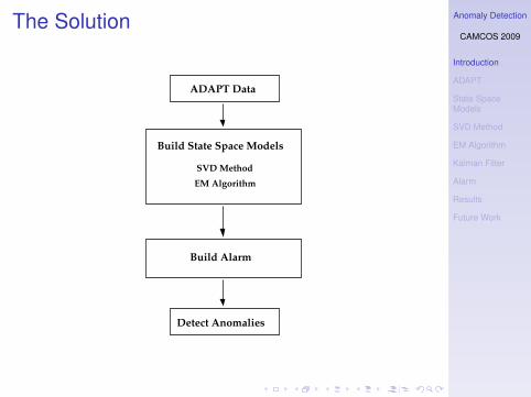
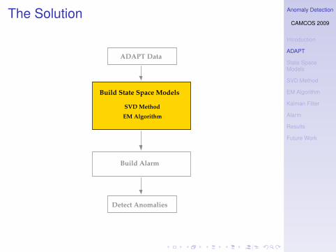
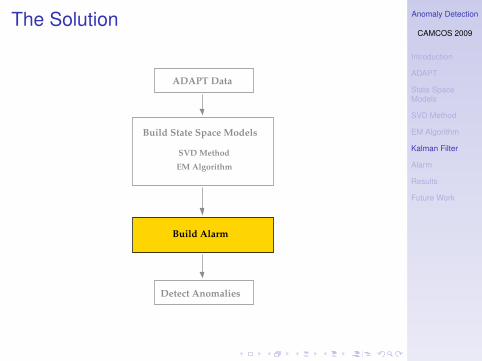
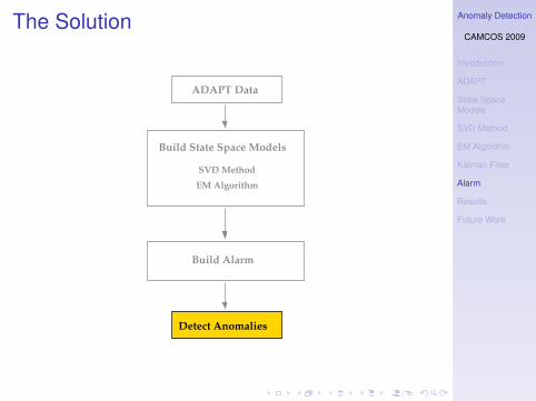
The Solution
Detect Anomalies
Build State Space Models
SVD Method
EM Algorithm
ADAPT Data
Build Alarm

Anomaly Detection
CAMCOS 2009
Introduction
ADAPT
State SpaceModels
SVD Method
EM Algorithm
Kalman Filter
Alarm
Results
Future Work
The Solution
ADAPT Data
EM Algorithm
SVD Method
Build State Space Models
Build Alarm
Detect Anomalies

Anomaly Detection
CAMCOS 2009
Introduction
ADAPT
State SpaceModels
SVD Method
EM Algorithm
Kalman Filter
Alarm
Results
Future Work
The System
Power Supply Controls Load Bank
Anomaly Detection
CAMCOS 2009
Introduction
ADAPT
State SpaceModels
SVD Method
EM Algorithm
Kalman Filter
Alarm
Results
Future Work
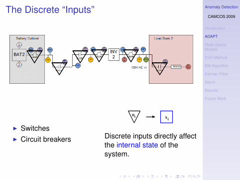
The Discrete “Inputs”
I SwitchesI Circuit breakers
t
ut x
Discrete inputs directly affectthe internal state of thesystem.

Anomaly Detection
CAMCOS 2009
Introduction
ADAPT
State SpaceModels
SVD Method
EM Algorithm
Kalman Filter
Alarm
Results
Future Work
The Continuous “Outputs”
I VoltageI CurrentI TemperatureI Phase angleI Speed/flow
t ytx
t
u
Continuous outputs areaffected by the internal stateof the system, as well as bythe inputs.

Anomaly Detection
CAMCOS 2009
Introduction
ADAPT
State SpaceModels
SVD Method
EM Algorithm
Kalman Filter
Alarm
Results
Future Work
The Data
Data collected fromexperiments
I Uniform time length
I Different switchesflipped at differenttimes
I 79 nominal data sets
I 154 faulty data sets

Anomaly Detection
CAMCOS 2009
Introduction
ADAPT
State SpaceModels
SVD Method
EM Algorithm
Kalman Filter
Alarm
Results
Future Work
Nominal Data
I 79 data setscollected with noerrors
I We used these tofigure out how thesystem actsnormally
Anomaly Detection
CAMCOS 2009
Introduction
ADAPT
State SpaceModels
SVD Method
EM Algorithm
Kalman Filter
Alarm
Results
Future Work
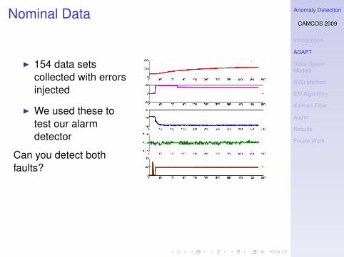
Nominal Data
I 154 data setscollected with errorsinjected
I We used these totest our alarmdetector
Can you detect bothfaults?
Anomaly Detection
CAMCOS 2009
Introduction
ADAPT
State SpaceModels
SVD Method
EM Algorithm
Kalman Filter
Alarm
Results
Future Work
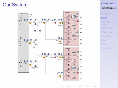
Our System

Anomaly Detection
CAMCOS 2009
Introduction
ADAPT
State SpaceModels
SVD Method
EM Algorithm
Kalman Filter
Alarm
Results
Future Work
Our System
Anomaly Detection
CAMCOS 2009
Introduction
ADAPT
State SpaceModels
SVD Method
EM Algorithm
Kalman Filter
Alarm
Results
Future Work
The Solution
ADAPT Data
EM Algorithm
SVD Method
Build State Space Models
Build Alarm
Detect Anomalies

Anomaly Detection
CAMCOS 2009
Introduction
ADAPT
State SpaceModels
SVD Method
EM Algorithm
Kalman Filter
Alarm
Results
Future Work
The ADAPT System
I Triangles around inputs
I Circles around outputs
Anomaly Detection
CAMCOS 2009
Introduction
ADAPT
State SpaceModels
SVD Method
EM Algorithm
Kalman Filter
Alarm
Results
Future Work
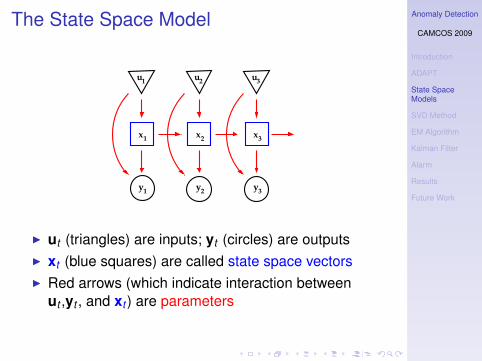
The State Space Model
y1
x x x1
u2
2
u1
3
u3
y2
y3
I ut (triangles) are inputs; yt (circles) are outputsI xt (blue squares) are called state space vectorsI Red arrows (which indicate interaction between
ut ,yt , and xt ) are parameters

Anomaly Detection
CAMCOS 2009
Introduction
ADAPT
State SpaceModels
SVD Method
EM Algorithm
Kalman Filter
Alarm
Results
Future Work
What We Know
y1
u2
u1
u3
y2
y3
I We do not know our xt
whitespacewhitespacewhitespace

Anomaly Detection
CAMCOS 2009
Introduction
ADAPT
State SpaceModels
SVD Method
EM Algorithm
Kalman Filter
Alarm
Results
Future Work
What We Know
y1
u2
u1
u3
y2
y3
I We do not know our xt
I We do not know our parameters
whitespacewhitespace

Anomaly Detection
CAMCOS 2009
Introduction
ADAPT
State SpaceModels
SVD Method
EM Algorithm
Kalman Filter
Alarm
Results
Future Work
The State Space Equations
xt = Axt−1 + But + wt
yt = Cxt + Dut + vt
whitespace
I Vectors ut are inputs
I Vectors yt are outputs
I Vectors xt are state space vectors
I Matrices A,B,C,D and vectors wt ,vt are parameters

Anomaly Detection
CAMCOS 2009
Introduction
ADAPT
State SpaceModels
SVD Method
EM Algorithm
Kalman Filter
Alarm
Results
Future Work
Problem Outline
I What is our state space dimension, dim(xt )? (SVDmethod)
I How do we find the parameters? (EM algorithm)
I How do we find our state space vectors xt? (KalmanFilter)
I How does this model detect an anomaly?

Anomaly Detection
CAMCOS 2009
Introduction
ADAPT
State SpaceModels
SVD Method
EM Algorithm
Kalman Filter
Alarm
Results
Future Work
The Solution
ADAPT Data
EM Algorithm
SVD Method
Build State Space Models
Build Alarm
Detect Anomalies
Anomaly Detection
CAMCOS 2009
Introduction
ADAPT
State SpaceModels
SVD Method
EM Algorithm
Kalman Filter
Alarm
Results
Future Work
State Space Dimension Estimation
I Problem: What is the dimension of the hidden statespace vector xt?
I To find dim xt , we use the singular valuedecomposition (SVD) method.

Anomaly Detection
CAMCOS 2009
Introduction
ADAPT
State SpaceModels
SVD Method
EM Algorithm
Kalman Filter
Alarm
Results
Future Work
SVD Method
I Formulate the Hankel matrixI The Hankel matrix describes the autocorrelations of
the input vectors ut and the output vectors yt .
I Compute singular values of the Hankel matrixI Singular values are non-negative numbers.
I In case of no noise, the number of nonzero singularvalues equals the state space dimension.

Anomaly Detection
CAMCOS 2009
Introduction
ADAPT
State SpaceModels
SVD Method
EM Algorithm
Kalman Filter
Alarm
Results
Future Work
Reasons to Use SVD Method
We decide to use the SVD method because:I It does not rely on parameters A,B,C,D.
I It is computationally fast.
The SVD method is based on a theorem due toKronecker’s contributions.

Anomaly Detection
CAMCOS 2009
Introduction
ADAPT
State SpaceModels
SVD Method
EM Algorithm
Kalman Filter
Alarm
Results
Future Work
Theorem
In the absence of error, the rank of the Hankel matrix isequal to the state space dimension.
Kronecker 1823-1891
I Rank of Hankel matrix = number of non-zero singularvalues.
I State space dimension = dim(xt ).
Anomaly Detection
CAMCOS 2009
Introduction
ADAPT
State SpaceModels
SVD Method
EM Algorithm
Kalman Filter
Alarm
Results
Future Work
Simulation
I We validate our SVD method with simulated data.
I Simulated data has dim(xt ) = 5.
I We expect our result to have the same state spacedimension.

Anomaly Detection
CAMCOS 2009
Introduction
ADAPT
State SpaceModels
SVD Method
EM Algorithm
Kalman Filter
Alarm
Results
Future Work
Simulation Result

Anomaly Detection
CAMCOS 2009
Introduction
ADAPT
State SpaceModels
SVD Method
EM Algorithm
Kalman Filter
Alarm
Results
Future Work
Real ADAPT
I Real ADAPT data has noise, so it is difficult todetermine the precise state space dimension.
I dim(xt ) can be any positive integer; the optimaldimension is unknown
I Too few versus too many dimensionsI Choosing dimension too small–ignores available
informationI Choosing dimension too large–unnecessarily
complicates system

Anomaly Detection
CAMCOS 2009
Introduction
ADAPT
State SpaceModels
SVD Method
EM Algorithm
Kalman Filter
Alarm
Results
Future Work
Real ADAPT Result

Anomaly Detection
CAMCOS 2009
Introduction
ADAPT
State SpaceModels
SVD Method
EM Algorithm
Kalman Filter
Alarm
Results
Future Work
The Solution
ADAPT Data
EM Algorithm
SVD Method
Build State Space Models
Build Alarm
Detect Anomalies
Anomaly Detection
CAMCOS 2009
Introduction
ADAPT
State SpaceModels
SVD Method
EM Algorithm
Kalman Filter
Alarm
Results
Future Work
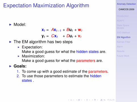
Expectation Maximization Algorithm
I Model:xt = Axt−1 + But + wt
yt = Cxt + Dut + vt
I The EM algorithm has two stepsI Expectation:
Make a good guess for what the hidden states are.I Maximization:
Make a good guess for what the parameters are.I Goals:
1. To come up with a good estimate of the parameters.2. To use those parameters to estimate the hidden
states .

Anomaly Detection
CAMCOS 2009
Introduction
ADAPT
State SpaceModels
SVD Method
EM Algorithm
Kalman Filter
Alarm
Results
Future Work
EM Algorithm Variables
I Known Quantities (u,y)player statistics, game results
I Hidden States (x)how the game is actually going
I Parameters how the players’ abilities interact

Anomaly Detection
CAMCOS 2009
Introduction
ADAPT
State SpaceModels
SVD Method
EM Algorithm
Kalman Filter
Alarm
Results
Future Work
Running the Algorithm
Problem:I Without knowing what the hidden states are, we
cannot estimate the parameters.I Without knowing what the parameters are, we cannot
estimate the hidden states.
Solution:I Hidden States
Kalman FilterI Parameters
Maximum LikelihoodEstimation

Anomaly Detection
CAMCOS 2009
Introduction
ADAPT
State SpaceModels
SVD Method
EM Algorithm
Kalman Filter
Alarm
Results
Future Work
Maximum Likelihood Estimation
xt = Axt−1 + But + wt
yt = Cxt + Dut + vt
I Given that we have some observations (the y ’s),what are the parameters that would make those y ’smost likely to have occurred?
I Under reasonable assumptions, we can construct asingle function of the parameters that includes all ofthe data.
I We call this function L the likelihood function, and itis essentially a measure of how well the model fits.

Anomaly Detection
CAMCOS 2009
Introduction
ADAPT
State SpaceModels
SVD Method
EM Algorithm
Kalman Filter
Alarm
Results
Future Work
The Likelihood Function
L = f (x0)T∏
t=1
f (x t |ut ,x t−1)T∏
t=1
f (y t |ut ,x t )
I We claim that maximizing this function will give us aset of parameters that would make our data “mostlikely” to have occurred.
I L is a function of 4534 unknown variables (notcounting the hidden states).
I There are two ways to maximize L:I Gradient ascentI Solve it analytically

Anomaly Detection
CAMCOS 2009
Introduction
ADAPT
State SpaceModels
SVD Method
EM Algorithm
Kalman Filter
Alarm
Results
Future Work
Maximum Likelihood Estimation
I Some functions are easy to maximize:
I Some are a little trickier:

Anomaly Detection
CAMCOS 2009
Introduction
ADAPT
State SpaceModels
SVD Method
EM Algorithm
Kalman Filter
Alarm
Results
Future Work
Iterate
I Use a guess for the parameters, along with a guessfor the first hidden state (x0), to estimate all of the x ’susing the Kalman Filter).
I Use that data to improve our estimation of theparameters, and repeat.
One we are satisfied that we have estimated theparameters as well as we can, we can ask the importantquestion:
I Given that we have a reasonable idea of what toexpect, what kind of data would be unusual?

Anomaly Detection
CAMCOS 2009
Introduction
ADAPT
State SpaceModels
SVD Method
EM Algorithm
Kalman Filter
Alarm
Results
Future Work
The Solution
ADAPT Data
EM Algorithm
SVD Method
Build State Space Models
Build Alarm
Detect Anomalies

Anomaly Detection
CAMCOS 2009
Introduction
ADAPT
State SpaceModels
SVD Method
EM Algorithm
Kalman Filter
Alarm
Results
Future Work
Need to Filter Noise
Practical Problem: Getting Apollomissions safely to the moon and back.
I Abstract Problem: For each time t , given pastobservations y t−1, . . . , y1 make prediction y t−1
t ofpresent y t and of the variance (average uncertainty)between predicted and actual observation.
I At each time some noise with known variancecorrupts both observation and hidden state
I Goal: filter, compensate, for accumulated noiseI Rudolph Kalman presented solution, Kalman filter
(1960), extended by NASA Ames for Apollo

Anomaly Detection
CAMCOS 2009
Introduction
ADAPT
State SpaceModels
SVD Method
EM Algorithm
Kalman Filter
Alarm
Results
Future Work
Filtering Visually a Graph for Increasing Time
0 2 4 6 8 10 12 14 16 18time
observedexpected
I Predict expected values left-to-right, time t predictionfrom past t − 1, t − 2, . . . ,2,1.
I Be skeptical of extreme values, because values atprevious times do not support—value time 10
I Increase skepticism as noise accumulates with time.I Draw expected value curve “in middle” of observed.

Anomaly Detection
CAMCOS 2009
Introduction
ADAPT
State SpaceModels
SVD Method
EM Algorithm
Kalman Filter
Alarm
Results
Future Work
Hidden State Estimated from Observations
Image: Moment ofdecision at MissionControl Center forwhether Apollo 16 shouldland on the Moon
I Hidden state x t , such as position, determines all.I Each time t , predict hidden state x t−1
t from pastt − 1, t − 2, . . . ,2,1, then using model predictobservation y t−1
t at next time t
I Prediction error y t − y t−1t of observation compared
to its variance used to correct prediction of hiddenstate x t
t , now hidden state given observationsincluding that at current time t and of past.

Anomaly Detection
CAMCOS 2009
Introduction
ADAPT
State SpaceModels
SVD Method
EM Algorithm
Kalman Filter
Alarm
Results
Future Work
Kalman Filter Can Estimate Uncertainty
0 2 4 6 8 10 12 14 16 18 206
7
8
9
10
11
12
13
14
15
time
y
Kalman Filter Applied to 1D Output
observedfilteredupper boundlower bound
I Data generated from “nice” model stays withinuncertainty bounds in green after Kalman filtering
I Bounds obtained through Mahalanobis distance c2t ,
error scaled by predicted variance Σt at time t
c2t = (yt − yt−1
t )T Σ−1t (yt − yt−1
t )

Anomaly Detection
CAMCOS 2009
Introduction
ADAPT
State SpaceModels
SVD Method
EM Algorithm
Kalman Filter
Alarm
Results
Future Work
Using Many Data Sets for Detection
I Are given many sets of data without anomalyI Using EM algorithm each data set has its own state
space modelI Given another data set, for each previous model, can
use Kalman filter to make predictions both ofvalues and of Mahalanobis distances c2
tI Since assumed same physical system, ADAPT
testbed, do data sets give models that say somethingabout different data from same system? Yes, so wecan compute in advance.
I Using information from many data sets:I Use c2
t as statisticsI Given these c2
t statistics varying in time, what isanomalous?
Anomaly Detection
CAMCOS 2009
Introduction
ADAPT
State SpaceModels
SVD Method
EM Algorithm
Kalman Filter
Alarm
Results
Future Work
The Solution
ADAPT Data
EM Algorithm
SVD Method
Build State Space Models
Build Alarm
Detect Anomalies

Anomaly Detection
CAMCOS 2009
Introduction
ADAPT
State SpaceModels
SVD Method
EM Algorithm
Kalman Filter
Alarm
Results
Future Work
Building the Alarm
I Methods: SVD and EM algorithm gave us the modelfor ADAPT system.
xt = Axt−1 + But + wt
yt = Cxt + Dut + vt
I Model enables us to generate expectedobservations, y’s.
I Expected y’s form an ellipsoid = (mean, spread ofexpected y’s).
I Compare real-time readings yt to the expectedobservations yt within the ellipsoid.

Anomaly Detection
CAMCOS 2009
Introduction
ADAPT
State SpaceModels
SVD Method
EM Algorithm
Kalman Filter
Alarm
Results
Future Work
Outputs / Sensor Readings
−2 −1.5 −1 −0.5 0 0.5 1 1.5 2 2.5−3
−2
−1
0
1
2
3
Observations
Goal:I Single out outliers = find dots outside the ellipsoid

Anomaly Detection
CAMCOS 2009
Introduction
ADAPT
State SpaceModels
SVD Method
EM Algorithm
Kalman Filter
Alarm
Results
Future Work
Numbers for Vectors
I Our sensors readings are vectors of a highdimension; dim yt = 50
I Appropriate metric to determine the multivariateoutliers is a Mahalanobis distance
I To each observation vector at each time step we areassigning a number, yt 7→ c2
t
I c2t is a Mahalanobis distance that measures how far
our actual observation is from the expected one
−2 −1.5 −1 −0.5 0 0.5 1 1.5 2 2.5−3
−2
−1
0
1
2
3
Observat ions
Anomaly Detection
CAMCOS 2009
Introduction
ADAPT
State SpaceModels
SVD Method
EM Algorithm
Kalman Filter
Alarm
Results
Future Work
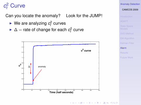
c2t Curve
Can you locate the anomaly? Look for the JUMP!
I We are analyzing c2t curves
I ∆ = rate of change for each c2t curve
0 50 100 150 200 250 300 350 400 4500.98
1
1.02
1.04
1.06
1.08
1.1
1.12
1.14
1.16
Time (half seconds)
c2
c2 curve
anomalyΔ

Anomaly Detection
CAMCOS 2009
Introduction
ADAPT
State SpaceModels
SVD Method
EM Algorithm
Kalman Filter
Alarm
Results
Future Work
Anomaly Detection
I 74 nominal data sets = 74 "experts"I Our "Alarm" relies on many of the 74 c2
t curves
0 50 100 150 200 250 300 350 400 4500
0.5
1
1.5
2
2.5
3
3.5
4
4.5x 10⁴
Time (half seconds)
c2
c2 curves

Anomaly Detection
CAMCOS 2009
Introduction
ADAPT
State SpaceModels
SVD Method
EM Algorithm
Kalman Filter
Alarm
Results
Future Work
Thresholds on c2t
1. ∆ = Rate of change in each c2t curve
∆ suddenly increases⇒ "Alarm"
2. # of Experts saying "Alarm"Don’t trust just one "expert" screamingAlarm!
Both rates will be used to adjust the sensitivity of ourdetector.
Anomaly Detection
CAMCOS 2009
Introduction
ADAPT
State SpaceModels
SVD Method
EM Algorithm
Kalman Filter
Alarm
Results
Future Work
The Solution
ADAPT Data
EM Algorithm
SVD Method
Build State Space Models
Build Alarm
Detect Anomalies

Anomaly Detection
CAMCOS 2009
Introduction
ADAPT
State SpaceModels
SVD Method
EM Algorithm
Kalman Filter
Alarm
Results
Future Work
Expectations for our Anomaly Detector
I We want:I To detect faults accurately.
I A low False Positive Rate: a low number of falsealarms.
I A low False Negative Rate: a low number of missedfaults.
I To detect anomalies within a few seconds of the faultoccuring.
I To have a fast computation time (real-time).
I To use as little memory as possible.

Anomaly Detection
CAMCOS 2009
Introduction
ADAPT
State SpaceModels
SVD Method
EM Algorithm
Kalman Filter
Alarm
Results
Future Work
Receiver Operating Characteristic (ROC)I Each point along the curve is a True Positive Rate
(TPR) and False Positive Rate (FPR) for a chosenthreshold.
I A true positive is when our method detects a faultwhen a fault has occured in the system.
I A false positive is when our method detects a faultwhen no fault has occured in the system.
0 0.1 0.2 0.3 0.4 0.5 0.6 0.7 0.8 0.9 10
0.1
0.2
0.3
0.4
0.5
0.6
0.7
0.8
0.9
1ROC Expert % = 4
False Positive Rate
Tru
e P
ositi
ve R
ate
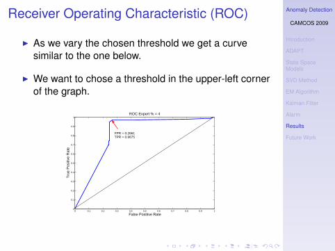
FPR = 0.2661TPR = 0.9675
Anomaly Detection
CAMCOS 2009
Introduction
ADAPT
State SpaceModels
SVD Method
EM Algorithm
Kalman Filter
Alarm
Results
Future Work
Receiver Operating Characteristic (ROC)
I As we vary the chosen threshold we get a curvesimilar to the one below.
I We want to chose a threshold in the upper-left cornerof the graph.
0 0.1 0.2 0.3 0.4 0.5 0.6 0.7 0.8 0.9 10
0.1
0.2
0.3
0.4
0.5
0.6
0.7
0.8
0.9
1ROC Expert % = 4
False Positive Rate
Tru
e P
ositi
ve R
ate
FPR = 0.2661TPR = 0.9675

Anomaly Detection
CAMCOS 2009
Introduction
ADAPT
State SpaceModels
SVD Method
EM Algorithm
Kalman Filter
Alarm
Results
Future Work
Our Results
0 0.1 0.2 0.3 0.4 0.5 0.6 0.7 0.8 0.9 10
0.1
0.2
0.3
0.4
0.5
0.6
0.7
0.8
0.9
1ROC Expert % = 4
False Positive Rate
Tru
e P
ositi
ve R
ate
FPR = 0.2661TPR = 0.9675
I This gives us a True Positive Rate of 0.9675.
I This gives us a False Positive Rate of 0.2661.
I On average, we are able to detect anomalies within5.85 seconds from the time the actual fault occured.

Anomaly Detection
CAMCOS 2009
Introduction
ADAPT
State SpaceModels
SVD Method
EM Algorithm
Kalman Filter
Alarm
Results
Future Work
Comparing to the DX Competition
I We follow the DX competition rules to the letterI Using only 34 nominal training sets on 120
competition files.I Files are counted as either false positives or false
negatives but not both.
False False AveragePositive Negative Detection
Team Rate Rate TimeLinköping University 0.5417 0.0972 3.490Canberra Research Lab 0.5106 0.0959 30.742Integra Software 0.8143 0.2400 14.099Carnegie Mellon / NASA 0.0732 0.1392 5.981UCSC / Perot Systems 0.0000 0.3000 17.610Stanford 0.3256 0.0519 3.946CAMCOS 0.3000 0.2125 5.903

Anomaly Detection
CAMCOS 2009
Introduction
ADAPT
State SpaceModels
SVD Method
EM Algorithm
Kalman Filter
Alarm
Results
Future Work
Future Work
I Instead of using the ellipsoid as our bound for y t , findthe closed form for the distribution of y t to generate aconfidence interval.
I This interval should give us a better bound on thevalues of y t and thus a better way of detectingoutliers.
I Any y t that is outside this confidence interval wouldbe considered an anomaly.
I This in turn would hopefully lead to us to achieve ahigher rate of detection accuracy.

Anomaly Detection
CAMCOS 2009
Introduction
ADAPT
State SpaceModels
SVD Method
EM Algorithm
Kalman Filter
Alarm
Results
Future Work
Future Work
I The next issue we would like to tackle is isolating theanomalies.
I Not only do we want to detect a fault accurately, butwe want to know where the fault is in the system.
I Once a fault is isolated then it is easier to find asolution to the problem and figure out what was thecause of the fault.

Anomaly Detection
CAMCOS 2009
Introduction
ADAPT
State SpaceModels
SVD Method
EM Algorithm
Kalman Filter
Alarm
Results
Future Work
Thank You
Thank You!

Anomaly Detection
CAMCOS 2009
Introduction
ADAPT
State SpaceModels
SVD Method
EM Algorithm
Kalman Filter
Alarm
Results
Future Work
LUNCH
��
��������������
Library
King
We Are Here
4th
Stre
et
10
th S
tree
t
San Fernando Street
Flames
Student Union
*

Anomaly Detection
CAMCOS 2009
AppendixAdditional Material HankelMatrix
EM Algorithm: AdditionalMaterial
Additional Material onKalman Filter
Kalman Filter Additional
Alarm Additional MaterialAppendixAdditional Material Hankel MatrixEM Algorithm: Additional MaterialAdditional Material on Kalman FilterKalman Filter AdditionalAlarm Additional Material
Anomaly Detection
CAMCOS 2009
AppendixAdditional Material HankelMatrix
EM Algorithm: AdditionalMaterial
Additional Material onKalman Filter
Kalman Filter Additional
Alarm Additional Material
Hankel Matrix
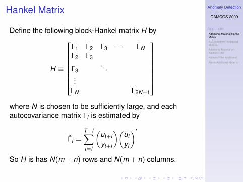
Define the following block-Hankel matrix H by
H ≡
Γ1 Γ2 Γ3 · · · ΓNΓ2 Γ3
Γ3. . .
...ΓN Γ2N−1
where N is chosen to be sufficiently large, and eachautocovariance matrix Γl is estimated by
Γl =T−l∑t=l
(ut+l
yt+l
)(ut
yt
)′
So H is has N(m + n) rows and N(m + n) columns.

Anomaly Detection
CAMCOS 2009
AppendixAdditional Material HankelMatrix
EM Algorithm: AdditionalMaterial
Additional Material onKalman Filter
Kalman Filter Additional
Alarm Additional Material
Assumptions
To use maximum likelihood estimation, we need to maketwo important assumptions about the data, which wehope conform to some extent with reality:
I That each timestep is independent of the previoustimesteps. We assume that each timestep containsall of the information from all previous timesteps.
I That we know how the data is distributed, even if wedon’t know the parameters of that distribution.
If we make these assumptions, each piece of data has itsown distribution (density function), and we can multiplythese together to get a new pdf, which we can then viewas a function of the parameters, not of the data.

Anomaly Detection
CAMCOS 2009
AppendixAdditional Material HankelMatrix
EM Algorithm: AdditionalMaterial
Additional Material onKalman Filter
Kalman Filter Additional
Alarm Additional Material
The Good News
If we begin with a guess, we can improve that guess until(hopefully) our guess mutates into something like thetruth.

Anomaly Detection
CAMCOS 2009
AppendixAdditional Material HankelMatrix
EM Algorithm: AdditionalMaterial
Additional Material onKalman Filter
Kalman Filter Additional
Alarm Additional Material
Parameters and Initialization
DefinitionLet parameters Θ be
Θ = {E [x0] ,V (x0),At ,Bt ,C t ,Dt ,V (w t ),V (v t )}∞t=1
Let F (Θ) stand for being a function of Θ, and F (Θ,Zs)stand for being a function of both Θ and Zs.
DefinitionLet x0
0 = E [x0] and V(εx0
0
)= V (x0), all F (Θ).

Anomaly Detection
CAMCOS 2009
AppendixAdditional Material HankelMatrix
EM Algorithm: AdditionalMaterial
Additional Material onKalman Filter
Kalman Filter Additional
Alarm Additional Material
Forward Recursion
TheoremIf x t−1
t−1 is F (Θ,Zt−1) and V(εx t−1
t−1
)is F (Θ), then
I covariance matrices are F (Θ)
V(εx t−1
t
); V
(εy t−1
t
); V
(εx t
t)
I x t−1t and y t−1
t are F (Θ,Zt−1)
I x tt is F (Θ,Zt ).
TheoremZt and Θ give real non-negative numbers det V
(εy t−1
t
)and
(εy t−1
t
)TV(εy t−1
t
)−1εy t−1
t .

Anomaly Detection
CAMCOS 2009
AppendixAdditional Material HankelMatrix
EM Algorithm: AdditionalMaterial
Additional Material onKalman Filter
Kalman Filter Additional
Alarm Additional Material
Intermediate Estimates
Theorem
x t−1t = At x t−1
t−1 + Btut (1)
y t−1t = C t x t−1
t + Dtut (2)
εy t−1t = y t − y t−1
t (3)
εx t−1t = Atεx t−1
t−1 + w t
εy t−1t = C tεx t−1
t + v t .
Proof.w t ⊥ Zt−1; v t ⊥ Zt−1

Anomaly Detection
CAMCOS 2009
AppendixAdditional Material HankelMatrix
EM Algorithm: AdditionalMaterial
Additional Material onKalman Filter
Kalman Filter Additional
Alarm Additional Material
Intermediate CovariancesTheorem
V(εx t−1
t
)= AtV
(εx t−1
t−1
)AT
t + V (w t ) (4)
V(εy t−1
t
)= C tV
(εx t−1
t
)CT
t + V (v t ) (5)
Σ(εx t−1
t , εy t−1t
)= V
(εx t−1
t
)CT
t (6)
Proof.Cross-covariances are 0 since
w t ⊥ εx t−1t−1
v t ⊥ εx t−1t−1
v t ⊥ w t

Anomaly Detection
CAMCOS 2009
AppendixAdditional Material HankelMatrix
EM Algorithm: AdditionalMaterial
Additional Material onKalman Filter
Kalman Filter Additional
Alarm Additional Material
Projection Theorem
To find the projection of x t on Zt , first project x t ontosubspace Zt−1 ⊂ Zt . Then project remainder εx t−1
t onnew knowledge εy t−1
t ∈ Zt since εy t−1t ⊥ Zt−1
Theorem
x tt = x t−1
t + K tεy t−1t (7)
where
K t = Σ(εx t−1
t , εy t−1t
)V(εy t−1
t
)−1(8)
is called the Kalman gain, K t = F (Θ).
Anomaly Detection
CAMCOS 2009
AppendixAdditional Material HankelMatrix
EM Algorithm: AdditionalMaterial
Additional Material onKalman Filter
Kalman Filter Additional
Alarm Additional Material
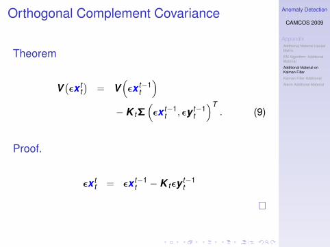
Orthogonal Complement Covariance
Theorem
V(εx t
t)
= V(εx t−1
t
)− K tΣ
(εx t−1
t , εy t−1t
)T. (9)
Proof.
εx tt = εx t−1
t − K tεy t−1t

Anomaly Detection
CAMCOS 2009
AppendixAdditional Material HankelMatrix
EM Algorithm: AdditionalMaterial
Additional Material onKalman Filter
Kalman Filter Additional
Alarm Additional Material
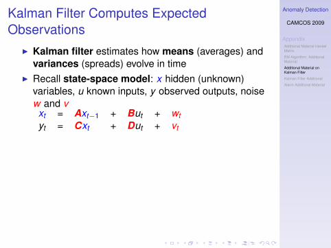
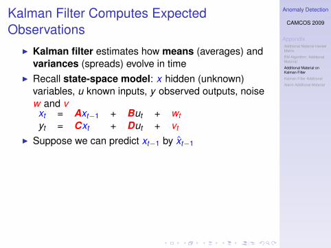
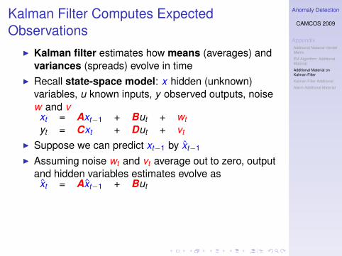
Kalman Filter Computes ExpectedObservations
I Kalman filter estimates how means (averages) andvariances (spreads) evolve in time
I Recall state-space model: x hidden (unknown)variables, u known inputs, y observed outputs, noisew and vxt = Axt−1 + But + wtyt = Cxt + Dut + vt
I Suppose we can predict xt−1 by xt−1
I Assuming noise wt and vt average out to zero, outputand hidden variables estimates evolve asxt = Axt−1 + But
yt = Cxt + Dut
I Have estimates of averages, can estimate errors ∆of form y − y = y − (Ax − Bu) orx − x = x − (Cx − Du).
Anomaly Detection
CAMCOS 2009
AppendixAdditional Material HankelMatrix
EM Algorithm: AdditionalMaterial
Additional Material onKalman Filter
Kalman Filter Additional
Alarm Additional Material
Kalman Filter Computes ExpectedObservations
I Kalman filter estimates how means (averages) andvariances (spreads) evolve in time
I Recall state-space model: x hidden (unknown)variables, u known inputs, y observed outputs, noisew and vxt = Axt−1 + But + wtyt = Cxt + Dut + vt
I Suppose we can predict xt−1 by xt−1
I Assuming noise wt and vt average out to zero, outputand hidden variables estimates evolve asxt = Axt−1 + But
yt = Cxt + Dut
I Have estimates of averages, can estimate errors ∆of form y − y = y − (Ax − Bu) orx − x = x − (Cx − Du).

Anomaly Detection
CAMCOS 2009
AppendixAdditional Material HankelMatrix
EM Algorithm: AdditionalMaterial
Additional Material onKalman Filter
Kalman Filter Additional
Alarm Additional Material
Kalman Filter Computes ExpectedObservations
I Kalman filter estimates how means (averages) andvariances (spreads) evolve in time
I Recall state-space model: x hidden (unknown)variables, u known inputs, y observed outputs, noisew and vxt = Axt−1 + But + wtyt = Cxt + Dut + vt
I Suppose we can predict xt−1 by xt−1
I Assuming noise wt and vt average out to zero, outputand hidden variables estimates evolve asxt = Axt−1 + Butyt = Cxt + Dut
I Have estimates of averages, can estimate errors ∆of form y − y = y − (Ax − Bu) orx − x = x − (Cx − Du).

Anomaly Detection
CAMCOS 2009
AppendixAdditional Material HankelMatrix
EM Algorithm: AdditionalMaterial
Additional Material onKalman Filter
Kalman Filter Additional
Alarm Additional Material
Kalman Filter Estimates Hidden Variables
y1
x x x1
u2
2
u1
3
u3
y2
y3
I Kalman filter estimates how means (averages) ofthe hidden variables xt and their variances(spreads) evolve in time
Anomaly Detection
CAMCOS 2009
AppendixAdditional Material HankelMatrix
EM Algorithm: AdditionalMaterial
Additional Material onKalman Filter
Kalman Filter Additional
Alarm Additional Material
MLE, Kalman Filter, Linear Algebra
I Assume probability density is (multivariable version)normal
f (w) =1√2π
1√σ2
exp(−1
21|σ2|
∆2)
where ∆ is an error and σ2 is the variance of noise
I Observe ∆ is function of model parameters A,B...I Iterate until f somehow “converges”
1. Fix model parameters A,B..., use Kalman filter toestimate ∆s.
2. Fix ∆s, use MLE to find model parameters A,B...that maximize probability density (now calledlikelihood function)
I Under all these assumptions, matrix algebra cansolve both Kalman filter estimates and MLE

Anomaly Detection
CAMCOS 2009
AppendixAdditional Material HankelMatrix
EM Algorithm: AdditionalMaterial
Additional Material onKalman Filter
Kalman Filter Additional
Alarm Additional Material
MLE, Kalman Filter, Linear Algebra
I Assume probability density is (multivariable version)normal
f (w) =1√2π
1√σ2
exp(−1
21|σ2|
∆2)
where ∆ is an error and σ2 is the variance of noiseI Observe ∆ is function of model parameters A,B...
I Iterate until f somehow “converges”
1. Fix model parameters A,B..., use Kalman filter toestimate ∆s.
2. Fix ∆s, use MLE to find model parameters A,B...that maximize probability density (now calledlikelihood function)
I Under all these assumptions, matrix algebra cansolve both Kalman filter estimates and MLE

Anomaly Detection
CAMCOS 2009
AppendixAdditional Material HankelMatrix
EM Algorithm: AdditionalMaterial
Additional Material onKalman Filter
Kalman Filter Additional
Alarm Additional Material
MLE, Kalman Filter, Linear Algebra
I Assume probability density is (multivariable version)normal
f (w) =1√2π
1√σ2
exp(−1
21|σ2|
∆2)
where ∆ is an error and σ2 is the variance of noiseI Observe ∆ is function of model parameters A,B...I Iterate until f somehow “converges”
1. Fix model parameters A,B..., use Kalman filter toestimate ∆s.
2. Fix ∆s, use MLE to find model parameters A,B...that maximize probability density (now calledlikelihood function)
I Under all these assumptions, matrix algebra cansolve both Kalman filter estimates and MLE

Anomaly Detection
CAMCOS 2009
AppendixAdditional Material HankelMatrix
EM Algorithm: AdditionalMaterial
Additional Material onKalman Filter
Kalman Filter Additional
Alarm Additional Material
Comparing ModelsI Recall state-space model:
xt = Axt−1 + But + wtyt = Cxt + Dut + vt
I If coordinate change–permuting hiddenvariables–same form model different parameters
I Want statistic valid with permutationI Kalman filter variance (spread) estimates Σt at time t
can scale output error ∆y to give such statistic
St = ∆yt Σ−1∆yt
I Kalman filter gives theoretical probability distributionProbt such that as time t varies, probability ofobserving this value of statistic or lower
Probt {z|z ≤ St}
should be “evenly distributed” from 0 to 1.

Anomaly Detection
CAMCOS 2009
AppendixAdditional Material HankelMatrix
EM Algorithm: AdditionalMaterial
Additional Material onKalman Filter
Kalman Filter Additional
Alarm Additional Material
Comparing ModelsI Recall state-space model:
xt = Axt−1 + But + wtyt = Cxt + Dut + vt
I If coordinate change–permuting hiddenvariables–same form model different parameters
I Want statistic valid with permutation
I Kalman filter variance (spread) estimates Σt at time tcan scale output error ∆y to give such statistic
St = ∆yt Σ−1∆yt
I Kalman filter gives theoretical probability distributionProbt such that as time t varies, probability ofobserving this value of statistic or lower
Probt {z|z ≤ St}
should be “evenly distributed” from 0 to 1.

Anomaly Detection
CAMCOS 2009
AppendixAdditional Material HankelMatrix
EM Algorithm: AdditionalMaterial
Additional Material onKalman Filter
Kalman Filter Additional
Alarm Additional Material
Comparing ModelsI Recall state-space model:
xt = Axt−1 + But + wtyt = Cxt + Dut + vt
I If coordinate change–permuting hiddenvariables–same form model different parameters
I Want statistic valid with permutationI Kalman filter variance (spread) estimates Σt at time t
can scale output error ∆y to give such statistic
St = ∆yt Σ−1∆yt
I Kalman filter gives theoretical probability distributionProbt such that as time t varies, probability ofobserving this value of statistic or lower
Probt {z|z ≤ St}
should be “evenly distributed” from 0 to 1.

Anomaly Detection
CAMCOS 2009
AppendixAdditional Material HankelMatrix
EM Algorithm: AdditionalMaterial
Additional Material onKalman Filter
Kalman Filter Additional
Alarm Additional Material
Comparing ModelsI Recall state-space model:
xt = Axt−1 + But + wtyt = Cxt + Dut + vt
I If coordinate change–permuting hiddenvariables–same form model different parameters
I Want statistic valid with permutationI Kalman filter variance (spread) estimates Σt at time t
can scale output error ∆y to give such statistic
St = ∆yt Σ−1∆yt
I Kalman filter gives theoretical probability distributionProbt such that as time t varies, probability ofobserving this value of statistic or lower
Probt {z|z ≤ St}
should be “evenly distributed” from 0 to 1.

Anomaly Detection
CAMCOS 2009
AppendixAdditional Material HankelMatrix
EM Algorithm: AdditionalMaterial
Additional Material onKalman Filter
Kalman Filter Additional
Alarm Additional Material
Validating With Model Following Assumptions
I Generate data fromstate-space system andnormal, independent,noise
I Estimate parametersusing MLE and Kalmanfilter
I Run Kalman filter usingthese parameters onsame data andcalculate statistics St
0 100 200 300 400 500 600 700 800 900 10000
0.1
0.2
0.3
0.4
0.5
0.6
0.7
0.8
0.9
1Multivariate normal state space system
time stepsC
umul
ativ
e D
istri
butio
n fo
r Sta
tistic
MLE and Kalman filter triesto attain picture for certainstatistic–evenly distributed

Anomaly Detection
CAMCOS 2009
AppendixAdditional Material HankelMatrix
EM Algorithm: AdditionalMaterial
Additional Material onKalman Filter
Kalman Filter Additional
Alarm Additional Material
Real Data, Different Data SetsI Estimate model from one data set, no faults,
calculate statistic for another data set, no faults, stillproblems–statistic just way too high
0 50 100 150 200 250 300 350 400 450 5000
0.2
0.4
0.6
0.8
1
1.2
1.4
1.6
1.8
2
time steps
Cum
ulat
ive
Dis
tribu
tion
for S
tatis
tic
Different ADAPT Files

Anomaly Detection
CAMCOS 2009
AppendixAdditional Material HankelMatrix
EM Algorithm: AdditionalMaterial
Additional Material onKalman Filter
Kalman Filter Additional
Alarm Additional Material
Validate Model on Real Data, Same Data SetI Use one ADAPT data set without anomalyI Estimate parameters using MLE and Kalman filter,
use parameters and Kalman filter back on samedata, calculate statistics {St}
I Somewhat similar results, except values close to 1during initial system startup
0 50 100 150 200 250 300 350 400 450 5000
0.1
0.2
0.3
0.4
0.5
0.6
0.7
0.8
0.9
1
time steps
Cum
ulat
ive
Dis
tribu
tion
for S
tatis
tic
Data Set Trained on Itself

Anomaly Detection
CAMCOS 2009
AppendixAdditional Material HankelMatrix
EM Algorithm: AdditionalMaterial
Additional Material onKalman Filter
Kalman Filter Additional
Alarm Additional Material
Mahalanobis distance
I Mahalanobis distance is based on correlationsbetween variables
I Mahalanobis distance of a n dim vector y from thegroup of expected observations with mean µy withcovariance matric Σ is defined as
c2t = (yt − µy )′Σ−1(yt − µy )
I for Σ = I the identity matrix, Mahalanobis distance =Euclidean distance

Anomaly Detection
CAMCOS 2009
AppendixAdditional Material HankelMatrix
EM Algorithm: AdditionalMaterial
Additional Material onKalman Filter
Kalman Filter Additional
Alarm Additional Material
References
Image of “Apollo 16 Command and Service Module Overthe Moon” http://grin.hq.nasa.gov/IMAGES/SMALL/GPN-2002-000069.jpgThe moment of decision at Mission Con-trol Center for whether Apollo 16 should land on the Moon,http://images.jsc.nasa.gov/search/search.cgi?searchpage=true&selections=AS16&browsepage=Go&hitsperpage=5&pageno=11