anomaly detection techniques for the condition monitoring ... · anomaly detection techniques for...

Anomaly Detection Techniques for the Condition Monitoring of

Tidal Turbines

Grant S. Galloway1, Victoria M. Catterson

2, Craig Love

3 and Andrew Robb

4

1, 2 Institute for Energy and Environment, Dept. EEE, University of Strathclyde, Glasgow, G1 1XW, UK

[email protected]

[email protected]

3, 4Andritz Hydro Hammerfest, Glasgow, G52 4RU, UK

ABSTRACT

Harnessing the power of currents from the sea bed, tidal

power has great potential to provide a means of renewable

energy generation more predictable than similar

technologies such as wind power. However, the nature of

the operating environment provides challenges, with

maintenance requiring a lift operation to gain access to the

turbine above water. Failures of system components can

therefore result in prolonged periods of downtime while

repairs are completed on the surface, removing the system’s

ability to produce electricity and damaging revenues. The

utilization of effective condition monitoring systems can

therefore prove particularly beneficial to this industry.

This paper explores the use of the CRISP-DM data mining

process model for identifying key trends within turbine

sensor data, to define the expected response of a tidal

turbine. Condition data from an operational 1 MW turbine,

installed off the coast of Orkney, Scotland, was used for this

study. The effectiveness of modeling techniques, including

curve fitting, Gaussian mixture modeling, and density

estimation are explored, using tidal turbine data in the

absence of faults. The paper shows how these models can

be used for anomaly detection of live turbine data, with

anomalies indicating the possible onset of a fault within the

system.

1. INTRODUCTION

Tidal power has great potential worldwide to be a major

contributing source of renewable energy. It is a European

target for 20% of energy generation to come from renewable

resources by 2020, as stated in the European Union

Committee 27th

Report of Session 2007-08. Within the UK

alone, tidal stream generation could potentially supply over

4 TWh per year within the next 5 to 10 years, with the

potential to reach up to 94 TWh per year with an installed

capacity of 36 GW (King & Tryfonas, 2009), around 26%

of the total electricity generated within the UK in 2013 (UK

Government electricity statistics). It is therefore clear that

tidal energy has the potential to provide a major contribution

to renewable sources of energy.

However, tidal power technology is in its infancy, and no

clear tidal turbine design has emerged as an industry

standard for extracting energy from tidal flow. The state of

the art in turbine design includes many horizontal and

vertical axis solutions, some with major structural and

operational variations (Aly & El-Hawary, 2011). However,

a common focus is the horizontal axis design, holding many

similarities with a standard wind turbine.

Maintenance on tidal turbines requires a lift operation to

access the turbine above sea-level. This can be a costly and

lengthy procedure, resulting in prolonged periods of

downtime. An effective condition monitoring system would

therefore be of great benefit to this industry, allowing the

health state of system components to be known, and

allowing maintenance to be scheduled efficiently.

Condition monitoring has already been well established for

the wind industry. However, despite similarities between

tidal and wind power turbine design, the operating

environment is vastly different. Water is over 800 times

denser than air and, despite slower flow rates (around 3 m/s

compared to around 15 m/s for offshore wind), tidal flow

has a much higher kinetic energy compared to wind flow

(Winter, 2011). This causes tidal turbines to operate with

higher torque and thrust loading, inducing increased stress

on the machine, particularly on the low speed stages of the

drive train. Additionally, the marine environment provides

other complications, such as corrosion and interaction with

plant and animal life. Furthermore, there is limited

historical data of failures from tidal turbines required to

Grant Galloway et al. This is an open-access article distributed under the terms of the Creative Commons Attribution 3.0 United States License,

which permits unrestricted use, distribution, and reproduction in any

medium, provided the original author and source are credited.

ANNUAL CONFERENCE OF THE PROGNOSTICS AND HEALTH MANAGEMENT SOCIETY 2014

2

implement condition monitoring techniques used as

standard in the wind industry.

This paper focuses on using anomaly detection techniques

for identifying developing faults within tidal turbines with

limited historical data. Using the CRISP-DM data mining

methodology (Wirth & Hipp, 2000), key relationships

between sensor data parameters from an operational tidal

turbine were identified, describing the normal response of

the turbine over variable operating conditions. These trends

were then defined using several modeling techniques,

allowing for deviations from expected data patterns to be

detected from live turbine data, alerting the operator to the

possible onset of a fault. The implementation of an

intelligent condition monitoring system is also discussed, to

integrate a number of seperate models together through a

decision system to assess the state of the turbine and its

components.

1.1. HS1000 Turbine

The data examined within this paper was sourced from the

Andritz Hydro Hammerfest HS1000 turbine (Figure 1). The

HS1000 is an operational tidal turbine with a rated power of

1 MW, deployed off the coast of Orkney, Scotland, as part

of the European Marine Energy Centre (EMEC).

Figure 1. The Andritz Hydro Hammerfest HS1000 tidal

turbine

The turbine has an open-blade horizontal axis design, fixed

to the seabed. Similar to a wind turbine, its drive train

consists of a gearbox connected to an induction generator,

translating tidal speeds of around 3.5 m/s to rotations

exceeding 1000 RPM within the generator. The turbine has

no yaw, with blades rotating in opposite directions in

response to upstream and downstream tides. Pitch control

of the blades is used to control the output power produced.

This paper will focus on data from the following sources:

Tri-axial generator vibration velocity

Gearbox vibration velocity

Bearing vibration velocity

Bearing displacement

Bearing temperature

Generator rotor speed

Output power

1.2. Data Mining

Data mining is the analysis of large data sets for knowledge

discovery. It involves the use of processing techniques,

involving statistical, machine learning and visualization

methods, to extract patterns and relationships hidden within

data parameters (Olson & Delen, 2008). Data mining has

been commonly used by banking and marketing firms, and

also within the medical field applied to vast amounts of

patient records for improved diagnosis and prediction

(Maimon & Rokach, 2005).

Within this study, data mining was used to discover trends

and relationships between parameters within initial datasets

from the HS1000 tidal turbine. A modeling stage then

defines the expected response of the turbine over its typical

range of operating conditions. By comparing live turbine

data to these models, anomaly detection is used to indicate a

change in the response of the system, indicating the possible

onset of a fault.

1.2.1. CRISP-DM

The CRISP-DM (Cross-Industry Standard Process for Data

Mining) process model was utilized for this study. This

model manages the data mining process as six key stages:

business understanding, data understanding, data

preparation, modeling, evaluation, and deployment (Wirth

& Hipp, 2000). These stages are shown in figure 2.

Figure 2. The CRISP-DM process model for data mining

(Wirth & Hipp, 2000)

Each stage of the CRISP-DM process model was employed

as follows:

Business Understanding – Understand the operating

environment of the turbine and how condition

monitoring may be used to assess turbine health.

Data Understanding – Use statistical analysis to identify

key parameters, relationships, and trends to learn the


3

response of sensor data over standard operating

conditions.

Data Preparation – Organize sensor data before

modeling, trending data and grouping by tidal cycle and

operating state of the turbine.

Modeling – Model key trends and relationships using

curve fitting, Gaussian mixture modeling and kernel

density estimation to define the response of data

parameters over varying operating conditions.

Evaluation – Evaluate the performance of each model,

using past operational data to train and test models for

anomaly detection.

Deployment – Compare live data to models and identify

deviations from expected behavior, integrating multiple

models together through an intelligent condition

monitoring system.

2. BUSINESS UNDERSTANDING

The business understanding phase of the CRISP-DM

process model involved an appreciation of the operating

environment and its effect on the expected response of the

turbine. The role of condition monitoring within the field

was also considered.

2.1. Condition Monitoring

The use of sensor data from turbine components (such as the

gearbox, generator, bearings, blades, etc) can allow the

onset of faults to be detected before they cause failure. This

enables an efficient maintenance strategy to be employed, as

maintenance can be scheduled to reflect to the known health

of system components.

Examples of previous research on condition monitoring for

tidal turbines includes:

A review of condition monitoring and prognostic

techniques applicable to tidal turbines (Wald,

Khoshgoftaar, Beaujean & Sloan, 2010).

Use of Failure Modes and Effects Analysis (FMEA) to

detect faults and failures within tidal turbines (Prickett,

Grosvenor, Byrne, Jones, Morris, O’Doherty &

O’Doherty, 2011).

Design of a dynamometer for simulating tidal turbine

bearing faults, and application of wavelet based

monitoring (Duhaney, Khoshgaftaar, Sloan, Alhalibi &

Beaujean, 2011).

Fatigue analysis of tidal turbine blades (Mahfuz &

Akram, 2011).

However, since tidal turbines have limited deployment,

there are few examples of condition monitoring systems

implemented in practice reported in the literature.

2.2. Turbine Operation

The EMEC test site in Orkney experiences a semi-diurnal

tide, with corresponding high and low tides each day.

Upstream and downstream tidal flow is experienced by the

HS1000 turbine in cycles between each high and low tide.

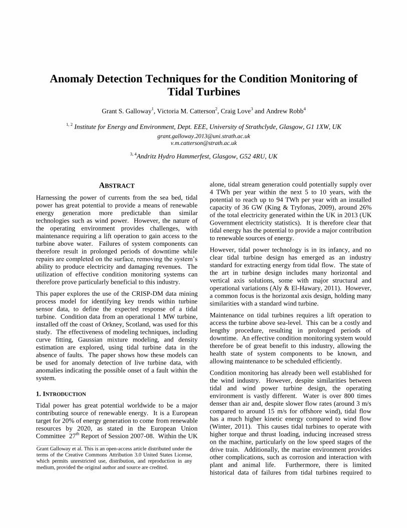
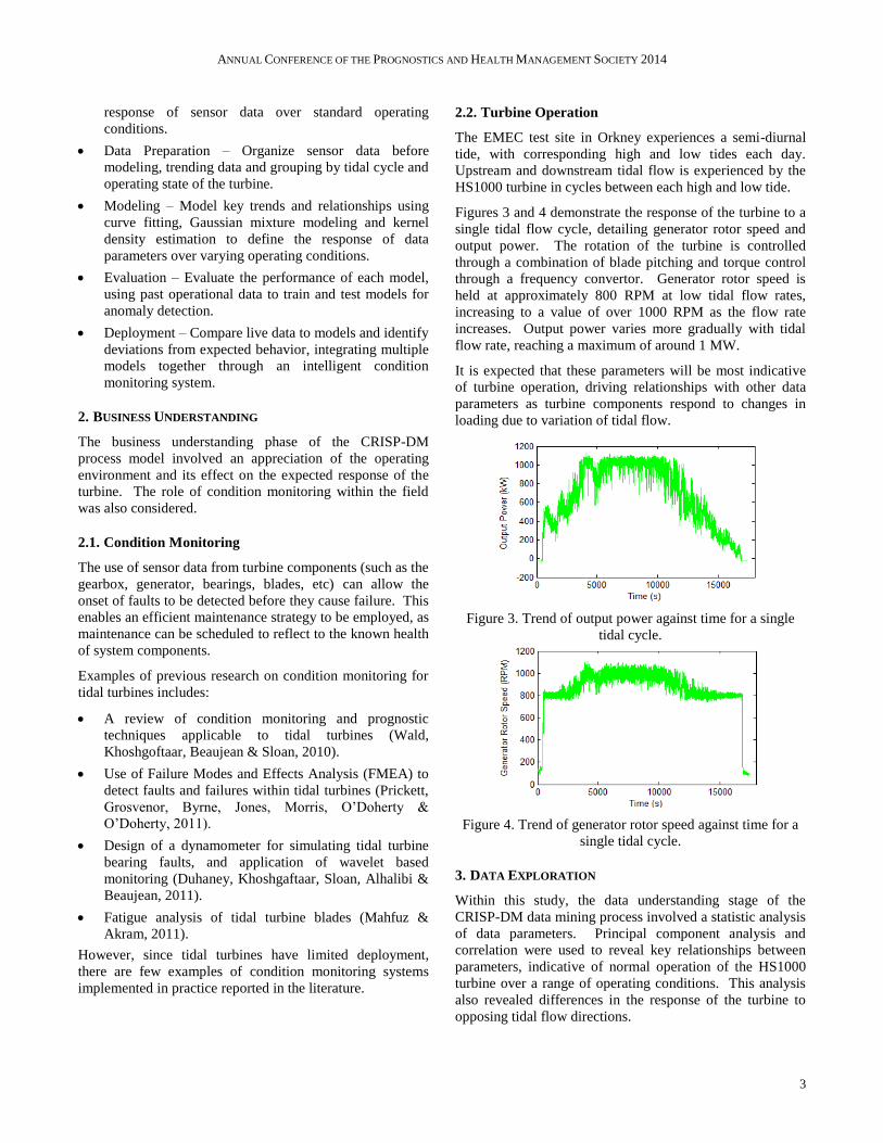
Figures 3 and 4 demonstrate the response of the turbine to a

single tidal flow cycle, detailing generator rotor speed and

output power. The rotation of the turbine is controlled

through a combination of blade pitching and torque control

through a frequency convertor. Generator rotor speed is

held at approximately 800 RPM at low tidal flow rates,

increasing to a value of over 1000 RPM as the flow rate

increases. Output power varies more gradually with tidal

flow rate, reaching a maximum of around 1 MW.

It is expected that these parameters will be most indicative

of turbine operation, driving relationships with other data

parameters as turbine components respond to changes in

loading due to variation of tidal flow.

Figure 3. Trend of output power against time for a single

tidal cycle.

Figure 4. Trend of generator rotor speed against time for a

single tidal cycle.

3. DATA EXPLORATION

Within this study, the data understanding stage of the

CRISP-DM data mining process involved a statistic analysis

of data parameters. Principal component analysis and

correlation were used to reveal key relationships between

parameters, indicative of normal operation of the HS1000

turbine over a range of operating conditions. This analysis

also revealed differences in the response of the turbine to

opposing tidal flow directions.


4

3.1. Principal Component Analysis

Principal component analysis (PCA) is a technique used to

extract and remove linear correlations from a set of

multivariate data (Pearson, 1901). This technique generates

a set of principal components, which are the uncorrelated

parameters underlying the observations within the data

(Abdi & Williams, 2010).

Components are a list of coefficients, representing a weight

for each input parameter, and an eigenvalue. Parameters

with high weightings are the highest contributors to

relationships within the data, and parameters with low

weighting contribute the least. A component’s eigenvalue is

representative of the significance of a component to the

data.

Results for this analysis returned components with high

coefficient weightings for output power and generator

rotation speed values, with high corresponding eigenvalues

(in the range of 1x103 to 1x10

5). This confirmed these

parameters were highly relevant within the data, driving

relationships between other data parameters.

3.2. Correlation

Correlation describes the statistical relationship between

two variables or data sets. This can be expressed via

Pearson’s correlation coefficient, which is a value

describing the linear dependence of two parameters

(Rodgers & Nicewander, 1988). This value ranges between

+1 (an ideal increasing linear relationship) and -1 (an ideal

decreasing linear relationship). Parameters with a

correlation coefficient of zero have no association to each

other.

Pearson’s correlation coefficient was calculated for every

pair of data parameters. High correlation was consistently

seen in output power and generator rotor speed parameters,

confirming these parameters are key to the response of other

sensor data parameters (in particular gearbox and generator

vibrations). Therefore, for the modeling stage of data

mining, all other data parameters (including vibration,

displacement and temperature readings from the gearbox,

generator and bearings) were trended against output power

and generator rotor speed. These relationships describe the

response of turbine components over a range of varying

operating conditions.

Comparison of these values also highlighted a change in

system response between upstream and downstream tidal

flows. This was expected as changes in tidal flow direction

alter the direction of loads on the turbine. As a result, for

the following stage of analysis, data was batched by tidal

cycle and categorized by tidal flow direction. Separate

models were then constructed to define the expected turbine

response for both tidal flow directions.

3.3. Visual Analysis

Visual analysis confirmed meaningful relationships were

generated by plotting data parameters against output power

and generator rotor speed.

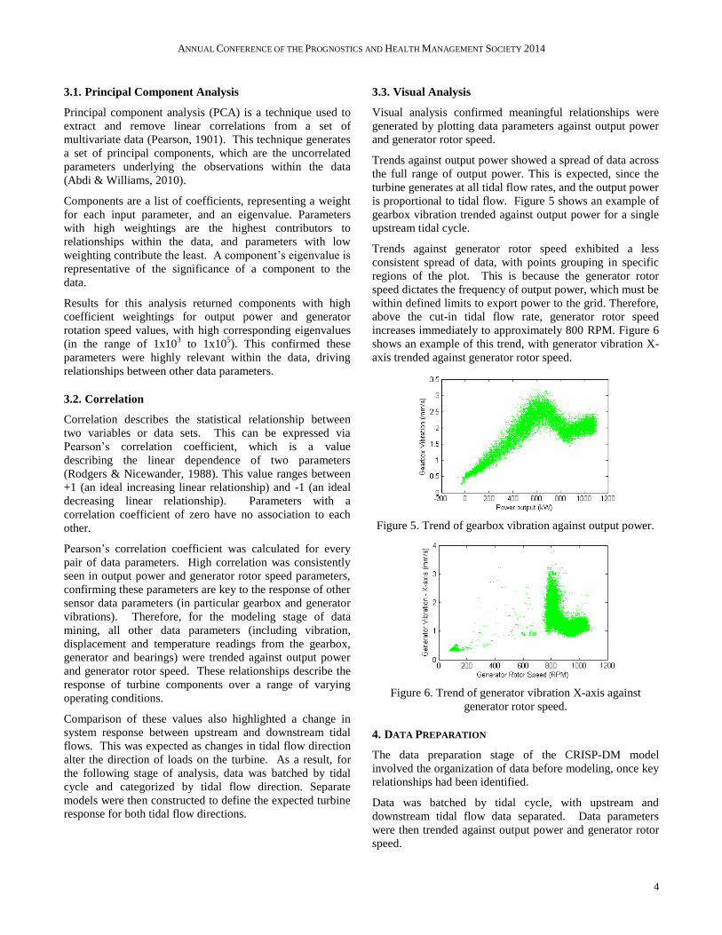
Trends against output power showed a spread of data across

the full range of output power. This is expected, since the

turbine generates at all tidal flow rates, and the output power

is proportional to tidal flow. Figure 5 shows an example of

gearbox vibration trended against output power for a single

upstream tidal cycle.

Trends against generator rotor speed exhibited a less

consistent spread of data, with points grouping in specific

regions of the plot. This is because the generator rotor

speed dictates the frequency of output power, which must be

within defined limits to export power to the grid. Therefore,

above the cut-in tidal flow rate, generator rotor speed

increases immediately to approximately 800 RPM. Figure 6

shows an example of this trend, with generator vibration X-

axis trended against generator rotor speed.

Figure 5. Trend of gearbox vibration against output power.

Figure 6. Trend of generator vibration X-axis against

generator rotor speed.

4. DATA PREPARATION

The data preparation stage of the CRISP-DM model

involved the organization of data before modeling, once key

relationships had been identified.

Data was batched by tidal cycle, with upstream and

downstream tidal flow data separated. Data parameters

were then trended against output power and generator rotor

speed.


5

Also at this stage, four key regions of data were defined, to

further segment data before models were constructed.

These regions were representative of the operating state of

the turbine, and defined using change point analysis (Killick

& Eckley, 2013) applied to the speed-power curve of the

turbine.

4.1. Change Point Analysis

Change point analysis is a technique used to find a series of

points within data parameters where changes in the data are

most significant. Change points are determined by

calculating a vector of the sum of differences between each

data point and the mean of all data points. The maximum or

minimum point on this vector will indicate the location of a

change point (Killick & Eckley, 2013). This process can be

repeated to find additional change points within each newly

identified region.

Four regions of operation were visible from the speed-

power curve (figure 7):

1. Start up and shut down region

2. Constant rotor speed region

3. Increasing rotor speed region

4. Turbine rotor speed and power limitation region

Figure 7 shows the result of change point analysis in

defining these operating state regions. Separating these

regions allowed the effects of the turbine’s control scheme

to be seen across other data parameters and was used to help

partition data for use with anomaly detection techniques.

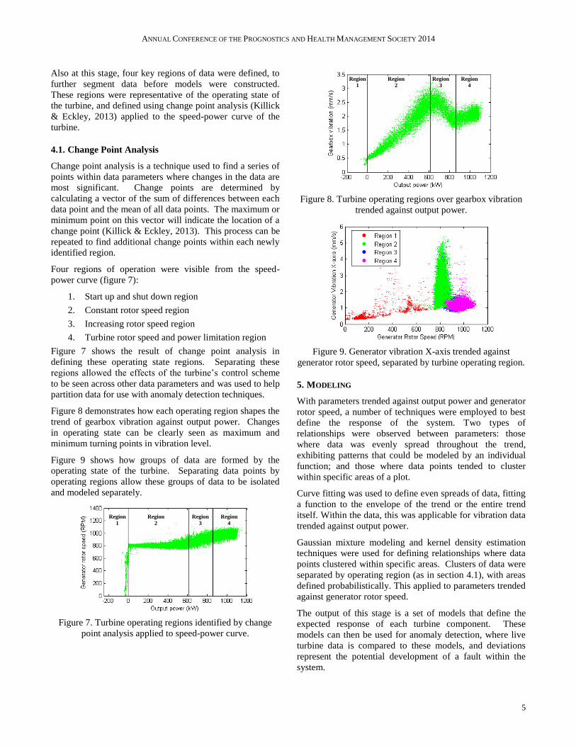
Figure 8 demonstrates how each operating region shapes the

trend of gearbox vibration against output power. Changes

in operating state can be clearly seen as maximum and

minimum turning points in vibration level.

Figure 9 shows how groups of data are formed by the

operating state of the turbine. Separating data points by

operating regions allow these groups of data to be isolated

and modeled separately.

Figure 7. Turbine operating regions identified by change

point analysis applied to speed-power curve.

Figure 8. Turbine operating regions over gearbox vibration

trended against output power.

Figure 9. Generator vibration X-axis trended against

generator rotor speed, separated by turbine operating region.

5. MODELING

With parameters trended against output power and generator

rotor speed, a number of techniques were employed to best

define the response of the system. Two types of

relationships were observed between parameters: those

where data was evenly spread throughout the trend,

exhibiting patterns that could be modeled by an individual

function; and those where data points tended to cluster

within specific areas of a plot.

Curve fitting was used to define even spreads of data, fitting

a function to the envelope of the trend or the entire trend

itself. Within the data, this was applicable for vibration data


Gaussian mixture modeling and kernel density estimation

techniques were used for defining relationships where data

points clustered within specific areas. Clusters of data were

separated by operating region (as in section 4.1), with areas

defined probabilistically. This applied to parameters trended

against generator rotor speed.

The output of this stage is a set of models that define the

expected response of each turbine component. These

models can then be used for anomaly detection, where live

turbine data is compared to these models, and deviations

represent the potential development of a fault within the

system.

Region

1

Region

2

Region

3

Region

4

Region

1

Region

2

Region

3

Region

4


6

5.1. Curve Fitting

Curve fitting was applied to data parameters trended against

output power, where relationships displayed an even spread

of data across the trend. Initially, this technique was applied

to the envelope of these trends, as maximum levels of

vibration varied with output power. Anomalies would be

detected in this case by data points exceeding maximum

expected levels of vibration, lying about a curve fitted to the

envelope.

Curve fitting was also applied to describe the trend between

gearbox vibration and output power as a whole. This would

enable additional metrics, such as variance, to be measured,

with anomalies detected where data points exceeded a

threshold of distance from the fitted curve.

Within this study, curve fitting was implemented in

MATLAB using the ‘Trust-Region-Reflective Least

Squares’ algorithm. This is an iterative method that tunes

parameters of the chosen function to

minimize the squared error between each data point

and the function itself, equation (1) (Hung, 2012).

(1)

5.1.1. Envelope Fitting

Within the data from the HS1000 turbine, parameters

trended against output power displayed varying levels of

maximum vibration across their envelopes. Curves fitted to

these envelopes will therefore describe a threshold of

maximum expected vibration levels over the full range of

turbine operation for each parameter, with anomalies

detected above this threshold.

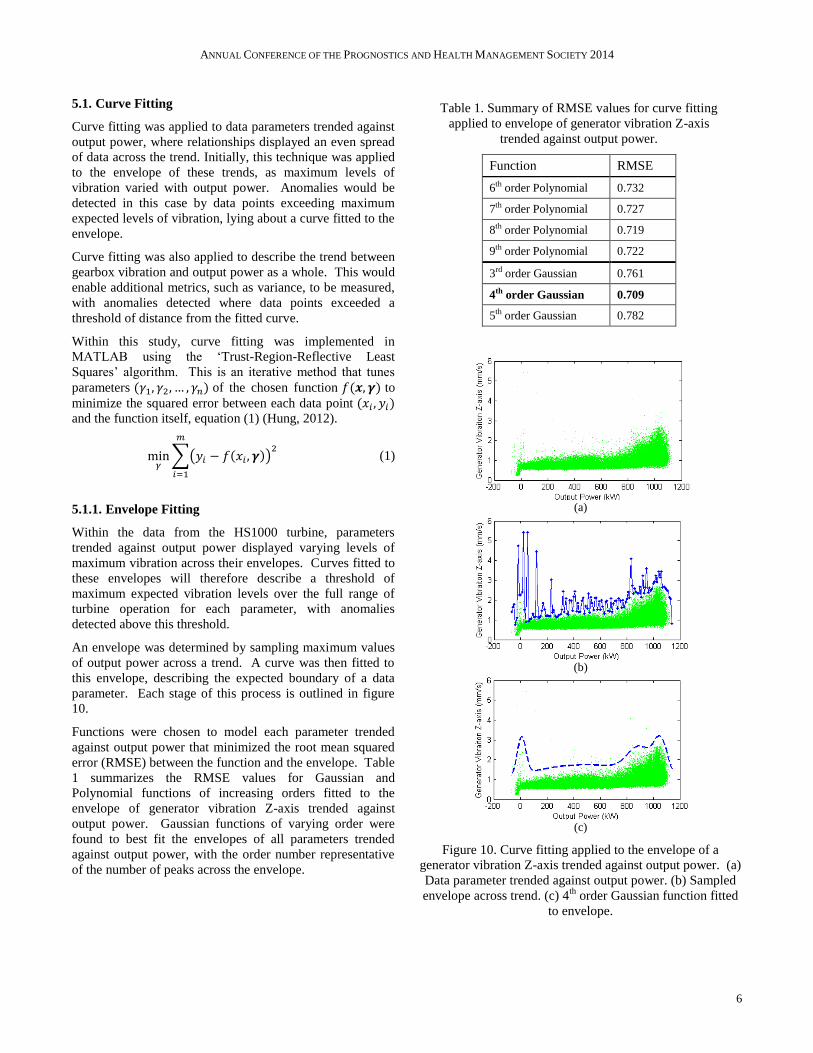
An envelope was determined by sampling maximum values

of output power across a trend. A curve was then fitted to

this envelope, describing the expected boundary of a data

parameter. Each stage of this process is outlined in figure

10.

Functions were chosen to model each parameter trended

against output power that minimized the root mean squared

error (RMSE) between the function and the envelope. Table

1 summarizes the RMSE values for Gaussian and

Polynomial functions of increasing orders fitted to the

envelope of generator vibration Z-axis trended against

output power. Gaussian functions of varying order were

found to best fit the envelopes of all parameters trended

against output power, with the order number representative

of the number of peaks across the envelope.

(a)

(b)

(c)

Figure 10. Curve fitting applied to the envelope of a

generator vibration Z-axis trended against output power. (a)

Data parameter trended against output power. (b) Sampled

envelope across trend. (c) 4th

order Gaussian function fitted

to envelope.

Table 1. Summary of RMSE values for curve fitting

applied to envelope of generator vibration Z-axis


Function RMSE

6th order Polynomial 0.732




3rd order Gaussian 0.761

4th order Gaussian 0.709

5th order Gaussian 0.782


7

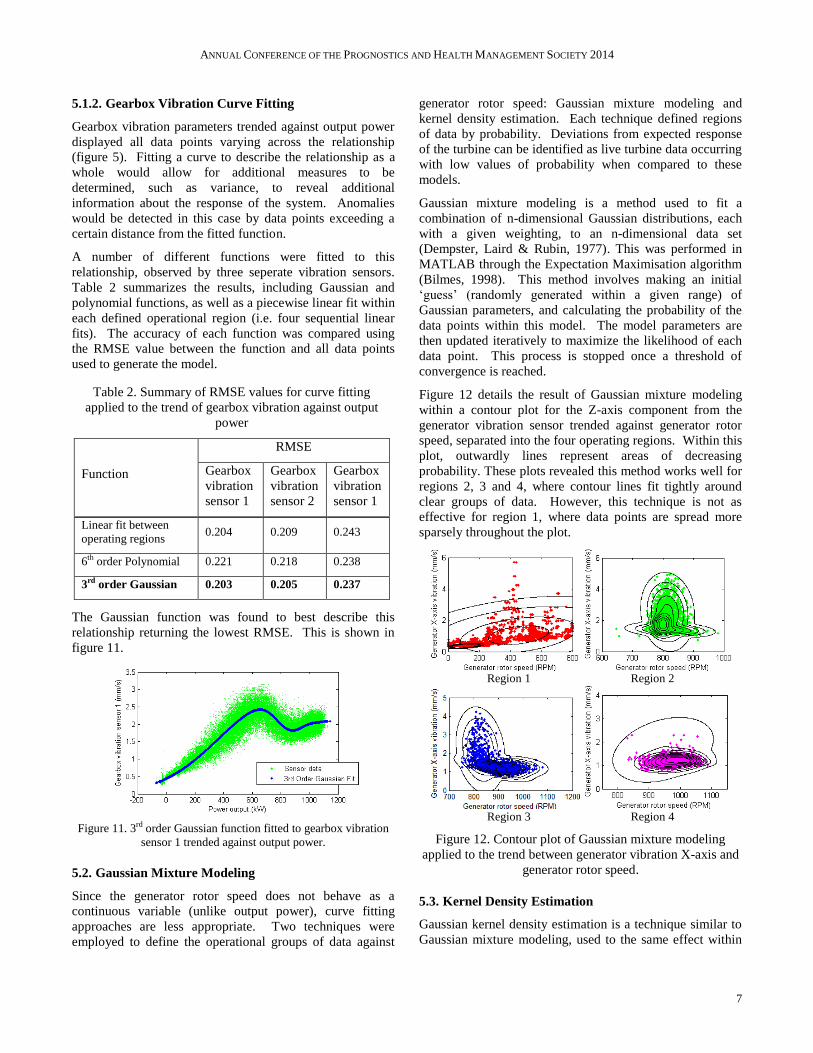
5.1.2. Gearbox Vibration Curve Fitting

Gearbox vibration parameters trended against output power

displayed all data points varying across the relationship

(figure 5). Fitting a curve to describe the relationship as a

whole would allow for additional measures to be

determined, such as variance, to reveal additional

information about the response of the system. Anomalies

would be detected in this case by data points exceeding a

certain distance from the fitted function.

A number of different functions were fitted to this

relationship, observed by three seperate vibration sensors.

Table 2 summarizes the results, including Gaussian and

polynomial functions, as well as a piecewise linear fit within

each defined operational region (i.e. four sequential linear

fits). The accuracy of each function was compared using

the RMSE value between the function and all data points

used to generate the model.

The Gaussian function was found to best describe this

relationship returning the lowest RMSE. This is shown in

figure 11.

Figure 11. 3rd order Gaussian function fitted to gearbox vibration

sensor 1 trended against output power.

5.2. Gaussian Mixture Modeling

Since the generator rotor speed does not behave as a

continuous variable (unlike output power), curve fitting

approaches are less appropriate. Two techniques were

employed to define the operational groups of data against

generator rotor speed: Gaussian mixture modeling and

kernel density estimation. Each technique defined regions

of data by probability. Deviations from expected response

of the turbine can be identified as live turbine data occurring

with low values of probability when compared to these

models.

Gaussian mixture modeling is a method used to fit a

combination of n-dimensional Gaussian distributions, each

with a given weighting, to an n-dimensional data set

(Dempster, Laird & Rubin, 1977). This was performed in

MATLAB through the Expectation Maximisation algorithm

(Bilmes, 1998). This method involves making an initial

‘guess’ (randomly generated within a given range) of

Gaussian parameters, and calculating the probability of the

data points within this model. The model parameters are

then updated iteratively to maximize the likelihood of each

data point. This process is stopped once a threshold of

convergence is reached.

Figure 12 details the result of Gaussian mixture modeling

within a contour plot for the Z-axis component from the

generator vibration sensor trended against generator rotor

speed, separated into the four operating regions. Within this

plot, outwardly lines represent areas of decreasing

probability. These plots revealed this method works well for

regions 2, 3 and 4, where contour lines fit tightly around

clear groups of data. However, this technique is not as

effective for region 1, where data points are spread more

sparsely throughout the plot.

Region 1 Region 2

Region 3 Region 4

Figure 12. Contour plot of Gaussian mixture modeling

applied to the trend between generator vibration X-axis and

generator rotor speed.

5.3. Kernel Density Estimation

Gaussian kernel density estimation is a technique similar to

Gaussian mixture modeling, used to the same effect within

Table 2. Summary of RMSE values for curve fitting

applied to the trend of gearbox vibration against output

power

Function

RMSE

Gearbox

vibration

sensor 1

Gearbox

vibration

sensor 2

Gearbox

vibration

sensor 1

Linear fit between

operating regions 0.204 0.209 0.243

6th order Polynomial 0.221 0.218 0.238

3rd order Gaussian 0.203 0.205 0.237


8

this study to define regions of probability between

parameters. However, this technique differs as it aims to

approximate the true probability density function (PDF) of

the data.

The true distribution is estimated by computing the sum of

small individual PDFs at each observed data point (Zucchi,

2003). In this case, the Gaussian distribution was used as

the individual (kernel) PDF. This method will generate a

more accurate model, however it is a lot more

computationally intensive. This was implemented in

MATLAB by adapting a method by Cao (2013).

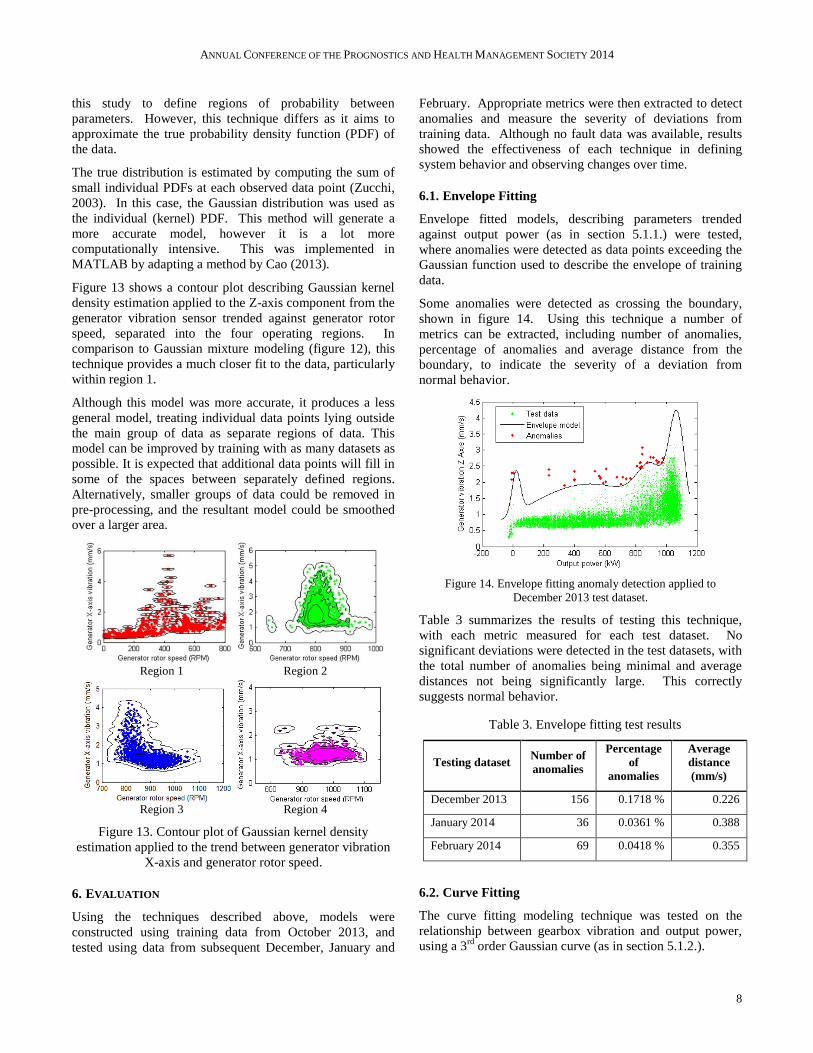
Figure 13 shows a contour plot describing Gaussian kernel

density estimation applied to the Z-axis component from the

generator vibration sensor trended against generator rotor

speed, separated into the four operating regions. In

comparison to Gaussian mixture modeling (figure 12), this

technique provides a much closer fit to the data, particularly

within region 1.

Although this model was more accurate, it produces a less

general model, treating individual data points lying outside

the main group of data as separate regions of data. This

model can be improved by training with as many datasets as

possible. It is expected that additional data points will fill in

some of the spaces between separately defined regions.

Alternatively, smaller groups of data could be removed in

pre-processing, and the resultant model could be smoothed

over a larger area.

Region 1 Region 2

Region 3 Region 4

Figure 13. Contour plot of Gaussian kernel density

estimation applied to the trend between generator vibration

X-axis and generator rotor speed.

6. EVALUATION

Using the techniques described above, models were

constructed using training data from October 2013, and

tested using data from subsequent December, January and

February. Appropriate metrics were then extracted to detect

anomalies and measure the severity of deviations from

training data. Although no fault data was available, results

showed the effectiveness of each technique in defining

system behavior and observing changes over time.

6.1. Envelope Fitting

Envelope fitted models, describing parameters trended

against output power (as in section 5.1.1.) were tested,

where anomalies were detected as data points exceeding the

Gaussian function used to describe the envelope of training

data.

Some anomalies were detected as crossing the boundary,

shown in figure 14. Using this technique a number of

metrics can be extracted, including number of anomalies,

percentage of anomalies and average distance from the

boundary, to indicate the severity of a deviation from

normal behavior.

Figure 14. Envelope fitting anomaly detection applied to

December 2013 test dataset.

Table 3 summarizes the results of testing this technique,

with each metric measured for each test dataset. No

significant deviations were detected in the test datasets, with

the total number of anomalies being minimal and average

distances not being significantly large. This correctly

suggests normal behavior.

6.2. Curve Fitting

The curve fitting modeling technique was tested on the

relationship between gearbox vibration and output power,

using a 3rd

order Gaussian curve (as in section 5.1.2.).

Table 3. Envelope fitting test results

Testing dataset Number of

anomalies

Percentage

of

anomalies

Average

distance

(mm/s)

December 2013 156 0.1718 % 0.226

January 2014 36 0.0361 % 0.388

February 2014 69 0.0418 % 0.355


9

Figure 15 shows the December 2013 testing data compared

against a trained model constructed from October 2013 data.

In contrast to envelope model fitting, no set boundary is

used to indicate anomalous data points. Instead, metrics

such as maximum error and RMSE can be used to measure

the severity of any deviation from normal system response.

Figure 15. Curve fitting anomaly detection applied to December

2013 test data.

Table 4 summarizes testing results using these metrics. An

increase in RMSE is seen in both December and February

where more data points are lying above the Gaussian

function, indicating an overall increase in vibration across

the full operating range. This was attributed to seasonal

changes in tidal flow affecting the test data, and not

component wear or damage.

6.3. Gaussian Mixture Modeling

Gaussian mixture modeling was tested on clusters of

generator vibration data trended against generator rotor

speed, separated by operational regions, as described in

sections 4.1. and 5.2. Results detailed in this section were

recorded from the generator X-axis vibration parameter.

Anomalies were considered to be data points lying outside

the 95% confidence interval. The percentage of anomalies

lying outside the 95% confidence interval (CI) was used as a

metric. A value exceeding 5% was considered to indicate

that the model was not a good fit to the test data and a

change in system response may have occurred.

Table 5 and figure 16 show the results of testing. A number

of clusters were identified to have a significant number of

anomalies, with percentages exceeding 5%. These results

indicate a deviation in system response over time, however,

the variations were due to seasonal changes in tidal flow.

The significant number of anomalies is therefore not

representative of the relatively small variation in data, and it

was concluded that Gaussian mixture modeling provided a

poor representation of training data distributions.

Region 1 Region 2

Region 3 Region 4

Figure 16. Gaussian mixture modeling anomaly detection applied

to December 2013 test data.

Table 5. Gaussian mixture modeling test results

Testing dataset Region

No. of

Anomalies

outside 95% CI

Percentage

of

anomalies

December 2013

1 59 1.006

2 1532 4.454

3 1425 9.799

4 7180 19.928

January 2014

1 88 0.821

2 347 1.998

3 194 1.552

4 10350 19.938

February 2014

1 2469 5.776

2 6031 5.519

3 1986 15.055

4 19 52.777

Table 4. Curve fitting test results

Training dataset Max Error

(mm/s)

RMSE

(mm/s)

October 2013 1.45 0.203

Testing dataset Max Error

(mm/s)

RMSE

(mm/s)

December 2013 1.26 0.251

January 2014 0.93 0.202

February 2014 1.04 0.235


10

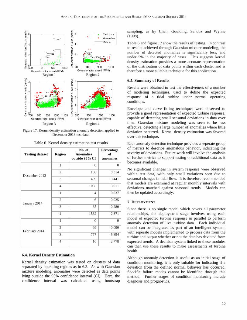
Region 1 Region 2

Region 3 Region 4

Figure 17. Kernel density estimation anomaly detection applied to

December 2013 test data.

6.4. Kernel Density Estimation

Kernel density estimation was tested on clusters of data

separated by operating regions as in 6.3. As with Gaussian

mixture modeling, anomalies were detected as data points

lying outside the 95% confidence interval (CI). Here, the

confidence interval was calculated using bootstrap

sampling, as by Chen, Goulding, Sandoz and Wynne

(1998).

Table 6 and figure 17 show the results of testing. In contrast

to results achieved through Gaussian mixture modeling, the

number of detected anomalies is significantly less, and

under 5% in the majority of cases. This suggests kernel

density estimation provides a more accurate representation

of the distribution of data points within each cluster and is

therefore a more suitable technique for this application.

6.5. Summary of Results

Results were obtained to test the effectiveness of a number

of modeling techniques, used to define the expected

response of a tidal turbine under normal operating

conditions.

Envelope and curve fitting techniques were observed to

provide a good representation of expected turbine response,

capable of detecting small seasonal deviations in data over

time. Gaussian mixture modeling was seen to be less

effective, detecting a large number of anomalies where little

deviation occurred. Kernel density estimation was favored

over this technique.

Each anomaly detection technique provides a seperate group

of metrics to describe anomalous behavior, indicating the

severity of deviations. Future work will involve the analysis

of further metrics to support testing on additional data as it

becomes available.

No significant changes in system response were observed

within test data, with only small variations seen due to

seasonal changes in tidal flow. It is therefore recommended

that models are examined at regular monthly intervals with

deviations matched against seasonal trends. Models can

then be updated accordingly.

7. DEPLOYMENT

Since there is no single model which covers all parameter

relationships, the deployment stage involves using each

model of expected turbine response in parallel to perform

anomaly detection of live turbine data. Each individual

model can be integrated as part of an intelligent system,

with seperate models implemented to process data from the

turbine and output whether or not the data has deviated from

expected trends. A decision system linked to these modules

can then use these results to make assessments of turbine

health.

Although anomaly detection is useful as an initial stage of

condition monitoring, it is only suitable for indicating if a

deviation from the defined normal behavior has occurred.

Specific failure modes cannot be identified through this

method. Further stages of condition monitoring include

diagnosis and prognostics.

Table 6. Kernel density estimation test results

Testing dataset Region

No. of

Anomalies

outside 95% CI

Percentage

of

anomalies

December 2013

1 0 0

2 108 0.314

3 499 3.441

4 1085 3.011

January 2014

1 4 0.037

2 6 0.025

3 35 0.280

4 1532 2.871

February 2014

1 0 0

2 99 0.090

3 777 5.894

4 10 2.778


11

Diagnosis involves analysis of turbine component failure

modes, and understanding how these will be represented

within data parameters. Prognostics involve assessing the

current state of the system and estimating the remaining

useful life of individual components, or the system as a

whole. Various algorithms can be used for these purposes,

including those used within machine learning and artificial

intelligence, such as neural networks or Bayesian classifiers.

Future work will explore these algorithms in relation to the

system, utilizing failure data as it becomes available.

Diagnostics and prognostics can be implemented as

additional modules in the intelligent system.

8. CONCLUSION

This paper outlined the use of data mining through the

CRISP-DM process model to explore data from the HS1000

tidal turbine and define its expected operational behavior.

The use of principal component analysis and correlation

revealed key relationships within the data, relating

parameters to output power and generator rotor speed.

Envelope and curve fitting techniques were found to provide

accurate models of the response of system components to

changes in output power. Kernel density estimation was

also found to be an effective technique when used to model

clusters of generator vibration data formed when trended

against rotor speed. Gaussian mixture modeling was found

to be less effective in this application.

Models were trained using past operational turbine sensor

data, with anomaly detection performed using data from

subsequent months. Small deviations in system response

were detected, due to seasonal changes in tidal flow.

Future work will involve the analysis of further metrics to

describe the severity of anomalous responses, using

additional data as it becomes available. Once techniques are

established, an intelligent condition monitoring system will

be designed to integrate seperate modules together and

assess the state of the turbine and its components. With

further research, additional modules can be added to the

intelligent system, to perform diagnosis and prognosis as

failure data becomes available.

9. REFERENCES

Abdi, H. & Williams, L. (2010). Principle Component

Analysis. Wiley Interdisciplinary Reviews:

Computational Statistics, 2(4), pp. 433-459

Aly, H. H. H., El-Hawary, M. E. (2011). State of the Art for

Tidal Currents Electric Energy Resources. 24th

Canadian Conference on Electrical and Computer

Engineering (CCECE) (1119-1124), May 8-11, Niagra

Falls, ON. doi:10.1109/CCECE.2011.6030636

Bilmes, J. (1998). A Gentle Tutorial of the EM algorithm

and its Application to Parameter Estimation for

Gaussian Mixture and Hidden Markov Models.

Technical Report ICSI-TR-97-021, University of

Berkeley

Cao. Y. (2013). Bivariant Kernel Density Estimation (V2.1).

http://www.mathworks.co.uk/matlabcentral/fileexchang

e/19280-bivariant-kernel-density-estimation-v2-

1/content/html/gkde2test.html

Chen, H., Ait-Ahmed, N., Zaim, E. & Machmoum, M.

(2012). Marine Tidal Current Systems: state of the art.

2012 IEEE International Symposium on Industrial

Electronics (1431-1437), May 28-31, Hangzhou, China.

doi:10.1109/ISIE.2012.6237301

Chen, Q., Goulding, P., Sandoz, D. & Wynne R. (1998).

The Application of Kernel Density Estimates to

Condition Monitoring for Process Industries.

Proceedings of the American Control Conference (pp

3312-3316). June 1998, Philadelphia, PA. doi:

10.1109/ACC.1998.703187

Dempster, A. P., Laird, N. M. & Rubin, D. B. (1997).

Maximum-likelihood from incomplete data via the EM

algorithm. Journal of the Royal Statistical Society,

Series B, 39(1), pp. 1-38. doi: 10.1.1.133.4884

Duhaney, J., Khoshgoftaar, T. M., Sloan, J. C., Alhalabi, B.

& Beaujean, B. (2011). A Dynamometer for an Ocean

Turbine Prototype – Reliability through Automated

Monitoring. 2011 IEEE 13th International Symposium

on High-Assurance Systems in Engineering (pp 244-

251). November 10-12, Boca Raton, FL. doi:

10.1109/HASE.2011.61

European Union Committee (2008). The EU’s Target for

Renewable Energy: 20% by 2020, 27th

Report of

Session 2007-08

Hung, J. (2012). Energy Optimization of a Diatomic System.

University of Washington, Seattle, WA.

http://www.math.washington.edu/~morrow/papers/jane

-thesis.pdf

Killick, R. & Eckley, I. A. (2013). Changepoint: An R

Package for Changepoint Analysis. Lancaster

University, UK.

King, J. & Tryfonas, T. (2009). Tidal Stream Power

Technology – State of the Art. OCEANS 2009 –

EUROPE (1-8). May 11-14, Bremen.

doi:10.1109/OCEANSE.2009.5278329

Mahfuz, H. & Akram, M. W. (2011). Life Prediction of

Composite Turbine Blades under Random Ocean

Current and Velocity Shear. OCEANS 2011 IEEE –

SPAIN (1-7). June 6-9, Santander. doi:10.1109/Oceans-

Spain.2011.6003526

Maimon, O., Rokach, L. (2005). Data Mining and

Knowledge Discovery Handbook. New York, NY:

Springer

Olson, D. L., Delen, D. (2008). Advanced Data Mining

Techniques. Heidelberg: Springer

Pearson, K. (1901). On Lines and Planes of Closest Fit to

Systems of Points in Space. Philosophical Magazine,

2(11), pp. 559-572


12

Prickett, P., Grosvenor, R., Byrne, C., Jones, A. M., Morris,

C., O’Doherty, D. & O’Doherty, T. (2011).

Consideration of the Condition Based Maintenance of

Marine Tidal Turbines. 9th

European Wave and Tidal

Energy Conference. September 5-9, Southampton UK.

Rodgers, J. L. & Nicewander, W. A. (1988). Thirteen Ways

to Look at the Correlation Coefficient. The American

Statistician, 42(1), pp. 59-66

Wald, R., Khoshgoftaar, T. M., Beaujean, B. & Sloan, J. C.

(2010). A Review of Prognostics and Health

Monitoring Techniques for Autonomous Ocean

Systems. 16th

ISSAT International Conference

Reliability and Quality in Design. August 5-7,

Washington, D.C.

Winter, A. I. (2011). Differences in Fundamental Design

Drivers for Wind and Tidal Turbines. OCEANS, 2011

IEEE – SPAIN (1-10), June 6-9, Santander. doi:

10.1109/Oceans-Spain.2011.6003647

Wirth, R. & Hipp, J. (2000). CRISP-DM: Towards a

standard process model for data mining. Proceedings of

the Fourth International Conference on the Practical

Application of Knowledge Discovery and Data Mining

(29-39), Manchester, UK.

Zucchi, W. (2003). Applied Smoothing Techniques, Part 1:

Kernel Density Estimation. Philadelphia, Pa: Temple

University

BIOGRAPHIES

Grant S. Galloway is a PhD student within the Institute for

Energy and Environment at the University of Strathclyde,

Scotland, UK. He received his M.Eng in Electronic and

Electrical Engineering from the University of Strathclyde in

2013. His PhD focuses on condition monitoring and

prognostics for tidal turbines, in collaboration with Andritz

Hydro Hammerfest, a leading tidal turbine manufacturer.

Victoria M. Catterson is a Lecturer within the Institute for

Energy and Environment at the University of Strathclyde,

Scotland, UK. She received her B.Eng. (Hons) and Ph.D.

degrees from the University of Strathclyde in 2003 and 2007

respectively. Her research interests include condition

monitoring, diagnostics, and prognostics for power

engineering applications.

Craig Love is a Turbine System Engineer with Andritz

Hydro Hammerfest, Glasgow, UK.

Andrew Robb is a Mechanical Engineer with Andritz

Hydro Hammerfest, Glasgow, UK.

anomaly detection techniques for the condition monitoring ... · anomaly detection techniques for...

Documents