MARINE ECOLOGY PROGRESS SERIESMar Ecol Prog Ser

Vol. 449: 245–262, 2012doi: 10.3354/meps09528

Published March 8

INTRODUCTION

The ocean environment and the prey field encoun-tered by migrating salmon is far from static; it is com-plex, dynamic and in flux over multiple spatial andtemporal scales (Mackas et al. 2004, 2007). Thereforethe fate of salmon may depend on where and howlong they reside in particular areas of the Pacific. The

first few weeks to months following ocean entry arethought to be a critical time for survival, as fish mustgrow fast and large and accumulate sufficient energyreserves to escape both predation-based and starva-tion-based mortality as these are size-dependent(Willette et al. 2001, Hurst 2007, Trudel et al. 2007,MacFarlane 2010, Duffy & Beauchamp 2011). It isnow widely accepted that salmon growth rates are

© Fisheries and Oceans Canada 2012Publisher: Inter-Research · www.int-res.com

*Email: strahan.tucker@dfo-mpo.gc.ca

Annual coastal migration of juvenile Chinooksalmon: static stock-specific patterns in a highly

dynamic ocean

S. Tucker1,*, M. Trudel1,2, D. W. Welch1,3, J. R. Candy1, J. F. T. Morris1, M. E. Thiess1, C. Wallace1, T. D. Beacham1

1Pacific Biological Station, Fisheries and Oceans Canada, 3190 Hammond Bay Rd, Nanaimo, British Columbia V9T 6N7, Canada2Department of Biology, University of Victoria, Victoria, British Columbia V8W 3N5, Canada

3Present address: Kintama Research Services Ltd, 10-1850 Northfield Road, Nanaimo, British Columbia V9S 3B3, Canada

ABSTRACT: While recent studies have evaluated the stock-specific coastal migration of juvenileChinook salmon, it remains unclear if these seasonal patterns are consistent between years, partic-ularly when ocean conditions change dramatically. Here we contrast the abundance, distributionand seasonal stock compositions of juvenile Chinook salmon between years in 3 oceanographic re-gions of the Pacific from southern British Columbia to southeast Alaska. Between 1998 and 2008,we surveyed salmon in various months from June through March, in different regions along theshelf. Variable conditions in the North Pacific Ocean, as well as large overall shifts in ocean regimeswere extensively documented over this decade. We employed genetic stock identification toidentify mixed-stock compositions; fish (n = 6274) were allocated to one of 15 regional and 40 sub-regional stocks. Catch-per-unit-effort and distribution of salmon, as denoted by centre of mass, var-ied significantly between seasons, regions and years. In a similar manner, fish body size and dry-weight varied significantly between years, seasons and regions. Despite these inter-annualdifferences in catch, distribution, fish growth performance and large variations in ocean conditionsencountered by salmon over the time period of the study, we observed no response in terms of shiftsin stock-specific distributions. Regional stock composition was similar between years, suggestingmigration patterns for all stocks remain consistent despite fluctuations in the marine environment:local stocks remain resident in respective coastal areas during their first year at sea, except for Columbia River salmon, which move quickly into waters north of Vancouver Island in summer.

KEY WORDS: Juvenile Chinook salmon · Ocean migration · DNA stock identification · Variable ocean conditions

Resale or republication not permitted without written consent of the publisher

OPENPEN ACCESSCCESS

Mar Ecol Prog Ser 449: 245–262, 2012

coupled to ocean conditions (Pearcy 1992, Mueter etal. 2002, Quinn et al. 2005). However, direct mecha-nisms linking ocean conditions, growth and survivalare elusive and likely complex (Trudel et al. 2007).This is because trends in growth and marine survivalamong different stocks, even for geographicallyadjacent stocks, are not always consistent and areoften asynchronous, suggesting there are potentialdifferences in migration or ocean residency patterns(Hare et al. 1999, Mueter et al. 2002, Wells et al.2008). Clearly, an important component is establish-ing where juvenile salmon live during their first fewmonths in the ocean. Then we can explore not onlythe physical and biological variables that mightaffect salmon growth and survival but also whethersalmon respond to changes in ocean conditions byaltering their movement patterns.

Chinook salmon Oncorhynchus tshawytscha arewidely distributed along the west coast of NorthAmerica, ranging from central California to northernAlaska (Healey 1991). Chinook salmon go to seaeither within a few months of hatching (sub-yearlingsmolts), or following a full year in fresh water (year-ling smolts). Yearling type smolts predominate in theNorth (north of 56°N), whereas sub-yearling smoltsare almost exclusively distributed in the South(Healey 1991). The main exceptions are the Fraserand the Columbia River systems, as well as popula-tions in northern Puget Sound where both types arefound (Healey 1991, Teel et al. 2000, Waples et al.2004).

Recent studies have focused both on definingmarine habitat use for juvenile Chinook salmon (Biet al. 2007, 2008, 2011a, Peterson et al. 2010) andthe relationship between variable ocean conditionsand abundance, growth or condition (Wells et al.2008, MacFarlane 2010). The presence and abun-dance of Chinook salmon is negatively correlatedwith water temperature and depth, and positivelycorrelated to various production indices such aschlorophyll (chl) a concentration and zooplankton(copepod) biomass (Brodeur et al. 2000, 2004, Fisheret al. 2007, Bi et al. 2007, 2011a, Peterson et al.2010). These correlations between juvenile salmonabundance and environmental variables are gener-ally weak and shift seasonally (Brodeur et al. 2004).Not all of these studies examined inter-annual dif-ferences in distribution explicitly: some wereregionally restricted, and all have dealt with aggre-gate samples of salmon; generally only one smolt-type is considered and these fish are likely a mix-ture of different stocks (Trudel et al. 2009, Tucker etal. 2011). Given that Chinook salmon are associated

with particular environmental conditions, thoughnot specific ones (i.e. always found within a range,which changes seasonally) it seems plausible thatsalmon would adjust their migration patterns basedon conditions encountered once at sea. Indeed, Chi-nook salmon abundance and distribution along thecoasts of Washington and Oregon is patchy andhighly variable between cold and warm ocean years(Bi et al. 2008, Peterson et al. 2010). However with-out geographically widespread, concurrent sam-pling across the coastal shelf, coupled with knowl-edge of the origin of these fish, it remains unclear ifvariation in abundance trends for juveniles is afunction of dispersal or survival.

While much research has been directed at studyingthe ecology and habitats occupied by juvenile sal -mon in the sea (reviewed by Brodeur et al. 2000,Pearcy 1992), our understanding of the stock-specificdistribution and movement patterns of juvenile sal -mon in the ocean has only increased recently (Morriset al. 2007, Murphy et al. 2009, Trudel et al. 2009,Tucker et al. 2009, 2011, Rechisky et al. 2009, Welchet al. 2009, 2011, J. Fisher unpubl.). Seasonal migra-tion patterns have been reconstructed through theanalysis of both coded-wire tag (CWT) recoveriesand the application of DNA stock identification tech-niques. These studies have underlined the impor-tance of considering relevant spatial scales forassessing the effects of ocean conditions on Pacificsalmon as migration varies with species, stock andlife history (Trudel et al. 2009, Tucker et al. 2011,J. Fisher unpubl.). For Chinook salmon, stocks arefound to remain in coastal waters near their river oforigin during their 1st yr at sea irrespective of smolttype, northward migration is not initiated until the2nd yr at sea (Trudel et al. 2009, Murphy et al. 2009,Tucker et al. 2011). The exceptions are yearlingsmolts from southern stocks (Fraser River, PugetSound, coastal Washington and Oregon, ColumbiaRiver), which move quickly into waters north of Van-couver Island, including southeast Alaska; sub-year-ling smolts from these stocks remain in waters of theCalifornia Current System and Puget Sound (Trudelet al. 2009, Duffy & Beauchamp 2011, Tucker et al.2011, J. Fisher unpubl.). What remains unclear is ifthese seasonal patterns are consistent betweenyears, particularly when ocean conditions changedramatically.

Patterns of movement are considered a key factorin the survival of most organisms (e.g. Turchin 1998,Fritz et al. 2003) as many animals must move tofeed. Therefore, we might expect migration patternsto deviate with local or regional conditions and prey

246

Tucker et al.: Annual coastal migration of Chinook salmon

availability. However, the observation of differentialgrowth and survival between northern and southernpopulations of salmon (Wells et al. 2008) suggeststhat the ability of juvenile Chinook salmon tochange their migratory behaviour in response tochanging climate and ocean conditions might belimited; either they are simply unable to move out ofregions with ‘poor’ conditions, or they are geneti-cally constrained to simply do the same thing everyyear. However, there is evidence for both plasticityand inflexibility in salmon migration behaviour. Forexample, Bea mish et al. (2002) reported dramaticchanges in the behaviour of coho salmon Onco -rhynchus kisutch in the Strait of Georgia coupled toabrupt climate changes, with virtually all (formerlyresident) coho salmon moving out of the Straitunder particular climate regimes. On the otherhand, consistent stock-specific differences wheretagged salmon are caught in the ocean have beenobserved. Both maturing coho and Chinook salmondisplay stock-specific marine distributions, whichfor the most part, are distinct from other stocks andconsistent between years despite large fluctuationsin ocean conditions (Weit kamp & Neely 2002,Weitkamp 2010). However, these fish were inter-cepted in coastal fisheries on their return to fresh-water to spawn; hence, it is not entirely certain theyresided in different parts of the ocean. Differencesin stable isotope values in maturing sockeye salmonsuggest that there may be some spatial segregationin marine distribution between stocks as well asamong sockeye populations within the Fraser Riversystem itself (Welch & Parsons 1993, Satterfield &Finney 2002).

Here we contrast the abundance, distribution andseasonal stock compositions of juvenile Chinooksalmon between years in 3 coastal shelf regions ofthe Pacific from southern British Columbia to south-east Alaska. The objective was to test for consistencyin stock-specific migration patterns over a decade(1998 to 2008) that saw large fluctuations in oceanconditions (e.g. DFO 2009). Secondarily, we alsoevaluate whether there were in fact differences inbody size (inferred growth rates) and energy densi-ties within each season and region to evaluate poten-tial annual differences in juvenile Chinook salmongrowth performance. We employ genetic stock iden-tification techniques to identify mixed-stock compo-sitions in coast-wide samples. Recently, we validatedgenetic population assignments by showing that96% of known-origin coded wire tagged Chinooksalmon were accurately allocated to their region oforigin (Tucker et al. 2011).

Oceanographic setting

Across their range, North American Chinook sal -mon encounter a number of distinctive ocean regionsin the North Pacific. These have diverse physical andchemical oceanographic attributes as well asdifferent biological communities (Batten et al. 2006,Batten & Freeland 2007, Hickey & Banas 2008). Theeastward flowing Sub-Arctic Current bifurcates as itapproaches the North American coast into the equa-tor-ward flowing California Current System (CCS)and the pole-ward flowing Alaskan Coastal Current(ACC; Wells et al. 2008). These currents are drivenby the relative strength of the Aleutian low pressurecell and North Pacific high pressure cell (Strub &James 2002). The North American Pacific coast canconsequently be divided into 3 general oceano-graphic regions: an upwelling zone south of Vancou-ver Island within the CCS, a downwelling zone northof Vancouver Island within the ACC, and a transitionzone between the two (Wells et al. 2008). In the ACC,phytoplankton productivity is generally limited bylight rather than by nutrients (Ware & McFarlane1989, Gargett 1997) while the CCS is primarily nutri-ent limited. Although total zooplankton biomass andproductivity are strongly dominated by calanoidcopepods in both systems, the mix of species varies(Mackas et al. 2004). Copepods are generally largerand richer in lipids in the ACC (Båmstedt 1986, Za-mon & Welch 2005) while temperature, phytoplank-ton and zooplankton biomass are higher in the CCS(Ware & Thomson 2005). Oceanographic differences,as well as differences in phytoplankton and zoo-plankton communities are paralleled by general dif-ferences in fish community composition and abun-dances (Orsi et al. 2007). In terms of proportions oftotal catch, the CCS is dominated by clupeids such asPacific sardines Sardinops sagax, northern anchoviesEngraulis mordax, and Pacific herring Clupea palla -si, while the ACC is dominated by juvenile salmonidswith a distinct breakpoint in species assemblages offVancouver Island (Orsi et al. 2007); frequencies of oc-currence of salmonids in catches are however almostequally as high in both regions. This study encom-passed the northern portion of the CCS off the westcoast of Vancouver Island, and the southern portionof the ACC off southeast Alaska as well as the transi-tion zone in between the 2 current systems.

Despite the recognizable oceanographic regions,these areas are not static and demonstrate bothstrong seasonality as well as variability in response tomultiple factors including coastal winds, freshwaterrunoff, solar heating, light conditions, atmospheric

247

Mar Ecol Prog Ser 449: 245–262, 2012

pressure, and offshore oceanic conditions (Wells et al.2008). The seasonal cycles in turn, are modified andthe variability is closely coupled with large scaleevents and conditions throughout the tropical andsub-arctic North Pacific Ocean, including frequent ElNiño and La Niña events (particularly over the pastdecade). Large-scale variation in climate driveslarge-scale changes in ocean temperatures (Mantuaet al. 1997) with attendant ecosystem effects. Some ofthe largest ‘regime’ shifts in the North Pacific of therecent past include rapid warming in the mid 1970s,cooling in the mid-late 1980s, warming from the early1990s through 1998, rapid cooling in 1999 with con-tinued negative temperature anomalies until 2002,and renewed warming from 2003 until 2007 (DFO2009). In 2008, waters off the Pacific coast of BritishColumbia and the Southern US coast abruptlychanged to the coldest observed in 50 yr, with thecooling extended far into the Pacific Ocean and cor-responding large-scale changes in the plankton com-munity (DFO 2009). The strength of the 2 main north-east Pacific current systems varies among yearsdepending on the intensity of the Aleutian Low pressure system (Hollowed & Wooster 1992) and arenegatively correlated both intra- and inter-annually(Ware & McFarlane 1989). Changes in horizontaltransport and water temperatures due to regimeshifts generally result in north−south shifts in the zoo-plankton community composition and the relativeabundance of large and lipid-rich northern copepods(Mackas et al. 2004, Zamon & Welch 2005, Peterson2009, Bi et al. 2011b) as well as shifts in fish commu-nity composition (Orsi et al. 2007). This affects lipid

dynamics at the base of the food web. Prey quality, interms of the lipid quantity of food, is thought to be animportant determinant in growth rates of salmon(Trudel et al. 2007, MacFarlane 2010). Recent investi-gations of alongshore transport suggests strong link-ages among climate conditions (state of the Pa cificDecadal Oscillation), direction of transport, zooplank-ton biomass and marine survival of juvenile cohosalmon in the CCS (Bi et al. 2011b). Competition forfood is expected to be more intense in the presence ofhigh numbers of clupeids given that juvenile salmonfeed on similar prey (Beamish et al. 2001, Trudel et al.2007, Orsi et al. 2007). It follows that productivity andsurvival of salmon originating from different regionswould be negatively correlated (Hare et al. 1999,Mueter et al. 2002). However, Chinook salmongrowth rates from across these regions are not corre-lated (Wells et al. 2006), probably because the migra-tory behavior of Chinook salmon often places fishfrom one region into another (Healey 1991, Trudel etal. 2009, Tucker et al. 2011, J. Fisher unpubl.).

MATERIALS AND METHODS

Sample collection

Our surveys involve both repeated cross-shelf tran-sects and opportunistic sampling from southernBritish Columbia to southeast Alaska between 1998and 2008 (Fig. 1, Table 1). The sampling surveyswere conducted in various months from Junethrough March, thus allowing reconstruction of sea-

248

SEAK

WCVI

CC

Jun–Juln = 689

SEAK

WCVI

CC

Oct–Novn = 1260

SEAK

WCVI

CC

Feb–Marn = 759

++++++++++++ ++++ +++++++ ++++++ +++ ++++++++ + +++ +++ ++++ +++ ++ +++++++++ ++ +++++ ++++++++++++++ ++++++++++ +++++++++++++++++++++++++++++++++++++++++++++++++++++++++++++++++++++++++++++

++++++++

++++++++

+

++++++++++++

+++++++++++++++++++++++++

+++++++++++++++++++++++++++++++++++++++++++++++++++++++++++++++++++++++++++++++++++++++++++++++++++++++++ +

+++++++++++++++++ +++++++++++++++++++++++++++++++++++++++++++ +++++++++++++ +++++

+++++++++++++++++++ +++ ++++ +++ ++ ++++++++ +++++++ ++++ ++++++ ++++ ++++++++++++++++++++++++++++++++++++++++++++++++++++++++++++++++++++++++++++++++++++++ ++++++ ++ +++ ++++ ++++ ++ +++ +++++ +++ ++++++++++++ ++++++++++++ ++++++++ +++ +++ ++++ ++ ++++ ++++

+++ +++ ++ ++ +++++ +++++ ++++++++ +++ +++++++++++++++ ++++++++++++ ++++++++++++++++++++++++++++++++++++++++++++++++++++++++++++++++++++++++++

++++++++++++++++++++++++++++++++++++++++++++++++++++ ++ ++ + ++ ++ ++++ +++ ++++++++++++++ ++++++++++++++++++++++++++ +++++++++++++ ++ ++ ++++ +++++++++++++ +++++++++++++++++++++++++++++++++++++++++++++++++++++++

+++++ ++++++++++++ ++++++++ +++++++ +++++ ++++ +++++ ++++ ++++++++ +++++++ +++++++ ++ ++++++ ++ +++++++ +++++ +++++++++++++ ++++ ++++++++++++++++++++ +++++++ ++ +++++++ +++++++ ++++++++ ++ +++++++ ++++ ++++ +++ +++ +++ ++++ +++ ++ +++++ ++ ++ ++++++ ++ +++++++++ +++ ++++++++++ ++++++ +++++++++ ++++++++++++ +++ +++++++++++++++++

+++++++++++++++++++++++++++++++++++++++++++++++++++++++++++++++++++++++++++++++++++++++++++++++++++++++++++++++++++++++++++++++++++++++++++++++++++++++++++++++++++++++++++++++++++++++++++++++++++++++++++++++++

++++++++

+++ +++++++++++++++++++++++++++++++++++++++++++++++++++ ++++++++++++++

+++++++++++++++++++++++++++++++++++++++++ ++++++++++++++++++ +++ ++++++++++++++ ++++++++++++++++++++++++++++++++++++++++++++++ +++ +++ ++++++ ++++ ++++ ++ ++ ++ ++

+++++ ++++++ ++++ +++ ++++++ +++++++++++ +++++ ++ ++ ++++++++++++++++++++++++++++++++++++++++++++++++++++++ ++++++++++++++++++++++++++++++++++++++++++++++++++++++++++++++ ++ +++ ++++++++ ++++ +++ ++ ++ +++++ ++++++++++ +++ ++++++ +++ +++++

++++ ++++++++ +++ +++ +++++++++++++++++++++++++ ++++++++++++++++ ++ ++++ ++++ ++++++++++++++++++ ++++++++++

++++++++++++++++++++++++++++

+ ++ +++ ++ ++ ++++ ++ +++ +++++++++++++++++++++++++++++++++++++++++

+++++ ++ + ++ +++ ++ +++ ++++++ +++++ ++++++++ +++ ++++++ +++++++++++++++++++ +++ ++++++ ++++++++ ++++ ++++++++ + +++ ++ +++ +++ +++ ++++++ +++ +++ +++++++++++++++++++++++++++ +++++

++++++++++++++++++++++++++++++++++++++++++++++++++++++++++++++++++++++++++++++++++++++++++++++++++++++++++++++++++++++++++++++++++++++++++++++++++++++++ +++++++++++++++++

++++++

+ +++++++++++++++++++++++++++++++++

+

+++++++++++ ++ ++

+++++++++++++++++++++++++++++++++++ ++++ +++

+++++++

+++++++ ++ ++ +++ +++++ ++++ ++ +++++++++ +++++++++ ++++++++++++++++++++++++++++++++++++++++++++++ ++++++++++++++++++++++++++++++ +++++ +++ ++++ +++ ++ +++++++ ++++++++++++ + ++++ ++

Fig. 1. Sampling locations in summer, fall, and spring. Crosses: individual fishing stations; sample sizes (n) report total numberof sets. Solid lines at margin of continental shelf: 200 m and 1000 m depth contours. WCVI: west coast of Vancouver Island;

CC: central British Columbia; SEAK: southeast Alaska

Tucker et al.: Annual coastal migration of Chinook salmon

sonal changes in stock composition for differentregions along the shelf (Tucker et al. 2011). A hexa -gonal mesh mid-water rope trawl (~90 m long × 30 mwide × 18 m deep, cod-end mesh 0.6 cm, CantrawlPacific) was towed at the surface (0 to 20 m) for 15 to30 min at 5 knots using primarily the CCGS‘W.E. Ricker’, or a chartered fishing vessel when itwas unavailable (i.e. ‘Ocean Selector’ June 2002;‘Frosti’ June and October 2005; ‘Viking Storm’ Octo-ber 2007, March and June 2008). Sampling was con-ducted between 06:00 and 20:00 h (Pacific Time). Amaximum of 30 Chinook salmon were randomlyselected from each net tow, and fork length and masswere determined onboard the research vessel (n =12 690). In the lab, a sub-sample (n = 5886) of fish wasdried at 60°C to constant weight to determine watercontent as water content or dry wt is highly corre-lated to energy density (Trudel et al. 2005). A tissuesample was taken from the operculum using a holepunch and preserved in 95% ethanol for geneticstock identification (n = 6274). By convention, allsalmon are defined to be 1 yr older on January 1.However for simplicity of discussion, we defined agecategories with respect to time relative to ocean entryin spring. We refer to salmon collected between Juneto the following March that are in their first year of

ocean life (ocean-age 0: x.0) as ‘juveniles’. Ocean-age separation was based on size (fork length) atcapture (e.g. Orsi & Jaenicke 1996, Fisher et al. 2007,Peterson et al. 2010, Tucker et al. 2011). We appliedthe following seasonal size limits to select only juve-nile Chinook salmon for genetic analysis: June−July:285 mm, October−November: 350 mm, February−March 400 mm. Fish were subsequently pooled intotemporal and regional groupings with a minimumnumber of 5 salmon for mixed-stock analysis (seebelow; Table 2). To evaluate spatial changes in stockcomposition for juvenile salmon, we divided sam-pling locations into 3 catch regions (Fig. 1): westcoast of Vancouver Island (WCVI), central coast ofBritish Columbia (CC) including the west coast of theQueen Charlotte Islands (QCI), and southeast Alaska(SEAK). Samples were also pooled by season: June−July, October−November and February−March. Weused catch-per-unit-effort (CPUE) as a measure ofrelative abundance. CPUE for juvenile salmon foreach fishing event was calculated separately as perFisher et al. (2007) for regions and seasons. Briefly,CPUE was defined as the number of Chinook salmoncaught per tow length of 1.5 nautical miles (2.8 km)where: CPUE = [(# Chinook salmon)/tow duration(h)/tow speed (n miles h−1)] × 1.5 n miles.

249

Season Region 1998 1999 2000 2001 2002 2003 2004 2005 2006 2007 2008

Summer WCVI 11 17 18 47 22 21 21 18 23 54 46CC 48 26 9 28 47 – 17 14 29 36 58

SEAK 13 – 8 20 – – 7 7 8 16 –

Fall WCVI 33 20 28 29 49 27 39 45 47 65 36CC 16 13 44 59 20 36 28 53 23 70 47

SEAK 9 22 55 59 53 32 52 32 45 21 53

Winter WCVI – – – 25 37 38 28 40 58 41 56CC – – – 26 21 20 12 51 39 31 25

SEAK – – – 30 28 17 23 33 35 45 –

Table 1. Number of tows in each season, region and year. WCVI: west coast of Vancouver Island, CC: British Columbia, SEAK: southeast Alaska

Season Region 1998 1999 2000 2001 2002 2003 2004 2005 2006 2007 2008

Summer WCVI 24 111 53 28 30 33 111 7 80 74 184CC 60 38 – 11 5 – 14 – 15 93 26

SEAK – – – 7 – – 5 – 9 9 –

Fall WCVI 38 115 17 142 132 90 103 236 657 108 339CC – – 27 79 8 26 49 98 31 102 96

SEAK – 5 103 106 103 33 90 149 140 72 151

Winter WCVI – – – 123 154 91 127 233 158 200 151CC – – – 15 – – – 17 10 – 5

SEAK – – – 105 65 – 96 113 60 79 –

Table 2. Oncorhynchus tshawytscha. Number of juvenile Chinook salmon used in mixed stock analyses. See Table 1 for definitions

Mar Ecol Prog Ser 449: 245–262, 2012

In order to reduce the influence of large catchesfrom individual tows, we log10 transformed the CPUEestimate for each haul (Fisher et al. 2007). CPUEswere subsequently pooled for each region and sea-son in each year.

DNA extraction and laboratory analyses

DNA was extracted from samples as described byWithler et al. (2000). Briefly, Chinook salmon (n =6274 juvenile) were surveyed for 12 microsatelliteloci. Further details on the loci surveyed as well asthe laboratory equipment used are outlined by Bea -cham et al. (2006a,b). A minimum of 7 loci was scoredfor each fish that was retained in these analyses.

DNA stock allocation

Analysis of mixed-stock samples of juvenile Chi-nook salmon was conducted using a modified C-based version (cBAYES; Neaves et al. 2005) of theoriginal Bayesian procedure (BAYES) outlined byPella & Masuda (2001). A 268-population baseline(Beacham et al. 2006a,b), comprised of ~50 000 indi-viduals ranging from Alaska to California was usedto estimate mixed-stock compositions for each yearand season within each catch region. In the mixed-stock analysis, we assigned fish to one of 15 regionalstocks and 40 sub-regional populations on the basisof genetic structure (Beacham et al. 2006b). Thisexpanded the groupings of most regional stocksexcept Vancouver Island, Puget Sound, QCI, NassRiver and BC Northern and Southern mainlandstocks (Table S1 in the supplement at www.int-res.com/articles/suppl/m449p245_supp.pdf).

In the analysis, ten 20 000-iteration Markov chainMonte Carlos were run using an uninformative priorwith a value of 0.90 for a randomly picked population(Pella & Masuda 2001). Estimated stock compositionswere considered to have converged when the shrinkfactor was <1.2 for the 10 chains (Pella & Masuda2001) and thus the starting values were considered tobe irrelevant. The posterior distributions from the last1000 iterations for all chains were combined to esti-mate mean stock composition and standard error.

Statistical analysis

We tested for regional, seasonal and annual differ-ences in CPUE through an R-based (R v2.12.2, R

Development Core Team 2011) permutation proce-dure (outlined below; adonis function, Vegan Com-munity Ecology Package v1.17-8; Oksanen et al.2011), which does not require data to be normallydistributed. We applied a permutation procedurebecause of the problem of zero-catch for many tows(Smith 1988, Pennington 1996). We described inter-annual differences in regional and seasonal distribu-tion by examining the median shifts of the catch inlatitude and longitude for each season; for each year,we calculated and plotted the seasonal geographiccentre of mass (Peterson et al. 2010) for the sample ofChinook salmon caught in each region. While werecognize that salmon distribution is often locallypatchy, this metric is a convenient reference pointweighting the regional salmon catch by both latitudeand longitude. We also examined inter-annual differ-ences in seasonal and regional body size and energydensity through analysis of variance (ANOVA) ontotal aggregate samples of Chinook salmon. As de -monstrated here and in previous work (Trudel et al.2009, Tucker et al. 2011), regional mixed stock sam-ples tend to be dominated by one main stock. There-fore, we were confident that there would be littlestock-specific effect on pooled samples.

We employed 3 complementary multivariate tech-niques to explore temporal variation in regional stockcompositions. First we examined large scale patternsin mixed-stock compositions by considering the 15regional source stocks (Beacham et al. 2006a,b). Nextwe considered finer scale (within regional stock) distribution patterns using 40 sub-regional alloca-tions (Beacham et al. 2006a,b). Non-metric multi-dimensional scaling (MDS) and ANOVA using dis-tance matrices (adonis function, Vegan CommunityEcology Package v1.17-8; Oksanen et al. 2011) wereused to test for temporal and regional differences inmixed-stock composition; hierarchical agglomerativeclustering based on group-averaging linkages wasused to examine which mixed-stock compositionsmost closely resembled each other. These analysesall employed resemblance matrices constructedusing pair-wise Bray-Curtis similarities (S). In thisapplication, Bray-Curtis similarity ranges from 0 (nooverlap in mixed-stock composition) to 1 (identicalmixed-stock composition). Bray-Curtis similarity co -efficients are unaffected by changes in scale (e.g.using percent or proportions) or number of variablesused, and produces a value of zero when both valuesbeing compared are zero (joint absence problem;Clarke 1993, Legendre & Legendre 1998). Non- metric MDS is a ranking technique based on a set ofsimilarity coefficients, which places points in 2- or

250

Tucker et al.: Annual coastal migration of Chinook salmon

3-dimensional MDS space in relation to their similar-ity (i.e. points farther apart are less similar than thosecloser together). Unlike multivariate ANOVA, non-metric MDS does not require data to be normally dis-tributed (Clarke 1993). The non-metric MDS uses aniterative process to find the best (minimum) solution;therefore each run used 50 iterations with randomstarting locations. Minimum stress (a measure ofagreement between the ranks of similarities and distances in 2- or 3-dimensional MDS space) wasattained in multiple iterations of each run, while mul-tiple runs of each dataset produced similar configura-tions, suggesting true global minimum solutionswere attained with this method. ANOVA using distance matrices was employed to test for regional,seasonal and annual differences in mixed stock com-positions. In so far as it partitions the sums of squaresof a multivariate data set, it is directly analogous toMANOVA (McArdle & Anderson 2001) and is arobust alternative to both parametric MANOVA andto ordination methods for describing how variation isattributed to different predictors or covariates. Thefunction adonis can handle both continuous and fac-tor predictors and uses permutation tests withpseudo-F ratios to inspect the significances of those

partitions; we used 1000 permutations. All analyseswere run using R. Maps were also generated usingan R-based package (PBS mapping 2.55; Schnute etal. 2008).

RESULTS

Catch, distribution and biological characteristics of juvenile Chinook salmon

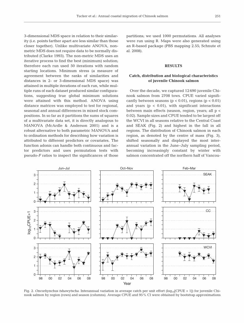
Over the decade, we captured 12 690 juvenile Chi-nook salmon from 2708 tows. CPUE varied signifi-cantly between seasons (p < 0.01), regions (p < 0.01)and years (p < 0.01), with significant interactionsbetween main effects (season, region, years; all p <0.02). Sample sizes and CPUE tended to be largest offthe WCVI in all seasons relative to the Central Coastand SEAK (Fig. 2) and highest in the fall in allregions. The distribution of Chinook salmon in eachregion, as denoted by the centre of mass (Fig. 3),shifted seasonally and displayed the most inter-annual variation in the June−July sampling period,becoming increasingly constant by winter withsalmon concentrated off the northern half of Vancou-

251

Jun–Jul

3

2

1

0

3

2

1

0

3

2

1

0

log 1

0CP

UE

+1

98 00 02 04 06 08

Oct–Nov

98 00 02 04 06 08

Year

Feb–Mar

SEAK

CC

98 00 02 04 06 08

WCVI

Fig. 2. Oncorhynchus tshawytscha. Interannual variation in average catch per unit effort (log10[CPUE + 1]) for juvenile Chi-nook salmon by region (rows) and season (columns). Average CPUE and 95% CI were obtained by bootstrap approximations

Mar Ecol Prog Ser 449: 245–262, 2012

ver Island and the inner channels of SEAK, mostnotably within Sumner Strait. For the most part, as aweighted indice of distribution, the centre of massprovided a reasonable representation of our catches.However, there were 2 main exceptions (SEAK insummer and CC in fall) where the centre of mass waswell off the shelf (Fig. 3). This however is likely anartefact of the calculation.

Fish body size (length; mm) varied significantlybetween years (p < 0.01), seasons (p < 0.01) and re -gions (p < 0.01), with significant interactions betweenmain effects (season, region, years; all p < 0.01). Fishsize was fairly uniform between regions in June toJuly; however, it was generally larger in SEAK andCC than WCVI within each season and year (Fig. 4).In a similar manner, fish dry wt varied significantlybetween years (p < 0.01), seasons (p < 0.01) and re -gions (p < 0.01) with significant interactions betweenmain effects (all p < 0.01). Dry wt (a proxy for lipid

concentration) was also higher in northern samplesthan southern samples within each season and year(Fig. 4).

Trends in mixed-stock compositions

Regional groupings

In summer, Columbia River origin Chinook salmondominated catches in all regions in all years withincreasing proportions from WCVI (average acrossyears 84%) to CC (89%) and to SEAK (98%) (Fig. 5).The WCVI stock formed the majority of the remain-der of fish off WCVI (14%), while Fraser River (4%)and northern BC (5%) were the next largest stocks inCC. In fall, local stocks dominated catches in allregions (e.g. 95% WCVI fish in WCVI; 87% northernBC and Nass and Skeena Rivers fish combined in

252

June-July Oct-Nov Feb-M arch

June-July Oct-Nov Feb-M arch

SEAK

June-July Oct-Nov Feb-M arch

June-July Oct-Nov Feb-M arch

CC

June-July Oct-Nov Feb-M arch

WCVI

June-July Oct-Nov Feb-M archJun–Jul Oct–Nov Feb–Mar

Jun–Jul Oct–Nov Feb–Mar

Jun–Jul Oct–Nov Feb–Mar

Fig. 3. Oncorhynchus tshawytscha. Centre of population mass within sampling regions. Each point represents a single year

Tucker et al.: Annual coastal migration of Chinook salmon

CC; 96% trans-boundary and southeast Alaska fishin SEAK). In all regions, Columbia River fish fell to~1.5% during fall, representing both a proportionaland absolute decline in numerical abundance(Table 2, Fig. 5). In winter, WCVI fish continued todominate catches in WCVI at 65% of the catch. How-ever, there were influxes of Fraser River (10%),Puget Sound (11%), coastal Washington and Oregonfish (6% combined). These represent both increasesin proportion and numerical abundance (Table 2,Fig. 5) from fall when they were all present at <1%.Columbia River fish also increased to comprise 5% ofthe total. In CC, northern BC (43%) and Nass andSkeena Rivers (27%) fish were caught in the highestproportions. The remainder were primarily southeastAlaska (8%) and WCVI (12%) fish. Columbia Riverfish comprised 2% of the total. Trans-boundary andsoutheast Alaska (92%) fish in SEAK continued todominate catches. The remainder was comprised ofpredominantly northern BC and Nass and SkeenaRivers fish.

Sub-regional groupings

To explore whether the grouping of fish into largeregional stocks influenced the impression of consis-tent stock composition as well as look at distributionon a finer scale, we re-examined these at the sub-regional level with 40 sub-populations in total. Themain sub-regional stock groupings varied regionallyand seasonally. All regions were dominated byColumbia River system fish in summer. Snake River-spring/summer fish were found off WCVI to SEAKrepresenting between 35 to 18% respectively of totalChinook salmon catches in summer. With the excep-tion of 4% of fish in fall in SEAK, the proportion ofthis stock declined to <1% in fall and winter samples.Upper Columbia River-spring Chinook salmon rep-resented ~20% of total catches in summer in allregions (Table S1 in the supplement). This stock con-stituted 4% of the catch in SEAK in fall but propor-tions declined to <1% in fall and winter sampling inall other mixed stock compositions. Upper Willamette

253

Leng

th (m

m)

350

250

150

50

29

26

23

20

1729

26

23

20

1729

26

23

20

17

350

250

150

50

350

250

150

50

Jun–Jul

Oct–Nov

Feb–Mar

98 99 00 01 02 03 04 05 06 07 08

Year98 99 00 01 02 03 04 05 06 07 08

% d

ry w

eigh

t

Fig. 4. Oncorhynchus tshawytscha. Box plots of seasonal fork length (mm) and dry wt (as % of total weight) of juvenile Chi-nook salmon in different years. Boxes: west coast of Vancouver Island (WCVI; white) British Columbia (CC; grey), southeast

Alaska (SEAK; black)

Mar Ecol Prog Ser 449: 245–262, 2012

fish constituted 45% of fish in SEAK in summer withvalues of 9 and 5% in CC and WCVI respectively;they constituted <1% in all other samples. Other sub-regional stocks of note (not previously defined) werethe appearance of Skeena Bulkley River fish at 14%in CC in winter, and Unuk River at 7%. In SEAK,Stikine River fish represented 57 and 78% of fish infall and winter catches, while Taku River fish com-prised 9 and 4% in fall and winter; Unuk River fishwere caught at 14 and 6%.

Classification

We performed hierarchical agglomerative clusteranalysis to explore the classifications of the annualand seasonal mixed stock compositions. The result-

ing dendrogram for regional groupings contains 4distinct clusters (Fig. 6) with strong correspondenceto catch region. Fall and winter stock compositionsfor the 3 major geographic regions formed distinctclusters, each of which was dominated by localstocks; that is, the 3 regions were distinct, and withineach region fall and winter stock compositions weresimilar. The final cluster was comprised of summercatches from all regions, where stock compositionwas dominated by Columbia River fish. There were 3exceptions: the 1999 SEAK fall sample grouped withthe summer cluster as they were dominated byColumbia River fish, and the 2001 and 2004 WCVIsummer samples grouped with the WCVI fall andwinter cluster as there were large proportions ofWCVI fish (43 and 66% respectively). This analysisconfirms that regional stocks dominate distribution

254

WCVI

Per

cent

con

trib

utio

n (%

)

98

100

80

60

40

20

0100

80

60

40

20

0100

80

60

40

20

000 02 04 06 08

CC

98 00 02 04 06 08

Year

SEAK

Jun–JulO

ct–Nov

98 00 02 04 06 08

Feb–M

ar

CaliforniaOregonColumbia R.WashingtonPS

Fraser R.ECVIWCVISOBCNOBC

Nass R.Skeena R.QCITransboundarySEAK

Fig. 5. Oncorhynchus tshawytscha. Estimated stock com-position (%) by region (columns) and season (rows) for1998−2008, for 15 regional stocks. PS: Puget Sound,E/WCVI: east/west coast Vancouver Island, QCI: QueenCharlotte Islands, N/SOBC: northern/southern British

Columbia, SEAK: southeast Alaska

Tucker et al.: Annual coastal migration of Chinook salmon

patterns with generally abrupt transitions betweenregions, except in summer when Columbia RiverChinook salmon are migrating north.

The dendrogram from the hierarchical agglomera-tive cluster for the sub-regional groupings containedthe same 4 distinct clusters (Fig. 7) with strong corre-spondence to catch region. There were the same 3exceptions as with the regional stocks. However, the

255

03 F AK 04 W AK 07 W AK 00 F AK 01 F AK 02 F AK 04 F AK 05 F AK

02 W AK 05 W AK 06 W AK 01 W AK 08 F AK 06 F AK 07 F AK

01 W CC 04 F CC

06 W CC 05 W CC 02 F CC 06 F CC 08 F CC 01 F CC 00 F CC 03 F CC

08 W CC 05 F CC 07 F CC 01 W VI 05 W VI 07 F VI 99 F VI 04 F VI 01 F VI 02 F VI 03 F VI 05 F VI 00 F VI 06 F VI

03 W VI 08 F VI 01 S VI 04 S VI

98 F VI 04 W VI 07 W VI 08 W VI 02 W VI 06 W VI

02 S CC 01 S AK 99 F AK

07 S VI 06 S VI 02 S VI 05 S VI

08 S CC 07 S AK 08 S VI

06 S AK 04 S AK 01 S CC 04 S CC 03 S VI

99 S CC 99 S VI 00 S VI

07 S CC 06 S CC

98 S CC 98 S VI

0.0 0.2 0.4 0.6 0.8 1.0

Cluster d

endrogram

Height

Fig. 6. Oncorhynchus tshawytscha. Hierarchical agglomera-tive cluster dendrogram (group-averaging linkages) of re-gional mixed stock compositions. Numbers = abbreviatedyears (e.g. 98 = 1998); S = summer (Jun−Jul), F = fall(Oct−Nov), W = winter (Feb−Mar); VI = west coast of Van-couver Island, CC = Central British Columbia, AK = south-

east Alaska. Blue rectangles highlight main clusters

03 F AK 04 W AK 07 W AK 01 W AK 04 F AK

05 W AK 06 W AK 06 F AK 08 F AK 05 F AK 07 F AK 02 F AK 01 F AK 00 F AK

02 W AK 01 W CC 02 F CC 06 F CC 08 F CC 01 F CC 00 F CC 07 F CC 05 F CC 03 F CC

08 W CC 05 W CC 04 F CC

06 W CC 05 S VI 02 W VI 07 W VI 04 W VI 06 W VI 08 W VI 04 S VI 01 W VI 05 W VI 00 F VI 06 F VI 04 F VI 01 F VI 02 F VI 03 F VI 05 F VI

03 W VI 08 F VI 07 F VI 99 F VI 01 S VI 98 F VI 01 S AK 04 S AK 06 S AK

98 S CC 98 S VI 06 S VI 07 S VI 99 S VI 08 S VI 02 S VI

07 S CC 99 F AK

00 S VI 99 S CC 01 S CC 03 S VI

08 S CC 04 S CC 07 S AK 02 S CC 06 S CC

0.0 0.2 0.4 0.6 0.8 1.0

Cluster d

endrogram

Height

Fig. 7. Oncorhynchus tshawytscha. Hierarchical agglomera-tive cluster dendrogram (group-averaging linkages) of sub-

regional mixed stock compositions. Legend as in Fig. 6

Mar Ecol Prog Ser 449: 245–262, 2012

2005 sample from summer in WCVI fell out on itsown. Sample size (n = 7) was small and dominated byUpper Columbia River-summer/fall fish.

Ordination

Variation in mixed stock composition was exploredby ordination using non-metric MDS and confirmedthe patterns observed in cluster analysis as discussedabove. The non-metric MDS analysis of mixed stockrepresented the data reasonably well (Clarke & War-wick 2001) in 2 dimensions (2D stress = 0.14; Fig. 8)and resulted in 4 non-overlapping groups of mixedstocks in common catch regions. This was improvedin 3 dimensions (3D stress = 0.06). In Fig. 8, we havealso superimposed the resultant cluster configurationin the non-metric MDS plot (Clarke & Warwick 2001,Oksanen et al. 2011); group delineation proved to becongruent between the 2 techniques. For the sub-regional mixed stock groupings, the 2D non-metricMDS stress was 0.17, suggesting that the test perfor-mance was fair (Clarke & Warwick 2001), also result-ing in 4 distinct groups. Again, this was improved in3 dimensions (3D stress = 0.09).

Analysis of variance

Examining regional mixed-stock compositions withANOVA using the Bray-Curtis distance matrices, wefound significant differences between regions (p <0.01) and seasons (p < 0.01), but no effect of year (p =0.30). Similarly, for sub-regional groupings, we foundsignificant differences between regions (p < 0.01)and seasons (p < 0.01), but no effect of year (p = 0.21).

DISCUSSION

No study to date has been able to documentannual changes in stock composition and migrationbehaviour of juvenile salmon due to both small sam-ple sizes (Trudel et al. 2009, Tucker et al. 2009) orthe inability to identify individual stocks (e.g. Hartt& Dell 1986). In this study, sample sizes were largeenough to evaluate annual changes in migrationbehaviour, owing both to extensive sampling effortand the application of microsatellites for individualstock identification. There may of course be somesmaller scale regional patterns in movement anddistribution masked by the aggregation of fish intolarge sampling regions. Specific trajectories maychange between years. However, the overarchingpatterns were consistent despite the large variationsin ocean conditions encountered by salmon over thetime period of our study: coastal residency of localstocks in their first year at sea except for southernyearling fish (Columbia River and coastal USA),which moved quickly into waters north of WCVI insummer.

Variable conditions in the North Pacific Ocean, aswell as large overall shifts in ocean regimes and con-sequent shifts in primary and secondary productionhave been extensively documented during the pe -riod of this study (e.g. DFO 2009). In addition, previ-ous work has outlined correlations between variousenvironmental conditions and the presence, abun-dance, condition and survival of Chinook salmon(Fisher et al. 2007, Bi et al. 2007, 2011a, Wells etal. 2008, MacFarlane 2010, Peterson et al. 2010,Duffy & Beauchamp 2011). Our objective was not tore-establish those, but to extend our understandingby evaluating the consistency in regional and sea-sonal stock compositions over a decade that sawlarge changes in ocean conditions. We demonstratethat the distribution and abundance, as well as thesize and condition of fish, varied between years on aseasonal basis in all regions. No doubt these areinfluenced by specific environmental conditions and

256

–0.5

0.5

0

–0.5

0 0.5

Dimension 1

Dim

ensi

on 2

CCSEAKWCVI

Fig. 8. Oncorhynchus tshawytscha. Non-metric multidimen-sional scaling ordination plot of regional mixed stock com-positions (2D stress = 0.14). Mixed stock groupings coded bycatch region. Dashed lines: resultant cluster groupings fromhierarchical agglomerative cluster analysis. WCVI: westcoast Vancouver Islands, CC: central British Columbia,

SEAK: southeast Alaska

Tucker et al.: Annual coastal migration of Chinook salmon

food web processes that have been previously out-lined. Changes in CPUE potentially reflect changesin marine survival, although it is difficult to accountfor differences in freshwater recruitment and smoltproduction between years given the lack of informa-tion on smolt outputs for the vast majority of stocks(Pacific Salmon Commission 2009). At the very least,size and condition have important consequences forsurvival (Beamish & Mahnken 2001, Moss et al. 2005,Duffy & Beauchamp 2011, Farley et al. 2011). How-ever, we observed no response in terms of large shiftsin stock specific distributions within that first year ofmarine life (i.e. across all seasons). Stock compositionwas similar between years suggesting migration pat-terns for all stocks remain consistent despite largefluctuations in the marine environment. It is possiblehowever, that under certain conditions, fish from allstocks are moving undetected beyond our samplingarea in a synchronous and rapid manner that wouldnot be reflected in our mixed stocked results.Although the scope of our sampling was large, it wasnot large enough to address this possibility, whichhas different implications for plasticity.

The similarity in regional stock compositions be -tween years at both the regional and sub-regionalstock level was demonstrated by classification andordination procedures. Fall and winter stock compo-sitions from each catch region formed 3 distinct clus-ters, each dominated by local stocks. The final clusterwas comprised of summer catches from all regions,where stock composition was dominated by Colum-bia River yearling fish. There were 3 principal out-liers to this pattern: the 1999 SEAK fall samplegrouped with the summer cluster as they were domi-nated by Columbia River fish, and the 2001 and 2004WCVI summer samples grouped with the WCVI falland winter cluster as there were large proportions ofWCVI fish (43 and 66% respectively). Two of thesediscrepancies can be explained by different sam-pling location and effort. In fall 1999, at the begin-ning of the program, we did not sample the insidepassages of SEAK. This is where the vast majority(~99%) of Chinook salmon have been caught inSEAK and are overwhelmingly trans-boundary fishand other northern stocks (98% of inside fish total).Columbia River fish tend to be caught in outsidewaters (5 out of 9 Chinook salmon caught in outsidewaters, or 55%) and very rarely inside (0.6% of total).Given that the 1999 fall sample size was small and aswe fished only on the continental shelf rather than inthe straits and inlets, this sample was likely skewedin favour of Columbia River fish. In summer, werarely sampled the inside inlets and sounds of WCVI.

However, in 2004 and 2007, we did and subsequentlycaught 81 (n = 73) and 100% (n = 7) WCVI fishrespectively. However, in 2004 this inside catch waslarge and comprised 66% of the total catch; in 2007the catch represented only 10% of the total. How-ever, in both these cases, fishing inside waters likelyskewed the catches towards WCVI fish. In 2001 wedid not fish the inside waters but almost half thecatch was made up of WCVI fish. Since there was noidentifiable shift in location or timing of sampling, itappears this represents an early emergence of WCVIfish onto the shelf as we have never observed themhere in other years. It also appeared to be a year oflow abundance of Columbia River fish off WCVI butthis was not a general trend across the other sam-pling areas, suggesting that perhaps survival condi-tions were very poor that year and/or fish migratednorth faster.

Even at the level of sub-regional stocks, patternsremained consistent among years. In summer, Co -lum bia River origin Chinook salmon dominated cat -ches coast wide, representing >90% of all Chinooksalmon, suggesting a rapid northward migration formany fish. The vast majority of these were spring-runChinook salmon that moved quickly into watersnorth of Vancouver Island, including southeastAlaska. The primary stocks were Snake River−spring/summer, Upper Columbia River−spring andUpper Willamette. These tend to be yearling smoltssuggesting a component of life history variation inmigration pattern (Trudel et al. 2009, Tucker et al.2011). However, there were some Chinook salmonfrom Upper Columbia summer−fall runs that werefound off WCVI in significant proportions, thoughnone were identified north of Vancouver Island. Incontrast, these tend to be sub-yearling smolts. How-ever, the vast majority of sub-yearling smolts fromother Columbia River stocks are first caught in thesewaters in fall (Tucker et al. 2011). This would suggestthat, with respect to migration patterns, at least forUpper Columbia River fish, there may be some affin-ity to the river of origin and ESU (Waples et al. 2004)

Columbia River fish subsequently became minorcomponents in catches in fall and winter as propor-tions declined to <20% of Chinook salmon caught.The majority of these fish were fall-run, sub-yearlingChinook salmon primarily from the Upper ColumbiaRiver. In general, fall-run and spring-run Chinookdisplay opposing migration patterns with either aperiod of coastal residency or rapid migration respec-tively (Trudel et al. 2009, Tucker et al. 2011, J. Fisherunpubl.). Given the propensity of juvenile Chinooksalmon for local residency in the first year of marine

257

Mar Ecol Prog Ser 449: 245–262, 2012

life (current study, Murphy et al. 2009, Trudel et al.2009, Tucker et al. 2011), some sub-regional popula-tions were likely over or under-represented in thebroad regional mixed-stock analysis particularly atthe edges of our sampling area. For example inSEAK, our sample is weighted by Stikine River fish,even though escapements are on the same order asthe Taku River (Pacific Salmon Commission 2009).Similarly, based on the small escapements of UnukRiver fish, these are likely over-represented in oursample (Pacific Salmon Commission 2009). This islikely due to concentration of our fishing effort in thesouthern portion of SEAK in closer proximity to theStikine and Unuk Rivers.

Little inter-annual stock-specific change in marinedistributions, despite changes in ocean conditions,would suggest that Chinook salmon distributions areprimarily driven by genetic control of migration(Bran non & Setter 1989, Kallio-Nyberg & Ikonen1992) than by either local environmental conditions(Hodgson et al. 2006) or opportunistic foragingopportunities (Healey 2000). Conversely, the differ-ences in ocean conditions observed during this timespan were not large enough to effect a measurablechange in stock specific distributions in spite of thefact that growth, condition (present study), and sur-vival (Pacific Salmon Commission 2009) all variedsubstantially over this decade. This seems unlikelyhowever given that what would generally be consid-ered ‘extreme’ climatic events were observed overthis timeframe. For example, a major El Niño warm-ing event in 1998 was followed by near normal con-ditions in 1999 with moderate La Niña conditions in2000. These moderate La Niña conditions persistedin 2001 in the northeast Pacific and coastal BritishColumbia. However, in 2002 weak El Niño conditionsoccurred in the second half of the year. The weak ElNiño of 2002 to 2003 set up anomalously warm seasurface temperatures to mid 2003 when the oceansurface waters cooled somewhat, returning to moreaverage temperatures until early 2004. In May 2004,the coastal ocean waters off British Columbia wereabove average in temperature; these were main-tained into 2006 in the entire northeast Pacific(Mackas et al. 2006). However, except for a briefwarm period in summer, ocean waters were coolerthan normal through 2007 and into 2008. Thesecooler temperatures were associated with La Niñaconditions in spring and autumn 2007. Despite con-tinuing increases in overall global water tempera-tures, the waters off the Pacific coast of Canada in2008 were the coldest in 50 yr, and the coolingextended far into the Pacific Ocean and south along

the American coast. Shifts in zooplankton abun-dances and species assemblages were coincidentwith the large scale changes in ocean temperature(DFO 2009). In 1998, indeed during the previousdecade, zooplankton assemblages in the NE Pacificwere dominated by ‘southerly’ copepod fauna (DFO2000). In 1999, following the strong La Niña thatbegan in late 1998 in the equatorial Pacific, the con-centrations of all of the major zooplankton taxaswung sharply back toward or past their long termaverage levels to more boreal and sub-arctic assem-blages into 2002. Zooplankton communities againreturned to ‘cool-ocean’ species in 2007; this trendcontinued into 2008. This is in contrast to the previ-ous 3 yr during which warm water, southern speciespredominated.

There is, of course, a further question as to whetherwidespread and stable marine distributions may existin other Pacific salmon and other fish species, andmay be a universal evolutionary response to dynamicmarine environments. Chinook salmon appear to beunique in their migration strategy of coastal resi-dence as many fish do not appear to leave the shelfuntil after their second summer at sea (Murphy et al.2009, Trudel et al. 2009, Tucker et al. 2011). In con-trast, juvenile sockeye Oncorhynchus nerka, coho,pink O. gorbucha and chum salmon O. keta arethought to leave coastal shelf waters between falland the onset of spring (Fisher et al. 2007, Morris etal. 2007, Tucker et al. 2009) or possibly earlier(M. Trudel unpubl. data). Given the rapid movementof juvenile sockeye and coho salmon (species forwhich we have stock-specific data), compared to theresident pattern of sub-yearling Chinook salmon, it isunlikely that mixed-stock compositions per se wouldremain constant as in the case here. However, byexamining the composite distribution of individualsfrom particular stocks separately, it is clear thatstocks consistently display similar migration patternsfrom year to year (S. Tucker unpubl. data). For exam-ple, over a 10 yr period, Fraser River sockeye salmonstocks left the Strait of Georgia in spring/early sum-mer via a northern route though Johnstone Strait intoQueen Charlotte Sound. The exception was HarrisonRiver fish, which migrated via the southern routethrough Juan de Fuca continuing north off the WestCoast of Vancouver at some point in the winter(Tucker et al. 2009, S. Tucker unpubl. data). So whilethe specific timing of migration might vary betweenyears, and there may be very local effects on survivalfor specific stocks resulting in different regionalmixed-stock compositions, the patterns displayed areconsistent from one year to the next.

258

Tucker et al.: Annual coastal migration of Chinook salmon

Few studies have been successful in linking the ef-fects of ocean conditions on Chinook salmon produc-tion (e.g. Beamish et al. 1995, Ruggerone & Goetz2004, Scheuerell & Williams 2005, Wells et al. 2006,2007, 2008). The results of such analyses are often dif-ficult to interpret since they rely on large-scaleclimate indices that may not always reflect the veryspecific areas where individual stocks of Chinooksalmon seem to be resident. The results outlined hereand in Trudel et al. (2009) underline the importance ofconsidering relevant spatial and temporal scales forassessing the effects of ocean conditions on Pa cificsalmon, particularly since there is increasing evidencethat recruitment is potentially set within the first yearof marine life (Pearcy 1992, Beamish & Mahnken2001, Beamish et al. 2004, Cross et al. 2009, Duffy &Beauchamp 2011). Our analyses indicate that relevantspatial and temporal scales vary with stock and lifehistory. Effects of ocean conditions on fall Chinooksalmon are expected to be manifested at a local scalefor coastal stocks (i.e. within 200 to 400 km of the natalriver), compared to the scale of the northern CaliforniaCurrent (i.e. California/Oregon to the west coast ofVancouver Island) for southern US origin fall fish.Even broader and more complex spatial and temporalscales must be considered for southern US spring Chi-nook salmon, as ocean conditions vary among bothregions and months, and stocks are distributed acrossthe shelf. The limited inter-annual variation in marinedistributions evident for both juvenile Chinook salmonin the present study and adult Chinook salmon(Weitkamp 2010), despite highly variable ocean con-ditions, suggests that poor ocean conditions mayresult in poor survival rather than adaptive alterationsin movement and distribution. If this is true, variousscenarios of climate change and accompanying in-creases in ocean temperatures with unfavourablegrowing conditions do not bode well particularly forsouthern stocks of Chinook salmon. These essentiallypredict that these stocks will increasingly be morelikely to encounter areas of low growth and survival(however see Sydeman et al. 2011). If so, then themarine survival and resulting conservation status ofindividual salmon stocks may be strongly determinedby their entry point into the ocean, which discreteoceanographic regions they encounter, and their du-ration of residency within each region.

Acknowledgements. We thank the crews of the CCGS ‘W.E.Ricker’, FV ‘Ocean Selector’, FV ‘Frosti’ and FV ‘VikingStorm’ and the numerous scientists and technicians for theirassistance with the field work and laboratory analysis, theBonneville Power Administration and Fisheries and OceansCanada for their financial support.

LITERATURE CITED

Båmstedt U (1986) Chemical composition and energy content. In: Corner EDS, O’Hara SCM (eds) The biologi-cal chemistry of marine copepods. Clarendon, Oxford,p 1–58

Batten SD, Freeland HJ (2007) Plankton populations at thebifurcation of the North Pacific Current. Fish Oceanogr16: 536−646

Batten S, Hyrenbach D, Sydeman W, Morgan K, Henry M,Yen P, Welch DW (2006) Characterising meso-marineecosystems of the North Pacific. Deep-Sea Res II 53: 270−290

Beacham TD, Candy JR, Jonsen KL, Supernault J and others(2006a) Estimation of stock composition and individualidentification of Chinook salmon across the Pacific Rimby use of microsatellite variation. Trans Am Fish Soc 135: 861−888

Beacham TD, Jonsen KL, Supernault J, Wetklo M, Deng L,Varnavskaya N (2006b) Pacific Rim population structureof Chinook salmon as determined from microsatelliteanalysis. Trans Am Fish Soc 135: 1604−1621

Beamish RJ, Mahnken C (2001) A critical size and periodhypothesis to explain natural regulation of salmon abun-dance and the linkage to climate and climate change.Prog Oceanogr 49: 423−437

Beamish RJ, Riddell BE, Neville CM, Thomson BL, Zhang Z(1995) Declines in Chinook salmon catches in the Straitof Georgia in relation to shifts in the marine environ-ment. Fish Oceanogr 4: 243−256

Beamish RJ, McFarlane GA, Schweigert J (2001) Is the pro-duction of coho salmon in the Strait of Georgia linked tothe production of Pacific Herring? In: Funk F, BlackburnJ, Hay D, Paul AJ, Stephenson R, Toresen R, Witherell D(eds) Herring: expectations for a new millenium. Univer-sity of Alaska Sea Grant, AK-SG-01-04, Fairbanks, AK,p 37−50

Beamish RJ, Sweeting RM, Neville CE, Poier K (2002) A cli-mate related explanation for the natural control of Pacificsalmon abundance in the first marine year. NPAFC Tech-nical Report No. 4

Beamish RJ, Mahnken C, Neville CM (2004) Evidence thatreduced early marine growth is associated with lowermarine survival of coho salmon. Trans Am Fish Soc 133: 26−33

Bi H, Ruppel R, Peterson WT (2007) Modeling the pelagichabitat of salmon off the Pacific Northwest (USA) coastusing logistic regression. Mar Ecol Prog Ser 336: 249−265

Bi H, Ruppel RE, Peterson WT, Casillas E (2008) Spatial dis-tribution of ocean habitat of yearling Chinook (Onco -rhynchus tshawytscha) and coho (Oncorhynchus ki -sutch) salmon off Washington and Oregon, USA. FishOceanogr 17: 463−476

Bi H, Peterson WT, Lamb J, Casillas E (2011a) Copepods andsalmon: characterizing the spatial distribution of juvenilesalmon along the Washington and Oregon coast, USA.Fish Oceanogr 20: 125−138

Bi H, Peterson WT, Strub T (2011b) Transport and coastalzooplankton communities in the northern California Cur-rent system. Geophys Res Lett 38: L12607. doi:10.1029/2011GL047927

Brannon E, Setter A (1989) Marine distribution of a hatcheryfall Chinook salmon population. In: Brannon EL, JonssonB (eds) Proc Salmonid Migration and Distribution Symp.University of Washington, Seattle, WA, p 63−69

259

Mar Ecol Prog Ser 449: 245–262, 2012

Brodeur RD, Boehlert GW, Casillas E, Eldridge MB and others (2000) A coordinated research plan for estuarineand ocean research on Pacific salmon. Fisheries(Bethesda, Md) 25: 7−16

Brodeur RD, Fisher JP, Teel DJ, Emmett RL, Casillas E,Miller TW (2004) Juvenile salmonid distribution, growth,condition, origin, and environmental and species associ-ations in the Northern California Current. Fish Bull 102: 25−46

Clarke KR (1993) Non-parametric multivariate analysesof changes in community structure. Aust J Ecol 18: 117−143

Clarke KR, Warwick RM (2001) Changes in marine commu-nities: an approach to statistical analysis and interpreta-tion, 2nd edn. PRIMER-E, Plymouth Marine Laboratory,Plymouth

Cross AD, Beauchamp DA, Moss JH, Myers KW (2009)Interannual variability in early marine growth, size-selective mortality, and marine survival for PrinceWilliam Sound pink salmon. Mar Coast Fish: Dyn Man-age Ecosyst Sci 1: 57−70

DFO (2000) 1999 Pacific region state of the ocean. DFO CanSci Advis Sec Sci Advis Rep 2000/01

DFO (2009) State of the Pacific Ocean 2008. DFO Can SciAdvis Sec Sci Advis Rep 2009/030

Duffy EJ, Beauchamp DA (2011) Rapid growth in the earlymarine period improves the marine survival of Chinooksalmon (Oncorhynchus tshawytscha) in Puget Sound,Washington. Can J Fish Aquat Sci 68: 232−240

Farley EV, Starovoytov A, Naydenko S, Heintz R and others(2011) Implications of a warming eastern Bering Sea forBristol Bay sockeye salmon. ICES J Mar Sci 68:1138–1146

Fisher J, Trudel M, Ammann A, Orsi JA and others(2007) Comparison of the coastal distributions and abun-dances of juvenile Pacific salmon from Central Californiato the Northern Gulf of Alaska. In: Grimes CB, BrodeurRD, Haldorson LJ, McKinnell SM (eds) The ecology ofjuvenile salmon in northeast Pacific Ocean: regionalcomparisons. Am Fish Soc Symp 57, Bethesda, MD,p 31−80

Fritz H, Said S, Weimerskirch H (2003) Scale-dependenthierarchical adjustments of movement patterns in a long-range foraging seabird. Proc Biol Sci 270: 1143−1148

Gargett AE (1997) The optimal stability ‘window’: a mecha-nism underlying decadal fluctuations in North Pacificsalmon stocks? Fish Oceanogr 6: 109−117

Hare SR, Mantua NJ, Francis RC (1999) Inverse productionregimes: Alaskan and West Coast Pacific salmon. Fish-eries 24: 6−14

Hartt AC, Dell MB (1986) Early oceanic migrations andgrowth of juvenile Pacific salmon and steelhead trout.Bull Int North Pac Fish Comm 46: 1−105

Healey MC (1991) Life history of Chinook salmon (Onco -rhynchus tshawytscha). In: Groot C, Margolis L (eds)Pacific salmon life histories. University of British Colum-bia Press, Vancouver, p 311−394

Healey MC (2000) Pacific salmon migrations in a dynamicocean. In: Harrison PJ, Parsons TR (eds) Fisheriesoceanography: an integrative approach to fisheries ecology and management. Blackwell Science, Oxford,p 29−54

Hickey BM, Banas NM (2008) Why is the northern end of theCalifornia Current System so productive? Oceanography21: 90−107

Hodgson S, Quinn TP, Hilborn R, Francis RC, Rogers DE(2006) Marine and freshwater climatic factors affectinginterannual variation in the timing of return migration tofresh water of sockeye salmon (Oncorhynchus nerka).Fish Oceanogr 15: 1−24

Hollowed A, Wooster WS (1992) Variability of winter oceanconditions and strong year classes of northeast Pacificgroundfish. ICES Mar Sci Symp 195: 433−444

Hurst TP (2007) Causes and consequences of winter mortal-ity in fishes. J Fish Biol 71: 315−345

Kallio-Nyberg I, Ikonen E (1992) Migration pattern of twosalmon stocks in the Baltic Sea. ICES J Mar Sci 49: 191−198

Legendre P, Legendre L (1998) Numerical ecology, 2nd Eng-lish edn. Elsevier Press, New York, NY

MacFarlane RB (2010) Energy dynamics and growth of Chinook salmon (Oncorhynchus tshawytscha) from theCentral Valley of California during the estuarine phaseand first ocean year. Can J Fish Aquat Sci 67: 1549−1565

Mackas DL, Peterson WT, Zamon JE (2004) Comparisons ofinterannual biomass anomalies of zooplankton commu-nities along the continental margins of British Columbiaand Oregon. Deep-Sea Res II 51: 875−896

Mackas DL, Peterson WT, Ohman MD, Lavaniegos BE(2006) Zooplankton anomalies in the California Currentsystem before and during the warm ocean conditions of2005. Geophys Res Lett 33: L22S07. doi:10.1029/ 2006 GL027930

Mackas DL, Batten S, Trudel M (2007) Time series of theNortheast Pacific effects on zooplankton of a warmerocean: recent evidence from the Northeast Pacific. ProgOceanogr 75: 223−252

Mantua NJ, Hare SR, Zhang Y, Wallace JM, Francis RC(1997) A Pacific decadal climate oscillation with impactson salmon. Bull Am Meteorol Soc 78: 1069−1079

McArdle BH, Anderson MJ (2001) Fitting multivariate mod-els to community data: a comment on distance-basedredundancy analysis. Ecology 82: 290−297

Morris JFT, Trudel M, Thiess ME, Sweeting RM and others(2007) Stock-specific migrations of juvenile coho salmonderived from coded-wire tag recoveries on the continen-tal shelf of Western North America. In: Grimes CB,Brodeur RD, Haldorson LJ, McKinnell SM (eds) The ecol-ogy of juvenile salmon in northeast Pacific Ocean: regional comparisons. Am Fish Soc Symp 57, Bathesda,MD, p 81−104

Moss JH, Beauchamp DA, Cross AD, Myers KW, Farley EVJr, Murphy JM, Helle JH (2005) Evidence for size- selective mortality after the first summer of ocean growthby pink salmon. Trans Am Fish Soc 134: 1313−1322

Mueter FJ, Ware DM, Peterman RM (2002) Spatial correla-tion patterns in coastal environmental variables and sur-vival rates of salmon in the north-east Pacific Ocean. FishOceanogr 11: 205−218

Murphy JM, Templin WD, Farley Jr, EV, Seeb JE (2009)Stock-structured distribution of western Alaska andYukon juvenile Chinook salmon (Oncorhynchus tsha -wytscha) from United States BASIS surveys, 2002−2007.North Pac Anadromous Fish Comm Bull 5: 51−59

Neaves PI, Wallace CG, Candy JR, Beacham TD (2005)CBayes: computer program for mixed stock analysis ofallelic data. Version 4.01, available at www.pac.dfo-mpo.gc.ca/sci/mgl/Cbayes_e.htm

Oksanen J, Blanchet FG, Kindt R, Legendre P and others(2011). vegan: Community Ecology Package. R package

260

Tucker et al.: Annual coastal migration of Chinook salmon

version 1.17-8, available at http: //CRAN.R-project.org/package=vegan

Orsi JA, Jaenicke HW (1996) Marine distribution and originof prerecruit Chinook salmon, Oncorhynchus tsha -wytscha, in Southeastern Alaska. Fish Bull 94: 482−497

Orsi JA, Harding JA, Pool SS, Brodeur RD and others (2007)Epipelagic fish assemblages associated with juvenilePacific salmon in neritic waters of the California Currentand the Alaska Current. In: Grimes CB, Brodeur RD, Hal-dorson LJ, McKinnell SM (eds) The ecology of juvenilesalmon in northeast Pacific Ocean: regional comparisons.Am Fish Soc Symp 57, Bethesda MD, p 105−156

Pacific Salmon Commission (2009) Annual report of catchesand escapements. Joint Chinook Tech Comm RepTCCHINOOK (09)-1

Pearcy WG (1992) Ocean ecology of North Pacificsalmonids. University of Washington Press, Seattle, WA

Pella J, Masuda M (2001) Bayesian methods for analysis ofstock mixtures from genetic characters. Fish Bull 99: 151−167

Pennington M (1996) Estimating the mean and variance ofhighly skewed marine data. Fish Bull 94: 498−505

Peterson W (2009) Copepod species richness as an indicatorof long term changes in the coastal ecosystem of thenorthern California Current. CCOFI Rep 50: 73−81

Peterson WT, Morgan CA, Fisher JP, Casillas E (2010)Ocean distribution and habitat associations of yearlingcoho (Oncorhynchus kisutch) and Chinook (O. tsha wyt -scha) salmon in the northern California Current. FishOceanogr 19: 508−525

Quinn TP, Dickerson BR, Vøllestada LA (2005) Marine sur-vival and distribution patterns of two Puget Sound hatch-ery populations of coho (Oncorhynchus kisutch) and Chi-nook (Oncorhynchus tshawytscha) salmon. Fish Res 76: 209−220

R Development Core Team (2011) R: a language and envi-ronment for statistical computing. R Foundation for Sta-tistical Computing, Vienna, available at www.r-project.org

Rechisky ER, Welch DW, Porter AD, Jacobs MC, LadouceurA (2009) Experimental measurement of hydrosystem-induced mortality in juvenile Snake River spring Chi-nook salmon using a large-scale acoustic array. Can JFish Aquat Sci 66: 1019−1024

Ruggerone GT, Goetz FA (2004) Survival of Puget SoundChinook salmon (Oncorhynchus tshawytscha) in res -ponse to climate-induced competition with pink salmon(Oncorhynchus gorbuscha). Can J Fish Aquat Sci 61: 1756−1770

Satterfield FR, Finney BP (2002) Stable isotope analysis ofPacific salmon: insight into trophic status and oceano-graphic conditions over the last 30 years. Prog Oceanogr53: 231−246

Scheuerell MD, Williams JG (2005) Forecasting climate-induced changes in the survival of Snake River spring/summer Chinook salmon (Oncorhynchus tshawytscha).Fish Oceanogr 14: 448−457

Schnute JT, Boers NM, Haigh R, Couture-Beil A (2008) PBSmapping 2.55: user’s guide revised. Can Tech Rep FishAquat Sci 2549: 1−118

Smith SJ (1988) Evaluating the efficiency of the delta-distribution mean estimator. Biometrics 44: 485−493

Strub PT, James C (2002) Altimeter-derived surface circula-tion in the large-scale NE Pacific Gyres. Part 1: seasonalvariability. Prog Oceanogr 53: 163−183

Sydeman WJ, Thompson SA, Field JC, Peterson WT andothers (2011) Does positioning of the North Pacific Cur-rent affect downstream ecosystem productivity? Geo-phys Res Lett 38: L12606. doi:10.1029/2011GL047212

Teel DJ, Milner GB, Winans GA, Grant WS (2000) Geneticpopulation structure and origin of life history types inChinook salmon in British Columbia, Canada. Trans AmFish Soc 129: 194−209

Trudel M, Tucker S, Morris JFT, Higgs DA, Welch DW(2005) Indicators of energetic status in juvenile cohosalmon and Chinook salmon. N Am J Fish Manage 25: 374−390

Trudel M, Thiess ME, Bucher C, Farley EV Jr and others(2007) Regional variation in the marine growth andenergy accumulation of juvenile Chinook salmon andcoho salmon along the west coast of North America. In: Grimes CB, Brodeur RD, Haldorson LJ, McKinnell SM(eds) The ecology of juvenile salmon in northeast PacificOcean: regional comparisons. Am Fish Soc Symp 57,Bethesda, MD, p 205−232

Trudel M, Fisher J, Orsi JA, Morris JFT and others (2009)Distribution and migration of juvenile Chinook salmonderived from coded-wire tag recoveries along the conti-nental shelf of western North America. Trans Am FishSoc 138: 1369−1391

Tucker S, Trudel M, Welch DW, Candy JR and others (2009)Seasonal stock-specific migration of juvenile sockeyesalmon along the west coast of North America; implica-tions for growth. Trans Am Fish Soc 138: 1458−1480

Tucker S, Trudel M, Welch DW, Morris JFT, Candy JR, Wal-lace C, Beacham TD (2011) Life-history and seasonalstock-specific ocean migration of juvenile Chinook sal -mon. Trans Am Fish Soc 140:1101–1119

Turchin P (1998) Quantitative analysis of movement: mea-suring and modeling population redistribution in plantsand animals. Sinauer Associates, Sunderland, MA

Waples RS, Teel DJ, Myers JM, Marshall AR (2004) Life- history divergence in Chinook salmon: historic contin-gency and parallel evolution. Evolution 58: 386−403

Ware DM, McFarlane GA (1989) Fisheries productiondomains in the Northeast Pacific Ocean. Can Spec PublFish Aquat Sci 108: 359−379

Ware DM, Thomson RE (2005) Bottom-up ecosystem trophicdynamics determine fish production in the northeastPacific. Science 308: 1280−1284

Weitkamp L (2010) Marine distributions of Chinook salmonfrom the West Coast of North America determined bycoded wire tag recoveries. Trans Am Fish Soc 139: 147−170

Weitkamp L, Neely K (2002) Coho salmon (Oncorhynchuskisutch) ocean migration patterns: insight from marinecoded-wire tag recoveries. Can J Fish Aquat Sci 59: 1100−1115

Welch DW, Parsons TR (1993) δ13C-δ15N values as indicatorsof trophic position and competitive overlap for Pacificsalmon (Oncorhynchus spp.). Fish Oceanogr 2: 11−23

Welch DW, Melnychuk MC, Rechisky EL, Porter AD andothers (2009) Freshwater and marine migration and sur-vival of endangered Cultus Lake sockeye salmon smoltsusing POST, a large-scale acoustic telemetry array. CanJ Fish Aquat Sci 66: 736−750

Welch DW, Melnychuk MC, Payne J, Rechisky EL and others (2011) In situ measurement of coastal ocean move-ments and survival of juvenile Pacific salmon. Proc NatlAcad Sci USA 108: 8708−8713

261

Mar Ecol Prog Ser 449: 245–262, 2012

Wells BK, Grimes CB, Field JC, Reiss CS (2006) Covariationbetween the average lengths of mature coho (Onco -rhynchus kisutch) and Chinook salmon (Oncorhynchustshawytscha) and the ocean environment. Fish Oceanogr15: 67−79

Wells B, Grimmes CB, Waldvogel J (2007) Quantifying theeffects of wind, upwelling, curl, sea surface temperatureand sea level height on growth and maturation of a California Chinook salmon (Oncorhynchus tshawytscha)population. Fish Oceanogr 16: 363−382

Wells BK, Grimes CB, Sneva JG, McPherson S, WaldvogelJB (2008) Relationships between oceanic conditions andgrowth of Chinook salmon (Oncorhynchus tshawytscha)from California, Washington, and Alaska, USA. FishOceanogr 17: 101−125

Willette TM, Cooney RT, Patrick V, Mason DM, Thomas GL,Scheel TD (2001) Ecological processes influencing mor-tality of juvenile pink salmon (Oncorhynchus gorbuscha)in Prince William Sound, Alaska. Fish Oceanogr10(Suppl 1): 14−41

Withler RE, Le KD, Nelson RJ, Miller KM, Beacham TD(2000) Intact genetic structure and high levels ofgenetic diversity in bottlenecked sockeye salmon(Onco r hyn chus nerka) populations of the Fraser River,British Columbia, Canada. Can J Fish Aquat Sci 57: 1985−1998

Zamon JE, Welch DW (2005) Rapid shift in zooplanktoncommunity composition on the northeast Pacific shelfduring the 1998−1999 El Niño−La Niña event. Can J FishAquat Sci 62: 133−144

262

Editorial responsibility: Nicholas Tolimieri, Seattle, Washington, USA

Submitted: August 11, 2011; Accepted: November 23, 2011Proofs received from author(s): February 23, 2012