an#investigation#ofantennapatterns...
TRANSCRIPT

An Investigation of Antenna Patterns for the CETB
David G. Long, BYU Version 1.1 2 Mar 2015
Abstract
This report discusses the use and modeling of sensor antenna patterns for estimating the spatial response function of radiometer measurements for two of the sensors used in the Calibrated Passive Microwave Daily EASE-Grid 2.0 Brightness Temperature ESDR (CETB). Both simulated and actual antenna patterns are studied. The relationship of the antenna pattern to the spatial response function is derived and explored. A common model (a Gaussian function) is compared to the antenna pattern and spatial response function. The model adequately represents the mainlobe of the pattern and response function, though it does not model the rolloff of sidelobes well. Using a second Gaussian (termed a dual-Gaussian model) improves the fit. When considering the difficulties and uncertainties in trying to use measured antenna patterns, and in light of the relative insensitivity of the CETB reconstruction processing to errors in the spatial response function, we conclude that the simple Gaussian approximation is adequate for modeling the response function in the CETB reconstruction processing.
1 Introduction The goal of the Calibrated Passive Microwave Daily EASE-Grid 2.0 Brightness
Temperature ESDR (CETB) project (Brodzik and Long, 2014) is to produce both low-noise gridded data and enhanced-resolution data products. The former is based on “drop in the bucket” (DIB) gridding which requires no information about the sensor’s measurement spatial response function (SRF). However, the latter uses reconstruction techniques to enhance the spatial resolution and requires knowledge of the SRF for each measurement. The SRF is different for each sensor channel and varies over the measurement swath. Due to variations in the measurement geometry around the orbit, the SRF is also orbit position dependent. For microwave radiometers the key factor affecting the SRF is projection of the antenna pattern on to the surface and the temporal integration period used to collect estimates of the brightness temperature (TB). The purpose of this report is to explore how the antenna pattern affects the SRF and how the SRF should be modeled for CETB processing.

3/2/15 Page 2 of 55
2 Relation of the Antenna Pattern to the SRF This section provides a brief background and describes how the SRF is related to
the antenna pattern.
2.1 Background Theory Microwave radiometers measure the thermal emission, sometimes called the
Plank radiation, radiating from natural objects (Ulaby and Long, 2014). In a typical radiometer, an antenna is scanned over the scene of interest and the output power from the carefully calibrated receiver is measured as a function of scan position. The reported signal is a temporal average of the filtered received signal power.
The observed power is related to the receiver gain and noise figure, the antenna loss, the physical temperature of the antenna, the antenna pattern, and the scene brightness temperature. In simplified form, the output power PSYS of the receiver can be written as (Ulaby and Long, 2014)
PSYS = k TSYS B (1)
where k = 1.38×10⁻²⁸ is Boltzmann's constant in W/(K Hz), B is the receiver bandwidth in Hz, and TSYS is the system temperature in K defined as:
TSYS = ηl TA + (1 - ηl) Tp + (L - 1) Tp + L TREC (2)
where ηl is the antenna loss efficiency, Tp is the physical temperature of the antenna and waveguide feed, L is waveguide loss, TREC is the effective receiver noise temperature (determined by system calibration), and TA is the effective antenna temperature. As described below, the effective antenna temperature is dependent on the direction the antenna points and the scene characteristics. Since the other instrument-related terms [i.e., (1 - ηl) Tp + (L - 1) Tp + L TREC] are approximately constant, TSYS is dominated by TA, which depends on the geophysical parameters of interest.
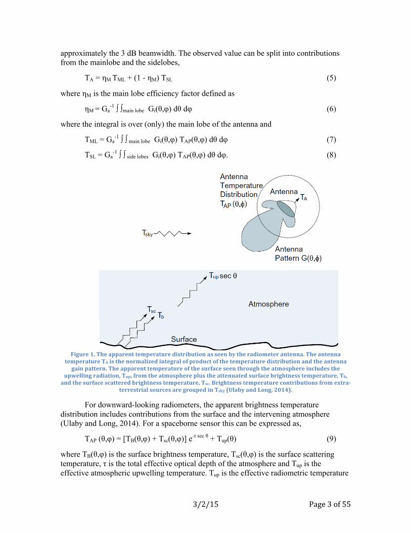
The effective antenna temperature, TA, can be modeled as a product of the apparent temperature distribution TAP(θ,φ) in the look direction θ,φ (see Fig. 1) and the antenna radiation gain F(θ,φ) which is proportional to the antenna gain pattern G(θ,φ) (Ulaby and Long, 2014). TA (in K) is obtained by integrating the product of apparent temperature distribution TAP (θ,φ) (in K) and the antenna pattern G(θ,φ):
TA = Ga-1 ∫ ∫ Gi(θ,φ) TAP(θ,φ) dθ dφ (3)
where
Ga = ∫ ∫ Gi(θ,φ) dθ dφ (4)
Gi(θ,φ) is the instantaneous antenna gain for the particular channel and where the integrals are over the range of values corresponding to the non-negligible gain of the antenna. Note that the antenna pattern acts as a low pass spatial filter of the surface brightness distribution, limiting the primary surface contribution to the observed TB to
3/2/15 Page 3 of 55
approximately the 3 dB beamwidth. The observed value can be split into contributions from the mainlobe and the sidelobes,
TA = ηM TML + (1 - ηM) TSL (5)
where ηM is the main lobe efficiency factor defined as
ηM = Ga-1 ∫ ∫main lobe Gi(θ,φ) dθ dφ (6)
where the integral is over (only) the main lobe of the antenna and
TML = Ga-1 ∫ ∫ main lobe Gi(θ,φ) TAP(θ,φ) dθ dφ (7)
TSL = Ga-1 ∫ ∫ side lobes Gi(θ,φ) TAP(θ,φ) dθ dφ. (8)
Figure 1. The apparent temperature distribution as seen by the radiometer antenna. The antenna temperature TA is the normalized integral of product of the temperature distribution and the antenna gain pattern. The apparent temperature of the surface seen through the atmosphere includes the
upwelling radiation, Tup, from the atmosphere plus the attenuated surface brightness temperature, Tb, and the surface scattered brightness temperature, Tsc. Brightness temperature contributions from extra-
terrestrial sources are grouped in Tsky (Ulaby and Long, 2014).
For downward-looking radiometers, the apparent brightness temperature distribution includes contributions from the surface and the intervening atmosphere (Ulaby and Long, 2014). For a spaceborne sensor this can be expressed as,
TAP (θ,φ) = [TB(θ,φ) + Tsc(θ,φ)] e-τ sec θ + Tup(θ) (9)
where TB(θ,φ) is the surface brightness temperature, Tsc(θ,φ) is the surface scattering temperature, τ is the total effective optical depth of the atmosphere and Tup is the effective atmospheric upwelling temperature. Tup is the effective radiometric temperature
3/2/15 Page 4 of 55
of the atmosphere, which depends on the temperature and density profile, atmospheric losses, clouds, rain, etc.
Ignoring incidence and azimuth angle dependence, the surface brightness temperature is,
TB = ϵTP (10)
where ϵ is the emissivity of the surface and TP is the physical temperature of the surface. The emissivity is a function of the surface roughness and the permittivity of the surface, which are related to the geophysical properties of the surface (Ulaby and Long, 2014). In geophysical studies, the key parameter of interest is ϵ or TB.
The surface scattering temperature, Tsc(θ,φ), is the result of downwelling atmospheric emissions which are scattered off of the rough surface toward the sensor. This signal depends on the scattering properties of the surface (surface roughness and dielectric constant) as well as the atmospheric emissions directed toward the ground. Note that azimuth variation with brightness temperature has been observed over the ocean (Wentz, 1992), sand dunes (Stephen and Long, 2005), and snow in Antarctica (Long and Drinkwater, 2000). Vegetated and sea ice-covered areas generally have little or no azimuth brightness variation.
2.2 Signal Integration The received signal power is very noisy. To reduce the measurement variance,
the received signal power is averaged over a short “integration period.” Even so, the reported measurements are noisy due to the limited integration time available for each measurement. The uncertainty is expressed as ΔT, which is the standard deviation of the temperature measurement. ΔT is a function of the integration time and bandwidth used to make the radiometric measurement and is typically inversely related to the time-bandwidth product (Ulaby and Long, 2014). Increasing the integration time and/or bandwidth reduces ΔT. High stability and precise calibration of the system gain is required to accurately infer the brightness temperature TB from the sensor power measurement PSYS.
Because the antenna is scanning during the integration period, the effective antenna gain pattern of the measurements is a smeared version of the antenna pattern. In the smeared case, we replace Gi in Eqs. 3 & 4 with the “smeared” version of the antenna, Gs where
Gs(θ, φ) = Ti-1 ∫ Gi(θ, φ + Δφ t) dt (11)
where Ti is the integration period, Δφ is the rotation rate, and the integral limits are -Ti and 0. Note that because Ti is very short, the net effect is primarily to widen the main lobe. Nulls in the pattern tend to be eliminated and the sidelobes widened.
Because the antenna pattern has been specifically designed to minimize the power from directions not from the surface, we can neglect the antenna smearing from non-surface contributions and concentrate on the pattern smearing at the surface. The

3/2/15 Page 5 of 55
smeared antenna pattern Gs(θ, φ) projected on the surface at a particular time defines the “measurement spatial response function” (SRF) of the corresponding TB measurement.
Note from Eq. 9 that TAP(θ,φ) consists primarily of an attenuated contribution from the surface (i.e., TB) plus scattered and upwelling terms. We note that the reported TA values compensate or correct (to some degree) for these terms.
Let TA’ denote the corrected TA measurement. It follows that we can re-write Eq. 9 in terms of the corrected TA and the surface TB value as
TA’ = Ga-1 ∫ ∫ Gs(θ,φ) TB(θ,φ) dθ dφ. (12)
We can express this result in terms of the surface coordinates x and y as (noting that for a given x,y location and time, the antenna elevation and azimuth angles can be computed)
TA’ = Gb-1 ∫ ∫ Gs(x,y) TB(x,y) dx dy (13)
where
Gb = ∫ ∫ Gs(x,y) dx dy. (14)
We define the SRF to be
SRF(x,y) = Gb-1 Gs(x,y). (15)
So that,
TA’ = ∫ ∫ SRF(x,y) TB(x,y) dx dy. (16)
Thus, the measurements TA’ can be seen to be the integral of the product of the SRF and the surface brightness temperature and the SRF is a function of the antenna pattern, the observation geometry, and the integration period.
3 Antenna Pattern Accuracy and the SRF The previous section shows that each measurement is the SRF-weighted average
of TB and that the antenna pattern and signal integration coupled with the geometry determine the SRF. In principle very precise knowledge of the antenna pattern is required to properly calibrate the TB measurements. Since high precision antenna pattern measurement is notoriously difficult, uncertainty in the antenna pattern can be quite large compared to the desired measurement. We note, however, that in calibrating the estimated TB values, only the integrated factors such as TML, TSL, and ηM (among others) are needed. Fortunately, these can be determined more precisely post launch through careful data analysis than they can be computed from pre-launch antenna calibration measurements. Thus, knowledge of the precise antenna pattern is not essential for system TB calibration. The antenna pattern calibration measurements primarily serve as a way of predicting performance and computing first guess parameter values that are later refined
3/2/15 Page 6 of 55
during the post-launch period. Determining the SRF, however, does require knowledge of the antenna pattern.
This raises a number of questions: for example, how accurately do we need to know the antenna pattern? And, since the computation can be complicated, can sufficiently accurate, simplified models for the effective SRF be developed?
3.1 Pattern Accuracy Fundamental to answering these questions is the question, how accurately does
the SRF need to be known? The study by Long and Brodzik (2015) broadly considered this question for the CETB. They found that since full reconstruction was not needed for CETB data production, significant errors in the SRF could be tolerated so long as its 3dB size was approximately correct. This is a fortunate result since the antenna patterns for a number of important satellite radiometers (e.g., SMMR) are not known precisely. Further, even for sensors for which antenna patterns are available there is some uncertainty in the orientation of the ground-measured patterns and the on-orbit orientation. In the case of SSMIS the antenna pattern measurements are made at the same angular spacing for all frequencies. This is ideal for the low frequency channels but the available antenna pattern data is too coarse to properly resolve the sidelobes of the 90 GHz channels (see later results). We also note that antenna gain patterns vary with frequency, even within a single channel. In such a case the effective antenna pattern is the average of the patterns at each frequency used, which requires averaging of the measured patterns.
With these considerations in mind, we conclude that we need only estimate the effective antenna pattern to a reasonable level of accuracy that includes accurately describing the main lobe size, i.e. over the main lobe the model should be better than order 1 dB over the 3dB mainlobe. In the remainder of this section we consider the antenna pattern. The full SRF is addressed later.
For approximating the antenna pattern we desire a simple, yet robust model that can be easily applied in all cases. A Gaussian function is a particularly simple and commonly used model that, as shown below, fits the main lobe well. To fit the sidelobes, adding a second, flatter Gaussian improves the fit (see Appendix B). However, this is not needed in our application, i.e. the side lobe performance can be ignored due to the very small contribution of the signal in the sidelobes resulting from the low gain there.
In the following we show that a simple Gaussian approximation based on the 3dB footprint can be used to accurately model the mainlobe of the antenna gain pattern. Extending the model to a so-called dual-Gaussian model improves the model to include the sidelobes. We first consider idealized patterns for the SSM/I, then actual measured patterns for SSMIS.
3.2 Approximate SSM/I Antenna Pattern Modeling
Lacking a measured SSM/I antenna pattern, we use an approximate model based on a particular assumed aperture function discussed in Appendix C. The following is
3/2/15 Page 7 of 55
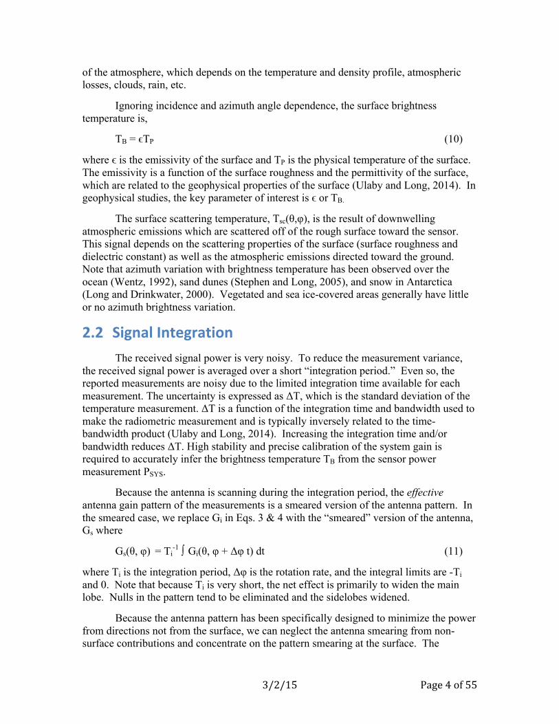
based on using this antenna pattern. The results for using an alternate pattern are provided in Appendix C. In this section, we consider antenna gain patterns using a squared sine-squared antenna pattern, which is similar to those commonly used in microwave antennas. We consider the effects of scanning and integration on the effective pattern and the accuracy of a Gaussian fit to the gain pattern for the 19, 37, and 85 GHz SSM/I channels. Figure 2 illustrates the geometry of a typical measurement. The effective footprint size is the projection of the 3dB integrated antenna response on to the surface.
To compute the effective antenna pattern after integration, the geometry illustrated in Fig. 2 is used. Knowing the antenna rotation rate, the incidence angle, and platform altitude (see the Appendix), the azimuth angle range that corresponds to the temporal integration window can be computed. The integrated pattern is then computed by summing shifted azimuth gain patterns. The resulting integrated pattern is then normalized to a unity peak gain.
Figure 2. Radiometer measurement geometry. The yellow box illustrates the “box-car” 3dB pattern
approximation at the surface.
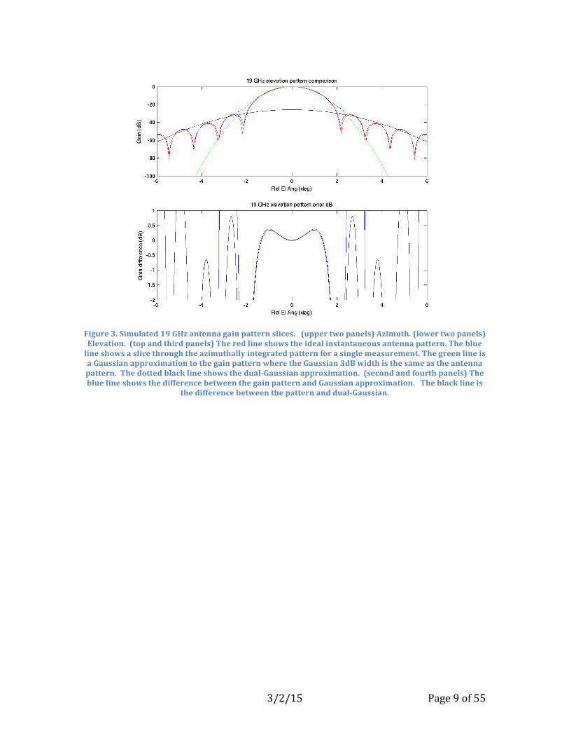
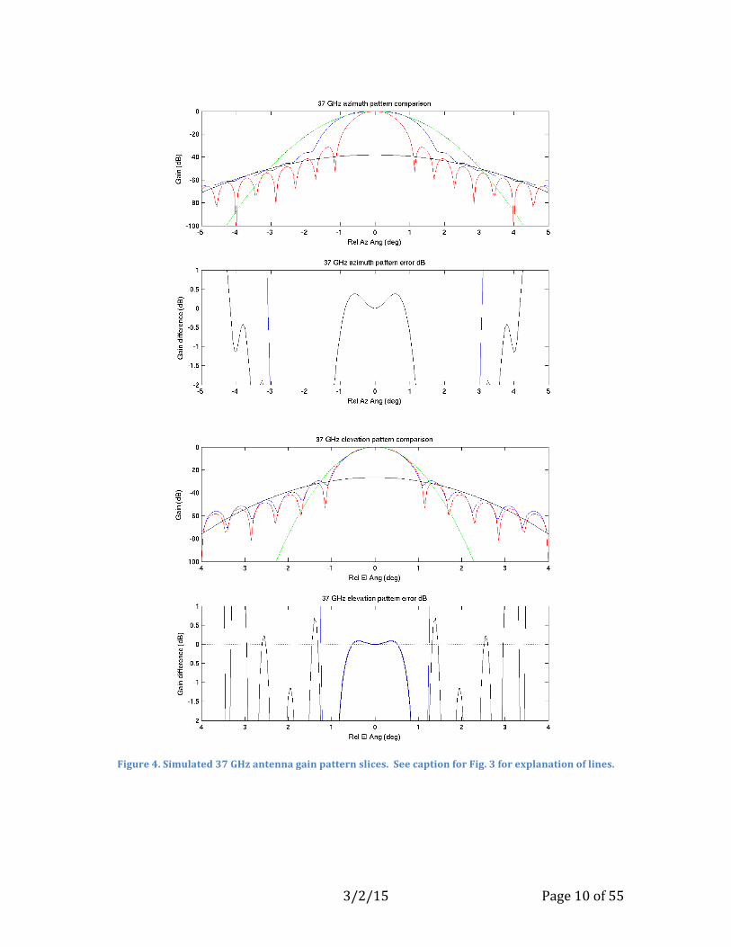
Figure 3 shows the azimuth and elevation patterns for the 19 GHz channel, while Figs. 4 and 5 similarly show the patterns for 37 and 85 GHz channels. These are intended to be representative, but do not need to be exact to illustrate the points considered. Note that the effects of the integration on the antenna pattern in the azimuth direction vary with channel, but tend to eliminate the pattern nulls. The integration does not affect the elevation pattern very much. The Gaussian fit models the main lobe fairly well (within a few tenths of a dB), but it does not include the sidelobes. The dual-Gaussian model (described in Appendix B) fits the pattern envelope quite well at low frequencies, except in the areas of the nulls which have low gain and thus do not contribute much to the measured brightness temperature. Both Gaussian fits are less

3/2/15 Page 8 of 55
accurate at high frequencies, but still accurately describe the mainlobe 3dB width. Given the relative insensitivity of the reconstruction to the details of the pattern roll off below -10 dB, the single Gaussian is subjectively judged to be adequate for this project.
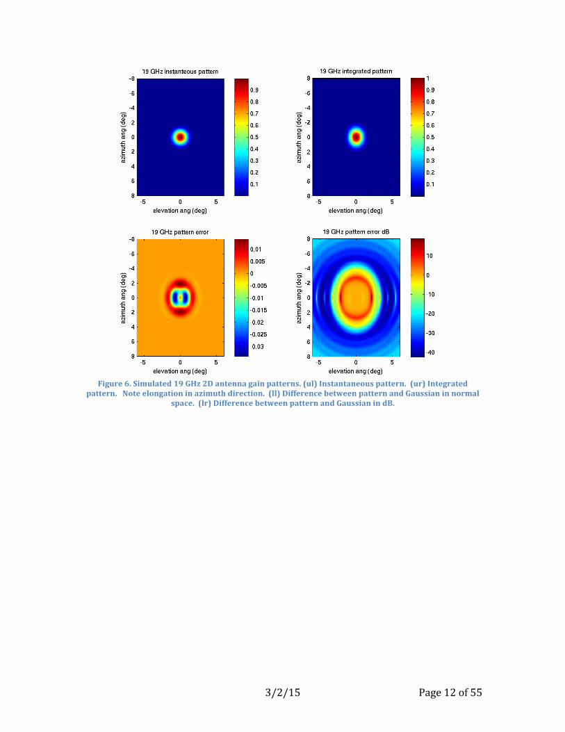
The 3D patterns showing the same effects are illustrated in Figs. 6-8. Again, it apparent that a Gaussian does well for modeling the main lobe but not the side lobes. Though not shown here, using a dual-Gaussian works well in the 2D case, too.
3/2/15 Page 9 of 55
Figure 3. Simulated 19 GHz antenna gain pattern slices. (upper two panels) Azimuth. (lower two panels) Elevation. (top and third panels) The red line shows the ideal instantaneous antenna pattern. The blue line shows a slice through the azimuthally integrated pattern for a single measurement. The green line is a Gaussian approximation to the gain pattern where the Gaussian 3dB width is the same as the antenna pattern. The dotted black line shows the dual-Gaussian approximation. (second and fourth panels) The blue line shows the difference between the gain pattern and Gaussian approximation. The black line is
the difference between the pattern and dual-Gaussian.
3/2/15 Page 10 of 55
Figure 4. Simulated 37 GHz antenna gain pattern slices. See caption for Fig. 3 for explanation of lines.

3/2/15 Page 11 of 55
Figure 5. Simulated 37 GHz antenna gain pattern slices. See caption for Fig. 3 for explanation of lines.
3/2/15 Page 12 of 55
Figure 6. Simulated 19 GHz 2D antenna gain patterns. (ul) Instantaneous pattern. (ur) Integrated
pattern. Note elongation in azimuth direction. (ll) Difference between pattern and Gaussian in normal space. (lr) Difference between pattern and Gaussian in dB.

3/2/15 Page 13 of 55
Figure 7. Simulated 37 GHz 2D antenna gain patterns. (ul) Instantaneous pattern. (ur) Integrated
pattern. Note elongation in azimuth direction. (ll) Difference between pattern and Gaussian in normal space. (lr) Difference between pattern and Gaussian in dB.

3/2/15 Page 14 of 55
Figure 8. Simulated 85 GHz 2D antenna gain patterns. (ul) Instantaneous pattern. (ur) Integrated
pattern. Note elongation in azimuth direction. (ll) Difference between pattern and Gaussian in normal space. (lr) Difference between pattern and Gaussian in dB.
3.3 SSMIS Antenna Patterns
For the SSMIS, detailed antenna pattern measurements are available from the Aerospace Corporation for for each of the flight antennas (Donald Boucher, personal communication). In this section, we use the measured patterns to repeat the analysis previously shown for simulated SSM/I measurements. Two-D patterns were measured at each of several frequencies within the bandwidth of each channel. However, noting their similarity within a band, the uncertainty in knowing precisely how the patterns are oriented for a particular sensor, we use a single frequency near the band center. The original patterns are measured at 1 deg increments. For calculating the integrated patterns, they are first interpolated to 0.1 deg increments. The resulting slices patterns are shown in Figs. 9-11. A two-D pattern was created by interpolating in azimuth angle at each fixed elevation using the four available azimuth slices. The results are illustrated in Figs. 12-14. Only a single polarization at each channel frequency is considered.

3/2/15 Page 15 of 55
Each plot consists of 4 elevation angle slices at different azimuth angles, 0, 45, 90, and 135. (Slices at 180, 225, 270, and 315 are redundant.) It is not certain how the flight antenna azimuth angle is aligned with the calibration azimuth angle. A Gaussian fit to the main lobe is shown for the 0 and 90 deg azimuth slices. These reasonably well approximate the shape of the main lobe. Note the while the 19 GHz channel has well defined sidelobes, the sidelobes for the other channel are less well defined and that the coarse measurement resolution for the 90 GHz channel results in poorly defined sidelobes. Similarly, for the 2D case, the Gaussian model does a good job of describing the mainlobe, though it does not fit the sidelobes.
Figure 9. SSMIS measured 19 GHz antenna gain pattern slices.

3/2/15 Page 16 of 55
Figure 10. SSMIS measured 37 GHz antenna gain pattern slices.
Figure 11. SSMIS measured 90 GHz antenna gain pattern slices.

3/2/15 Page 17 of 55
Figure 12. SSMI measured 19 GHz 2D antenna gain patterns. (ul) Instantaneous pattern. (ur) Integrated pattern. Note smearing of sidelobe nulls. (ll) Difference between pattern and Gaussian in normal space.
(lr) Difference between pattern and Gaussian in dB.
Figure 13. SSMI measured 37 GHz 2D antenna gain patterns. (ul) Instantaneous pattern. (ur) Integrated pattern. Note smearing of sidelobe nulls. (ll) Difference between pattern and Gaussian in normal space.
(lr) Difference between pattern and Gaussian in dB.

3/2/15 Page 18 of 55
Figure 14. SSMI measured 37 GHz 2D antenna gain patterns. (ul) Instantaneous pattern. (ur) Integrated pattern. Note smearing of sidelobe nulls. (ll) Difference between pattern and Gaussian in normal space.
(lr) Difference between pattern and Gaussian in dB.
4 Antenna Pattern to SRF Transformation The previous section considered modeling the antenna pattern. Here the SRF is
considered. Recall from Eqs. 14 and 15 that the SRF is the projection of the integrated antenna pattern on the Earth’s surface, see Fig. 2. Computing the SRF from the antenna pattern requires transforming the antenna pattern expressed in azimuth and elevation angles into gain at the surface expressed in horizontal displacement from the location of the antenna boresite on the Earth’s surface.
A brief philosophical comment regarding accuracy: When there is a lot of uncertainty in the inputs, it may not make sense to model the system too precisely (i.e., use overly complicated computational models) since errors in the system output will be dominated by errors or noise in the input rather than by model approximations. Of course, one must verify that the modelling approximations do not introduce significant errors.
With this in mind, we note that it is possible to use essentially exact computations in transforming from antenna az/el coordinates to ground position coordinates. However, significantly more information about the orbit, scan angle, spacecraft attitude, etc. are required by such a model. Instead, we use a number of simplifying assumptions that provide adequate accuracy and permit better insight into the computation. These are summarized below.
3/2/15 Page 19 of 55
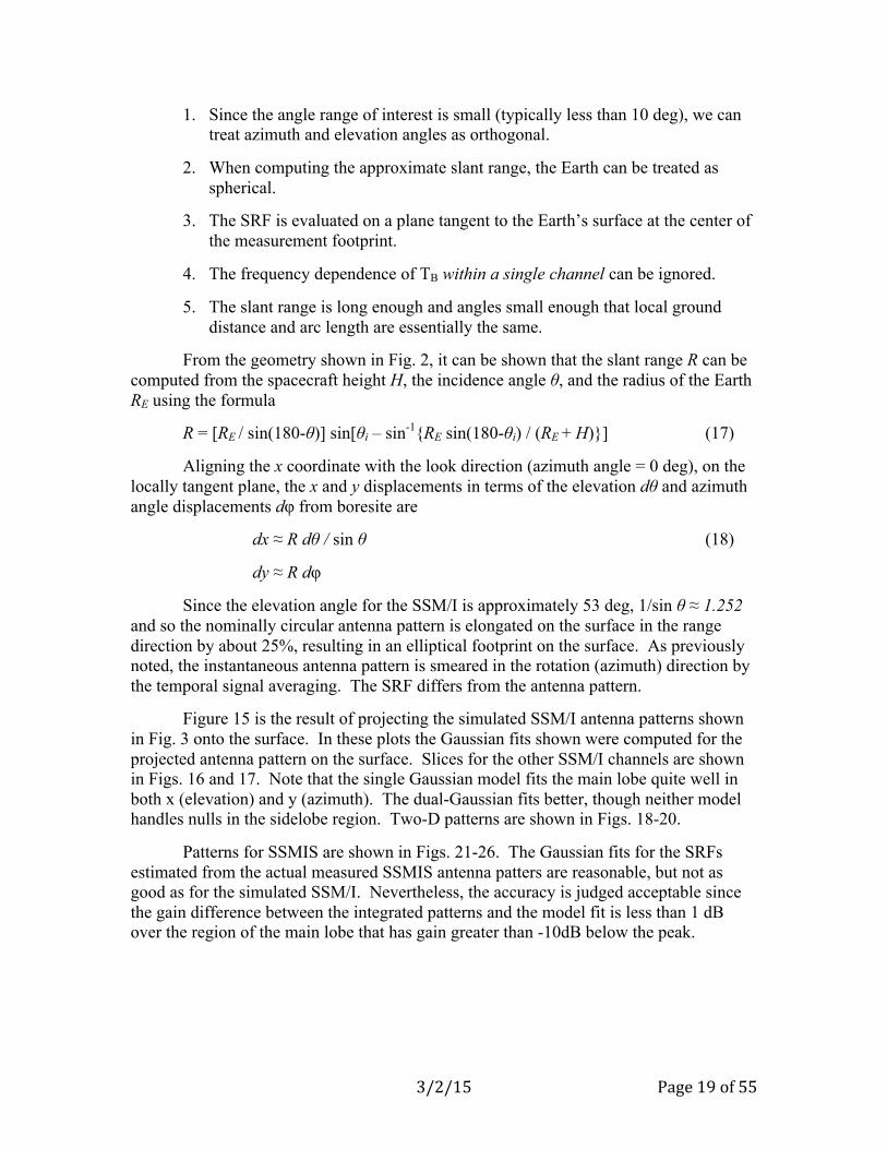
1. Since the angle range of interest is small (typically less than 10 deg), we can treat azimuth and elevation angles as orthogonal.
2. When computing the approximate slant range, the Earth can be treated as spherical.
3. The SRF is evaluated on a plane tangent to the Earth’s surface at the center of the measurement footprint.
4. The frequency dependence of TB within a single channel can be ignored.
5. The slant range is long enough and angles small enough that local ground distance and arc length are essentially the same.
From the geometry shown in Fig. 2, it can be shown that the slant range R can be computed from the spacecraft height H, the incidence angle θ, and the radius of the Earth RE using the formula
R = [RE / sin(180-θ)] sin[θi – sin-1{RE sin(180-θi) / (RE + H)}] (17)
Aligning the x coordinate with the look direction (azimuth angle = 0 deg), on the locally tangent plane, the x and y displacements in terms of the elevation dθ and azimuth angle displacements dφ from boresite are
dx ≈ R dθ / sin θ (18)
dy ≈ R dφ
Since the elevation angle for the SSM/I is approximately 53 deg, 1/sin θ ≈ 1.252 and so the nominally circular antenna pattern is elongated on the surface in the range direction by about 25%, resulting in an elliptical footprint on the surface. As previously noted, the instantaneous antenna pattern is smeared in the rotation (azimuth) direction by the temporal signal averaging. The SRF differs from the antenna pattern.
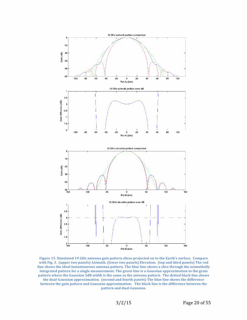
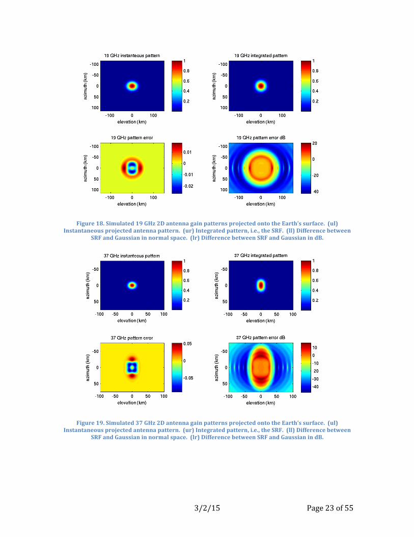
Figure 15 is the result of projecting the simulated SSM/I antenna patterns shown in Fig. 3 onto the surface. In these plots the Gaussian fits shown were computed for the projected antenna pattern on the surface. Slices for the other SSM/I channels are shown in Figs. 16 and 17. Note that the single Gaussian model fits the main lobe quite well in both x (elevation) and y (azimuth). The dual-Gaussian fits better, though neither model handles nulls in the sidelobe region. Two-D patterns are shown in Figs. 18-20.
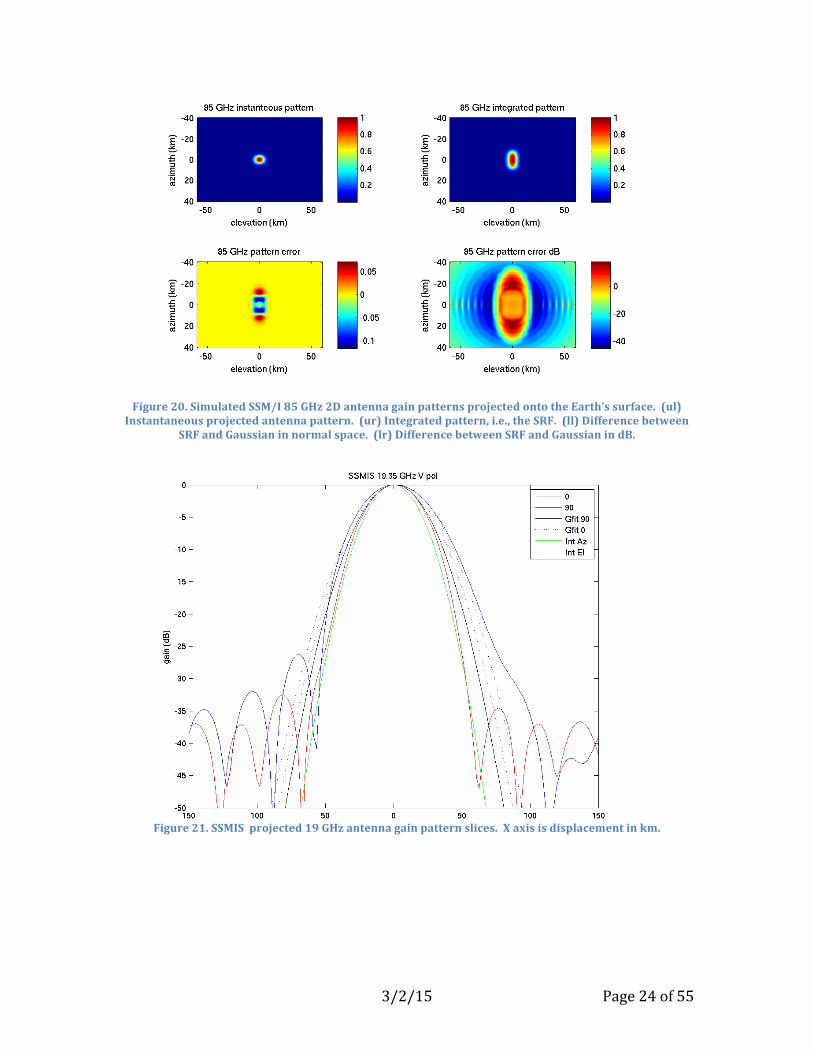
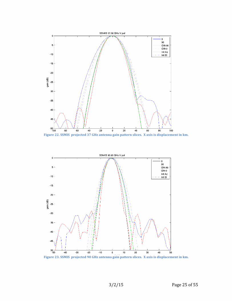
Patterns for SSMIS are shown in Figs. 21-26. The Gaussian fits for the SRFs estimated from the actual measured SSMIS antenna patters are reasonable, but not as good as for the simulated SSM/I. Nevertheless, the accuracy is judged acceptable since the gain difference between the integrated patterns and the model fit is less than 1 dB over the region of the main lobe that has gain greater than -10dB below the peak.
3/2/15 Page 20 of 55
Figure 15. Simulated 19 GHz antenna gain pattern slices projected on to the Earth’s surface. Compare with Fig. 3. (upper two panels) Azimuth. (lower two panels) Elevation. (top and third panels) The red line shows the ideal instantaneous antenna pattern. The blue line shows a slice through the azimuthally integrated pattern for a single measurement. The green line is a Gaussian approximation to the grain pattern where the Gaussian 3dB width is the same as the antenna pattern. The dotted black line shows
the dual-Gaussian approximation. (second and fourth panels) The blue line shows the difference between the gain pattern and Gaussian approximation. The black line is the difference between the
pattern and dual-Gaussian.

3/2/15 Page 21 of 55
Figure 16. Simulated 37 GHz antenna gain pattern slices projected on to the Earth’s surface. See caption
for Fig. 15.

3/2/15 Page 22 of 55
Figure 17. Simulated 85 GHz antenna gain pattern slices projected on to the Earth’s surface. See caption
for Fig. 15.
3/2/15 Page 23 of 55
Figure 18. Simulated 19 GHz 2D antenna gain patterns projected onto the Earth’s surface. (ul) Instantaneous projected antenna pattern. (ur) Integrated pattern, i.e., the SRF. (ll) Difference between
SRF and Gaussian in normal space. (lr) Difference between SRF and Gaussian in dB.
Figure 19. Simulated 37 GHz 2D antenna gain patterns projected onto the Earth’s surface. (ul) Instantaneous projected antenna pattern. (ur) Integrated pattern, i.e., the SRF. (ll) Difference between
SRF and Gaussian in normal space. (lr) Difference between SRF and Gaussian in dB.
3/2/15 Page 24 of 55
Figure 20. Simulated SSM/I 85 GHz 2D antenna gain patterns projected onto the Earth’s surface. (ul) Instantaneous projected antenna pattern. (ur) Integrated pattern, i.e., the SRF. (ll) Difference between
SRF and Gaussian in normal space. (lr) Difference between SRF and Gaussian in dB.
Figure 21. SSMIS projected 19 GHz antenna gain pattern slices. X axis is displacement in km.
3/2/15 Page 25 of 55
Figure 22. SSMIS projected 37 GHz antenna gain pattern slices. X axis is displacement in km.
Figure 23. SSMIS projected 90 GHz antenna gain pattern slices. X axis is displacement in km.

3/2/15 Page 26 of 55
Figure 24. SSMIS measured 19 GHz 2D antenna gain patterns. (ul) Instantaneous pattern. (ur) Integrated pattern. Note smearing of sidelobe nulls. (ll) Difference between pattern and Gaussian in normal space.
(lr) Difference between pattern and Gaussian in dB.
Figure 25. SSMIS measured 37 GHz 2D antenna gain patterns. See caption Fig. 24.

3/2/15 Page 27 of 55
Figure 26. SSMIS measured 90 GHz 2D antenna gain patterns. See Caption Fig. 25.
5 Antenna Pattern Ground Spectrum In this section the wavenumber spectrum of the SRF and the antenna pattern as
projected on the surface are considered. This provides insight into the spatial frequency content of the TB measurements and hence the resolution enhancement capability.
5.1 Relation of the Antenna Pattern to the Effective Aperture Illumination Function
It is well known that the far-field antenna pattern can be expressed as the Fourier transform of the electric field across the effective aperture of the antenna (Ulaby and Long, 2014). Since the latter is, by definition, finite extent, this implies that the antenna pattern is bandlimited, i.e., there is an upper limit to the wavenumber spectral content of the antenna pattern. This argument has been use to suggest that the wavenumber spectrum (the two dimensional spatial Fourier transform) of the SRF is also bandlimited. However, it should be noted that the aperture-to-far-field Fourier transform is computed in angular units, while the spectrum of the SRF is computed in distance on the surface. There is a non-linear transformation between angle and surface distance. Further, the angular Fourier transform is computed over a sphere and is periodic in angle whereas the surface spectrum Fourier is computed over a finite domain and is therefore infinite in extent. In the following we consider these issues in more detail and compute the spectrum of the SRF.

3/2/15 Page 28 of 55
Figure 27. (top) Geometry of circular aperture. (bottom) Antenna pattern assuming constant illumination, i.e. Ea=constant over the aperture, zero elsewhere. (Ulaby and Long, 2014)
For simplicity, we consider a circularly symmetric antenna, though similar results can be derived for a general antenna aperture and antenna pattern. Figure 27 illustrates the antenna aperture and resulting radiation pattern. Kirchoff’s scalar diffraction theory shows that the radiated far-field electric field E(R,θ,φ) is related to the electric field across the aperture by the general expressions (Ulaby and Long, 2014)
€
E(R,θ,ϕ) =jλe− jkR
R⎛
⎝ ⎜
⎞
⎠ ⎟ h(θ,ϕ)
h(θ,ϕ) = Ea (xa,ya )exp[ jk sinθ (∫∫ xa cosϕ + ya sinϕ)]dxadya
(19)
where j=√-1, k=2π/λ where λ is the microwave wavelength, and the double integral is computed over the region for which aperture illumination function Ea is non-zero – a finite region that is the effective antenna aperture. The exponential factor in parenthesis is the spherical propagation factor.
For a circular aperture with circularly symmetric aperture illumination, a rectangular to polar transformation is used with

3/2/15 Page 29 of 55
€
xa = ra cosφaya = ra sinφa
(20)
then,
€
h(θ,ϕ) = Ea (ra )exp[ jkra sinθ(cosφa cosϕ + sinφa sinϕ)]dradφa0
a
∫0
2π
∫
h(θ,ϕ) = Ea (ra )exp[ jkra sinθ cos(φa −ϕ)]dradφa0
a
∫0
2π
∫
h(θ,ϕ) = h(θ) = 2π Ea (ra )J0(kra sinθ )dradφa0
2π
∫
(21)
where J0(k) is a zeroth order Bessel function of the first kind,
€
J0(k) = exp[ jkx cos(φa −ϕ)]dφa0
2π
∫ (22)
The far-field antenna pattern F(θ,φ) is then F(θ,φ)=|E(R,θ,φ)R|2/2η0 where η0 is the impedance of free space (Ulaby and Long, 2014).
The resulting antenna pattern for the case where Ea=constant is shown in Fig. 27. In general, however, the illumination function is tapered or windowed. This reduces the sidelobes and the expense of a wider mainlobe, but does not change the region of support of the antenna, i.e. the true “bandwidth” of the pattern remains the same, though parts of it are attenuated differently. The simulated SSM/I pattern previously considered in this report uses a cosine-squared (also sometime termed a sine-squared) taper function.
5.2 Relationship of the SRF Wavenumber Spectrum to the Antenna Illumination Function
As previously discussed, the SRF results from projecting the antenna pattern onto the surface (see Fig. 2) and integrating the moving pattern over the integration period. The resulting gain pattern on the surface is a non-linearly stretched and smeared version of the antenna pattern. Note that due to the curvature of the earth, not all of the antenna pattern will be projected onto the Earth’s surface. Thus the SRF contains only part of the antenna pattern, i.e. the pattern is “clipped”. The clipping introduces a rectangular window or boxcar function into the transformation between antenna pattern and SRF, though where the response function has low gain.
We are interested in the wavenumber (i.e., the spatial) spectrum of the SRF, which is the Fourier transform (in x,y on the surface) of the SRF. This is related to the aperture illumination function, but the transformation is non-linear due to the non-linear, clipped projection. This non-linearity can produce a broader region of support for the SRF wavenumber spectrum than suggested by the finite region of support of the antenna pattern illumination function.

3/2/15 Page 30 of 55
In principle we can analytically compute the wavenumber (spatial) spectrum of the SRF from the projecting and clipping function. However, this is quite complicated. To provide insight into the nature of the various spectra, we first use a simplified representation of the problem.
Referring to the geometry illustrated in Fig. 2 and the pattern illustrated in Fig. 27, the antenna pattern is a sinc2-like function in the variable sin θ where θ is the elevation angle. Using the simplified projection expressions in Eqs. 17 and 18 (note that there is some potential notational confusion since θ is also used for both elevation angle and the local incidence angle – a standard convention in both cases), the antenna pattern on the surface as a function of ground distance is a non-linearly “stretched” copy of the pattern due to the oblique viewing angle. Note that locally the curvature of the Earth was earlier ignored. However, as the distance from the intersection of the boresite vector and Earth’s surface increases, the tangent plane approximation is less appropriate, and it can be seen that only part of the antenna pattern intersects the surface. Thus the projected antenna gain pattern on the Earth’s surface is a clipped version of the antenna pattern. This can be modeled as the multiplication of the stretched antenna pattern by a rectangular window or boxcar function. (Technically, since the antenna pattern is proportional to the magnitude of the electric field at a fixed radius from the antenna, but the projection distance changes as a function of angle, the clipping window should include a taper function based on varying distance from the antenna and the Earth’s surface. For simplicity, this is ignored in the following discussion and in the numerical results presented later. The taper does not affect the region of support, only the magnitude of the spectrum.)
The projected antenna pattern on the surface is thus a non-linearly stretched and windowed version of the original pattern. Recall from signal processing theory that the Fourier transform of the product of two functions is the convolution of the Fourier transforms of the individual functions. In this case, the convolution will yield a wider region of support in frequency domain than either of the individual functions has. Further since the window function is finite length, its Fourier transform is infinite in extent (though it can have nulls). The convolution of an infinite function with any function results in an infinite function. It thus becomes apparent that the region of support of the SRF is not bounded, i.e., it is not bandlimited, even though the aperture illumination pattern is. However, the high wavenumber portion of the spectrum may unrecoverable due to low gain, and there may be nulls in the wavenumber spectrum.
Figure 28 illustrates a slice through the simulated 19 GHz SSM/I pattern over the full angular extent of the pattern (the effects of spacecraft blockage are ignored). The corresponding Fourier transform is also shown. Due to the approximation used in computing the far-field pattern, the spectrum is not perfect, but exhibits high frequency information. Other channels have similar results, though for shorter wavelengths the pattern is narrower and the frequency support wider.

3/2/15 Page 31 of 55
Figure 28. (top) Magnitude squared plot of slice through the simulated 19 GHz SSM/I channel antenna pattern. (bottom) Magnitude Fourier transform. This is the magnitude of the aperture illumination function. Note that the region of support is (effectively) limited to low frequencies due to the finite
extent of the aperture illumination function.
To compute the spectrum of the antenna pattern projected onto the Earth’s surface along the elevation axis we again use the geometry shown in Fig. 2. Additional variables are introduced in Fig. 29. To enable computation on a larger area, rather than use a tangent plane approximation, the arc length on the surface is used here.

3/2/15 Page 32 of 55
Figure 29. Geometry for arc-length computation.
Given the elevation angle and height, for a particular displacement Δx the Earth angles α and α0 can be computed using
ξ = sin-1[(Re/(Re+H)) sin (180-θ)] (23)
α = θ - ξ
α0 = α - Δx / Re
The antenna elevation angle Δθ corresponding to the point of interest is computed as
R0 = sqrt[(Re+H)2 + Re2-2(Re+H)Re cos α0] (24)
ξ0 = sin-1[(Re/R0) sin α0]
Δθ = ξ - ξ0
Computation of the azimuth angle is more complicated and not treated here.
Figures 30-32 illustrate the magnitude Fourier transform of elevation slices of the antenna pattern projected on to the Earth’s surface. Note that the spatial spectrum is in wavenumber space which has units of inverse ground distance and that the region of support extends to a broader range of spatial frequencies, i.e. the rolloff is slower. This suggests we can recover more spatial information. Based on experience, in practice we can only hope to recover information when the gain is higher than -10 dB, or perhaps -20 dB in the best case. Table 1 summarizes the cutoff points for all the channels at different gain thresholds.

3/2/15 Page 33 of 55
Table 1. Cutoff scales in km for simulated SSM/I channels.
Channel Spatial Scale (in km) at gain cutoff Frequency -20 dB -10 dB -3 dB
19 27.3 36.5 63.8 37 14.4 19.1 33.3 85 6.3 8.3 14.5
Figure 30. (top) Antenna pattern for the simulated 19 GHz SSM/I channel projected on to the Earth surface versus (arc length) displacement along the surface. The x axis is the range over which the platform is visible from the surface. Note the variable spacing of the sidelobes. . Compare to Fig. 3.
(bottom) Magnitude Fourier transform of slice of the projected antenna pattern. The vertical line is at --20 dB and corresponds to a 27 km spatial scale.

3/2/15 Page 34 of 55
Figure 31. (top) Antenna pattern for the simulated 37 GHz SSM/I channel projected on to the Earth surface versus (arc length) displacement along the surface. The x axis is the range over which the platform is visible from the surface. Note the variable spacing of the sidelobes. . Compare to Fig. 3.
(bottom) Magnitude Fourier transform of slice of the projected antenna pattern. The vertical line is at --20 dB and corresponds to a 14.4 km spatial scale.
We note that since these results are based on approximate (i.e., simulated) antenna patterns the results look more precise than they probably really are, particularly since the analytic antenna pattern assumed rolls off faster than the realistic. Nevertheless we can observe that using the -10 dB cutoff, the 25 km sample spacing provided by the instrument oversamples the 19 GHz channels, but is about the right value for the 37 GHz channels. The 85 GHz channels are sampled at 12.5 km, and so they are slightly undersampled. Note, however that to achieve effective recovery of the frequency content down to -10 dB (or more), some sort of reconstruction processing is required. Classic drop in the bucket resolution is limited to approximately the 3 dB resolution, which this table suggests is much coarser than the sampling.
3/2/15 Page 35 of 55
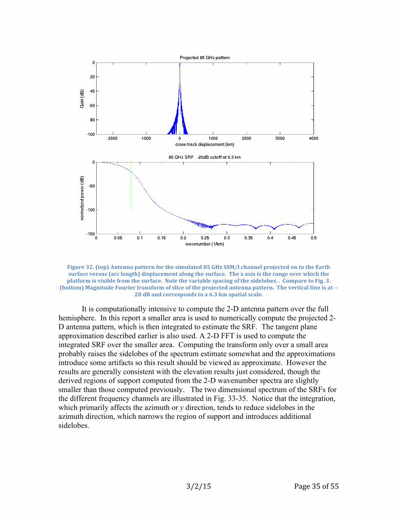
Figure 32. (top) Antenna pattern for the simulated 85 GHz SSM/I channel projected on to the Earth surface versus (arc length) displacement along the surface. The x axis is the range over which the platform is visible from the surface. Note the variable spacing of the sidelobes. . Compare to Fig. 3.
(bottom) Magnitude Fourier transform of slice of the projected antenna pattern. The vertical line is at --20 dB and corresponds to a 6.3 km spatial scale.
It is computationally intensive to compute the 2-D antenna pattern over the full hemisphere. In this report a smaller area is used to numerically compute the projected 2-D antenna pattern, which is then integrated to estimate the SRF. The tangent plane approximation described earlier is also used. A 2-D FFT is used to compute the integrated SRF over the smaller area. Computing the transform only over a small area probably raises the sidelobes of the spectrum estimate somewhat and the approximations introduce some artifacts so this result should be viewed as approximate. However the results are generally consistent with the elevation results just considered, though the derived regions of support computed from the 2-D wavenumber spectra are slightly smaller than those computed previously. The two dimensional spectrum of the SRFs for the different frequency channels are illustrated in Fig. 33-35. Notice that the integration, which primarily affects the azimuth or y direction, tends to reduce sidelobes in the azimuth direction, which narrows the region of support and introduces additional sidelobes.

3/2/15 Page 36 of 55
Figure 33. 2-D antenna patterns (top row) and spectra (bottom row) for the simulated 19 GHz frequency
channels. The instantaneous and integrated patterns are shown. The latter is the SRF.

3/2/15 Page 37 of 55
Figure 34. 2-D antenna patterns (top row) and spectra (bottom row) for the simulated 37 GHz frequency channels. The instantaneous and integrated patterns are shown. The latter is the SRF. Note the nulls
introduced into the frequency response of the SRF due to the azimuth integration.

3/2/15 Page 38 of 55
Figure 35. 2-D antenna patterns (top row) and spectra (bottom row) for the simulated 85 GHz frequency channels. The instantaneous and integrated patterns are shown. The latter is the SRF. Note the nulls
introduced into the frequency response of the SRF due to the azimuth integration.
6 Conclusion For partial reconstruction a precise model of the spatial response function is not
required—all that is required is an accurate representation of the mainlobe. While some measured antenna patterns are available for some sensors, in some cases accurate patterns are not available. Even when available, there is significant uncertainty in applying the measured patterns. Using simplified models for the SRF can enable consistent processing for multiple sensors. A particularly simple model can be achieved by using a 2D Gaussian with 3dB size the same as the integrated antenna pattern on the surface, i.e. to the effective footprint size.
This report has examined the effective frequency response of the SRF and how the antenna pattern, coupled with the measurement geometry, dictates the recoverable spatial information. It is shown that the SRF has recoverable frequency information in excess of its 3dB width.

3/2/15 Page 39 of 55
7 References Brodzik, M. J. and D.G. Long. 2014. “Calibrated Passive Microwave Daily EASE-Grid 2.0 Brightness Temperature ESDR (CETB): Algorithm Theoretical Basis Document,” National Snow and Ice Data Center (NSIDC) publication [Online] Available at: (TBD link needed). Hollinger, J., et al., “Special Sensor Microwave/Imager User's Guide,” Naval Research Laboratory, Washington, D.C., Dec. 14, 1987. Hollinger, J., “DMSP Special Sensor Microwave/Imager Calibration/Validation, Final Report, Volume 1,” Naval Research Laboratory, Washington, D.C., July 1989. Kunkee, D.B., G. A. Poe, D. J. Boucher, S. D. Swadley, Y. Hong, J. E. Wessel, and E. A. Uliana, “Design and Evaluation of the First Special Sensor Microwave Imager/Sounder,” IEEE Transactions on Geoscience and Remote Sensing, Vol. 46, No. 4, pp. 863–883, 2008. Long, D.G., and M.J. Brodzik. 2015. “Calibrated Passive Microwave Daily EASE-Grid 2.0 Brightness Temperature ESDR (CETB): Selection of Gridding Parameters,” National Snow and Ice Data Center (NSIDC) publication [Online] Available at: (TBD link needed). Long, D.G., “Microwave Sensors - Active and Passive,” in M.W. Jackson, R.R. Jensen and S.A. Morain (eds), Manual of Remote Sensing, Volume 1: Earth Observing Platforms and Sensors, 4th Edition, American Society for Photogrammetry and Remote Sensing, Bethesda, Maryland, 2008. Ulaby, F., and D.G. Long, Microwave Radar and Radiometric Remote Sensing, University of Michigan Press, Ann Arbor, Michigan, 2014.

3/2/15 Page 40 of 55
8 Appendix A: Radiometer Sensors
The SSM/I and SSMIS sensors are briefly described in the following sections. More detailed descriptions are provided in the cited literature.
8.1 Special Sensor Microwave/Imager (SSM/I)
The SSM/I is a total-power radiometer with seven operating channels, see Table 1. These channels cover four different frequencies with horizontal and vertical polarizations channels at 19.35, 37.0, and 85.5 GHz and a vertical polarization channel at 22.235 GHz. An integrate-and-dump filter is used to make radiometric brightness temperature measurements as the antenna scans the ground track via antenna rotation (Hollinger, 1989; 1987). As specified by Hollinger et al. (1987) the 3 dB elliptical antenna footprints range from about 15-70 km in the cross-scan direction and 13-43 km in the along-scan direction depending on frequency. First launched in 1987, SSM/I instruments have flown on multiple spacecraft continuously until the present on the Defense Meteorological Satellite Program (DMSP) (F) satellite series. The nominal orbit height is 833 km.
Table 1: SSM/I Channel Characteristics (Hollinger, 1987)
Channel Name
Polarization Center Frequency
(GHz)
Bandwidth (MHz)
3 dB Footprint Size (km)
Integration Period (ms)
Channel ΔT* (K)
19H H 19.35 125 43 × 69 7.95 0.42 19V V 19.35 125 43 × 69 7.95 0.45
22 V 22.23 300 40 × 60 7.95 0.74 37H H 37 750 28 × 37 7.95 0.38 37V V 37 750 20 × 37 7.95 0.37 85H H 85.5 2000 13 × 15 3.89 0.73 85V V 85.5 2000 13 × 15 3.89 0.69
* Estimated instrument noise for the F08 SSM/Is. Actual values vary between sensors.
The SSM/I scanning concept is illustrated in Figure A1. The antenna spin rate is 31.6 rpm with an along-track spacing of approximately 12.5 km. The measurements are collected at a nominal incidence angle of approximately 53°. The scanning geometry produces a swath coverage diagram as shown in Fig. A2. The integrate and dump filter lengths for each channel are shown in the table.

3/2/15 Page 41 of 55
Figure A1. Illustration of the SSM/I scanning concept. The antenna and feed are spun about the vertical axis. Due to the along-track translation of the nadir point resulting from spacecraft motion in its orbit, the resulting scan pattern on the surface is an overlapping helix. Due to interference from the spacecraft
structure, only part of the rotation is useful for measuring the surface TB, see Fig, 2. The rest of the rotation time is used for calibration. The observation incidence angle is essentially constant as the
antenna scans the surface. (Long, 2008)
Figure A2. SSM/I coverage swath. The dark ellipse schematically illustrates the antenna 3dB response mainlobe on the surface for a particular channel at a particular antenna scan angle as illustrated by the light dashed line. The orientation of the ellipse varies relative to the ground track due to the rotation of the antenna, which is centered at the top of the diagram. The observation swath is defined the rotation of the antenna through a total scan angle range of 102°. The dark dashed line represents the spacecraft nadir ground track. The measurement incidence angle remains essentially constant during the scan. This diagram is for the aft-looking F08 SSM/I. Later SSM/Is looked forward, but had same swath width.
!

3/2/15 Page 42 of 55
8.2 Special Sensor Microwave Imager/Sounder (SSMIS)
The Special Sensor Microwave Imager/Sounder (SSMIS) is a total-power radiometer with 24 operating channels, see Table A2 (Kunkee, 2008). The antenna rotation rate is 31.6 rpm with measurements collected at a nominal incidence angle of 53.1° producing a nominal swath width of 1700 km and an along-track spacing of nominal 12.5 km. First launched in 2003, SSMIS instruments have flown on multiple spacecraft (F-17, F-18) in the Defense Meteorological Satellite Program (DMSP) (F) satellite series. The integrate and dump filters are 4.2 ms long.
Table A2. Selected SSMIS Channel Characteristics (Kunkee, 2008) (not all channels are shown)
Channel Name
Polarization Center Frequency (GHz)
Bandwidth (MHz)
Footprint Size (km)
19H H 19.35 355 43 × 69 19V V 19.35 357 43 × 69 22 V 22.235 401 40 × 60 37H H 37 1616 28 × 37 37V V 37 1545 20 × 37 90H H 91.644 1418 13 × 15 90V V 91.655 1411 13 × 15

3/2/15 Page 43 of 55
9 Appendix B: The Dual-‐Gaussian Pattern Model
A Gaussian function is a commonly used approximation for the mainlobe of an antenna gain pattern. However, the roll off of the Gaussian function and the antenna pattern may differ. This can be partially corrected for by modelling the response with the sum of two Gaussian functions: one that models the mainlobe and the other that models the side lobes. Figure B1 provides and illustration of how this works. The main lobe model uses a zero-‐mean Gaussian function with a standard deviation set to the 3dB width the pattern. This Gaussian has unit height. A second zero-‐mean Gaussian is added that is scaled lower and has a larger standard deviation so as to model the sidelobe roll off. The resulting sum is normalized to a peak of one.
Figure B1: Dual-Gaussian model fit illustration for a particular pattern. The blue curve is the integrated antenna pattern the model is trying to approximate. The green curve is the 3dB Gaussian model for the main lobe. The black curve is a Gaussian approximation for (just) the side lobes. The red curve is the
dual-Gaussian model, which is the sum of the black and green curves.
3/2/15 Page 44 of 55
10 Appendix C: Analytic SSM/I Antenna Patterns Lacking a measured antenna pattern for the SSM/I we here consider a simple
analytic model for the pattern. Typically, radiometer antennas use a cosine-squared or higher order taper on the antenna aperture illumination function. The magnitude-squared far-field electric field is then the antenna pattern. This is what is used in Figs. 3-5. However, this analytic model for the antenna pattern has better rolloff in the sidelobes than the measured SSMIS antenna patterns shown in Figs. 21-23. Therefore, as a comparison, Figs. 3-8 are repeated using a magnitude sine-squared taper in Figs. C-1 to C-6. This analytic model for the antenna patterns tends to underpredict the sidelobe rolloff, i.e., the sidelobes in sine-squared pattern taper off more slowly than the measured SSMIS patterns. We note that the Gaussian fit and dual-Gaussian fit tends to be better for the sine-squared case than for the squared sin-squared taper. Since the actual patterns falls between the two antenna patterns, it is expected that the Gaussian fit accuracy will be between the two cases.
For the SRF, Figs. 15-20 are similarly replicated as Figs. C-8 to C-12 with modified antenna patterns. The Gaussian fit is much better for the sine-squared case compared to the squared sine-squared case.
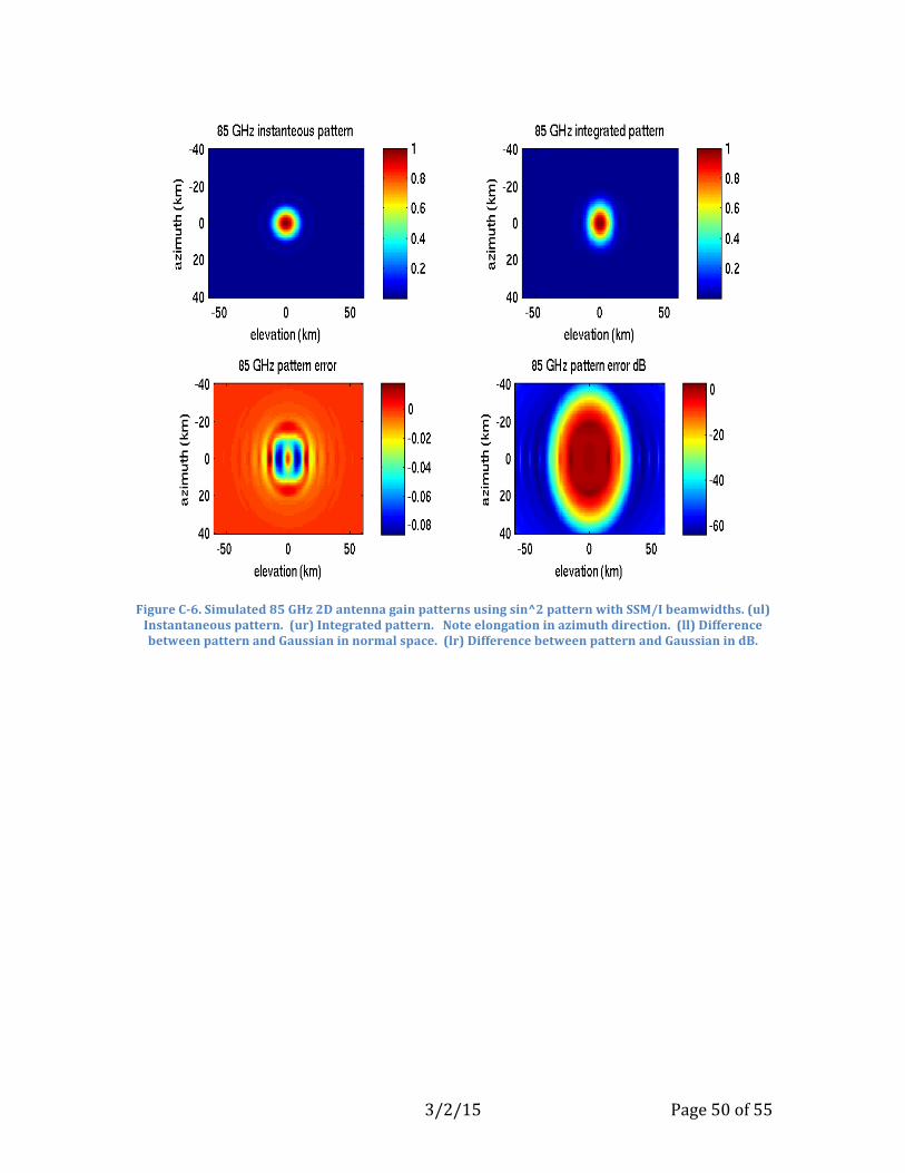
Note that the antenna patterns, when measured in degrees, are nearly circular. The integrated patterns are elongated in the azimuth direction. The projected antenna patterns are elongated in the elevation direction. Integration elongates the projected patterns in the azimuth direction, resulting in a nearly circular SRF at 19 GHz, with elliptical SRFs at 37 and 85 GHz.

3/2/15 Page 45 of 55
Figure C-1. Simulated 19 GHz antenna gain pattern slices using sin^2 pattern with SSM/I beamwidths.
(upper two panels) Azimuth. (lower two panels) Elevation. (top and third panels) The red line shows the ideal instantaneous antenna pattern. The blue line shows a slice through the azimuthally integrated
pattern for a single measurement. The green line is a Gaussian approximation to the grain pattern where the Gaussian 3dB width is the same as the antenna pattern. The dotted black line shows the dual-
Gaussian approximation. (second and fourth panels) The blue line shows the difference between the gain pattern and Gaussian approximation. The black line is the difference between the pattern and
dual-Gaussian.

3/2/15 Page 46 of 55
Figure C-2. Simulated 37 GHz antenna gain pattern slices. See caption for Fig. C-1 for explanation of
lines.

3/2/15 Page 47 of 55
Figure C-3. Simulated 37 GHz antenna gain pattern slices. See caption for Fig. C-1 for explanation of
lines.

3/2/15 Page 48 of 55
Figure C-4. Simulated 19 GHz 2D antenna gain patterns using sin^2 pattern with SSM/I beamwidths. (ul) Instantaneous pattern. (ur) Integrated pattern. Note elongation in azimuth direction. (ll) Difference between pattern and Gaussian in normal space. (lr) Difference between pattern and Gaussian in dB.

3/2/15 Page 49 of 55
Figure C-5. Simulated 37 GHz 2D antenna gain patterns using sin^2 pattern with SSM/I beamwidths. (ul) Instantaneous pattern. (ur) Integrated pattern. Note elongation in azimuth direction. (ll) Difference between pattern and Gaussian in normal space. (lr) Difference between pattern and Gaussian in dB.
3/2/15 Page 50 of 55
Figure C-6. Simulated 85 GHz 2D antenna gain patterns using sin^2 pattern with SSM/I beamwidths. (ul) Instantaneous pattern. (ur) Integrated pattern. Note elongation in azimuth direction. (ll) Difference between pattern and Gaussian in normal space. (lr) Difference between pattern and Gaussian in dB.

3/2/15 Page 51 of 55
Figure C-7. Simulated 19 GHz sine-squared antenna gain pattern slices projected on to the Earth’s
surface. (upper two panels) Azimuth. (lower two panels) Elevation. (top and third panels) The red line shows the ideal instantaneous antenna pattern. The blue line shows a slice through the azimuthally integrated pattern for a single measurement. The green line is a Gaussian approximation to the grain pattern where the Gaussian 3dB width is the same as the antenna pattern. (second and fourth panels)
The blue line shows the difference between the gain pattern and Gaussian approximation.

3/2/15 Page 52 of 55
Figure C-8. Simulated 37 GHz antenna gain pattern slices projected on to the Earth’s surface. See caption
for Fig. C-7.

3/2/15 Page 53 of 55
Figure C-9. Simulated 85 GHz antenna gain pattern slices projected on to the Earth’s surface. See caption
for Fig. C-7.

3/2/15 Page 54 of 55
Figure C-10. Simulated 19 GHz 2D antenna gain patterns projected onto the Earth’s surface. (ul) Instantaneous projected antenna pattern. (ur) Integrated pattern, i.e., the SRF. (ll) Difference between
SRF and Gaussian in normal space. (lr) Difference between SRF and Gaussian in dB.
Figure C-11. Simulated 37 GHz 2D antenna gain patterns projected onto the Earth’s surface. (ul) Instantaneous projected antenna pattern. (ur) Integrated pattern, i.e., the SRF. (ll) Difference between
SRF and Gaussian in normal space. (lr) Difference between SRF and Gaussian in dB.

3/2/15 Page 55 of 55
Figure C-12. Simulated SSM/I 85 GHz 2D antenna gain patterns projected onto the Earth’s surface. (ul) Instantaneous projected antenna pattern. (ur) Integrated pattern, i.e., the SRF. (ll) Difference between
SRF and Gaussian in normal space. (lr) Difference between SRF and Gaussian in dB.