animprovedmodelforhydromechanicalcouplingduring...

International Journal of Rock Mechanics & Mining Sciences 38 (2001) 317–329

An improved model for hydromechanical coupling duringshearing of rock joints

R. Olssona,*,1, N. Bartonb

aStatkraft Grøner AS, P.O. Box 400, N-1327 Lysaker, NorwaybNick Barton and Associates, Oslo, Norway and Sao Paulo, Brazil

Accepted 13 December 2000

Abstract

This paper presents some experimental results from hydromechanical shear tests and an improved version of the original modelsuggested by Barton (Office of Nuclear Waste Isolation, Columbus, Ohio, ONWI-308, 1982. 96pp.) for the hydromechanicalcoupling of rock joints. The original model was developed for coupling between mechanical and hydraulic aperture change duringnormal loading and unloading. The method was also suggested for the coupling of shear dilation and hydraulic aperture changes.

The improved model has the same appearance as the original and is based on hydromechanical shear experiments on granite rockjoints. It includes both the mechanical and hydraulic aperture and the mobilised joint roughness coefficient (JRCmob). # 2001Elsevier Science Ltd. All rights reserved.

1. Introduction

As a consequence of engineering works in a rockmass, deformation of both the joints and intact rock willusually occur as a result of the stress changes. Examplesof such works are repositories for radioactive waste,dam foundations, excavation of tunnels and caverns,geothermal energy plants, oil and gas production, etc.Due to the stiffer rock matrix, most deformation occursin the joints, in the form of normal and sheardisplacement. If the joints are rough, deformations willalso change the joint aperture and fluid flow.Traditionally, fluid flow through rock joints has been

described by the cubic law, which follows the assumptionthat the joints consist of two smooth, parallel plates. Realrock joints, however, have rough walls and variableaperture, as well as asperity areas where the two opposingsurfaces of the joint walls are in contact with each other.According to this, apertures can generally be defined

as mechanical (geometrically measured such as withepoxy injection) or hydraulic (measured by analysis ofthe fluid flow).

1.1. Mechanical aperture (E)

The mechanical joint aperture (E) is defined as theaverage point-to-point distance between two rock jointsurfaces (see Fig. 1), perpendicular to a selected plane. Ifthe joint surfaces are assumed to be parallel in the x2yplane, then the aperture can be measured in the zdirection. Often, a single, average value is used to definethe aperture, but it is also possible to describe itstochastically. The aperture distribution of a joint isonly valid at a certain state of rock stress and porepressure. If the effective stress and/or the lateral positionbetween the surfaces changes, as during shearing, theaperture distribution will also be changed.Usually, the mechanical aperture is determined from a

two-dimentional (2-D) joint section, which is a partcompound of the real 3-D surface.

1.2. Hydraulic aperture

The hydraulic aperture (e) can be determined bothfrom laboratory fluid-flow experiments [1–4], and bore-hole pump tests in the field [5,6].Fluid flow through rock joints is often represented

(assumed) as laminar flow between two parallel plates.The equivalent, smooth wall hydraulic aperture (e) can

1Formerly at Chalmers University of Technology, Gothenburg,

Sweden.

*Corresponding author. Tel.: +47-6712-8000; fax: +47-6712-8212.

E-mail address: [email protected] (R. Olsson).

1365-1609/01/$ - see front matter # 2001 Elsevier Science Ltd. All rights reserved.

PII: S 1 3 6 5 - 1 6 0 9 ( 0 0 ) 0 0 0 7 9 - 4

be obtained from flow tests using the modified form ofDarcy’s law relating flow rate (Q) and gradient (dP=dy):

Q ¼ g

nwe3

12

dP

dy; ð1Þ

where w is the width of the flow path and n is thekinematic viscosity. This relation is also called the‘‘cubic law’’. Here, only a single value is obtained for theaperture and the validity of Eq. (1) for natural rockjoints, has been discussed by many authors.An important distinction has to be made between the

theoretical smooth wall hydraulic aperture (e) and thereal mechanical aperture (E) (geometrically measured)between two irregular joint walls (Fig. 1). Owing to thewall friction and the tortuosity, E is generally largerthan e during normal loading and unloading, whichmeans that a rough joint requires a larger aperturethan a smooth joint for the same water conductingcapacity [7].

1.3. Fluid flow

The fluid flow in a rock mass is usually governed bythree factors: the fluid properties, the void geometry andthe fluid pressure at the joint boundary. The voidgeometry, i.e. the geometry of the volume between thejoint surfaces, is governed by the geological history andcan be described by several geometrical parameters, asaperture, frequency distribution, spatial correlation andcontact area [8]. These geometrical parameters arerelated in various ways to the joint void geometry, asshown in Fig. 2.Briefly, the properties can be described as follows:

* Aperture} the separation between the two joint wallsurfaces.

* Roughness } the surface height distribution or theshape of the surfaces.

* Contact area } the area where the surfaces are incontact, and can transfer stresses.

* Matedness } how well matched the surfaces are.* Spatial correlation } how abruptly or slowly theaperture changes from one point to another.

* Tortuosity } the forced bending of the stream linesdue to variations in joint aperture.

* Channelling } differences in flow velocity alongcertain paths, due to variations in joint aperture.

* Stiffness} the stiffness or mechanical properties of ajoint, which may be studied by looking at the closurecaused by applied normal load.

1.4. Hydromechanical coupling

In a rock mass, mechanical deformations will mainlyoccur as normal and/or shear deformations in the joints.This deformation will also change the joint aperture.By coupling the mechanical aperture changes to thehydraulic aperture changes, a hydromechanical couplingis achieved.Most research concerning hydromechanical coupling

in rock joints has been focused on the connectionbetween normal loading and unloading and their effecton joint conductivity. The fact that shearing of rockjoints can give an increasing or decrease of jointconductivity was highlighted during the InternationalSymposium ‘‘Percolation through fissured rock’’ in 1972[9–11].Perhaps, one of the first flow experiments under

concurrent shearing was performed on a cleavage planein slate, and was reported by Sharp and Maini [10].During the tests, no normal stress was applied, exceptfor the dead weight; the joint was thus free to dilate.After a shear displacement of around 0.7mm, theconductivity had increased by two orders of magnitude.In the laboratory environment, hydromechanical

shear experiments on joints with a normal stress higherthan the dead weight were first reported by Makurat [12]at the Norwegian Geotechnical Institute (NGI). The testperformed on a joint in gneiss with a constant waterhead of 2.8m and with an effective normal stress of0.82MPa showed an increase of the permeability by twoto three orders of magnitude after a shear displacementof around 1mm. In the field, Hardin et al. [13] had

Fig. 1. Definition of mechanical joint aperture.

Fig. 2. Fracture (herein=joint) properties determined by fracture void

geometry [8].

R. Olsson, N. Barton / International Journal of Rock Mechanics & Mining Sciences 38 (2001) 317–329318

reported minor increases in conducting aperture whenattempting to shear a diagonal joint in a 2� 2� 2mblock test in quartz monzonite gneiss. However, thejoint concerned was very rough and the block wasattached at its base.A constitutive model relating the hydraulic aperture

(e) with the real mechanical aperture (E) and the jointroughness (JRC) was proposed by Barton [14] andBarton, Bandis and Bakhtar [15]. The model wasdeveloped for coupling between mechanical and hy-draulic aperture changes during normal loading andunloading and also for dilatent shearing of rock joints.Unfortunately, it seems that this is the only equation forhydromechanical coupling during shear of rock joints.Based on new hydromechanical shear experiments on

granite rock joints [16,17] an improved empirical modelwill be suggested for shearing, dilatant joints. It has thesame appearance as the original and includes boththe mechanical (E) and hydraulic (e) aperture. However,the mobilised Joint Roughness Coefficient (JRCmob) [14]is used in place of JRCpeak.

2. Joint aperture } fluid flow and hydromechanical

coupling

Fluid flow through a porous medium such as manysoils and sedimentary rocks, can be described by Darcy’slaw (1-D flow):

Q ¼ KiA; ð2Þ

where Q is the volumetric flow per unit area A, normalto the flow. Q is thus related to the dimensionlesshydraulic gradient i, in the direction of the flow and tothe hydraulic conductivity K. The latter is a materialproperty of both the fluid and the geological mediumand may be written as

K ¼ krgm

; ð3Þ

where k is the intrinsic permeability, g is the accelerationdue to gravity (9.81m/s2), m is the dynamic viscosity ofthe fluid (1� 10�3N s/m2 for pure water at 208C) and ris the fluid density (998 kg/m3 for pure water at 208C).For fluid flow through rock joints, it is common to

consider the joint as composed of two smooth parallelplates and the flow to be steady, single phase, laminarand incompressible. Under these conditions, the hy-draulic joint conductivity (Kj) may be written (afterPoiseulle):

Kj ¼rgm

e2

12ð4Þ

or

Kj ¼ge2

12n; ð5Þ

where n is the kinematic viscosity of the fluid(1.0� 10�6m2/s for pure water at 208C) and e is thehydraulic aperture. The hydraulic joint conductivity is aparameter expressing the flow through the joint underthe influence of frictional losses, tortuosity and channel-ling; these factors depend on the geometry of the flowchannels and the fluid viscosity. Assuming that Darcy’slaw (Q ¼ KiA) can also be applied to flow in rock joints,setting A ¼ ew, we obtain

Q ¼ g

nwe3

12i; ð6Þ

where i is the dimensionless hydraulic gradient and w isthe breadth of the flowing zone between the parallelplates. This equation is usually called the ‘‘cubic law’’.One must keep in mind that Eq. (6) is derived for an‘‘open’’ channel, i.e. the planar surfaces remain paralleland are thus not in contact at any point.When Darcys’s law is applied to natural rock joints

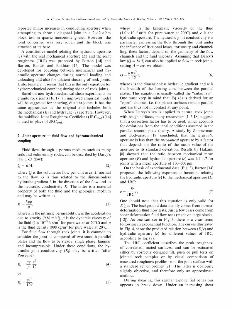
with rough surfaces, many researchers [1–3,18] suggeststhat a correction factor has to be used, which accountsfor deviations from the ideal conditions assumed in theparallel smooth plate theory. A study by Zimmermanand Bodvarsson [19] concluded, that the hydraulicaperture is less than the mechanical aperture by a factorthat depends on the ratio of the mean value of theaperture to its standard deviation. Results by Hakami[8] showed that the ratio between mechanical meanaperture (E) and hydraulic aperture (e) was 1.1–1.7 forjoints with a mean aperture of 100–500 mm.On the basis of experimental data (Fig. 3), Barton [14]

proposed the following exponential function, relatingthe hydraulic aperture (e) to the mechanical aperture (E)and JRC:

e ¼ E2

JRC2:5ð7Þ

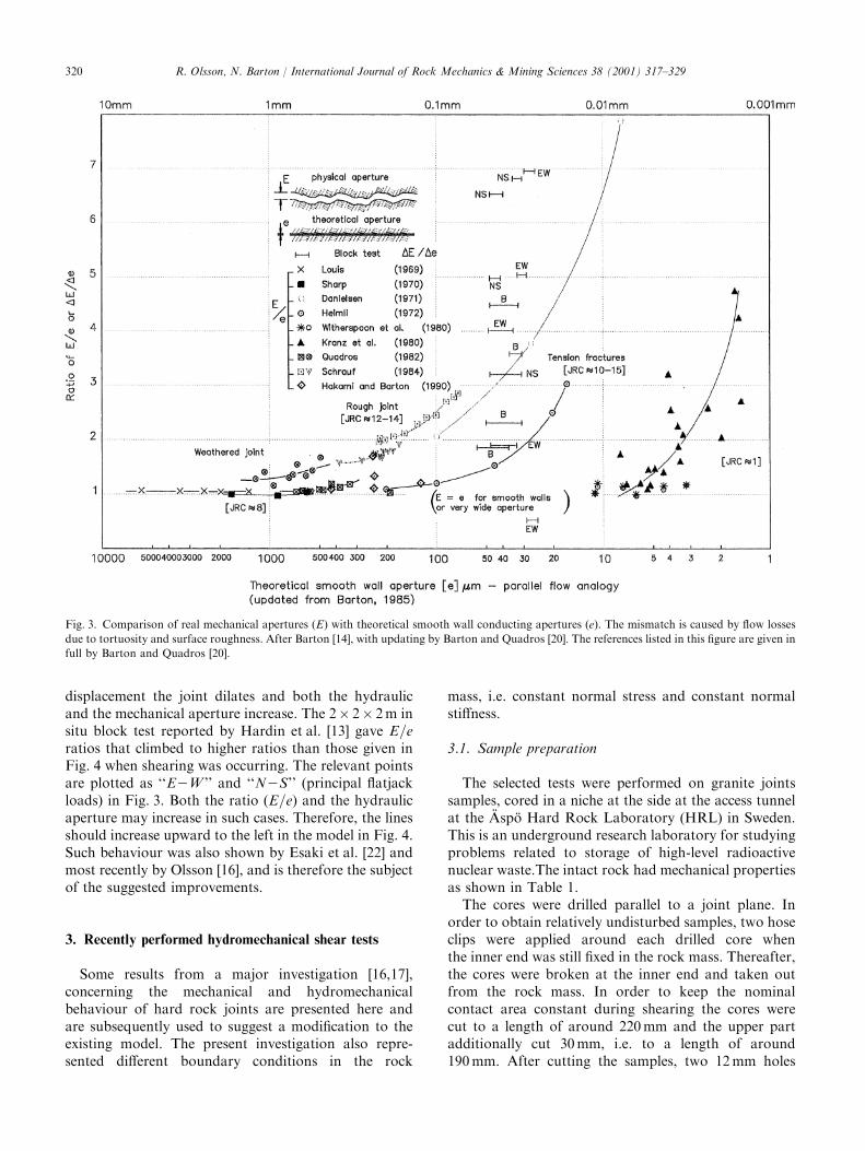
One should note that this equation is only valid forE � e. The background data mainly comes from normaldeformation fluid flow tests. Just a few cases come fromshear deformation fluid flow tests (made on large blocks,[12]). As one can see in Fig. 3, there is a clear trendfollowing an exponential function. The curves illustratedin Fig. 4, show the predicted relation between (E=e) andhydraulic aperture (e) for different values of JRC,according to Eq. (7).The JRC coefficient describes the peak roughness

of correlated, mated surfaces, and can be estimatedeither by correctly designed tilt, push or pull tests onjointed rock samples or by visual comparison ofmeasured roughness profiles from the joint surface witha standard set of profiles [21]. The latter is obviouslyslightly objective, and therefore only an approximatemethod.During shearing, this regular exponential behaviour

appears to break down. Under an increasing shear

R. Olsson, N. Barton / International Journal of Rock Mechanics & Mining Sciences 38 (2001) 317–329 319

displacement the joint dilates and both the hydraulicand the mechanical aperture increase. The 2� 2� 2m insitu block test reported by Hardin et al. [13] gave E=eratios that climbed to higher ratios than those given inFig. 4 when shearing was occurring. The relevant pointsare plotted as ‘‘E2W ’’ and ‘‘N2S’’ (principal flatjackloads) in Fig. 3. Both the ratio (E=e) and the hydraulicaperture may increase in such cases. Therefore, the linesshould increase upward to the left in the model in Fig. 4.Such behaviour was also shown by Esaki et al. [22] andmost recently by Olsson [16], and is therefore the subjectof the suggested improvements.

3. Recently performed hydromechanical shear tests

Some results from a major investigation [16,17],concerning the mechanical and hydromechanicalbehaviour of hard rock joints are presented here andare subsequently used to suggest a modification to theexisting model. The present investigation also repre-sented different boundary conditions in the rock

mass, i.e. constant normal stress and constant normalstiffness.

3.1. Sample preparation

The selected tests were performed on granite jointssamples, cored in a niche at the side at the access tunnelat the Aspo Hard Rock Laboratory (HRL) in Sweden.This is an underground research laboratory for studyingproblems related to storage of high-level radioactivenuclear waste.The intact rock had mechanical propertiesas shown in Table 1.The cores were drilled parallel to a joint plane. In

order to obtain relatively undisturbed samples, two hoseclips were applied around each drilled core whenthe inner end was still fixed in the rock mass. Thereafter,the cores were broken at the inner end and taken outfrom the rock mass. In order to keep the nominalcontact area constant during shearing the cores werecut to a length of around 220mm and the upper partadditionally cut 30mm, i.e. to a length of around190mm. After cutting the samples, two 12mm holes

Fig. 3. Comparison of real mechanical apertures (E) with theoretical smooth wall conducting apertures (e). The mismatch is caused by flow losses

due to tortuosity and surface roughness. After Barton [14], with updating by Barton and Quadros [20]. The references listed in this figure are given in

full by Barton and Quadros [20].


were cored at each end of the lower specimen, two forinlet and two for outlet of water. In the holes, 10mmcopper pipes were then placed, and the two specimenparts were cast into larger concrete blocks to fit in theshear box holders.The joint roughness, via the JRC, was determined

from back-calculation of the shear tests, while the basicfriction angle was estimated from shear tests performedon samples with saw-cut, dry surfaces. Tests performedwith a Schmidt hammer showed that the JCS valuecould be set equal to the uniaxial compressive strength.The initial test parameters and joint properties areshown in Table 2.After preparation and characterisation of the samples,

hydromechanical direct shear tests were performed inthe shear equipment at Lulea University of Technology,Sweden.

3.2. Experimental equipment

The direct shear experiments were performed withservo-hydraulic equipment. In principle, the equipment

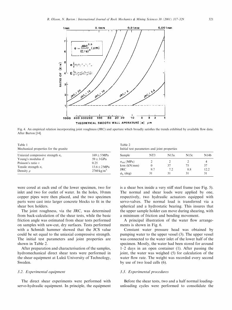
is a shear box inside a very stiff steel frame (see Fig. 5).The normal and shear loads were applied by one,respectively, two hydraulic actuators equipped withservo-valves. The normal load is transferred via aspherical and a hydrostatic bearing. This insures thatthe upper sample holder can move during shearing, witha minimum of friction and bending movement.A principal illustration of the water flow arrange-

ments is shown in Fig. 6.Constant water pressure head was obtained by

pumping water to the upper vessel (3). The upper vesselwas connected to the water inlet of the lower half of thespecimen. Mostly, the water had been stored for around1–2 days in an open container (1). After passing thejoint, the water was weighed (5) for calculation of thewater flow rate. The weight was recorded every secondby use of two load cells (6).

3.3. Experimental procedures

Before the shear tests, two and a half normal loading-unloading cycles were performed to consolidate the

Fig. 4. An empirical relation incorporating joint roughness (JRC) and aperture which broadly satisfies the trends exhibited by available flow data.

After Barton [14].

Table 1

Mechanical properties for the granite

Uniaxial compressive strength sc 169� 5MPaYoung’s modulus E 59� 3GPaPoisson’s ratio n 0.25

Tensile strength st 13.6� 2MPaDensity r 2760 kg/m3

Table 2

Initial test parameters and joint properties

Sample NT3 N13a N13c N14b

sinit:ðMPaÞ 2 2 2 4

krm (kN/mm) 0 37 75 37

JRC 9.7 7.2 8.8 12.2

fb (deg) 31 31 31 31


joints. The maximum load was the same as later used forthe shear tests.The shear tests were performed at two normal stresses

(sn ¼ 2 and 4MPa) and with three loading conditions;constant normal load (CNL) where the rock massstiffness krm ¼ 0, and constant normal stiffness (CNS)where the rock mass stiffness krm was either 37 or 75 kN/mm. In the CNL tests, the joint was allowed to dilate

with no increase of the normal load, while during theCNS tests, a hydraulic spring load provided constantnormal stiffness [16]. The load was linearly proportionalto the normal displacement and was measured by fourgauges at a given constant normal stiffness. After a totalshear movement of around 15mm, the shear movementwas stopped and the normal load removed.At the ‘‘upstream’’ end of the joints, a water pressure

head of 4m was applied. After passing the inlet pipes, thewater were evenly distributed over the whole width ofthe joint. At the ‘‘downstream’’ end of the joints thewater was collected and weighed for flow rate estimation.

3.4. Experimental results and analysis

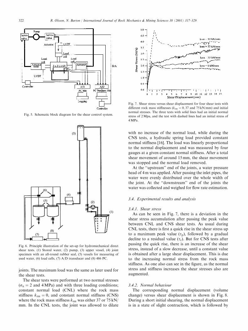
3.4.1. Shear stressAs can be seen in Fig. 7, there is a deviation in the

shear stress accumulation after passing the peak valuebetween CNL and CNS shear tests. As usual duringCNL tests, there is first a quick rise in the shear stress upto a maximum peak value (tp), followed by a gradualdecline to a residual value (tr). But for CNS tests afterpassing the quick rise, there is an increase of the shearstress, instead of a slow decrease, until a constant valueis obtained after a large shear displacement. This is dueto the increasing normal stress from the rock massstiffness. As one also can see in the figure, as the normalstress and stiffness increases the shear stresses also areaugmented.

3.4.2. Normal behaviourThe corresponding normal displacement (volume

change) versus shear displacement is shown in Fig. 8.During a short initial shearing, the normal displacementis in a state of slight contraction, which is followed by

Fig. 5. Schematic block diagram for the shear control system.

Fig. 6. Principle illustration of the set-up for hydromechanical direct

shear tests. (1) Stored water, (2) pump, (3) upper vessel, (4) joint

specimen with an all-round rubber seal, (5) vessels for measuring of

used water, (6) load cells, (7) A/D transducer and (8) 486 PC.

Fig. 7. Shear stress versus shear displacement for four shear tests with

different rock mass stiffnesses (krm ¼ 0; 37 and 75 kN/mm) and initialnormal stresses. The three tests with solid lines had an initial normal

stress of 2Mpa, and the test with dashed lines had an initial stress of

4MPa.


dilation. The maximum normal displacement occursas the shear stress attains a residual value, but themaximum rate of dilation corresponds to the prelimin-ary peak shear strength. Due to the increasing normalstress during CNS tests, the dilation is less for CNS thanfor CNL.

3.4.3. Stress paths during shearingConcerning the stress paths shown in Fig. 9, the CNL

and CNS tests exhibit differences.In each case, the shear stress rises to a preliminary

peak. In the CNS tests, the shear stress then slowly risesfurther while in the CNL test it falls to a preliminaryresidual value of shear stress. The maximum value iscommonly used for estimation of a shear strength curve.In Fig. 9, the peak shear strength value for CNL test ismarked with a triangle.Peak shear strength curves were calculated according to

tp ¼ sn tan JRC log10JCS

sn

� �þ fr

� �; ð8Þ

where sn is the normal stress, and fr is the residualfriction angle. These are shown as fine dotted curves inFig. 9. To generate these curves, it has been assumed thatJCS=sc=215MPa and fr ¼ fb ¼ 328. Four differentvalues of JRC have been used. These envelopes corre-spond best with the peak value for the CNL test but alsoquite well for the CNS tests.

3.4.4. Hydromechanical behaviourThe most evident hydromechanical coupling during

the shear tests is between the shear displacement and thetransmissivity (T). The transmissivity is defined as

T ¼ Q

wi: ð9Þ

The transmissivity is seen to increase at least an order ofmagnitude with 4 or 5mm of shearing in all the casesstudied. As one can see in Fig. 10, the transmissivitydecreased with higher rock mass stiffness and initialnormal stress because joints suffer a normal stressincrease under CNS tests.

3.4.5. Mechanical and hydraulic apertureIn order to plot the changes of the mechanical aperture

versus the hydraulic aperture during shear deformation(Fig. 11), we first assumed that the changes of themechanical aperture are equal to the dilation of the rockjoint. The mechanical aperture (E ¼ E0þDE) was calcu-lated by adding the changes of dilation (DE) to an initialaperture (E0) equal to the mechanical aperture at the endof the normal loading cycles. No real initial mechanicalaperture were measured, only closure/opening of thejoints. As the initial mechanical aperture not was measuredbefore the shear tests, the final hydraulic aperture from theloading/unloading tests was used for estimations usingEq. (7). Thereafter, ratios of E=e were calculated for each0.5mm interval and plotted versus e in Fig. 12.In Fig. 11, the mechanical aperture and the hydraulic

aperture versus shear displacement are plotted for thefour tests. As one can see in the figure, the increase inmechanical aperture is greater than that of the hydraulicaperture after passing the peak shear stress (obtained ataround 1–2mm shear displacement).

Fig. 8. Normal displacement versus shear displacement for four shear

tests showed in Fig. 7.

Fig. 9. Shear stress versus effective normal stress for four shear tests

showed in Fig. 7.

Fig. 10. Transmissivity versus shear displacement for the four shear

tests shown in Fig. 7.


For predictions of fluid flow in hydraulic models thehydraulic aperture is obviously used. However, duringnumerical modelling of rock mass deformation, using forexample the distinct element UDEC code [23], the jointopening or closing is first calculated. When shearing doesnot occur, conversion between mechanical aperture andhydraulic aperture can follow the trends shown in Figs. 3and 4. However, when shearing and dilation occur, theinterlocking asperity geometry begins to breakdown.As one can see in the Fig. 12, E=e increases in a

reversed manner, compared to the other curves in thefigure. This was expected, following the results inFig. 11; however, it is contrary to what was suggestedin the original model [14], which was mostly based onnormal closure-flow coupling data (see Fig. 3). Such a

deviation, was also shown by Esaki et al. [22] and byBarton [14] as mentioned earlier. However, a goodexplanation was not developed.In the case of Esaki et al. [22] tests, the joints in

sandstone were loaded to more than 50% of the uniaxialcompression strength. Production of gouge probablycaused the high E=e ratios (maximum E=e=25). Gougeproduction also caused some CSFT (coupled shear-flowtests) reported by Makurat et al. [24] to show reducedpermeability in relation to the predicted (maximum)effect of dilation. The original E=e versus JRC model[14] is in fact almost exclusively based on normalcompression or opening tests and comparisons betweentrue (measured) mechanical apertures and hydraulicapertures. During increased normal stress, the hydraulicaperture (e) decreases, which causes an increase in E=edue to tortuosity. This behaviour tends to follow the‘‘JRC0 curves’’ in Fig. 4.During the first part of each plotted shear path in

Fig. 12, the E=e ratio is first slightly decreasing andthereafter increasing. This initial part belongs to the pre-peak and peak shear displacement when the aspertiesalong the joint walls are not destroyed and the hydraulicaperture is probably decreasing due to shear-relatedclosing of small voids. Thereafter, the geometry ofthe joint walls is in a changing phase, (the so-called‘‘breakdown’’) where the asperities get worn anddamaged under the increasing shear deformation. Thesize of roughness degradation (decrease in mobilizedJRC) depends on the strength of the asperities, on theapplied normal load and on the shear deformation.Furthermore, new flow paths open and others close dueto the increasing areas of contact between the joint wallsand due to gouge production. For this behaviour, aconceptual model visualising reduction of joint porositywith increasing gouge production has been suggested[20]. The gouge production will probably decrease thehydraulic aperture. So, the increase in E=e duringshearing depends not on the same phenomena as duringnormal loading and unloading. In the recent literature,some reported tests [25,26] have shown that after passingthe peak displacement, the principal flow paths mayreorient and become directed nearly perpendicular to theshear direction. This is not incorporated in the model atpresent, as it may not be a general result. Conceptually,it is difficult to imagine elongated areas of wear allowinggreater perpendicular flow. However, if the elongationsof constant areas are oriented perpendicular to the sheardirection, such could be readily understood.

4. A model for hydromechanical coupling during shearing

of rock joints

An improved model is therefore proposed on the basisof the performed hydromechanical shear tests [11] and

Fig. 11. Measured joint closure and calculated hydraulic aperture

versus shear displacement for hydromechanical direct shear tests.

Fig. 12. Calculated E=e versus e for the tests in Fig. 4 in a diagram

suggested by Barton [14]. Breakdown is indicated, due to the shearing.


based on the above discussion. It is an empiricalengineering model and not a theoretical scientific modeland is built on the E=e versus e curves for the four testsreviewed before. Further, it is not a reversible model. Asshear tests on rough rock joints are composed of at leasttwo major parts, pre-peak/peak and post-peak, themodel considers these two basic phases. For the firstphase, the coupling between the mechanical andhydraulic aperture assumes more or less interlocked,matched joint walls. This starting value of the hydraulicaperture is the final value from the normal loading cycleand can be calculated by Eq. (7):

e ¼ JRC2:50

ðE=eÞ2:

This ‘‘starting point’’ applies also to shear displacementðusÞ 0:75usp (peak shear displacement).The second phase for us � usp can be calculated by

e ¼ E

e

� �JRC2mob: ð10Þ

Eq. (10) applies to values of JRCmob > 0, i.e. joints withfinite roughness (JRC0 > 0) and with a residual rough-ness despite shearing. In the first phase, where the jointwall roughness is not destroyed, the peak JRC0 shouldbe used. In the second phase, were the geometry of thejoint walls is changing with increasing shear displace-ment, the JRCmob (mobilized value of JRC) should beused [14]. During this phase, gouge is being producedbut as the joint is dilating some of the gouge is probablyflushed to the sides of developing flow channels. Thevalue of JRCmob is dependent on the strength on thejoint surface (JCS), on the applied normal stress (sn)and on the magnitude of the shear displacement. Itis also dependent on the size of joint plane (Ln) andon the residual friction angle (fr). The intermediatephase, between phase one and two (us ¼ 0:75usp to usp),is difficult to define with any model and it isrecommended for the present that the two phases areconnected with each other by a transition curve.For the calculations of JRCmob the following relevant

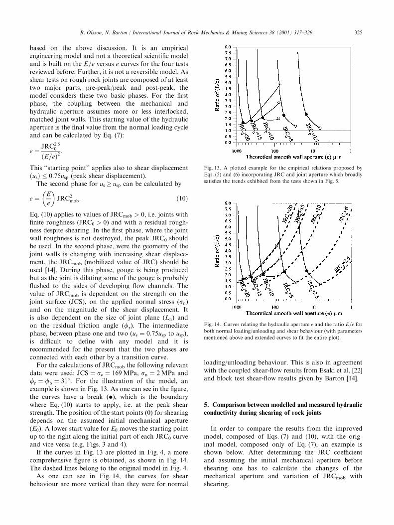
data were used: JCS ¼ sc ¼ 169MPa, sn ¼ 2MPa andfr ¼ fb ¼ 318. For the illustration of the model, anexample is shown in Fig. 13. As one can see in the figure,the curves have a break (*), which is the boundarywhere Eq. (10) starts to apply, i.e. at the peak shearstrength. The position of the start points (0) for shearingdepends on the assumed initial mechanical aperture(E0). A lower start value for E0 moves the starting pointup to the right along the initial part of each JRC0 curveand vice versa (e.g. Figs. 3 and 4).If the curves in Fig. 13 are plotted in Fig. 4, a more

comprehensive figure is obtained, as shown in Fig. 14.The dashed lines belong to the original model in Fig. 4.As one can see in Fig. 14, the curves for shear

behaviour are more vertical than they were for normal

loading/unloading behaviour. This is also in agreementwith the coupled shear-flow results from Esaki et al. [22]and block test shear-flow results given by Barton [14].

5. Comparison between modelled and measured hydraulic

conductivity during shearing of rock joints

In order to compare the results from the improvedmodel, composed of Eqs. (7) and (10), with the orig-inal model, composed only of Eq. (7), an example isshown below. After determining the JRC coefficientand assuming the initial mechanical aperture beforeshearing one has to calculate the changes of themechanical aperture and variation of JRCmob withshearing.

Fig. 13. A plotted example for the empirical relations proposed by

Eqs. (5) and (6) incorporating JRC and joint aperture which broadly

satisfies the trends exhibited from the tests shown in Fig. 5.

Fig. 14. Curves relating the hydraulic aperture e and the ratio E=e for

both normal loading/unloading and shear behaviour (with parameters

mentioned above and extended curves to fit the entire plot).


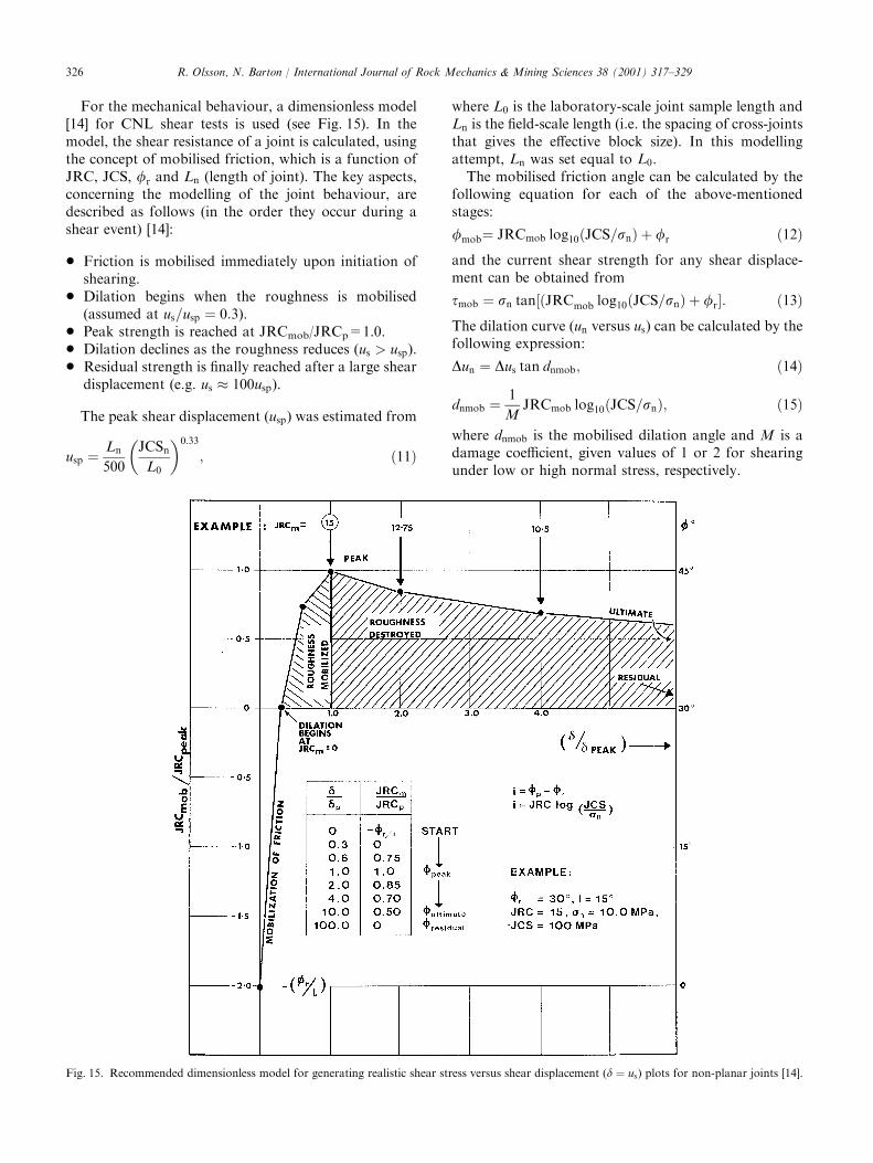
For the mechanical behaviour, a dimensionless model[14] for CNL shear tests is used (see Fig. 15). In themodel, the shear resistance of a joint is calculated, usingthe concept of mobilised friction, which is a function ofJRC, JCS, fr and Ln (length of joint). The key aspects,concerning the modelling of the joint behaviour, aredescribed as follows (in the order they occur during ashear event) [14]:

* Friction is mobilised immediately upon initiation ofshearing.

* Dilation begins when the roughness is mobilised(assumed at us=usp ¼ 0:3).

* Peak strength is reached at JRCmob/JRCp=1.0.* Dilation declines as the roughness reduces (us > usp).* Residual strength is finally reached after a large sheardisplacement (e.g. us 100usp).

The peak shear displacement (usp) was estimated from

usp ¼Ln500

JCSnL0

� �0:33; ð11Þ

where L0 is the laboratory-scale joint sample length andLn is the field-scale length (i.e. the spacing of cross-jointsthat gives the effective block size). In this modellingattempt, Ln was set equal to L0.The mobilised friction angle can be calculated by the

following equation for each of the above-mentionedstages:

fmob¼ JRCmob log10ðJCS=snÞ þ fr ð12Þand the current shear strength for any shear displace-ment can be obtained from

tmob ¼ sn tan½ðJRCmob log10ðJCS=snÞ þ fr�: ð13ÞThe dilation curve (un versus us) can be calculated by thefollowing expression:

Dun ¼ Dus tan dnmob; ð14Þ

dnmob ¼1

MJRCmob log10 JCS=snð Þ; ð15Þ

where dnmob is the mobilised dilation angle and M is adamage coefficient, given values of 1 or 2 for shearingunder low or high normal stress, respectively.

Fig. 15. Recommended dimensionless model for generating realistic shear stress versus shear displacement (d ¼ us) plots for non-planar joints [14].


For initial values of JRCmob/JRCp, the ratio �fr=iis used, where [14]

i¼ JRC log10ðJCS=snÞ: ð16ÞThereafter, the values of JRCmob/JRCp in the table inFig. 15 should be used.The hydraulic conductivity was calculated according

to

K ¼ ge2

12n; ð17Þ

where the hydraulic aperture was determined by Eq. (7)and by rewriting Eq. (10):

e ¼ E2

JRC2:50; us 0:75usp;

e ¼ffiffiffiffiE

pJRCmob; us � usp:

The mechanical aperture was calculated as

E ¼ E0 þ DE; ð18Þwhere DE (caused by joint dilation) can be taken as thetangent of the dilation angle (Eq. 14). A given incrementof shear displacement will result in a positive DEcomponent:

DE ¼ Dus tan dnmob: ð19ÞBy combining Eqs. (14) and (18) one can calculate themechanical aperture:

E ¼ E0 þ Dus tan1

MJRCmob log10ðJCS=snÞ

� �: ð20Þ

Usually, the mechanical aperture (E0) is the initialaperture when shearing starts.For comparison, only one of the hydromechanical

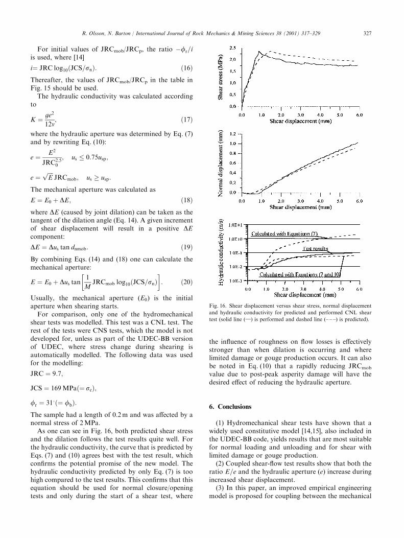
shear tests was modelled. This test was a CNL test. Therest of the tests were CNS tests, which the model is notdeveloped for, unless as part of the UDEC-BB versionof UDEC, where stress change during shearing isautomatically modelled. The following data was usedfor the modelling:

JRC ¼ 9:7;

JCS ¼ 169MPað¼ scÞ;

fr ¼ 318ð¼ fbÞ:The sample had a length of 0.2m and was affected by anormal stress of 2MPa.As one can see in Fig. 16, both predicted shear stress

and the dilation follows the test results quite well. Forthe hydraulic conductivity, the curve that is predicted byEqs. (7) and (10) agrees best with the test result, whichconfirms the potential promise of the new model. Thehydraulic conductivity predicted by only Eq. (7) is toohigh compared to the test results. This confirms that thisequation should be used for normal closure/openingtests and only during the start of a shear test, where

the influence of roughness on flow losses is effectivelystronger than when dilation is occurring and wherelimited damage or gouge production occurs. It can alsobe noted in Eq. (10) that a rapidly reducing JRCmobvalue due to post-peak asperity damage will have thedesired effect of reducing the hydraulic aperture.

6. Conclusions

(1) Hydromechanical shear tests have shown that awidely used constitutive model [14,15], also included inthe UDEC-BB code, yields results that are most suitablefor normal loading and unloading and for shear withlimited damage or gouge production.(2) Coupled shear-flow test results show that both the

ratio E=e and the hydraulic aperture (e) increase duringincreased shear displacement.(3) In this paper, an improved empirical engineering

model is proposed for coupling between the mechanical

Fig. 16. Shear displacement versus shear stress, normal displacement

and hydraulic conductivity for predicted and performed CNL shear

test (solid line (}) is performed and dashed line (– – –) is predicted).


and hydraulic aperture including the joint roughnesscoefficient (JRC) for predictions of fluid flow throughrock joints. The model consists of two parts which aredependent on the shear displacement:

e ¼ E2

JRC2:50; us 0:75usp;

e ¼ E1=2 JRCmob; us � usp:

(4) A first modelling attempt has shown a promising,improved agreement between the predicted andmeasured hydraulic conductivity for a hydromechanicalshear test performed on a granite joint sample. Despitethe fact that the model is proposed based on hydro-mechanical shear tests on granite rock joints, we alsorecommend its use on other rock types but with duecaution.(5) For engineering modelling of conductivity changes

of rock joints during shearing, one has therefore first toassume the initial JRC value and the initial mechanicalaperture. Thereafter, one has to calculate the changes ofthe mechanical aperture and JRCmob during shearing.This can be done with a dimensionless model for shearbehaviour. These parameters should then be used inEqs. (7) and (10) to calculate the changes of thehydraulic aperture during shearing. Thereafter, it ispossible to calculate either the hydraulic conductivity ortransmissivity.(6) Further work will be needed in order to

incorporate the improved model in the UDEC code.

Acknowledgements

The first author would like to thank the SwedishNuclear Fuel and Waste Management Company (SKB)for the financial support during the experimental phase,and also Gr�ner AS for support during writing of thispaper. The second author would like to thank nuclearwaste research funding by ONWI and AECL of theUSA and Canada, who supported our rock mechanicsdevelopments in the 1980s. Colleagues Bandis andBakhtar made special contributions.

References

[1] Witherspoon PA, Wang JSY, Iwai K, Gale JE. Validity of cubic

law for a deferrable rock fracture. Water Resources Res,

1980;16(6):1016–24.

[2] Elliot GM, Brown ET, Boodt PI, Hudson JA. Hydromechanical

behaviour of the Carnmenellis granite, S.W. England. In:

Stephansson O, editor. Conference Proceedings, International

Symposium on Fundamentals of Rock Joints. Sweden: Bjorkli-

den, 1985. p. 249–58.

[3] Zhao J, Brown ET. Hydro-thermo-mechanical properties of joints

in the Carnmenellis granite. Quart J Engng Geol 1992;25:279–90.

[4] Larsson E. Groundwater flow through a natural fracture } flow

experiments and numerical modelling. Licentiate Thesis,

Department of Geology, Chalmers University of Technology,

Gothenburg, Sweden, Publ. A 82, 1997.

[5] Pine RJ. Rock joint and rock mass behaviour during pressurised

hydraulic injection. Ph.D. Thesis, Camborne School of Mines,

Cornwall, UK, 1986.

[6] Rutqvist J. Coupled stress-flow properties of rock joints from

hydraulic field testing. Ph.D. Thesis, Division of Engineering

Geology, Royal Institute of Technology, Stockholm, 1995.

[7] Bandis SC. Engineering properties and characterization of rock

discontinuities. In: Comprehensive Rock Engineering. Principles,

Practice & Projects. vol. 1: Fundamentals, 1993. p. 155–18.

[8] Hakami E. Aperture distribution of rock fractures. Ph.D. Thesis,

Division of Engineering Geology, Royal Institute of Technology,

Stockholm, 1995.

[9] Sharp JC, Brawner CO. Prediction of the drainage properties of

rock masses. Theme 4, International Symposium on Percolation

through Fissured Rock, Stuttgart, 1972.

[10] Sharp JC, Maini YNT. Fundamental considerations on the

hydraulic characteristics of joints in Rock. Paper T1-F, Interna-

tional Symposium on Percolation through Fissured Rock,

Stuttgart, 1972.

[11] Barton N. The problem of joint shearing in coupled stress-flow

analyses. Discussion D4, International Symposium on Percola-

tion through Fissured Rock. Stuttgart, 1972.

[12] Makurat A. The effect of shear displacement on the permeability

of natural rough joints. Hydrogeology of rocks of low perme-

ability. Proceedings of the 17th International Congress on

Hydrogeology, Tucson, Arizona, USA, 1985. p. 99–106.

[13] Hardin EL, Barton N, Lingle R, Board MP, Voegele MD. A

heated flatjack test series to measure the thermomechanical and

transport properties of in situ rock masses. Office of Nuclear

Waste Isolation, Columbus, Ohio, ONWI-260, 1982. 193pp.

[14] Barton N. Modelling rock joint behaviour from in situ block tests:

implications for nuclear waste repository design. Office of Nuclear

Waste Isolation, Columbus, OH, ONWI-308, 1982. 96pp.

[15] Barton N, Bandis S, Bakhtar K. Strength, deformation and

conductivity coupling of rock joints. Int J Rock Mech Min Sci

Geomech Abstr 1985;22:121–40.

[16] Olsson R. Mechanical and hydromechanical behaviour of hard

rock joints } a laboratory study. Ph.D. thesis, Chalmers

University of Technology, Gothenburg, Sweden, 1998. p. 197.

[17] Olsson R. Mechanical and hydromechanical behaviour of hard

rock joints } a laboratory study. Addendum, Report 1999:6,

Chalmers University of Technology, Gothenburg, Sweden, 1999.

p. 34.

[18] Zhao J. Effect of normal stress and temperature on hydraulic

properties of rock fractures. Conference Proceedings on

Memories of the XXIV Congress of IAH, Oslo, Norway, 1993.

p. 115–22.

[19] Zimmerman RW, Bodvarsson GS. Hydraulic conductivity of rock

fractures. Transport Porous Media 1996;23:1–30.

[20] Barton N, Quadros EF. Joint aperture and roughness in the

prediction of flow and groutability of rock masses. Int J Rock

Mech Min Sci. 1997;34(3–4), Paper No. 252.

[21] Barton N, Choubey V. The shear strength of rock joints in theory

and practice. Rock Mech 1977;10:1–54.

[22] Esaki T, Ikusada K, Aikawa A, Kimura T. Surface roughness and

hydraulic properties of sheared rock. Fractured and Jointed Rock

Masses, Lake Tahoe, CA, 1995. p. 93–8.

[23] Cundall PA. A generalized distinct element program for model-

ling jointed rock. Report PCAR-1-80. Contract DAJA37-79-C-

0548, European Research Office, US Army, Peter Cundall

Associates, 1980.


[24] Makurat A, Barton N, Rad NS, Bandis S. Joint conductivity

variation due to normal and shear deformation. Proceedings of

the International Symposium on Rock Joints, Balkema, Loen,

Norway, 1990. p. 535–40.

[25] Gentier S, Lamontagne E, Archambault G, Riss J. Anisotropy of

flow in a fracture undergoing shear and its relationship to the

direction of shearing and injection pressure. Int J Rock Mech Min

Sci 1997;34(3–4), Paper No. 094.

[26] Gentier S, Riss J, Hopkins D, Lamontagne E. Hydromechanical

behaviour of a fracture: how to understand the flow paths.

Proceedings of the Third International Conference on Mechanics

of Jointed and Faulted Rock, Vienna, Austria, 1998. p. 405–22.


animprovedmodelforhydromechanicalcouplingduring...

Documents