angle estimation for two unresolved targets with …zjanew/journal/zjw_aes_aemonradar_23.pdf ·...

Angle Estimation for TwoUnresolved Targets withMonopulse Radar

ZHEN WANGUniversity of Maryland

ABHIJIT SINHA

PETER WILLETT, Fellow, IEEE

YAAKOV BAR-SHALOM, Fellow, IEEEUniversity of Connecticut

Most present-day radar systems use monopulse techniquesto extract angular measurements of subbeam accuracy. Thefamiliar “monopulse ratio” is a very effective means to derivethe angle of a single target within a radar beam. For thesimultaneous estimation of the angles of two closely-spacedtargets, a modification on the monopulse ratio was derived in [7],while [21] presented a maximum likelihood (ML) technique vianumerical search.In this paper it is shown that the ML solution can in fact be

found explicitly, and the numerical search of [21] is unnecessary.However, the ML solution requires the signal to noise ratio (SNR)for each target to be known, and hence we generalize it so itrequires only the relative SNR. Several versions of expectationmaximization (EM) joint angle estimators are also derived, thesediffering in the degree to which prior information on SNR and onbeam pattern are assumed.The performances of the different direction-of-arrival (DOA)

estimators for unresolved targets are studied via Monte Carlo,and it is found that most have similar performance: this isremarkable since the use of prior information (SNR, relative SNR,beam pattern) varies widely between them. There is, however,considerable performance variability as a function of the twotargets’ off-boresight angles. A simple combined technique thatfuses the results from different approaches is thus proposed, andit performs well uniformly.

Manuscript received April 12, 2003; revised February 5 and May 4,2004; released for publication May 28, 2004.

IEEE Log No. T-AES/40/3/835894.

Refereeing of this contribution was handled by L. M. Kaplan.

This work was supported by the Office of Naval Research.

Authors’ addresses: Z. Wang, Dept. of Electrical and ComputerEngineering, University of Maryland , College Park, MD 20742; A.Sinha, P. Willett, Y. Bar-Shalom, Dept. of Electrical and ComputerEngineering, U-2157, University of Connecticut, 371 Fairfield Rd.,Storrs, CT 06269-3157, E-mail: ([email protected]).

0018-9251/04/$17.00 c° 2004 IEEE

I. INTRODUCTION

Amplitude comparison monopulse (ACM, or“monopulse”) radar systems are quite commonlyused, and represent a practical and quick means toimprove the accuracy of angular measurements to afraction of a beamwidth. Monopulse is a simultaneouslobing technique for determining the angle ofarrival of a source of radiation or of a target [19]:two squinted beams (actually four, if resolution inboth azimuth and elevation is desired) are used toreceive the target echo, and subbeam accuracy isachievable through comparison of the differenceto the total return amplitude. When only a singletarget is assumed present in a given range cell,estimation of the DOA (direction of arrival) of thetarget is well understood, and carries a considerableliterature [2, 3, 13, 19]. It is possible to obtain themaximum likelihood (ML) solution for the DOA ofa target [5], but traditionally the DOA is estimatedvia the monopulse ratio: it is very quick, and forsignal-to-noise ratios (SNRs) that are moderate orhigh its accuracy is close to the Cramer-Rao lowerbound (CRLB).However, when two or more targets are closely

spaced in the range and angle with respect to theresolution of the radar (i.e., the detections fromtwo targets become merged into a single detectiondue to both being within the radar beam), then thetraditional DOA estimator based on the monopulseratio is incapable of resolving them, with its “merged”angular estimate often far from either true target[20]. This issue of finite radar resolution is obviouslyof great concern for multitarget detection andtracking applications, and certainly techniques moresophisticated than the standard monopulse (i.e., twobeams per angular coordinate) have been explored toestimate DOAs of unresolved targets. These naturallyinclude array signal processing (beamforming,interference nulling or high-resolution directionfinding) [10, 14] and multiple-beam monopulse[17]. This paper focuses on estimating DOAs of twounresolved Rayleigh targets by utilizing a standardmonopulse system; those other systems may or maynot eventually become the standard, but in the presentday most radars use ordinary monopulse, and our goalhere is to make the most out of the measurements theygive.Several efficient approaches to extraction,

from standard monopulse signals, the angles ofunresolved targets have been proposed. Mostmonopulse systems use only the real part of themonopulse ratio. In [20] the complex monopulseratio and the method of moments were consideredfor computing DOAs of two fixed-amplitude targetswith known relative radar cross section (RRCS);however, unavoidable RRCS fluctuations limit the

998 IEEE TRANSACTIONS ON AEROSPACE AND ELECTRONIC SYSTEMS VOL. 40, NO. 3 JULY 2004

use of this approach. It was further shown in [4]that the estimate of the centroid of the two targetsand the slope of the line connecting them could beobtained by using the monopulse ratios and the ratioof amplitudes from two pulses; the assumptionsrequired in [4] were, however, fairly strict. Perhapsthe first real success for two-target resolution came in[7] where monopulse statistics were used to develop aDOA estimator of two unresolved Rayleigh (SwerlingI) targets with known or estimated RRCS. Morerecently, the ML angle extractor for two unresolvedtargets was proposed in [21]. This ML approachwas shown to improve the estimation accuracy, interms of the root mean square error (RMSE), ascompared with the method in [7]. However, owing tothe nonlinear character of the likelihood function, aniterative numerical optimization was required to obtainthe ML DOA estimates–in [7] the DOA estimatesare expressed in closed form, and unlike [21] thecomputational load for [7] is comparable to that inthe single-target case.The primary purpose of the work presented

here is to develop an efficient joint DOA estimationprocedure that shares the simplicity of the closed-formtechnique of [7] with the ML accuracy of [21]. Wefind that there is a closed-form solution for the MLestimator, and that the numerical method of [21]can be circumvented. A second contribution is analternative explicit estimator based on a high-SNRapproximation. This second estimator is particularlyattractive in that its accuracy is as good as MLwhile, like the method of [7], it needs only RRCSinformation. Further, it always finds two DOAs–theML solution can be that both targets are colocated.The third contribution is a joint DOA estimationmethod based on the expectation maximization(EM) algorithm. The EM iteration may seem a stepbackward, but the approach’s attractive feature is itsincorporation of the antenna pattern: a nonuniformantenna pattern means that the targets’ SNRs,whether absolute or relative, depend on the targets’off-boresight angles that are being estimated. Theother joint-angle estimators–the two explicit solutionsfrom this paper included–ignore within-beamattenuation effects.In Section II the problem is formulated, and

the method using the monopulse ratio [7] and theML estimator proposed in [21] are reviewed. MLestimation was accomplished in [21] via an iterativenumerical approach. In Section III we show thatin fact there is a quick explicit solution, and nonumerical procedure is necessary. A new algorithmbased on the analysis of noiseless model is developedin Section IV and the EM approach is derived inSection V. Simulations are presented in Section VII,and we offer concluding remarks in Section IX.

II. PROBLEM STATEMENT

A. Model

Monopulse1 radar is widely applied for estimatingDOAs of the returns. Here we concern ourselvesonly with one angular coordinate, either azimuth orelevation. It may appear that consideration of bothangles jointly would be preferable; however, in [14],[24], and [25] it was observed that for a single targetthe difference in performance between joint estimationof both angles and separate monopulse processing wasvery minor.We have four real observations: the in-phase and

quadrature components of the sum and differencechannels. Supposing a range cell contains two targets,then the observations for the merged measurementscan be expressed as

sI = x1 + x2 + nsI

sQ = y1 + y2 + nsQ

dI = ´1x1 + ´2x2 + ndI

dQ = ´1y1 + ´2y2 + ndQ

(1)

where s refers to sum signals, d to difference signals,and n to receiver noises, and the subscripts I and Qrepresent the in-phase and quadrature components.The random variables x1 and y1 are returns from target1; and x2 and y2 are from target 2. The ratios ´1 and´2 represent the DOA of target i by mapping the angleof arrival µi into the ratio of gains

í =G¢(µi)=G§(µi) (2)

in which G§ and G¢ are the voltage gains (from thebeam patterns), respectively, of the sum and differencechannel for a target at angle µi. In a typical monopulsesystem, the beam patterns are designed such that wehave approximately í ¼ kmµi within one-half of abeamwidth of antenna boresight. With km the averageerror slope [6], it is easy to map the DOA í into theangle of arrival µi. Therefore, we concentrate only onestimating ís; however we note that the antenna gainsalso affect the return amplitudes x1, x2, y1, and y2, andif prior knowledge (such as Gaussianity with a certainvariance) is used in estimation then even the sumchannel will have fµig-dependent statistics. For anglesnot too far from boresight this can be neglected.Following [5], [7], [11], [15], [16], [18], [19], and

many others, we assume the four underlying noisevariables to be independent and Gaussian distributed

1The term “monopulse” refers to the ability of such a radar toachieve quite accurate DOA estimate with only one pulse. Thisis as opposed to a less efficient earlier paradigm in which severalpulses were sent in a shotgun pattern, with high angular resolutionachieved by comparing the return energies at the various angles.

WANG ET AL.: ANGLE ESTIMATION FOR TWO UNRESOLVED TARGETS WITH MONOPULSE RADAR 999

with zero-mean, and with variances

VarfnsIg=VarfnsQg= ¾2s (3)

VarfndIg=VarfndQg= ¾2d: (4)

We assume here that the noise variances ¾2s and ¾2d

are known; for the most part these are propertiesof the local electronics, and can be estimatedreasonably well. The returns from the targets can bewritten as

x1 = ®1 cosÁ1, y1 = ®1 sinÁ1

x2 = ®2 cosÁ2, y2 = ®2 sinÁ2

where, according to the usual Swerling I or II model,the amplitude ®i follows a Rayleigh distributioncharacterized by a parameter ai, and the target ireturn phase is uniformly distributed on [0,2¼]. Thevariables xi and yi consequently follow independentGaussian distributions:

p(xi,yi) =1

2¼a2iexp

µ¡x

2i + y

2i

2a2i

¶(5)

for i= 1 and 2. The RRCS of the two targets isexpressed as

° =E(®22)E(®21)

=a22a21

(6)

where E(¢) denotes expected value. Again, notethat though the RRCS is assumed to be known, theeffects of the antenna gain pattern are not includedin this °, as they are not in [7] and [21]. We dealwith the model considering the antenna gain laterin Section VI. The DOAs ´1 and ´2 are theunknown constants that we want to estimate. Tohave an unique solution, the estimator of the DOAsneeds to reject the false one by using priorinformation. As in previous work [7, 21], we assumethe constraint (´1¡ ´2)> 0. A similar discussionand result can be obtained for the case that (´2¡ ´1)> 0.

B. Prior Work

1) Modified Monopulse Method: A practicalalgorithm based on moment matching was proposedin [7] for simultaneous DOA estimation oftwo unresolved Swerling I targets with knownRRCS–moment matching might be considered as anatural extension of the single-target monopulse ratioapproach to the case of two targets. The basic ideaof the method of moments is that the mean of thein-phase monopulse ratio suggests the DOA of thecentroid of the two targets, while the variance of thein-phase and quadrature monopulse ratio is used toestimate the DOA difference.

The detailed derivation is in [7], and the mainresult is

ˆ1 = yI +

s°q

RR

ˆ2 = yI ¡s

q

°RR

(7)

with the convention that ´1¡ ´2 > 0. There areassumed to be N independent subpulses (e.g., atdistinct frequencies, or according to a Swerling IIfluctuation model), and the in-phase and quadratureparts of the monopulse ratio for the kth of these are

yI(k) =sI(k)dI(k)+ sQ(k)dQ(k)

sI(k)2 + sQ(k)2

yQ(k) =sI(k)dQ(k)¡ sQ(k)dI(k)

sI(k)2 + sQ(k)2:

(8)

The conditional ML estimate of the mean of in-phasemonopulse ratio is yI , and q is used to approximatethe variance of yI and yQ; specifically, we have

yI =

"NXk=1

RO(k)

#¡1 NXk=1

RO(k)yI(k)

q=

8>>><>>>:0, q· ¾2d¾¡2s4´2bw°(1+ °)2

RR, q¸ 4´2bw°(1+ °)2

RR +¾2d¾

¡2s

q¡¾2d¾¡2s , otherwise

(9)

in which ´bw is the one-half beamwidth, and

RR =1N

NXk=1

RO(k)¡ 1

q=1

2N ¡ 1NXk=1

[(yI(k)¡ yI)2 + (yQ(k))2]RO(k)(10)

and where the observed SNR for subpulse k is

RO(k) =sI(k)

2 + sQ(k)2

2¾2s: (11)

The modified monopulse scheme is based on themethod of moments and on some practical concernsand approximations (such as the expression of q). Itis easy to implement, and obviously fast due to itsclosed form. It is empirical, but in [7] the conditionalCRLB associated with ˆ1 and ˆ2 was developed, andit was found that the estimator was quite good. Thein-phase monopulse ratio yI is the usual estimator forthe angle of a single target; for two targets it is natural[20] that the complex monopulse ratio be involved.2) ML Method: Using the statistical

characteristics of the observation model (i.e., (1)et seq.), the authors in [21] developed the MLextractor to estimate two DOAs of two unresolved


targets. The DOA estimates are obtained bymaximizing the corresponding likelihood function

[ ˆ1, ˆ2] = argmax´1,´2fL(´1,´2)g,

subject to the constraint: ´1¡ ´2 ¸ 0 (12)

L(´1,´2) = p(sI ,sQ,dI ,dQ j ´1,´2) (13)

=Z 1

¡1

Z 1

¡1

Z 1

¡1

Z 1

¡1

£p(sI ,sQ,dI ,dQ j ´1,´2,x1,y1,x2,y2)£p(x1,y1)p(x2,y2)dx1dy1dx2dy2

=1

b1b2¡ l2exp

µc12b2 + c2

2b1¡ 2c1c2l2¾s2¾d2(b1b2¡ l2)

¶

£ expÃd12b2 + d2

2b1¡2d1d2l2¾s2¾d2(b1b2¡ l2)

!: (14)

where

b1 = ¾d2 + ´1

2¾s2 +

¾2d¾2s

a12

b2 = ¾d2 + ´2

2¾s2 +

¾2d¾2s

a22

c1 = sI¾d2 + ´1dI¾s

2

c2 = sI¾d2 + ´2dI¾s

2

d1 = sQ¾d2 + ´1dQ¾s

2

d2 = sQ¾d2 + ´2dQ¾s

2

l = ¾d2 + ´1´2¾s

2:

(15)

A detailed derivation of the likelihood L(´1,´2) isavailable in [21].2 Due to its nonlinear nature, agrid search is performed first to obtain an initialestimate, then a conjugate direction maximizationmethod is applied to find the ML estimates of ´1and ´2. This approach yields the optimal estimates ofDOAs in the ML sense. However, considerably greatercomputational cost is incurred to find this ML solutionthan is needed for the modified monopulse method of[7].

III. EXPLICIT SOLUTION TO THE TWO-TARGET MLMETHOD

The two-target joint likelihood presented in theprevious section was maximized numerically in [21].Here, as our first contribution, we present an explicitsolution. No iterative maximization is necessary, andthe two-target ML angle extractor can be obtainedvery quickly. We begin with the special case that the

2A reviewer has pointed out an error in [21]; here we naturally usethe corrected version.

SNRs of the two targets are identical, that is, ° = 1.For this case we set the gradient of the likelihoodfunction to zero and solve: we obtain a critical pointof the likelihood function, and hence the necessaryconditions for an ML solution are satisfied.3 Only inthis case can an explicit solution be found directly,however, we then show that the case of a general SNRcan easily be derived from the unity-° case.Due to the independence of the in-phase and

quadrature channels, we have

L(´1,´2) = p(sI ,sQ,dI ,dQ j ´1,´2)= p(sI ,dI j ´1,´2)p(sQ,dQ j ´1,´2): (16)

It is straightforward to show that

p(sI ,dI j ´1,´2) =N(0,R)

´ j2¼Rj¡1=2 expµ¡ 12 (sI dI)R

¡1µsI

dI

¶¶(17)

where N(0,R) indicates the Gaussian distribution, andthe covariance matrix R is expressed as

R=A§AT =µa21 + a

22 +¾

2s a21´1 + a

22´2

a21´1 + a22´2 a21´

21 + a

22´22 +¾

2d

¶:

(18)

Similarly we can show that p(sQ,dQ j ´1,´2) =N(0,R).

A. Equal SNR Case

First, define

A0 =NXk=1

fdI(k)2 +dQ(k)2g

A1 =NXk=1

fsI(k)dI(k)+ sQ(k)dQ(k)g

A2 =NXk=1

fsI(k)2 + sQ(k)2g:

(19)

Next, let us define z1 and z2 in terms of the desiredDOAs (see (1)) as

´1 = z1 + z2 and ´2 = z1¡ z2: (20)

For the first part we assume that ° = 1, i.e., a2 =a21 = a

22; next we find a solution for any value of °.

To find the critical point, we substitute ´1 and ´2by (20) in the likelihood function of (16). Note that

3Since it is straightforward to show that the likelihood approacheszero as the DOA parameters increase in magnitude, since thedomain of the ML solution is unrestricted (although it may benecessary as a practical matter to constrain the DOAs away frommagnitudes greater than unity) and since the critical point is unique,then the necessary condition is also sufficient.


when N independent subpulses are used the combinedlikelihood function is the product of the likelihoodfunctions for each subpulse. Equating to zero itsgradient (with respect to z1 and z2, respectively) yields

0 =

[f¡4a4A2¡ 4N¾2s a2(2a2 +¾2s )gz1 + 2a2A1(2a2 +¾2s )]z22 ¡ 2¾2s a2A1z21+ f¡2¾2da2A2 +¾2s A0(2a2 +¾2s )¡ 2N¾2d¾2s (2a2 +¾2s )gz1+¾2dA1(2a

2 +¾2s )¡ 4N¾4s a2z31 (21)

0 =¡4Na2(2a2 +¾2s )2z32+ [f4a4A2 ¡ 4N¾2s a2(2a2 +¾2s )gz21 ¡ 4a2A1(2a2 +¾2s )z1+A0(2a

2 +¾2s )2 ¡ 2N¾2d(2a2 +¾2s )2]z2: (22)

If z26= 0, i.e., ´16= ´2, then from (22) we get

z22 =f4a4A2¡ 4N¾2s a2(2a2 +¾2s )gz21 ¡ 4a2A1(2a2 +¾2s )z1

4Na2(2a2 +¾2s )2

+(A0¡ 2N¾2d)(2a2 +¾2s )24Na2(2a2 +¾2s )

2: (23)

Substitution of (23) into (21) and simplification givesan equation in terms of z1 only

0 =¡8a6A22z31 +12a4A1A2(2a2 +¾2s )z21¡f2a2A0A2(2a2 +¾2s )2 +4a2A21(2a2 +¾2s )2gz1+A0A1(2a

2 +¾2s )3: (24)

This cubic equation can be factored as follows

0 = f4a4A2z21 ¡ 4a2(2a2 +¾2s )A1z1 + (2a2 +¾2s )2A0g£f2a2A2z1¡ (2a2 +¾2s )A1g: (25)

The discriminant of the first (quadratic) factor in (25)is given by

D = 16a4(2a2 +¾2s )2(A21¡A0A2): (26)

It can be shown that A21 < A0A2 from the definitions ofA0, A1, and A2 in (19).

4 This means D < 0, and henceat ° = 1, if z26= 0 we get the solution for z1 (denotedby z10) from the second factor in (25) as

z10 =(2a2 +¾2s )A12a2A2

: (27)

The solution for z2 (denoted by z20) is obtained bysubstituting (27) in (23) as

z220 =1

4Na2

µA0¡ 2N¾2d ¡

N¾2s (2a2 +¾2s )a2

A21A22¡ A

21

A2

¶:

(28)Now, if

A0¡ 2N¾2d ¡N¾2s (2a

2 +¾2s )a2

A21A22¡ A

21

A2> 0 (29)

4The scalars A0 and A2 are L2 norms of two non-zero vectors andA1 is their dot product.

then two solutions exist for (28): one for ´1 > ´2(i.e., z2 > 0) and the other for ´1 < ´2 (z2 < 0). If thecondition of (29) is not met, then we have z2 = 0; thatis, we have ´1 = ´2, meaning that the ML solution fortwo-target angle extraction is that both targets have thesame angle (ML is not always right). In that case z10is obtained from

0 =¡4N¾4s a2z310¡ 2¾2s a2A1z210 +¾2dA1(2a2 +¾2s )¡f2¾2da2A2¡¾2s A0(2a2 +¾2s ) +2N¾2d¾2s (2a2 +¾2s )gz10

(30)

which comes from replacing z2 by zero in (21).This cubic equation is same as the equation weget by maximizing the single target ML function,and of course the monopulse ratio is often a decentapproximation.

B. General SNR Case

According to model (17) all observations aredistributed according to a Gaussian probability densityfunction (pdf) which, after removal of conditioning ontarget return strengths (the xs and ys) depends on thetarget DOAs only through the correlation matrix of(18).With reference to (18), consider that we have

two different parameterizations, one involvingfa1,a2,´1,´2g and the other fa1, a2, ˜1, ˜2g, but withthe same ¾2s and ¾

2d . That they be equal would require

solution of the coupled equations

a21 + a22 = a

21 + a

22 (31)

a21´1 + a22´2 = a

21 ˜1 + a

22 ˜2 ´ b (32)

a21´21 + a

22´22 = a

21 ˜21 + a

22 ˜22 ´ c (33)

in which the rightmost variables simplify the notation.Considering the constraint (´1¡ ´2)> 0, we solve for´1 and ´2 and obtain

´1 =b+

a2a1

q(a21 + a

22)c¡ b2

a21 + a22

(34)

´2 =b¡ a1

a2

q(a21 + a

22)c¡ b2

a21 + a22

: (35)

Note that since the radical is

(a21 + a22)c¡ b2 = a21a22( ˜1¡ ˜2)2 ¸ 0 (36)

real solutions for ´1 and ´2 always exist.Now consider that the true target powers are

a21 and a22, but that an attempt to maximize (17)

with a21 = a22 = (a

21 + a

22)=2 is made; and that the

resulting likelihood-maximizing angle estimatesare ˜1 and ˜2. We then form the estimate ˆ1 and ˆ2according to (35) (b and c are given in (33)). We


know immediately that since the ˆs determine thelikelihood only through the correlation matrix R,and since R(a1,a2, ˆ1, ˆ2) =R(a1, a2, ˜1, ˜2), then thelikelihood within the true model (using a1,a2, ˆ1, ˆ2) isthe same as that maximizing the equal-SNR model.Is this the ML of the true model also? Assume

temporarily that it is not, and solve (35) with b and ccalculated according to these putative ML estimates,and with all quantities in (35) replaced by theirtilda-ed counterparts. Since (36) guarantees that thesenew ˜s exist and are real, this implies that the original˜s were not ML at all, and provides us the neededcontradiction.Thus, when all is done, we have the procedure: 1)

solve for the ˜1 and ˜2 that maximize the likelihoodwith a21 = a

22 = (a

21 + a

22)=2; then 2) modify these to

ˆ1 =˜1 + ˜22

+µa2a1

¶˜1¡ ˜22

ˆ2 =˜1 + ˜22

¡µa1a2

¶˜1¡ ˜22

(37)

which is obtained after substituting the values for band c into (35). By using the solution ˜1 and ˜2 inSection IIIA, i.e., ( ˜1 + ˜2) = 2z10, ( ˜1¡ ˜2) = 2z20, wecan get the answer explicitly as:

ˆ1 =

(2a2 +¾2s )A12a2A2

+

s°

4Na2

µA0¡ 2N¾2d ¡

N¾2s (2a2 +¾2s )a2

A21A22¡ A

21

A2

¶(38)

ˆ2 =

(2a2 +¾2s )A12a2A2

¡s

14Na2°

µA0¡ 2N¾2d ¡

N¾2s (2a2 +¾2s )a2

A21A22¡ A

21

A2

¶given ˆ1 > ˆ2, where in the left-hand sides we havehatted quantities to denote the estimates5 for the truemodel, and in which ° ´ (a22=a21).Note that we have discovered that for certain

monopulse measurement data the two-target MLestimator suggests the targets are colocated; this wasobserved in [21], but here its validity and domainare made explicit. This is an interesting behavior:one searches for two targets and effectively findsonly one. That is not wrong, at least not in the MLsense. A further note relates to the exchangeabilityof the solutions ´1 and ´2; but since this relates to allestimators, we defer that to Appendix A.

5Our convention here is that ´ is the true value, ˆ is an estimate,and ˜ is the estimate for the equal-SNR system. We apologize forsome confusion: in the previous section ˜ is referred to as ˆ; butgiven the meanings this seems unavoidable.

IV. TWO DOA EXTRACTORS BASED ON THENOISELESS MODEL

A. Version NM1

Our purpose here is to develop a DOA estimatorthat is efficient both in accuracy and computationalload. Recall that the difficulty in implementingthe ML method lies in maximizing numerically acomplicated likelihood function. To simplify theproblem, we simplify the model: specifically, weset the noises ndI , ndQ, nsI nsQ in (1) to zero. Thissimplification is reasonable when the radar operatesat a relatively high SNR. It is readily seen thatsetting the noise to zero for a single target yieldsthe monopulse ratio as a DOA estimator, and thisencourages us to use the same approach for twotargets. Without noise, (1) becomes

sI = x1 + x2

sQ = y1 + y2

dI = ´1x1 + ´2x2

dQ = ´1y1 + ´2y2:

(39)

Based on (39), due to the independence of thein-phase and quadrature channel even at the subpulselevel, we have the log-likelihood function of ´1 and ´2as

¢(´1,´2) = logp(sI ,sQ,dI ,dQ j ´1,´2)

=¡2log(2¼)¡ log(r)¡ a21g1 + a

22g2

2r

(40)where the terms

r = a21a22(´1¡ ´2)2

g1 = [(´1sI ¡ dI)2 + (´1sQ¡ dQ)2]g2 = [(´2sI ¡ dI)2 + (´2sQ¡ dQ)2]:

(41)

A detailed derivation is presented in Appendix B. ForN subpulses, we define the overall log-likelihood

LL =NXk=1

¢k(´1,´2) (42)

in which ¢k(´1,´2) denotes the log-likelihood functionof subpulse k. Our purpose is to find appropriaterelationships between ´1 and ´2 to simplify theestimation process. As detailed in Appendix B, it isobserved that

@LL@a21

= 0 ) a21 =A2´

22 ¡ 2A1´2 +A02N(´1¡ ´2)2

(43)

@LL@a22

= 0 ) a22 =A2´

21 ¡ 2A1´1 +A02N(´1¡ ´2)2

(44)


@LL@´1

+@LL@´2

= 0 ) ´1 =A1A2

µ1+

a22a21

¶¡ a

22

a21´2

(45)in which A0, A1, and A2 are statistics of theobservables as in (19). Recall that the RRCSexpressed in (6) is assumed known, therefore,according to the above equations, one has

° =a22a21=A2´

21 ¡ 2A1´1 +A0

A2´22 ¡ 2A1´2 +A0

: (46)

Recall also the constraint ´1¡ ´2 > 0. Now combining(46) with (45) gives us the following DOA estimator

ˆ1 =A1 +

q(A2A0¡A21)°A2

ˆ2 =A1¡

q(A2A0¡A21)=°A2

:

(47)

While there is similarity in form between (47) andthe modified monopulse method (7), they are not thesame.

B. Version NM2

One should emphasize that the above “version 1”DOA estimator (47) is based on the simplifiednoiseless model (39). However, we recall that theactual observations should be modeled as in (1),where the sum channel noises nsI and nsQ followan N(0,¾2s ) distribution, and the difference channelnoises ndI and ndQ follow an N(0,¾

2d) distribution,

with N(¹,¾2) denoting a Gaussian distribution withmean ¹ and variance ¾2. Therefore it is desirable tomodify the terms A0, A1, and A2 defined in (19) andused in (47) to

A0 = E

ÃNXk=1

f(dI(k)¡ ndI(k))2 + (dQ(k)¡ ndQ(k))2g!

»= A0¡2N¾2d

A1 = E

ÃNXk=1

f(dI(k)¡ nsI(k))(dI(k)¡ ndI(k))

+ (sQ(k)¡nsQ(k))(dQ(k)¡ ndQ(k))g!

(48)

»= A1

A2 = E

ÃNXk=1

f(sI(k)¡nsI(k))2 + (sQ(k)¡ nsQ(k))2g!

»= A2¡2N¾2s :

Thus, the effect of the thermal noise is addressed inthe “version 2” DOA estimation by using the modifiedterms (48) in (47), yielding

ˆ1 =

A1 +q(A2A0¡ A21)°A2

ˆ2 =

A1¡q(A2A0¡ A21)=°A2

:

(49)

It is interesting that we find an alternative derivationof the DOA estimator (49) by exploring thecovariance matrix, as outlined in Appendix C. Fromthis alternative derivation, it can be seen that ourDOA estimator is based on matching the covariancematrix. Thus, although replacement of (19) by their“hatted” quantities (48) may seem ad-hoc, it is quitejustifiable.

V. EXPECTATION-MAXIMIZATION METHOD

The two-target DOA estimation problem of interesthere is difficult since the observations are merged:some portion of what is observed comes from target1 and some from target 2, and we do not knowa priori how much of each. The EM algorithm [8]is consequently quite suitable, and we appear to bemaking the claim that the EM algorithm is a naturalone for multitarget monopulse. A concern is thatthe EM algorithm is an iterative way to find the MLsolution: why is that sought when we have previouslygiven an explicit ML solution? The key is that EMis nicely flexible. The EM algorithm can be easilyextended to include the cases where more than twotargets exist, and we can embed the antenna patterndirectly within the EM algorithm.Let us begin by reviewing the EM concept. Let µ

denote the parameter set, y the incomplete data (theobservations) and x the complete data. The basic ideabehind the EM algorithm is to maximize the expectedvalue of log(f(x j µ)) given the observations y and thecurrent estimate of µ. The EM algorithm is an iterativeapproach, where each iteration i consists of two majorsteps: expectation (the E-step) maximization (theM-step). We haveE-step: compute

Q(µ j µ[i]) = Eflogf(x j µ) j y,µ[i]g (50)

M-step: update the estimate

µ[i+1] = argmaxµQ(µ j µ[i]) (51)

and the process continues until convergence.We now apply the EM idea to our problem. In our

problem, we consider N independent subpulses, anddefine the incomplete data r as all observations of the


sum and difference channels,

r= [rT1 ,rT2 , : : : ,r

TN]T with

rk = [sI(k),dI(k),sQ(k),dQ(k)]T

the complete data set as x= [r,h], with the hiddendata h as the received components from each target,

h= [hT1 ,hT2 , : : : ,h

TN]T with

hk = [x1(k),x2(k),y1(k),y2(k)]T

and obviously the parameter set is µ = [´1,´2]. Due tothe independence of subpulses, the likelihood functionof the complete data is

f(x j µ) = f(r j h,µ)f(h j µ) =NYk=1

f(rk j hk,µ)f(hk j µ)

=NYk=1

N(rk;A(µ)hk,Rn)N(hk;0,Rh)

= exp(g1(µ)+ g2(h,µ)) (52)

where N(x;¹,R) denotes the vector-valued Gaussianpdf with the mean ¹ and the covariance matrix R.We have A0 and A2 defined as in (19), and otherterms

Rn = diag[¾2s ,¾

2d ,¾

2s ,¾

2d]

Rh = diag[a21,a

22,a

21,a

22]

A(µ) =

0BBB@1 1 0 0

´1 ´2 0 0

0 0 1 1

0 0 ´1 ´2

1CCCAR¡1h (µ) =

µR¡1ss (µ) 0

0 R¡1ss (µ)

¶

R¡1ss (µ) =

0B@´21¾2d+1¾2s+1a21

´1´2¾2d

+1¾2s

´1´2¾2d

+1¾2s

´22¾2d+1¾2s+1a22

1CA (53)

rk(µ) = Rh(µ)A(µ)TR¡1n rk

g1(µ) =¡N(4 log(2¼) + log(¾2s ¾2da21a22))¡A22¾2s

¡ A02¾2d

+12

NXk=1

rk(µ)TR¡1h (µ)rk(µ) +

N

2log(j2¼Rh(µ)j)

g2(h,µ)) =NXk=1

log(N(hk; rk(µ),Rh(µ)):

We get

Q(µ j µ[i]) = Eflogf(x j µ) j r,µ[i]g

=Z¢ ¢ ¢Zhf(h j r,µ[i]) logf(x j µ)dh

=exp(g1(µ

[i]))f(r j µ[i])

"g11 +

NXk=1

dk(µ,µ[i])

#(54)

in which g11 is not a function of the parameters µ;specifically, we have

g11 =¡N(4 log(2¼) + log(¾2s ¾2da21a22))¡A22¾2s

¡ A02¾2d

dk(µ,µ[i]) =¡ 1

2 rk(µ[i])TR¡1h (µ)rk(µ

[i]) (55)

+ rk(µ[i])TA(µ)TR¡1n rk ¡ 1

2Tr(R¡1h (µ)Rh(µ

[i])):

The maximization is accomplished bydifferentiating, equating the results to zero and solvingfor the appropriate argument. The derivation leads tothe following condition satisfied by the updateµ

e11 e12

e12 e22

¶Ã´[i+1]1

´[i+1]2

!=¡

µe01

e02

¶(56)

where, by defining rk(µ[i]) = [r[i]k (1), : : : , r

[i]k (4)] for

simplicity, we have

e01 =NXk=1

(r[i]k (1)dI(i)=¾2d + r

[i]k (3)dQ(k)=¾

2d)

e02 =NXk=1

(r[i]k (2)dI(i)=¾2d + r

[i]k (4)dQ(k)=¾

2d)

e11 =¡1¾2d

NXk=1

(r[i]k (1)2 + r[i]k (3)

2 +2c11(µ[i])) (57)

e12 =¡1¾2d

NXk=1

(r[i]k (1)r[i]k (2)+ r

[i]k (3)r

[i]k (4)+2c12(µ

[i]))

e22 =¡1¾2d

NXk=1

(r[i]k (2)2 + r[i]k (4)

2 +2c22(µ[i]))

and in which

Rss(µ[i]) =

µc11(µ

[i]) c12(µ[i])

c12(µ[i]) c22(µ

[i])

¶(58)

where r[i]k (j) is the jth element of r[i]k from (53).

Interested readers are referred to Appendix D forthe detailed derivation of (54) and (56). Overall, theEM approach is: “guess” initial DOA values (theDOA estimates from the extractor (47) are probably


quite convenient for this); and iteratively update theseaccording to (56).

VI. EXTENSIONS TO CONSIDER ANTENNA GAIN

Up to now it has been assumed here that theantenna gain is constant over the beam, and thereforethe values of a21 and a

22 are fixed. In practice, a

21 and

a22 are unknown and need to be estimated. In ourimplementations, as referring to the derivation in (81),we simply estimate a21 and a

22 from the observed signal

strength

a21 =1

1+ °

Ã12N

NXk=1

(sI(k)2 + sQ(k)

2)¡¾2s!

a22 = °a21:

(59)

This constant antenna gain is often a reasonableassumption, particularly for a single target in whichthe effect of attenuation of an off-boresight targetcan be subsumed within the Swerling model.However, following [7], a typical antenna gainpattern results in the ratio of expected target powerssignal-to-interference ratio (SIR) ° as the product ofthe original RRCS ° by a factor6

° =a22a21= °

cos4(´2¼=(4´bw))cos4(´1¼=(4´bw))

: (60)

Consider (1): in (1) ´1 and ´2 appear linearly andsolution for them can, as we have shown, be explicit.But when antenna gain is taken into account x2 and y2ought to be multiplied by

p°–no explicit solution is

possible.One can choose to ignore the issue of antenna

gain. However, for increased accuracy one may wishto take ° into account (or equivalently take a21 and a

22

into account). If one does, then either one must use anumerical method for ML estimation, or an iterativetwo-stage ML method, or one can use EM (whichis just a structured way to get the ML solution). Wefavor the latter two approaches.

A. Iterative ML Approach for Antenna Gain

As shown in Section III, with a given a21 and a22,

an explicit ML solution of the DOA estimates ´1 and´2 can be obtained. Our study further shows that,assuming the antenna pattern condition that a22 = °a

21,

with a given ´1 and ´2, the ML estimate of a21 can be

easily obtained by solving a third-order polynomial.This motivates us to transform the original MLproblem into a sequence of problems for which simplesolutions can be obtained, similar to iterative methods

6The raised cosine antenna pattern giving rise to (60) is just anexample, but to be concrete in this paper we persist in it.

in solving the blind channel estimation problem [23].We propose a method that consists of two iterativesteps.

Step 1: With a given a21 and a22, maximize the

likelihood function to yield ´1 and ´2, as the solutionshown in Section III.Step 2: Based on ´1 and ´2, update the SIR °

according to (60), and then maximize the likelihoodfunction to yield a21. Refer to Appendix E for thedetailed derivation to obtain the ML solution of a21.

This method is repeated in this manner until itconverges. We refer this method as iterative ML(IML).It is worth mentioning that we could also include

the effects of the antenna gain pattern by applyinga similar two-step scheme in the “Blair”, NM1, andNM2 approaches; the first of these was discussed in[7]. That is, first the DOAs are estimated by using theRRCS °, and then the SIR ° is estimated as in (60)by using ´1 and ´2 as the above DOA estimates thatresult from ignoring the effects of the antenna gainpattern. Then, the approach is applied again to refinethe DOAs by using the estimated °.

B. EM Approaches with Antenna Gain

Recall that the original EM method (referred toas EM hereafter) assumed known SNRs. We explainin (60) that in our implementations we estimate theseand “plug in” the derived SNR values to EM. Is therea way that we could integrate estimation of the targetSNRs to the overall DOA estimation procedure? Weoffer two ideas.First, we could consider the parameter set µ =

f´1,´2,a21,a22g and use EM based on this (we callthis EM2). Note that this does integrate estimation ofSNR, but avoids the issue of antenna pattern, since thetwo signal strengths are estimated separately and thereis no attempt to relate them via the estimated angles.Alternatively, we might consider the parameter

set µ = f´1,´2,a21g, assuming of course that a22 = °a21(we call this EM3). This approach is the “correct” onesince all parameters are jointly estimated.For both models, the function Q(µ j µ[i]) in E-step

is still computed as in (54). However, now g11 is alsoa function of the new sets of parameters.1) EM2: Here, in the M-step, ´1 and ´2 are

updated as in (56). The derivation (see AppendixD) leads to the following condition satisfied by theupdate of a21 and a

22

a21[i+1]

=12N

NXk=1

(r[i]k (1)2 + r[i]k (3)

2 +2c11(µ[i]))

a22[i+1]

=12N

NXk=1

(r[i]k (2)2 + r[i]k (4)

2 +2c22(µ[i])):

(61)


Fig. 1. Bias and RMSE in DOA estimators of target 1 with effects of antenna gain pattern simulated but ignored in the estimationalgorithm, given different number of subpulses N. Here ¢´ = 0:4 and RRCS ° = 1. Blair refers to method reviewed in (7), and NM2

to (49).

2) EM3: Here we continually update the estimateof the SIR at each iteration. Recall the true SIRgiven as in (60). Therefore, at the ith iteration, weupdate the SIR based on the current estimates of theparameters as

° = °cos4(´[i]2 ¼=(4´bw))

cos4(´[i]1 ¼=(4´bw))(62)

and this updated ° is used to represent the relationshipa22 = °a

21 for the next iteration.

In the M-step, ´1 and ´2 are updated as in (56).Differentiating with respect to a21 and equating theresult to zero yields

a21[i+1]

=14N

NXk=1

Ãr[i]k (1)

2 + r[i]k (3)2 +

1°r[i]k (2)

2 +1°r[i]k (4)

2

+2c11(µ[i]) +

2°c22(µ

[i])

!(63)

and a22 is updated correspondingly as

a22[i+1]

= °a21[i+1]

: (64)

Interested readers are referred to Appendix D for thedetailed derivation of (61) and (63).

VII. SIMULATION RESULTS

In this section we compare the different algorithmsdiscussed in the previous sections. Monte Carlosimulations with 40000 experiments were conductedto study the performance of the DOA estimators for

various values of N and ¢´, and to assess the impactof ignoring the antenna gain issue. In all cases theeffect of the antenna was simulated despite someestimators not incorporating it. The antenna patternused was the raised cosine that underlies (60), andthe values ´bw = 0:8, ¾

2s = ¾

2d = 1 and the RRCS

° = 1 were used. The notation Blair refers to themethod described in (7), ML to (16) with the explicitcalculation, NM1 to (47), NM2 to (49), EM to themethod introduced in Section V, EM2 to the method(61), EM3 to (63) and IML to the iterative two-stepmethod introduced in Section VIA.We first study the effect of the number of

subpulses N in Fig. 1, where the results for Blair andNM2 are illustrated. We set ¢´ = ´1¡ ´2 = 0:4 andNa21 =Na

22 = 300–that is, the average total power

is around 25 dB (without the effects of the antennapattern) and thus the RRCS ° = 1; and if ´1 = 0:4this would imply that target 2 is on the antennaboresight, while ´1 = 0:2 means that the antennaboresight is pointed between the two targets. Duringeach simulation, the powers a21 and a

22 are estimated

based on observations. It is noted that the efficiencyof each DOA estimator generally improves (i.e., theRMSE is getting smaller) as the number of subpulsesN increases from 4 to 12, even though the overallSNR remains fixed. It is worth mentioning that asimilar tendency for other methods is also observed;to save space, we only demonstrate the results of Blairand NM2 here.To assess the effects of antenna gain pattern on

the RRCS, we studied three situations. In the firstcase, a constant RRCS ° is used in estimating the


Fig. 2. Bias and RMSE in DOA estimators of target 1 with effects of antenna gain pattern simulated but ignored in estimationalgorithm. Here N = 8, ¢´ = 0:4 and RRCS ° = 1. Blair refers to method reviewed in (7), ML to (16), NM1 to (47), NM2 to (49) and

EM to the method introduced in Section V. Results for ML, EM, and NM2 approaches are indistinguishable on these plots.

Fig. 3. Bias and RMSE in DOA estimators of target 1 when estimating effects of antenna gain pattern. Here N = 8, ¢´ = 0:4 andRRCS ° = 1. Results for EM3 and IML are indistinguishable on these plots.

DOAs, with the effect of the antenna gain patternignored. In the second, the SIR ° is estimated bydifferent approaches. In the third situation we havethe clairvoyant case that ° is assumed known–thisis not realistic, but serves as a performance bound.The results of the bias and RMSE of ´1 estimationare shown from Figs. 2—4 (´2 behaves similarly,and its results are not reported) for N = 8. It isshown in Figs. 2 and 4 that the results from the ML,the EM, and NM2 methods match very well. Wenote from Figs. 3 and 4 that the result from EM3coincides with that of IML, and that NM2 consistentlyoffers better performance than NM1 when taking

the SIR ° as affected by the antenna pattern intoaccount. The performance comparison among differentapproaches is not consistent over a wide range of ´1.For instance, in Fig. 2, the NM2 method providesbetter performance when ´1 is negative, while NM1offers higher accuracy when ´1 is positive and largeenough. In Fig. 3, the EM3 method provides betterperformance when ´1 is negative and small, whileEM2 offers higher accuracy when ´1 is positive andlarge. However, as shown in Fig. 4, as N is large (i.e.,N = 8), differences in RMSE resulted from severalapproaches are negligible. It is somewhat surprisingto observe in Fig. 3 that EM3 and IML, in which the


Fig. 4. Bias and RMSE in DOA estimators of target 1 with effects of antenna gain pattern assumed known. Here N = 8, ¢´ = 0:4 andRRCS ° = 1. Results for ML, EM, and NM2 approaches are indistinguishable on these plots.

Fig. 5. Bias and RMSE in DOA estimators of target 1 for NM2 method when effects of antenna gain pattern are ignored, givendifferent ¢´. Here N = 8, RRCS ° = 1, and two targets are with power 15 dB.

estimate of SIR based on the antenna gain pattern iskept updated, provide the worst performance in thesense of RMSE when ´1 takes positive values.Next, the effect of ¢´ (i.e., the separation between

the targets) on DOA estimations is studied, for N = 8and two 15 dB targets. The bias and RMSE in theDOA estimates for target 1 in the NM2 methodare shown in Fig. 5 for various values of ´1 and¢´ = 0:4,0:6, and 0:8. Again, we only report theresults of NM2 method to illustrate the effect of¢´ on DOA estimations; similar observations comefrom other methods. We notice that the accuracy ofDOA estimations decreases with the increase of ¢´.The DOA estimations for ¢´ = 0:8 are significantly

degraded when compared with those for smaller ¢´.We thus corroborate [7], that it is better to employsequential DOA estimation with two consecutivedwells at the individual targets than to attemptsimultaneous DOA estimation with a single dwellwhen two targets are separated by more than one-halfbeamwidth.We also study the RMSE versus SNR. Here we

report the case that the SIR ° is estimated. We assumeRRCS = 1, N = 6 (N is the number of subpulses), and¢´ = ´1¡ ´2 = 0:4. We investigate the RMSE of DOAestimations versus SNR when choosing different ´1in Fig. 6. We have the following. First, the results ofML and EM coincide with that of NM2 (therefore we


Fig. 6. RMSE in DOA estimators of two targets versus SNR, with effects of antenna gain pattern estimated. Here N = 6, ¢´ = 0:4, andRRCS ° = 1.

Fig. 7. Bias and RMSE in DOA estimators of target 1 for N = 8 and ¢´ = 0:4. Here RRCS ° = 1, and two targets each have anaverage power 15 dB. Unmarked lines represent results for the case that effects of antenna gain pattern are ignored; ¦ marked lines are

for the case of estimated SIR °, and ? marked lines are for the case of known SIR.

report only NM2 here); and second, NM2 generallyprovides better performance than NM1. Third, thetrend of performance changes with the value ofSNR and the relative power between two targets.For instance, when ´1 =¡0:1, the Blair methodyields smaller RMSE of ´1 estimation than NM2,while the NM2 method provides better performancethan the Blair method in estimating ´2 over the

chosen range of SNR (10 dB· SNR· 22 dB).When ´1 = 0:2, meaning the two targets haveequal power, the performance comparison ofNM2 and Blair indicates a mixed pattern as SNRchanges, though their performances are quite close.Similarly, when ´1 = 0:4, meaning target 2 is thestronger target, a mixed pattern is observed: NM2shows the better performance in estimating ´1 when


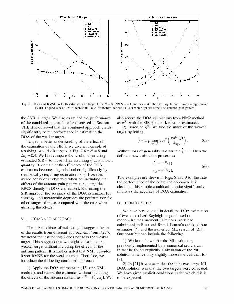
Fig. 8. Bias and RMSE in DOA estimators of target 1 for N = 8, RRCS ° = 1 and ¢´ = :4. The two targets each have average power15 dB. Legend NM1 : RRCS represents DOA estimators defined in (47) which ignore effects of antenna gain pattern.

the SNR is larger. We also examined the performanceof the combined approach to be discussed in SectionVIII. It is observed that the combined approach yieldssignificantly better performance in estimating theDOA of the weaker target.To gain a better understanding of the effect of

the estimation of the SIR °, we give an example ofresolving two 15 dB targets in Fig. 7 for N = 8 and¢´ = 0:4. We first compare the results when usingestimated SIR ° to those when assuming ° as a knownquantity. It seems that the efficiency of the DOAestimators becomes degraded rather significantly by(realistically) requiring estimation of °. However,mixed behavior is observed when not including theeffects of the antenna gain pattern (i.e., using theRRCS directly in DOA estimators). Estimating theSIR improves the accuracy of the DOA estimators forsome ´1, and meanwhile degrades the performance forother ranges of ´1, as compared with the case whenutilizing the RRCS.

VIII. COMBINED APPROACH

The mixed effects of estimating ° suggests fusionof the results from different approaches. From Fig. 7,we noted that estimating ° does not help the weakertarget. This suggests that we ought to estimate theweaker target without including the effects of theantenna pattern. It is further noted that NM1 provideslower RMSE for the weaker target. Therefore, weintroduce the following combined approach.

1) Apply the DOA estimator in (47) (the NM1method), and record the estimates without includingthe effects of the antenna pattern as ´(0) = [ ˆ1, ˆ2]. We

also record the DOA estimations from NM2 methodas ´(1) with the SIR ° either known or estimated.2) Based on ´(0), we find the index of the weaker

target by letting

j = arg minj2f1,2g

cos2µ¼´(0)(j)4´bw

¶: (65)

Without loss of generality, we assume j = 1. Then wedefine a new estimation process as

ˆ1 = ´(0)(1)

ˆ2 = ´(1)(2):

(66)

Two examples are shown in Figs. 8 and 9 to illustratethe performance of the combined approach. It isclear that this simple combination quite significantlyimproves the accuracy of DOA estimation.

IX. CONCLUSIONS

We have here studied in detail the DOA estimationof two unresolved Rayleigh targets based onmonopulse measurements. Previous work hadculminated in Blair and Brandt-Pearce’s quick ad-hocestimator [7], and the numerical ML search of [21].Our contributions include the following.

1) We have shown that the ML estimator,previously implemented by a numerical search, canin fact be found explicitly. Calculation of the MLsolution is hence only slightly more involved than for[7].2) In [21] it was seen that the joint two-target ML

DOA solution was that the two targets were colocated.We have given explicit conditions under which this isto be expected.


Fig. 9. Bias and RMSE in DOA estimators of target 1 for N = 8, RRCS ° = 0:5 and ¢´ = :4. Here target 1 is around 16 dB and target2 is 13 dB.

3) The familiar monopulse ratio for DOAestimation of a single target becomes a clear candidatewhen the effect of thermal noise is removed. We haveapplied the same philosophy here to the two-targetproblem, and have developed the “noiseless-model”joint DOA estimator NM1. NM1 can be improved byestimating the effect of thermal noise, and we alsopresent a small modification on it, NM2.4) We have provided an alternative development to

NM2 in Appendix C. This development is statisticallyrigorous, and the NM2 results give theoretical supportnot only to NM2 and NM1, but also to Blair andBrandt-Pearce’s quick ad-hoc estimator.5) We have shown via simulation that all four

of the above DOA estimators provide, in aggregate,similar performance.6) We have developed an EM estimator for joint

DOA estimation. In fact, there are three variants ofEM: with known relative SNR, with the relative SNRestimated from the data without prior information(EM2), and with the relative SNR estimated fromthe data with prior information both of the relativeRCS and the beam-pattern (EM3). Note that anyoff-boresight target will have its sum-channel returnstrength attenuated by the beam pattern (we generallyassume a raised-cosine shape in simulation) and theamount of the off-boresight angle.7) All three of the EM procedures exhibit

performance similar to each other and to the previous4 explicit DOA estimators.a) This implies that it is unnecessary to include the

beam-pattern effects in DOA estimation (a welcomedevelopment!), and that it is quite sufficient to suggestthe simple “two-stage” expedient (adopted by mostof the DOA estimators presented) of DOA estimationignoring the beam pattern, followed by reestimation of

the effective SNR from the beam pattern, followed bya second DOA estimation step.b) There is probably little reason to use EM for

this problem. However, the EM formalism developedhere is flexible, and may in the future be extended toinclude other effects.8) The explicit DOA estimators have comparable

numerical load, and provide similar aggregateperformance. However, this is by no means uniform,and it has been observed that some estimatorsare strongest exactly where others are weak. Thiscomplementarity has encouraged us to suggest asimple “combined” (fused) approach based on the NMmethods. The performance of the combined approachis highly encouraging.

APPENDIX A. A NOTE ON EXCHANGEABILITY OFTHE ESTIMATES

In all modes of analysis we have specified that´1 ¸ ´2. This includes the new estimators that we havederived here, but also the explicit ML estimator(s) (see[21]), and also the Blair and Brandt-Pearce’s modifiedmonopulse method [7]. At first this assumption seemsinnocuous: it merely excludes the mirror-imagesolution where ´2 ¸ ´1. But there is a subtlety.To understand, let us turn to the explicit ML

estimator–although it must be understood that theconclusions apply to all, and the ML is chosen fordiscussion simply because its message is explicit.First, suppose that ° = 1; that is, that both targets havethe same strength. Then it is easy to show that ( ˆ1, ˆ2)and ( ˆ2, ˆ1) are both ML pairs.But let us now assume that ° > 1. Then according

to Section IIIB we first solve a correspondingequal-SNR problem and then convert that to the true


model. The conversion is done according to (37),and it is easily seen that we have, in general, twodifferent ML pairs ( â1, ˆ

a2) and ( ˆ

b1 , ˆ

b2)6= ( â2, â1). Our

insistence that ´1 ¸ ´2 has obscured this; in a sense, toonly admit solutions in which ˆ1 ¸ ˆ2 is tantamount tosaying that the strong target is always on the right. Wehave the following.

1) When ° = 1 (equal SNR targets) the issueis moot, since the solutions are exchangeable. Thetwo electronic DOAs ( ˆ1 and ˆ2) are reported to thesystem without labeling, and presumably a trackingalgorithm associates each datum to its progenitor.2) A solution would therefore seem to be to

optimize assuming ° = 1, and ignore the issue.However, the estimated DOAs that arise are lessaccurate than if the true SNR were chosen.3) If there were prior information that ´1 ¸ ´2

(or vice versa) then the exchangeability issue doesnot arise. This is possible. A tracker may knowthat the higher SNR target is on the right, but suchinformation may not exist or may be unreliable.4) It is possible to report both ( â1, ˆ

a2) and ( ˆ

b1 , ˆ

b2)

to the tracker as pairs. The true solution couldtherefore be judged from within the tracking algorithmaccording to data association.7 We are not aware of atracking architecture that presently is capable of usingsuch measurement pairs, however.

Often the pairs ( ˆb1 , ˆb2) and ( ˆ

a2, ˆ

a1) are close. However,

we note the issue here: the observations and model arenot rich enough to disambiguate.

APPENDIX B. DERIVATION OF LIKELIHOODFUNCTION (40) AND NM1 DOA ESTIMATOR (47)

Here we work on the model (39), assuming theobservations are noiseless. Due to the independence ofthe in-phase and quadrature channels, we have

p(sI ,sQ,dI ,dQ j ´1,´2) = p(sI ,dI j ´1,´2)p(sQ,dQ j ´1,´2):Symmetry reveals that the observation pair (sI ,dI)follows the same conditional distribution as (sQ,dQ).We can describe the in-phase observations in a vectorform, µ

sI

dI

¶=µ1 1

´1 ´2

¶µx1

x2

¶= Bx (67)

and note that the covariance matrix of x is

§x =µa21 0

0 a22

¶:

7For example, the normalized innovations [2] (notionally, distance)for the association (¿1$ â

2,¿2$ â1) may be less than any of

f(¿1$ â1,¿2$ â

2), (¿1$ ˆb1 ,¿2$ ˆb

2 ), (¿1$ ˆb2 ,¿2$ ˆb

1 )g, where¿i$ ˆ

j indicates that target i comes from measurement j. Thenthe pair ( â1, ˆ

a2) is chosen, and one of its two possible associations

chosen.

Then it can be shown thatµsI

dI

¶j ´1,´2 »N(0,C), with

C= B§xBT =

µa21 + a

22 a21´1 + a

22´2

a21´1 + a22´2 a21´

21 + a

22´22

¶ (68)

according to the properties of the Gaussiandistribution [9]. Applying this vector-valued Gaussiandistribution and taking the logarithm, we have

¢(´1,´2) = logp(sI ,sQ,dI ,dQ j ´1,´2)= logp(sI ,dI j ´1,´2)+ logp(sQ,dQ j ´1,´2)

=¡ log(j2¼Cj)¡ 12 (sI dI)C

¡1µsI

dI

¶¡ 1

2 (sQ dQ)C¡1µsQ

dQ

¶=¡2log(2¼)¡ log(r)¡ a

21g1 + a

22g2

2r(69)

with j:j meaning the determinant of a matrix, and theterms

r = jCj= a21a22(´1¡ ´2)2

g1 = [(´1sI ¡ dI)2 + (´1sQ¡ dQ)2]g2 = [(´2sI ¡ dI)2 + (´2sQ¡ dQ)2]:

For N independent subpulses, we have the overalllog-likelihood function

LL =NXk=1

¢k(´1,´2)

=NXk=1

½¡2log(2¼)¡ log(r)¡ a

21g1(k) + a

22g2(k)

2r

¾(70)

with g1(k) and g2(k) calculated based on theobservations of the kth subpulse. We want to simplifythe DOA estimation by utilizing relationships betweenunknowns. Defining A0, A1, and A2 as in (19), wederive

@LL@a21

=NXk=1

½¡ 1a21+(sI(k)´2¡dI(k))2 + (sQ(k)´2¡ dQ(k))2

2(´1¡ ´2)2a41

¾= 0, thus (71)

a21 =A2´

22 ¡ 2A1´2 +A02N(´1¡ ´2)2

:

Similarly by solving @LL=@a22 = 0, we obtain

a22 =A2´

21 ¡ 2A1´1 +A02N(´1¡ ´2)2

: (72)


Therefore, using the definition of the RRCS, we findthe following relationship

° =a22a21=A2´

21 ¡ 2A1´1 +A0

A2´22 ¡ 2A1´2 +A0

: (73)

We further examine the partial derivatives

@LL@´1

=NXk=1

½¡ 2´1¡ ´2

¡ sI(k)(sI(k)´1¡ dI(k)) + sQ(k)(sQ(k)´1¡dQ(k))a22(´1¡ ´2)2

+a21g1(k)+ a

22g2(k)

r(´1¡ ´2)¾

@LL@´2

=NXk=1

½¡ 2´2¡ ´1

¡ sI(k)(sI(k)´2¡ dI(k)) + sQ(k)(sQ(k)´2¡dQ(k))a21(´1¡ ´2)2

+a21g1(k)+ a

22g2(k)

r(´2¡ ´1)¾:

These imply

@LL@´1

+@LL@´2

=¡ A2´1¡A1a22(´1¡ ´2)2

¡ A2´2¡A1a21(´1¡ ´2)2

= 0

(74)

or

´1 =A1A2

µ1+

a22a21

¶¡ a

22

a21´2: (75)

Now the relationships expressed in (75) and (73)can be jointly solved to estimate the DOAs of twounresolved targets, giving

°A2´22 ¡ 2°A1´2¡A0 +A21(1+ °)=A2 = 0: (76)

The constraint ´1¡ ´2 > 0 yields the unique choice ofthe solutions of this second order polynomial functionas

ˆ1 =A1 +

q(A2A0¡A21)°A2

ˆ2 =A1¡

q(A2A0¡A21)=°A2

:

(77)

Therefore, we have the DOA estimator in (47).

APPENDIX C. ALTERNATIVE DERIVATION OF NM2DOA ESTIMATOR (49)

We work on the observation model (1), where thenoises are included. Due to the independence of thein-phase and quadrature channels, it is easy to showthat

°(´1,´2) = p(sI ,sQ,dI ,dQ j ´1,´2)= p(sI ,dI j ´1,´2)p(sQ,dQ j ´1,´2): (78)

By restating model (1) in vector notation we get

µsI

dI

¶=µ1 1 1 0

´1 ´2 0 1

¶0BBB@x1

x2

nsI

ndI

1CCCA=Ab: (79)

Recall that b»N(0,§) with § = diag(a21,a22,¾2s ,¾2d)since components of b are statistically independent. Itis straightforward to show that (17) and (18) describethe joint probability density.Often only the RRCS is known, while the absolute

RCS’s a21 and a22 are unknown and need to be

estimated based on observations. To estimate theDOAs ´1 and ´2, our approach is to estimate thecovariance matrix R and then match the estimatedR to the ideal covariance matrix in (18). For Nindependent subpulses the elements of the covariancematrix can be estimated as

r11 = E(s2I ) = E(s

2Q)»= 12N

NXk=1

fsI(k)2 + sQ(k)2g=A22N

r12 = r21 = E(sIdI) = E(sQdQ)(80)

»= 12N

NXk=1

fsI(k)dI(k) + sQ(k)dQ(k)g=A12N

r22 = E(d2I ) = E(d

2Q)»= 12N

NXk=1

fdI(k)2 + dQ(k)2g=A02N

with rij denoting the ith row and jth column elementof the matrix R, and the operation »= means that theleft term is estimated by the expression on the right.Recalling that the RRCS ° is known, and now alsomatching each element of the estimated R to the onedefined in (18), we have four equations.Further considering the constraint ´1¡ ´2 > 0

to ensure a unique solution, we can show thatthese four equations are solvable to the fourunknowns as

a21 =A2¡ 2N¾2s2N(1+ °)

=A2

2N(1+ °)

a22 =°A2

2N(1+ °)

ˆ1 =A1 +

q(A2A0¡ A21)°A2

ˆ2 =A1¡

q(A2A0¡ A21)=°A2

(81)


with A0, A1, and A2 expressed in (48). We thushave an alternative derivation of the modified DOAestimator (49), one that is perhaps more rigorous thanthat presented earlier.

APPENDIX D. DERIVATION OF EM METHOD

Based on the likelihood function of the completedata f(x j µ) defined as in (52), and recalling theconditional pdf

f(h j r,µ[i]) = f(r j h,µ[i])f(h j µ[i])

f(r j µ[i]) =f(x j µ[i])f(r j µ[i])

we now calculate the Q function

Q(µ j µ[i]) = Eflogf(x j µ) j r,µ[i]g

=

Z¢ ¢ ¢Zh

f(h j r,µ[i]) logf(x j µ)dh

=1

f(r j µ[i])

Zh

f(x j µ[i]) logf(x j µ)dh

=exp(g1(µ

[i]))f(r j µ[i])

Zh

(g1(µ) + g2(h,µ))exp(g2(h,µ[i]))dh:

(82)From the definitions in (53), it is clear thatZ

hg1(µ)exp(g2(h,µ

[i]))dh= g1(µ): (83)

Also, by using

EfAxg=A¹, EfxTAxg= Tr(AR)in which Tr denotes the trace operation, x isa Gaussian random vector with mean ¹ andautocovariance matrix R, and for which A is arbitrarysymmetric matrix [1]. We have

log(N(hk; rk(µ),Rh(µ)) =¡0:5log(j2¼Rh(µ)j)¡ 0:5(hk ¡ rk(µ))TR¡1h (µ)(hk ¡ rk(µ))

andZh

g2(h,µ)exp(g2(h,µ[i]))dh

=NXk=1

Zhk

log(N(hk; rk(µ),Rh(µ))N(hk; rk(µ[i]),Rh(µ

[i])dhk

=¡N2log(j2¼Rh(µ)j)¡

12Tr(R¡1h (µ)Rh(µ

[i]))

¡ 12

NXk=1

(rk(µ[i])¡ rk(µ))TR¡1h (µ)(rk(µ[i])¡ rk(µ)):

(84)

Therefore, combining (83) with (84) together leads to

Q(µ j µ[i]) = exp(g1(µ[i]))

f(r j µ[i])

"g11 +

NXk=1

dk(µ,µ[i])

#(85)

with g11 and dk as defined in (55). This completes theexpression of the expectation Q(µ j µ[i]).In the M-step, we need to consider the

maximization problem

µ[i+1] = argmaxµQ(µ j µ[i]) = argmax

µ

NXk=1

dk(µ,µ[i])

(86)

since exp(g1(µ[i])), f(r j µ[i]) and g11 are not functions

of µ. We first note that

@R¡1h (µ)@´1

=

0BBBBBBBB@

2´1¾2d

´2¾2d

0 0

´2¾2d

0 0 0

0 0 2´1¾2d

´2¾2d

0 0´2¾2d

0

1CCCCCCCCA

@R¡1h (µ)@´2

=

0BBBBBBBB@

0´1¾2d

0 0

´1¾2d

2´2¾2d

0 0

0 0 0´1¾2d

0 0´2¾2d

2´2¾2d

1CCCCCCCCA

@A(µ)T

@´1=

0BBB@0 1 0 0

0 0 0 0

0 0 0 1

0 0 0 0

1CCCA

@A(µ)T

@´2=

0BBB@0 0 0 0

0 1 0 0

0 0 0 0

0 0 0 1

1CCCA

Rss(µ[i]) =

1jR¡1ss (µ[i])j

0BB@´22¾2d+1¾2s+1a22

¡µ´1´2¾2d

+1¾2s

¶¡µ´1´2¾2d

+1¾2s

¶´21¾2d+1¾2s+1a21

1CCA

=

µc11(µ

[i]) c12(µ[i])

c12(µ[i]) c22(µ

[i])

¶:

We also note that

R¡1n rk =·sI(k)¾2s

,dI(k)¾2d

,sQ(k)

¾2s,dQ(k)

¾2d

¸and further for simplicity define rk(µ

[i]) =[r[i]k (1), : : : , r

[i]k (4)]. We thus have the partial differential


equation

@dk(µ,µ[i])

@´1

=¡12rk(µ

[i])T@R¡1h (µ)@´1

rk(µ[i])

+ rk(µ[i])T

@A(µ)T

@´1R¡1n rk ¡

12Tr

Ã@R¡1h (µ)@´1

Rh(µ[i])

!

=¡ (r[i]k (1)

2 + r[i]k (3)2)´1 + (r

[i]k (1)r

[i]k (2)+ r

[i]k (3)r

[i]k (4))´2

¾2d

+r[i]k (1)dI(k)+ r

[i]k (3)dQ(k)

¾2d¡ 2(c11(µ

[i])´1 + c12(µ[i])´2)

¾2d:

(87)

Therefore, equating the overall differential result tozero yields

NXk=1

@dk(µ,µ[i])

@´1= e01 + e11´1 + e12´2 = 0: (88)

Similarly, differentiating with respect to ´2 andequating the result to zero yields

NXk=1

@dk(µ,µ[i])

@´2= e02 + e12´1 + e22´2 = 0 (89)

in which all the e-terms are expressed as in (57).Therefore, the estimate of DOAs should be updatedby solvingµ

e11 e12

e12 e22

¶Ã´[i+1]1

´[i+1]2

!=¡

µe01

e02

¶: (90)

Assuming the inverse matrix exists, this results in thesolution (56).To take the antenna gain into account, we also

need to estimate a21 and a22. In the first model, we

consider µ = f´1,´2,a21,a22g. In the M-step, as shownin (88) and (89), @Q(µ j µ[i])=@´1 and @Q(µ j µ[i])=@´2are not functions of a21 and a

22. The estimate of DOAs

should consequently still be updated as in (90). Wefurther note that

@g11@a21

=¡Na¡21 ,@A(µ)T

@a21= 0

@R¡1h (µ)@a21

=

0BBB@¡a¡41 0 0 0

0 0 0 0

0 0 ¡a¡41 0

0 0 0 0

1CCCA@g11@a22

=¡Na¡22 ,@A(µ)T

@a22= 0

@R¡1h (µ)@a22

=

0BBB@0 0 0 0

0 ¡a¡42 0 0

0 0 0 0

0 0 0 ¡a¡42

1CCCA :Therefore, equating the overall differential result tozero yields

@Q(µ j µ[i])@a21

=¡Na¡21 + a¡41

NXk=1

£³12 (r

[i]k (1)

2 + r[i]k (3)2)+ c11(µ

[i])´= 0

(91)@Q(µ j µ[i])

@a22=¡Na¡22 + a¡42

NXk=1

£³12 (r

[i]k (2)

2 + r[i]k (4)2)+ c22(µ

[i])´= 0:

Thus the solution (61) is obtained.In the second model, we assume that a22 = °a

21,

and we consider µ = f´1,´2,a21g. Similar to the abovemodel, in the M-step, the estimate of DOAs shouldstill be updated as in (90). We further note that

@g11@a21

=¡2Na¡21 ,@A(µ)T

@a21= 0

@R¡1h (µ)@a21

=

0BBBBBBBB@

¡a¡41 0 0 0

0¡a¡41°

0 0

0 0 ¡a¡41 0

0 0 0¡a¡41°

1CCCCCCCCA:

Therefore, equating the overall differential result withrespect to a21 to zero gives

@Q(µ j µ[i])@a21

=¡2Na¡21 + a¡41

NXk=1

£Ã12(r[i]k (1)

2 + r[i]k (3)2)+

12°(r[i]k (2)

2 + r[i]k (4)2)

+ c11(µ[i]) +

1°c22(µ

[i])

!:

Thus the solution (63) is obtained.

APPENDIX E. DERIVATION OF ML ESTIMATE OF a21IN STEP 2

Recall that a22 = °a21 is assumed in this section.

Working on the observation model (1), due toindependence of subpulses, and referring to (17), we


can show that

LL = log(p(r j ´1,´2,a21)) =¡N log(j2¼Rj)

¡ 12

NXk=1

Ã(sI(k) dI(k))R

¡1µsI(k)

dI(k)

¶

+(sQ(k) dQ(k))R¡1µsQ(k)

dQ(k)

¶!

=¡N log(j2¼Rj)¡ 12jRj (n1a

21 + n0) (92)

in which A0, A1, and A2 are defined as in (19), and

n1 = A2(´21 + °´

22)¡ 2A1(´1 + °´2)+A0(1+ °)

n0 = A2¾2d +A0¾

2s :

We also have

jRj= °(´1¡ ´2)2a41 + [(1+ °)¾2d +(´21 + °´22)¾2s ]a21 +¾2s ¾2d=m2a

41 +m1a

21 +m0:

Accordingly, setting the derivative @LL=@a21 = 0 givesthe following cubic polynomial

¡ 2Nm22a61 +³n1m2

2¡ 3Nm1m2

´a41

+ (m2n0¡Nm21¡ 2Nm0m2)a21+³m1n0

2¡Nm0m1¡

m0n12

´= 0: (93)

Therefore, the ML solution for a21 can be easilyobtained by solving the above polynomial and pickingup the real positive solution. Further, from this, theestimate of a22 is correspondingly updated by a

22 = °a

21.

REFERENCES

[1] Bar-Shalom, Y., Li, X., and Kirubarajan, T. (1999)Estimation and Tracking: Principles Techniques andSoftware.Storrs, CT: YBS Publishers, 1999.

[2] Bar-Shalom, Y., and Li, X. (1995)Multitarget-Multisensor Tracking: Principles andTechniques.Storrs, CT: YBS Publishers, 1995.

[3] Barton, D. (1974)Low-angle radar tracking.Proceedings of the IEEE, (June 1974), 687—804.

[4] Berkowitz, R., and Sherman, S. (1971)Information derivable from monopulse radarmeasurements of two unresolved targets.IEEE Transactions on Aerospace and Electronic Systems,AES-7 (Sept. 1971), 1011—1013.

[5] Blair, W., and Brandt-Pierce, M. (1998)Statistical description of monopulse parameters fortracking Rayleigh targets.IEEE Transactions on Aerospace and Electronic Systems,(Apr. 1998), 597—611.

[6] Blair, W., Watson, G., Kirubarajan, T., and Bar-Shalom, Y.(1998)Benchmark for radar allocation and tracking in ECM.IEEE Transactions on Aerospace and Electronic Systems,34, 4 (Oct. 1998), 1097—1114.

[7] Blair, W., and Brandt-Pearce, M. (2001)Monopulse DOA estimation of two unresolved Rayleightargets.IEEE Transactions on Aerospace and Electronic Systems,37, 2 (Apr. 2001).

[8] Dempster, A., Laird, N., and Rubin, D. (1977)Maximum likelihood from incomplete data via the EMalgorithm.Journal of the Royal Statistical Society, Series B, 39, 1(1977), 1—38.

[9] Haykin, S. (1996)Adaptive Filter Theory (3rd ed.).Englewood Cliffs, NJ: Prentice-Hall, 1996.

[10] Haykin, S., Litva, J., and Shepherd, T. (1993)Radar Array Processing.New York: Springer-Verlag, 1993.

[11] Hofstetter, E., and DeLong, D. (1969)Detection and parameter estimation in anamplitude-comparison monopulse radar.IEEE Transactions on Aerospace and Electronic Systems,AES-5 (Jan. 1969).

[12] Moon, T. (1996)The expectation-maximization algorithm.IEEE Signal Processing Magazine, (Nov. 1996), 47—60.

[13] Mosca, E. (1969)Angle estimation in amplitude comparison monopulsesystem.IEEE Transactions Aerospace and Electronic Systems,AES-5, 2 (Mar. 1969), 205—212.

[14] Nickel, U. (1993)Monopulse estimation with adaptive arrays.IEE Proceedings, Pt. F, 140, 5 (1993), 303—308.

[15] Nickel, U. (1999)Performance of corrected adaptive monopulse estimation.IEE Proceedings, Pt. F, (Feb. 1999).

[16] Neilsen, R. (2001)Accuracy of angle estimation with monopulse processingof two beams.IEEE Transactions on Aerospace and Electronic Systems,(Oct. 2001).

[17] Peebles, P., and Berkowitz, R. (1968)Multiple-target monopulse radar processing techniques.IEEE Transactions on Aerospace and Electronic Systems,AES-4 (Nov. 1968), 845—854.

[18] Sharenson, S. (1962)Angle estimation accuracy with a monopulse radar insearch mode.IRE Transactions on Aerospace and Electronic Systems,(Sept. 1962).

[19] Sherman, S. (1984)Monopulse Principles and Techniques.Boston: Artech House, 1984.

[20] Sherman, S. (1971)Complex indicated angles applied to unresolved radartargets and multipath.IEEE Transactions on Aerospace and Electronic Systems,AES-7, 1 (Jan. 1971), 160—170.

[21] Sinha, A., Kirubarajan, T., and Bar-Shalom, Y. (2002)Maximum likelihood angle extractor for two closelyspaced targets.IEEE Transactions on Aerospace and Electronic Systems,38, 1 (Jan. 2002), 183—203.

[22] Slocumb, B., and Blair, W. D. (2002)EM-based measurement fusion for HRR radar centroidprocessing.In Proceedings of the SPIE Conference on Signal and DataProcessing of Small Targets, Orlando, FL, Apr. 2002.


[23] Tong, L., and Perreau, S. (1998)Multichannel blind identification: From subspace tomaximum likelihood methods.Proceedings of the IEEE, 86, 10 (1998), 1951—1967.

[24] Valeri, M., Barbarossa, S., Farina, A., and Timmoneri, L.(1996)Monopulse estimation of target DOA in external noisefields with adaptive arrays.Presented at the IEEE International Symposium onPhased Array Systems and Technology, Oct. 1996.

Zhen Wang received the B.Sc. degree from Tsinghua University, China, in1996, and the M.Sc. and Ph.D. degrees (with the Outstanding EngineeringDoctoral Student Award) from the University of Connecticut in 2000 and 2002,respectively, all in electrical engineering. She has been a research associate ofthe Electrical and Computer Engineering Department and Institute for SystemsResearch at the University of Maryland, College Park. Since August 1, 2004,she has been with the Department of Electrical and Computer Engineering at theUniversity of British Columbia, Canada, as an assistant professor. Her researchinterests are in the broad areas of statistical signal processing, informationsecurity, biomedical imaging, genomic, and wireless communications.

Abhijit Sinha has received his B.S. degree in physics from the University ofCalcutta in 1994. He received his M.S. degree in electrical communicationengineering from Indian Institute of Science in 1998. He is currently workingtowards his Ph.D. degree in electrical and computer engineering at University ofConnecticut. His research interests include estimation, detection, and tracking.

Peter K. Willett (S’83–M’86–SM’97) was born in Toronto, Ontario, Canada.He received the B.Sc. degree in engineering science from the University ofToronto in 1982. He received the M.E. and M.S. degrees in 1983 and 1984,respectively, and the Ph.D. degree in 1986, all in electrical engineering, fromPrinceton University, Princeton, NJ.He is professor with the University of Connecticut, Storrs, where he has been

since 1986. His interests are generally in detection theory, target tracking, andsignal processing. Dr. Willett is an associate editor for the IEEE Transactionson Sytems, Man, and Cybernetics and the IEEE Transactions on Aerospace andElectronic Systems.

[25] Willett, P., Blair, W. D., and Bar-Shalom, Y. (2003)On the correlation between horizontal and verticalmonopulse measurements.IEEE Transactions on Aerospace and Electronic Systems,39, 2 (Apr. 2003), 533—549.


Yaakov Bar-Shalom (S’63–M’66–SM’80–F’84) was born on May 11, 1941.He received the B.S. and M.S. degrees from the Technion, Israel Institute ofTechnology, in 1963 and 1967 and the Ph.D. degree from Princeton University,Princeton, NJ, in 1970, all in electrical engineering.From 1970 to 1976 he was with Systems Control, Inc., Palo Alto, CA.

Currently he is Board of Trustees Distinguished Professor in the Dept. ofElectrical and Computer Engineering and director of the ESP Lab (Estimationand Signal Processing) at the University of Connecticut. His research interests arein estimation theory and stochastic adaptive control and he has published over300 papers and book chapters in these areas. In view of the causality principlebetween the given name of a person (in this case, “(he) will track,” in the modernversion of the original language of the Bible) and the profession of this person,his interests have focused on tracking.He coauthored the monograph Tracking and Data Association (Academic

Press, 1988), the graduate text Estimation with Applications to Tracking andNavigation (Wiley, 2001), the text Multitarget-Multisensor Tracking: Principles andTechniques (YBS Publishing, 1995), and edited the books Multitarget-MultisensorTracking: Applications and Advances (Artech House, Vol. I 1990; Vol. II 1992,Vol. III 2000). He has been elected Fellow of IEEE for “contributions to thetheory of stochastic systems and of multitarget tracking.” He has been consultingto numerous companies, and originated the series of Multitarget-MultisensorTracking short courses offered via UCLA Extension, at Government Laboratories,private companies, and overseas. He has also developed the commerciallyavailable interactive software packages MULTIDAT TM for automatic trackformation and tracking of maneuvering or splitting targets in clutter, VARDATTM for data association from multiple sensors, BEARDAT TM for targetlocalization from bearing and frequency measurements in clutter, IMDAT TM forimage segmentation and target centroid tracking and FUSEDAT TM for fusionof possibly heterogeneous multisensor data for tracking. During 1976 and 1977he served as associate editor of the IEEE Transactions on Automatic Control andfrom 1978 to 1981 as associate editor of Automatica. He was program chairmanof the 1982 American Control Conference, general chairman of the 1985 ACC,and cochairman of the 1989 IEEE International Conference on Control andApplications. During 1983—1987 he served as chairman of the ConferenceActivities Board of the IEEE Control Systems Society and during 1987—1989was a member of the Board of Governors of the IEEE CSS. Currently he is amember of the Board of Directors of the International Society of InformationFusion and served as its Y2K and Y2K2 President. In 1987 he received the IEEECSS distinguished Member Award. Since 1995 he is a distinguished lecturer ofthe IEEE AESS. He is corecipient of the M. Barry Carlton Awards for the bestpaper in the IEEE Transactions on Aerospace and Electronic Systems in 1995 and2000, and received the 1998 University of Connecticut AAUP Excellence Awardfor Research and the 2002 J. Mignona Data Fusion Award from the DoD JDLData Fusion Group.


angle estimation for two unresolved targets with …zjanew/journal/zjw_aes_aemonradar_23.pdf ·...

Documents