andrew d. ker 16 lectures, michaelmas term 2010 mathematics andrew d. ker 16 lectures, michaelmas...
TRANSCRIPT
Discrete Mathematics
Andrew D. Ker
16 Lectures, Michaelmas Term 2010
Oxford University Computing Laboratory

ii
Contents
Introduction To The Lecture Notes vii
1 Sets 1
1.1 Defining Sets . . . . . . . . . . . . . . . . . . . . . . . . . . . 1
1.2 Comparing Sets and Writing Proofs . . . . . . . . . . . . . . 4
1.3 Unions, Intersections, and Algebraic Laws . . . . . . . . . . . 5
1.4 Complements, Symmetric Difference, Laws . . . . . . . . . . . 8
1.5 Products and Power Sets . . . . . . . . . . . . . . . . . . . . 10
1.6 Cardinality . . . . . . . . . . . . . . . . . . . . . . . . . . . . 12
1.7 Interesting Diversion: Bags . . . . . . . . . . . . . . . . . . . 12
Practice Questions . . . . . . . . . . . . . . . . . . . . . . . . . . . 14
2 Functions 17
2.1 Intervals . . . . . . . . . . . . . . . . . . . . . . . . . . . . . . 17
2.2 Definition of Functions . . . . . . . . . . . . . . . . . . . . . . 18
2.3 Properties of Functions . . . . . . . . . . . . . . . . . . . . . 20
2.4 Contrapositive and Proof by Contradiction . . . . . . . . . . 21
2.5 Composition and Inverse . . . . . . . . . . . . . . . . . . . . . 24
2.6 Interesting Diversion: Binary Operators . . . . . . . . . . . . 26
Practice Questions . . . . . . . . . . . . . . . . . . . . . . . . . . . 28
iii
iv CONTENTS
3 Counting 31
3.1 Laws of Sum and Product . . . . . . . . . . . . . . . . . . . . 32
3.2 The Technique of Double Counting . . . . . . . . . . . . . . . 34
3.3 The Inclusion-Exclusion Principle . . . . . . . . . . . . . . . . 38
3.4 Ceiling and Floor Functions . . . . . . . . . . . . . . . . . . . 40
3.5 Interesting Diversion: Multinomial Coefficients . . . . . . . . 41
Practice Questions . . . . . . . . . . . . . . . . . . . . . . . . . . . 43
4 Relations 45
4.1 Definition . . . . . . . . . . . . . . . . . . . . . . . . . . . . . 45
4.2 Properties of Relations . . . . . . . . . . . . . . . . . . . . . . 46
4.3 Equivalence Relations . . . . . . . . . . . . . . . . . . . . . . 48
4.4 Operations on Relations . . . . . . . . . . . . . . . . . . . . . 50
4.5 Drawing Relations . . . . . . . . . . . . . . . . . . . . . . . . 52
4.6 Interesting Diversion: Counting Relations . . . . . . . . . . . 53
Practice Questions . . . . . . . . . . . . . . . . . . . . . . . . . . . 55
5 Sequences 57
5.1 Definition . . . . . . . . . . . . . . . . . . . . . . . . . . . . . 57
5.2 Proof by Induction . . . . . . . . . . . . . . . . . . . . . . . . 59
5.3 Sigma Notation and Sums of Sequences . . . . . . . . . . . . 61
5.4 Sequences Associated with Counting . . . . . . . . . . . . . . 62
5.5 Solving Linear Recurrence Relations . . . . . . . . . . . . . . 65
Practice Questions . . . . . . . . . . . . . . . . . . . . . . . . . . . 68
6 Modular Arithmetic 71
6.1 Definitions . . . . . . . . . . . . . . . . . . . . . . . . . . . . . 71
6.2 Exponentiation . . . . . . . . . . . . . . . . . . . . . . . . . . 73
6.3 mod and div . . . . . . . . . . . . . . . . . . . . . . . . . . . 74
6.4 Euclid’s Algorithm and Multiplicative Inverses . . . . . . . . 75
CONTENTS v
6.5 The Pigeonhole Principle . . . . . . . . . . . . . . . . . . . . 77
6.6 Modular Square Roots of -1 . . . . . . . . . . . . . . . . . . . 80
Practice Questions . . . . . . . . . . . . . . . . . . . . . . . . . . . 82
7 Asymptotic Notation 85
7.1 Big-O Notation . . . . . . . . . . . . . . . . . . . . . . . . . . 85
7.2 Proving Sentences of the form ∃x.∀y.P . . . . . . . . . . . . . 87
7.3 Tail Behaviour . . . . . . . . . . . . . . . . . . . . . . . . . . 89
7.4 Asymptotics of n! . . . . . . . . . . . . . . . . . . . . . . . . . 89
7.5 Asymptotic Behaviour of Recurrence Relations . . . . . . . . 91
7.6 Recurrences of Divide-and-Conquer Type . . . . . . . . . . . 92
Practice Questions . . . . . . . . . . . . . . . . . . . . . . . . . . . 95
8 Orders 97
8.1 Definitions . . . . . . . . . . . . . . . . . . . . . . . . . . . . . 97
8.2 Orders on Cartesian Products . . . . . . . . . . . . . . . . . . 99
8.3 Drawing Orders . . . . . . . . . . . . . . . . . . . . . . . . . . 101
8.4 Upper and Lower Bounds . . . . . . . . . . . . . . . . . . . . 103
8.5 Proving Sentences of the form ∀x.∃y.P . . . . . . . . . . . . . 105
8.6 Interesting Diversion: Order Isomorphisms . . . . . . . . . . . 107
Practice Questions . . . . . . . . . . . . . . . . . . . . . . . . . . . 109
Index 111

vi CONTENTS
Introduction To The Lecture
Notes
Course
The Discrete Mathematics course is compulsory for first-year undergrad-uates in Computer Science. There are 16 lectures, supported by tutorialsarranged by college tutors.
Prerequisites
None.
Syllabus
Sets: union, intersection, difference, power set, algebraic laws. Functions:injectivity & surjectivity, composition & inverse. Relations, equivalence re-lations, and partitions; relational composition & converse, transitive closure;orders, least upper and greatest lower bounds. Combinatorial algebra: per-mutations, combinations, sums of finite sequences. Functions associatedwith combinatorial problems: ceiling, floor, factorial, combinatorial coeffi-cients. The inclusion-exclusion principle. Recurrence relations arising fromcombinatorial problems. Modular arithmetic, Euclid’s algorithm, and ap-plications.
vii
viii INTRODUCTION TO THE LECTURE NOTES
Outline of Lectures
The material is presented in eight sections, one per week. Each section isconcerned with one topic in discrete maths, and a technique for constructingmathematical proofs.
Sets: Definition of sets, subsets, some standard sets; union, intersection, rel-ative complement, symmetric difference, complement, cartesian prod-ucts, power sets; algebraic laws; cardinality of finite sets. Writingmathematical proofs, double inclusion proofs for set equality, proof bycases. Extra topic: bags.
Functions: Intervals; functions, domain and codomain, partial functions,restriction; 1-1, onto, and bijective functions; composition and inverse.Proof of the contrapositive and proof by contradiction. Extra topic:binary operators.
Counting: Counting laws of sum, subtract, product; permutations, factorialfunction, combinations, binomial coefficients; inclusion-exclusion prin-ciple, derangements; floor and ceiling functions. Proofs techniques forcounting, with many examples. Extra topic: multinomial coefficients.
Relations: Binary relations; properties of relations: reflexivity, irreflexivity,symmetry, antisymmetry, transitivity, seriality; equivalence relations,equivalence classes, and partitions; relational composition, converse,and transitive closure; graphical representation of relations. Extratopic: counting relations.
Sequences: Sequences and recurrence relations; sigma notation and partialsums of sequences; recurrence relations arising from counting prob-lems, including derangements and partitions. Proof by induction. Ex-tra topic: solving linear recurrence relations.
Modular Arithmetic: Definition of modular arithmetic via an equivalencerelation; properties of addition, multiplication, and exponentation(mod n); Euclid’s algorithm, binary mod and div functions, multi-plicative inverses (mod p). The Pigeonhole Principle and many ex-amples. Extra topic: modular square roots of −1.
ix
Asymptotic Notation: Big-O notation, tail behaviour of sequences, exam-ples drawn from running times of common algorithms. Proofs of sen-tences of the form ∃x.∀y.P , with examples of asymptotic behaviourproofs including simplified Stirling’s formula. Choosing the right in-ductive hypothesis for big-O proofs. Extra topic: solving recurrencerelations of divide-and-conquer type, up to asymptotic order.
Orders: Pre-orders, partial orders, and linear orders; chains; product andlexicographic order on cartesian products; upper and lower bounds,lub and glb. Proofs of sentences of the form ∀x.∃y.P , with examplesfrom interesting orders. Extra topic: order isomorphisms.
Reading Material
The lecture notes provide all the necessary definitions, some examples, andsome exercises. It would be a good idea, though, to buy or borrow a textbookin order to supplement and round out the material (and particularly forfinding more practice exercises). The recommended text is
K. A. Ross and C. R. B. Wright, Discrete Mathematics (FifthEdition), Prentice Hall, 2003.
This book has much to commend it, including an enormous number of exam-ples and exercises and a computer science oriented exposition. It is ratherexpensive (about £50) but there are many copies in Oxford libraries.
Three other books, which are fairly useful, are:
R. P. Grimaldi, Discrete And Combinatorial Mathematics (FifthEdition), Addison Wesley, 2003.
A bit strange, with some very advanced topics alongside the standard mate-rial. Its big advantage is comprehensive coverage of the course material andlots of good practice exercises (some difficult). Probably not worth buying,but a good book to borrow. The fifth edition is the most recent but earliereditions are equally good.
A. Chetwynd and P. Diggle, Discrete Mathematics, Arnold, 1995.
The complete opposite, this book covers the basics well. It is easy to readand worth consulting if you are struggling, but only covers the first half ofthe material in this course. Cheap.
x INTRODUCTION TO THE LECTURE NOTES
P. Grossman, Discrete Mathematics for Computing (Third Edi-tion), Palgrave MacMillan, 1995.
Moderate level with an emphasis on modern computer science applications.Covers about three quarters of our material and includes other useful chap-ters on logic (will appear in the Digital Hardware course) and graphs (willappear in Design and Analysis of Algorithms). Cheap.
Practice Questions and Tutorial Exercises
At the end of each chapter are some practice questions: usually shortand fairly simple, they are to help you test your own understanding. Briefanswers are provided on the final page of the chapter. It is recommendedto try the practice questions soon after the relevant lectures, to help youcorrect any misunderstanding quickly.
More substantial questions are set in the tutorial exercises, provided sep-arately from the notes. There will be four regular tutorial sheets, plus oneadditional sheet covering the last week’s lecture material along with generalrevision suitable for vacation work (whether to set the vacation work, or in-deed whether to follow these exercises at all, is a decision for college tutors).Model answers are provided for tutors’ use only.
It is not expected that your tutors will want to discuss the practice questionsand so it is possible to get by without doing them. However, they have beendesigned so that some of the tutorial exercises will be easier if the practicequestions have been attempted beforehand.
Course Website
Course material can be found at http://web.comlab.ox.ac.uk/teaching/
courses/discretemaths/. The lecture notes will be published about a weekafter the corresponding lectures (if you want timely notes, you will have toattend), and the tutorial exercise sheets will appear in weeks 1, 3, 5, 7 (and8 for the vacation work).
Chapter 1
Sets
Reading: Ross & Wright: 1.3, 1.4;Chetwynd & Diggle: 2.1–2.6;Grimaldi: 3.1, 3.2;Grossman: 5.1–5.3.
It is necessary to understand the concept of sets to express anything, be itmathematics or the behaviour of computer systems, formally. Furthermore,the notation of sets provides a concise way to express statements aboutcomputers. Much of the material in this chapter is probably familiar, but itis important to begin thoroughly, and sets are also a useful topic with whichto study the writing of mathematical proofs, something which will shadowthe discrete mathematics material throughout this course.
1.1 Defining Sets
Although the idea of a set as a collection of objects (in which neither ordernor duplication are significant) is simple enough, it is rather complicatedto give a formal definition from scratch. We will leave the complexitiesto mathematical philosophers and adopt a simple working definition, butyou should know that the subject called axiomatic set theory is deep anddifficult.
Definition A set is an unordered collection of distinct objects. When x
1
2 CHAPTER 1. SETS
is in the set A we say that x is an element (or member) of A and writex ∈ A. When x is not an element of A we write x /∈ A.
A set can be defined by its members, because two sets are called equal(written A = B) if they have the same members. We can therefore specifya set simply by listing its members, for example A = 1, 2, 3 which meansthe set A which has members 1, 2, 3. We can say that 1 ∈ A and 4 /∈ A.Notice the “curly brackets” (called braces) which are traditionally used todefine sets. Because neither duplicates nor order are significant, 3, 2, 1, 2represents the same set.
Sets can have infinitely many members, and it is not necessary to list themall explicitly as long it is clear what is and what is not a member. Forexample the description 1, 3, 5, 7, . . . unambiguously defines the positiveodd integers. Another way to define a set is by a set comprehension:
x | some condition on x
which denotes the set whose members are all those meeting the condition.For example,
x | x ∈ 1, 2, 3, 4, 5, 6, 7, 8, 9 and x is divisible by 4
is an over-complicated definition of the set 4, 8. The symbol “|” is some-times alternatively written as “:”; it is pronounced “such that”. (A note forthe formalist: axiomatic set theory has particular things to say about setcomprehensions – it is possible to misuse them to define things which arenot actually sets – but that will never be an issue for us in this course.)
There are two shorthands often used with set comprehensions. First, ifthe condition includes membership of a set, that part of the condition issometimes written before the bar, for example
E = n ∈ N | n/2 ∈ N
as a definition of the even integers. Second, one sometimes writes a functionbefore the bar (functions are the subject of Chapter 2): all values of thefunction, whose arguments satisfy the condition, define the set. In this waythe set E can be alternatively defined by
E = 2m | m ∈ N.
1.1. DEFINING SETS 3
A note on alphabets. There is no fundamental distinction between “element”and “set”; it is entirely possible for one set to be a member of another, forexample 1, 2, 2, 3 is a set with two members 1, 2 and 2, 3, eachof which is a set of numbers. (However, it is usually disallowed for any setto be a member of itself; this is another philosophical question we intendto avoid.) Many books adopt the practice of using lowercase Roman letterslike x and y for members of sets, and uppercase letters like A and B forsets; then they sometimes use calligraphic letters like A and B for sets ofsets. However this distinction is artificial (take for example the set 1, 1:it has one member which is a number, and another which is a set) and onequickly runs out of different alphabets if there are sets of sets of sets of...
Definition Some standard sets are
(i) ∅ = , the empty set.
(ii) N = 0, 1, 2, . . ., the natural numbers(or nonnegative integers).
(iii) N+ = 1, 2, 3, . . ., the positive integers.
(iv) Z = . . . ,−2,−1, 0, 1, 2, . . ., the integers.
(v) Zn = 0, 1, 2, . . . , n − 1, the integers modulo n(for n = 2, 3, 4, . . .).
(vi) Q, =
nd
∣
∣ n ∈ Z and d ∈ N+
, the rational numbers.
(vii) R, the real numbers.
It is unambiguous to write Z+ instead of N+, but beware! Some people writeN for the set of positive integers and something like N0 for what we havecalled N. And some write P for the set of positive integers, while others usethe same symbol for the set of prime numbers. It is truly unfortunate thatthere is no agreement on such basic terminology. The definitions we use areprobably the most common but it is important to check which version isbeing used whenever you consult a textbook.
Finally, note the distinction between and ; the first is an empty setwith no elements, whereas the second is a set with one element (and thiselement happens to be another set).
4 CHAPTER 1. SETS
1.2 Comparing Sets and Writing Proofs
There are ways to compare sets. We have already seen the first of thefollowing:
Definition When sets A and B have exactly the same members we writeA = B.
When all the elements of A are also members of B we say that A is a subsetof B, and write A ⊆ B. Two alternative ways of saying the same thing arethat A is included in B or that B is a superset of A, written B ⊇ A.
When A ⊆ B and A 6= B we say that A is a proper subset of B, writtenA ⊂ B or B ⊃ A. (This means that all members of A are also members ofB, and further that some members of B are not members of A.)
Beware! Some people write A ⊂ B to mean that A is a subset of B, and usethe symbol A ( B or A $ B for a proper subset.
For example, we have 2, 3 ⊂ 1, 2, 3, N+ ⊂ N ⊂ Z, and both ∅ ⊆ A andA ⊆ A for any set A.
These definitions are also important for what they tell us about proof. Meth-ods for constructing proofs are an important part of this course. First, whatis a proof? Again this can be cast as a philosophical question, and for nowwe will adopt a simplified definition. Whether implicitly or explicitly, prac-tically all proofs are of statements of the form “if (some hypotheses) then (aconclusion)”. A proof is a sequence of statements which begin with the hy-potheses and end with the conclusion, and where each step in the sequencefollows logically from (some of) the previous steps.
The preceding definitions tell us what the form of proofs about sets shouldbe. If we want to prove “if (some hypotheses) then A ⊆ B” then we shouldbegin by assuming the hypotheses, suppose that x ∈ A for an arbitrary x,and try to deduce that x ∈ B. If we want to prove “if (some hypotheses)then A = B” then it is usual to prove both A ⊆ B and A ⊇ B. This is calleda double inclusion proof. Sometimes the two halves of a double inclusionproof can be done in a single, reversible, proof. We will see examples ofthese mathematical proofs about sets in the next section.
1.3. UNIONS, INTERSECTIONS, AND ALGEBRAIC LAWS 5
1.3 Unions, Intersections, and Algebraic Laws
Now we introduce the most basic operations for combining sets.
Definition The union of sets A and B, written A ∪ B, is the set whoseelements are in A or in B (or both, which normally goes without saying):
A ∪ B = x | x ∈ A or x ∈ B.The intersection of sets A and B, written A∩B, is the set whose elementsare in both A and B:
A ∩ B = x | x ∈ A and x ∈ B.When A ∩ B = ∅ we say that A and B are disjoint.
For example, if A = 0, 1, 2, 3 and E = n ∈ N | n is even then A ∪ E =0, 1, 2, 3, 4, 6, 8, . . . and A ∩ E = 0, 2. If O = n ∈ N | n is odd thenE ∪ O = N and E ∩ O = ∅ (E and O are disjoint).
There are many equations involving ∪ and ∩, which hold for all sets. Suchequations are called algebraic laws.
Claim 1.1 For any sets A, B and C, the following are true.The idempotence laws for ∪ and ∩:
A ∪ A = A, A ∩ A = A.
The commutative laws:A ∪ B = B ∪ A, A ∩ B = B ∩ A.
The associative laws:(A ∪ B) ∪ C = A ∪ (B ∪ C), (A ∩ B) ∩ C = A ∩ (B ∩ C).
The distributive laws:A ∪ (B ∩ C) = (A ∪ B) ∩ (A ∪ C), A ∩ (B ∪ C) = (A ∩ B) ∪ (A ∩ C).
The one and zero laws:A ∪ ∅ = A A ∩ ∅ = ∅.
The symmetrical appearance of these laws is no coincidence (it also makesthem easier to remember). You might like to compare these laws with thoseof arithmetic, if ∪ is replaced by +, ∩ by ×, and ∅ by 0 (which of the lawsdo not hold under this analogy?).
Proof The laws are established by proving that they are correct. Looking
6 CHAPTER 1. SETS
at the definitions of union and intersection, we see that the idempotenceand commutativity laws are immediate and do not require a proof. We willinclude here only proofs of one each of the associativity and distributivitylaws.
Let us prove A ∪ (B ∩ C) = (A ∪ B) ∩ (A ∪ C). The implicit hypothesisis simply that A, B and C are sets, so assume this. Recall that, to proveequality of sets, we usually need a double inclusion proof.
First, suppose that x ∈ A ∪ (B ∩ C). This means that either x ∈ A orx ∈ B∩C. Now we must do a proof by cases: we know that one of two thingsis true, and we must show that either case leads to the desired conclusion.The two cases are
(i) x ∈ A. Then x ∈ A∪B (by the definition of ∪) and x ∈ A∪C (ditto),so x ∈ (A ∪ B) ∩ (A ∪ C).
(ii) x ∈ B ∩ C. By the definition of ∩, x ∈ B so x ∈ A ∪ B. But alsox ∈ C so x ∈ A ∪ C. Putting these together, x ∈ (A ∪ B) ∩ (A ∪ C).
So either way, x ∈ (A ∪ B) ∩ (A ∪ C). We have proved that A ∪ (B ∩ C) ⊆(A ∪ B) ∩ (A ∪ C).
Second, suppose that x ∈ (A∪B)∩ (A∪C). Then we know x ∈ A∪B andx ∈ A ∪ C. Now unfortunately there are two sets of two cases, making atotal of four possibilities:
(i) x ∈ A and x ∈ A. Then x ∈ A ∪ (B ∩ C).
(ii) x ∈ A and x ∈ C. Using just the former, x ∈ A ∪ (B ∩ C).
(iii) x ∈ B and x ∈ A. Using just the latter, x ∈ A ∪ (B ∩ C).
(iv) x ∈ B and x ∈ C. Together they tell us that x ∈ B ∩ C, so x ∈A ∪ (B ∩ C).
So in any case x ∈ A ∪ (B ∩ C). We have proved that A ∪ (B ∩ C) ⊇(A ∪ B) ∩ (A ∪ C).
Between these two halves, we have shown that A∪(B∩C) = (A∪B)∩(A∪C),completing the proof of one of the distributive laws.
Now let us try to prove A∩ (B ∩C) = (A∩B)∩C. This time we can avoidthe longwinded double inclusion proof, but writing a proof which works both
1.3. UNIONS, INTERSECTIONS, AND ALGEBRAIC LAWS 7
ways:x ∈ A ∩ (B ∩ C) ⇔ x ∈ A and x ∈ B ∩ C
⇔ x ∈ A and x ∈ B and x ∈ C⇔ x ∈ A ∩ B and x ∈ C⇔ x ∈ (A ∩ B) ∩ C
The symbol “⇔” means that one side is true if and only if the other is.More practically, it means that each step follows from the previous step, butalso each step follows from the next step too.
Once proved, the algebraic laws allow the possibility of shorter proofs, avoid-ing having to re-prove everything from scratch. Sometimes a proof can becarried out entirely using algebraic laws, moving from the LHS (left handside) of an equation and using laws to reach the RHS (right hand side) orvice versa. For example,
(A ∪ B) ∩ (C ∪ D)= ((A ∪ B) ∩ C) ∪ ((A ∪ B) ∩ D) distributivity= (C ∩ (A ∪ B)) ∪ (D ∩ (A ∪ B)) commutativity= ((C ∩ A) ∪ (C ∩ B)) ∪ ((D ∩ A) ∪ (D ∩ B)) distributivity= (C ∩ A) ∪ (C ∩ B) ∪ (D ∩ A) ∪ (D ∩ B) associativity= (A ∩ C) ∪ (B ∩ C) ∪ (A ∩ D) ∪ (B ∩ D) commutativity
while not exactly simple, is shorter than a formal proof from scratch of thesame statement.
The associative law is particularly useful. It tells us that we need notinclude parentheses in A ∪ B ∪ C, because whether they are inserted as(A ∪ B) ∪ C or A ∪ (B ∪ C) it gives the same set. Using the associativelaw two or three times, the same is true for A ∪ B ∪ C ∪ D (we used thisimplicitly in the preceding proof), and the same law also holds for ∩. Thisallows us to use a shorthand for combining the elements of more than twosets:
Definition The union of the collection of sets A1, A2, . . . , An is the setwhose elements are in any of the Ai:
n⋃
i=1
Ai = x | x ∈ Ai for some i
8 CHAPTER 1. SETS
The intersection of the collection of sets A1, A2, . . . , An is the set whoseelements are in all of the Ai:
n⋂
i=1
Ai = x | x ∈ Ai for every i
The same notation can apply to infinite sequences of sets: elements in anyof A1, A2, . . . make up
⋃∞i=1 Ai and similarly for intersection. Because of the
commutative and idempotence laws, it does not matter what order theAi come in or whether there are repetitions. This allows us to generalisefurther, to the intersection or union of a set of sets Ai | i ∈ I for someindexing set I, written
⋃
i∈I Ai.
For example, if we set Mi = i, 2i, 3i, . . . (all positive multiples of i) then
4⋂
i=1
Mi = 12, 24, 36, 48, . . . = M12,
4⋃
i=1
Mi = N+
4⋃
i=2
Mi = 2, 3, 4, 6, 8, 9, 10, 12, 14, 15, . . .,
but⋂
i∈N+
Mi = ∅.
1.4 Complements, Symmetric Difference, Laws
There are other operations on sets, in addition to union and intersection.They relate to differences between sets:
Definition The relative complement of B in A, written A \ B, is theset whose elements are in A but not B:
A \ B = x | x ∈ A and x /∈ B.The symmetric difference of A and B, written A ⊕ B, is the set whoseelements are in one, but not both, of A and B:
A ⊕ B = x | (x ∈ A and x /∈ B) or (x ∈ B and x /∈ A).In some books, the symmetric difference is written A ∆ B.
1.4. COMPLEMENTS, SYMMETRIC DIFFERENCE, LAWS 9
As a simple example, take A = 1, 3, 4 and B = 3, 5, 7. Then
A ∪ B = 1, 3, 4, 5, 7 A ∩ B = 3A \ B = 1, 4 A ⊕ B = 1, 4, 5, 7
There are very many algebraic laws relating ∪, ∩, \, and ⊕: too many tolist them all. Here are some of the most important:
Claim 1.2 For any sets A, B and C,The cancellation laws:
A \ A = ∅, A \ ∅ = A.
The involution law:A \ (A \ B) = A ∩ B.
De Morgan’s laws:A \ (B ∪ C) = (A \ B) ∩ (A \ C), A \ (B ∩ C) = (A \ B) ∪ (A \ C).
The right-distributive laws:(A ∪ B) \ C = (A \ C) ∪ (B \ C), (A ∩ B) \ C = (A \ C) ∩ (B \ C).
(You will investigate some algebraic laws for ⊕ in the tutorial exercises.)
Finally, there is a useful special case of the relative complement construction.If all the sets we are interested in (for a particular problem, say) are subsetsof a set U then we call U a universe. For example, if we are consideringonly positive numbers then U = N+ could be a choice of universe.
Definition If A ⊆ U then we write A for U \A. This is called the comple-ment of A and is x | x /∈ A (under the assumption that all things underconsideration are members of the universe).
(Some books use A′ or Ac for the complement of A.)
The algebraic laws for complements can be derived from those for relative
complements in Claim 1.2. They include the involution law A = A and DeMorgan’s laws
A ∪ B = A ∩ B, A ∩ B = A ∪ B.
10 CHAPTER 1. SETS
1.5 Products and Power Sets
The set operations we have seen only form sets whose members are thoseof previously defined sets. The members themselves are not altered, simplyincluded or excluded from the result. Two other operations – product andpower set – create sets with other members.
Definition We use the symbol (x, y) to mean the ordered pair of x andy. (x, y) = (x′, y′) if and only if x = x′ and y = y′. Although this is nota set, we still use the word element in the following context: x is the firstelement of (x, y), and y is the second element. The word component isalso used in this way.
If A and B are sets then the cartesian product of A and B, written A×B,is the set of pairs whose first element is from A and second is from B, inany combination:
A × B = (x, y) | x ∈ A and y ∈ B.
An example of a simple cartesian product is 1, 3, 5 × 2, 4, 6 = (1, 2),(1, 4), (1, 6), (3, 2), (3, 4), (3, 6), (5, 2), (5, 4), (5, 6).Cartesian products also obey some algebraic laws. The most important arethe distributive laws:
Claim 1.3A × (B ∪ C) = (A × B) ∪ (A × C)A × (B ∩ C) = (A × B) ∩ (A × C)
Proof We just prove the first one. A double inclusion proof is necessary.
First, suppose that (x, y) ∈ A × (B ∪ C). We know that only pairs can beelements of a cartesian product, which is why we can write it as (x, y) rightfrom the start. By the definition of cartesian product, we must have x ∈ Aand y ∈ B ∪ C. Either
(i) y ∈ B, in which case (x, y) ∈ A × B and therefore (x, y) ∈ (A × B) ∪(A × C), or
(ii) y ∈ C, in which case (x, y) ∈ A × C and therefore (x, y) ∈ (A × B) ∪(A × C).
1.5. PRODUCTS AND POWER SETS 11
We have shown that A × (B ∪ C) ⊆ (A × B) ∪ (A × C).
Second, suppose that (x, y) ∈ (A × B) ∪ (A × C); again, only pairs can bemembers of this set. Then either
(i) (x, y) ∈ A×B, in which case x ∈ A and y ∈ B and therefore y ∈ B∪C,so (x, y) ∈ A × (B ∪ C), or
(ii) (x, y) ∈ A×C, in which case x ∈ A and y ∈ C and therefore y ∈ B∪C,so (x, y) ∈ A × (B ∪ C).
We have shown that A×(B∪C) ⊇ (A×B)∪(A×C), completing the doubleinclusion proof.
(In practice we would not normally write out all the details of proofs like this.When two cases are “symmetrical” – the same, with some letter or symbolswapped for another, as in both of the proof-by-cases above – then it issensible to include only one and say that the other follows “by symmetry”.)
We can extend ordered pairs to ordered triples and more generally to orderedn-tuples (x1, x2, . . . , xn). The cartesian product extends to finite productsn
i=1 Ai. There are two minor differences between the multiple form of thecartesian product and those of union and intersection we saw earlier. First,we generally only allow finite products. Second, the standard cartesianproduct is not associative because A × (B × C) contains elements of theform (a, (b, c)) (where a ∈ A etc.) but (A×B)×C contains elements of theform ((a, b), c). These are not equal elements, because their first and secondcomponents are not the same, nor is either equal to the 3-tuple (a, b, c).However there is a natural correspondence between all these elements andso it is quite common to pretend that they are all the same.
Furthermore, the cartesian product is not commutative because the elementsof A×B are reversed compared with B×A. Even though there is a naturalcorrespondence between them, it is usual to keep these sets distinct.
It is convenient to write A2 for A × A, A3 for A × A × A, and so on.
Cartesian products occur particularly often in computer science specifica-tions, combining multiple observations into one compound observation. Sup-pose that a program involves two counters, which can only be positive inte-gers, and an accumulator takes positive or negative integers. We might rep-resent the state of the program at any instant by an element of N+×N+×Z,with the first two elements representing the values of the counters and thelast element representing the accumulator.
12 CHAPTER 1. SETS
Finally, we have the power set:
Definition If A is a set then the power set of A, written P(A), is the setof all subsets of A:
P(A) = B | B ⊆ A.
(Remember that this includes the case B = A).
Power sets rapidly become large and complex. For example, P(∅) = ∅,P(P(∅)) = ∅, ∅, P(P(P(∅))) = ∅, ∅, ∅, ∅, ∅, . . . . In gen-eral, P(1, 2, . . . , n) consists of 2n elements, in which each of 1, 2, . . . , n isincluded or not included, in every combination.
1.6 Cardinality
The size of a set is called its cardinality, and it is common to write #A or|A| for the cardinality of A. When A is a finite set this is simply the numberof elements: |∅| = 0 and |1, 2, 4, 8, 16| = 5. Quite a substantial part ofdiscrete mathematics is involved with counting the cardinality of finite sets,and we will learn techniques for doing so in Chapter 3.
In the tutorial exercises you will be asked how the cardinality of combinedsets A∪B, A∩B, A\B, A⊕B, A×B, and P(A) depend on the cardinalityof A and B.
In this course we shall only consider the cardinality of finite sets. You shouldknow that cardinality can be extended to infinite sets, and not all infinitesets have the same cardinality (some infinite sets are “bigger” than others).
1.7 Interesting Diversion: Bags
In computer science, it is often useful to consider unordered collections ofobjects where duplicates are allowed. These are known as bags. Some au-thors write bags in the same way as sets, but some use special bag-brackets.For example H1, 2, 3, 3I defines a bag in which the elements 1 and 2 occuronce, and 3 occurs twice. It is identical to H3, 1, 2, 3I but not H1, 2, 3I.
Bags are not uniquely defined by knowing which elements are and are notmembers: the number of occurrences also matters. The simplest way to
1.7. INTERESTING DIVERSION: BAGS 13
formalize bags is to use a function to count the number of occurrences ofeach element (functions are the subject of the next chapter).
Most of the same operations can be defined for bags as for sets. The unionof two bags adds the number of occurrences of each element; the inter-section takes the minimum number of occurrences of each. For example,H1, 2, 3, 3I ∪ H2, 3, 4I = H1, 2, 2, 3, 3, 3, 4I while H1, 2, 3, 3I ∩ H2, 3, 4I = H2, 3I.Bag difference subtracts elements (although, of course, there can never be anegative number of occurrences of any element): H1, 2, 3, 3I\H2, 3, 4I = H1, 3I.
Some of the algebraic laws for sets also hold for bags: commutatively and as-sociativity of union and intersection, for example. Others fail: idempotence(H1I ∪ H1I = H1, 1I, not H1I), and (importantly) some of the distributivitylaws (H1I ∩ (H1I ∪ H1I) = H1I, not H1, 1I) are false.
Few mathematics books mention bags, but they are useful to computerscientists and are particularly relevant to the theory of databases.
14 CHAPTER 1. SETS
Practice Questions
1.1 Which of the following statements are true?
(i) ∅ ∈ ∅, (ii) ∅ ⊂ ∅, (iii) ∅ ⊆ ∅,(iv) ∅ ∈ ∅, (v) ∅ ⊂ ∅, (vi) ∅ ⊆ ∅,(vii) ∅ ∈ ∅, (viii) ∅ ⊂ ∅, (ix) ∅ ⊆ ∅.
1.2 Let A = 3, 2, 1 and B = 3, 4 and suppose that the universe U =1, 2, 3, 4, 5. Compute
(i) A ∪ B, (ii) A ∩ B, (iii) A \ B,(iv) B \ A, (v) A ⊕ B, (vi) A × B,
(vii) P(A). (viii) A, (ix) B,
(x) A ∪ B, (xi) A ∩ B.
Write down the cardinality of each of the above sets.
1.3 For each i ∈ N+, let Ai = −i,−i+1, . . . ,−1, 0, 1, . . . , i− 1, i. Whatare
⋃∞i=1 Ai and
⋂∞i=1 Ai?
1.4 To prove that something is not true it is usually necessary to givea counterexample: a concrete example which demonstrates the falsityof a statement. The following statements are not, in general, true; findcounterexamples.
(i) A ∩ ∅ = A.
(ii) A \ B = B \ A.
(iii) A \ (B ∪ C) = (A \ B) ∪ (A \ C).
(iv) A ∩ (B ∪ C) = (A ∩ B) ∪ C.
(Quite often, false statements have very simple counterexamples so it makessense to look at small sets.)
1.5 Using only the algebraic laws in Claims 1.1 and 1.2, prove that
(A \ B) ∪ (B \ A) = (A ∪ B) \ (A ∩ B)
(This gives two equivalent formulae for A ⊕ B.)
1.6 Prove from scratch that A ⊆ B and B ⊆ C together imply A ⊆ C.
1.7 Prove that whenever A ⊆ B, P(A) ⊆ P(B).
1.8 The equation P(A ∪ B) = P(A) ∪ P(B) is not always true. Find acounterexample.

PRACTICE QUESTIONS 15
16CHAPTER1.SETSAnswers to Chapter 1 Practice Questions
1.1 (iii), (iv), (v), (vi), (viii) and (ix) are true.
1.2 (i) 1, 2, 3, 4, (ii) 3, (iii) 1, 2, (iv) 4, (v) 1, 2, 4,(vi) (1, 3), (1, 4), (2, 3), (2, 4), (3, 3), (3, 4),(vii) ∅, 1, 2, 3, 1, 2, 2, 3, 1, 3, 1, 2, 3,(viii) 4, 5, (ix) 1, 2, 5, (x) 5, (xi) 5.Their cardinalities are (in order): 4,1,2,1,3,6,8,2,3,1,1.
1.3 Z and −1, 0, 1.1.4 There are many answers; the simplest, but perhaps not most informa-tive, are (i) A = 1; (ii) A = ∅, B = 1; (iii) A = 1, B = 1, C = ∅;(iv) A = ∅, B = ∅, C = 1. In each case, the LHS of the statement equals∅ and the RHS equals 1.1.5 Starting from the RHS, we have(A ∪ B) \ (A ∩ B) = ((A ∪ B) \ A) ∪ ((A ∪ B) \ B)
= (A \ A ∪ B \ A) ∪ (A \ B ∪ B \ B)= ∅ ∪ B \ A ∪ A \ B ∪ ∅= A \ B ∪ B \ A
which equals the LHS. At each stage we used (sometimes more than one lawper step): De Morgan’s law; right-distributivity of \ over ∪; associativity of∪ and cancellation of \; zero and commutativity of ∪.
1.6 Suppose that A ⊆ B and B ⊆ C; we must now show that x ∈ Aimplies x ∈ C. Whenever x ∈ A, we must have x ∈ B (because of the firstassumption) and therefore x ∈ C (because of the second). This completesthe proof.
1.7 We must show that whenever C ∈ P(A), C ∈ P(B). So suppose thatC ∈ P(A); this means that C ⊆ A, and therefore C ⊆ B (by the previousexercise), which is exactly what we needed.
1.8 In searching for a counterexample, you can rule out looking at caseswhen the equation is known to be true. By the previous two exercises andthe algebraic laws for ∪, the given statement is true at least whenever A ⊆ Bor vice versa. So try A = 1 and B = 2. P(A∪B) = ∅, 1, 2, 1, 2but P(A) ∪ P(B) = ∅, 1, 2; these two sets do not have all the sameelements so they are not equal.

Chapter 2
Functions
Reading: Ross & Wright: 1.5, 1.7;Chetwynd & Diggle: 1.5, 3.5–3.8;Grimaldi: 5.2, 5.3, 5.6;Grossman: 6.1, 6.2.
Functions, and their more general counterparts relations (which we will meetin Chapter 4), are ways of associating elements of one set with elements ofanother. You are probably used to functions as “operations” on sets and wewill introduce them in the same style. We will also meet two (related) prooftechniques: proof of the contrapositive, and proof by contradiction.
2.1 Intervals
Before we introduce functions, though, it will be convenient to define somenew sets. They are subsets of R with the interval property:
Definition For I ⊆ R, I is an interval if, whenever x, z ∈ I with x < y < zthen y ∈ I.
This means that there are no “gaps” in the interval. It is important to notethat intervals are defined to be subsets of R (not Z or Q).
There are some useful shorthands associated with intervals.
17
18 CHAPTER 2. FUNCTIONS
Definition If a, b ∈ R and a < b we define the following sets:
(a, b) = x ∈ R | a < x < b [a, b] = x ∈ R | a ≤ x ≤ b(a, b] = x ∈ R | a < x ≤ b [a, b) = x ∈ R | a ≤ x < b
(a,∞) = x ∈ R | a < x [a,∞) = x ∈ R | a ≤ x(−∞, b) = x ∈ R | x < b (−∞, b] = x ∈ R | x ≤ b
The idea is that “round brackets” indicate that the endpoint is not included,and “square brackets” that the endpoint is included. Remember that ∞ and−∞ are not elements of R – they are not numbers at all – so they couldnever be included in an interval. (−∞,∞) is another notation for the wholeset R, and [a, a] is the singleton set a. The notation (a, a) is not used, butif it were then it would represent the empty set.
Intervals (a, b), (a,∞) or (−∞, b) are called open intervals. Those of theform [a, b] are called closed intervals and those with mixed brackets arecalled half-open intervals.
2.2 Definition of Functions
The traditional definition of function has a rather abstract formulation. Wewill postpone that until you have seen relations in Chapter 4, and adopt asimpler definition for now.
Definition A function consists of three parts:
(i) A set A called the domain,
(ii) A set B called the codomain,
(iii) A map which associates every element of A with exactly one elementof B.
We can define a function f by specifying the three components, and weusually do this in the following notation. f : A → B deals with the firsttwo, specifying that f is to be a function whose domain is A and codomainis B (when A = B we can say that f is a function on A). Then we writeeither f : a 7→ b or f(a) = b, to say that f associates the element a ∈ Awith b ∈ B. Either we must give every such map, one for each element ofA, or write a formula for b in terms of a.

2.2. DEFINITION OF FUNCTIONS 19
Given a function f , we write Dom(f) for the domain of f .
Simple examples of functions include f : R → [0,∞), f : x 7→ x2 (whichdefines the squaring function on the real numbers), g : N → N, g : n 7→ n+1(the add-one function on the natural numbers), h : N+ → N+, h : n 7→1·2·3 · · ·n (the factorial function, usually extended to N by setting h(0) = 1),for any set A the function idA : A → A given by idA : x 7→ x (the so-calledidentity function on A), and more complex mathematical functions suchas sin : R → R.
Two functions f and g are equal if all three of their components arethe same: the domain of f must match the domain of g, likewise for thecodomain, and we need f(a) = g(a) for every a ∈ Dom(f).
We can think of the elements of the domains as inputs to f , and those ofthe codomain as the outputs. In practice, we often use functions with morethan one input. Formally, these are functions whose domain is a cartesianproduct. For example the function which performs addition of real numbersis + : R2 → R. There is a little more on functions with two inputs inSection 2.6.
It is important that a function must associate every element of A withexactly one element of B. It is not allowed for a function to be “multi-valued” (although some mathematics books on complex analysis do considerso-called multifunctions), neither is it allowed for a function to be undefinedat some points of A. So f : R → R, f : x 7→ log x is not a function becauseit is not defined for negative numbers. Nonetheless, in computer science itcan be useful to discuss functions which are not defined everywhere on theirdomain, so we introduce
Definition A partial function has a domain A and codomain B, andassociates every element of A with at most one element of B.
When it is important to stress that a function is not partial, i.e. it is definedeverywhere on the domain, we say that it is a total function.
An example often found in computing is the partial function which associatesthe input of some particular program with its output (to do so we mustexpress the possible inputs and outputs as sets, but they do not have to besets of numbers). Because some programs fail to produce an output, thisfunction may well be partial.
20 CHAPTER 2. FUNCTIONS
2.3 Properties of Functions
It is not necessary for every element of B to be involved in the map f : A →B. We can pick out those which are possible “outputs” of f :
Definition If f : A → B then the image of f , written Im(f), is the setb ∈ B | f(a) = b for some a ∈ A.(Another way of writing this is f(a) | a ∈ A.)
The image of f is also sometimes referred to as the image of A under f .Some books use the word range instead of image.
Using the examples of the last section, f : R → [0,∞), f : x 7→ x2 hasIm(f) = [0,∞); g : N → N, g : n 7→ n + 1 has Im(g) = N+; h : N+ → N+,h : n 7→ 1 · 2 · 3 · · ·n has Im(h) = 1, 2, 6, 24, 120, . . .. The image of sin :R → R is the interval [1, 1] = x ∈ R | − 1 ≤ x ≤ 1.Now some properties which reflect how accurately the function f : A → Bmatches up the sets A and B:
Definition Let f : A → B be a function.
We say that f is onto if every element of B is a possible output of f ;formally, if for every b ∈ B there is some a ∈ A with f(a) = b. (This isequivalent to saying: Im(f) = B.)
We say that f is 1-1 if no element of B is the output corresponding to twoor more distinct inputs; formally, if for every distinct pair a1, a2 ∈ A wehave f(a1) 6= f(a2).
We say that f is bijective if it is both onto and 1-1.
In some books the terminology is different:
• surjective is used instead of onto, and an onto function is a surjection.
• injective is used instead of 1-1, and a 1-1 function is an injection.
• A bijective function is called an bijection.
Although strictly speaking a bijection is a function from A to B, becauseof the results of Section 2.5 it is common to say that a bijection is between
A and B. The phrase one-to-one map is also sometimes used to mean abijection, but this is too easily confused with “1-1”.
2.4. CONTRAPOSITIVE AND PROOF BY CONTRADICTION 21
Here are some examples. On any set A, the identity function f(x) = x isboth onto and 1-1 (so it is a bijection). The function g : N → N, g : n 7→ n+1is 1-1 because n1 + 1 6= n2 + 1 if n1 6= n2, but it is not onto because thereis no n ∈ N with n + 1 = 0. On the other hand, the very similar functiong′ : Z → Z, g′ : n 7→ n + 1 is onto as well as 1-1, so it is bijective.
We see that the domain and codomain are very important to knowingwhether a function is 1-1, or onto, or both. The function h : R → R,h : x 7→ x2 is neither 1-1 (because x and −x square to the same number)nor onto (because no real number squares to a negative number) but thesimilar function h′ : [0,∞) → [0,∞), h′ : x 7→ x2 is both 1-1 and onto. Byreducing the codomain to match the image, a function can always be madeonto; it is also possible, but usually not desirable, to cut down the domainof a function to make it 1-1.
If f : A → B is a bijection, this tells us interesting things about the setsA and B: their elements are paired up, so |A| = |B | (indeed, this is partof the definition of cardinality for infinite sets). This fact can be helpfulin counting the number of members of a set A: sometimes it is easier tocount the members of a different set B and then match up the elements byfinding a bijection between A and B. Techniques for counting sets will beconsidered in Chapter 3.
2.4 The Contrapositive and Proof by Contradic-
tion
Putting aside functions for a moment, we need to introduce a little bit oflogic. Most interesting statements are of the form “if A then B”, which wealso write A ⇒ B. The contrapositive statement is “if not B then notA”, or ¬B ⇒ ¬A. It is important to know that these two statements areequivalent.
It is a very common mistake to confuse A ⇒ B and B ⇒ A. They are not
the same. A simple example is the statement “if it is raining, then thereare clouds overhead” (let us say that this is true). This is not the same as“if there are clouds overhead, then it is raining” (which we can agree is nottrue). On the other hand, the contrapositive of the first statement is “ifthere are no clouds overhead, it cannot be raining” (true).
22 CHAPTER 2. FUNCTIONS
Because A ⇒ B and the contrapositive ¬B ⇒ ¬A are equivalent, provingone is sufficient to prove the other. Sometimes it is easier to prove thecontrapositive of the statement you want. This is particularly applicable toproving that a function is 1-1: the definition says that a1 6= a2 ⇒ f(a1) 6=f(a2), but it is often convenient to prove the contrapositive f(a1) = f(a2) ⇒a1 = a2.
Related to the idea of contrapositive is a proof technique called proof bycontradiction. Suppose that, under some hypotheses, we want to prove astatement S. We assume that S is false, and then continue proving things,trying to find a contradiction (something which is clearly false). Once wehave got to the contradiction we deduce that the assumption that S wasfalse must have been wrong, and so S is true.
The classic example of a proof by contradiction is of√
2 /∈ Q. Recall thatQ is the set of rational numbers (those which can be represented as afraction); numbers in R \ Q are called irrational.
Claim 2.1√
2 is irrational.
Proof Let us suppose, for a contradiction, that√
2 ∈ Q. Then√
2 = m/n (2.1)
for some integers m and n, and furthermore we can suppose that the fractionis in “lowest terms”, so m and n have no common factors. Multiplying theequation (2.1) by n and squaring gives
2n2 = m2 (2.2)
so m2 must be even, which means that m must be even (proof of the contra-positive: if m is odd then m2 is the product of odd numbers and thereforeodd). Let us write m = 2m′, and substitute into (2.2), giving
n2 = 2m′2
so n is also even, and this is now a contradiction because we shown that 2is a common factor of m and n, yet m and n had no common factors. Sothe assumption that
√2 ∈ Q must be wrong: we have proved that
√2 is
irrational.
Now for a related proof by contradiction, which is relevant to the topic ofthis chapter:
2.4. CONTRAPOSITIVE AND PROOF BY CONTRADICTION 23
Claim 2.2 The function f : Q → Q, f(x) = x5 + x3 is not onto.
Proof It is worth noting that f is well-defined because the output isalways rational when the input is rational (sums, products, and integerpowers of rational numbers are always rational).
To prove that f is not onto it is only necessary to find one example of arational number y such that f(x) 6= y for any x. f can take arbitrarily largeor small values, so we must look for a “gap” in the image (which is difficultbecause there is no closed form for determining x from f(x)). y = 0 will notdo, because f(0) = 0; y = 2 will not do either, because f(1) = 2. We willprove that y = 1 has the required property.
Suppose, then, for a contradiction that there is some x ∈ Q with f(x) = 1.In other words,
(
mn
)5+
(
mn
)3 − 1 = 0 (2.3)
for some m, n ∈ Z and we may assume, as before, that m and n have nocommon factors. Multiplying through by n5 gives
m5 + m3n2 − n5 = 0. (2.4)
Now what is the parity of m and n? (The parity of a number is whether itis even or odd). There are four cases:
(i) m and n are both odd. But then m5 is odd, m3n2 is odd, and n5 isodd, so the left of (2.4) is odd. The right side is even, so this is acontradiction.
(ii) m is odd and n is even. But then m5 is odd, m3n2 is even, and n5 iseven, and the same argument applies.
(iii) m is even and n is odd. But then m5 is even, m3n2 is even, and n5 isodd, and the same argument applies.
(iv) m is even and n is even. But m and n are supposed to have no commonfactors, so this is a contradiction.
In each case there is a contradiction. So the assumption that x ∈ Q mustbe false. This completes the proof that f is not onto, because 1 is not inthe image of f .
Proofs by contradiction can seem a bit strange, because we write down state-ments which are false (normally we only write true statements in a proof).
24 CHAPTER 2. FUNCTIONS
One finds oneself writing down more and more bizarre-looking mathematics,until the contradiction is so obvious that we can finish the proof.
The similarity between proof of the contrapositive and proof by contradic-tion is that they both begin by assuming the falsity of the (conclusion ofthe) statement we are trying to prove. Proof of the contrapositive tries todeduce that the hypotheses of the statement are false; proof by contradictionassumes that they are true, and tries to find a contradiction. As a result,it is often harder to construct a proof by contradiction, because one doesnot know “where to aim for”. There is a school of thought which says thatproofs by contradiction should be avoided unless there is no alternative.
2.5 Operations on Functions: Composition and
Inverse
Applying one function to the result of another is called a composition:
Definition If f : A → B and g : B → C then their composition is thefunction g f : A → C given by (g f)(x) = g(f(x)).
g f can be pronounced “g after f”. In some fields of computer scienceit might be written f ; g (“f then g”). It is important that the codomainof f matches the domain of g exactly, otherwise the functions cannot becomposed.
For a simple example, consider f : R → R given by f(x) = 2x + 3 and g :R → R given by g(x) = x2. Both compositions gf and f g exist, and bothare functions on R. We have (g f)(x) = (2x+3)2 and (f g)(x) = 2x2 +3.
The example illustrates that g f and f g need not be equal (to make thisexplicit we should give an element of R for which the values of the functionsg f and f g disagree: x = 0 will do). So the composition operation isnot necessarily commutative, although for some choices of f and g it ispossible for g f and f g to be equal functions.
On the other hand,
Claim 2.3 Composition of functions is associative. That is, if f : A → B,g : B → C, h : C → D then the compositions h (g f) and (h g) f bothexist, and are equal functions.

2.5. COMPOSITION AND INVERSE 25
Proof Because the domain of g matches the codomain of f , and the domainof h matches the codomain of g, all the compositions exist. Furthermore,h (g f) : A → D and (h g) f : A → D so it only remains to check thath (g f) and (h g) f agree on any input.
Let a be any member of A. On one hand we have (h (g f))(a) = h((g f)(a)) = h(g(f(a))); on the other ((hg)f)(a) = (hg)(f(a)) = h(g(f(a))),so the two functions are equal.
If we think of a function as an “action”, “changing” elements of the domaininto elements of the codomain, then it becomes natural to ask whether theeffect of the action can be undone. That is, can we reverse the function?When this is possible (it is not always) then we have an inverse function:
Definition If f : A → B and g : B → A satisfy g f = idA and f g = idB
then we say that g is the inverse function of f and write g = f−1.
(We have written “the” inverse because it is a consequence of the definition,although we will not prove it, that there can only be at most one inverse forf .)
That is, f−1(f(a)) = a and f(f−1(b)) = b for each a ∈ A and b ∈ B; it isnecessary for both equations to hold. Simple examples include f : Z → Z,f : n 7→ n + 1 which has inverse f−1 : Z → Z, f : n 7→ n − 1; g : [0,∞) →[0,∞), and g : x 7→ x2, which has inverse g−1 : x 7→ +√x.
To try to find an inverse for a function f it is usual to write y = f(x)and attempt to rearrange the equation to the form x = g(y), in whichcase g = f−1. For example, to find the inverse of f : (0, 1) → (1,∞),f(x) = 1/(1 − x) we write y = 1/(1 − x), so 1/y = 1 − x, so x = 1 − 1/y.This is well-defined on (1,∞) so g : (1,∞) → (0, 1), g(y) = 1 − 1/y is theinverse of f .
However, not all functions have an inverse. First, f(f−1(b)) = b is impossibleif b /∈ Im(f), so we know that f cannot have an inverse if it is not onto. Sec-ond, if f(a1) = f(a2) for a1 6= a2 then necessarily f−1(f(a1)) = f−1(f(a2))so we cannot have both f−1(f(a1)) = a1 and f−1(f(a2)) = a2. Therefore fcannot have an inverse if it is not 1-1. Put together, we have proved that afunction which has an inverse must be bijective. The converse is also true,although we will not prove it now. So
26 CHAPTER 2. FUNCTIONS
A function f : A → B has an inverse if and only if f is bijective.
Finally, we introduce one other operation on functions, formalising the ideaof cutting down a domain but keeping all the relevant parts of the map.
Definition If f : A → B is a function and A′ ⊆ A then the restriction off to A′ is fA′ : A′ → B given by f ′(a) = f(a) for each a ∈ A′.
2.6 Interesting Diversion: Binary Operators
Functions of two inputs play a special role in both mathematics and com-puter science. A function f : A×A → A, where the possible values of bothinputs matches that of the output, is called a binary operator on A. Ex-amples include: addition and multiplication of numbers or matrices; union,intersection, relative complement, and symmetric difference of sets (as longas the sets are restricted to a particular universe); and concatenation ofstrings.
(Why must sets be restricted to a particular universe? It is a technicality.We may not define, for example, ∪ : S ×S → S as the full union “function”because the domain and codomain of a function must be sets. S would haveto be the set of all sets and, it turns out, the collection of all sets is one ofthose objects which cannot itself be a set. But if given a universe U we candefine union, intersection, and so on for subsets of U by taking S = P(U).)
It is quite common for binary operators to be written infix, meaning thatthe name of the function comes in between its two arguments, instead ofin front of them (prefix). For example the addition operator on the realnumbers + : R×R → R is usually written x + y rather than +(x, y). Thereare some particularly interesting properties which some binary operatorspossess:
Definition We say that a binary operator · on A:
• is idempotent if x · x = x for all x ∈ A.
• is commutative if x · y = y · x for all x, y ∈ A.
• is associative if (x · y) · z = x · (y · z) for all x, y, z ∈ A.
• has an identity element e ∈ A if e · x = x · e = x for all x ∈ A.
2.6. INTERESTING DIVERSION: BINARY OPERATORS 27
For subsets of some universal set, the union binary operator has all theseproperties (remember the algebraic laws for sets) with the identity elementbeing ∅. The intersection binary operator also has all the properties, withthe identity element being the universal set U . Addition and multiplicationof numbers is commutative, associative, and has an identity (zero in the caseof addition, one in the case of multiplication) but not idempotent. Multi-plication of matrices is associative and has an identity (the identity matrix)but not idempotent or commutative; the same is true of concatenation ofstrings.
Binary operators are equally important to the most abstract of mathematicsas to computer science. Those which are associative and have an identityelement are called monoids, and they occur often in the theory of program-ming.
28 CHAPTER 2. FUNCTIONS
Practice Questions
2.1 Which of the following are true?
(i) 0, 1 ⊆ (0, 1), (ii) 0, 1 ⊆ [0, 1],(iii) (0, 1) ⊆ [0, 1), (iv) (0, 1) ⊆ Q,
(v) (0, 1) =∞⋃
i=1
(
0, n−1n
)
, (vi) (0, 1) =∞⋂
i=1
(
− 1n , n+1
n
)
.
2.2 Show that(A \ B) ∩ (B \ A) = ∅
using a proof by contradiction.
2.3 Why does f : R → R, f : x 7→ 1/x not define a function?
2.4 Which of the following functions are 1-1, and which are onto? Forany which are bijective, compute the inverse function.
(i) f : R → R, f(x) = e−x.
(ii) f : R → (0,∞), f(x) = e−x2.
(iii) f : R → [−1, 1], f(x) = cos x.
(iv) f : R → R, f(x) =
1/x, if x 6= 0,
0, if x = 0.
2.5 For exactly which sets A is the constant function f : A → N, f(x) = 0injective? For which sets A is it surjective?
2.6 For which n ∈ N is the function f : R → R, f(x) = xn injective? Forwhich is it surjective?
2.7 Let f : A → B and g : B → C. Prove that if f and g are both onto,then g f is onto.
2.8 Let f : R → R, f(x) = 3x + 1, g : R → R, g(x) = (x − 1)3. Compute
(i) g f, (ii) f−1, (iii) g−1,(iv) (g f)−1, (v) f−1 g−1.

PRACTICE QUESTIONS 29
30CHAPTER2.FUNCTIONSAnswers to Chapter 2 Practice Questions
2.1 (ii), (iii) and (v) are true.
2.2 Suppose for a contradiction that x ∈ (A \ B) ∩ (B \ A). Thereforex ∈ A \B and x ∈ B \A, so x ∈ A and x /∈ B and x /∈ A and x /∈ B. This isa contradiction, so the supposition that there was any x in (A\B)∩ (B \A)is false, so (A \ B) ∩ (B \ A) = ∅.2.3 It does not define a value for f(0).
2.4 (i) 1-1 but not onto (does not produce negative values);(ii) neither 1-1 nor onto (x and −x map to the same result, does not producevalues greater than 1);(iii) onto but not 1-1 (x and 2kπ ± x, for k ∈ Z, map to the same result);(iv) 1-1 and onto, and the function is its own inverse.
2.5 f(x) = 0 is not injective if f(a1) = f(a2) for distinct a1 and a2 in A;since this equation is always true, f can only be injective if there are not adistinct pair of elements of A. Therefore f is injective if and only if A = ∅or A = a, a singleton set.f can never be surjective.
2.6 It is both injective and surjective when n is odd, and neither when nis even.
2.7 Assume that f and g are onto. (To show that g f is onto we mustshow that, for any c ∈ C, there is some a ∈ A with g(f(a)) = c.) Because gis onto, there is b ∈ B with g(b) = c, and because f is onto, there is a ∈ Awith f(a) = b. Then, for any c ∈ C, we have shown that there is an asatisfying g(f(a)) = g(b) = c, as required.
2.8 All functions involved map R to R. (i) x 7→ 27x3, (ii) x 7→ (x − 1)/3,(iii) x 7→ 3
√x + 1, (iv) x 7→ 3
√x/3, (v) x 7→ 3
√x/3. (It is not a coincidence
that the last two are equal.)
Chapter 3
Counting
Reading: Ross & Wright: 5.1, 5.3, 5.4;Chetwynd & Diggle: 4.1–4.6;Grimaldi: 1.3, 1.4;Grossman: 9.1–9.5.
Counting things is central to discrete mathematics, and has applicationsthroughout computer science: to compute how much memory a programuses, or how long it takes to run, or indeed sometimes whether it will workat all. Some textbooks use the phrase enumerative combinatorics as apretentious synonym for “counting”.
The things we count are objects in sets, and the number of objects is the set’scardinality. The set is defined as all the objects with a certain property.Usually we begin by abstracting the problem into the familiar language ofdiscrete maths. For example, the problem of counting the number of ways todistribute n identical coins amongst m people, such that each person gets atleast one coin, is cast formally by associating a distribution of coins with anm-tuple indicating the number of coins given to each person. This effectivelyestablishes a bijection between the problem and a set which we hope to beable to count (recall that bijections preserve cardinality). So in this examplewe would need to find |(a1, a2, . . . , am) ∈ Nm | ai ≥ 1 for all i, and a1 +a2 + · · · + am = n|.This chapter is devoted to techniques to help answer such questions, in-troduced by a series of examples. However, some simply-posed counting
31
32 CHAPTER 3. COUNTING
questions can be very difficult to answer. The techniques covered here aresufficient to get started, and they only scratch the surface of a huge topic.
3.1 Laws of Sum and Product
In counting, as with so many other mathematical challenges, it is usuallyhelpful to break down the problem into smaller parts. Then to combinethe answers of counting subproblems we need some rules. There are threecommon laws here, although they are sometimes considered so obvious thatthey are not listed in textbooks. Since counting is about cardinality, it is notsurprising that the laws derive from equations relating cardinality of sets.
The first counting law derives from the following fact: if A and B are disjointfinite sets then |A ∪ B | = |A| + |B |.Law of Sum: Let P1 and P2 be properties of objects which are exclusive(they cannot both be true of any object). The number of objects with either
property P1 or property P2 is the number with property P1 plus the numberwith property P2.
This law extends to any number of properties as long as they are all pairwiseexclusive (no two can happen at once). We will meet a more substantialgeneralisation, to non-exclusive properties, in Sect. 3.3.
Example 3.1 How many positive integers less than a million have an oddnumber of digits?
Answer In the absence of any other instructions we should assume thatthe numbers are written in normal decimal notation, without leading zeros(i.e. 123 not 000123).
Positive integers less than a million have no more than 6 digits, so we needto find the number of positive integers with 1, 3, or 5 digits. These areexclusive properties because no integer has both m and n digits if m 6= n.
So how many positive integers have 1 digit? Clearly, the answer is 9.
How many have 3 digits? These are all the integers from 100 to 999, ofwhich there are 999− 100+1 = 900 (the number of integers between m andn > m, inclusive, is n − m + 1; n − m is the number from m to n includingonly one of the two endpoints).
3.1. LAWS OF SUM AND PRODUCT 33
How many have 5 digits? These are all the integers from 10000 to 99999, ofwhich there are 99999 − 10000 + 1 = 90000.
Finally, by the sum law, there must be 9 + 900 + 90000 = 90909 positiveintegers less than a million with an odd number of digits. •
The second law, which is really just a rearrangement of the first, derivesfrom this fact about sets: if A and B are finite sets, with B ⊆ A, then|A \ B | = |A| − |B |.Law of Subtract: Let P1 and P2 be properties, such that P1 is true atleast whenever P2 is. Then the number of objects with property P1 but not
P2 is the number with property P1 subtract the number with property P2.
Finally, the most important law relates to independent properties and de-rives from this fact: |A × B | = |A||B |.Law of Product: Suppose that we are counting the number of ways ofmaking a sequence of choices, and the choices are independent in the sensethat the number available at each stage does not depend on the choices madepreviously. Then the total number of ways of making the sequence of choicesis the product of the number of choices at each stage.
Here is an example for which the solution combines the laws of subtract andproduct:
Example 3.2 How many 6-digit positive integers contain at least onedigit 7?
Answer There are 999999 − 100000 + 1 = 900000 6-digit numbers.
How many do not contain at least one digit 7? We use the product law:the first digit can be any one of 8 possibilities (anything but 0 or 7); thesecond through sixth digits can be any one of 9 (anything but 7). Theseare independent: whether the first digit is 0 or 7 does not affect our optionsfor the second digit, and so on. So the product law applies and there are8 · 95 = 472392 such integers.
Now apply the subtraction law: there are 900000 6-digit positive integers,of which 472392 have no 7s, so there must be 900000 − 472392 = 4276086-digit positive integers with at least one 7. •
A very important example is the following.
34 CHAPTER 3. COUNTING
Example 3.3 In how many different orders can we arrange n differentobjects?
Answer In the absence of any other instruction an arrangement refersto placing the objects in a sequence, without repetition.
There are n choices for which object goes first. Having allocated that object,there are n−1 choices for which goes second, regardless of which object wasselected first. Thus these are independent in the sense of the product law.
Then there are n − 2 choices for which object goes third, and n − 3 for thefourth. This pattern repeats until there are 2 choices for the penultimateobject and only 1 choice when we place the final remaining object in the finalplace. Since the number of choices is in each case independent of previouschoices, the total number of arrangements is n(n − 1)(n − 2) · · · 2 · 1. •
This function is important enough to have its own name, which you areprobably familiar with.
Definition The factorial function (−)! is a function from N+ to N+defined recursively by
1! = 1, (n + 1)! = (n + 1)(n!)
Unwinding the recursion, n! = n(n − 1)(n − 2) · · · 2 · 1. It is common toextend the factorial function’s domain to N by setting 0! = 1.
(In fact, the factorial function can be generalised to all positive real numbers:Γ(x) =
∫∞0 tx−1e−t dt satisfies Γ(n) = (n − 1)! for n ∈ N+. This continuous
function, known as the Gamma function, is defined for all positive reals,and indeed can be extended to almost every part of the complex plane. It isa fascinating function, but not within our discrete mathematics syllabus.)
3.2 The Technique of Double Counting
It can be easier to count the elements in a set twice, and then divide by two:
Example 3.4 Each of n teams in a league plays every other team onceduring a season. How many games must be played, in total, in a season?
Answer Let us number the teams 1, . . . , n. Fix a team i: they must play
3.2. THE TECHNIQUE OF DOUBLE COUNTING 35
each of n − 1 teams (they do not play against themselves!); this applies toeach of the n teams. So, by the product law, it seems that there are n(n−1)games played in total. But we have double counted, because if team i playsagainst j then it is not also necessary to count j against i. Exactly twicetoo many games have been counted, so the correct answer is n(n−1)
2 . •
Quite often we count a set more than twice over, as in this very importantexample:
Example 3.5 In how many different ways can we select k out of n distin-guishable objects, disregarding the order of selection?
Answer First we answer the question: in how many different ways can beselect k out of n distinguishable objects, if the order of selection matters? Wehave seen similar questions before: there are n choices for the first selection,n − 1 for the second, and so on down to n − k + 1 for the k-th selection. Intotal, n(n − 1) · · · (n − k + 1). This can be written compactly as n!
(n−k)! andis known as the number of permutations of k objects from n.
Now return to the original question. We have counted each selection k!times, because there are k! different ways to order the selection of k objects.Therefore the number of combinations of k objects from n is n!
(n−k)!k! . •
For a concrete example, if we have to select 4 objects from 6, there are6!2! = 360 ways to select the objects when the order matters, and we have
over-counted by 4! = 24 if the order is irrelevant, so overall there are 6!2!4! = 15
selections without regard to order.
The formula n!(n−k)!k! is so important that it has a special shorthand.
Definition The combinatorial coefficients (or binomial coefficients)(
nk
)
are defined for all nonnegative integers n and k satisfying 0 ≤ k ≤ n by
(
n
k
)
=n!
(n − k)!k!.
Recall that, conventionally, 0! = 1, so that(
n0
)
=(
nn
)
= 1. You can think of(··)
as a partial function from N2 to N+. It is not defined for k > n.
The combinatorial coefficients make up Pascal’s triangle and they haveall sorts of interesting properties but we will not dwell on them here. One

36 CHAPTER 3. COUNTING
we will highlight is simply that(
nk
)
=(
nn−k
)
. This follows directly from thedefinition, or alternatively by noting that the number of ways to select kfrom n is exactly the same as the number of ways of not selecting n−k fromn.
In some books,(
nk
)
is written nCk, and the related quantity n!(n−k)! written
nPk.
So far we have used discrete mathematics techniques to help with counting.Here is an example of how counting can help develop results in discretemathematics.
Claim 3.6 For n ∈ N,
2n =
(
n
0
)
+
(
n
1
)
+
(
n
2
)
+ · · · +(
n
n
)
.
Proof Consider the set P(1, 2, . . . , n). Its members are all the subsetsof 1, . . . , n, and we will count its cardinality in two different ways.
First, there are two choices for whether 1 occurs in a subset, two for whether2 occurs, . . . , and two for whether n occurs. Everything is independent ofeverything else, so the product law tells us that there are 2n different subsets.
Second, each subset of 1, . . . , n has cardinality between 0 and n. Howmany subsets of 1, . . . , n have cardinality k? This is just the number ofways of choosing k from n,
(
nk
)
. No subset can have two different cardi-nalities, so the sum law applies: the total number of subsets is the numberwith zero elements plus the number with one element, and so on. This is(
n0
)
+(
n1
)
+(
n2
)
+ · · · +(
nn
)
.
The same result can be proved in a large number of different ways, but itillustrates the idea of counting the same object in two different ways in orderto relate combinatorial formulae. This is an attractive and powerful part ofdiscrete mathematics.
Now we have an example of a counting problem where a bit of thought isrequired before we can apply our combinatorial techniques. The followingproblem is about the distribution of indistinguishable objects into k groups,but it turns out to be related to the problem we just studied, that of splittingdistinguishable objects into 2 groups (taken/not taken) of given size.

3.2. THE TECHNIQUE OF DOUBLE COUNTING 37
Example 3.7 How many ways can n (indistinguishable) objects be placedin k (distinguishable) boxes?Answer This “distribution” problem can be related to the selection prob-lem as follows. Let us write O for an object, and | for the dividing linesbetween the boxes. For example, one way to put 5 objects in 3 boxes is toput three in the first, none in the second, and two in the last: write thisas “OOO | | OO”. Or putting all five objects in the middle box is written“ | OOOOO | ”. With n objects and k boxes there must be n O’s and k− 1|’s. Each different way to distribute n objects in k boxes corresponds to astring of n O’s and k − 1 |’s (formally, we have found a bijection betweenthe different distributions and the strings).
How many such strings are there? There are n+k−1 positions in the string,and we must decide which k− 1 are to be |’s (the others are O’s). There are(
n+k−1k−1
)
such choices. This is also equal to(
n+k−1n
)
. •
The result is important enough to be worth memorising. Here is a variation:
Example 3.8 How many ways can n (indistinguishable) objects be placedin k boxes so that each box receives at least one object?Answer If k > n then there are not enough objects to go around, sothe answer is zero. Otherwise the trick is to set aside k objects, one foreach box, and distribute the remaining n−k without restriction. Accordingto the formula derived in Example 3.7 there are
((n−k)+k−1k−1
)
=(
n−1k−1
)
suchdistributions. •
These answers can be applied to another problem, although the connectionis not immediately obvious.
Example 3.9 How many positive integers less than a million have theirdigits sum to 9?Answer By padding a number with leading zeros (e.g. 123 becomes000123) we can imagine that they are all exactly 6 digits long. Each suchnumber with digits summing to 9 corresponds to a distribution of 9 objectsinto 6 boxes: the number of objects in box i corresponding to digit i. Sothe number of 6-digit integers with digits summing to 9 is the same as thenumber of distributions of 9 indistinguishable objects into 6 boxes, whichwe have already determined is
(
9+6−16−1
)
=(
145
)
= 14·13·12·11·105·4·3·2 = 2002. •
Notice that the correspondence in the last example only works because thereare fewer than 10 objects to distribute; the same question distributing more
38 CHAPTER 3. COUNTING
than 9 objects is more difficult, because individual digits are not allowed tobe greater than 9.
3.3 The Inclusion-Exclusion Principle
The inclusion-exclusion principle applies to counting cardinality of unions inthe case when the sets are not disjoint (so that the sum law does not applydirectly). It is easier to stick to terminology of set cardinality rather thantalking about properties, because the combination of properties will becomerather complicated.
The simplest case applies to cardinality of the union of two sets:
Binary Inclusion-Exclusion: For finite sets A and B,
|A ∪ B | = |A| + |B | − |A ∩ B |.
Why is this true? When we add |A| and |B |, all the elements of A ∩ B arecounted twice, so correcting for the double-counting yields the formula.
Example 3.10 How many 6-digit positive integers contain both a digit 7and a digit 9? (More than one occurrence of either or both is also allowed).
Answer We have already computed, in Example 3.2, that there are 4276086-digit integers containing one or more 7’s; call the set of these integers A.By symmetry, there are the same number containing one or more 9’s; callthe set of them B.
Rearranging the inclusion-exclusion principle, we have |A∩B | = |A|+ |B |−|A∪B | and the questions asks for the value of the left hand side, so we needto work out the number of 6 digit positive integers containing either a 7 anda 9. As in Example 3.2, we count the number which contain neither a 7 nora 9: 7 · 85 = 229376 (7 choices for the first digit, 8 for the others). So theremust be 900000 − 229376 = 670624 with either a 7 or a 9.
Therefore there must be 427608+427608−670624 = 184592 6-digit numberswith both a 7 and a 9. •
Now we present the fully-general version of the principle.
3.3. THE INCLUSION-EXCLUSION PRINCIPLE 39
The Inclusion-Exclusion Principle: For finite sets A1, . . . , An,
|A1 ∪ A2 ∪ · · · ∪ An | =(
|A1 | + |A2 | + · · · + |An |)
−(
|A1 ∩ A2 | + |A1 ∩ A3 | + · · · + |An−1 ∩ An |)
+(
|A1 ∩ A2 ∩ A3 | + · · · + |An−2 ∩ An−1 ∩ An |)
− · · ·+ (−1)n−1|A1 ∩ A2 ∩ · · · ∩ An |
The second row contains intersections of all distinct pairs of the Ai, thethird all intersections of distinct triplets, and so on.
Why is this true? If we compute the sum |A1 | + |A2 | + · · · + |An | we havedouble-counted all the members of the two or more Ai, but subtracting|A1∩A2 |+ |A1∩A3 |+ · · ·+ |An−1∩An | has subtracted too much: all those whichare members of three or more Ai must be added back in, and so on. Theresult can be proved using just the case n = 2, but we will not do so here.
Here is a classic application of the inclusion-exclusion principle.
Example 3.11 In how many ways can we rearrange n objects so that nonestays in the same place?
Answer Permutations where every object moves are called derange-ments. (An equivalent formulation is to ask for permutations of 1, . . . , nwhere each number i is not in place i.) We will count the number of per-mutations in which at least one object does stay in the same place and usethe subtraction law to complete the calculation.
Let us write Ai for the set of permutations of n objects where at least objecti is not moved. It is easy to see that, for any i, |Ai | = (n − 1)! becauseobject i is fixed in position i and the others permuted without restriction.Similarly, |Ai ∩ Aj |, for i 6= j, can be computed by fixing objects i and jand permuting the rest: (n− 2)! possibilities. And |Ai ∩Aj ∩Ak | = (n− 3)!as long as i, j, and k are distinct. The pattern continues all the way to|A1 ∩ · · · ∩ An | = (n − n)! = 1.
Now, how many pairwise intersections Ai ∩ Aj are there? Because order ofi and j is irrelevant, and i 6= j, there are
(
n2
)
such sets. How many tripleintersections Ai∩Aj ∩Ak? There must be
(
n3
)
because we are choosing threeof the A’s out of n without repetition or regard to order. Again, the patterncontinues.
40 CHAPTER 3. COUNTING
Now we are in a position to apply the inclusion-exclusion principle.
|A1 ∪ · · · ∪ An |= (|A1 | + · · · + |An |)
− (|A1 ∩ A2 | + · · · + |An−1 ∩ An |)+ · · ·+ (−1)n−1|A1 ∩ · · · ∩ An |
=(
n1
)
(n − 1)! −(
n2
)
(n − 2)! +(
n3
)
(n − 3)! − · · · + (−1)n−1(
nn
)
1
= n!1! − n!
2! + n!3! − · · · + (−1)n−1 n!
n!
This is the number of permutations which are not derangements. The totalnumber of permutations on n elements is n!, so the number of derangementsis n!
2! − n!3! + · · · + (−1)n n!
n! . •
Another application of the inclusion-exclusion principle can be found in thefollowing section.
3.4 Ceiling and Floor Functions
We would now like to address this problem: how many positive integers,less than or equal to n, are divisible by 3? The relevant multiples of 3 are3, 5, 9, 12, . . . , 3k such that 3k is the largest multiple of 3 less or equal to thann. Can we give a formula for k? If n is itself a multiple of three then theanswer is just n/3, but if n is not then we need to take n/3 and round down.The operation of rounding down, or rounding up (which we sometimes alsoneed) are useful enough functions to have special symbols.
Definition The floor function ⌊−⌋ : R → Z is given by ⌊x⌋ = maxn ∈Z | n ≤ x; ⌊x⌋ is the greatest integer no bigger than x.
The ceiling function ⌈−⌉ : R → Z is given by ⌈x⌉ = minn ∈ Z | n ≥ x;⌊x⌋ is the least integer no smaller than x.
For example, ⌊1.2⌋ = ⌈0.8⌉ = 1, ⌊−1.2⌋ = ⌈−2.8⌉ = 2, and ⌊3⌋ = ⌈3⌉ = 3.Note that in some mathematical books, ⌊−⌋ is written [−] and there is nodirect notation for the ceiling function.
Now we have a concise formula for the number of positive integers, less thanor equal to n, which are divisible by 3: ⌊n/3⌋. More generally, the number
3.5. INTERESTING DIVERSION: MULTINOMIAL COEFFICIENTS 41
divisible by k (where k ∈ N+) must be ⌊n/k⌋. To count the number of posi-tive integers between m and n which are divisible by k, use the subtractionlaw (see the practice questions).
Here is a final example.
Example 3.12 How many positive integers, (strictly) less than 1000, aredivisible by one or more of the first three prime numbers: 2, 3 or 5?Answer Let us write Dk for the set of positive integers, less than 1000,which are divisible by k. By the previous argument, |Dk | =
⌊
999k
⌋
. We needto find |D2 ∪ D3 ∪ D5 | and the inclusion-exclusion formula is applicable:
|D2 ∪ D3 ∪ D5 | =|D2 | + |D3 | + |D5 | − |D2 ∩ D3 | − |D2 ∩ D5 | − |D3 ∩ D5 |+|D2 ∩ D3 ∩ D5 |
Next, observe that an integer is divisible by both 2 and 3 if and only if it isdivisible by 6, similarly for the other pairs, and an integer is divisible by allof 2, 3, and 5 if and only if it is divisible by 30. So we have
|D2 ∪ D3 ∪ D5 |= |D2 | + |D3 | + |D5 | − |D6 | − |D10 | − |D15 | + |D30 |=
⌊
9992
⌋
+⌊
9993
⌋
+⌊
9995
⌋
−⌊
9996
⌋
−⌊
99910
⌋
−⌊
99915
⌋
+⌊
99930
⌋
= 499 + 333 + 199 − 166 − 99 − 66 + 33 = 733.
•
3.5 Interesting Diversion: Multinomial Coefficients
The binomial coefficients count the number of ways of selecting k objectsfrom n (distinguishable) objects. This can also be seen as the number ofways of splitting n objects into two groups: one of size k and one of sizen−k. The multinomial coefficients count the number of ways of splittingn objects into g ≥ 2 groups of specified size.
Claim 3.13 The number of ways in which n objects can be split into ggroups, with ni in the group i, is
n!
n1!n2! · · ·ng!
as long as n1 + n2 + · · · + ng = n.
Proof The condition n1 + n2 + · · ·+ ng = n simply ensures that the sizes

42 CHAPTER 3. COUNTING
of the groups adds up to the right total.
We use the product law. There are(
nn1
)
ways to choose n1 objects for the
first group, then we have n − n1 left so(
n−n1
n2
)
ways to choose n2 for the
second group, then(
n−n1−n2
n3
)
ways to choose n3 for the third group, and so
on down to(
n−n1−n2−···−ng−1
ng
)
(which equals 1) for the final group. Writingout the binomial coefficients we have
n!n1!(n−n1)!
(n−n1)!n2!(n−n1−n2)!
(n−n1−n2)!n3!(n−n1−n2−n3)! · · · (n−n1−···−ng−1)!
ng !(n−n1−n2−···−ng)! .
Cancelling the fractions and noting that (n − n1 − n2 − · · · − ng)! = 0! = 1we are left with n!
n1!n2!···ng ! .
By analogy with binomial coefficients, the multinomial coefficient n!n1!n2!···ng !
is written(
n
n1n2 · · ·ng
)
.
Example 3.14 If the card game bridge, all 52 cards in a pack are dis-tributed amongst four players in a deal, with each player given 13 cards.How many different deals are there?
Answer We are asked how many ways there are to split 52 cards (alldifferent) into 4 groups of 13. By the preceding argument, the number is(
5213 13 13 13
)
= 52!13!4
= 53, 644, 737, 765, 488, 792, 839, 237, 440, 000. •
PRACTICE QUESTIONS 43
Practice Questions
3.1 How many 6-digit positive integers have no repeated digits?
3.2 We computed, in Example 3.2, that there are 427608 6-digit integerscontaining one or more d’s when d is the digit 7. For which digit d is theanswer different, and what is the answer in that case?
3.3 How many different arrangements are there of the letters in the wordANAGRAM?
3.4 How many positive integers less than 1000 have their digits sum to 4?What is the largest such integer?
3.5 How many positive integers less than 1000 have their digits sum to10? Remember that individual digits can only be as large as 9.
3.6 In how many ways can 5 red balls and 5 black balls be distributedinto 5 boxes? There are no restrictions on the number or colour of balls ineach box, but distributions count as different if the colours of the balls inany box are not the same.
3.7 Find a formula, in terms of m, n, and k, for the number of integersstrictly between m and n which are divisible by k.
3.8 How many positive integers less than 1000 are:
(i) divisible by 4?
(ii) divisible by 6?
(iii) divisible by both 4 and 6?
(iv) divisible by either 4 or 6 (or both)?
(v) divisible by either 4 or 6 but not both?

44CHAPTER3.COUNTINGAnswers to Chapter 3 Practice Questions
3.1 9 · 9 · 8 · 7 · 6 · 5 = 136080.
3.2 It is not true for d = 0. In this case the answer is 900000−96 = 368559(each digit can be anything except zero).
3.3 If the letter As were distinguishable there would simply be 7! arrange-ments; because there are three As, this over-counts by a factor of 3!. There-fore there are 840 different arrangements.
3.4 We are dealing with 3-digit integers and the number summing to 4 is,as in Example 3.9, the same as the number of ways of distributing 4 objectsinto 3 boxes:
(
4+3−13−1
)
=(
62
)
= 15.To find the largest 3-digit integer with a digit sum of 4, note that the “hun-dreds” digit is most significant, so make it as large as possible: the answeris 400.
3.5 We are dealing with 3-digit integers. For now, ignore the conditionthat individual digits can only be as large as 9. The number of 3-tuples ofnonnegative numbers summing to 10 is, as in Example 3.9, the same as thenumber of ways of distributing 10 objects into 3 boxes:
(
10+3−13−1
)
=(
122
)
= 66.Now exclude cases when a “digit” is equal to 10: there are exactly 3 suchcases, because if one “digit” equals 10 then the rest must be zero. So thereare 63 true 3-digit numbers whose digits sum to 10.
3.6 Imagine that the reds and blacks are distributed separately. Accordingto Example 3.7 there are
(
4+4−14−1
)
=(
73
)
= 35 ways to distribute the reds.By symmetry there are 35 ways to distribute the blacks. Because the distri-bution of reds and blacks are independent there must be 352 = 1225 waysin total.
3.7⌊
n−1k
⌋
−⌊
mk
⌋
.
3.8 (i)⌊
9994
⌋
= 249; (ii)⌊
9996
⌋
= 166; (iii)⌊
99912
⌋
= 83 (NB: this is equivalentto divisibility by 12, not 24); (iv) 249+166− 83 = 332; (v) 249+166− 83−83 = 249.
Chapter 4
Relations
Reading: Ross & Wright: 3.1, 3.4, parts of 11.4 & 11.5;Chetwynd & Diggle: 3.1, 3.2, 3.4;Grimaldi: parts of 5.1, 7.1, parts of 7.2, 7.4;Grossman: 5.5.
Sets, functions and relations are mathematical concepts, but they also formthe building blocks for formal specifications of computing systems. Likefunctions, relations associate elements of sets, but they do not have thesame strict conditions; they can be viewed as functions with potentiallymultiple outputs, or no output at all, corresponding to each input. In thecase of computing systems depending on unobserved features, such as thebehaviour of networks, relations are necessary to model their behaviour.The applications, though, are for another day. We will confine ourselves tothe mathematical presentation of relations, and their graphical description.
4.1 Definition
The definition of a relation is extremely straightforward.
Definition A relation R on a set A is a subset of A × A.
A simple example is R = (n, n + 1) | n ∈ N. This is a relation on N (itis also a relation on any superset of N). Another example is, for any set
45

46 CHAPTER 4. RELATIONS
A, R = (a, a) | a ∈ A: this is a relation on the set A. A more randomexample would be R = (1, 1), (1, 3), (2, 1), a relation on 1, 2, 3.However, relations usually have a special infix notation. Instead of (a, b) ∈R, we write a R b. And instead of (a, b) /∈ R, a R/ b. This makes a lot moresense when you realise that familiar concepts like “≤” are relations on setsof numbers. Other familiar relations over sets of numbers are “=” (elementsare only related to themselves), “6=” (elements are related to everythingexcept themselves), “<”, “>”, and so on.
Returning to the example R = (n, n + 1) | n ∈ N, which could also bedefined by saying n R n + 1 for each n ∈ N (thus unambiguously listing allthe pairs which are related, with the implication that all other pairs are notrelated), we have 0R 1 and 3R 4, but 0R/ 0, 0R/ 2 and 4R/ 3.
A common computer science example is found in the modelling of a system’sbehaviour. Suppose that the state of a program (the values of all its memorylocations and variables) is encoded in a set S (very likely S is a big cartesianproduct). The relation s1 R s2 might mean that it is possible for state s1 tochange, in one clock cycle, to s2.
An important note: some books, and indeed some computer science coursesgiven in Oxford, allow a relation to be “from a set A to a set B”, where Bis not necessarily the same set as A. Such a relation is a subset of A × B;most of the concepts of this chapter can be transferred this setting. Youwill notice that the functions from A to B can be considered relations fromA to B satisfying an additional condition: for each a ∈ A, there is exactlyone b ∈ B with a R b; in this sense, relations are a more general object thenfunctions. More generally still, relations can be defined between three ormore sets (for example a relation on A, B and C is a subset of A×B ×C).In that case, our type of relation is called a binary relation, but we willnot use these extensions and we will not need to state that the relations arebinary.
4.2 Properties of Relations
The concept of relation is very general, allowing any subset of A×A. Usuallywe are interested in relations with particular properties. Commonly-requiredproperties include:
4.2. PROPERTIES OF RELATIONS 47
Definition A relation R on a set A is
• reflexive if a R a for all a ∈ A;
• symmetric if a R b implies bR a, for all a, b ∈ A;
• antisymmetric if a R b and bR a together imply a = b, for all a, b ∈ A;
• transitive if a R b and bR c together imply a R c, for all a, b, c ∈ A.
Let us look at some familiar relations on N. “≤” is reflexive, because n ≤ nfor all n ∈ N. It is antisymmetric, because if m ≤ n and n ≤ m thenm = n. It is also transitive, because whenever m ≤ n and n ≤ p we knowthat m ≤ p. But it is not symmetric: to demonstrate this we must give aconcrete counterexample of where the symmetry rule fails, and 1 ≤ 2 willdo since we do not also have 2 ≤ 1.
An important relation, usually defined on the set N+, is the divides relation
written | . We say m |n if n is a whole multiple of m: we have 2 | 4 and3 | 9, 1 |n for any n ∈ N+, but 4 |/ 2 and 4 |/ 5. This relation is reflexive (everynumber is a multiple of itself), antisymmetric (it requires some thought toprove this), transitive (the heart of the proof is that n = km and p = lnimply p = klm), but not symmetric (1 | 2 but 2 |/ 1). The divides relationcan be extended to Z, but care must be taken about the zero cases.
The relation “=”, defined on any nonempty set, has all of the four proper-ties listed above. It has become common to use symmetrical symbols (=,6=, ≈) for symmetric relations, and asymmetrical symbols (<, →) for rela-tions which are not symmetric, although there are always some exceptions,(including | ).Other properties of relations include:
Definition A relation R on a set A is
• irreflexive if a R a is not true for any a ∈ A;
• serial if for every a ∈ A there is a b ∈ A satisfying a R b.
Do not confuse the property of being irreflexive with being not reflexive. Tobe irreflexive, a relation R must have a R/ a for every a ∈ A, but to be notreflexive it only needs a R/ a for some a ∈ A.
Another common confusion is between being antisymmetric and being notsymmetric. If a and b are distinct elements of the domain, symmetry says

48 CHAPTER 4. RELATIONS
that none or both of a R b and bR a is true; antisymmetry says that noneor one of a R b and bR a is true. It is possible for a relation to be neithersymmetric nor antisymmetric (can you find an example?), or both symmetricand antisymmetric (“=” is the most obvious example).
4.3 Equivalence Relations
Of particular importance are relations with the following property.
Definition A relation on A is called an equivalence relation if it is
• reflexive,
• symmetric, and
• transitive.
There are many examples: on any set the equality relation “=”; for a uni-verse U the relation A ∼ B when |A| = |B |; on the set Z the relation m ≡ nif m and n have the same parity (i.e. 2 | (m − n)). In computer science, wemight define a relation on programs (in some fixed language) by P1 ≈ P2
if the same inputs to the programs always produce the same outputs. Thisis an important example which, when specified precisely, is called observa-tional equivalence; it does not say that P1 and P2 have the same internalworking, or are equally efficient, though.
When we are given an equivalence relation on A we often want to know allthe elements of A which are related to some fixed a.
Definition If ∼ is an equivalence relation on A, and a ∈ A, we define
[a] = a′ ∈ A | a′ ∼ a.
The sets [a], for each a, are called the equivalence classes of ∼.
Sometimes, to avoid ambiguity, we might write [a]∼ if it is not clear whatequivalence relation is meant.
In the examples above: in the first, the equivalence class [n]= is just n; inthe second, the equivalence class [A]∼ is the set of all subsets of U with thesame cardinality as A; in the third, the equivalence class [n]≡ is the set of
4.3. EQUIVALENCE RELATIONS 49
all integers with the same parity of n, so [0] = . . . ,−4,−2, 0, 2, 4, . . . and[1] = . . . ,−3,−1, 1, 3, . . .. You will notice that the equivalence classes donot overlap unless they are equal.
Definition A partition of a set A is a collection of subsets Bi | i ∈ Iwith all Bi ⊆ A, satisfying
(i)⋃
i∈I Bi = A,
(ii) Bi ∩ Bj = ∅ for i 6= j (i.e. the subsets are pairwise disjoint), and
(iii) Bi 6= ∅, for each i ∈ I (although some definitions do not require this).
(I is some indexing set: it is almost equivalent to write a partition asB1, B2, . . .).
In other words, a partition divides the set A into disjoint subsets. There isa close connection between partitions of A and equivalence relations on A:each equivalence relation determines a partition, and vice versa. Formally,
Claim 4.1 For any set A,
(i) The equivalence classes of any equivalence relation form a partition ofA;
(ii) Any partition of A defines an equivalence relation;
(iii) Different equivalence relations correspond to different partitions.
Proof (i) Let ∼ be an arbitrary equivalence relation on A. We needto show that the union of the equivalence classes of ∼ are nonempty andcover all of A (easy: a ∈ [a]) and that they are disjoint. Suppose that twoequivalence classes are not disjoint, say x ∈ [a] ∩ [b]. Then for any y ∈ [a]we have
y ∼ a by definition of [a], given y ∈ [a]x ∼ a by definition of [a], given x ∈ [a]a ∼ x by symmetry, and previous stepy ∼ x by transitivityx ∼ b by definition of [b], given x ∈ [b]y ∼ b by transitivity
so y ∈ [b]. (Once familiar with the use of symmetry and transitivity, it is notnecessary to write out all the steps.) We have shown [a] ⊆ [b]. Repeating
50 CHAPTER 4. RELATIONS
the argument with a and b swapped, we have [b] ⊆ [a]. So if equivalenceclasses [a] and [b] overlap at all, they must be equal.
(ii) Given a partition P = Bi | i ∈ I, define an equivalence relation bya ∼ b if a and b are both members of any of the Bi. It is easy to see thatthis relation is reflexive, symmetric, and transitive.
(iii) If ∼1 and ∼2 are different relations then there is a pair with a ∼1 b buta 6∼2 b (or vice versa). Then the partition corresponding to ∼1 does havea, b in the same component, but the partition corresponding to ∼2 does not.
We have established that there is a bijection between the set of equiva-lence relations on A and the set of partitions of A, without constructing thebijection explicitly.
4.4 Operations on Relations
There are operations on relations, analogous to the operations of inverse andcomposition on functions.
Definition If R is a relation on A then the converse relation R−1 isdefined by
a R−1b if bR a.
If R and S are relations on A then the composition relation SR is definedby
a (S R) b if there is some x ∈ A such that a R x and x S b.
Beware! The relational converse has many different notations. I have seenRc, R← and Ro all used for what we write R−1. It is also sometimes calledthe inverse relation, but we reserve that word for functions. As with func-tions, S R is sometimes written R; S.
Take, for example, the relation on N given by n R (n + 1). The converserelation R−1 given by (n + 1)R−1n. Note that 0 is not related to anythingby the converse. The composition RR is given by n(RR)(n+2). Or takethe not-equal relation 6= (this example works on any set with more thantwo elements): since it is symmetric, its converse relation is also 6=. The
4.4. OPERATIONS ON RELATIONS 51
composition 6= 6= relates all pairs because, given elements a and b, we canchoose any other element c: we have a 6= c and c 6= b therefore a(6= 6=)b.
Observe that the composition of a relation R with itself is like “doing Rtwice”. We often want to reason about the iterated effect of a relation,leading to the following definition.
Definition If R is a relation on A then the transitive closure R+ isdefined by
a R+ b if there is some x0, x1, . . . , xn ∈ A with n ≥ 1 such thata = x0, x0 R x1, x1 R x2, . . . , xn−1 R xn, xn = b.
If R is a relation on A then the reflexive transitive closure R∗ is definedby
a R∗ b if there is some x0, x1, . . . , xn ∈ A with n ≥ 0 such thata = x0, x0 R x1, x1 R x2, . . . , xn−1 R xn, xn = b.
That is, there is a chain of elements of A, with each adjacent pair relatedby R, from a to b: for a R+ b the chain must have at least R-step in it; fora R∗ b there can be none (i.e. it includes the case a = b).
The transitive and reflexive transitive closure are so-called because theyhave the following property: R+ is the smallest relation, containing R, thatis transitive, and R∗ is the smallest relation, containing R, that is reflexiveand transitive. Here “smallest” means with respect to inclusion: R+, as a setof pairs, is a subset of every transitive relation containing R, etc. A relationR which is already transitive satisfies R+ = R, and a reflexive transitiverelation R satisfies R∗ = R.
As an example, imagine the relation on N2 defined by (m, n + 1)R (m +1, n) for m, n ∈ N. We have the chain (3, 0)R (2, 1)R (1, 2)R (0, 3), so(3, 0)R+ (0, 3). We do not have (3, 0)R+ (3, 0), but we do have (3, 0)R∗ (3, 0).
Transitive closure is an important concept in computer science because, forexample, if R relates states before and after one step of computation, R∗
relates an initial state to any possible resulting state.

52 CHAPTER 4. RELATIONS
4.5 Drawing Relations
It is easy to define regular relations like “<” or n R (n + 1), but tedious todefine a nonstandard relation by listing all its pairs. It is difficult to un-derstand a relation such as R = (a, a), (a, c), (b, d), (c, d), (d, b), a relationon a, b, c, d, and awkward to compute compositions or transitive closuresfrom the uninformative listing of its members. However it is attractive todraw relations on small sets as a digraph.
Definition A directed graph (digraph) consists of a set of nodes N anda set of edges E ⊆ N ×N . We say that there is an edge (or arrow) from n1
to n2 if (n1, n2) ∈ E. Digraphs are depicted by drawing the nodes, as labelledpoints in the plane, and an arrow from n1 to n2 whenever (n1, n2) ∈ E.
You will notice that this is the same as the definition of a relation on N ,but written in different terminology! (In computer science it often happensthat the same concept is given equivalent formulations by different names,in different terminology, in various topics.) So this suggests a way to drawrelations on A, with a node for each element of A and an arrow from a to bif a R b.
The relation R, defined above, can be described concisely by the followingpicture.
a b
c d
The plus-1 relation n R (n + 1) can be drawn as
0 1 2 3 · · ·
and the “<” relation by
0 1 2 3 · · ·

4.6. INTERESTING DIVERSION: COUNTING RELATIONS 53
This representation is particularly intuitive when the relation concernedrelates something “before” to something “after”, for example when it de-scribes possible next-step behaviour of a computer program. Furthermore,it is easy to see, from the diagram, whether a relation is reflexive (all nodesmust have a loop: an edge directly to itself), symmetric (all arrows have apartner going in the opposite direction) or antisymmetric (no arrow has apartner going in the opposite direction). It is not so easy to see whether arelation is transitive, however.
Indeed, common operations on relations also have nice versions expressedgraphically: taking the converse of a relation reverses the direction of allarrows, and the transitive closure corresponds to multiple-step paths (i.e.a R+ b if there is path through the diagram, starting at a and followingarrows to b). If R and S are relations on the same set we can draw them onthe same graph, labelling edges indicating R or S (such a structure is calleda labelled digraph). This can make it easy to see S R. For example, ifR = (a, b), (b, a), (b, c) and S = (a, b), (b, d), (c, c), (c, d) are relations ona, b, c, d we draw them as
d c
a bRR
S
R
S
S
S
and can easily compute S R = (a, d), (b, b), (b, c), (b, d).There is less need to draw equivalence relations: since we know that theycorrespond to partitions of the set it is easier to draw or list the correspond-ing partition rather than all the edges.
4.6 Interesting Diversion: Counting Relations
If |A| = n, how many different relations are there on A? How many arereflexive/symmetric/transitive? How many are equivalence relations? Some

54 CHAPTER 4. RELATIONS
of these questions are quite simple, and some are difficult.
Counting all the relations on A is straightforward: remember that any subsetof A×A is a relation, so the number of relations is |P(A×A)| = 2n2
. Anotherway to prove the same fact is to imagine a relation as a table, one row andcolumn for each member of A, and a tick in the row for a and column for bif a is related to b: there are n2 entries in the table, and each can be a tickor a cross without restriction. Two choices repeated independently n2 timesgives 2n2
choices.
Let us count the number of symmetric relations on A. The symmetry con-dition requires that, for a 6= b, either a R b and bR a, or a R/ b and bR/ a,but it does not impose any condition on whether a R a. In our table of n2
ticks or crosses, then, there is no restriction on the diagonal elements, buttheir must be reflectional symmetry about the leading diagonal. We have afree choice of the n elements on the diagonal and the n(n − 1)/2 elementsbelow the diagonal, but then the elements above the diagonal are fixed bythe symmetry property. Therefore there are n(n+1)/2 independent choices
of tick or cross, giving 2n(n+1)
2 symmetric relations in total.
Counting reflexive relations, or antisymmetric relations, is easy using sametechniques. Counting transitive relations is difficult: there is no closedformula, although the number of transitive relations on small sets can becounted by hand. The number of equivalence relations on A is, of course,equal to the number of partitions, and we will find a way to count them inthe next chapter.
PRACTICE QUESTIONS 55
Practice Questions
4.1 For each of the following relations, determine whether they are (a)reflexive, (b) symmetric, (c) anti-symmetric, (d) transitive, (e) irreflexive,(f) serial.
(i) On N, a R b if a ≤ b.
(ii) On N, a R b if a > b.
(iii) On N, a R b if a + b is even.
(iv) On the set of words in the English language, w1 R w2 if at least oneletter occurs in both words w1 and w2.
4.2 Which of the following are equivalence relations?
(i) On N, a R b if a ≤ b.
(ii) On N, a R b if a 6= b.
(iii) On the set of words in the English language, w1 R w2 if w1 is an ana-gram of w2 (including the case when w1 = w2).
4.3 Determine all the equivalence classes of the equivalence relation ∼ onZ defined by a ∼ b if either 3|a and 3|b, or 3 |/ a and 3 |/ b.
4.4 List all the partitions of the set 1, 2, 3.
4.5 Find a relation on N which is irreflexive, antisymmetric, and serial.Then draw the graph of a relation on the set a, b, c with the same prop-erties.
4.6 Let A = a, b, c, d and R be the relation (a, b), (b, c), (c, d), (d, a).Compute R R, R (R−1) and R+. (It is probably helpful to draw R.)
4.7 What familiar relations on Z are the converses of “<”, “≥”, and “=”?
4.8 If |A| = n, how many reflexive relations are there on A?
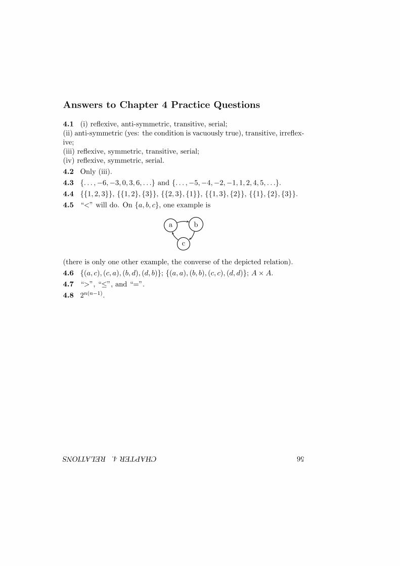
56CHAPTER4.RELATIONSAnswers to Chapter 4 Practice Questions
4.1 (i) reflexive, anti-symmetric, transitive, serial;(ii) anti-symmetric (yes: the condition is vacuously true), transitive, irreflex-ive;(iii) reflexive, symmetric, transitive, serial;(iv) reflexive, symmetric, serial.
4.2 Only (iii).
4.3 . . . ,−6,−3, 0, 3, 6, . . . and . . . ,−5,−4,−2,−1, 1, 2, 4, 5, . . ..4.4 1, 2, 3, 1, 2, 3, 2, 3, 1, 1, 3, 2, 1, 2, 3.4.5 “<” will do. On a, b, c, one example is
a b
c
(there is only one other example, the converse of the depicted relation).
4.6 (a, c), (c, a), (b, d), (d, b); (a, a), (b, b), (c, c), (d, d); A × A.
4.7 “>”, “≤”, and “=”.
4.8 2n(n−1).
Chapter 5
Sequences
Reading: Ross & Wright: 4.2, 4.4, 4.5, 4.6;Chetwynd & Diggle: not covered;Grimaldi: 4.1, 4.2;Grossman: 7.1–7.4.
Sequences, particularly sequences of numbers, occur in many computer sci-ence disciplines. Often, the sequence is specified by a recursive formula, andlater “solved” to find a closed form for the n-th term of the sequence. Inthis chapter we will explore some examples of sequences, and the importantproof technique called induction. Induction is often used to prove that aclosed form is the correct solution, but finding the closed form in the firstplace can be harder.
5.1 Definition
Sequences are usually infinite, and we write them as (x1, x2, . . .), but theyare best formalized as functions:
Definition A sequence is a function whose domain is N (or N+). Theargument of the function is usually written as a subscript, e.g. fn insteadof f(n). The entire sequence is denoted (fn).
57
58 CHAPTER 5. SEQUENCES
Sequences often have letters like (xn) or (an); when the sequence refers tothe time complexity of a program (the number of steps it takes to run)then it is usually (tn) or, abandoning the subscripted argument, T (n).
The obvious way to define a sequence is to give the function explicitly.For example, xn = 2n defines the sequence (2, 4, 6, 8, . . .) or (0, 2, 4, 6, . . .)(whether a sequence starts at 0 or 1, or even some other number, is a matterof convenience). Or ai = i2 gives the sequence (0, 1, 4, 9, 16, . . .). But se-quences are often defined recursively, by writing xn as a formula of some ofthe previous xi and then giving enough of the first few values of the sequencefor the rest to be determined.
Recursively-defined sequences include x0 = 0, xn+1 = xn + 2 (this definesthe same sequence as xn = 2n) and f0 = 1, fn+1 = (n + 1)fn (this is thesequence of factorials) but xn is allowed to depend on more than just theimmediately preceding sequence term. An important example is
Example 5.1 The Fibonacci sequence or (Fibonacci numbers) is thesequence given by
F0 = 0, F1 = 1, Fn+2 = Fn+1 + Fn.
The first few terms of the Fibonacci sequence are 0, 1, 1, 2, 3, 5, 8, 13, 21, 34, . . .
Example 5.2 The sequence xn defined by x0 = 0, and xn = x⌊n2⌋ + 1 for
n > 0, begins (0, 1, 2, 2, 3, 3, 3, 3, 4, . . .).
It is important to include cases to get the recursion started (they are calledboundary conditions): the sequences generated by yn+1 = 2yn, y0 = 0and y′n+1 = 2y′n, y′0 = 1 are completely different, and the Fibonacci recur-rence Fn+2 = Fn+1 + Fn does not define a sequence unless we specify thefirst two terms.
A sequence defined recursively is also known as a recurrence relation. Ifwe want to find a nonrecursive formula for the n-th term of a recursively-defined sequence, we speak of solving the recurrence relation.
In fact, it is possible to solve the preceding recurrence relations. The n-thFibonacci number Fn has the closed form
Fn = 1√5
(
1+√
52
)n − 1√5
(
1−√
52
)n
5.2. PROOF BY INDUCTION 59
and the sequence xn, above, has
xn = ⌊log2 n⌋ + 1
for n ≥ 1. You can probably see where the latter comes from, but the formermight seem rather mysterious (indeed it is not even obvious that the formulagives a whole number!). Methods to solve recurrences of the Fibonacci typeare briefly covered in Section 5.5.
Note that the same sequence might be specified by any number of differentrecurrences. For example, you can check that xn = n! is generated by eitherx0 = 1, xn+1 = (n + 1)xn or by x0 = 1, x1 = 1, xn+2 = (n + 1)(xn+1 + xn).
5.2 Proof by Induction
In many areas of mathematics and computer science we are asked to provethat some statement, which depends on a natural number n, is true for all n.Sometimes we can do so directly, but sometimes the proof depends so muchon the value of n that we seem forced to perform infinitely many differentproofs, one for each n. In such a situation, the method of induction can behelpful.
Principle of Induction: Let S(n) be a statement involving the naturalnumber n. If we prove S(0), and we prove that S(k + 1) is true wheneverS(k) is true, then this is sufficient to prove that S(n) for all n ∈ N.
When performing an induction we call the part which proves S(0) the basecase and the part which, assuming S(k), proves S(k + 1) the inductivestep. In the latter, the assumption that S(k) is true is known as the induc-tive hypothesis (often abbreviated as IH). It should be easy to understandwhy a proof by induction is correct: it shows that S(0) is true, so S(1) istrue, so S(2) is true, and eventually each S(n) is proved true. The principleholds because 0 ∈ N, and k ∈ N implies k + 1 ∈ N is really the definition ofthe set of natural numbers.
As an example of a proof by induction, we will prove a fact about a sequence.
Example 5.3 Recall the Fibonacci numbers: F0 = 0, F1 = 1, Fn+2 =Fn+1 + Fn. We can prove that 2 |F3n for each n ∈ N by induction on n.
60 CHAPTER 5. SEQUENCES
First, the base case n = 0. We need to prove that 2 |F0: F0 = 0, and 0 is amultiple of 2, so we are done.
Second, the inductive step. Suppose that we have already proved that 2 |F3k:we need to prove that 2 |F3k+3. Using the recurrence relation which definedFn, we calculate
F3k+3 = F3k+2 + F3k+1
= 2F3k+1 + F3k
= 3F3k + 2F3k−1
But remember we have assumed that F3k is even, and 2F3k−1 is certainlyeven, so we have proved that 2 |F3k+3. That completes the proof by induc-tion.
If we are to prove that something holds for n ≥ 1 (or more generally n ≥ m)we merely modify the base case to be n = 1 (or n = m). In fact, other proofsby induction are possible: if we prove S(0) and S(1), and that S(k) impliesS(k + 2), then we have covered all of N. More complex alternatives arepossible, but rare in practice when trying to prove a result for all n ∈ N. Itis also possible to use induction to prove that something is true for membersof other sets, and then the structure of the set determines the structure of theinductive proof. We will not see examples of these “structural” inductionsin this course, but they are very common in Functional Programming.
One slightly modified type of induction we will need is sometimes calledstrong induction.
Principle of Strong Induction: Let S(n) be a statement involving thenatural number n. If we prove S(0), and we prove that S(k + 1) is trueassuming that S(j) is true for all j ≤ k, then this is sufficient to prove thatS(n) for all n ∈ N.
An example of a strong induction is:
Claim 5.4 Every n ∈ N+ can be written as the sum of distinct Fibonaccinumbers.
Proof The base case is n = 1, which is just a single Fibonacci number(F1); nothing to prove.
For the inductive step, we may assume that each of 1, 2, 3, . . . , k can all bewritten as the sum of distinct Fibonacci numbers and we must prove that

5.3. SIGMA NOTATION AND SUMS OF SEQUENCES 61
the same is true of k + 1. If k + 1 is already a Fibonacci number, we arefinished. If not, k+1 lies between two consecutive Fibonacci numbers Fj andFj+1 (the Fibonacci sequence increases indefinitely), i.e. Fj < k +1 < Fj+1.
Write k + 1 = Fj + (k + 1 − Fj). Since k + 1 − Fj ≤ k, the inductivehypothesis tells us that k + 1 − Fj can be written as the sum of distinctFibonacci numbers. Now remember that k + 1 < Fj+1 = Fj + Fj−1 (usingthe Fibonacci recurrence) so k + 1 − Fj < Fj−1. This means that none ofthe distinct Fibonacci numbers which sum to k + 1 − Fj could possibly beFj , or the sum would be too big. Thus we can write k + 1 as a sum ofdistinct Fibonacci numbers: Fj plus all those which sum to k +1−Fj . Thiscompletes the proof by induction.
A proof technique closely related to induction is called the minimal coun-terexample. It is a form of proof by contradiction. If we want to provethat something is true for all n, we suppose (for a contradiction) that itis not true. Then we examine the smallest n for which it is false, tryingto deduce that, in fact, it must be false for a smaller n as well. That is acontradiction. This is best illustrated by a simple example
Claim 5.5 The recurrence x1 = 1, x2 = 3, xn+2 = 4xn+1 + 3xn generatesa sequence of odd numbers.
Proof This can easily be proved by induction, but even quicker is to usethe minimal counterexample technique. Suppose that xm is the first evennumber in the sequence. m cannot be 1 or 2, so xm = 4xm−1 +3xm−2. Thisimplies that xm−2 is even, a contradiction with the assumption that xm wasthe first even number in the sequence. Therefore there cannot be any evennumbers in the sequence.
5.3 Sigma Notation and Sums of Sequences
First, some standard mathematical notation.
Definition If (an) is a sequence then we can write∑n
i=m ai as a shorthandfor the sum of the segment am + am+1 + · · ·+ an. Analogously, the notation∏n
i=m ai is the product am · am+1 · · · an.
62 CHAPTER 5. SEQUENCES
This notation can be extended to∑∞
i=1 ai, which performs the infinite sum-mation, but analysis of infinite sums or products (whose values are notnecessarily defined) is beyond the scope of this course.
For example, we have∑4
i=1 i2 = 12 + 22 + 32 + 42 = 30, and∏4
i=2(i + 1) =3 · 4 · 5 = 60. Given a sequence ai, we can generate a new sequence calledthe partial sums of ai defined by sn =
∑ni=1 ai and, using induction, we
can sometimes give a simple formula for the partial sums of a sequence. Forexample, the sum of the first n square integers:
Claim 5.6 For n ∈ N+,∑n
i=1 i2 = n(n+1)(2n+1)6 .
Proof (The result is also true for n = 0 if we adopt the standard conventionthat a sum of no terms equals zero.)
This is a classic example of proof by induction. For the base case (n = 1)the left side is 1 and the right side is 6/6.
For the inductive step, suppose the result is true for n = k and look atn = k + 1:
∑k+1i=1 i2 =
∑ki=1 i2 + (k + 1)2 extracting the final term
= k(k+1)(2k+1)6 + (k + 1)2 by the inductive hypothesis
= (k+1)(k(2k+1)+6(k+1))6 rearranging
= (k+1)(k+2)(2k+3)6 factorising
and this is exactly the statement for n = k + 1. That completes the proofby induction.
This demonstrates that proofs by induction often have the flavour of ver-ifying a formula, rather than finding it: we could not have attempted theproof without knowing, or guessing, the value of the sum.
5.4 Sequences Associated with Counting
Recurrence relations arise in counting problems, and sometimes it is possibleto use some ingenious reasoning to find a recursive formula for counting someset when direct methods fail.
We have already met the derangements, in Chapter 3. Instead of the com-binatorial formula derived there, the number of derangements of n objectsdn can be described by a recurrence relation.
5.4. SEQUENCES ASSOCIATED WITH COUNTING 63
Claim 5.7 The sequence dn satisfies
d1 = 0, d2 = 1, dn = (n − 1)(dn−1 + dn−2) for n ≥ 2.
Proof That d1 = 0 and d2 = 1 is immediate from the definition of thederangements. We must then argue that dn = (n − 1)(dn−1 + dn−2).
Consider a derangement on objects 1, 2, . . . , n, and suppose that object nis found in place i: there are n − 1 possibilities for i (object n cannot bein place n). Now if we swap object n and object i there are two exclusivecases:
• After swapping n and i, the first n − 1 objects still form a derangement.
• After swapping n and i, the first n−1 objects do not form a derangement.
There are dn−1 ways in which the former can happen and in the latter,because we supposed that we began with a derangement on all n objects,the only way we can fail to have a derangement is if we now have object iin place i leaving dn−2 derangements of the other elements. In total, then,(n − 1)(dn−1 + dn−2) derangements of all n objects.
It is interesting to note that the recurrence dn = (n − 1)(dn−1 + dn−2) isalso satisfied by the factorial function (which counts the total number ofpermutations, whether derangements or not) if the boundary condition isaltered.
Another sequence associated with counting is
Definition The number of partitions of a set with cardinality n is writtenBn. The sequence B0, B1, . . . is known as the Bell numbers (after the sci-fiauthor and mathematician Eric Temple Bell) and begins 1, 1, 2, 5, 13. . . ..
It is difficult to find a closed form for Bn, but we can give a recurrencerelation which enables the sequence to be computed step-by-step.
Claim 5.8 The Bell numbers are generated by: B0 = 1,
Bn+1 =n
∑
i=0
(
n
i
)
Bi.
Proof There is only one set with zero cardinality (∅) and only one partition
64 CHAPTER 5. SEQUENCES
of it.
Now consider a set of cardinality n + 1, say A = a1, . . . , an+1. Considerwhat happens to an+1 in a partition of A:
• an+1 could be a singleton set in the partition. In that case there are Bn
ways to partition the other n elements, to which an+1 is added to makea partition of A.
• an+1 could be in a set with exactly one other element ai, in the partition.There are n =
(
n1
)
choices for this other element, and for any such choicethere are Bn−1 ways to partition the other n− 1 elements of A, to whichai, an+1 is added to make a partition of A.
• an+1 could be in a set with exactly two other elements ai, aj , in thepartition. There are
(
n2
)
choices for these other elements, and for anysuch choice there are Bn−2 ways to partition the other n− 2 elements ofA, to which ai, aj , an+1 is added to make a partition of A.
• ...
• an+1 could be in a set with exactly n− 1 other elements in the partition.There are
(
nn−1
)
choices for these elements, and for any such choice thereare B1 ways to partition the other element of A.
• an+1 could be in a set with all n other elements in the partition. Thereis 1 =
(
nn
)
choice.
These cases are disjoint, so we can add up all the choices giving∑n
i=0
(
ni
)
Bi
different partitions of A. (Here we used(
nk
)
=(
nn−k
)
.)
The mathematician Dobinski proved, in the 1870s, that the Bell numberscan be given by the infinite sum
Bn =1
e
∞∑
k=0
kn
k!.
Even though an infinite sum seems a rather pointless “solution”, this for-mula draws an interesting connection between Bell numbers and the Poissondistribution found in probability.
You might be able to convince yourself that Dobinski’s formula is cor-rect by substituting this formula into the right hand side of the recurrence

5.5. SOLVING LINEAR RECURRENCE RELATIONS 65
∑ni=0
(
ni
)
Bi and rearranging. If you use the binomial theorem
(a + b)n =n
∑
i=0
(
n
i
)
aibn−i
you can reduce to 1e
∑∞k=0
kn+1
k! , suggesting that the Dobinski formula doessatisfy the required recurrence. But infinite sums cannot always be manipu-lated in the same way as finite sums, and you need some more mathematics,not covered in this course, to make the calculation into a proper proof.
5.5 Interesting Diversion:
Solving Linear Recurrence Relations
One class of recurrence relations is both common and reasonably easy tosolve. These are the constant-coefficient linear recurrence relations. Therenow follows a quick primer on how to solve them; the reasoning behind themethod will not be included. You may find these methods useful in theprobability course.
First, the homogeneous constant-coefficient linear recurrences. They havethe form
λmxn + λm−1xn−1 + · · · + λ0xn−m = 0, (5.1)
where all the λi are real numbers, plus some boundary conditions (usuallym are required.) Examples include xn+1 = 3xn (which can be rewritten inthe form xn −3xn−1 = 0), xn −xn−1 −xn−2 = 0 (the Fibonacci recurrence),and xn + 3xn−1 + 3xn−2 + xn−3 = 0.
To solve these recurrences, try a solution of the form xn = rn, where r is aconstant. Substituting into (5.1) and dividing through by rm−n we have
λmrm + λm−1rm−1 + · · · + λ0 = 0. (5.2)
This is called the characteristic polynomial. Note that any value of rsatisfying (5.2) will give a solution of (5.1).
Find all the roots r1, r2, . . . , rm of the characteristic polynomial (includingcomplex roots, if there are any). As long as all these roots are distinct,all solutions of (5.1) will be of the form xn = A1r
n1 + A2r
n2 + · · · + Amrn
m,
66 CHAPTER 5. SEQUENCES
where the A’s are constants. The boundary conditions of the recurrence willdetermine the A’s. If some of the roots are repeated, add extra multiplesof n to the repeat factors until they are all distinct. For example, if thecharacteristic polynomial factorizes as (r − 2)2(r − 3)3 then the solutions to(5.1) will be of the form xn = A12
n + A2n2n + A33n + A4n3n + A5n
23n.
Example 5.9 Consider the linear homogeneous recurrence
xn − 4xn−1 + 5xn−2 − 2xn−3 = 0, x0 = 0, x1 = 1, x2 = 2.
The characteristic polynomial is r3 − 4r2 + 5r − 2 = 0, which factorizes as(r − 1)2(r − 2). Therefore the general solution of the recurrence, withoutany boundary conditions, is
xn = A + Bn + C2n
(because 1 is a repeated root of the characteristic polynomial we need theterms A1n and Bn1n). Now substitute into the boundary conditions: wehave 0 = A + C, 1 = A + B + 2C, 2 = A + 2B + 4C. Solving these threesimultaneous equations gives A = 0, B = 1, C = 0, so in fact the solutionto the original recurrence relation is just xn = n.
We might want to solve an inhomogeneous constant-coefficient linear re-currence. This is of the form
λmxn + λm−1xn−1 + · · · + λ0xn−m = f(n), (5.3)
plus some boundary conditions (again usually m of them). Note that if yn
is a solution of the homogeneous recurrence (without the term f(n)) and zn
is a solution of the inhomogeneous recurrence, then xn +zn is also a solutionof the inhomogeneous recurrence.
We begin by “guessing” a solution to the inhomogeneous recurrence, withoutregard to the boundary conditions. Experience shows that when f(n) is apolynomial of degree n, we should guess a polynomial of degree n, and iff(n) = an we should guess a multiple of an, and you can find other rulesof thumb in textbooks. Then solve the homogeneous recurrence, withoutregard to boundary conditions. Finally, add together the two solutions, anduse the boundary conditions to determine any missing constants.
5.5. SOLVING LINEAR RECURRENCE RELATIONS 67
Example 5.10 Consider the linear inhomogeneous recurrence
xn − 2xn−1 = 3n + 5n, x0 = 0.
Because of the form of the inhomogeneity, we “guess” that xn = A3n +Bn + C will find a solution. Substituting into the recurrence, we obtain theequation
A3n + Bn + C − 2A3n−1 − 2B(n − 1) − 2C = 3n + 5n
and equating coefficients gives: (3n) A = 3, (n) B = −5, (1) C = −10, so wehave found the solution zn = 3n+1 − 5n − 10. But this does not yet satisfythe boundary condition.
We solve the homogeneous recurrence yn − 2yn−1 = 0, which is straight-forwardly given by yn = D2n for any D. Then we try xn = yn + zn =D2n + 3n+1 − 5n − 10 against the boundary condition, finding that D = 7.We have solved the original recurrence by
xn = 7 · 2n + 3n+1 − 5n − 10.
Finally, we mention in passing that there is another technique for solvingrecurrences called generating functions. They are a powerful tool forcertain types of recurrence, including nonlinear recurrences where the abovetechniques do not apply, but they do not appear in this course.

68 CHAPTER 5. SEQUENCES
Practice Questions
5.1 Find recurrence relations which generate the sequences
(i) (1, 4, 16, 64, 256, . . .);
(ii) (1, 4, 9, 16, 25, 36, 49, . . .);
(iii) xn = ⌊log3 n⌋ (for n ≥ 1).
5.2 Find, using the techniques of Section 5.5, or simply by guessing thesolution and proving by induction, the solution to the recurrence u0 = 0,u1 = 1, un+2 = 2un+1 − un + 1.
5.3 Show, by induction on n, that xn = 2n − 1 solves the recurrencex1 = 1, xn+1 = 2xn + 1.
5.4 Prove, by induction on n, that 11·4 + 1
4·7 + · · · + 1(3n−2)(3n+1) = n
3n+1for n ≥ 1.
5.5 Using the recurrence relation for the Bell numbers, compute B5.
5.6 If the recurrence relation for the number of derangements, dn = (n −1)(dn−1 + dn−2), d1 = 0, d2 = 1, is to be extended to d0, what must be thevalue of d0 for the recurrence still to hold? Does this make sense?
5.7 Find the solutions of
(i) x0 = 1, xn+1 = 3xn;
(ii) x1 = 1, x2 = 1, xn+2 = 3xn+1 − 2xn;
(iii) x0 = 0, x1 = 0, x2 = 0, xn+3 = 16xn+2 + 15xn+1 + 14xn.
(They do not require proof.)
5.8 Using the techniques in Section 5.5, find the solution of x1 = 1, x2 = 3,xn+2 = 3xn+1 − 2xn

PRACTICE QUESTIONS 69

70CHAPTER5.SEQUENCESAnswers to Chapter 5 Practice Questions
5.1 There are many answers, but the simplest are (i) x0 = 1, xn+1 = 4xn;(ii) x0 = 1, xn+1 = xn + 2n + 1; (iii) x1 = 0, x2 = 0, xn = x⌊n/3⌋ + 1 forn ≥ 3.
5.2 un = n(n + 1)/2.
5.3 The base case is n = 1: 21 − 1 = 1 = x1. Suppose the result forn = k. Then the right-hand side of the recurrence 2xk + 1, substituting theIH, equals 2(2k − 1) + 1, which equals 2k+1 − 1 as required. That completesthe induction.
5.4 The base case is n = 1: the left hand side is 14 and the right
hand side is 13·1+1 . For the inductive step, suppose that 1
1·4 + 14·7 +
· · · + 1(3k−2)(3k+1) = k
3k+1 . Now compute 11·4 + 1
4·7 + · · · + 1(3k−2)(3k+1) +
1(3k+1)(3k+4) = k
3k+1 + 1(3k+1)(3k+4) . Simplifying, this equals k(3k+4)+1
(3k+1)(3k+4) =
3k2+4k+1(3k+1)(3k+4) = (3k+1)(k+1)
(3k+1)(3k+4) = k+13(k+1)+1 . This is the required result for k + 1.
That completes the proof by induction.
5.5 B5 =(
40
)
1 +(
41
)
1 +(
42
)
2 +(
43
)
5 +(
44
)
15 = 52.
5.6 d0 = 1. This makes sense because the only partition of the empty setdoes not leave element i in place i (there is no element i to leave in placei!).
5.7 (i) xn = 3n; (ii) xn = 1; (iii) xn = 0.
5.8 xn = 2n+1 − 1.
Chapter 6
Modular Arithmetic
Reading: Ross & Wright: 3.5, 4.7, 5.5;Chetwynd & Diggle: only 3.9 (mostly not covered);Grimaldi: 4.4, 5.5, 14.3;Grossman: 12.1–12.4.
When arithmetic is performed on the remainder, after division by a fixednumber n, this is known as modular arithmetic, and n is called the mod-ulus. This topic is usually considered part of pure mathematics (the branchknown as number theory) and this chapter is the most mathematical of thecourse. But modular arithmetic has applications in computer science algo-rithms, particularly for computing with very large numbers, testing whethera number is prime (vital for encryption), and coding for reliable informationtransmission over a noisy network.
6.1 Definitions
We begin with a relation on Z. Fix n ∈ N+, then write x ≡ y (mod n) ifn | (x−y). This is equivalent to saying that x and y have the same remainderwhen divided by n. It is easy to see that this is an equivalence relation: xcertainly has the same remainder as x (reflexivity); if x and y have the sameremainder, so do y and x (symmetry); if x and y have the same remainder,and so do y and z, then x and z have the same remainder (transitivity).
71
72 CHAPTER 6. MODULAR ARITHMETIC
The equivalence classes are easy to compute: any x is related to x−2n, x−n,x, x + n, x + 2n, etc, so the n equivalence classes are [0], [1], . . . , [n − 1].
Now for some arithmetic.
Claim 6.1 If x1 ≡ x2 (mod n) and y1 ≡ y2 (mod n), then
(i) x1 + y1 ≡ x2 + y2 (mod n), and
(ii) x1y1 ≡ x2y2 (mod n).
Proof We have n | (x1 − x2) so x1 − x2 = kn for k ∈ Z, and n | (y1 − y2)so y1 − y2 = ln for l ∈ Z.
(i) Adding, we deduce x1+y1−x2−y2 = (k+l)n, so n |(
(x1+y1)−(x2+y2))
.
(ii) Multiplying by y1 and then again by x2, we have x1y1 − x2y2 = (x1 −x2)y1 + x2(y1 − x2) = (ky1 + x2l)n so n | (x1y1 − x2y2).
This allows us to define the operations of addition and multiplication mod-ulo n, on the equivalence classes: [x] + [y] = [x + y] and [x] · [y] = [xy]. Wehave proved that the answers do not depend on which members of [x] and[y] are chosen to represent the class. Equivalently, we have defined additionand multiplication binary operators on the set Zn.
This is modular arithmetic (mod n), in which multiples of n are discardedand only the remainders kept. An example of a calculation in modulararithmetic is
13 · 15 + 17 ≡ 4 · 6 + 8 ≡ 32 ≡ 5 (mod 9).
In modular arithmetic calculations we can replace any number by anotherwith the same remainder after division by the modulus. Usually we removeall multiples of the modulus (this is called reduction (mod n)) but some-times it is convenient reduce numbers to negative remainders. For example,an equivalent calculation is
13 · 15 + 17 ≡ (4 · −3) − 1 ≡ −13 ≡ 5 (mod 9).
Negative numbers (and subtraction) do exist in modular arithmetic; becausen − x ≡ −x mod n, every number does have a negative (mathematicianscall −x an additive inverse). The situation is not so simple for division,as we shall see later.
6.2. EXPONENTIATION 73
6.2 Exponentiation
Having seen that the result of addition and multiplication (mod n) requireonly the remainders of the arguments, it is natural to assume that the sameapplies to exponentiation. It does not, quite.
Claim 6.2 If x1 ≡ x2 (mod n) and y ∈ Z then
(i) xy1 ≡ xy
2 (mod n), but
(ii) yx1 ≡ yx2 (mod n) need not hold.
Proof (i) By x1 ≡ x2 (mod n) and the rule for modular multiplication wehave x2
1 ≡ x22 (mod n), so x3
1 ≡ x32 (mod n), and so on. (It is also true for
x01 = 1 = x0
2). This proof can be formalised by induction.
(ii) The simplest counterexample is 00 = 1 and 02 = 0 with n = 2. (It iscorrect that 00 = 1, but there are many other counterexamples if this onelooks like a technicality.)
Therefore we can say that 1312 ≡ 312 (mod 10), but it is not true that1312 ≡ 132 (mod 10) (check for yourself). In fact, there are different lawsfor exponentiation, which are not very hard to prove but beyond the scopeof this course. When p is a prime number, we can guarantee yx1 ≡ yx2
(mod p) as long as x1 ≡ x2 (mod p − 1); it seems a bit strange that oneequation (mod p) is connected to another (mod p− 1), until you get used toit! This law, and its extensions, are the heart of the well-known public keyencryption scheme RSA.
If we have to compute a large exponentiation, for example x600 (mod 11),we can reduce x mod n, but would like to avoid computing the 600th powerto find the remainder. This is possible using the method of repeatedsquaring, which amounts to the recurrence
xy =
1 if y = 0
x · (x2)y−12 if y is odd
(x2)y
2 if y > 0 is even
which is true for integers x and y ≥ 0. So to compute 2600 (mod 11), wecan apply the recurrence repeatedly and reduce the base of the exponent at
74 CHAPTER 6. MODULAR ARITHMETIC
each stage:
2600 ≡ (22)300 ≡ 4300 (mod 11)≡ (42)150 ≡ 5150 (mod 11)≡ (52)75 ≡ 375 (mod 11)≡ 3 · (32)37 ≡ 3 · 937 (mod 11)≡ 3 · 9 · (92)18 ≡ 5 · 418 (mod 11)≡ 5 · (42)9 ≡ 510 (mod 11)≡ (52)5 ≡ 35 (mod 11)≡ 3 · (32)2 ≡ 3 · 92 (mod 11)≡ 3 · 4 ≡ 1 (mod 11).
We end with a little observation about squares (mod 4). Since we knowthat the remainder of x (mod 4) determines the remainder of x2 (mod 4),consider all the possibilities:
02 ≡ 0 (mod 4), 12 ≡ 1 (mod 4), 22 ≡ 0 (mod 4), 32 ≡ 1 (mod 4).
So always x2 ≡ 0 or 1 (mod 4): a square number can never have remainder2 or 3 when divided by 4.
6.3 mod and div
We briefly consider two binary operators on (positive) integers, which arerelated to modular arithmetic.
Definition mod : N×N+ → N and div : N×N+ → N are written infixand defined by:
m mod n = the remainder when m is divided by nm div n = ⌊m/n⌋
More usefully, we have the equation m = n·(m div n)+m mod n, expressingm uniquely as an integer multiple of n plus a remainder term.
We have introduced these functions because most programming languagesprovide them as primitives (mod is often the symbol “%”). Many languagesattempt to extend the domains to Z2, but unfortunately it is not clear what
6.4. EUCLID’S ALGORITHM AND MULTIPLICATIVE INVERSES 75
the answers should be when the arguments are negative (particularly themodulus): the meaning of 3 mod (−2) is not obvious. Different languagesmay implement different functionality, so it is sensible to exercise cautionwhen using div and mod operators, whatever they are called in your pro-gramming language of choice, on signed numbers.
6.4 Euclid’s Algorithm and Multiplicative Inverses
Recall the relation m |n (m divides n). Whether a number divides anotheris at the heart of modular arithmetic, and it is often important to find thelargest integer which divides a set of numbers.
Definition For m, n ∈ N+ the greatest common divisor (gcd) of mand n, written gcd(m, n), is the greatest integer g which satisfies both g |mand g |n.
If gcd(m, n) = 1 then m and n are said to be coprime (in some books,relatively prime).
The definition extends to any set of positive integers: gcd(m1, m2, . . . , mn)is the greatest integer g for which g |mi for all i, and a set is called coprimeif its gcd is 1.
(An equivalent definition, sometimes more convenient, is that gcd(m, n) = gif i) g |m, ii) g |n, and iii) l |m and l |n together imply l | g.)
For example, gcd(12, 10) = 2, gcd(9, 3) = 3, gcd(5, 14) = 1 (5 and 14 arecoprime).
A few notes about divisors. Recall that an integer p > 1 is called a primenumber if its only divisors are 1 and p (i.e. m | p implies m = 1 or m = p).The number 1 is not considered to be a prime number. Now if n < p isanother positive integer, we must have gcd(n, p) = 1: n and p cannot haveany common divisors greater than 1 if p does not have any other divisors.
Let us consider how to compute the greatest common divisor of a pair ofintegers. It is rather hard work to find all the divisors of m and n, and thenlook for the greatest, if m and n are large numbers. And, when we wantto compute gcds in practice (e.g. for cryptography purposes), they often
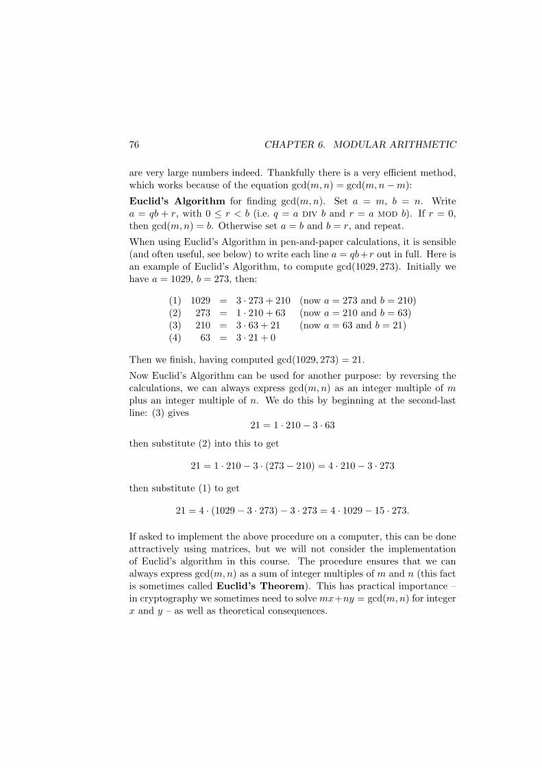
76 CHAPTER 6. MODULAR ARITHMETIC
are very large numbers indeed. Thankfully there is a very efficient method,which works because of the equation gcd(m, n) = gcd(m, n − m):
Euclid’s Algorithm for finding gcd(m, n). Set a = m, b = n. Writea = qb + r, with 0 ≤ r < b (i.e. q = a div b and r = a mod b). If r = 0,then gcd(m, n) = b. Otherwise set a = b and b = r, and repeat.
When using Euclid’s Algorithm in pen-and-paper calculations, it is sensible(and often useful, see below) to write each line a = qb+r out in full. Here isan example of Euclid’s Algorithm, to compute gcd(1029, 273). Initially wehave a = 1029, b = 273, then:
(1) 1029 = 3 · 273 + 210 (now a = 273 and b = 210)(2) 273 = 1 · 210 + 63 (now a = 210 and b = 63)(3) 210 = 3 · 63 + 21 (now a = 63 and b = 21)(4) 63 = 3 · 21 + 0
Then we finish, having computed gcd(1029, 273) = 21.
Now Euclid’s Algorithm can be used for another purpose: by reversing thecalculations, we can always express gcd(m, n) as an integer multiple of mplus an integer multiple of n. We do this by beginning at the second-lastline: (3) gives
21 = 1 · 210 − 3 · 63
then substitute (2) into this to get
21 = 1 · 210 − 3 · (273 − 210) = 4 · 210 − 3 · 273
then substitute (1) to get
21 = 4 · (1029 − 3 · 273) − 3 · 273 = 4 · 1029 − 15 · 273.
If asked to implement the above procedure on a computer, this can be doneattractively using matrices, but we will not consider the implementationof Euclid’s algorithm in this course. The procedure ensures that we canalways express gcd(m, n) as a sum of integer multiples of m and n (this factis sometimes called Euclid’s Theorem). This has practical importance –in cryptography we sometimes need to solve mx+ny = gcd(m, n) for integerx and y – as well as theoretical consequences.
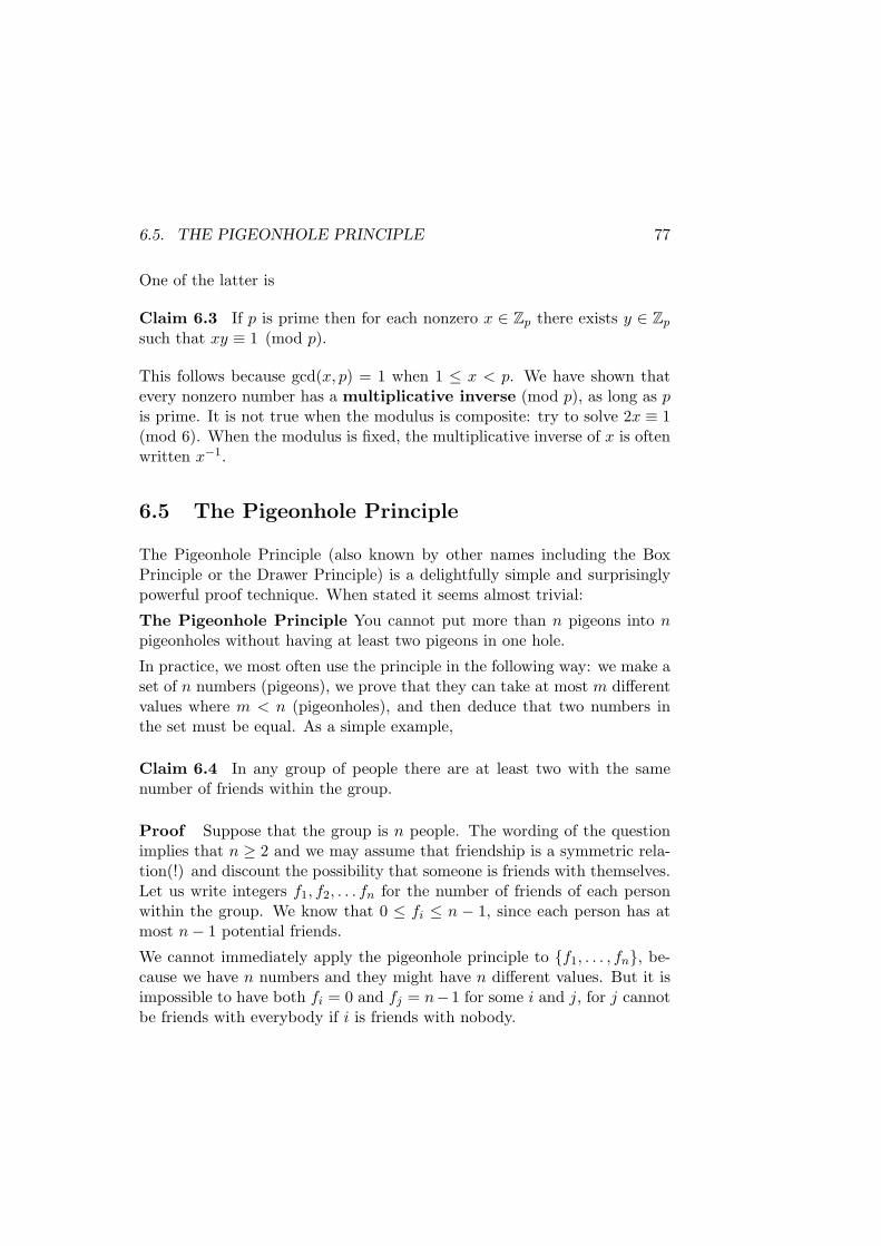
6.5. THE PIGEONHOLE PRINCIPLE 77
One of the latter is
Claim 6.3 If p is prime then for each nonzero x ∈ Zp there exists y ∈ Zp
such that xy ≡ 1 (mod p).
This follows because gcd(x, p) = 1 when 1 ≤ x < p. We have shown thatevery nonzero number has a multiplicative inverse (mod p), as long as pis prime. It is not true when the modulus is composite: try to solve 2x ≡ 1(mod 6). When the modulus is fixed, the multiplicative inverse of x is oftenwritten x−1.
6.5 The Pigeonhole Principle
The Pigeonhole Principle (also known by other names including the BoxPrinciple or the Drawer Principle) is a delightfully simple and surprisinglypowerful proof technique. When stated it seems almost trivial:
The Pigeonhole Principle You cannot put more than n pigeons into npigeonholes without having at least two pigeons in one hole.
In practice, we most often use the principle in the following way: we make aset of n numbers (pigeons), we prove that they can take at most m differentvalues where m < n (pigeonholes), and then deduce that two numbers inthe set must be equal. As a simple example,
Claim 6.4 In any group of people there are at least two with the samenumber of friends within the group.
Proof Suppose that the group is n people. The wording of the questionimplies that n ≥ 2 and we may assume that friendship is a symmetric rela-tion(!) and discount the possibility that someone is friends with themselves.Let us write integers f1, f2, . . . fn for the number of friends of each personwithin the group. We know that 0 ≤ fi ≤ n − 1, since each person has atmost n − 1 potential friends.
We cannot immediately apply the pigeonhole principle to f1, . . . , fn, be-cause we have n numbers and they might have n different values. But it isimpossible to have both fi = 0 and fj = n−1 for some i and j, for j cannotbe friends with everybody if i is friends with nobody.
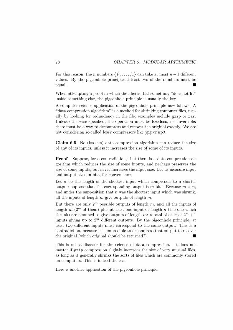
78 CHAPTER 6. MODULAR ARITHMETIC
For this reason, the n numbers f1, . . . , fn can take at most n− 1 differentvalues. By the pigeonhole principle at least two of the numbers must beequal.
When attempting a proof in which the idea is that something “does not fit”inside something else, the pigeonhole principle is usually the key.
A computer science application of the pigeonhole principle now follows. A“data compression algorithm” is a method for shrinking computer files, usu-ally by looking for redundancy in the file; examples include gzip or rar.Unless otherwise specified, the operation must be lossless, i.e. invertible:there must be a way to decompress and recover the original exactly. We arenot considering so-called lossy compressors like jpg or mp3.
Claim 6.5 No (lossless) data compression algorithm can reduce the sizeof any of its inputs, unless it increases the size of some of its inputs.
Proof Suppose, for a contradiction, that there is a data compression al-gorithm which reduces the size of some inputs, and perhaps preserves thesize of some inputs, but never increases the input size. Let us measure inputand output sizes in bits, for convenience.
Let n be the length of the shortest input which compresses to a shorteroutput; suppose that the corresponding output is m bits. Because m < n,and under the supposition that n was the shortest input which was shrunk,all the inputs of length m give outputs of length m.
But there are only 2m possible outputs of length m, and all the inputs oflength m (2m of them) plus at least one input of length n (the one whichshrunk) are assumed to give outputs of length m: a total of at least 2m + 1inputs giving up to 2m different outputs. By the pigeonhole principle, atleast two different inputs must correspond to the same output. This is acontradiction, because it is impossible to decompress that output to recoverthe original (which original should be returned?).
This is not a disaster for the science of data compression. It does notmatter if gzip compression slightly increases the size of very unusual files,as long as it generally shrinks the sorts of files which are commonly storedon computers. This is indeed the case.
Here is another application of the pigeonhole principle.
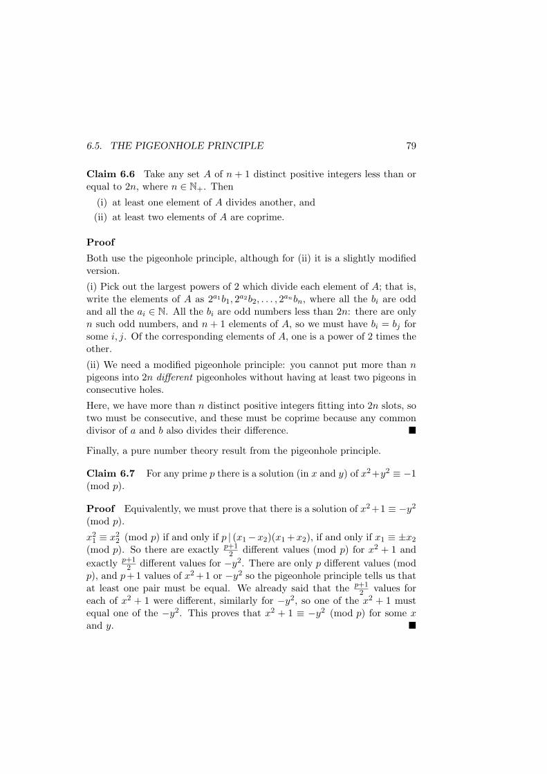
6.5. THE PIGEONHOLE PRINCIPLE 79
Claim 6.6 Take any set A of n + 1 distinct positive integers less than orequal to 2n, where n ∈ N+. Then
(i) at least one element of A divides another, and
(ii) at least two elements of A are coprime.
Proof
Both use the pigeonhole principle, although for (ii) it is a slightly modifiedversion.
(i) Pick out the largest powers of 2 which divide each element of A; that is,write the elements of A as 2a1b1, 2
a2b2, . . . , 2anbn, where all the bi are odd
and all the ai ∈ N. All the bi are odd numbers less than 2n: there are onlyn such odd numbers, and n + 1 elements of A, so we must have bi = bj forsome i, j. Of the corresponding elements of A, one is a power of 2 times theother.
(ii) We need a modified pigeonhole principle: you cannot put more than npigeons into 2n different pigeonholes without having at least two pigeons inconsecutive holes.
Here, we have more than n distinct positive integers fitting into 2n slots, sotwo must be consecutive, and these must be coprime because any commondivisor of a and b also divides their difference.
Finally, a pure number theory result from the pigeonhole principle.
Claim 6.7 For any prime p there is a solution (in x and y) of x2+y2 ≡ −1(mod p).
Proof Equivalently, we must prove that there is a solution of x2 +1 ≡ −y2
(mod p).
x21 ≡ x2
2 (mod p) if and only if p | (x1 −x2)(x1 +x2), if and only if x1 ≡ ±x2
(mod p). So there are exactly p+12 different values (mod p) for x2 + 1 and
exactly p+12 different values for −y2. There are only p different values (mod
p), and p+1 values of x2 +1 or −y2 so the pigeonhole principle tells us thatat least one pair must be equal. We already said that the p+1
2 values foreach of x2 + 1 were different, similarly for −y2, so one of the x2 + 1 mustequal one of the −y2. This proves that x2 + 1 ≡ −y2 (mod p) for some xand y.
80 CHAPTER 6. MODULAR ARITHMETIC
6.6 Interesting Diversion: Modular Square Roots
of -1
For a bonus, we prove a pure number theoretic result using the facts con-necting equivalence relations and partitions.
Claim 6.8 If p is prime, then x2 ≡ −1 (mod p) has a solution if and onlyif p = 2 or p ≡ 1 (mod 4).
Proof If p = 2 then x = 1 is a solution (in fact the only solution, up toequality (mod 2)).
For odd p, we construct an equivalence relation on 1, 2, . . . , p − 1:
y1 ∼ y2 if y1 ≡ ±y2 (mod p) or y1 ≡ ±y−12 (mod p).
It is easy to check that this does indeed define an equivalence relation. Eachequivalence class of ∼ can have up to four elements: y,−y, y−1,−y−1, butit is possible that these are not four distinct numbers:
(i) It is impossible to have y ≡ −y (mod p) when p is odd.
(ii) y ≡ y−1 (mod p) and −y ≡ −y−1 (mod p) (one of these happens ifand only if the other does). These are equivalent to y2 ≡ 1 (mod p),i.e. p | (y2 − 1) = (y − 1)(y + 1). This happens only when y ≡ ±1(mod p), so there is always one equivalence class with exactly twoelements: 1,−1.
(iii) y ≡ −y−1 (mod p) and −y ≡ y−1 (mod p) (again, each of these im-plies the other). They are equivalent to y2 ≡ −1 (mod p). Theremight be a solution to this equation or there might not, but there canonly be zero or two solutions to equations of this form (proof: y2 ≡ ais equivalent to (y − b)(y + b) ≡ 0: y ≡ ±b are the only solutions, ifany such b exists at all), so there may be one further equivalence classof size two y,−y, or there may be no further equivalence class ofsize two.
So there are always one (if y2 ≡ −1 has no solution) or two (if y2 ≡ −1has two solutions) equivalence classes of size 2, and all the other equivalenceclasses must be of size 4.
Now remember that the equivalence classes partition the set on which theequivalence relation is defined, here 1, 2, . . . , p−1. The cardinality is p−1,

6.6. MODULAR SQUARE ROOTS OF -1 81
and so the cardinality of the equivalence classes adds up to p−1. If p−1 ≡ 0(mod 4) then there must be two equivalence classes of size 2, so there is ay satisfying y2 ≡ −1 (mod p). On the other hand, if p − 1 ≡ 2 (mod 4)then there must be one equivalence class of size 2, so there is no solution ofy2 ≡ −1 (mod p).
82 CHAPTER 6. MODULAR ARITHMETIC
Practice Questions
6.1 Compute the remainder when (34 · 45 · 57 + 89)2 is divided by 8.
6.2 Compute the remainder when 1317 is divided by 11.
6.3 Use Euclid’s Algorithm to find the gcd of 805 and 105.
6.4 Use Euclid’s Algorithm to find integers x and y satisfying 21x+99y =3.
6.5 Show that gcd(Fn+1, Fn) = 1 (where Fn is the n-th Fibonacci num-ber). Use proof by induction on n.
6.6 Show that 14 cannot be written as the sum of two squares. Write itas the sum of three squares.
6.7 Consider an equilateral triangle which has sides of length 1 unit, andfive points placed in the triangle. Show that, no matter where the pointsare placed, at least two of them must be no more than 1
2 units apart.
6.8 Suppose we are given a finite set S ⊂ N. If log2 n < |S |, show thatthere exist two distinct subsets of S, S1 and S2, satisfying
∏
a∈S1
a =∏
a∈S2
a (mod n).
(Recall that∏
a∈S1a means the product of all members of S1.)

PRACTICE QUESTIONS 83

84CHAPTER6.MODULARARITHMETICAnswers to Chapter 6 Practice Questions
6.1 According to the laws for addition, multiplication, and exponentiation(mod 8), we have 34 ≡ 2 (mod 8), 45 ≡ 5 (mod 8), 55 ≡ −1 (mod 8),89 ≡ 1 (mod 8), so (34 ·45 ·55+89)2 ≡ (2 ·5 ·−1+1)2 ≡ (−9)2 ≡ (−1)2 ≡ 1(mod 8).
6.2 Again, we have 1317 ≡ 217 (mod 11). But we cannot reduce theexponent 17 to 6 modulo 11. Use the method of repeated squaring:217 ≡ 2 · 216 ≡ 2 · 48 ≡ 2 · 164 ≡ 2 · 54 ≡ 2 · 252 ≡ 2 · 32 ≡ 18 ≡ 7(mod 11).
6.3 35.
6.4 21 · (−14) + 99 · 3 = 3.
6.5 The base case is easy: gcd(F2, F1) = gcd(1, 1) = 1. For the inductivestep, use the fact that gcd(m, n) = gcd(m, n−m) (which is part of Euclid’sAlgorithm) and commutativity of gcd(−,−). We have gcd(Fn+1, Fn) =gcd(Fn + Fn−1, Fn) = gcd(Fn, Fn−1). By the inductive hypothesis, thisequals 1.
6.6 The only squares less than 14 are 1, 4, and 9. No pair from this setsums to 14, but all three do. So 14 = 12 + 22 + 32.
6.7 We need to turn this into a pigeonhole principle situation. Let usdivide up the triangle into four regions, equilateral of size 1
2 units:
With four regions and five points, at least two points must lie in the sameregion. Those two points cannot be further apart than the vertices of thesmall triangle, a maximum of 1
2 units.
6.8 If log2 n < |S | then n < |P(S)|. There are only n different values forany function (mod n), so two different subsets of S must give rise to thesame product (mod n).
Chapter 7
Asymptotic Notation
Reading: Ross & Wright: 4.3;Chetwynd & Diggle: not covered;Grimaldi: 5.7, 5.8, 10.6;Grossman: 13.4 (mostly not covered).
The asymptotic behaviour of a function indicates the rate at which it “grows”,for “large” inputs. In many computer science applications, particularly whencounting the time taken or memory used by an algorithm, we are happy toknow the rate of growth of a function without knowing the function exactly.This is partly because our measures of time are usually approximate anyway,counting computational steps rather than something necessarily directly re-lated to seconds. Moreover, quite often we cannot compute exact solutionsfor the recurrence relations which give the time or space requirements of analgorithm, but we can at least determine the rate of growth. This chap-ter discusses one of the notations used for rates of growth, and explores itsproperties as an interesting example of a particular type of mathematicalstatement which needs a carefully-constructed proof.
7.1 Big-O Notation
When we say that one function grows asymptotically no faster than another,we do not mean that it must always be smaller. Asymptotic growth is
85
86 CHAPTER 7. ASYMPTOTIC NOTATION
measured only: a) without regard to constant multiples, and b) only forsufficiently large values of the domain. Formally,
Definition If f, g : N → R, we write f(n) = O(g(n)) if there are constantsc ∈ R and N ∈ N satisfying
|f(n)| ≤ c|g(n)| for all n ≥ N. (7.1)
Recall that |x| denotes the absolute value of x, |x| = x if x ≥ 0 and|x| = −x if x < 0. In computer science the definition is most commonlyused when f and g are guaranteed to give positive values (because theyrepresent time or memory), in which case the modulus signs |−| can bedropped. The same definition works for sequences – read fn instead of f(n)– and also functions with domains such as R or [0,∞) (in which case N is amember of the same set). Sometimes, when the functions involved alreadyhave names, we elide the function argument n, writing f = O(g) instead.
This is called big-O notation or Landau’s notation (after the mathe-matician who popularized its use). We also say that f is asymptoticallybounded or asymptotically dominated by g.
For an example, n2 + n = O(n2). This is true because n2 + n ≤ 2n2 forn ≥ 1, which is true because n2 ≥ n for n ≥ 1. Everything is positive so wecan forget about the |−| signs.
We also have 100n2+10000n = O(n2). In this case we need a larger constantc (10100 will do). You can see that multiplying a function by a constant, nomatter how large, does not affect its “big-O” behaviour.
For another example, n3 +n2 +log n = O(n3). This is true because n3 ≥ n2
for n ≥ 1 and n3 ≥ log n for all n > 0 (how could you prove the latter?).Combining these facts, n3 + n2 + log n ≤ 3n3 for n ≥ 1 (again, everything ispositive so the |−| signs are irrelevant).
We have n5 = O(nn), because n5 ≤ 1 ·nn for n ≥ 5. It does not matter thatthe inequality fails for smaller values of n; only the behaviour for large nmatters. We also have n! = O(nn): this is true because n! = 1·2 · · · (n−1)·n,a product of n terms each ≤ n. Therefore it is less than nn. We have provedn! < 1·nn for all n ≥ 1. But this is not a tight upper bound: in the same waythat n2 ≤ n4 is true but not tight as, and less informative than, n2 ≤ n2.In Sect. 7.4 we will find a tighter bound for the asymptotic behaviour of n!.
7.2. PROVING SENTENCES OF THE FORM ∃X.∀Y.P 87
For a final example, 3log n = O(n2). This is true because
3log n = e(log n)(log 3) = nlog 3.
Now log 3 < 2, so nlog 3 ≤ n2 for all n ≥ 1, completing the proof.
Now one tricky aspect of big-O notation is that f(n) = O(g(n)) is not anequality, even though it uses the equals sign. In fact it works more like“≤”. If we know that f1(n) = O(g(n)) and f2(n) = O(g(n)), we cannot
conclude that f1 = f2: the preceding examples demonstrate this. Neithercan we switch between the two sides: n = O(n2) but n2 6= O(n). Butif f = O(g(n)) and g = O(h(n)) then f = O(h(n)) (this is an exercise).Some books write f(n) ∈ O(g(n)), so that O(g(n)) represents the set of allfunctions f which satisfy the equation (7.1). That notation avoids confusionwith equality, but we will not use it here.
To decide whether given f and g satisfy f(n) = O(g(n)), it is often usefulto examine the quotient f(n)/g(n). If this quantity can be bounded (itsabsolute value is always less than some value c), for sufficiently large n, thenf(n) = O(g(n)) is established. If it cannot be bounded then f(n) 6= O(g(n)).It is also helpful to establish some algebraic laws for big-O notation, andsome of these are explored in the practice questions and tutorial exercises.
One other technique, sometimes useful for showing f(n) = O(g(n)), is totake logs of the quotient: assuming that everything in sight is positive,f(n)/g(n) is bounded if and only if log(f(n)/g(n)) < k for some k. Thiscan simplify big-O problems involving exponentials. We will see an exampleof this in the next section.
7.2 Proving Sentences of the form ∃x.∀y.P
The statement f(n) = O(g(n)) is of a form commonly found in mathematicsand computer science. Using logical notation, we can write it ∃x.∀y.P . Inthis case, there exists a pair of numbers c and N , such that for all n,whenever n ≥ N then |f(n)| ≤ c|g(n)|. How do we prove such a statement?
The easiest form of proof is to work out (somehow) what the numbers c andN must be, and then prove that n ≥ N implies |f(n)| ≤ c|g(n)| using theusual techniques. For example, to prove that (n+1)3 = O(n3) we might see

88 CHAPTER 7. ASYMPTOTIC NOTATION
straightaway that c = 8 and N = 1 will work, then construct the followingproof:
Suppose n ≥ 1. Then 2n ≥ n + 1, so 8|n3| ≥ |(n + 1)3|. End of proof.
But, in practice, we often cannot find the right values of c and N imme-diately. In that case, it is better to work some calculations into the proof,beginning with as-yet undetermined values of c and N and hoping to derivethem as the proof progresses. In that case, take care that the logic is cor-rect: the proof is being constructed backwards, and probably the steps inthe proof are ⇐ or ⇔ (not ⇒). For example,
Claim 7.1 n2 = O(2n).
Proof Everything in sight is positive, so the claim is true if (and only if),for some N and c, whenever n ≥ N we have n2 ≤ c2n. Then calculate:
n2 ≤ c2n ⇔ n2
2n ≤ c⇔ 2 log n − n log 2 ≤ log c
We can see that we need to find a bound on 2 log n − n log 2. There are anumber of ways, but we will use a simple method involving some continuousmathematics.
Consider the function f : (0,∞) → R, f(x) = 2 log x − x log 2. We computef ′(x) = 2/x− log 2 and f ′′(x) = −2/x2. Therefore f has one turning point,a maximum, at x = 2/ log 2. It is enough to notice that 2/ log 2 < 4, andf(4) = 2 log 4 − 4 log 2 = 0, so at the very least we have f(x) < 0 for x ≥ 4.
Now we have found N and c: if we take N = 4 and c = 1, we have justshown that 2 log n − n log 2 ≤ log c for n ≥ N . Following the calculationbackwards completes the proof.
The same techniques apply to proofs of other sentences of the form ∃x.∀y.P :although one can sometimes write down x straight away, it is often necessaryto begin the proof with x undetermined, and later deduce the value whichwill make the proof work.
(We might sometimes need to prove f(n) 6= O(g(n)), and that is a mathe-matical statement of a different shape. These will be examined in the finalchapter, but for now we need only note that it is sufficient to show that|f(n)/g(n)| is not bounded.)
7.3. TAIL BEHAVIOUR 89
7.3 Tail Behaviour
Now we prove a result about big-O notation. It is an example of how toconstruct proofs involving sentences of the form ∃x.∀y.P , and also shows usa slightly simpler equivalent definition for f = O(g).
Claim 7.2 As long as the domain and f and g is N, and g(n) is alwaysnonzero, f(n) = O(g(n)) if and only if there is a constant c ∈ R satisfying
|f(n)| ≤ c|g(n)| for all n ∈ Dom(f).
Proof The direction (⇐) is trivial: if there is a c satisfying |f(n)| ≤ c|g(n)|for all n, then just take N = 0 (or any N ∈ Dom(f)); we already have thesame inequality for n ≥ N .
For (⇒), suppose that there exist c and N such that |f(n)| ≤ c|g(n)| forall n ≥ N . We will need to find a c′ such that |f(n)| ≤ c′|g(n)| for all n,regardless of whether n ≥ N or n < N . We can write down such a number:
c′ = max|f(0)/g(0)|, |f(1)/g(1)|, |f(2)/g(2)|, . . . , |f(N − 1)/g(N − 1)|, c
Let us prove that c′ has the required property. Because c′ ≥ |f(n)/g(n)| forn < N , we have |f(n)| ≤ c′|g(n)| for n < N . And because c′ ≥ c, we have|f(n)| ≤ c′|g(n)| for n ≥ N too. That completes the proof.
A similar result extends to functions f and g whose domain is [0,∞), butthe proof is more difficult. We must ensure that |f(n)/g(n)| has a maximumon [0, N). This is guaranteed as long as f and g are continuous functions,but that takes us well away from discrete mathematics.
7.4 Example: Asymptotics of n!
Now let us look at an advanced example. We have already commented thatn! = O(nn), but this is not a very good bound: only one of the products inn! is as big as n, so it seems that nn significantly overestimates n!. To givea more precise description of the asymptotic behaviour of n!, we must delveinto continuous mathematics.
First, a simple lemma. (A lemma is a mathematical statement which isproved as a preliminary step towards the proof of a bigger claim.)
90 CHAPTER 7. ASYMPTOTIC NOTATION
Lemma 7.3 For all x > 0, (12 + 1
x) log(1 + x) > 1.
Proof The result is equivalent to log(1+x) > x12x+1
. Consider the function
f : [0,∞) → R, f(x) = log(1 + x) − x12x+1
. Differentiating, we have
f ′(x) =1
1 + x−
12x + 1 − 1
2x(
12x + 1
)2 =1
1 + x− 1
1 + x + 14x2
> 0
for x > 0, the last inequality because 1 + x + 14x2 > 1 + x. Therefore f is
strictly increasing, and we know that f(0) = 0, so f(x) > 0 for all x > 0.This is precisely the result we want.
Now we can state and prove a tight asymptotic bound for the factorialfunction.
Claim 7.4n! = O(nn+ 1
2 exp(−n)).
Proof First, define an = n!
nn+12 exp(−n)
; we need to find a constant c such
that an ≤ c, at least for sufficiently large n.
Now consider an
an+1. We have
an
an+1=
n!(n + 1)n+1+ 12 exp(−n − 1)
(n + 1)!nn+ 12 exp(−n)
=1
e
(
1 +1
n
)n+ 12
so log(
an
an+1
)
= (12 + n) log(1 + 1
n) − 1. According to the previous lemma,this is positive at least for n ≥ 1. Therefore
an
an+1> 1
or an+1 < an for n ≥ 1. We have shown that (an) is a decreasing sequence,so an+1 < a1, so c = a1 (which happens to equal e) satisfies an ≤ c for alln ≥ 1.
It turns out that this asymptotic bound is as good as possible: in fact,n!
nn+12 exp(−n)
tends to a finite value (√
2π) as n → ∞. That is known as

7.5. ASYMPTOTIC BEHAVIOUR OF RECURRENCE RELATIONS 91
Stirling’s formula, but its proof requires more continuous mathematicsthan we want to see in this course. Stirling’s formula gives the followingapproximation to n!, for large n: n! ∼
√2πn
(
ne
)n.
This sort of proof, manipulating properties of continuous functions to obtaina bound, is typical of the methods used to obtain asymptotic behaviour ofcomplicated functions or sequences.
7.5 Example: Asymptotic Behaviour of Recurrence
Relations
We already know that recurrence relations, especially those which are non-linear, can be difficult to solve. But often, such as for recurrences describingthe running time of an algorithm, we are content to bound the asymptoticgrowth of the solution rather than finding the solution itself. This is some-times an easier task.
For example, consider the recurrence
x1 = 0, xn = 2x⌊n2⌋ + n for n ≥ 2
The sequence it generates begins (0, 2, 3, 8, 9, 12, 13, 24, 25, 28, . . .) and wemight well have difficulty finding a closed formula for the n-th term. Butwe can prove
xn = O(n log2 n)
using induction, although the induction is a bit strange because when westart it we do not know exactly what we are going to prove1.
The base case, at least, will be automatic: x1 = 0 is less than any multipleof n log2 n.
Now consider the inductive step. We want to prove that xn ≤ cn log2 n, forsome value c, but we don’t yet know the value of c. Nonetheless, we willattempt a proof by induction with c as an arbitrary value, and aim to fill itin later.
1Because big-O notation is insensitive to constant multiples, and because logb n =(logb a)(loga n), we do not actually need to specify the base of the logarithms in situationslike this.
92 CHAPTER 7. ASYMPTOTIC NOTATION
Using the recurrence, if n ≥ 2 we have
xn = 2x⌊n2⌋ + n
≤ 2c⌊
n2
⌋
log2
⌊
n2
⌋
+ n (IH)
≤ cn log2(n/2) + n
= cn(log2 n − 1) + n
= cn log2 n + n(1 − c)
now as long as c ≥ 1, this final formula is less than cn log2 n, which completesthe inductive step. So it the proof by induction, of the statement xn ≤cn log2 n, works for any c ≥ 1.
We should comment that things are more difficult if the initial condition ismodified to x1 = 1. Then it is still true that xn = O(n log2 n). But the basecase cannot possibly be n = 1, because c ·1 log2 1 = 0, not a number at least1. Of course, for asymptotic behaviour we only need prove that xn ≤ n log2 nfor sufficiently large n, so we can move the base case to n = 2. This requiresus to use a larger value of c, but (looking carefully at the structure of theinduction) also another base case n = 3. If you can understand why, youwill have grasped the finer details of proof by induction.
7.6 Interesting Diversion: Solving Recurrences of
the Divide-and-Conquer Type
Recurrences of the form
tn = at⌊nb⌋ + f(n),
for constants a ≥ 1 and b ≥ 1, and a function f(n), occur often in theanalysis of algorithms (when a problem of size n is split into a smallerproblems, each size n/b), and they can be difficult to solve exactly. Howeverthe asymptotic behaviour of the solution can often be deduced immediately(and usually regardless of the initial conditions, in fact). There are standardanswers in many cases, and we will present them here without proof.
First, we need to extend big-O notation. Recall that f = O(g) is somewhatakin to “f ≤ g”. The converse, akin to “f ≥ g”, and something similar toequality, are also defined:
7.6. RECURRENCES OF DIVIDE-AND-CONQUER TYPE 93
Definition We writef(n) = Ω(g(n))
if g(n) = O(f(n)), andf(n) = Θ(g(n))
if both f(n) = O(g(n)) and g(n) = O(f(n)).
We will not study so-called big-Omega and big-Theta notation in this course,but note that f(n) = Θ(g(n)) gives the most precise description of theasymptotic behaviour of f(n): it is bounded above and below by constantmultiples of g(n), for sufficiently large n.
We now state a theorem which allows us to write down solutions to recur-rences of the type we described. Along with a proof, it can be found in thestandard algorithms textbook
T. H. Cormen, C. E. Leiserson, R. L Rivest. Introduction to Algorithms,MIT Press 1990.
where it is called the “master theorem”.
Theorem 7.5 Consider the recurrence
tn = atnb
+ f(n)
where tnb
can mean either t⌊nb⌋ or t⌈n
b⌉, and the boundary conditions can be
anything as long as they ensure that tn is positive (at least for sufficientlylarge n). Then
(i) If f(n) = O(nk) with k < logb a, then tn = Θ(nlogb a).
(ii) If f(n) = Θ(nk) with k = logb a, then tn = Θ(nlogb a log n).
(iii) If f(n) = Ω(nk) with k > logb a, then tn = Θ(f(n)).
The theorem tells us whether the recurrence part atnb
is most importantto the behaviour of the sequence, or the part f(n), or whether both con-tribute (the middle case). For example, we can now say that the asymptoticbehaviour of the three recurrence relations
sn = 3s⌊n2⌋ + n, tn = 4t⌊n
2⌋ + n2, un = 5u⌊n2⌋ + n3,
94 CHAPTER 7. ASYMPTOTIC NOTATION
(whatever their initial conditions, as long as they are enough to make theresulting sequences positive) are
sn = Θ(nlog2 3), tn = Θ(n2 log n), un = Θ(n3).

PRACTICE QUESTIONS 95
Practice Questions
7.1 Which of the following statements are true? There is no need toinclude proofs.
(i) n2 = O(n3),
(ii) 10n + 5 = O(n),
(iii) n2 + 1 = O(n),
(iv)√
n4 + n2 = O(n2),
(v) 100000 + log n = O(1).
7.2 Give a sketch proof that:
(i)(
n2
)
= O(n2) (the domain here must be n ∈ N | n ≥ 2),(ii)
(
n3
)
= O(n3) (the domain here must be n ∈ N | n ≥ 3).
7.3 Which of the following statements are true? Explain why.
(i) n2n = O(2n),
(ii) n2n = O(3n),
(iii) n3 = O(3n),
(iv) 3n = O(n3).
7.4 Show that, for any a ∈ R and b ∈ [0,∞), (n + a)b = O(nb).
What is the best power of n asymptotic bound for (n + a)b if a 6= 0 andb < 0?
7.5 Define two functions f, g : N+ → N+ by
f(n) =
n, for n odd
1, for n eveng(n) =
1, for n odd
n, for n even
Prove that f 6= O(g) and g 6= O(f).
7.6 Prove that f = O(g) and g = O(h) together imply f = O(h).
7.7 Prove that, if f1 = O(g1) and f2 = O(g2), and the functions f1, f2,
g1, g2 are nonnegative, then f1 + f2 = O(g1 + g2).
7.8 Consider the recurrence xn = 2x⌊n2⌋ + n2, x1 = 1. Without using the
theorem in Sect. 7.6, prove that xn = O(n2).
96CHAPTER7.ASYMPTOTICNOTATIONAnswers to Chapter 7 Practice Questions
7.1 (i), (ii), and (iv) are true.
7.2(
n2
)
= n(n−1)2 ≤ n2 and
(
n3
)
= n(n−1)(n−2)6 ≤ n3.
7.3 (i) false: the quotient n2n/2n = n is not bounded.(ii) true: take the log of the quotient: log(n2n/3n) = log n − n log(3/2),differentiate to find that it has a maximum.(iii) true: take the log of the quotient: log(n3/3n) = 3 log n− n log 3, differ-entiate to find that it has a maximum.(iv) false: take the log of the quotient: log(3n/n3) = n log 3 − 3 log n, itsderivative log 3 − 3/n is positive and increasing for n ≥ 1, so the quotientmust grow without bound.
7.4 The key is: for n ≥ a, (n + a)b ≤ (n + n)b = 2bnb. If b < 0 and a 6= 0,the best we can say is (n + a)b = O(1).
7.5 f(n)/g(n) =
n, for n odd
1/n, for n evenand g(n)/f(n) =
1/n, for n odd
n, for n even.
No matter what value we pick for c or N , there is always an odd integer nbigger than both so f(n)/g(n) is not bounded by any multiple of n; similarlyfor g(n)/f(n).
7.6 By the hypotheses, there exist c1, c2, N1, N2 such that |f(n)/g(n)| ≤ c1
for n ≥ N1 and |g(n)/h(n)| ≤ c2 for n ≥ N2. Set N = maxN1, N2:then for n ≥ N we have both inequalities, and multiplying them gives|f(n)/h(n)| ≤ c1c2. So, taking c = c1c2, we have shown that f = O(h).
7.7 Since everything is positive, we can drop the |−| signs. Because f1 =O(g1), there exist c1 and N1 such that f1(n)/g1(n) ≤ c1 for n ≥ N1. Andbecause f2 = O(g2), there exist c2 and N2 such that f2(n)/g2(n) ≤ c2 forn ≥ N2. Then
f1(n) + f2(n)
g1(n) + g2(n)=
f1(n)
g1(n) + g2(n)+
f2(n)
g1(n) + g2(n)≤ f1(n)
g1(n)+
f2(n)
g2(n)≤ c1 + c2
as long as n ≥ maxN1, N2. Therefore c = c1 + c2 and N = maxN1, N2prove f1 + f2 = O(g1 + g2).
7.8 Try to prove, by induction, that xn ≤ cn2 (for some c yet to be deter-
mined). For the inductive step, we have xn ≤ 2c⌊
n2
⌋2+n2 ≤ n2( c
2 +1) ≤ cn2
as long as c ≥ c2 + 1. c = 2 will do. The base case is easy to check.

Chapter 8
Orders
Reading: Ross & Wright: 11.1, 11.2;Chetwynd & Diggle: 3.3 (barely covered);Grimaldi: 7.3;Grossman: 5.5 (mostly not covered).
Orders are particular types of relation with a simple intuitive interpretation,formalizing the idea of elements being “greater than” or “after” others. Butorders need not be as simple as ≤ on R, and even with this familiar orderthere are some quite subtle concepts related to the idea of maximum: thesewill illustrate our final proof topic.
Although they might seem a little dry at first sight, orders are of greatimportance to computer scientists: orders, and some related concepts, arepervasive in theoretical computer science, so it is worthwhile to meet themhere.
8.1 Definitions
There are three commonly-used types of order, all of them relations withcertain properties.
Definition A preorder is a reflexive, transitive relation.
A partial order is a reflexive, antisymmetric, transitive relation.
97
98 CHAPTER 8. ORDERS
A linear order is an antisymmetric, transitive relation with the additionalproperty of totality: for every x, y (in the domain) either x R y or y R x (orboth).
A set together with a partial order on that set is sometimes called a partiallyordered set (also called poset), similarly for a totally ordered set. Somebooks use the terminology total order instead of linear order, and chaininstead of totally ordered set. But, as we shall see shortly, the word chainalso has other (similar) meanings. We tend to use the generic term orderto mean a set that has a preorder, partial order, or linear order.
Note that the totality condition for linear orders also implies reflexivity, sothe linear orders are a subset of the partial orders, which are a subset of thepreorders.
Some familiar examples: on any subset of R, ≤ is a linear order (hence apartial order and a preorder); on N+, | is a partial order and a preorder butnot a linear order (neither 2 | 3 nor 3 | 2); for any fixed set A there is an orderon P(A) given by ⊆ (again a partial order but, if A has at least two elements,not a linear order); there is an alternative order on P(A) given by B ≤ Cif |B | ≤ |C | but this is only a preorder since it is not antisymmetric. Wecould order sequences of letters by “dictionary order” (the technical term islexicographic order, of which more later) to make a linear order on Englishwords. Another order on English words is given by prefix: w1 w2 if w1 isan initial segment of w2 (e.g. “line” “linear”); this is a partial order butnot a linear order.
It is easy to see that the converse of a preorder (partial order, linear order)is still a preorder (partial order, linear order), so all of the preceding orderscan also be reversed. We have to be careful with orders which are not linear:if x 6= y, and the converse of , it is tempting to confuse x 6 y with x y.Unless is a linear order, they are not always the same: we have 2 |/ 3 butwe cannot conclude 3 | 2.
Definition Suppose that is an order on a set A. If either x y or y xthen we say that x and y are comparable, otherwise they are incompa-rable.
When is a partial order on A, we say that S ⊆ A is a chain if all pairs in Sare comparable, and S ⊆ A is an antichain if no pairs in S are comparable.
8.2. ORDERS ON CARTESIAN PRODUCTS 99
(To further confuse matters, sometimes the word chain means a finite orinfinite sequence x1, x2, . . . of elements of A with x1 x2 · · · , but we willnot use that terminology here.)
The totality condition of a linear order means that all elements are compa-rable, making these definitions uninteresting. But we can find some inter-esting examples using the partial order | on N: with respect to this order,both 1, 3, 9, 27, 81 and 1, 2, 4, 12, 84, 168 are examples of chains and both2, 3, 5, 7 and 7, 8, 9, 10, 11, 12, 13 are examples of antichains.
8.2 Orders on Cartesian Products
Suppose that we have an order on A; can we construct an order on A × A?There are a number of alternatives. First, some useful terminology. We willwrite x ≺ y to mean that x y and x 6= y: this irreflexive so-called strictorder can be created from any preorder, partial order, or linear order.
The two commonest product orders are
Definition If is an order on A then the lexicographic order on A×Ais defined by
(x, y) L (x′, y′) ⇔ x ≺ x′ or (x = x′ and y y′).
If is an order on A then the product order on A × A is defined by
(x, y) P (x′, y′) ⇔ x x′ and y y′.
The product order is more strict, in the sense that (x, y) P (x′, y′) implies(x, y) L (x′, y′) but not vice versa. The lexicographic order is the sameas “dictionary order” on words of fixed length. The properties of the lexi-cographic construction match those of the order to which it is applied, butthis is not always true of the product order.
Claim 8.1
(i) If is a preorder on A then L is a preorder on A × A.
(ii) If is a partial order on A then L is a partial order on A × A.
(iii) If is a linear order on A then L is a linear order on A × A.
100 CHAPTER 8. ORDERS
(iv) If is a preorder on A then P is a preorder on A × A.
(v) If is a partial order on A then P is a partial order on A × A.
(vi) If is a linear order on A then P might not be a linear order onA × A.
Proof We need to show that whenever is reflexive (respectively tran-sitive, antisymmetric) the same is true for L and P . Also, if is totalthen so is L.
Let us show that both constructions preserve reflexivity. Suppose that is reflexive on A, and consider any pair (x, y) ∈ A2. Since x x andy y, we have (x, y) P (x, y). For the lexicographic order we have asimilar argument: at the final stage, we know that x = x and y y, thus(x, y) L (x, y).
Now consider antisymmetry. Suppose that (x, y) P (x′, y′) P (x, y). Thenwe must have x x′ x and y y′ y, which by antisymmetry of forcex = x′ and y = y′. For the lexicographic order it is a bit more tricky: if wehave (x, y) L (x′, y′) L (x, y) then either
(i) x ≺ x′ ≺ x (impossible by antisymmetry of and definition of ≺),
(ii) x = x′, y y′, and x′ ≺ x (impossible by definition of ≺),
(iii) x ≺ x′, x′ = x, and y′ y (impossible by definition of ≺),
(iv) x = x′, y y′, x′ = x, y′ y, which force x = x′ and y = y′.
In the only possible case, we have (x, y) = (x′, y′), showing that L isantisymmetric.
The other parts of this proof are left for exercises.
The same constructions extend to any product An, in the obvious way:
(x1, . . . , xn) L (y1, . . . , yn) ⇔ x1 ≺ y1 or(x1 = y1 and x2 ≺ y2) or(x1 = y1 and x2 = y2 and x3 ≺ y3) or· · · or(x1 = y1 and x2 = y2 and · · ·xn yn)
(x1, . . . , xn) P (y1, . . . , yn) ⇔ x1 y1 and x2 y2 and · · · and xn yn

8.3. DRAWING ORDERS 101
The lexicographic order can also apply to finite words (words are orderedlists of variable length) in which case it still corresponds to “dictionaryorder”, but finite words are not within our syllabus.
Finally, the same constructions can be applied to any cartesian productA × B, even if A and B have different orders A and B. In that case, forexample, (a, b) L (a′, b′) when a ≺A a′, or a = a′ and b B b′.
8.3 Drawing Orders
Since an order is an example of a relation, we can draw it as a directedgraph, just like in Section 4.5. But there is a more concise and attractiveway to draw partial orders and linear orders, in which the reflexivity andtransitivity of the order are implicit. A Hasse diagram for a partial order on a set A is a graph, drawn in the plane, with vertices corresponding tothe elements of A and an edge going up from a to b if a ≺ b (so excludinga = b) and there is no element x with a ≺ x ≺ b.
Because of the particular orientation requirement, edges do not need arrows(they always “point” upwards). The definition specifically excludes loopedges because reflexivity is automatic for all partial orders, and unnecessaryedges which can be deduced from transitivity. As a result, a Hasse diagramof a partial order is much easier to read than the full digraph containing allthe edges. (In general, the relation which results from deleting loops, andedges redundant under transitivity, is called the cover relation.)
If A is an infinite set, the complete Hasse diagram cannot, of course, bedrawn. But when the order relation follows a pattern, drawing an indicativepart of the Hasse diagram can be helpful.
The simplest Hasse diagrams are of linear orders: they are simply ascendingsequences of nodes. Here are two examples of diagrams of partial orders. Onthe left, the set 1, 2, 3, 4, 5, 6 ordered by divisibility. Note that the edge1 | 6, and all n |n, are not drawn. On the right, P(1, 2, 3) ordered by ⊆:

102 CHAPTER 8. ORDERS
the diagram reflects the symmetrical nature of this partial order.
6
2 3 4 5
1
1,2,3
1,2 1,3 2,3
1 2 3
∅
Let us use Hasse diagrams to illustrate the distinction between lexicographicand product order. Take the set a, b, c, with order
b c
a
That is, a b and a c, but b and c are incomparable. Then the corre-sponding lexicographic and product orders on a, b, c2 are given by:
(b,b) (b,c) (c,b) (c,c)
(b,a) (c,a)
(a,b) (a,c)
(a,a)
and
(b,b) (c,b) (b,c) (c,c)
(a,b) (b,a) (c,a) (a,c)
(a,a)
8.4. UPPER AND LOWER BOUNDS 103
There are often many different ways to place the nodes in a Hasse diagram,and some layouts are more informative than others in that they reflect under-lying symmetries in the order, while trying to reduce confusing line-crossing.Finding good layouts is something of an art and it is difficult to automate.
8.4 Upper and Lower Bounds
In a partial or linear order it makes sense to consider some elements to begreater than others (it does not really make sense to do so for a preorderwhich is not antisymmetric).
Definition Suppose that is a partial order on A and S ⊆ A.
Then we say that m is an upper bound for S if x m for all x ∈ S. m isa lower bound for S if m x for all x ∈ S.
We say that m is a maximum of S if x m for all x ∈ S, and also m ∈ S.Similarly, m is a minimum of S is m x for all x ∈ S, and also m ∈ S.
Another way to say that m is an upper bound for S is to say that S isbounded above by m; in some circumstances we might say that S isdominated by m.
Consider the linear order ≤ on R. Then 1 is an upper bound for (0, 1) but itis not a maximum because it is not a member of the set. Also, 2 is an upperbound for (0, 1): upper (and lower) bounds are not necessarily unique. Onthe other hand, if a set has a maximum, it is unique (proof: exercise). Orconsider the partial order | on N+; the upper bounds for the set 3, 4, 5are the numbers divisible by all of 3, 4 and 5 (so for example 60 is an upperbound) and the lower bounds are the numbers which divide into all of 3, 4and 5 (the only such number is 1).
It is possible to get very confused if the order itself is counterintuitive. Forexample, with respect to the order ≥ on R, 0 is an upper bound and themaximum for [0, 1], and 1 is a lower bound and the minimum...
Note that sets need not have an upper or lower bound. For example, [0,∞)in the linear order ≤ has lower bounds, but no upper bound. Or considerthe set of English words ordered by prefix: there is no lower or upper bound

104 CHAPTER 8. ORDERS
(no English word is a prefix of every other, nor begins with every other as aprefix).
Also, a set might have an upper bound (or more than one) but no maximum.This is true of (0, 1), which has upper bounds (anything ≥ 1) and lowerbounds (anything ≤ 0) but no maximum or minimum: anything greaterthan (or less than) every member of (0, 1) cannot itself be a member of(0, 1). But 0 and 1 are the tightest possible lower and upper bounds: thatleads to the following definition.
Definition Suppose that is a partial order on A and S ⊆ A.
Then we say that m is a least upper bound for S if m ∈ A is an upperbound for S, and any other upper bound for S, m′, satisfies m m′. Wewrite this m = lubS.
We say that m is a greatest lower bound for S if m ∈ A is a lower boundfor S, and any other lower bound for S, m′, satisfies m′ m. We write thism = glbS.
Mathematicians often refer to least upper bound as supremum and greatestlower bound as infimum. In lattice theory (the wider study of orders) theyare sometimes called join and meet. We will stick with the abbreviationslub and glb.
So 0 and 1 are the glb and lub of (0, 1) with respect to the ≤ order. If weconsider the order | on N+, lub2, 3 is 6. This is because all upper boundsof 2, 3 must be divisible by both 2 and 3, so the set of upper bounds is6, 12, 18, . . . and 6 is the least upper bound. Remember that least, here,is still with respect to the | order.
Be careful! If a set has a lub it must be unique (similarly for glb) becauseif m and m′ are both lubs for S then m ≤ m′ and m′ ≤ m, and (rememberwe are only defining lubs and glbs for partial orders) antisymmetry forcesm = m′. But not every subset has a lub or glb. For a start, a set with noupper bound cannot have a least upper bound (e.g. (0,∞) as a subset ofthe linear order ≤ on R). But, for a more serious example, take the order≤ on Q, and consider the subset Q∩ (0,
√2). The upper bounds for this set
are rationals q >√
2, and we will show in the next section that there is noleast upper bound:
√2 itself can’t be a least upper bound, because
√2 /∈ Q.
8.5. PROVING SENTENCES OF THE FORM ∀X.∃Y.P 105
Remember that lubS has to be a member of the order in which it lives, evenif it is not a member of S.
When every pair of elements of A has a lub and glb, we say that the orderis a lattice; then the lub and glb operations become binary operators, andthey are often written infix as x ⊔ y and x ⊓ y respectively. When everysubset of A has a lub and glb, we say that the order is a complete lattice,but this takes us beyond the syllabus. It is notable that Q, ordered by ≤,is not a complete lattice but R, ordered by ≤, is a complete lattice. This isthe fundamental distinction between Q and R.
It can be awkward to prove that m is the least upper bound of S, becausewe have to reason about every possible upper bound for S. When A is alinear order, there is an alternative definition which is sometimes moreconvenient:
Claim 8.2 Let be a linear order on a set A and S ⊆ A. Then m = lubSif and only if
(i) x m for all x ∈ S, and
(ii) for all a ∈ A, if a ≺ m then there exists an element x ∈ S with a ≺ x.
Note that this is only equivalent for linear orders: it is equivalent becausea ≺ m ⇒ ∃x.a ≺ x is the contrapositive of the statement ∀x.x a ⇒ m a,when we can interchange x 6 x′ with x′ ≺ x. The alternative definition ofglb is symmetrical.
This definition makes it easier to prove that, for example, 1 is the lub of(0, 1) with respect to the linear order ≤: all x ∈ (0, 1) satisfy x ≤ 1, and ifa < 1 then max(1
2 , 1+a2 ) is an element of (0, 1) greater than a.
8.5 Proving Sentences of the form ∀x.∃y.P
The statement “S has an upper bound” is of the form ∃x.∀y.P : there existsan x (the upper bound) such that, for all y ∈ S, y x. We saw how toconstruct proofs of these statements in Chapter 7.
The statement “S has no upper bound” can be written in the form ∀x.∃y.P :for all x ∈ A, there exists some y ∈ S with x 6 y. The second part of alter-native definition of m = lubS for linear orders is also of this form. The same
106 CHAPTER 8. ORDERS
pattern is found in “f is onto” (for all members x of the codomain, thereexists a member of the domain which maps to x), or “f(n) 6= O(g(n))” (forall N and c, there exists n ≥ N with |f(n)| > c|g(n)|).We now briefly consider how to prove statements of this form. We mustimagine that we are given a value of x, over which we have no control, andare required to find a value of y so that P becomes true: the value of ywill probably depend on the x we are given. In effect, we are constructinga function which produces a good value of y (to make P true) out of anyvalue of x, although we do not need to give an explicit formula for thefunction. (These two concepts – seeing quantifiers as “give” and “take”,and converting ∀x.∃y.P into the existence of a function – are interestingtopics in the theory of logic, but are not part of the discrete mathematicscourse.)
First, a very simple example.
Claim 8.3 The set N, ordered by | , has no upper bound.
Proof Intuitively, it seems obvious. Formally, we must show that anyn ∈ N is not an upper bound: for any n ∈ N, there exists n′ ∈ N with n′ |/ n.(Imagine that we are given n, we need to find a corresponding value of n′
with that property.)
Given any n ∈ N, we can choose n′ = n + 1. Then, as we hoped, n′ |/ n.
Now let us prove something we mentioned in the previous section.
Claim 8.4 The set S = Q∩ (0,√
2), as a subset of the order Q ordered by≤, has no least upper bound.
Proof This is a proof by contradiction: we suppose that m = lubS existsand derive a contradiction by showing that there is a rational m′ < m whichis also an upper bound for S (it is a contradiction because, by definition, mis supposed to be the least upper bound). Again, this is of the form: given
a supposed lub m, we must find an upper bound which is less.
Remember that m = lubS means m ∈ Q: the lub has to be a member ofthe ordered set. So let us write m = p/q, for integers p and q. To completethe contradiction we need to find a rational m′ which satisfies
√2 ≤ m′ < m
8.6. INTERESTING DIVERSION: ORDER ISOMORPHISMS 107
(the first inequality tell us that m′ is an upper bound for S, and the secondthat it is less than m). Since m is an upper bound for S, and
√2 /∈ Q, we
know that m −√
2 is positive. So let us write r = ⌈1/(m −√
2)⌉; we knowr ∈ N+ so the following m′ will do:
m′ =⌈r√
2⌉r
.
Why does this m′ work? First, since ⌈x⌉ ≥ x, we have m′ ≥√
2. Second,because ⌈x⌉ < x + 1, we have m′ <
√2 + 1/r ≤
√2 + m −
√2 = m.
In this proof, we had to take care to construct the right value of m′. Weused the fact that any rational approximation to an irrational (here m as anupper bound for
√2) can always be made closer if we use a rational with a
large enough denominator.
8.6 Interesting Diversion: Order Isomorphisms
Let A and B be sets, and suppose that f : A → B is a bijection. If A andB have order relations A and B, respectively, it makes sense to comparethe statements a A a′ and f(a) B f(a′). When they are the same, f iscalled an order isomorphism.
Definition If A and B have order relations A and B, an order iso-morphism between A and B is a bijection f : A → B such that
a A a′ ⇔ f(a) B f(a′).
Let us write (A,A) so to identify concisely both a set an the order re-lation on it. There is an order isomorphism between (R,≤) and (R,≥)given by f : x 7→ −x; this is a very simple example. An order isomor-phism between (N,≤) and (1, 2, 4, 8, 16, . . ., | ) is given by x 7→ 2x. Ifwe order English words by prefix, there is an order isomorphism between“ox”, “oxford”, “oxfordshire”, “oxen” and (1, 2, 3, 4, | ): identify 1 with“ox”, 2 with “oxford”, 3 with “oxen”, and 4 with “oxfordshire”. Perhapseven more obscurely, if we take the vertices of a cube, label one vertex theorigin O and say that vertex A is less than vertex B if a shortest path fromO to B includes A, we create a partial order on the 8 vertices. It can be seen
108 CHAPTER 8. ORDERS
that there is an order isomorphism between this order and (P(1, 2, 3),⊆).The best way to see this is to draw Hasse diagrams of both orders.
Just as the existence of a bijection between A and B forces them to have tosame cardinality, so the existence of an order isomorphism between (A,A)and (B,B) forces them to have some of the same attributes: if one is apartial order, so is the other, similarly linear order, lattice, etc.

PRACTICE QUESTIONS 109
Practice Questions
8.1 Consider the order ⊆ on the set P(Z10). Which of the following setsare chains, and which are antichains?
(i) ∅,(ii) 1, 1, 3, 5, 1, 3, 1, 3, 5, 9,(iii) 1, 2, 2, 3, 3, 4,(iv) 3, 1, 4, 1, 5, 9, 2, 6, 4, 5.
8.2 Give an example of a linear order on a set A such that the productorder P on A × A is not a linear order.
8.3 Let A be a partial order. Prove that if S ⊆ A has a maximum thenit is unique.
8.4 With respect to the partial order | on the set N+, find
(i) lub4, 6,(ii) lub3, 4, 5, 6,(iii) glb12, 16, 18, 24,(iv) glb737, 2345.
8.5 Consider the set A = B ⊆ 1, 2, 3, 4 | |B | 6= 2, ordered by ⊆. Drawthe Hasse diagram of this order, and find one pair of elements with no lub,and one pair of elements with no glb.
8.6 Consider the set N2, with the lexicographic order formed from ≤.Define S = lub(0, n) | n ∈ N. Show that S has no maximum, and findlubS.
8.7 Let A ⊆ B be subsets of some set, which has a partial order ≤. Provethat, if lubA and lubB both exist, then lubA ≤ lubB.
8.8 Find an order isomorphism between the set of positive integer divisorsof 385, ordered by | , and P(a, b, c), ordered by inclusion.
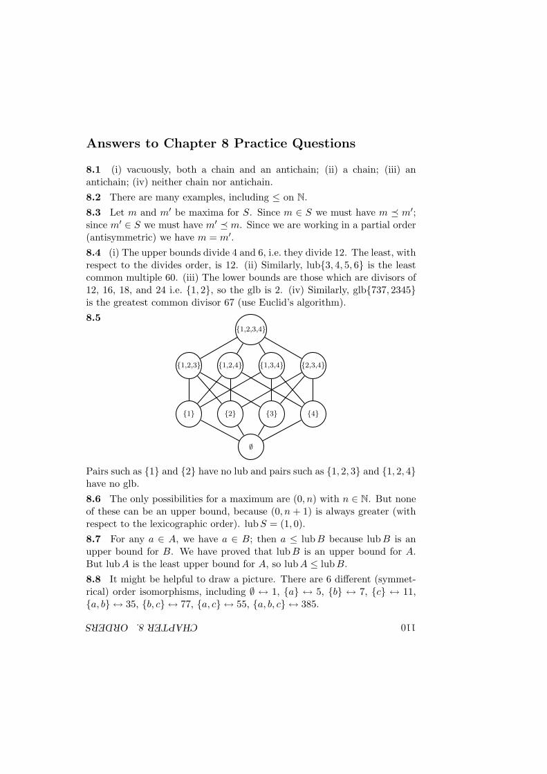
110CHAPTER8.ORDERSAnswers to Chapter 8 Practice Questions
8.1 (i) vacuously, both a chain and an antichain; (ii) a chain; (iii) anantichain; (iv) neither chain nor antichain.
8.2 There are many examples, including ≤ on N.
8.3 Let m and m′ be maxima for S. Since m ∈ S we must have m m′;since m′ ∈ S we must have m′ m. Since we are working in a partial order(antisymmetric) we have m = m′.
8.4 (i) The upper bounds divide 4 and 6, i.e. they divide 12. The least, withrespect to the divides order, is 12. (ii) Similarly, lub3, 4, 5, 6 is the leastcommon multiple 60. (iii) The lower bounds are those which are divisors of12, 16, 18, and 24 i.e. 1, 2, so the glb is 2. (iv) Similarly, glb737, 2345is the greatest common divisor 67 (use Euclid’s algorithm).
8.51,2,3,4
1,2,3 1,2,4 1,3,4 2,3,4
1 2 3 4
∅
Pairs such as 1 and 2 have no lub and pairs such as 1, 2, 3 and 1, 2, 4have no glb.
8.6 The only possibilities for a maximum are (0, n) with n ∈ N. But noneof these can be an upper bound, because (0, n + 1) is always greater (withrespect to the lexicographic order). lubS = (1, 0).
8.7 For any a ∈ A, we have a ∈ B; then a ≤ lubB because lub B is anupper bound for B. We have proved that lubB is an upper bound for A.But lubA is the least upper bound for A, so lubA ≤ lubB.
8.8 It might be helpful to draw a picture. There are 6 different (symmet-rical) order isomorphisms, including ∅ ↔ 1, a ↔ 5, b ↔ 7, c ↔ 11,a, b ↔ 35, b, c ↔ 77, a, c ↔ 55, a, b, c ↔ 385.
Index
| (“divides” relation), 47|−| (absolute value), 86Ω(-) (asymptotic lower bound), 93Θ(-) (asymptotic upper and
lower bound), 93O(-) (asymptotic upper bound), 86(:) (binomial coefficients), 36nCk (binomial coefficients), 36|A| (cardinality), 12
(cartesian product), 11× (cartesian product), 10⌈−⌉ (ceiling function), 40[a, b] (closed interval), 17A (complement), 9 (composition of functions), 24 (composition of relations), 50R−1 (converse relation), 50∅ (empty set), 3≡ (equality in modular
arithmetic), 71[a] (equivalence class), 48(−)! (factorial function), 34⌊−⌋ (floor function), 40∩ (intersection), 5∈ (is an element of), 2/∈ (is not an element of), 2⊔ (join), 105⊓ (meet), 105
(fn) (notation for a whole sequence),57
(a, b) (open interval), 17⊂ (proper subset), 4R∗ (reflexive transitive closure), 51nPk (related to binomial coefficients),
36\ (relative complement), 8Z (set of integers), 3Zn (set of integers modulo n), 3N (set of natural numbers), 3N+ (set of positive integers), 3Q (set of rational numbers), 3R (set of real numbers), 3≺ (strict order), 99⊆ (subset), 4∆ (symmetric difference), 8⊕ (symmetric difference), 8R+ (transitive closure), 51∪ (union), 5, 8∑n
i=m ai (sum of sequencesegment), 61
f : A → B (function domainand codomain), 18
f : a 7→ b (function map), 18
1-1, 20
absolute value, 86additive inverse, 72
111
112 INDEX
algebraic laws, 5antichain, 98antisymmetric, 47arrangement, 34arrow, 52associative, 24, 26associativity, 5
bag, 12base case, 59Bell numbers, 63big-O notation, 86big-Omega notation, 93big-Theta notation, 93bijection, 20bijective, 20binary operator, 26binomial coefficients, 35binomial theorem, 65boundary condition, 58bounded, 87bounded above, 103braces, 2
cancellation, 9cardinality, 12cartesian product, 10ceiling, 40chain, 98, 99characteristic polynomial, 65closed interval, 18codomain, 18combination, 35combinatorial coefficients, 35commutative, 24, 26commutativity, 5comparable, 98complement, 9
complete lattice, 105component, 10composition (of functions), 24composition (of relations), 50contrapositive, 21converse relation, 50coprime, 75counterexample, 14cover relation, 101
data compression, 78De Morgan’s laws, 9derangement, 39, 62digraph, 52directed graph, 52disjoint, 5distributivity, 5, 10div, 74divides relation, 47Dobinski’s formula, 64domain, 18dominated, 103double inclusion proof, 4
edge, 52element, 2, 10empty set, 3enumerative combinatorics, 31equality (of functions), 19equality (of sets), 4equivalence class, 48equivalence relation, 48Euclid’s algorithm, 76Euclid’s theorem, 76exclusive, 32
factorial, 34, 89Fibonacci sequence, 58
INDEX 113
floor, 40function, 18function on A, 18
generating function, 67glb, 104greatest common divisor (gcd), 75greatest lower bound, 104
half-open interval, 18Hasse diagram, 101homogeneous, 65
idempotence, 5idempotent, 26identity element, 26identity function, 19if and only if, 7image, 20inclusion-exclusion principle, 38, 39incomparable, 98independent, 33indexing set, 8induction, 59inductive hypothesis, 59inductive step, 59infimum, 104infix, 26, 46inhomogeneous, 66injection, 20injective, 20integers, 3integers modulo n, 3, 71intersection, 5, 8interval, 17interval property, 17inverse, 50inverse function, 25
involution, 9irrational, 22irreflexive, 47
join, 104
labelled digraph, 53Landau’s notation, 86lattice, 105law of product, 33law of subtract, 33law of sum, 32least upper bound, 104lemma, 89lexicographic order, 99, 102linear order, 98lossless, 78lower bound, 103lub, 104
maximum, 103meet, 104member, 2method of repeated squaring, 73minimal counterexample, 61minimum, 103mod, 74modular arithmetic, 72modulo n, 72modulus, 71monoid, 27multinomial coefficients, 41multiplicative inverse, 77
natural numbers, 3node, 52
observational equivalence, 48one, 5
114 INDEX
one-to-one map, 20onto, 20open interval, 18order, 98order isomorphism, 107ordered pair, 10
parity, 23partial function, 19partial order, 97partial sums, 62partially ordered set, 98partition, 49, 63Pascal’s triangle, 35permutation, 35pigeonhole principle, 77poset, 98positive integers, 3power set, 12prefix, 26, 98preorder, 97prime number, 75principle of induction, 59principle of strong induction, 60product order, 99, 102proof, 4proof by contradiction, 22proper subset, 4property, 31
range, 20rational numbers, 3, 22real numbers, 3recurrence relation, 58recursive, 58reduction, 72reflexive, 47reflexive transitive closure, 51
relation, 45relative complement, 8relatively prime, 75restriction, 26right-distributivity, 9RSA, 73
sequence, 57serial, 47set, 1set comprehension, 2set membership, 2Stirling’s formula, 91strict order, 99strong induction, 60subset, 4superset, 4supremum, 104surjection, 20surjective, 20symmetric, 47symmetric difference, 8
time complexity, 58total, 98total function, 19total order, 98totality, 98totally ordered set, 98transitive, 47transitive closure, 51tuple, 11
union, 5, 7universe, 9upper bound, 103
well-defined, 23words, 101

INDEX 115
zero, 5