anders w. sandvik, boston universitypeople.sissa.it/~becca/scuolaqmc/sandvik1.pdf · anders w....
TRANSCRIPT

Quantum Monte Carlo Methods at Work for Novel Phases of MatterTrieste, Italy, Jan 23 - Feb 3, 2012
Anders W. Sandvik, Boston University
Lecture 1Stochastic Series Expansion Algorithmsfor Quantum Spin SystemsLecture 2Ground State Projector Monte Carlo and the Valence Bond Basis for S=1/2 Systems
Review article on quantum spin systemsArXiv:1101.3281
Lecture 3Quantum Monte Carlo simulations of “deconfined” quantum criticality
1Sunday, January 29, 12

TutorialsPrograms and instructions available at
http://physics.bu.edu/~sandvik/trieste12/
Quantum Monte Carlo Methods at Work for Novel Phases of MatterTrieste, Italy, Jan 23 - Feb 3, 2012
Instructor: Ying Tang, Boston University
Day 1SSE code for 1D and 2D S=1/2 Heisenberg model• become familiar with programs and how to use them• do some runs and test finite-size scaling behavior• make a small addition to the program and test it
Day 2Ground state projector Monte Carlo code for1D and 2D S=1/2 Heisenberg model and 1D J-Q chain• become familiar with programs and how to use them• check convergence and compare with SSE (Heisenberg)• Investigate valence-bond-solid in J-Q chain
2Sunday, January 29, 12

Introduction: Why study quantum spin systems?Solid-state physics• localized electronic spins in Mott insulators (e.g., high-Tc cuprates)• large variety of lattices, interactions, physical properties• search for “exotic” quantum states in such systems (e.g., spin liquid)Ultracold atoms (in optical lattices)• some spin hamiltonians can be engineered (ongoing efforts)• some bosonic systems very similar to spins (e.g., “hard-core” bosons)Quantum information theory / quantum computing• possible physical realizations of quantum computers using interacting spins• many concepts developed using spins (e.g., entanglement)
Generic quantum many-body physics• testing grounds for collective quantum behavior, quantum phase transitions• identify “Ising models” of quantum many-body physics
Particle physics / field theory / quantum gravity• some quantum-spin phenomena have parallels in high-energy physics
• e.g., spinon confinement-deconfinement transition• spin foams, string nets: models to describe “emergence” of space-time and
elementary particles3Sunday, January 29, 12

H = �t�
⇤i,j⌅
�
�=�,⇥c+i,�cj,� + U
�
i
ni,�ni,⇥ = Ht + HU
U>>t : use degenerate perturbation theory (e.g., Schiff)
Mott insulators; origins of the Heisenberg antiferromagnetHubbard model (half-filling; one electron per site)
Exchange mechanism
Treat Ht as a perturbation to the ground states of HU• U=∞, one particle on every site; 2N degenerate spin states• degeneracy lifted in order t2/U - 1 doubly-occupied site, d=1• leads to the Heisenberg model
• =⇤ � =⌅
He�mn =
�
i
⇥n|Ht|i⇤⇥i|Ht|m⇤E0 � Ei
|i� : d = 1|m�, |n� : d = 0
� U
H = J�
⇥ij⇤
⌅Si · ⌅Sj = J�
⇥ij⇤
[Szi Sz
j + 12 (S+
i S�j + S�
i S+j )] J =
4t2
U4Sunday, January 29, 12

Outline• Path integrals in quantum statistical mechanics• The series-expansion representation• Stochastic Series Expansion (SSE) algorithm for the Heisenberg model• The valence-bond basis for S=1/2 systems• Ground-state projector algorithm with valence bonds
Anders W. Sandvik, Boston University
Stochastic Series Expansion Algorithmsfor Quantum Spin Systems
Reference: AIP Conf. Proc. 1297, 135 (2010); arXiv:1101.3281Detailed lecture notes on quantum spin models and methods
Quantum Monte Carlo Methods at Work for Novel Phases of MatterTrieste, Italy, Jan 23 - Feb 3, 2012
5Sunday, January 29, 12

Path integrals in quantum statistical mechanics
⇤A⌅ =1Z
Tr{Ae��H}
We want to compute a thermal expectation value
where β=1/T (and possibly T→0). How to deal with the exponential operator?
Z =�
�0
�
�1
· · ·�
�L�1
⇥�0|e��� H |�L�1⇤ · · · ⇥�2|e��� H |�1⇤⇥�1|e��� H |�0⇤
Choose a basis and insert complete sets of states;
Z = Tr{e��H} = Tr
�L⇤
l=1
e��� H
⇥“Time slicing” of the partition function
�� = �/L
Z ⇤�
{�}
⌅�0|1��⇥H|�L�1⇧ · · · ⌅�2|1��⇥H|�1⇧⌅�1|1��⇥H|�0⇧
Use approximation for imaginary time evolution operator. Simplest way
Leads to error . Limit can be taken �� � 0� ��
6Sunday, January 29, 12
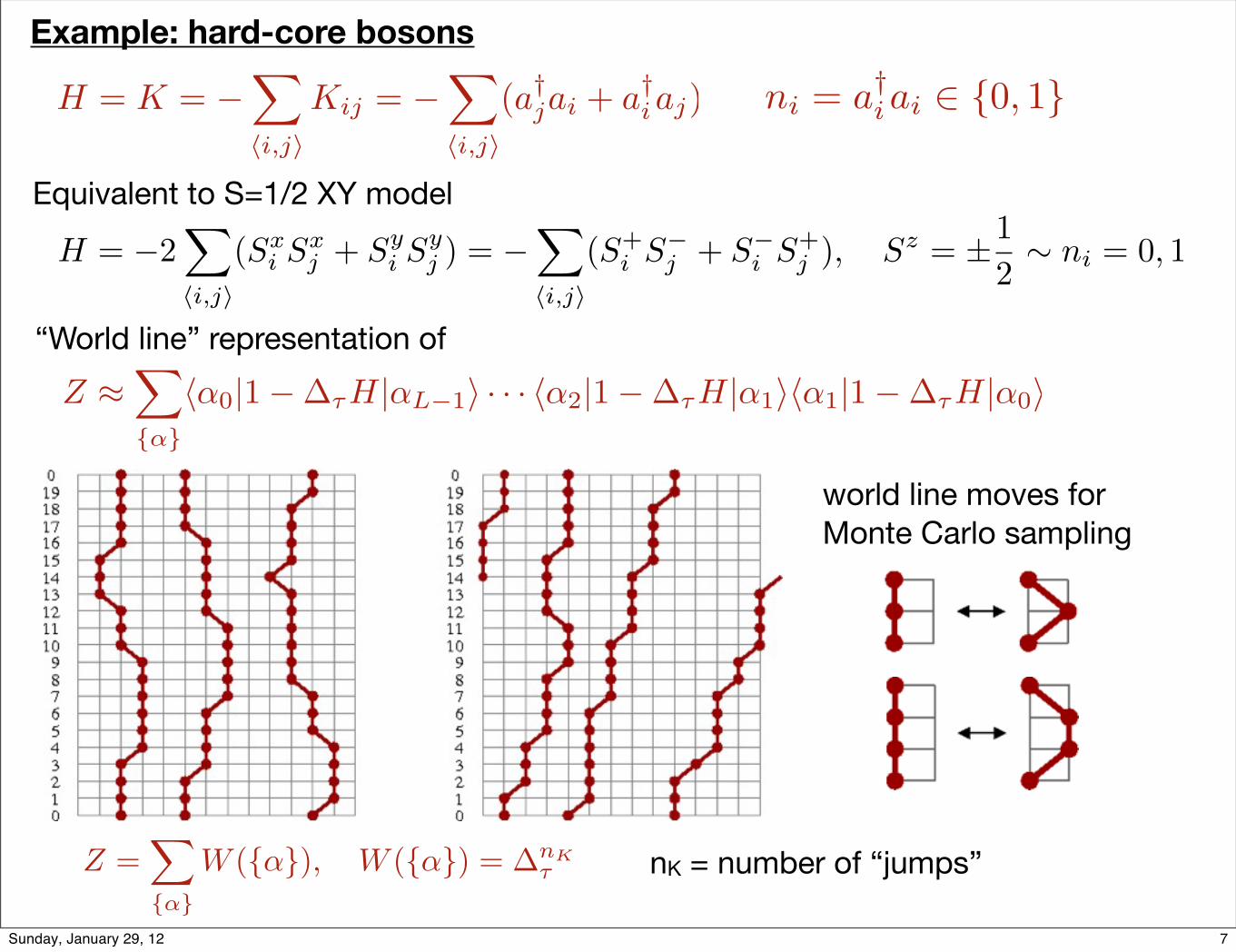
Example: hard-core bosons
H = K = ��
�i,j⇥
Kij = ��
�i,j⇥
(a†jai + a†iaj) ni = a†iai � {0, 1}
Equivalent to S=1/2 XY model H = �2
�
⇥i,j⇤
(Sxi Sx
j + Syi Sy
j ) = ��
⇥i,j⇤
(S+i S�
j + S�i S+
j ), Sz = ±12⇤ ni = 0, 1
world line moves for Monte Carlo sampling
“World line” representation of
Z =�
{�}
W ({�}), W ({�}) = �nK⇥ nK = number of “jumps”
Z ⇤�
{�}
⌅�0|1��⇥H|�L�1⇧ · · · ⌅�2|1��⇥H|�1⇧⌅�1|1��⇥H|�0⇧
7Sunday, January 29, 12

⇥A⇤ =1Z
�
{�}
⇥�0|e��� |�L�1⇤ · · · ⇥�2|e��� H |�1⇤⇥�1|e��� HA|�0⇤
Expectation values
⇧A⌃ =
�{�} A({�})W ({�})�
{�} W ({�}) �⇥ ⇧A⌃ = ⇧A({�})⌃W
We want to write this in a form suitable for MC importance sampling
W ({�}) = weightA({�}) = estimatorFor any quantity diagonal in the
occupation numbers (spin z):
A({�}) = A(�n) or A({�}) =1L
L�1�
l=0
A(�l)
There should be of the order βN “jumps” (regardless of approximation used)
Kinetic energy (here full energy). Use
Ke��� K � K101
Kij({�}) =⇧�1|Kij |�0⌃
⇧�1|1 ���K|�0⌃⇥ {0,
1��
}
Average over all slices → count number of kinetic jumps
⇤K⌅ ⇥ N � ⇤nK⌅ ⇥ �N⇥Kij⇤ =⇥nij⇤
�, ⇥K⇤ = �⇥nK⇤
�
8Sunday, January 29, 12

Including interactionsFor any diagonal interaction V (Trotter, or split-operator, approximation)
e��� H = e��� Ke��� V + O(�2� ) ⇥ ⌅�l+1|e��� H |�l⇧ � e��� Vl⌅�l+1|e��� K |�l⇧
Product over all times slices →
W ({�}) = �nK� exp
����
L�1⇤
l=0
Vl
⇥
local updates (problem when Δτ→0?)•consider probability of inserting/removing
events within a time window
The continuous time limitLimit Δτ→0: number of kinetic jumps remains finite, store events only
Special methods (loopand worm updates)developed for efficientsampling of the pathsin the continuum
⇐ Evertz, Lana, Marcu (1993), Prokofev et al (1996) Beard & Wiese (1996)
Pacc = min⇤�2
�exp��Vnew
Vold
⇥, 1
⌅
9Sunday, January 29, 12

e��H =⇥�
n=0
(��)n
n!Hn
Similar to the path integral; and weight factor outside 1���H ⇥ H
Z =⇥�
n=0
(�⇥)n
n!
�
{�}n
⇤�0|H|�n�1⌅ · · · ⇤�2|H|�1⌅⇤�1|H|�0⌅
Series expansion representation
Start from the Taylor expansion
For hard-core bosons the (allowed) path weight is W ({�}n) = ⇥n/n!
C = ⇥n2⇤ � ⇥n⇤2 � ⇥n⇤
From this follows: narrow n-distribution with ⇥n⇤ � N�, ⇥n ��
N�
(approximation-freemethod from the outset)
For any model, the energy is
one more “slice” to sum over here
relabel terms to “get rid of” extra slice
E =1Z
⇥�
n=0
(�⇥)n
n!
�
{�}n+1
⇤�0|H|�n⌅ · · · ⇤�2|H|�1⌅⇤�1|H|�0⌅
= � 1Z
⇥�
n=1
(�⇥)n
n!n
⇥
�
{�}n
⇤�0|H|�n�1⌅ · · · ⇤�2|H|�1⌅⇤�1|H|�0⌅ =⇤n⌅⇥
this is the operator we “measure”
�
10Sunday, January 29, 12

Fixed-length scheme• n fluctuating → varying size of the configurations• the expansion can be truncated at some nmax=L (exponentially small error)• cutt-off at n=L, fill in operator string with unit operators H0=I
Here n is the number of Hi, i>0 instances in the sequence of L operators
Z =�
{�}L
�
{Hi}
(�⇥)n(L � n)!L!
⇤�0|Hi(L)|�L�1⌅ · · · ⇤�2|Hi(2)|�1⌅⇤�1|Hi(1)|�0⌅
�L
n
⇥�1
=n!(L� n)!
L!
- conisider all possible locations in the sequence- overcounting of actual (original) strings, correct by combinatorial factor:
=�
11Sunday, January 29, 12

Stochastic Series expansion (SSE): S=1/2 Heisenberg modelWrite H as a bond sum for arbitrary lattice
H = JNb�
b=1
Si(b) · Sj(b),
H1,b = 14 � Sz
i(b)Szj(b),
H2,b = 12 (S+
i(b)S�j(b) + S�i(b)S
+j(b)).
Diagonal (1) and off-diagonal (2) bond operators
H = �JNb�
b=1
(H1,b �H2,b) +JNb
4
⇤�i(b)⇥j(b) |H1,b| �i(b)⇥j(b)⌅ = 12 ⇤⇥i(b)�j(b) |H2,b| �i(b)⇥j(b)⌅ = 1
2
⇤⇥i(b)�j(b) |H1,b| ⇥i(b)�j(b)⌅ = 12 ⇤�i(b)⇥j(b) |H2,b| ⇥i(b)�j(b)⌅ = 1
2
Four non-zero matrix elements
2D square latticebond and site labels
Z =⌅
�
⇥⌅
n=0
(�1)n2⇥n
n!
⌅
Sn
⇥�
�����
n�1⇧
p=0
Ha(p),b(p)
����� �
⇤Partition function
Sn = [a(0), b(0)], [a(1), b(1)], . . . , [a(n� 1), b(n� 1)]Index sequence:
n2 = number of a(i)=2(off-diagonal operators)in the sequence
12Sunday, January 29, 12

Propagated states: |�(p)⇥ �p�1�
i=0
Ha(i),b(i) |�⇥
For fixed-length scheme
W (�, SL) =�
⇥
2
⇥n (L� n)!L!
In a program:
s(p) = operator-index string• s(p) = 2*b(p) + a(p)-1• diagonal; s(p) = even• off-diagonal; s(p) = off
σ(i) = spin state, i=1,...,N• only one has to be stored
W>0 (n2 even) for bipartite lattice Frustration leads to sign problem
SSE effectively provides a discrete representation of the time continuum • computational advantage; only integer operations in sampling
Z =⌅
�
⌅
SL
(�1)n2⇥n(L� n)!
L!
⇥�
�����
L�1⇧
p=0
Ha(p),b(p)
����� �
⇤
13Sunday, January 29, 12

Linked vertex storage
0 1
2 3
0 1
2 3
0 1
2 3
0 1
2 3
The “legs” of a vertex represents the spin states before (below) and after (above) an operator has acted
X( ) = vertex list• operator at p→X(v) v=4p+l, l=0,1,2,3• links to next and previous leg
Spin states between operations are redundant; represented by links• network of linked vertices will be used for loop updates of vertices/operators
14Sunday, January 29, 12

Monte Carlo sampling scheme
Change the configuration; (�, SL)� (��, S�L)
Attempt at p=0,...,L-1. Need to know |α(p)>• generate by flipping spins when off-diagonal operator
Diagonal update: [0, 0]p � [1, b]p
W (�, SL) =�
⇥
2
⇥n (L� n)!L!
Paccept([0, 0]⇥ [1, b]) = min�
�Nb
2(L� n), 1
⇥
Paccept([1, b]⇥ [0, 0]) = min�2(L� n + 1)
�Nb, 1
⇥
Acceptance probabilities
W (a = 0)W (a = 1)
=L� n + 1
�/2W (a = 1)W (a = 0)
=�/2
L� n
n is the current power• n → n+1 (a=0 → a=1)• n → n-1 (a=1 → a=0)
Pselect(a = 0� a = 1) = 1/Nb, (b ⇥ {1, . . . , Nb})Pselect(a = 1� a = 0) = 1
Paccept = min�W (��, SL)W (�, SL)
Pselect(��, S�L � �, SL)
Pselect(�, SL � ��, S�L)
, 1⇥
15Sunday, January 29, 12
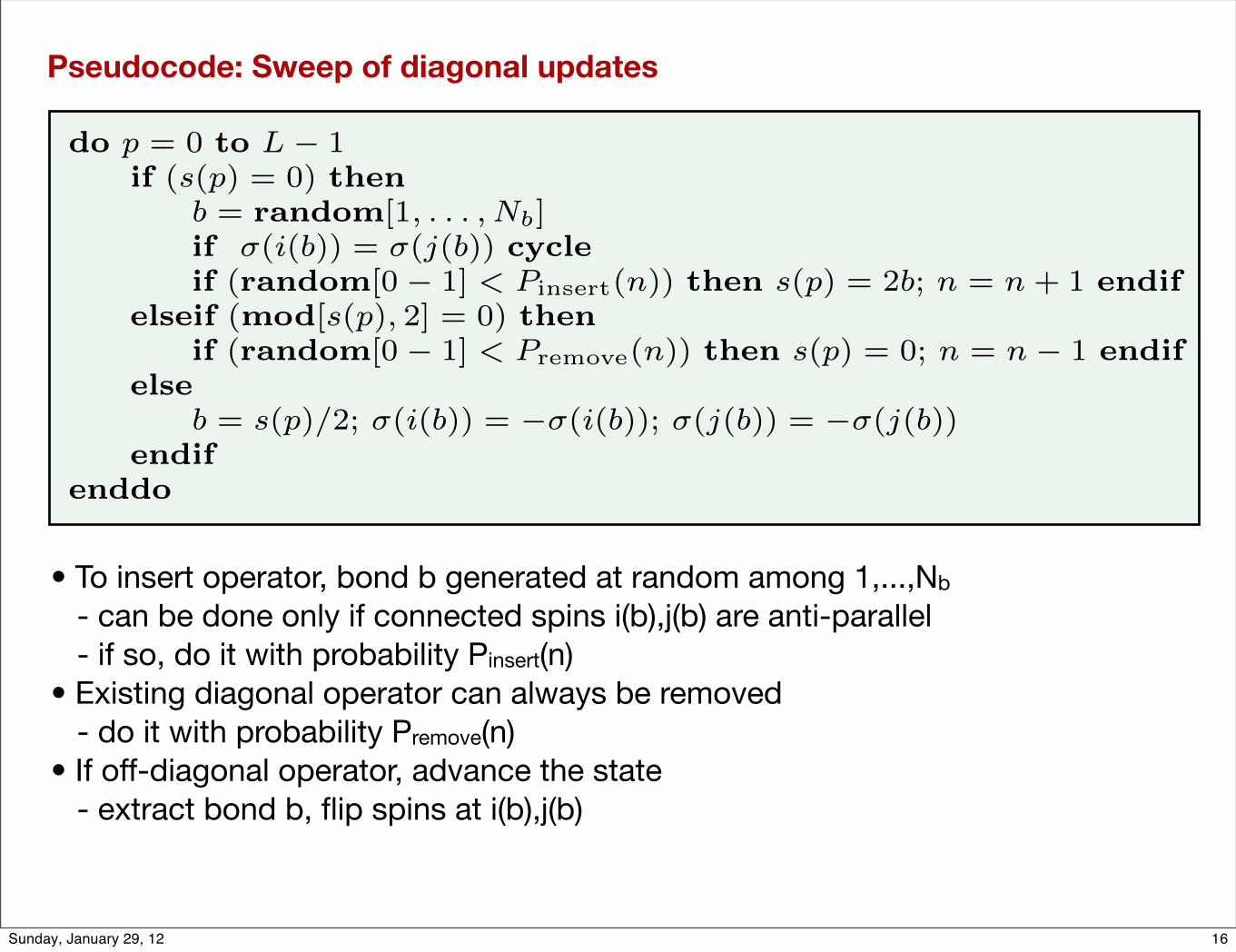
do p = 0 to L � 1if (s(p) = 0) then
b = random[1, . . . , Nb]if �(i(b)) = �(j(b)) cycle
if (random[0 � 1] < Pinsert
(n)) then s(p) = 2b; n = n + 1 endif
elseif (mod[s(p), 2] = 0) then
if (random[0 � 1] < Premove
(n)) then s(p) = 0; n = n � 1 endif
else
b = s(p)/2; �(i(b)) = ��(i(b)); �(j(b)) = ��(j(b))endif
enddo
Pseudocode: Sweep of diagonal updates
• To insert operator, bond b generated at random among 1,...,Nb - can be done only if connected spins i(b),j(b) are anti-parallel - if so, do it with probability Pinsert(n)• Existing diagonal operator can always be removed - do it with probability Premove(n)• If off-diagonal operator, advance the state - extract bond b, flip spins at i(b),j(b)
16Sunday, January 29, 12

Off-diagonal updates
Operator-loop update• Many spins
and operators can be changed simultaneously
• can change winding numbers
Local updateChange the typeof two operators• constraints• inefficient• cannot change
winding numbers
17Sunday, January 29, 12

do v0 = 0 to 4L� 1 step 2if (X(v0) < 0) cyclev = v0if (random[0� 1] < 1
2 ) thentraverse the loop; for all v in loop, set X(v) = �1
elsetraverse the loop; for all v in loop, set X(v) = �2flip the operators in the loop
endifenddo
constructing all loops, flip probability 1/2
construct and flip a loop
v = v0do
X(v) = �2p = v/4; s(p) = flipbit(s(p), 0)v� = flipbit(v, 0)v = X(v�); X(v�) = �2if (v = v0) exit
enddo
Pseudocode: Sweep of loop updates
• by flipping bit 0 of s(p), the operator changes from diagonal to off-diagonal, or vise versa
18Sunday, January 29, 12

We also have to modify the stored spin state after the loop update• we can use the information in Vfirst() and X() to determine spins to be flipped• spins with no operators, Vfirst(i)=−1, flipped with probability 1/2
do i = 1 to Nv = Vfirst(i)if (v = �1) then
if (random[0-1]< 1/2) �(i) = ��(i)else
if (X(v) = �2) �(i) = ��(i)endif
enddo
v=Vfirst(i) is the location of the first vertex leg on site i• flip the spin if X(v)=−2• (do not flip it if X(v)=−1)• no operation on i if vfirst(i)=−1; then it is flipped with probability 1/2
19Sunday, January 29, 12

Vfirst(:) = �1; Vlast(:) = �1do p = 0 to L� 1
if (s(p) = 0) cyclev0 = 4p; b = s(p)/2; s1 = i(b); s2 = j(b)v1 = Vlast(s1); v2 = Vlast(s2)if (v1 ⇥= �1) then X(v1) = v0; X(v0) = v1 else Vfirst(s1) = v0 endifif (v2 ⇥= �1) then X(v2) = v0; X(v0) = v2 else Vfirst(s2) = v0 + 1 endifVlast(s1) = v0 + 2; Vlast(s2) = v0 + 3
enddo
Constructing the linked vertex list
creating the last links across the “time” boundarydo i = 1 to N
f = Vfirst(i)if (f ⇥= �1) then l = Vlast(i); X(f) = l; X(l) = f endif
enddo
Use arrays to keep track of the first and last (previous) vertex leg on a given spin• Vfirst(i) = location v of first leg on site i• Vlast(i) = location v of last (currently) leg• these are used to create the links• initialize all elements to −1
Traverse operator list s(p), p=0,...,L−1• vertex legs v=4p,4p+1,4p+2,4p+3
20Sunday, January 29, 12

Determination of the cut-off L• adjust during equilibration• start with arbitrary (small) n
Keep track of number of operators n• increase L if n is close to current L• e.g., L=n+n/3
Example •16×16 system, β=16 ⇒• evolution of L• n distribution after equilibration
• truncation is no approximation
21Sunday, January 29, 12

Does it work?Compare with exact results• 4×4 exact diagonalization• Bethe Ansatz; long chains
⇐ Energy for long 1D chains• SSE results for 106 sweeps• Bethe Ansatz ground state E/N• SSE can achieve the ground state limit (T→0)
Susceptibility of the 4×4 lattice ⇒• SSE results from 1010 sweeps• improved estimator gives smaller error bars at high T (where the number of loops is larger)
22Sunday, January 29, 12