Optimized Effective Potentialand the electrical response of finite systems

Stephan Kummel

Max-Planck-Institut fur Physik komplexer Systeme, Dresden

Emmy Noether-Programm der DFG

Orbital Functionals for Exchange and Correlation, Berlin, March 11, 2005

OEP and response – p.1

Outline

1. Ground-state DFT1.1. Calculating the Optimized Effective Potential

using orbitals and orbital shifts

1.2. Electrical response of molecular chainswhy exact OEP makes a difference: potential barriers and derivativediscontinuity

2. Time-dependent DFT2.1. Strong-field double ionization of Helium

a paradigm problem

2.2. Exact time-dependent correlation potentials“adiabatic thinking” and the derivative discontinuity again

3. Conclusion

OEP and response – p.2

0. Optimized Effective Potential – why?

(Semi)local functionals o.k. for ground-state properties but have wellknown problems (e.g., dissociation, charge transfer, localization, excitations, ...)

How to drive out the self-interaction error?

Orbital functionals can be a way – e.g., by incorporating exactexchange:

Eexx = −e

2

2

∑

σ=↑,↓

Nσ∑

i,j=1

∫ ∫ϕ∗iσ(r)ϕ∗jσ(r′)ϕjσ(r)ϕiσ(r′)

|r− r′| d3r′ d3r

Kohn-Sham ϕiσ from common local potential, i.e., Eex,KSx 6= EHF

x

But:problem 1: Eloc

xc rely on “cancellation of errors” in E locx and Eloc

c

problem 2: vlocxc (r) =

δElocxc [n]δn(r) = ... o.k., but vex

x (r) =δEex

x [{ϕi}]δn(r) = ... ?

OEP and response – p.3

1.1 Calculating the OEP from orbital shifts

vxcσ(r) =δExc [{ϕjτ}]δnσ(r)

=

Nα∑

i=1α=↑,↓

∫δExc [{ϕjτ}]δϕiα(r′)

δϕiα(r′)δnσ(r)

d3r′ + c.c. = ...

Nσ∑

i=1

∫ϕ∗iσ(r′) [vxcσ(r′)− uxciσ(r′)]

∞∑

j=1j 6=i

ϕjσ(r′)ϕ∗jσ(r)

εiσ − εjσd3r′ϕiσ(r) + c.c. = 0

Optimized Effective Potential (OEP) integral equation

where uxciσ(r) = 1ϕ∗iσ(r)

δExc[{ϕjτ}]δϕiσ(r)

Note OEP short form:∑Nσ

i=1 ψ∗iσ(r)ϕiσ(r) + c.c. = 0

Talman, Shadwick (1976) Krieger, Li, Iafrate (1992) Engel (1993) Kotani, Akai (1996) Kurth, Gross (1997)

Görling, Levy (1999) Ivanov, Bartlett (1999) Gritsenko, Baerends (2001) Yang, Wu (2002)

OEP and response – p.4

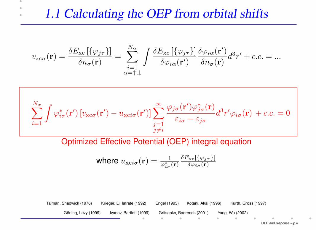
1.1 Calculating the OEP from orbital shifts

vxcσ(r) =δExc [{ϕjτ}]δnσ(r)

=

Nα∑

i=1α=↑,↓

∫δExc [{ϕjτ}]δϕiα(r′)

δϕiα(r′)δnσ(r)

d3r′ + c.c. = ...

Nσ∑

i=1

∫ϕ∗iσ(r′) [vxcσ(r′)− uxciσ(r′)]

∞∑

j=1j 6=i

ϕjσ(r′)ϕ∗jσ(r)

εiσ − εjσd3r′ϕiσ(r) + c.c. = 0

Optimized Effective Potential (OEP) integral equation

where uxciσ(r) = 1ϕ∗iσ(r)

δExc[{ϕjτ}]δϕiσ(r)

Note OEP short form:∑Nσ

i=1 ψ∗iσ(r)ϕiσ(r) + c.c. = 0

Talman, Shadwick (1976) Krieger, Li, Iafrate (1992) Engel (1993) Kotani, Akai (1996) Kurth, Gross (1997)

Görling, Levy (1999) Ivanov, Bartlett (1999) Gritsenko, Baerends (2001) Yang, Wu (2002)

OEP and response – p.4

Iterative OEP construction

Explicit expression for vxc(r):

vxcσ(r) =1

2nσ(r)

Nσ∑

i=1

{|ϕiσ(r)|2 [uxciσ(r) + (vxciσ − uxciσ)]

−~2

m∇ · (ψ∗iσ(r)∇ϕiσ(r))

}+ c.c.

where vxciσ = 〈ϕiσ| vxcσ |ϕiσ〉, uxciσ = 〈ϕiσ|uxciσ |ϕiσ〉KLI-approximation: ψiσ(r) = 0∀ i

Coupled equations for ϕiσ(r) and ψiσ(r): i=1,...,Nσ

(hKSσ − εiσ)ϕiσ(r) = 0

(hKSσ − εiσ)ψ∗iσ(r) = −[vxcσ(r)− uxciσ(r)− (vxciσ − uxciσ)]ϕ∗iσ(r)

where hKSσ = − ~2

2m∇2 + vext(r) + vH(r) + vxcσ(r)

S. K. and J. P. Perdew, Phys. Rev. Lett. 90, 043004 (2003); Phys. Rev. B 68, 035103 (2003)

OEP and response – p.5

1.2 Electrical response of molecular chains

Linear and nonlinear electrical response of PA

C C

C C

C

C

C

C

H H H

H H H

H

H

alternating bondlengths

high electron mobility along the backbone of the chain, verylittle transverse

large and directional linear and nonlinearresponse/polarizability

interesting for non-linear optical devices

theory: understanding why properties are as observed,guidance in search for improvements

many electrons, thus DFT would be method of choice but...

OEP and response – p.6

Failure of (semi)local approximations

Linear and nonlinear response

linear polarizability: α= ∂2E∂F2

∣∣∣F=0

=∂µ∂F

∣∣∣F=0

electrical field F, energy E, dipolemoment µz = −eRn(r,F)z d3r

second hyperpolarizability: γ= ∂4E∂F4

∣∣∣F=0

=∂3µ∂F3

∣∣∣F=0

Problem:LDA, GGAs: large errors in linear, huge errors in nonlinear

polarizability

C20H22: αLDA ≈ 2× αC44H46: γLDA ≈ 60× γ

along backbone

B. Champagne et al., J. Chem. Phys. 109, 10489 (1998)

OEP and response – p.7

Analyzing the problem

Hydrogen chain

H H H H H H H H

“mimic” PA, but technically more transparent, CC possible

polarizability problems as in PA:H12: αLDA ≈ 2× αH18: γLDA ≈ 11× γ

Hartree-Fock is accurate for response, x-KLI not!

Example H12: γLDA ≈ 8× γHF, γxKLI ≈ 2× γHF

S. J. A. van Gisbergen et al., Phys. Rev. Lett. 83, 694 (1999)

Option 1: HF-x intrinsically superior to KS-x

Option 2: KLI much worse for response than for E

OEP and response – p.8

Analyzing the problem

Hydrogen chain

H H H H H H H H

“mimic” PA, but technically more transparent, CC possible

polarizability problems as in PA:H12: αLDA ≈ 2× αH18: γLDA ≈ 11× γ

Hartree-Fock is accurate for response, x-KLI not!

Example H12: γLDA ≈ 8× γHF, γxKLI ≈ 2× γHF

S. J. A. van Gisbergen et al., Phys. Rev. Lett. 83, 694 (1999)

Option 1: HF-x intrinsically superior to KS-x

Option 2: KLI much worse for response than for E

OEP and response – p.8

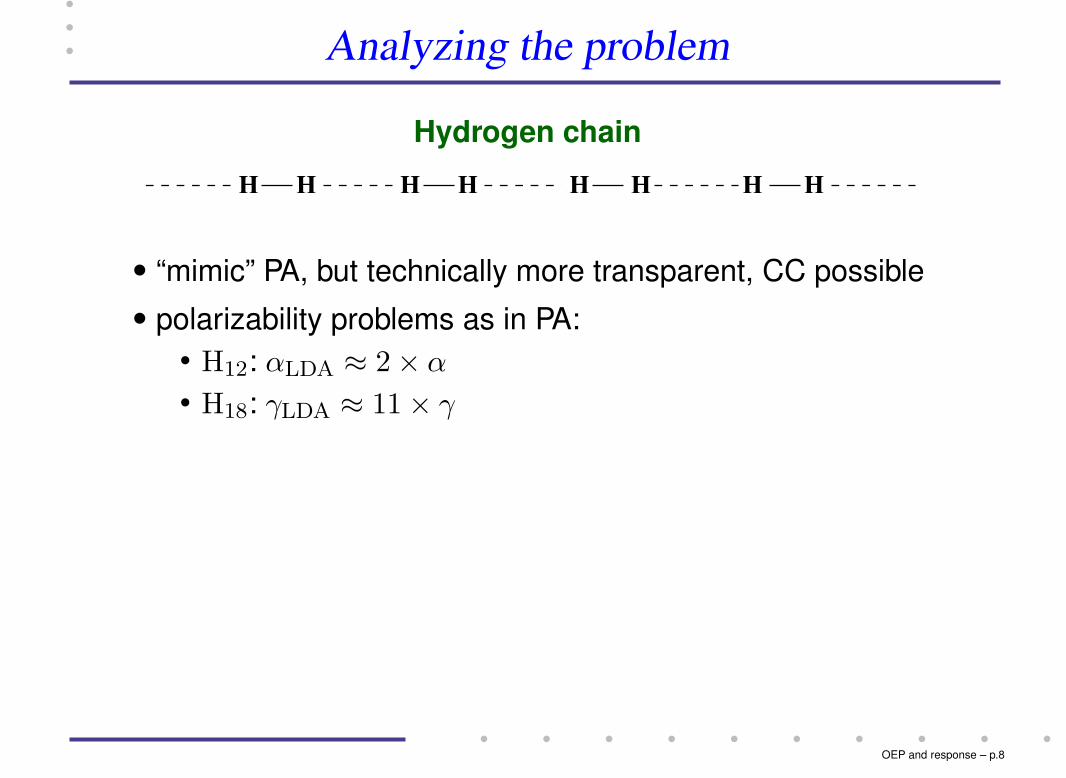
Analyzing the problem

Hydrogen chain

H H H H H H H H

“mimic” PA, but technically more transparent, CC possible

polarizability problems as in PA:H12: αLDA ≈ 2× αH18: γLDA ≈ 11× γ

Hartree-Fock is accurate for response, x-KLI not!

Example H12: γLDA ≈ 8× γHF, γxKLI ≈ 2× γHF

S. J. A. van Gisbergen et al., Phys. Rev. Lett. 83, 694 (1999)

Option 1: HF-x intrinsically superior to KS-x

Option 2: KLI much worse for response than for E

OEP and response – p.8

Response from true OEP

Fundamental problem? Check x-OEP response!

hyperpolarizabilities tedious to calculate

α γ/103

H6 H12 H6 H12

LDA 72.2 210.5 101 1200KLI 60.2 156.3 36 300

OEP 56.6 138.1 30 144HF 56.4 137.6 30 147

in atomic units

DFT with x-OEP close to HF – no KS-x problem!

Error in KLI-approximation (H12): E: 0.03% γ: 100% !Why?

Exact exchange very different from LDA – Why?

S. K., L. Kronik, and J. P. Perdew, Phys. Rev. Lett. 93, 213002 (2004)

OEP and response – p.9

Response from true OEP

Fundamental problem? Check x-OEP response!

hyperpolarizabilities tedious to calculate

α γ/103

H6 H12 H6 H12

LDA 72.2 210.5 101 1200KLI 60.2 156.3 36 300

OEP 56.6 138.1 30 144HF 56.4 137.6 30 147

in atomic units

DFT with x-OEP close to HF – no KS-x problem!

Error in KLI-approximation (H12): E: 0.03% γ: 100% !Why?

Exact exchange very different from LDA – Why?S. K., L. Kronik, and J. P. Perdew, Phys. Rev. Lett. 93, 213002 (2004)

OEP and response – p.9

Exact exchange – qualitatively different

-0.8

-0.7

-0.6

-0.5

-0.4

-0.3

-0.2

-10 -5 0 5 10

v x(z

) (ha

rtree

)

z (a0)

x-KLI

x-OEP

o o o o o o o o

0

0.05

0.1

0.15

0.2

0.25

-10 -5 0 5 10

n(z)

(a0-3

)

z (a0)

o o o o o o o o

KLI underestimates barriersin low-density regions→ little influence on E,

large on response

LDA works with the externalfield, exact x against it

-0.03

-0.02

-0.01

0

0.01

0.02

0.03

-10 -5 0 5 10

v F=0

.005

(z)-

v F=0

(z)

z (a0)

x-OEP

LDA

externo o o o o o o o

OEP and response – p.10

Exact exchange – qualitatively different

-0.8

-0.7

-0.6

-0.5

-0.4

-0.3

-0.2

-10 -5 0 5 10

v x(z

) (ha

rtree

)

z (a0)

x-KLI

x-OEP

o o o o o o o o

0

0.05

0.1

0.15

0.2

0.25

-10 -5 0 5 10

n(z)

(a0-3

)

z (a0)

o o o o o o o o

KLI underestimates barriersin low-density regions→ little influence on E,

large on response

LDA works with the externalfield, exact x against it

-0.03

-0.02

-0.01

0

0.01

0.02

0.03

-10 -5 0 5 10

v F=0

.005

(z)-

v F=0

(z)

z (a0)

x-OEP

LDA

externo o o o o o o o

OEP and response – p.10

Derivative discontinuity→ counteracting field

Known: vxc(r) changes discontinuously at integer NJ. P. Perdew, R. G. Parr, M. Levy, and J. L. Balduz, Jr., Phys. Rev. Lett. 49, 1691 (1982)

∆xc =δExc[n]

δn(r)

∣∣∣∣N+ε

− δExc[n]

δn(r)

∣∣∣∣N−ε

= C > 0

Add fraction of an electron to integer system→ vxc(r) jumps up

-2

-1.5

-1

-0.5

0

0.5

-30 -20 -10 0 10 20 30

v x (R

yd)

R (a0)

H2+ε H2-ε

Orbital functionalsshow a derivativediscontinuity, (semi)local functionals not!

OEP and response – p.11

2. Time-dependent DFT

Strong-field double ionization of He: a paradigm problem

Walker et al., Phys. Rev. Lett. 73, 1227 (1994)

Experiment:

Double ionization probabilityorders of magnitude largerthan expected fromsequential process

He2+ and He+ signals satura-te at same intensity; “knee”

Electron interaction/correlation isessential!

Mechanism: recollision process

OEP and response – p.12

He double ionzation and TDDFT

The problem:TDDFT allows to calculate non-perturbative excitations atmoderate computational costs

but “standard” approximations (ALDA, SIC, ...) do not at allreproduce the He “knee”

→ failure for paradigm test case

M. Petersilka and E. K. U. Gross, Laser Phys. 9, 105 (1999)

OEP and response – p.13

TDDFT – formal framework

1. Runge-Gross Theorem: E. Runge and E. K. U. Gross, Phys. Rev. Lett. 52, 997 (1984)

n(r, t) determines the external potential uniquely ( up to c(t) )

⇒ every observable is an unique functional of the density

2. Time-dependent Kohn-Sham equations:Density can be obtained from single-particle orbitals ϕk(r, t)

n(r, t) =∑N

k=1 |ϕk(r, t)|2

i~ ∂∂tϕk(r, t) =(− ~2

2m∇2 + vs(r, t))ϕk(r, t)

vs(r, t) = vext(r, t) + e2∫ n(r′,t)|r−r′| + vxc[n](r, t)

Two problems: i) better approximation for vxc[n](r, t)?

ii) P1, P2 as functionals of the density?

OEP and response – p.14

Obtaining an exact vxc(r)

one-dimensional model: H(t) =

− ~2

2m∂2

∂z21− ~2

2m∂2

∂z22− 2e2√

z21+1− 2e2√

z22+1

+ e2√(z1−z2)2+1

+ eE(t)(z1 + z2)

First stage of recollision mechanism: field-induced ionization

Solve time-dependent Schrödinger equation⇒ exacttime-dependent density n(z, t) and current-density j(z, t)

Calculate time-dependent Kohn-Sham orbitalϕ(z, t) =

√n(z, t)/2 exp(iα(z, t))

from n(z, t) and js(z, t) = j(z, t)

Calculate time-dependent Kohn-Sham potential

vs(z, t) =i~ ∂ϕ∂t + ~2

2m∇2ϕ

ϕ (in practice: invert split-operator propagator)

OEP and response – p.15

Compare vc(r, t) to ground-state vc(r)

time-dependentdensity potential

ground-state with fractionaloccupation

n1+ε(z) = (1− ε)n1(z) + εn2(z),

ϕ(z) =pn1+ε(z)/(1 + ε),

vs(z) =~2

2m

1

ϕ(z)

d2ϕ(z)

dz2+ const.

Static vc(r) with fractional occupation similar to time-dependentvc(r, t)

OEP and response – p.16

Compare vc(r, t) to ground-state vc(r)

time-dependentdensity potential

ground-state with fractionaloccupation

n1+ε(z) = (1− ε)n1(z) + εn2(z),

ϕ(z) =pn1+ε(z)/(1 + ε),

vs(z) =~2

2m

1

ϕ(z)

d2ϕ(z)

dz2+ const.

Static vc(r) with fractional occupation similar to time-dependentvc(r, t)

OEP and response – p.16

Derivative discontinuity in vc(r)

vxc(r) changes discontinuously at integer NJ. P. Perdew, R. G. Parr, M. Levy, and J. L. Balduz, Jr., Phys. Rev. Lett. 49, 1691 (1982)

∆xc =δExc[n]

δn(r)

˛˛N+ε

− δExc[n]

δn(r)

˛˛N−ε

= C > 0

-10-9-8-7-6-5-4-3-2-1 0 1

0.01 0.1 1 10

v x(r

) (ha

rtree

)

r (a0)

vx Mg+

vx Mg+ +10-8

−10 0 10 20z (a.u.)

0.0

0.2

0.4

0.6

0.8

v Hxc

(a.u

.)

fractional occupationTime−dependent DFTStatic DFT with

OEP and response – p.17

New functional with “discontinuity by hand”

vc(z, t) = [c(Nb(0)/Nb(t))− 1] [vh(z, t) + vx(z, t)]

where c(x) = x/(1 + e50(x−2))

1014 1015

Laser intensity (W/cm2)

10−2

10−1

100

P1,

P2

squares: TDHF; circles: TDDFT open: P1 ; filled: P2

OEP and response – p.18

Conclusion

Orbital functionals can be qualitatively different

The derivative discontinuity and its time-dependentanalogue are important

Problems to address: improving the correlation descriptionand solving the time-dependent OEP equation

Thank you:Manfred Lein, MPI-PKS/MPI-K – Helium collaboration

Astrid de Wijn, MPI-PKS – Helium continued

Michael Mundt, MPI-PKS – time-dependent OEP poster

Leeor Kronik, Weizmann Institute

John Perdew, Tulane UniversityOEP and response – p.19