and structure learning in bayesian networks
TRANSCRIPT

Gaussian Mixture Models and Structure Learning in
Bayesian NetworksAnthony Platanios

EM Algorithm ReviewWe begin with an arbitrary choice for our parameters and iterate over the following steps, until convergence
E Step: Estimate the values of the unobserved variables using the current parameters
M Step: Use the observed variables along with our estimates of the unobserved variables from the previous E step to compute a maximum likelihood estimate for our parameters and update them
Guaranteed to find a local maximum

EM Algorithm Review
Guaranteed to find a local maximum
Given a joint distribution over observed variables and latent variables , parameterized by , we want to maximize with respect to
p(x, z | ✓) x
z ✓ p(x | ✓)✓
Choose ✓oldInitialization
p(z | x,✓old)E Step Calculate
M Step Solve✓
new= argmax
✓
Ez|x,✓old
{log p(x, z | ✓)}
Convergence If not converged, set ✓old ✓new

EM Algorithm Review
So far we have introduced EM as an algorithm for performing inference in cases where we have partially labeled data
However, EM can be used in many more cases, including having no labeled data at all
We are now going to consider one such cases as an example

Unsupervised EM ExampleLet’s consider a case with no labeled data at all
Classificatione.g., Naive Bayes
and Logistic Regression

Let’s consider a case with no labeled data at all
Classification ClusteringWe want to
learn the classes themselves
Unsupervised EM Example

Clustering
An instance of unsupervised learning
Examples• Find interesting groups of patients in a hospital, faces in photos, webpages, etc.
• Find interesting topics that different documents talk about based on word distributions (i.e., topic modeling)
A way of doing that is using mixtures of distributions

Mixture of DistributionsWe model the joint distribution of our observations using a mixture of multiple distributions — each observation comes from one of those distributions and the distributions define our clusters
Discrete (and unobserved) random variable that specifies which distribution each observation came from
p(x1, . . . ,xN ) =NY
n=1
KX
k=1
p(xn | zn)p(zn = k)
Cool Fact: That is what happens in Naive Bayes too

Gaussian Mixture Models (GMM)We assume that each observation is generated in the following way:
1. Randomly choose a Gaussian distribution according to
2. Sample the observation from that Gaussian distribution — that Gaussian distribution defines
p(zn = k)
p(xn | zn)
What does this look like and how do we formalize it?

GMM Example

GMM Formal DefinitionLet’s assume we have clusters. We define a variable indicating which cluster each observation belongs to using a one-hot vector
K
z = [0, 0, 0, . . . , 0, 1, 0, . . . , 0, 0]
if and only if our observation belongs to cluster zk = 1 k
This will be the unobserved latent variable of our model, corresponding to what used to be a class for each observation (in classification problems)

We define the joint distribution as follows
Each cluster has its own Gaussian distribution and the exponent picks the one corresponding to the cluster to which the current observation belongs
GMM Formal Definition
p(xn, zn) = p(xn | zn)p(zn)
p(xn | znk = 1) = N (xn | µk,⌃k) )
p(xn | zn) =KY
k=1
N (xn | µk,⌃k)znk

We define the joint distribution as follows
probability of the corresponding
cluster
p(xn, zn) = p(xn | zn)p(zn)
p(znk = 1) = ⇡k ) p(zn) =KY
k=1
⇡znk
k
GMM Formal Definition
because only one cluster can be
“active” at any time
KX
k=1
⇡k = 1

What does our model look like?
GMM Formal Definition
p(x | ✓) =NY
n=1
KX
k=1
⇡kN (xn | µk,⌃k)
✓ = {⇡,µ,⌃}µ
⇡
⌃
z1
x
1x
n
zn
…
…

xnµ
⇡
⌃
zn
N
The plate notation simply means that we have copies of the variables indexed by
Nn
What does our model look like?
GMM Formal Definition
p(x | ✓) =NY
n=1
KX
k=1
⇡kN (xn | µk,⌃k)
✓ = {⇡,µ,⌃}
Calculate the expected value of the cluster assignments
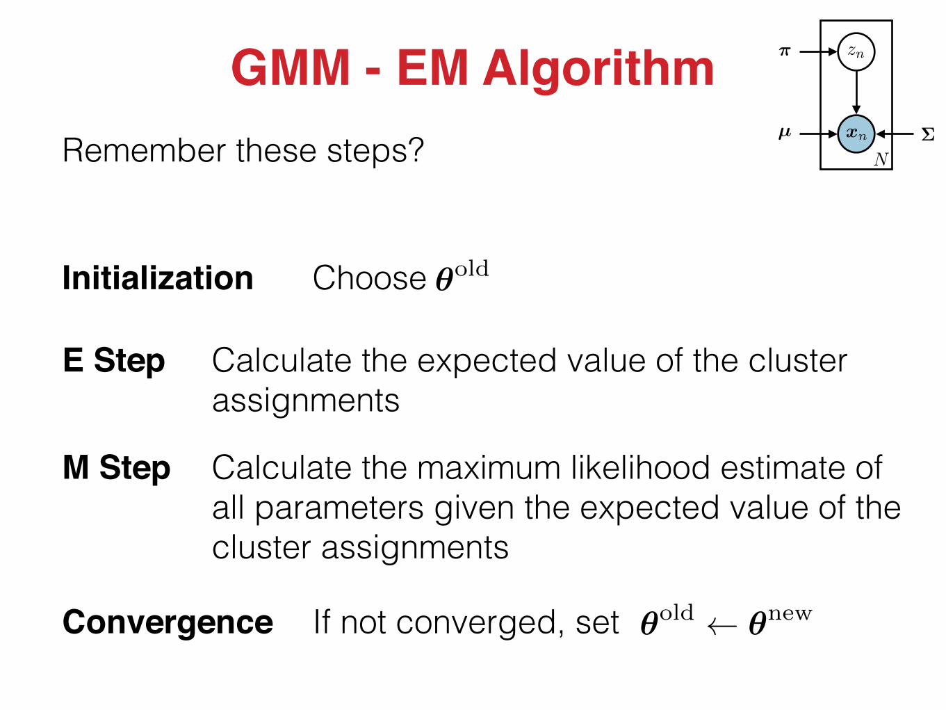
Remember these steps?
GMM - EM Algorithmxnµ
⇡
⌃
zn
N
✓oldInitialization Choose
E Step
M Step Calculate the maximum likelihood estimate of all parameters given the expected value of the cluster assignments
Convergence If not converged, set ✓old ✓new

Calculate
Remember these steps?
GMM - EM Algorithmxnµ
⇡
⌃
zn
N
✓oldInitialization Choose
p(z | x,✓old)E Step
M Step Solve✓
new= argmax
✓
Ez|x,✓old
{log p(x, z | ✓)}
Convergence If not converged, set ✓old ✓new

xnµ
⇡
⌃
zn
N
p(znk = 1 | xn,✓) =p(znk = 1)p(xn | znk = 1)
PKk0=1 p(z
nk0 = 1)p(xn | znk0 = 1)
=⇡kN (xn | µk,⌃k)PK
k0=1 ⇡k0N (xn | µk0 ,⌃k0)
GMM - E StepCalculate p(z | x,✓old)
We can think of that quantity as the responsibility that the corresponding mixture component takes for “explaining” observation
x
n
r(znk )
�

xnµ
⇡
⌃
zn
N
GMM - M StepSolve
✓
new= argmax
✓
Ez|x,✓old
{log p(x, z | ✓)}
p(zn) =KY
k=1
⇡znk
kp(xn | zn) =KY
k=1
N (xn | µk,⌃k)znk⇢
p(x, z | ✓) =NY
n=1
KY
k=1
[⇡kN (x
n | µk,⌃k)]znk
log p(x, z | ✓) =NX
n=1
KX
k=1
znk logN (x
n | µk,⌃k) + znk log ⇡k
Ez|x,✓old{log p(x, z | ✓)} =
NX
n=1
KX
k=1
r(znk ) logN (x
n | µk,⌃k) + r(znk ) log ⇡k

xnµ
⇡
⌃
zn
N
GMM - M StepSolve
✓
new= argmax
✓
Ez|x,✓old
{log p(x, z | ✓)}
✓
new= argmax
✓
NX
n=1
KX
k=1
r(znk ) logN (x
n | µk,⌃k) + r(znk ) log ⇡k
�
f(✓) = L(✓)� �
KX
k=1
⇡k � 1
!
We also have a constraint and we will use a trick called a Lagrange multiplier to make sure it is satisfied while optimizing the likelihood. We will change our maximization objective to the following, for some
Penalty for violating the constraint
⇢L(✓)
KX
k=1
⇡k = 1

@f(✓)
@�= 1�
KX
k=1
⇡k = 0 )KX
k=1
⇡k = 1
f(✓) =NX
n=1
KX
k=1
r(znk ) logN (x
n | µk,⌃k) + r(znk ) log ⇡k � �
KX
k=1
⇡k � 1
!xnµ
⇡
⌃
zn
N
GMM - M Step
Solve for ⇡k
� =KX
k=1
NX
n=1
r(znk ) = N ⇡k =Nk
N
@f(✓)
@⇡k=
PNn=1 r(z
nk )
⇡k� � = 0 ) ⇡k =
PNn=1 r(z
nk )
�=
Nk
�
Effective number of samples for which this mixture component is
responsible for

f(✓) =NX
n=1
KX
k=1
r(znk ) logN (x
n | µk,⌃k) + r(znk ) log ⇡k � �
KX
k=1
⇡k � 1
!xnµ
⇡
⌃
zn
N
GMM - M Step
@f(✓)
@µk
=NX
n=1
r(znk )⌃�1(xn � µk) = 0 ) µk =
1
Nk
NX
n=1
r(znk )xn
@f(✓)
@⌃k=
1
2
NX
n=1
r(znk )⌃�1k
⇥(xn � µk)(x
n � µk)>⌃�1
k � 1⇤= 0 )
⌃k =1
Nk
NX
n=1
r(znk )(xn � µk)(x
n � µk)>
Note that if the clusters were observed, then all the responsibilities would be indicator functions
Solve for and µk ⌃k

GMM - EM Algorithmxnµ
⇡
⌃
zn
N
r(znk ) =⇡kN (xn | µk,⌃k)PK
k0=1 ⇡k0N (xn | µk0 ,⌃k0)ComputeE Step
Nk =NX
n=1
r(znk )
⇡k =Nk
Nµk =
1
Nk
NX
n=1
r(znk )xn
⌃k =1
Nk
NX
n=1
r(znk )(xn � µk)(x
n � µk)>
M Step Compute
Convergence Iterate until the log-likelihood converges
Choose initial values for Initialization ✓ = {⇡,µ,⌃}

GMM Example - Data Set

GMM Example - Data Set

GMM Example - Iteration 1

GMM Example - Iteration 2

GMM Example - Iteration 5

GMM Example - Converged

GMM Example - Summary
Pretty good! However, initialization matters…remember that EM only
guarantees a local maximum

GMM Example - Bad Initialization
However, there are ways to deal with that… e.g., k-means++

GMM Example - Number of Clusters
However, there are ways to deal with that too…
e.g., nonparametric models

For GMMs we had the following form
probability of the corresponding
cluster
p(xn, zn) = p(xn | zn)p(zn)
p(znk = 1) = ⇡k ) p(zn) =KY
k=1
⇡znk
k
because only one cluster can be
“active” at any time
KX
k=1
⇡k = 1
A Small Variation to GMM

What if we change it to this?
A Small Variation to GMM
p(xn, zn) = p(xn | zn)p(zn)
p(znk = 1) = 1{n=argminn0 kxn0�µkk2} ) p(zn) =KY
k=1
⇡znk
k
The expectation is now simply equal to this indicator and the E step of EM simply sets the cluster of an observation to the cluster with mean closest to that
observation

If we also fix the covariance matrix to be the identity matrix, the we get the following algorithm
Initialize the cluster means arbitrarilyInitialization
Compute Nk =NX
n=1
r(znk )µk =1
Nk
NX
n=1
r(znk )xnM Step
Convergence Iterate until the means converge
ComputeE Step r(znk ) = 1{n=argminn0 kxn0�µkk2}
A Small Variation to GMM

If we also fix the covariance matrix to be the identity matrix, the we get the following algorithm
k-Means Algorithm
Initialize the cluster means arbitrarilyInitialization
Compute Nk =NX
n=1
r(znk )µk =1
Nk
NX
n=1
r(znk )xnM Step
Convergence Iterate until the means converge
ComputeE Step r(znk ) = 1{n=argminn0 kxn0�µkk2}
This is just another way to view the famous k-means clustering algorithm from an EM perspective

EM Algorithm Recap
Guaranteed to find a local maximum
Given a joint distribution over observed variables and latent variables , parameterized by , we want to maximize with respect to
p(x, z | ✓) x
z ✓ p(x | ✓)✓
Choose ✓oldInitialization
p(z | x,✓old)E Step Calculate
M Step Solve✓
new= argmax
✓
Ez|x,✓old
{log p(x, z | ✓)}
Convergence If not converged, set ✓old ✓new

EM Algorithm Recap
Another approximate inference method for probabilistic models is variational inference and it is actually a generalization of EM
EM can be used in any probabilistic model and not just Bayesian networks — undirected graphical models are an example

Bayesian Network Structure Learning
Learning structure is not that easy
• In general requires lots of data (can overfit easily) • Huge search space — we use priors to constrain it
But there exist some algorithms for certain special cases (e.g., Chow-Liu for tree structures)

Chow-Liu AlgorithmFinds the “best” tree-structured Bayesian networkWe have the following random variables
X1 X2 XN…Let the true distribution be
p(X) = p(X1, . . . , XN )
Let our tree-structured approximate distribution beq(X) = q(X1, . . . , XN )
Chow-Liu finds the that minimizes KL divergence with
q(X)p(X)
KL(p(X) || q(X)) ,X
x
p(X = x) log
p(X = x)
q(X = x)

Chow-Liu AlgorithmNotice that
only term that depends on edges
KL(p(X) || q(X)) =
X
x
p(x) logp(x)
q(x)
=
X
x
p(x) log p(x)�X
x
p(x) log q(x)
= �H(X)�NX
i=1
X
x
p(x) log p(xi | Pa(xi))
= �H(X)�NX
i=1
X
x
p(x) log p(xi) +
NX
i=1
X
x
p(x) logp(xi)
p(xi | Pa(xi))
= �H(X) +
NX
i=1
H(Xi)�NX
i=1
MI(Xi,Pa(Xi))
| {z }
q(x) =NY
i=1
p(xi | Pa(xi))
Tree Structure

Chow-Liu AlgorithmAll we need to do is find the tree that maximizes the sum of the mutual information over each edge
NX
i=1
MI(Xi,Pa(Xi)) =
NX
i=1
X
x
p(xi,Pa(xi)) logp(xi,Pa(xi))
p(xi)p(Pa(xi))
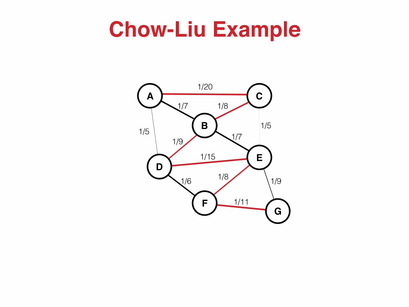
Algorithm1. For each pair of variables use observations to estimate
, , and , and calculate the mutual information 2. Compute the maximum spanning tree over all variables using
the mutual information of each pair as the corresponding edge weight
3. Add arrows to the edges to form a directed acyclic graph (DAG) 4. Learn the conditional probability tables (CPT) for this graph
A,B p(A)p(B) p(A,B)

Chow-Liu Example
A
B
C
DE
FG
1/20
1/81/7
1/51/5
1/9 1/7
1/15
1/6 1/8
1/11
1/9

Chow-Liu Example
A
B
C
DE
FG
1/20
1/81/7
1/51/5
1/9 1/7
1/15
1/6 1/8
1/11
1/9

Chow-Liu Example
A
B
C
DE
FG
1/20
1/81/7
1/51/5
1/9 1/7
1/15
1/6 1/8
1/11
1/9

Chow-Liu Example
A
B
C
DE
FG
1/20
1/81/7
1/51/5
1/9 1/7
1/15
1/6 1/8
1/11
1/9

Chow-Liu Example
A
B
C
DE
FG
1/20
1/81/7
1/51/5
1/9 1/7
1/15
1/6 1/8
1/11
1/9

Chow-Liu Example
A
B
C
DE
FG
1/20
1/81/7
1/51/5
1/9 1/7
1/15
1/6 1/8
1/11
1/9

Chow-Liu Example
A
B
C
DE
FG
1/20
1/81/7
1/51/5
1/9 1/7
1/15
1/6 1/8
1/11
1/9

Chow-Liu Example
A
B
C
DE
FG
1/20
1/81/7
1/51/5
1/9 1/7
1/15
1/6 1/8
1/11
1/9

Chow-Liu Example
A
B
C
DE
FG
1/20
1/81/7
1/51/5
1/9 1/7
1/15
1/6 1/8
1/11
1/9

Chow-Liu Example
A
B
C
DE
FG
1/20
1/81/7
1/51/5
1/9 1/7
1/15
1/6 1/8
1/11
1/9
Chow-Liu Example
A
B
C
DE
FG
1/20
1/81/7
1/51/5
1/9 1/7
1/15
1/6 1/8
1/11
1/9

Chow-Liu Example
A
B
C
DE
FG

Chow-Liu Example
A
B
C
DE
FG

…
Y
X1 X2 XN
Naive Bayes
Tree AugmentedNaive BayesUsing Chow-Liu to learn the tree structure
…
Y
X1 X2 XN

Bayesian Networks RecapBayesian Networks• Model conditional independence assumptions• Model the joint probability distribution of variables • Combine prior knowledge over:
- Dependencies - Parameter values
Inference• NP-hard in general • Has closed-form solution for some graphs • Approximate methods exist (e.g., Monte Carlo methods)Learning• Easy for fully observed data with known graph structure • Using EM for partially observed data with known graph structure • Structure learning is generally hard (possible with Chow-Liu for tree-
structured networks) • Structure learning very hard with partially observed data

Questions?