1

Heteroskedasticity and Homoskedasticity,

and Homoskedasticity-Only Standard Errors

(Section 5.4)

What…?

Consequences of homoskedasticity

Implication for computing standard errors

What do these two terms mean?

If var(u|X=x) is constant – that is, if the variance of the

conditional distribution of u given X does not depend on X –

then u is said to be homoskedastic. Otherwise, u is

heteroskedastic.

2

Homoskedasticity in a picture:

E(u|X=x) = 0 (u satisfies Least Squares Assumption #1)

The variance of u does not depend on x

3

Heteroskedasticity in a picture:

E(u|X=x) = 0 (u satisfies Least Squares Assumption #1)

The variance of u does depends on x: u is heteroskedastic.

4

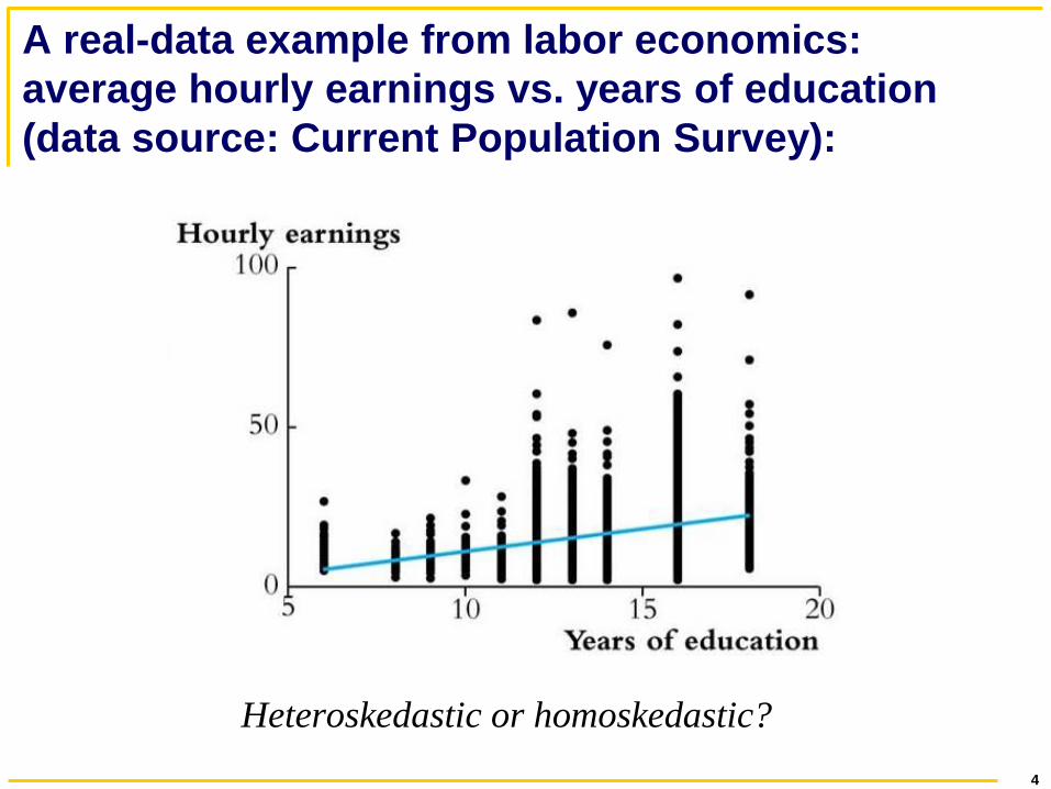
A real-data example from labor economics:

average hourly earnings vs. years of education

(data source: Current Population Survey):

Heteroskedastic or homoskedastic?

5

The class size data:

Heteroskedastic or homoskedastic?

6

So far we have (without saying so) assumed

that u might be heteroskedastic.

Recall the three least squares assumptions:

1. E(u|X = x) = 0

2. (Xi,Yi), i =1,…,n, are i.i.d.

3. Large outliers are rare

Heteroskedasticity and homoskedasticity concern var(u|X=x).

Because we have not explicitly assumed homoskedastic errors,

we have implicitly allowed for heteroskedasticity.

7

We now have two formulas for

standard errors for 1̂

Homoskedasticity-only standard errors – these are valid only

if the errors are homoskedastic.

The usual standard errors – to differentiate the two, it is

conventional to call these heteroskedasticity – robust

standard errors, because they are valid whether or not the

errors are heteroskedastic.

The main advantage of the homoskedasticity-only standard

errors is that the formula is simpler. But the disadvantage is

that the formula is only correct in general if the errors are

homoskedastic.

8

Practical implications… The homoskedasticity-only formula for the standard error of

1̂ and the “heteroskedasticity-robust” formula differ – so in

general, you get different standard errors using the different

formulas.

Homoskedasticity-only standard errors are the default setting

in regression software – sometimes the only setting (e.g.

Excel). To get the general “heteroskedasticity-robust”

standard errors you must override the default.

If you don’t override the default and there is in fact

heteroskedasticity, your standard errors (and wrong t-

statistics and confidence intervals) will be wrong – typically,

homoskedasticity-only SEs are too small.

9

Heteroskedasticity-robust standard

errors in STATA regress testscr str, robust

Regression with robust standard errors Number of obs = 420

F( 1, 418) = 19.26

Prob > F = 0.0000

R-squared = 0.0512

Root MSE = 18.581

-------------------------------------------------------------------------

| Robust

testscr | Coef. Std. Err. t P>|t| [95% Conf. Interval]

--------+----------------------------------------------------------------

str | -2.279808 .5194892 -4.39 0.000 -3.300945 -1.258671

_cons | 698.933 10.36436 67.44 0.000 678.5602 719.3057

-------------------------------------------------------------------------

If you use the “, robust” option, STATA computes

heteroskedasticity-robust standard errors

Otherwise, STATA computes homoskedasticity-only

standard errors

10

The bottom line:

If the errors are either homoskedastic or heteroskedastic and

you use heteroskedastic-robust standard errors, you are OK

If the errors are heteroskedastic and you use the

homoskedasticity-only formula for standard errors, your

standard errors will be wrong (the homoskedasticity-only

estimator of the variance of 1̂ is inconsistent if there is

heteroskedasticity).

The two formulas coincide (when n is large) in the special

case of homoskedasticity

So, you should always use heteroskedasticity-robust standard

errors.

11

Some Additional Theoretical

Foundations of OLS (Section 5.5)

We have already learned a very great deal about OLS: OLS is

unbiased and consistent; we have a formula for

heteroskedasticity-robust standard errors; and we can construct

confidence intervals and test statistics.

Also, a very good reason to use OLS is that everyone else

does – so by using it, others will understand what you are doing.

In effect, OLS is the language of regression analysis, and if you

use a different estimator, you will be speaking a different

language.

12

The Extended Least Squares

Assumptions

These consist of the three LS assumptions, plus two more:

1. E(u|X = x) = 0.

2. (Xi,Yi), i =1,…,n, are i.i.d.

3. Large outliers are rare (E(Y4) < , E(X

4) < ).

4. u is homoskedastic

5. u is distributed N(0,2)

Assumptions 4 and 5 are more restrictive – so they apply to

fewer cases in practice. However, if you make these

assumptions, then certain mathematical calculations simplify

and you can prove strong results – results that hold if these

additional assumptions are true.

We start with a discussion of the efficiency of OLS

13

Efficiency of OLS, part I: The

Gauss-Markov Theorem

Under extended LS assumptions 1-4 (the basic three, plus

homoskedasticity), 1̂ has the smallest variance among all linear

estimators (estimators that are linear functions of Y1,…, Yn).

This is the Gauss-Markov theorem.

Comments

The GM theorem is proven in SW Appendix 5.2

14

Efficiency of OLS, part II:

Under all five extended LS assumptions – including normally

distributed errors – 1̂ has the smallest variance of all

consistent estimators (linear or nonlinear functions of

Y1,…,Yn), as n .

This is a pretty amazing result – it says that, if (in addition to

LSA 1-3) the errors are homoskedastic and normally

distributed, then OLS is a better choice than any other

consistent estimator. And because an estimator that isn’t

consistent is a poor choice, this says that OLS really is the best

you can do – if all five extended LS assumptions hold. (The

proof of this result is beyond the scope of this course and isn’t

in SW – it is typically done in graduate courses.)

15

Some not-so-good thing about OLS

The foregoing results are impressive, but these results – and the

OLS estimator – have important limitations.

1. The GM theorem really isn’t that compelling:

The condition of homoskedasticity often doesn’t hold

(homoskedasticity is special)

The result is only for linear estimators – only a small

subset of estimators (more on this in a moment)

2. The strongest optimality result (“part II” above) requires

homoskedastic normal errors – not plausible in applications

(think about the hourly earnings data!)

16

Limitations of OLS, ctd.

3. OLS is more sensitive to outliers than some other estimators.

In the case of estimating the population mean, if there are big

outliers, then the median is preferred to the mean because the

median is less sensitive to outliers – it has a smaller variance

than OLS when there are outliers. Similarly, in regression,

OLS can be sensitive to outliers, and if there are big outliers

other estimators can be more efficient (have a smaller

variance). One such estimator is the least absolute deviations

(LAD) estimator:

0 1, 0 1

1

min ( )n

b b i i

i

Y b b X

In virtually all applied regression analysis, OLS is used – and

that is what we will do in this course too.

17

Summary and Assessment

(Section 5.7) The initial policy question:

Suppose new teachers are hired so the student-teacher

ratio falls by one student per class. What is the effect

of this policy intervention (“treatment”) on test scores?

Does our regression analysis answer this convincingly?

Not really – districts with low STR tend to be ones with

lots of other resources and higher income families,

which provide kids with more learning opportunities

outside school…this suggests that corr(ui, STRi) > 0, so

E(ui|Xi) 0.

So, we have omitted some factors, or variables, from our

analysis, and this has biased our results.