and government debt dynamics interest-rate-growth ... · 1. the importance of the...

From:OECD Journal: Economic Studies

Access the journal at:http://dx.doi.org/10.1787/19952856

Interest-rate-growth differentialsand government debt dynamics

David Turner, Francesca Spinelli

Please cite this article as:

Turner, David and Francesca Spinelli (2012), “Interest-rate-growthdifferentials and government debt dynamics”, OECD Journal:Economic Studies, Vol. 2012/1.http://dx.doi.org/10.1787/eco_studies-2012-5k912k0zkhf8

http://dx.doi.org/10.1787/19952856

http://dx.doi.org/10.1787/eco_studies-2012-5k912k0zkhf8

This document and any map included herein are without prejudice to the status of orsovereignty over any territory, to the delimitation of international frontiers and boundaries and tothe name of any territory, city or area.

OECD Journal: Economic Studies

Volume 2012

© OECD 2013

103

Interest-rate-growth differentialsand government debt dynamics

by

David Turner and Francesca Spinelli*

The differential between the interest rate paid to service government debt and thegrowth rate of the economy is a key concept in assessing fiscal sustainability.Among OECD economies, this differential was unusually low for much of the lastdecade compared with the 1980s and the first half of the 1990s. This articleinvestigates the reasons behind this profile using panel estimation on selectedOECD economies as means of providing some guidance as to its future development.The results suggest that the fall is partly explained by lower inflation volatilityassociated with the adoption of monetary policy regimes credibly targeting lowinflation, which might be expected to continue. However, the low differential is alsopartly explained by factors which are likely to be reversed in the future, includingvery low policy rates, the “global savings glut” and the effect which the EuropeanMonetary Union had in reducing long-term interest differentials in the pre-crisisperiod. The differential is also likely to rise in the future because the number ofcountries which have debt-to-GDP ratios above a threshold at which there appearsto be an effect on sovereign risk premia has risen sharply. Moreover, debt isprojected to increasingly rise above this threshold in most of these countries.

JEL classification: E43, E62, H63, H68

Keywords: fiscal sustainability, government debt, interest rates, interest-rate-growth differential.

* David Turner ([email protected]) and Francesca Spinelli ([email protected]) are membersof the Macroeconomic Analysis Division of the OECD Economics Department. They would like tothank participants of the UN DESA Expert Group meeting on the World Economy (LINK Project) heldon 24-26 October 2011 for comments on an early presentation of this work. In addition, they wouldlike to thank Jean-Luc Schneider, Jørgen Elmeskov, Lukasz Rawdanowicz, Yvan Guillemette,Stéphanie Guichard and Mauro Pisu for helpful comments on the paper as well as Diane Scott forhelp in the final document preparation. The views expressed in this article are those of the authorsand do not necessarily represent those of the OECD or its member countries.

INTEREST-RATE-GROWTH DIFFERENTIALS AND GOVERNMENT DEBT DYNAMICS

OECD JOURNAL: ECONOMIC STUDIES – VOLUME 2012 © OECD 2013104

The financial crisis has led to severe fiscal imbalances in many OECD countries. Difficult

decisions need to be addressed concerning the speed with which to close wide fiscal

deficits given the underlying weakness of activity as well as concerns about long-run fiscal

sustainability given ballooning government indebtedness. A key issue in assessing

long-run fiscal sustainability is the future trend of the differential between the interest rate

paid to service government debt and the growth rate of the economy. For highly indebted

countries, a change in this differential of a couple of percentage points, if sustained,

could mean the difference between an explosive and a declining path for the debt-to-GDP

ratio. Indeed, the focus among policy-makers, the media and financial markets on both the

level of long-term interest rates and the prospects for growth during the ongoing euro area

crisis underlines the importance of this differential as a measure of fiscal sustainability.

In this context, it matters a lot whether OECD countries are likely to face the

low interest-rate-growth differential environment which typically prevailed over much

of the pre-crisis 2000s or the much higher and less favourable differential which was

typical of the 1980s and the first half of the 1990s.1 Among a group of selected OECD

countries considered in this article the median interest-rate-growth differential fell from

almost 2½ percentage points to about zero between these periods, with a much greater fall

for those countries which initially had a larger differential. This article attempts to

evaluate the relative importance of various explanations for the fall in the differential as a

guide to understanding possible future trends, particularly given that there is little in the

way of existing published analytical work which looks at this issue in a multi-country

framework.2

The main findings of the article are as follows:

● The decline in uncertainty surrounding inflation, associated with the decline in the level

and more particularly the volatility of inflation, has almost certainly contributed to a fall

in the interest-rate-growth differential. The empirical work reported in this article

suggests that it might have contributed between ¾ and 1 percentage point for the typical

OECD country, and by more for those countries where inflation volatility has declined

by more. This change is probably the consequence of a general move in the use of

monetary policy towards a more credible targeting of inflation. To the extent that

inflation expectations remain anchored in the future these gains might be expected to

persist. This also suggests some caution in policy-makers attempting to reduce

government indebtedness by deliberately engineering a period of high inflation. A period

of unexpectedly high inflation will, ceteris paribus, tend to reduce the debt ratio,

particularly the longer the maturity structure of debt (see Box 1.8 in OECD Economic

Outlook No. 80). However, this effect could be easily offset if higher inflation led to greater

uncertainty about future inflation and so a permanently higher interest-rate-growth

differential.


OECD JOURNAL: ECONOMIC STUDIES – VOLUME 2012 © OECD 2013 105

● On the other hand, other factors behind the low differential over the last decade are

unlikely to persist over the longer term and their reversal is likely to result in an increase

in the differential:

❖ Policy rates and short-term interest rates were unusually low for an unusually long

time over the last decade, partially in response to fears about the severity of the

downturn and the risks of deflation following the sharp fall in equity prices at the end

of the 1990s. This, by creating expectations of future low interest rates, almost

certainly dragged down long-term interest rates. In the wake of the financial crisis,

policy rates in many countries have been further cut to extremely low levels. Although

this situation may continue for a few (or even many) years, over the longer run as

policy rates normalise this is likely to push up the interest-rate-growth differential.

Estimates in this article suggest that for a typical OECD country this will imply a rise

in the interest-rate-growth differential by around 1 to 1¼ percentage points.

❖ This article provides some tentative empirical support for the effect of a “Global Savings

Glut” originating from Asian emerging markets and oil exporters with an estimated

effect of reducing the interest-rate-growth differential during the 2000s by around 1¼ to

1½ percentage points. Such a global savings-investment imbalance is unlikely to persist

indefinitely. Indeed, there are arguments to suggest that future trends in global savings

and investment are more likely to put upward pressure on global interest rates and

hence raise the interest-rate-growth differential (Dobbs et al., 2010).

❖ Other research suggests that quantitative easing measures undertaken since the

financial crisis may have reduced long-term interest rates by up to 100 basis points,

implying that as the effect of such measures fades there will be a corresponding

increase in long-term interest rates.

● One factor which is likely to exert a much larger positive influence on the interest-rate-

growth differential over the future is higher fiscal sovereign risk premia associated with

increased government indebtedness, which for many countries has increased

substantially in the wake of the crisis. Some evidence is found in support of a threshold

effect, whereby each percentage point increase in the gross government debt-to-GDP

ratio above 75% of GDP leads to an increase in the differential of 4 basis points. According

to recent OECD projections (OECD, 2011), there are likely to be 15 OECD countries with

debt ratios exceeding this threshold compared with just six countries immediately prior

to the crisis.

● Relative to the pre-crisis period, the change in the interest-rate-growth differential may

be particularly large for some euro area countries, as it is clear that over the pre-crisis

period the introduction of European Monetary Union led to a marked convergence of

long-term interest rates among member countries so masking the effect of individual

country characteristics such as indebtedness. Moreover, since the crisis there is evidence

to suggest that, ceteris paribus, interest rates in euro countries are more sensitive to

indebtedness than other OECD countries, a prediction consistent with the inability of

members of a currency union to freely issue their own currency in response to increased

government indebtedness. However the current euro area sovereign debt crisis is

resolved, it seems likely that fundamentals will play a more important role in

determining long-term interest rates of individual countries within EMU in the future.



The remainder of the article is organised as follows: Section 1 explains the importance

of the interest-rate-growth differential in debt dynamics with a specific illustration with

respect to the US fiscal position; Section 2 considers various measurement issues and

examines past trends in the differential for OECD countries; Section 3 describes some of

the possible explanations for past trends in the differential, namely changes in inflation

volatility, policy rates, the “global savings glut”, European Monetary Union and government

indebtedness; finally, Section 4 attempts to discriminate between these explanations using

panel estimations on a large number of OECD countries.

1. The importance of the interest-rate-growth differential in debt dynamicsThe interest-rate-growth differential is essential to understanding long-run fiscal

sustainability; higher interest rates imply higher interest payments to service government

debt so adversely influencing debt dynamics, whereas higher nominal GDP growth will

tend to lower the debt-to-GDP ratio by increasing the denominator. More formally, the

importance of the interest-rate-growth differential can be seen from the government

budget identity,3 whereby the change in the net government debt-to-GDP ratio (d) is

explained by the primary deficit ratio (-pb) plus net interest rates payments on the previous

period’s debt, where it is the effective interest rate paid on net government debt, so that

approximately:

dt = – pbt + (it – gt) dt-1, (1)

where gt is the nominal GDP growth rate. Thus, for a given primary balance and initial net

debt ratio, the rate of increase in the debt-to-GDP ratio is positively related to the interest-

rate-growth differential.

In order to illustrate the importance of the interest-rate-growth differential in long-

term fiscal projections, the sensitivity of recently published OECD fiscal projections to

alternative assumptions regarding this differential are considered. The long-term

projections published in June 2011 (OECD, 2011) are based on the stylised assumption that

beyond 2012 gradual fiscal consolidation, equal to an improvement in the underlying

primary balance of ½ percentage point of GDP each year, is undertaken until the debt-

to-GDP ratio is stabilised. The United States is one of only two OECD countries for which

the stylised gradual fiscal consolidation would be insufficient to stabilise the government

debt-to-GDP ratio by 2026, with gross general government debt reaching nearly 150% of

GDP, although the rate of increase in the debt ratio is clearly diminishing (Figure 1). The

importance of the interest-rate-growth differential in debt dynamics, particularly for a

highly-indebted country, is illustrated by the substantial difference in two variant

simulations in which the differential is alternatively increased and then decreased

by 2 percentage points relative to this baseline, assuming that the primary balance

remains the same as in the baseline.4

The calculations underlying this illustrative example ignore the likely interactions and

feedback effects from the variables included in the government budget identity (1). For

example, if the government boosts the primary surplus in response to a deterioration in

the interest-rate-growth differential then a trend increase in the debt ratio could be

avoided. On the other hand, other feedback effects may exacerbate the effect of the

differential on debt projections:

● The shock to the differential is applied ex post, whereas if applied ex ante there might be

reasons to expect further changes to the differential which re-enforce the effect of the



original shock; for example, if debt begins to rise as a consequence of a higher

differential then fiscal risk premium on debt might be expected to rise; also at higher

levels of debt there is some empirical evidence to suggest that there may be some

adverse effect on real growth rates (Reinhart and Rogoff, 2010).

● These stylised fiscal projections are based on the assumption that primary public

expenditure remains a stable share of GDP. However, if the differential falls as a result of

faster growth it is likely that some components of public expenditure, such as

infrastructure expenditure, would rise less than proportionately, which in turn would

imply a more rapid reduction in debt.

2. Measurement issuesIn analysing historical trends, the interest-rate-growth differential is here defined

differently from how it appears in the budget identity described in equation (1) above. This

is both to improve cross-country comparability, which is important when undertaking

panel regressions, and to provide a better trend measure which abstracts from volatility,

particularly that associated with the cycle, thus:

● Nominal potential GDP growth is used in place of actual GDP growth in order to reduce

the volatility associated with the business cycle given that the focus here is on long-term

fiscal sustainability. The estimates of potential output which are used are those

described in OECD (2011) and are intended to measure the trend level of output which

can be sustained without inflationary pressure.

● The interest rate that is used in the analysis here is that on 10-year government bonds

which differs from the concept of the implicit interest rate on net government debt used

in the budget identity (1) in a number of ways:

❖ The interest rate in the budget identity is the implicit net interest rate paid on net debt

and so takes into account the interest receipts earned on government asset holdings.

Figure 1. Sensitivity of debt projections to the interest-rate-growth differentialGross government debt of Unites States as percentage of GDP

Source: OECD Economic Outlook, June 2011, and OECD calculations.

0

40

80

120

160

200

2000

2001

2002

2003

2004

2005

2006

2007

2008

2009

2010

2011

2012

2013

2014

2015

2016

2017

2018

2019

2020

2021

2022

2023

2024

2025

2026

Baseline, OECD Economic Outlook June 2011

Baseline, +/- 2% pts on the interest-rate-growth differential



Nevertheless, the empirical analysis here focuses on the rates on 10-year government

bonds because there is great heterogeneity in the size and composition of government

assets holdings across countries.

❖ The interest rate in the budget identity is the average implicit interest rate paid on all

debt which will differ from the interest rate on new issues of government debt. Thus,

for example, after a prolonged period when long-term interest rates have been

unusually low for a long period (perhaps, for example, because short-term policy rates

have been low for cyclical reasons) but have recently begun to rise, then the average

interest rate paid on gross government debt will be lower than the rate on new bond

issues. However, the latter will provide a more timely indicator of the future trends in

the cost of government financing.

❖ The interest rate which is used in the analysis is that on 10-year government bonds

which will differ from even the rate of new bond issues if these are issued at different

maturities. An argument for using the former in the analysis is that it is both simpler

to implement and will abstract from differences across countries regarding the

maturity structure of new bond issues which may well be temporary.

❖ Finally, using a measure of the implicit rate on net government debt in regression

analysis is ruled out for many countries because when net government debt (the

denominator in any calculation of the implicit rate) becomes very low the implicit rate

can easily jump to absurd levels.

Based on the definitions described above (see Annex A1 for further details of the data),

the interest-rate-growth differential for a group of OECD countries, for which consistent

time series of data is available, shows a marked fall during the 1970s (Figure 2) as the

inflation rate rose very substantially from levels experienced during the 1960s (Figure 3). As

inflation surprises subsided, the level of the interest-rate-growth differential was much

higher and for nearly all countries positive during the 1980s and the first half of the 1990s.

Figure 2. The interest-rate-growth differential for selected OECD countriesPercentage points

Source: OECD Economic Outlook, June 2011, and OECD calculations, country coverage varies over the sample period, seenotes to Table 1 and Annex A1 for further details.

-16

-12

-8

-4

0

4

8

1970

1972

1974

1976

1978

1980

1982

1984

1986

1988

1990

1992

1994

1996

1998

2000

2002

2004

2006

2008

2010

Median

Lower / Upper quartiles



The differential then exhibits a marked fall from its median level in the 1980s and first half

of the 1990s of typically about 2½ percentage points to close to zero during the pre-crisis

2000s (Figure 2 and Table 1). Moreover, there are many countries (e.g. Australia, Canada,

Denmark, Spain, Ireland and Norway) where the interest rate-growth-differential fell by

4 percentage points or more between these two periods.

Figure 3. The level and volatility of OECD inflationChange in the OECD-wide GDP deflator, percentage points

Source: OECD Economic Outlook, June 2011, and OECD calculations. For country coverage see notes to Table 1 and seeAnnex A1 for further details.

Table 1. The interest-rate-growth differential for selected OECD countries

1970-79 1980-95 1996-99 2000-08 2010

G7 countries

Upper quartile –2.46 3.22 2.41 1.50 1.60

Median -3.82 2.32 1.61 0.41 0.95

Lower quartile –5.80 1.28 0.92 –0.19 0.12

Number of countries 6 7 7 7 7

Selected OECD countries1

Upper quartile –1.80 3.80 2.41 0.68 1.76

Median –3.36 2.41 1.42 –0.11 0.53

Lower quartile –5.17 0.79 0.33 –1.40 –1.00


Selected EMU countries2

Upper quartile –2.29 3.70 2.40 0.74 3.80

Median –3.66 2.64 0.98 –0.11 1.34

Lower quartile –4.83 1.06 –0.13 –1.50 0.85


1. Australia, Austria, Belgium, Canada, Denmark, Finland, France, Germany, Greece, Iceland, Ireland, Italy, Japan, Korea,the Netherlands, New Zealand, Norway, Portugal, Spain, Sweden, Switzerland, United Kingdom, United States.

2. Austria, Belgium, Finland, France, Germany, Greece, Ireland, Italy, Netherlands, Portugal, Spain.Source: OECD Economic Outlook, June 2011, and OECD calculations. See Annex A1 for further details.

0

4

8

12

1619

65

1967

1969

1971

1973

1975

1977

1979

1981

1983

1985

1987

1989

1991

1993

1995

1997

1999

2001

2003

2005

2007

2009

OECD Inflation (GDP deflator) OECD Inflation volatility (5 year standard deviation)



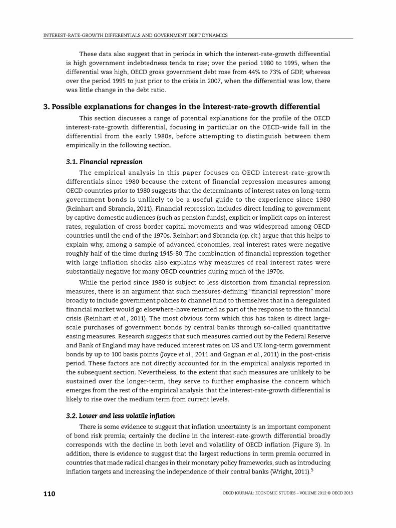
These data also suggest that in periods in which the interest-rate-growth differential

is high government indebtedness tends to rise; over the period 1980 to 1995, when the

differential was high, OECD gross government debt rose from 44% to 73% of GDP, whereas

over the period 1995 to just prior to the crisis in 2007, when the differential was low, there

was little change in the debt ratio.

3. Possible explanations for changes in the interest-rate-growth differentialThis section discusses a range of potential explanations for the profile of the OECD

interest-rate-growth differential, focusing in particular on the OECD-wide fall in the

differential from the early 1980s, before attempting to distinguish between them

empirically in the following section.

3.1. Financial repression

The empirical analysis in this paper focuses on OECD interest-rate-growth

differentials since 1980 because the extent of financial repression measures among

OECD countries prior to 1980 suggests that the determinants of interest rates on long-term

government bonds is unlikely to be a useful guide to the experience since 1980

(Reinhart and Sbrancia, 2011). Financial repression includes direct lending to government

by captive domestic audiences (such as pension funds), explicit or implicit caps on interest

rates, regulation of cross border capital movements and was widespread among OECD

countries until the end of the 1970s. Reinhart and Sbrancia (op. cit.) argue that this helps to

explain why, among a sample of advanced economies, real interest rates were negative

roughly half of the time during 1945-80. The combination of financial repression together

with large inflation shocks also explains why measures of real interest rates were

substantially negative for many OECD countries during much of the 1970s.

While the period since 1980 is subject to less distortion from financial repression

measures, there is an argument that such measures-defining “financial repression” more

broadly to include government policies to channel fund to themselves that in a deregulated

financial market would go elsewhere-have returned as part of the response to the financial

crisis (Reinhart et al., 2011). The most obvious form which this has taken is direct large-

scale purchases of government bonds by central banks through so-called quantitative

easing measures. Research suggests that such measures carried out by the Federal Reserve

and Bank of England may have reduced interest rates on US and UK long-term government

bonds by up to 100 basis points (Joyce et al., 2011 and Gagnan et al., 2011) in the post-crisis

period. These factors are not directly accounted for in the empirical analysis reported in

the subsequent section. Nevertheless, to the extent that such measures are unlikely to be

sustained over the longer-term, they serve to further emphasise the concern which

emerges from the rest of the empirical analysis that the interest-rate-growth differential is

likely to rise over the medium term from current levels.

3.2. Lower and less volatile inflation

There is some evidence to suggest that inflation uncertainty is an important component

of bond risk premia; certainly the decline in the interest-rate-growth differential broadly

corresponds with the decline in both level and volatility of OECD inflation (Figure 3). In

addition, there is evidence to suggest that the largest reductions in term premia occurred in

countries that made radical changes in their monetary policy frameworks, such as introducing

inflation targets and increasing the independence of their central banks (Wright, 2011).5



3.3. The global savings glut

According to the “global savings glut” hypothesis (Bernanke, 2005 and 2007), increased

capital inflows to the United States from countries in which desired saving greatly exceeded

desired investment – particularly Asian emerging markets and non-OECD oil exporters –

were an important reason why long-term interest rates were lower than expected in the pre-

crisis 2000s. Although the argument was originally applied to the United States, in principle

it seems likely that it might also apply more generally to the advanced OECD economies.

A crude measure of the ex ante imbalance between global savings and investment is

the ex post current account surplus of the Asian emerging markets and oil exporters

expressed as percentage of world GDP (Figure 4) which is used here in the subsequent

empirical analysis. There will, of course, always be some countries running a current

account surplus so taking a subset of these and referring to it as a measure of a “global

savings glut” is admittedly crude. Nevertheless, these countries are singled out here

because they ran up large current account surpluses so rapidly – because of massive

structural reform, fiscal adjustment or swings in commodity prices – that there was no

possibility to easily absorb the additional savings in domestic investment opportunities.

3.4. A prolonged period of low policy rates

If long-term interest rates are considered as a forward convolution of expected short-

term interest rates plus term premia, it follows that large deviations of short-term rates

which are expected to persist over a period of many years will also pull long-term interest

rates away from their more fundamental levels. Monetary policy exerts a powerful

influence on short-term market interest rates. In particular, policy rates have been

unusually low for an unusually long time over much of the last decade, in response firstly

to fears about the severity of the downturn and the risks of deflation following the sharp

Figure 4. A measure of the “global savings glut”Combined current account surpluses of Asian emerging markets and oil exporters,

as a percentage of world GDP

Source: International Monetary Fund, World Economic Outlook Database, September 2011. For further details seeAnnex A1.

-0.5

0

0.5

1

1.5

1980

1981

1982

1983

1984

1985

1986

1987

1988

1989

1990

1991

1992

1993

1994

1995

1996

1997

1998

1999

2000

2001

2002

2003

2004

2005

2006

2007

2008

2009

2010



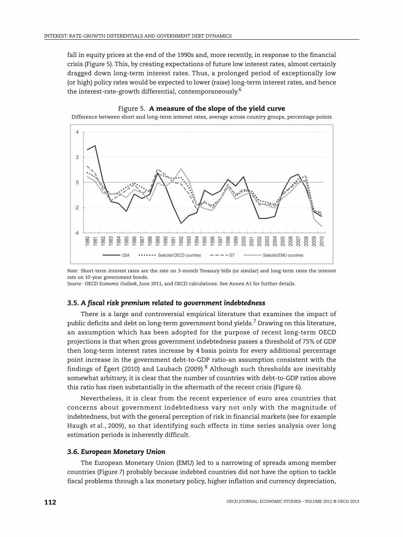
fall in equity prices at the end of the 1990s and, more recently, in response to the financial

crisis (Figure 5). This, by creating expectations of future low interest rates, almost certainly

dragged down long-term interest rates. Thus, a prolonged period of exceptionally low

(or high) policy rates would be expected to lower (raise) long-term interest rates, and hence

the interest-rate-growth differential, contemporaneously.6

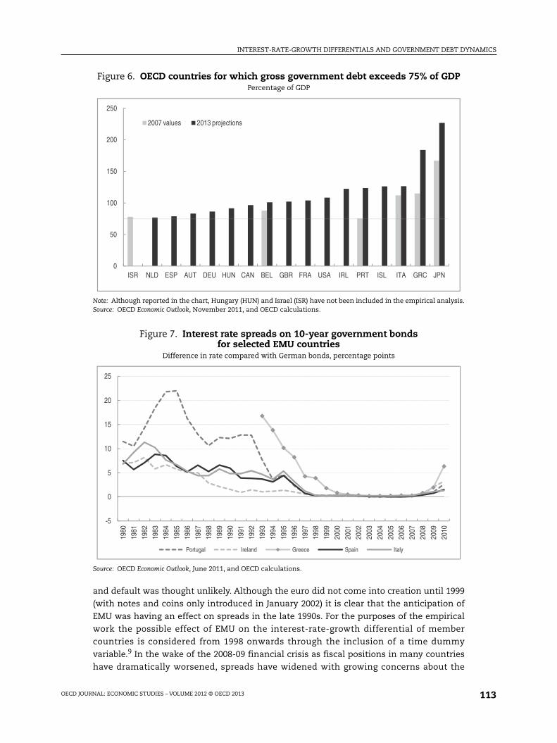
3.5. A fiscal risk premium related to government indebtedness

There is a large and controversial empirical literature that examines the impact of

public deficits and debt on long-term government bond yields.7 Drawing on this literature,

an assumption which has been adopted for the purpose of recent long-term OECD

projections is that when gross government indebtedness passes a threshold of 75% of GDP

then long-term interest rates increase by 4 basis points for every additional percentage

point increase in the government debt-to-GDP ratio-an assumption consistent with the

findings of Égert (2010) and Laubach (2009).8 Although such thresholds are inevitably

somewhat arbitrary, it is clear that the number of countries with debt-to-GDP ratios above

this ratio has risen substantially in the aftermath of the recent crisis (Figure 6).

Nevertheless, it is clear from the recent experience of euro area countries that

concerns about government indebtedness vary not only with the magnitude of

indebtedness, but with the general perception of risk in financial markets (see for example

Haugh et al., 2009), so that identifying such effects in time series analysis over long

estimation periods is inherently difficult.

3.6. European Monetary Union

The European Monetary Union (EMU) led to a narrowing of spreads among member

countries (Figure 7) probably because indebted countries did not have the option to tackle

fiscal problems through a lax monetary policy, higher inflation and currency depreciation,

Figure 5. A measure of the slope of the yield curveDifference between short and long-term interest rates, average across country groups, percentage points

Note: Short-term interest rates are the rate on 3-month Treasury bills (or similar) and long-term rates the interestrate on 10-year government bonds.Source: OECD Economic Outlook, June 2011, and OECD calculations. See Annex A1 for further details.

-4

-2

0

2

4

1980

1981

1982

1983

1984

1985

1986

1987

1988

1989

1990

1991

1992

1993

1994

1995

1996

1997

1998

1999

2000

2001

2002

2003

2004

2005

2006

2007

2008

2009

2010

USA Selected OECD countries G7 Selected EMU countries



and default was thought unlikely. Although the euro did not come into creation until 1999

(with notes and coins only introduced in January 2002) it is clear that the anticipation of

EMU was having an effect on spreads in the late 1990s. For the purposes of the empirical

work the possible effect of EMU on the interest-rate-growth differential of member

countries is considered from 1998 onwards through the inclusion of a time dummy

variable.9 In the wake of the 2008-09 financial crisis as fiscal positions in many countries

have dramatically worsened, spreads have widened with growing concerns about the

Figure 6. OECD countries for which gross government debt exceeds 75% of GDPPercentage of GDP

Note: Although reported in the chart, Hungary (HUN) and Israel (ISR) have not been included in the empirical analysis.Source: OECD Economic Outlook, November 2011, and OECD calculations.

Figure 7. Interest rate spreads on 10-year government bondsfor selected EMU countries

Difference in rate compared with German bonds, percentage points

Source: OECD Economic Outlook, June 2011, and OECD calculations.

0

50

100

150

200

250

ISR NLD ESP AUT DEU HUN CAN BEL GBR FRA USA IRL PRT ISL ITA GRC JPN

2007 values 2013 projections

-5

0

5

10

15

20

25

1980

1981

1982

1983

1984

1985

1986

1987

1988

1989

1990

1991

1992

1993

1994

1995

1996

1997

1998

1999

2000

2001

2002

2003

2004

2005

2006

2007

2008

2009

2010

Portugal Ireland Greece Spain Italy



adequacy of institutional arrangements for a lender-of-last resort to heavily indebted

member countries which come under extreme pressure from financial markets. For this

reason the EMU time dummy is not extended beyond 2008.

4. Empirical analysisIn order to assess the relative importance of the various explanations discussed in the

previous section, annual panel regressions explaining the interest-rate-growth differential

(as defined in Section 2 above) are run for selected OECD countries for which a long time

span of data is available, mostly covering the period 1980-2010.10 A potential problem in

estimation is that the inclusion of a lagged dependent variable may lead to biased

estimates (Nickell, 1981), although because the time dimension here is relatively large

(exceeding 30), the extent of the bias is likely to be small (see for example, Baltagi and

Griffin, 1997). Nevertheless, in order to correct for any possible bias, the bias corrected least

squares dummy variable estimator for dynamic unbalanced panel data models proposed

by Bruno (2005) has been applied.11

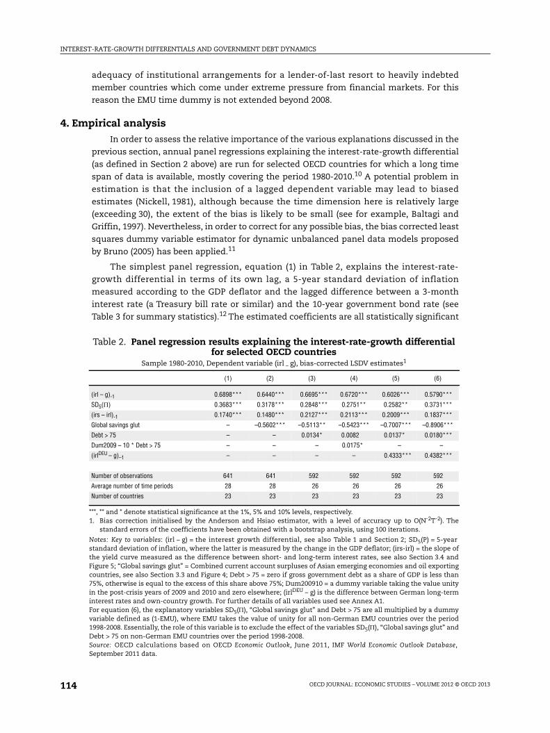
The simplest panel regression, equation (1) in Table 2, explains the interest-rate-

growth differential in terms of its own lag, a 5-year standard deviation of inflation

measured according to the GDP deflator and the lagged difference between a 3-month

interest rate (a Treasury bill rate or similar) and the 10-year government bond rate (see

Table 3 for summary statistics).12 The estimated coefficients are all statistically significant

Table 2. Panel regression results explaining the interest-rate-growth differentialfor selected OECD countries

Sample 1980-2010, Dependent variable (irl – g), bias-corrected LSDV estimates1

(1) (2) (3) (4) (5) (6)

(irl – g)-1 0.6898*** 0.6440*** 0.6695*** 0.6720*** 0.6026*** 0.5790***

SD5() 0.3683*** 0.3178*** 0.2848*** 0.2751** 0.2582** 0.3731***

(irs – irl)-1 0.1740*** 0.1480*** 0.2127*** 0.2113*** 0.2009*** 0.1837***

Global savings glut – –0.5602*** –0.5113** –0.5423*** –0.7007*** –0.8906***

Debt > 75 – – 0.0134* 0.0082 0.0137* 0.0180***

Dum2009 – 10 * Debt > 75 – – – 0.0175* – –

(irlDEU – g)–1 – – – – 0.4333*** 0.4382***

Number of observations 641 641 592 592 592 592

Average number of time periods 28 28 26 26 26 26

Number of countries 23 23 23 23 23 23

***, ** and * denote statistical significance at the 1%, 5% and 10% levels, respectively.1. Bias correction initialised by the Anderson and Hsiao estimator, with a level of accuracy up to O(N-2T-2). The

standard errors of the coefficients have been obtained with a bootstrap analysis, using 100 iterations.

Notes: Key to variables: (irl – g) = the interest growth differential, see also Table 1 and Section 2; SD5(P) = 5-yearstandard deviation of inflation, where the latter is measured by the change in the GDP deflator; (irs-irl) = the slope ofthe yield curve measured as the difference between short- and long-term interest rates, see also Section 3.4 andFigure 5; “Global savings glut” = Combined current account surpluses of Asian emerging economies and oil exportingcountries, see also Section 3.3 and Figure 4; Debt > 75 = zero if gross government debt as a share of GDP is less than75%, otherwise is equal to the excess of this share above 75%; Dum200910 = a dummy variable taking the value unityin the post-crisis years of 2009 and 2010 and zero elsewhere; (irlDEU – g) is the difference between German long-terminterest rates and own-country growth. For further details of all variables used see Annex A1.For equation (6), the explanatory variables SD5(), “Global savings glut” and Debt > 75 are all multiplied by a dummyvariable defined as (1-EMU), where EMU takes the value of unity for all non-German EMU countries over the period1998-2008. Essentially, the role of this variable is to exclude the effect of the variables SD5(), “Global savings glut” andDebt > 75 on non-German EMU countries over the period 1998-2008.Source: OECD calculations based on OECD Economic Outlook, June 2011, IMF World Economic Outlook Database,September 2011 data.



and with the expected signs. They imply that a fall in the standard deviation of inflation by

1 percentage point, which is about the typical reduction observed between the periods

1980-95 and 2000-08, will eventually lead to a decline in the interest-rate-growth

differential of just over a percentage point (Table 4).

A difference between short and long-term interest rates of 1 percentage point will

depress the interest-rate-growth differential by 0.6 percentage points. This implies that on

average the unusually low policy rates in the pre-crisis 2000s may have reduced the

interest-rate-growth differential by just under ½ percentage point relative to the period

1980-95. Given the further steepening of the yield curve since the advent of the crisis, it

Table 3. Summary statistics of the explanatory variables used in the regressions

1980-95 1996-99 2000-08 2010

STANDARD DEVIATION OF INFLATION1

G7 countries

Upper quartile 1.99 0.90 0.75 0.99

Median 1.45 0.65 0.60 0.85

Lower quartile 1.07 0.45 0.44 0.66


Upper quartile 2.57 1.39 1.31 1.53

Median 1.66 0.94 0.71 1.12

Lower quartile 1.18 0.59 0.48 0.81


Upper quartile 2.26 1.70 0.97 1.13

Median 1.51 1.18 0.63 1.01

Lower quartile 1.14 0.80 0.47 0.68

SLOPE OF THE YIELD CURVE4

G7 countries

Upper quartile 0.32 –0.53 –0.52 –2.12

Median –0.51 –1.47 –1.00 –2.42

Lower quartile –1.16 –1.85 –1.24 –2.80


Upper quartile 0.58 –0.53 –0.61 –2.02

Median –0.32 –1.47 –0.98 –2.39

Lower quartile –1.11 –1.97 –1.14 –2.80


Upper quartile 0.21 –0.93 –0.96 –2.25

Median –0.64 –1.82 –1.00 –2.53

Lower quartile –1.27 –2.03 –1.07 –4.01

GLOBAL SAVINGS GLUT5

Mean –0.06 0.07 0.68 0.79

1. Five-year standard deviation of inflation based on the change in the GDP deflator.2. Australia, Austria, Belgium, Canada, Denmark, Finland, France, Germany, Greece, Iceland, Ireland, Italy, Japan, Korea,

The Netherlands, New Zealand, Norway, Portugal, Spain, Sweden, Switzerland, United Kingdom, United States.3. Austria, Belgium, Finland, France, Germany, Greece, Ireland, Italy, Netherlands, Portugal, Spain.4. Difference between a 3-month short-term interest rate (usually the Treasury bill rate or similar) and the interest

rate on 10-year government bonds.5. The current account surpluses of emerging Asian economies and major oil exporters expressed as a percentage

of world GDP.Source: OECD Economic Outlook, June 2011, IMF World Economic Outlook Database, September 2011, and OECDcalculations. See Annex A1 for further details.



also implies that a normalisation of the yield curve from conditions prevailing in 2010

might be expected to increase the interest-rate-growth differential by around 1 percentage

point.13

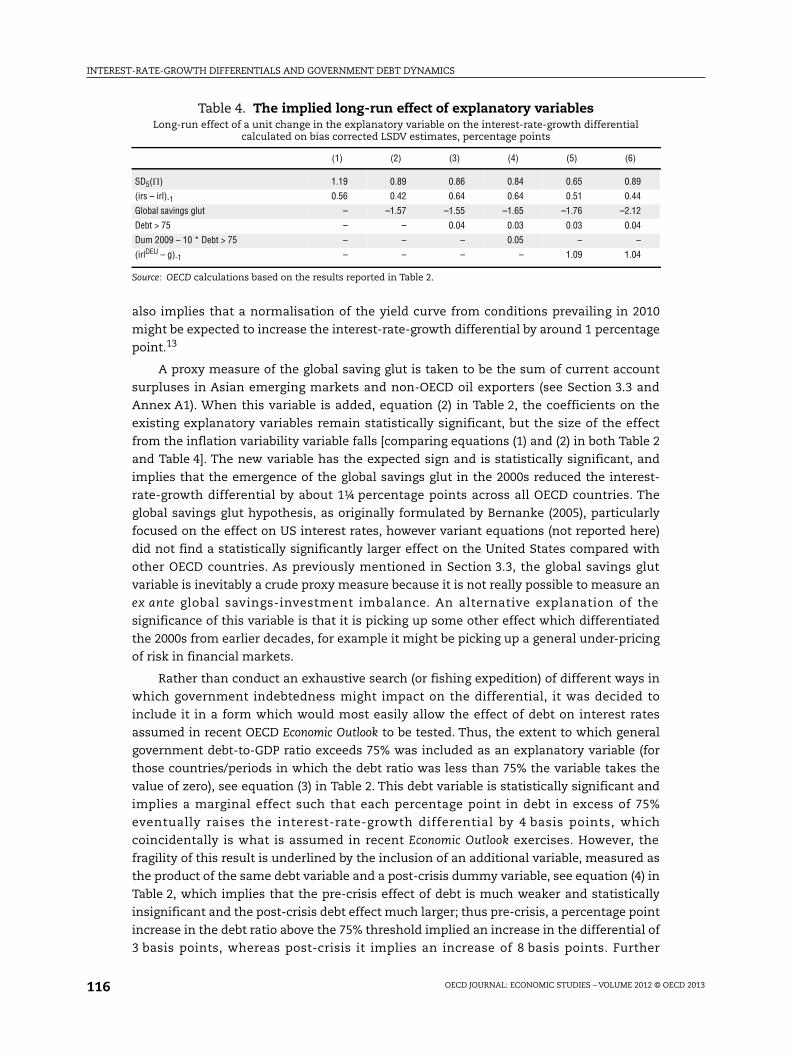
A proxy measure of the global saving glut is taken to be the sum of current account

surpluses in Asian emerging markets and non-OECD oil exporters (see Section 3.3 and

Annex A1). When this variable is added, equation (2) in Table 2, the coefficients on the

existing explanatory variables remain statistically significant, but the size of the effect

from the inflation variability variable falls [comparing equations (1) and (2) in both Table 2

and Table 4]. The new variable has the expected sign and is statistically significant, and

implies that the emergence of the global savings glut in the 2000s reduced the interest-

rate-growth differential by about 1¼ percentage points across all OECD countries. The

global savings glut hypothesis, as originally formulated by Bernanke (2005), particularly

focused on the effect on US interest rates, however variant equations (not reported here)

did not find a statistically significantly larger effect on the United States compared with

other OECD countries. As previously mentioned in Section 3.3, the global savings glut

variable is inevitably a crude proxy measure because it is not really possible to measure an

ex ante global savings-investment imbalance. An alternative explanation of the

significance of this variable is that it is picking up some other effect which differentiated

the 2000s from earlier decades, for example it might be picking up a general under-pricing

of risk in financial markets.

Rather than conduct an exhaustive search (or fishing expedition) of different ways in

which government indebtedness might impact on the differential, it was decided to

include it in a form which would most easily allow the effect of debt on interest rates

assumed in recent OECD Economic Outlook to be tested. Thus, the extent to which general

government debt-to-GDP ratio exceeds 75% was included as an explanatory variable (for

those countries/periods in which the debt ratio was less than 75% the variable takes the

value of zero), see equation (3) in Table 2. This debt variable is statistically significant and

implies a marginal effect such that each percentage point in debt in excess of 75%

eventually raises the interest-rate-growth differential by 4 basis points, which

coincidentally is what is assumed in recent Economic Outlook exercises. However, the

fragility of this result is underlined by the inclusion of an additional variable, measured as

the product of the same debt variable and a post-crisis dummy variable, see equation (4) in

Table 2, which implies that the pre-crisis effect of debt is much weaker and statistically

insignificant and the post-crisis debt effect much larger; thus pre-crisis, a percentage point

increase in the debt ratio above the 75% threshold implied an increase in the differential of

3 basis points, whereas post-crisis it implies an increase of 8 basis points. Further

Table 4. The implied long-run effect of explanatory variablesLong-run effect of a unit change in the explanatory variable on the interest-rate-growth differential

calculated on bias corrected LSDV estimates, percentage points

(1) (2) (3) (4) (5) (6)

SD5() 1.19 0.89 0.86 0.84 0.65 0.89

(irs – irl)-1 0.56 0.42 0.64 0.64 0.51 0.44

Global savings glut – –1.57 –1.55 –1.65 –1.76 –2.12

Debt > 75 – – 0.04 0.03 0.03 0.04

Dum 2009 – 10 * Debt > 75 – – – 0.05 – –

(irlDEU – g)-1 – – – – 1.09 1.04

Source: OECD calculations based on the results reported in Table 2.



regressions, not reported here, suggest that the increased effect from indebtedness in the

post-crisis period is mostly accounted for by the euro area countries. This result is

consistent with the finding that interest rate spreads may be more sensitive to perceived

imbalances within a currency union because of the inability of individual member

countries to freely issue currency to finance increased indebtedness (de Grauwe, 2011).

A final pair of regressions explore the effect that European Monetary Union had on the

interest-rate-growth differential (Table 2, equations 5 and 6). Given the evidence that EMU

led to a striking convergence of long-term interest rates (Figure 7), a lagged variable in the

differential between German long-term interest rates and own-country growth for all EMU

countries in the sample over the period 1998 to 2008 was included. The long-run coefficient

on this new variable is close to unity, implying that German long rates were a powerful

attractor for long-term interest rates in other EMU countries over the period 1998-2008. The

fit of this equation is included by excluding the influence of the inflation variability, global

savings glut and debt variables for non-German EMU countries over the period 1998-2008.

Arguably the influence of lower inflation variability and the global savings glut variable is

already included in German long-term interest rates and so if this is an attractor for other

EMU long-term rates there is no need to include the effect separately. The improved

significance of the debt variable, when EMU countries are excluded for the period

1998-2008, further suggests that the effect of government indebtedness on fiscal risk

premia was suspended for these countries over the period 1998-2008, an effect which is

more difficult to rationalise.

Also of interest is that the long-run effect of most of the explanatory variables for non-

EMU countries is little affected by these EMU variant equations (Table 4), with the possible

exception of the effect of the global savings glut variable which has a slightly larger and

more statistically significant effect.

Notes

1. The focus of this paper is on explaining the interest-rate-growth differential of some OECDeconomies since 1980. The corresponding differential for developing countries is typically muchlower, and usually negative, which mainly appears to be the consequence of financial repression(Escolano et al., 2011 and IMF, 2011a). The experience of OECD countries prior to 1980 is excludedfrom the empirical analysis because the widespread use of financial repression measures(Reinhart and Sbrancia, 2011) coupled with the large inflation shades of the 1970s suggests that theexperience of interest rates prior to 1980 will not be informative of the experience since then.

2. An illustration of the lack of any analytical foundation for projecting the differential is that, for thepurpose of making medium-term fiscal projections to 2030 for the “Advanced Economies”, the IMFassume in their regular Fiscal Monitor publication that “up to 2015, an interest-rate-growthdifferential of 0 percentage points …, broadly in line with WEO assumptions, and 1 percentagepoint afterwards, regardless of country-specific circumstances” (IMF, 2011b), yet there is little or nojustification or discussion of the basis for this assumption despite its importance.

3. This ignores stock-flow adjustments which have been particularly important over the crisis period,see IMF, 2011b.

4. The baseline projection is consistent with a rise in the interest-rate-growth differential to justunder 2 percentage points by 2026. The lower debt path would be consistent with an interest-rate-growth differential of around zero percentage points which is similar to that experienced by theUnited States over the last decade, whereas the high debt path would be consistent with adifferential rising to about 4 percentage points.

5. The sharp drop in forward rates in the United Kingdom on the day the Bank of England wasgranted operational independence, is also cited as further evidence of this effect (Wright, 2011).



6. The slope of the yield curve is also a well-known predictor of GDP growth, however this effect isnot captured in the regressions estimated here because GDP growth in the interest-rate-growthdifferential is de-trended.

7. See Box 4.5 in OECD (2010) for a selective survey.

8. Égert (2010) finds that the difference between short-term and long-term interest rates appear to bea non-linear function of public debt for the G7 countries (excluding Japan) in recent years. Theestimation results indicate a 4 basis point increase in long-term rates relative to short-term ratesfor each percentage point of GDP in public debt above 76%. Laubach (2009) focuses on the UnitedStates and finds that long-term yields increase about 25 basis points per percentage point increasein the projected deficit-to-GDP ratio, and 3 to 4 basis points per percentage point increase in thedebt-to-GDP ratio.

9. In May 1998, the 11 countries that would initially participate in EMU were selected and, inJune 1998, the ECB was created.

10. The panel is unbalanced, because there are some countries for which data are not complete overthe full sample period. The results for individual country regressions are not presented as in manycases estimated coefficients were statistically insignificant. Further details are given in Annex A1.

11. Indeed, a simple least squares estimation with country fixed effects (with no correction for thepresence of a lagged dependent variable) gives similar results, as reported in Annex A2, to thosereported in the main body of the paper based on the estimator proposed by Bruno (2005).

12. The results are robust to using different measures of inflation, such as ones based on theConsumer Price Index or Private Consumption Expenditure Deflator. For further details on thevariables used in the estimation see Annex A1.

13. This calculation assumes that in the absence of cyclical influences, long-term interest rates wouldbe expected to exceed short-term rates by about ½ percentage point because of a term premium.

References

Baltagi, B. and J. Griffin (1997), “Pooled Estimators vs their Heterogeneous Counterparts in the Contextof Dynamic Demand for Gasoline”, Journal of Econometrics, Vol. 77.

Beffy, P., P. Ollivaud, P. Richardson and F. Sédillot (2006), “New OECD Methods for Supply-Side andMedium-Term Assessments: A Capital Services Approach”, OECD Economics Department WorkingPaper, No. 482.

Bernanke, B. (2005), “The Global Savings Glut and the US Current Account Deficit”, speech delivered atthe Sandridge Lecture, Virginia Association of Economists, Richmond, Va, 10 March.

Bernanke, B. (2007), “The Global Imbalances: Recent Developments and Prospects”, speech delivered atthe Bundesbank Lecture, Berlin, Germany, 11 September.

Bernanke, B., C. Bertaut, L. Pounder DeMarco and S. Kamin (2011), “International Capital Flows and theReturn to Safe Assets in the United States, 2003-7”, Board of Governors of the Federal ReserveSystem, International Finance Discussion Papers, No. 1014, February.

Bruno, G. (2005), “Approximating the Bias of the LSDV Estimator for Dynamic Unbalanced Panel DataModels”, Economic Letters, Vol. 87.

Dobbs, R., et al. (2010), “Farewell to Cheap Capital? The Implications of Long-Term Shifts in GlobalInvestment and Savings”, McKinsey Global Institute, December.

De Grauwe, P. (2011), “The Governance of a Fragile Eurozone”, CEPS Working Document, No. 346, May.

Égert, B. (2010), “Fiscal Policy Reaction to the Cycle in the OECD: Pro- or Counter-Cyclical?”, OECDEconomics Department Working Papers, No. 763.

Escolano, J., A. Shabunina and J. Woo (2011), “The Puzzle of Persistently Negative Interest Rate-GrowthDifferentials: Financial Repression or Income Catch-Up?”, IMF Working Paper No. 11/260.

Gagnon, J, M. Raskin, J. Remache and B. Sack (2011), “The Financial Market Effects of the FederalReserve’s Large-Scale Asset Purchases”, International Journal of Central Banking, Vol. 7, No. 1, March.

Haugh, D., P. Ollivaud and D. Turner (2009), “What Drives Sovereign Risk Premiums? An Analysis ofRecent Evidence from the Euro Area”, OECD Economics Department Working Papers, No. 718.

IMF (2011a), “Chapter 3-Shocks to the baseline Fiscal Outlook”, IMF Fiscal Monitor, Washington, April.



IMF (2011b), IMF Fiscal Monitor, Washington, September.

Joyce, M., A. Lasaosa, I. Stevens and M. Tong (2011), “The Financial Market Impact of QuantitativeEasing”, International Journal of Central Banking, Vol. 7, No. 3, pp. 113-61.

Laubach, T. (2009), “New Evidence on the Interest Rate Effects of Budget Deficits and Debt”, Journal ofthe European Economic Association, Vol. 7.

Nickell, S. (1981), “Biases in Dynamic Models with Fixed Effects”, Econometrica, Vol. 49.

OECD (2010), “Chapter 4-Fiscal Consolidation: Requirements, Timing, Instruments and InstitutionalArrangements”, OECD Economic Outlook, Vol. 2010/2, No. 88, Paris.

OECD (2011), “Chapter 4-Medium and Long-Term Developments: Challenges and Risks”, OECDEconomic Outlook, No. 89, May.

Reinhart, C. and K. Rogoff (2010), “Growth in a Time of Debt”, American Economic Review, Vol. 100.

Reinhart, C.M., J.F. Kirkegaard and M.B. Sbrancia (2011), “Financial Repression Redux”, Finance &Development, Vol. 48, No. 1, June.

Reinhart, C.M. and M.B. Sbrancia (2011), “The Liquidation of Government Debt”, National Bureau ofEconomic Research, NBER Working Papers, No. 16893.

Wright, J. (2011), “Term Premia and Inflation Uncertainty: Empirical Evidence from an InternationalPanel Dataset”, American Economic Review, Vol. 101.



ANNEX A1

Data description

The data used in this article cover selected OECD member countries over the period

1980-2010. These countries were selected to maximise the time span of the panel dataset

so that the maximum number of observations per variable would be 713. However, due to

the gaps in the data for some countries, particularly Greece and Iceland, the effective

number of observations used in each regression is slightly lower. The exact country

coverage of the variables is presented in Table A1.1.

Most of the data used in this article are taken from the recently published OECD

Economic Outlook Database No. 89, released in June 2011. Data used to construct the measure

of the “global savings glut” are extracted from the IMF World Economic Outlook (WEO)

database, released in September 2011.

Although various information on the variables used in the empirical analysis are

provided in different sections of the main text, some extra details on the definition and

construction of these variables are given below.

The simple model, corresponding to equation (1) in Table 2, includes the following

variables:

● The interest-rate-growth differential as dependent variable defined as the difference between

the levels of the interest rate on 10-year government bonds and nominal potential GDP

growth.* In the case of Norway, potential GDP estimates refer to the mainland economy,

Table A1.1. Details on data availability

Variable Start date End date Exceptions to the starting date

Interest rate – growth differential (irl – g)tdependentvariable 1980 2010

Portugal and New Zealand (1981), Switzerland (1982),Korea (1983), Greece (1994), Iceland (1992)

Short-term interest rate minus Long-term interestrate (irs – irl)t 1980 2010

Denmark (1981), Sweden (1983), Ireland (1985),Greece (1994), Iceland (1993), Korea (1992)

Standard deviation of inflation SD5()t 1980 2010 Greece (1997)

Global savings glut 1980 2010

Debt 751980 2010

Australia (1988), New Zealand (1993), Greeceand Portugal (1995), Ireland, Iceland (1998)

German long-term interest rates – own-country growthdifferential (irl DEU – g)t for non-German Euro areacountries 1980 2010 Portugal (1981) and Greece (1994)

* Potential growth is estimated using a production function approach as described in Beffy et al., 2006.



while in the case of Germany, a long time series for potential growth is explicitly

constructed by splicing the growth rates of nominal potential GDP from 1991 on those of

West Germany.

● Inflation volatility is measured as a five-year standard deviation of inflation, where the

latter refers to the change in the GDP deflator.

● The slope of the yield curve is calculated as the difference between short-term interest

rates (generally three-month Treasury bill rate) and long-term interest rates on 10-year

Treasury bonds.

This model is subsequently extended with the inclusion of one or more of the

following variables:

● A proxy measure of the global savings glut in equation (2) in Table 2, obtained by

combining current account surpluses of Asian emerging economies and main oil

exporting countries expressed as percentage of world GDP. Specifically, the two country

groups selected from the WEO were “Developing Asia” and “Middle East and North

Africa” (for more details on the groups composition see Table A1.2).

● A variable measuring high government indebtedness is included in equation (3) of

Table 2, and constructed for each country as the excess of the general government

debt-to-GDP ratio when this share is above the threshold of 75% of GDP, and zero

otherwise.

● A dummy variable taking value unity in the post-crisis years of 2009 and 2010 and zero

elsewhere is used in equation (4) of Table 2 to construct the interaction term that allows

for the testing of a differential effect from debt in the post-crisis years.

● A lagged variable measuring the differential between German long-term interest rates

and other own-country growth in other EMU countries over the period 1998-2008 is

considered in equation (5), Table 2.

● Finally, a dummy variable taking value unity for Euro area countries-with the exception

of Germany-from 1998 to 2008 included and zero elsewhere, is used to exclude the

influence of inflation volatility, global savings glut and debt variable for non-Germany

EMU countries over that specific period from equation (6) in Table 2.

Table A1.2. List of countries composing the different aggregates consideredin the empirical analysis

Country aggregate Component countries

Selected OECD countries Australia, Austria, Belgium, Canada, Denmark, Finland, France, Germany, Greece, Iceland, Ireland, Italy,Japan, Korea, Netherlands, New Zealand, Norway, Portugal, Spain, Sweden, Switzerland, United Kingdom,United States.

G7 Canada, France, Germany, Italy, Japan, United Kingdom, United States.

Selected EMU countries Austria, Belgium, Finland, France, Greece, Ireland, Italy, The Netherlands, Portugal, Spain.

Developing Asia Afghanistan, Bangladesh, Bhutan, Brunei, Cambodia, China, Fiji, India, Indonesia, Kiribati, Lao People’sDemocratic Republic, Malaysia, Maldives, Myanmar, Nepal, Pakistan, Papua New Guinea, Philippines,Samoa, Solomon Islands, Sri Lanka, Thailand, Democratic Republic of Timor-Leste, Tonga, Tuvalu, Vanuatu,Vietnam.

Middle East and North Africa Algeria, Bahrain, Djibouti, Egypt, Islamic Republic of Iran, Iraq, Jordan, Kuwait, Lebanon, Libya, Mauritania,Morocco, Oman, Qatar, Saudi Arabia, Sudan, Syrian Arab Republic, Tunisia, United Arab Emirates,Republic of Yemen.



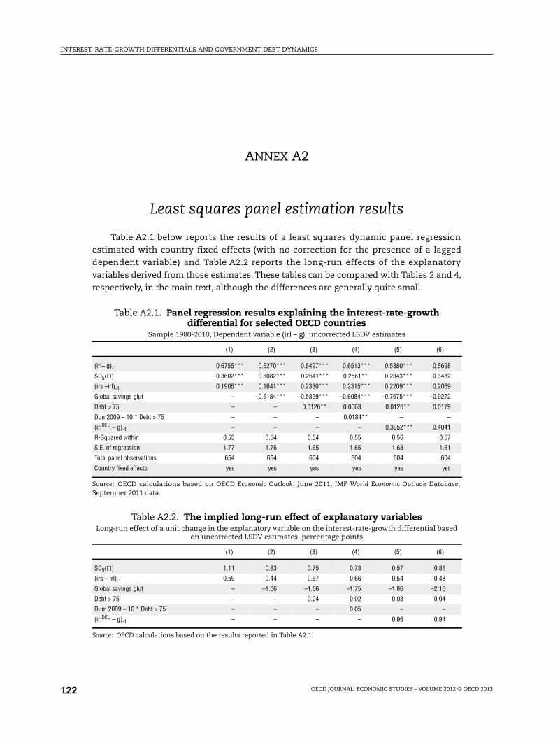
ANNEX A2

Least squares panel estimation results

Table A2.1 below reports the results of a least squares dynamic panel regression

estimated with country fixed effects (with no correction for the presence of a lagged

dependent variable) and Table A2.2 reports the long-run effects of the explanatory

variables derived from those estimates. These tables can be compared with Tables 2 and 4,

respectively, in the main text, although the differences are generally quite small.

Table A2.1. Panel regression results explaining the interest-rate-growthdifferential for selected OECD countries

Sample 1980-2010, Dependent variable (irl – g), uncorrected LSDV estimates

(1) (2) (3) (4) (5) (6)

(irl– g)-1 0.6755*** 0.6270*** 0.6497*** 0.6513*** 0.5880*** 0.5698

SD5() 0.3602*** 0.3082*** 0.2641*** 0.2561** 0.2343*** 0.3482

(irs –irl)-1 0.1906*** 0.1641*** 0.2330*** 0.2315*** 0.2209*** 0.2069

Global savings glut – –0.6184*** –0.5829*** –0.6084*** –0.7675*** –0.9272

Debt > 75 – – 0.0126** 0.0063 0.0126** 0.0179

Dum2009 – 10 * Debt > 75 – – – 0.0184** – –

(irlDEU – g)-1 – – – – 0.3952*** 0.4041

R-Squared within 0.53 0.54 0.54 0.55 0.56 0.57

S.E. of regression 1.77 1.76 1.65 1.65 1.63 1.61

Total panel observations 654 654 604 604 604 604

Country fixed effects yes yes yes yes yes yes

Source: OECD calculations based on OECD Economic Outlook, June 2011, IMF World Economic Outlook Database,September 2011 data.

Table A2.2. The implied long-run effect of explanatory variablesLong-run effect of a unit change in the explanatory variable on the interest-rate-growth differential based

on uncorrected LSDV estimates, percentage points

(1) (2) (3) (4) (5) (6)

SD5() 1.11 0.83 0.75 0.73 0.57 0.81

(irs – irl)-1 0.59 0.44 0.67 0.66 0.54 0.48

Global savings glut – –1.66 –1.66 –1.75 –1.86 –2.16

Debt > 75 – – 0.04 0.02 0.03 0.04

Dum 2009 – 10 * Debt > 75 – – – 0.05 – –

(irlDEU – g)-1 – – – – 0.96 0.94

Source: OECD calculations based on the results reported in Table A2.1.

and government debt dynamics interest-rate-growth ... · 1. the importance of the...

Documents