The N − k Problem in Power Grids: New Models, Formulations

and Computation1

Daniel Bienstock and Abhinav Verma

Columbia University

New York

May 2008

Abstract

Given a power grid modeled by a network together with equations describing the powerflows, power generation and consumption, and the laws of physics, the so-called N − k problemasks whether there exists a set of k or fewer arcs whose removal will cause the system to fail.We present theoretical results and computation involving two optimization algorithms for thisproblem.

1 Introduction

Recent large-scale power grid failures have highlighted the need for effective computational toolsfor analyzing vulnerabilities of electrical transmission networks. Blackouts are extremely rare, buttheir consequences can be severe. Recent blackouts had, as their root cause, an exogenous damagingevent (such as a storm) which developed into a system collapse even though the initial quantity ofdisabled power lines was small.

As a result, a problem that has gathered increasing importance is what might be termed thevulnerability evaluation problem: given a power grid, is there a small set of power lines whoseremoval will lead to system failure? Here, “smallness” is parameterized by an integer k, and indeedexperts have called for small values of k (such as k = 3 or 4) in the analysis. Additionally, an explicitgoal in the formulation of the problem is that the analysis should be agnostic: we are interestedin rooting out small, “hidden” vulnerabilities of a complex system which is otherwise quite robust;as much as possible the search for such vulnerabilities should be devoid of assumptions regardingtheir structure.

This problem is not new, and researchers have used a variety of names for it: network in-terdiction, network inhibition and so on, although the “N - k problem” terminology is commonin the industry (where “N” is the number of arcs). We will provide a more complete review ofthe (rather extensive) literature later on; the core central theme is that the N − k problem is veryhighly intractable, even for small values of k – the pure enumeration approach is simply impractical.In addition to the combinatorial explosion, another significant difficulty is the need to model thelaws of physics governing power flows in a sufficiently accurate and yet computationally tractablemanner: power flows are much more complex than “flows” in traditional applications.

A critique that has been leveled against optimization-based approaches to the N − k problemis that they tend to focus on large values of k, say k = 8. When k is large the problem tendsto become easier, but on the other hand the argument can be made that the cardinality of theattack is unrealistically large. At the other end of the spectrum lies the case k = 1, which can beaddressed by enumeration but may not yield useful information. The middle range, 2 ≤ k ≤ 5, isboth relevant and difficult, and is our primary focus.

In this paper we take an approach based on strict optimization. We present results usingtwo models. The first (Section 2.1) is a new linear mixed-integer programming formulation thatexplicitly models a “game” between a fictional attacker seeking to disable the network, and acontroller who tries to prevent a collapse by selecting which generators to operate and adjustinggenerator outputs and demand levels. As far as we can tell, the problem we consider here is

1Partially funded by NSF award 0521741

1

more general than has been previously studied in the literature; nevertheless our approach yieldspracticable solution times for larger instances than previously studied.

The second model (Section 3) is given by a new, continuous nonlinear programming formulationwhose goal is to capture, in a compact way, the interaction between the underlying physics and thenetwork structure. While both formulations provide substantial savings over the pure enumerationalapproach, the second formulation appears particularly effective and scalable; enabling us to handlein an optimization framework models an order of magnitude larger than those we have seen in theliterature.

1.0.1 Previous work on vulnerability problems

There is a large amount of prior work on optimization methods applied to blackout-related problems.[20] includes a fairly comprehensive survey of recent work.

Typically work has focused on identifying a small set of arcs whose removal (to model completefailure) will result in a network unable to deliver a minimum amount of demand. A problem of thistype can be solved using mixed-integer programming techniques techniques, see [2], [21], [3]. Wewill review this work in more detail below (Section 2.0.6). Generally speaking, the mixed-integerprograms to be solved can prove quite challenging.

A different line of research on vulnerability problems focuses on attacks with certain structuralproperties, see [6], [20]. An example of this approach is used in [20]. Here, as an approximationto the N − k problem with AC power flows, the authors formulate a linear mixed-integer programto solve the following combinatorial problem: remove a minimum number of arcs, such that in theresulting network there is a partition of the nodes into two sets, N1 and N2, such that

D(N1) + G(N2) + cap(N1, N2) ≤ Qmin.

Here D(N1) is the total demand in N1, G(N2) is the total generation capacity in N2, cap(N1, N2) isthe total capacity in the (non-removed) arcs between N1 and N2, and Qmin is a minimum amountof demand that needs to be satisfied. The quantity in the left-hand side in the above expressionis an upper-bound on the total amount of demand that can be satisfied – the upper-bound can bestrict because under power flaw laws it may not be attained.

Thus this is an approximate model that could underestimate the effect of an attack (i.e. thealgorithm may produce attacks larger than strictly necessary). On the other hand, methods ofthis type bring to bear powerful mathematical tools, and thus can handle larger problems thanalgorithms that rely on generic mixed-integer programming techniques. Our method in Section 3can also be viewed as an example of this approach.

Finally, we mention that the most sophisticated models for the behavior of a grid under stressattempt to capture the multistage nature of blackouts, and are thus more comprehensive than thestatic models considered above and in this paper. See, for example, [9]-[12], and [5].

1.0.2 Power Flows

Here we provide a brief introduction to the so-called linearized, or DC power flow model. For thepurposes of our problem, a grid is represented by a directed network N , where:

• Each node corresponds to a “generator” (i.e., a supply node), or to a “load” (i.e., a demandnode), or to a node that neither generates nor consumes power. We denote by G the set ofgenerator nodes.

• If node i corresponds to a generator, then there are values 0 ≤ Pmini ≤ Pmax

i . If the generatoris operated, then its output must be in the range [Pmin

i , Pmaxi ]; if the generator is not operated,

then its output is zero. In general, we expect Pmini > 0.

• If node i corresponds to a demand, then there is a value Dnomi (the “nominal” demand value

at node i). We will denote the set of demands by D.

2

• The arcs of N represent power lines. For each arc (i, j), we are given a parameter xij > 0(the resistance) and a parameter uij (the capacity).

Given a set C of operating generators, a power flow is a solution to the system of constraints givennext. In this system, for each arc (i, j), we use a variable fij to represent the (power) flow on (i, j)– possibly fij < 0, in which case power is effectively flowing from j to i. In addition, for each nodei we will have a variable θi (the “phase angle” at i). Finally, if i is a generator node, then we willhave a variable Pi, while if i represents a demand node, we will have a variable Di. The constraintsare:

∑

(i,j)∈δ+(i)

fij −∑

(j,i)∈δ−(i)

fji =

Pi i ∈ C−Di i ∈ D

0 otherwise(1)

θi − θj + xijfij = 0 ∀(i, j) (2)

|fij | ≤ uij, ∀(i, j) (3)

Pmini ≤ Pi ≤ Pmax

i ∀i ∈ C (4)

0 ≤ Dj ≤ Dnomj ∀j ∈ D (5)

We will denote this system by P (N , C). Constraint (1) models flow conservation, while (4) and (5)describe generator and demand node bounds. Optionally, one may impose additional constraints,in particular bounds on the θi or on the quantities |θi − θj| (over the arcs (i, j)).

1.0.3 Basic results

A useful property satisfied by the linearized model is summarized by the following result which isnot difficult to prove.

Lemma 1.1 Let C be given, and suppose N is connected. Then for any choice of nonnegativevalues Pi (for i ∈ C) and Di (for i ∈ D) such that

∑

i∈CPi =

∑

i∈DDi, (6)

system (1)-(2) has a unique solution in the fij; the solution is also unique in the θi − θj (over thearcs (i, j)).

Remark 1.2 We stress that Lemma 1.1 concerns the subsystem of P (N , C) consisting of (1) and(2). In particular, the “capacities” uij play no role in the determination of solutions.

When the network is not connected Lemma 1.1 can be extended by requiring that (6) hold for eachcomponent.

Definition 1.3 Let (f, θ, P,D) be feasible a solution to P (N , C). The throughput of (f, θ, P,D)is defined as

∑i∈DDi∑

i∈DDnomi

. (7)

The throughput of N is the maximum throughput of any feasible solution to P (N , C).

3

1.0.4 DC and AC power flows

Constraint (2) is reminiscent of Ohm’s equation – in a direct current (DC) network (2) preciselyrepresents Ohm’s equation. In the case of an AC network (the relevant case when dealing withpower grids) (2) only approximates a complex system of nonlinear equations (see [1]). The issueof whether to use an the more exact nonlinear formulation, or the approximate DC formulation,is rather thorny. On the one hand, the linearized formulation certainly is an approximation only.On the other hand, the AC formulation can prove intractable or otherwise inappropriate (e.g. theformulation may have multiple solutions), and, we stress, is itself in any case an approximate modelof the underlying physics.

For these reasons, studies that require multiple power flow computations tend to rely on the lin-earized formulation. This will be the approach we take in this paper, though some of our techniquesextend directly to the AC model and this will remain a topic for future research. An approachsuch as ours can therefore be criticized because it relies on an ostensibly approximate model; onthe other hand we are able to focus more explicitly on the basic combinatorial complexity thatunderlies the N−k problem. In contrast, an approach that uses the AC model would have a betterrepresentation of the physics, but at the cost of not being able to tackle the combinatorial com-plexity quite as effectively, for the simple reason that the theory and computational machinery forlinear programming are far more mature, effective and scalable than those for nonlinear, nonconvexoptimization. In summary, both approaches present limitations and benefits. In this paper, ourbias is toward explicitly handling the combinatorial nature of the problem.

A final point that we would like to stress is that whether we use the AC or DC power flow model,the resulting problems have a far more complex structure than (say) traditional single- or multi-commodity flow models because of side side-constraints such as (2). Constraints of this type giverise to counter-intuitive behavior reminiscent of Braess’s Paradox [8].

2 The “N - k” problem

Let N be a network with n nodes and m arcs representing a power grid. We denote the set of arcsby E and the set of nodes by V . A fictional attacker wants to remove a small number of arcs fromN in order to maximize damage. Somewhat informally (and, as it turns out, incompletely), thegoal of the attacker is that in the resulting network all feasible flows should have low throughput.At the same time, a controller is operating the network; the controller responds to an attack byappropriately choosing the set C of operating generators, their output levels, and the demands D i,so as to feasibly obtain high throughput.

Thus, the attacker seeks to defeat all possible courses of action by the controller, in other words,we are modeling the problem as a Stackelberg game between the attacker and the controller, wherethe attacker moves first. To cast this in a precise way we will use the following definition. We let0 ≤ Tmin ≤ 1 be a given value.

Definition 2.1 Given a network N ,

• An attack A is a set of arcs removed by the attacker.

• Given an attack A, the surviving network N −A is the subnetwork of N consisting of thearcs not removed by the attacker.

• A configuration is a set C of generators.

• We say that an attack A defeats a configuration C, if either (a) the maximum throughput ofany feasible solution to P (N − A, C) is strictly less than Tmin, or (b) no feasible solutionto P (N − A, C) exists. Otherwise we say that C defeats A.

• We say that an attack is successful, if it defeats every configuration.

4

• The min-cardinality attack problem consists in finding a successful attack A with |A|minimum.

Our primary focus will be on the min-cardinality attack problem. Before proceeding further wewould like to comment on our model, specifically on the parameter Tmin. In a practical use of themodel, one would wish to experiment with different values for Tmin – for the simple reason that anattack A which is not successful for a given choice for Tmin could well be successful for a slightlylarger value; e.g. no attack or cardinality 3 or less exists that reduces demand by 31%, and yetthere exists an attack of cardinality 3 that reduces satisfied demand by 30%. In other words, theminimum cardinality of a successful attack could vary substantially as a function of T min.

Given this fact, it might appear that a better approach to the power grid vulnerability problemwould be to leave out the parameter Tmin entirely, and instead redefine the problem to that offinding a set of k or fewer arcs to remove, so that the resulting network has minimum throughput(here, k is given). We will refer to this as the budget-k min-throughput problem. However, there arereasons why this latter problem is less attractive than the min-cardinality problem.

(a) Clearly, in a sense, the min-cardinality and min-throughput problems are duals of each other.A modeler considering the min-throughput problem would want to run that model multipletimes, because given k, the value of the budget-k min-throughput problem could be muchsmaller than the value of the budget-(k + 1) min-throughput problem. For example, it couldbe the case that using a budget of k = 2, the attacker can reduce throughput by no morethan 5%; but nevertheless with a budget of k = 3, throughput can be reduced by e.g. 50%. Inother words, even if a network is “resilient” against attacks of size ≤ 2, it might neverthelessprove very vulnerable to attacks of size 3. For this reason, and given that the models of grids,power flows, etc., are rather approximate, a practitioner would want to test various valuesof k – this issue is obviously related to what percentage of demand loss would be consideredtolerable, in other words, the parameter Tmin.

(b) From an operational perspective it should be straightforward to identify reasonable values forthe quantity Tmin; whereas the value k is more obscure and bound to models of how muchpower the adversary can wield.

(c) Because of a subtlety that arises from having positive quantities Pmini , explained next, it

turns out that the min-throughput problem is significantly more complex and is difficult toeven formulate in a compact manner.

We will now expand on (c). One would expect that when a configuration C is defeated by an attackA, it is because only small throughput solutions are feasible in N −A. However, because the lowerbounds Pmin

i are in general strictly possible, it may also be the case that no feasible solution toP (N − A, C) exists.

Example 2.2 Consider the following example on a network N with three nodes, where

1. Nodes 1 and 2 represent generators; Pmin1 = 2, Pmax

1 = 4, Pmin2 = 0, and Pmax

2 = 4,

2. Node 3 is a demand node with Dnom3 = 6. Furthermore, Tmin = 1/2.

3. There are three arcs; arc (1, 2) with x12 = 1 and u12 = 3, arc (2, 3) with x23 = 1 and u23 = 5,and arc (1, 3) with x13 = 1 and u13 = 1.

When the network is not attacked, the following solution is feasible: P1 = P2 = 3, D3 = 6, f12 = 0,f13 = f23 = 3, θ1 = θ2 = 0, θ3 = −3. This solution has throughput 100%. On the other hand,consider the attack A consisting of the single arc (1, 3), and suppose we choose the configurationC = {1, 2} (i.e. we operate both generators). Since Pmin

1 > u12, P (N − A, C) has no feasiblesolution, and A defeats C (in spite of the fact that we can still meet 100% of the demand).

Likewise, A defeats the configuration where we only operate generator 1. Thus, A is successful ifand only if it also defeats the configuration where we only operate generator 2, which it does not sincein that configuration we can feasibly send up to four units of flow on (2, 3) and T min = 1/2 < 4/6.

5

As the example highlights, it is important to understand how an attack A can defeat a particularconfiguration C. It turns out that there are three different ways for this to happen.

(i) Consider a partition of the nodes of N into two classes, N 1 and N2. Write

Dk =∑

i∈D∩Nk

Dnomi , k = 1, 2, and (8)

P k =∑

i∈C∩Nk

Pmaxi , k = 1, 2, (9)

e.g. the total (nominal) demand in N1 and N2, and the maximum power generation in N1

and N2, respectively. The following condition, should it hold, would guarantee that A defeatsC:

Tmin∑

j∈DDnom

j −min{D1, P 1} −min{D2, P 2} >∑

(i,j)/∈A : i∈N1, j∈N2

uij +

∑

(i,j)/∈A : i∈N2, j∈Nj

uij. (10)

To understand this condition, note that for k = 1, 2, min{Dk, P k} is the maximum demandwithin Nk that could possibly be met using power flows that do not leave N k. Consequentlythe left-hand side of (10) is a lower bound on the amount of flow that must travel betweenN1 and N2, whereas the right-hand side of (10) is the total capacity of arcs between N 1 andN2 under attack A. In other words, condition (10) amounts to a mismatch between demandand supply. A special case of (10) is that where in N −A there are no arcs between N 1 andN2, i.e. the right-hand side of (10) is zero.

(ii) Consider a partition of the nodes of N into two classes, N 1 and N2, such that in N −A thereare no arcs between N 1 and N2. Then attack A defeats C if

∑

iD∩∈N1

Dnomi <

∑

i∈C∩N1

Pmini , (11)

i.e., the minimum power output within N 1 exceeds the maximum demand within N 1. Notethat (ii) may apply even if (i) does not.

(iii) Even if (i) and (ii) do not hold, it may still be the case that the system (1)-(5) does not admita feasible solution. To put it differently, suppose that for every choice of demand values0 ≤ Di ≤ Dnom

i (for i ∈ D) and supply values Pmini ≤ Pi ≤ Pmax

i (for i ∈ C) such that∑i∈C Pi =

∑i∈DDi the unique solution to system (1)-(2) in network N −A (as per Lemma

1.1) does not satisfy the “capacity” inequalities |fij| ≤ uij for all arcs (i, j) ∈ N −A. ThenA defeats C. This is the most subtle case of all – it involves the interplay of flow conservationand Ohm’s law.

Note that in particular in case (ii), the defeat condition is unrelated to throughput. Never-theless, should case (ii) arise, it is clear that the attack has succeeded (against configuration C) –this makes the min-throughput problem difficult to model; our formulation for the min-cardinalityproblem, given in Section 2.1, does capture the three defeat criteria above.

From a practical perspective, it is important to handle models where the values P mini are pos-

itive. It is also important to model standby generators that are turned on when needed, and tomodel the turning off of generators that are unable to dispose of their minimum power output,post-attack. All these features arise in practice. Example 2.2 above shows that models wheregenerators cannot be turned off can exhibit unreasonable behavior. Of course, the ability to selectthe operating generators comes at a cost, in that in order to certify that an attack is successful weneed to evaluate, at least implicitly, a possibly exponential number of control possibilities.

6

As far as we can tell, most (or all) prior work in the literature does require that the controllermust always use the configuration G consisting of all generators. As the example shows, however,if the quantities Pmin

i are positive there may be attacks A such that P (N − A, G) is infeasible.Because of this fact, algorithms that rely on direct application of Benders’ decomposition or bilevelprogramming are problematic, and invalid formulations can be found in the literature.

Our approach works with general Pmin ≥ 0 quantities; thus, it also applies to the case wherewe always have Pmin

i = 0. In this case our formulation is simple enough that a commercial integerprogram solver can directly handle instances larger than previously reported in the literature.

2.0.5 Non-monotonicity

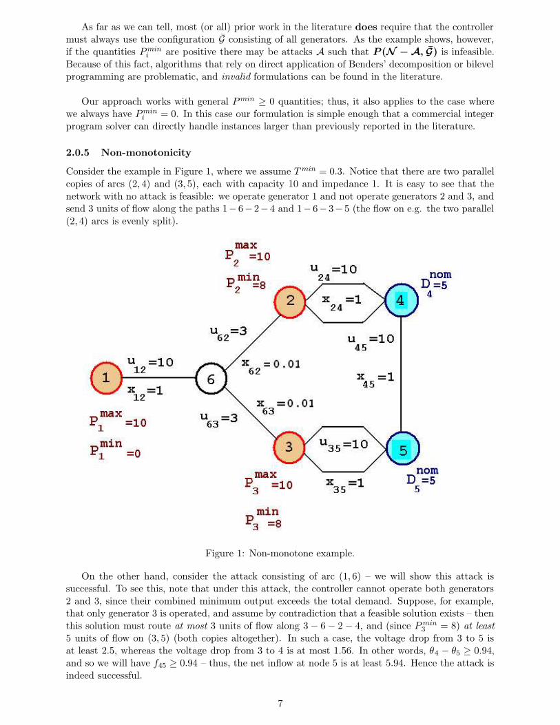
Consider the example in Figure 1, where we assume Tmin = 0.3. Notice that there are two parallelcopies of arcs (2, 4) and (3, 5), each with capacity 10 and impedance 1. It is easy to see that thenetwork with no attack is feasible: we operate generator 1 and not operate generators 2 and 3, andsend 3 units of flow along the paths 1− 6− 2− 4 and 1− 6− 3− 5 (the flow on e.g. the two parallel(2, 4) arcs is evenly split).

Figure 1: Non-monotone example.

On the other hand, consider the attack consisting of arc (1, 6) – we will show this attack issuccessful. To see this, note that under this attack, the controller cannot operate both generators2 and 3, since their combined minimum output exceeds the total demand. Suppose, for example,that only generator 3 is operated, and assume by contradiction that a feasible solution exists – thenthis solution must route at most 3 units of flow along 3− 6− 2 − 4, and (since Pmin

3 = 8) at least5 units of flow on (3, 5) (both copies altogether). In such a case, the voltage drop from 3 to 5 isat least 2.5, whereas the voltage drop from 3 to 4 is at most 1.56. In other words, θ4 − θ5 ≥ 0.94,and so we will have f45 ≥ 0.94 – thus, the net inflow at node 5 is at least 5.94. Hence the attack isindeed successful.

7

However, there is no successful attack consisting of arc (1, 6) and another arc. To see this, notethat if one of (2, 6), (3, 6) or (4, 5) are also removed then the controller can just operate one of thetwo generators 2, 3 and meet eight units of demand. Suppose that (say) one of the two copies of(3, 5) is removed (again, in addition to (1, 6)). Then the controller operates generator 2, sending2.5 units of flow on each of the two parallel (2, 4) arcs; thus θ2−θ4 = 2.5. The controller also routes3 units of flow along 2 − 6 − 3 − 5, and therefore θ2 − θ5 = 3.06. Consequently θ4 − θ5 = .56, andf45 = .56, resulting in a feasible flow which satisfies 4.44 units of demand at 4 and 3.56 units ofdemand at 5.

In fact, it is straightforward to show that no successful attack of of cardinality 2 exists – hencewe observe non-monotonicity.

By elaborating on the above, one can create examples with arbitrary patterns in the cardinalityof successful attacks. One can also generate examples that exhibit non-monotone behavior in re-sponse to controller actions. In both cases, the non-monotonicity can be viewed as a manifestationof the so-called “Braess’s Paradox” [8]. In the above example we can observe combinatorial sub-tleties that arise from the ability of the controller to choose which generators to operate, and fromthe lower bounds on output in operating generators. Nevertheless, it is clear that the critical corereason for the complexity is the interaction between voltages and flows, i.e. between “Ohm’s law”(2) and flow conservation (1) – the combinatorial attributes of the problem exercise this interac-tion. Thus, we view it as crucial that an optimization model address the interaction in an explicitmanner.

2.0.6 Brief review of previous work

The min-cardinality problem, as defined above, can be viewed as a bilevel program where both themaster problem and the subproblem are mixed-integer programs – the master problem correspondsto the attacker (who chooses the arcs to remove) and the subproblem to the controller (who choosesthe generators to operate). In general, such problems are extremely challenging. A recent general-purpose algorithm for such integer programs is given in [14].

Alternatively, each configuration of generators can be viewed as a “scenario”. In this senseour problem resembles a stochastic program, although without a probability distribution. Recentwork [17] considers a single commodity max-flow problem under attack by an interdictor with alimited attack budget; where an attacked arc is removed probabilistically, leading to a stochasticprogram (to minimize the expected max flow). A deterministic, multi-commodity version of thesame problem is given in [18].

Previous work on the power grid vulnerability models proper has focused on cases where eitherthe generator lower bounds Pmin

i are all zero, or all generators must be operated (the single config-uration case). Algorithms for these problems have either relied on heuristics, or on mixed-integerprogramming techniques, usually a direct use of Benders’ decomposition or bilevel programming.[2] considers a version of the min-throughput problem with Pmin

i = 0 for all generators i, andpresents an algorithm using Benders’ decomposition (also see references therein). They analyze theso-called IEEE One-Area and IEEE Two-Area test cases, with, respectively, 24 nodes and 38 arcs,and 48 nodes and 79 arcs. Also see [21].

[3] studies the IEEE One-Area test case, and allows Pmini > 0, but does not allow generators

to be turned off; the authors present a bilevel programming formulation which, unfortunately, isincorrect, due to reasons outlined above.

2.1 An algorithm for the min-cardinality problem

In this section we will describe an iterative algorithm for the min-cardinality attack problem. Thealgorithm iterates in Benders-like fashion, solving at each iteration two mixed-integer programs.Before describing the algorithm we need to introduce some notation and concepts.

8

Let A be a given attack. Suppose the controller attempts to defeat the attacker by choosinga certain configuration C of generators. Denote by zA the indicator vector for A, i.e. zAij = 1 iff(i, j) ∈ A. Then the controller needs to solve the following linear program:

KC(A) : tC(zA)

.= min t (12)

Subject to:

∑

(i,j)∈δ+(i)

fij −∑

(j,i)∈δ−(i)

fji =

Pi i ∈ G−Di i ∈ D

0 otherwise(13)

θi − θj + xijfij = 0 ∀ (i, j) /∈ A (14)

uij t − |fij | ≥ 0, ∀ (i, j) /∈ A (15)

fij = 0, ∀(i, j) ∈ A (16)

Pmini ≤ Pi ≤ Pmax

i ∀i ∈ C (17)

Pi = 0, ∀i ∈ G − C (18)

∑

j∈DDj ≥ Tmin

∑

j∈DDnom

j

, (19)

0 ≤ Dj ≤ Dnomj ∀j ∈ D (20)

Remark 2.3 Using the convention that the value of an infeasible linear program is infinite, Adefeats C if and only if tC(zA) > 1.

Thus, an attack A is not successful if and only if we can find C ⊆ G with tC(zA) ≤ 1; we testfor this conditions by solving the problem:

minC⊆G

tC(zA).

This is done by replacing, in the above formulation, equations (17), (18) with

Pmini yi ≤ Pi ≤ Pmax

i yi, ∀i ∈ G, (21)

yi = 0 or 1, ∀i ∈ G. (22)

Here, yi = 1 if the controller operates generator i.

The min-cardinality attack problem can now be written as follows:

min∑

(i,j)

zij (23)

tC (z) > 1, ∀ C ⊆ G, (24)

zij = 0 or 1, ∀ (i, j). (25)

This formulation, of course, is impractical, because we do not have a compact way of representingany of the constraints (24), and there are an exponential number of them.

9

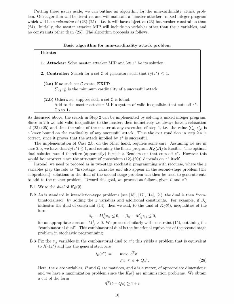
Putting these issues aside, we can outline an algorithm for the min-cardinality attack prob-lem. Our algorithm will be iterative, and will maintain a “master attacker” mixed-integer programwhich will be a relaxation of (23)-(25) – i.e. it will have objective (23) but weaker constraints than(24). Initially, the master attacker MIP will include no variables other than the z variables, andno constraints other than (25). The algorithm proceeds as follows.

Basic algorithm for min-cardinality attack problem

Iterate:

1. Attacker: Solve master attacker MIP and let z∗ be its solution.

2. Controller: Search for a set C of generators such that tC(z∗) ≤ 1.

(2.a) If no such set C exists, EXIT:∑ij z

∗ij is the minimum cardinality of a successful attack.

(2.b) Otherwise, suppose such a set C is found.Add to the master attacker MIP a system of valid inequalities that cuts off z∗.Go to 1.

As discussed above, the search in Step 2 can be implemented by solving a mixed integer program.Since in 2.b we add valid inequalities to the master, then inductively we always have a relaxationof (23)-(25) and thus the value of the master at any execution of step 1, i.e. the value

∑ij z

∗ij, is

a lower bound on the cardinality of any successful attack. Thus the exit condition in step 2.a iscorrect, since it proves that the attack implied by z∗ is successful.

The implementation of Case 2.b, on the other hand, requires some care. Assuming we are incase 2.b, we have that tC(z∗) ≤ 1, and certainly the linear program KC(A) is feasible. The optimaldual solution would therefore (apparently) furnish a Benders cut that cuts off z∗. However thiswould be incorrect since the structure of constraints (12)-(20)) depends on z∗ itself.

Instead, we need to proceed as in two-stage stochastic programming with recourse, where the zvariables play the role as “first-stage” variables and also appear in the second-stage problem (thesubproblem); solutions to the dual of the second-stage problem can then be used to generate cutsto add to the master problem. Toward this goal, we proceed as follows, given C and z∗:

B.1 Write the dual of KC(∅).B.2 As is standard in interdiction-type problems (see [18], [17], [14], [2]), the dual is then “com-

binatorialized” by adding the z variables and additional constraints. For example, if βij

indicates the dual of constraint (14), then we add, to the dual of KC(∅), inequalities of theform

βij −M1ijzij ≤ 0, −βij −M1

ijzij ≤ 0,

for an appropriate constant M 1ij > 0. We proceed similarly with constraint (15), obtaining the

“combinatorial dual”. This combinatorial dual is the functional equivalent of the second-stageproblem in stochastic programming.

B.3 Fix the zij variables in the combinatorial dual to z∗; this yields a problem that is equivalentto KC(z∗) and has the general structure

tC(z∗) = max cT v

Pv ≤ b + Qz∗. (26)

Here, the v are variables, P and Q are matrices, and b is a vector, of appropriate dimensions;and we have a maximization problem since the KC() are minimization problems. We obtaina cut of the form

αT (b+Qz) ≥ 1 + ε

10

where ε > 0 is a small constant and α is the vector of optimal dual variables to (26). Sinceby assumption tC(z∗) ≤ 1 this inequality cuts off z∗.

Note the use of the tolerance ε. The use of this parameter gives more power to the controller, i.e.“borderline” attacks are not considered successful. In a strict sense, therefore, we are not solvingthe optimization problem to exact precision; nevertheless in practice we expect our relaxation tohave negligible impact so long as ε is small. A deeper issue here is how to interpret truly borderlineattacks that are successful according to our strict model (and which our use of ε disallows); weexpect that in practice such attacks would be ambiguous and that the approximations incurredin modeling power flows, estimating demands levels, and so on, not to mention the numericalsensitivity of the integer and linear solvers being used, would have a far more significant impact onprecision.

2.1.1 Discussion

In order to make the outline provided in B.1-B.3 into a formal algorithm, we need to specify theconstants M 1

ij . As is well-known, the folklore of integer programming dictates that the M 1ij should

be chosen small to improve the quality of the linear programming relaxation of the master problem.

While this is certainly true, we have found that popular optimization packages show significantnumerical instability when solving power flow linear programs. In fact, in our experience it isprimarily this behavior that mandates that the M 1

ij should be kept as small as possible. In partic-ular we do not want the M 1

ij to grow with network since this would lead to an nonscalable approach.

It turns out that our formulation KC(A) is not ideal toward this goal. A particularly thornyissue is that the attack A may disconnect the network, and proving “reasonable” upper boundson the dual variables to (for example) constraint (13), when the network is disconnected, does notseem possible. In the next section we describe a different formulation for the min-cardinality attackproblem which is much better in this regard. Our eventual algorithm will apply steps B.1 - B.3 tothis improved formulation, while the rest of our basic algorithmic methodology as described abovewill remain unchanged.

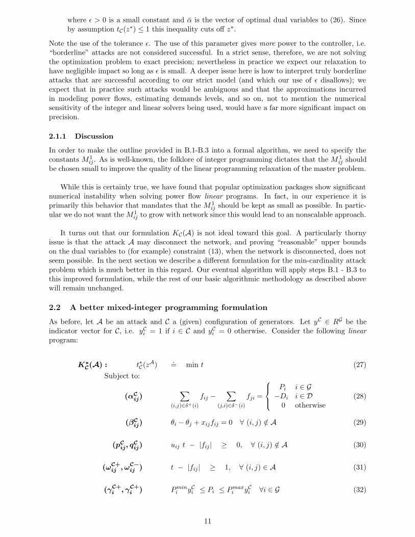
2.2 A better mixed-integer programming formulation

As before, let A be an attack and C a (given) configuration of generators. Let yC ∈ RG be theindicator vector for C, i.e. yCi = 1 if i ∈ C and yCi = 0 otherwise. Consider the following linearprogram:

K∗

C(A) : t∗C(z

A).= min t (27)

Subject to:

(αC

ij)∑

(i,j)∈δ+(i)

fij −∑

(j,i)∈δ−(i)

fji =

Pi i ∈ G−Di i ∈ D

0 otherwise(28)

(βC

ij) θi − θj + xijfij = 0 ∀ (i, j) /∈ A (29)

(pC

ij, qC

ij) uij t − |fij| ≥ 0, ∀ (i, j) /∈ A (30)

(ωC+

ij , ωC−

ij ) t − |fij| ≥ 1, ∀ (i, j) ∈ A (31)

(γC+

i , γC+

i ) Pmini yCi ≤ Pi ≤ Pmax

i yCi ∀i ∈ G (32)

11

(µC)∑

j∈DDj ≥ Tmin

∑

j∈DDnom

j

, (33)

(∆C

j ) Dj ≤ Dnomj ∀j ∈ D (34)

P ≥ 0, D ≥ 0. (35)

To the left of each constraint we have indicated the corresponding dual variable – (30) is really twoconstraints written as one, and the same with (31).

Note that we do not force fij = 0 for (i, j) ∈ A. Moreover arcs (i, j) ∈ A are also exemptedfrom constraint (29). Thus, the controller has significantly more power than in KC(A). However,because of constraint (31), we have t∗C(z

A) > 1 as soon as any of the arcs in A actually carries flow.We can summarize these remarks as follows:

Remark 2.4 A defeats C if and only if t∗C(zA) > 1.

Note that the above formulation depends on C only through constraint (32). Using appropriatematrices Af , Aθ, AP , AD, At, and vector b, the formulation can be abbreviated as

K∗

C(A) : t∗C(z

A).= min t

Subject to:

Aff + Aθθ + APP + ADD + Att ≥ b

Pmini yCi ≤ Pi ≤ Pmax

i yCi , ∀i ∈ G

Allowing the y quantities to become 0/1 variables, we obtain the problem

t∗(zA).= min t (36)

Subject to:

Aff + Aθθ + APP + ADD + Att ≥ b (37)

Pmini yi ≤ Pi ≤ Pmax

i yi, ∀i ∈ G (38)

yi = 0 or 1, ∀i ∈ G. (39)

This is the controller’s problem: we have that t∗(zA) ≤ 1 if and only if there exists some configu-ration of the generators that defeats A.

However, for the purposes of this section, we will assume C is given and that the yC are constants.We can now write the dual of K∗

C(A), suppressing the index C from the variables, for clarity.

AC(A) : max∑

i∈cG

yCi Pmini γ−i −

∑

i∈GyCi P

maxi γ+

i −∑

j∈DDnom

j ∆j +∑

j∈DDnom

j µj +∑

(i,j)∈E

ωij

Subject to:

(fij) αi − αj + xijβij − pij + qij + ω+ij − ω−

ij = 0 ∀(i, j) ∈ E (40)

(θi)∑

(i,j)∈δ+(i)

βij −∑

(j,i)∈δ−(i)

βji = 0 ∀i ∈ V (41)

(t)∑

(i,j)∈E

uij(pij + qij) +∑

(i,j)∈E

(ω+ij + ω−

ij) ≤ 1 (42)

(Pi) −αi − γ−i + γ+i = 0 ∀i ∈ G (43)

(Dj) αj + µ−∆j ≤ 0 ∀j ∈ D (44)

(ξ+ij , ξ−ij) x

1/2ij |βij | ≤ M(1− zAij ) ∀(i, j) ∈ E (45)

12

(%ij) pij + qij ≤1

uij(1− zAij ) ∀(i, j) ∈ E (46)

(ηij) ω+ij + ω−

ij ≤ zAij ∀(i, j) ∈ E (47)

ω+ij ≥ 0, ω−

ij ≥ 0, pij ≥ 0, qij ≥ 0 ∀(i, j) ∈ Eγ+

i , γ−i ≥ 0 ∀i ∈ G

∆j ≥ 0 ∀j ∈ Dµ ≥ 0

δij , βij free ∀(i, j) ∈ Eαi free ∀i ∈ V.

As before, for each constraint we indicate the corresponding dual variable. In (45), M is anappropriately chosen constant (we will provide a precise value for it below). Note that we are

scaling βij by x1/2ij – this is allowable since x

1/2ij > 0; the reason for this scaling will become clear

below.Abbreviating

(αC , βC , pC , qC , ωC+, ωC−, γC−, γC+, µC ,∆C) = ψC ,

we have that AC(A) can be rewritten as:

max{wTC ψ

C : AψC ≤ b + B(1− zA

)}(48)

where A, B, wC and b are appropriate matrices and vectors. Consequently, we can now rewrite themin-cardinality attack problem:

min∑

(i,j)

zij (49)

Subject to: tC ≥ 1 + ε, ∀ C ⊆ G (50)

wTC ψ

C − tC ≥ 0, ∀ C ⊆ G, (51)

AψC + Bz ≤ b + B ∀ C ⊆ G, (52)

zij = 0 or 1, ∀ (i, j). (53)

This formulation, of course, is exponentially large. An alternative is to use Benders cuts – havingsolved the linear program AC(A), let (f , θ, t, P , D, ξ+, ξ−, %, η) be optimal dual variables. Then theresulting Benders cut is

tC +∑

(i,j)∈E

((ξ+ij + ξ−ij)M(1 − zij)) +∑

(i,j)∈E

(1

uij%ij(1− zij)) +

∑

(i,j)∈E

ηijzij ≥ 1 + ε, (54)

We can now update our algorithmic template for the min-cardinality problem.

Updated algorithm for min-cardinality attack problem

Iterate:

1. Attacker: Solve master attacker MIP, obtaining attack A.

2. Controller: Solve the controller’s problem (36)-(39) to search for a setC of generators such that t∗C(z

A) ≤ 1.

(2.a) If no such set C exists, EXIT:A is a minimum cardinality successful attack.

(2.b) Otherwise, suppose such a set C is found. Then(2.b.1) Add to the master the Benders’ cut (54), and, optionally(2.b.2) Add to the master the entire system (50)-(52),

Go to 1.

13

Clearly, option (2.b.2) can only be exercised sparingly (if ever). Below we will discuss how wechoose, in our implementation, between (2.b.1) and (2.b.2). We will also describe how to (signif-icantly) strengthen the straightforward Benders cut (54). One point to note is that the cuts (orsystems) arising from different configurations C reinforce one another.

At each iteration of the algorithm, the master attacker MIP becomes a stronger relaxation for themin-cardinality problem, and thus its solution in step 1 provides a lower bound for the problem.Thus, if in a certain execution of step 2 we certify that t∗C(z

A) > 1 for every configuration C, wehave solved the min-cardinality problem to optimality.

What we have above is a complete outline of our algorithm. In order to make the algorithmeffective we need to further sharpen the approach. In particular, we need set the constant M toas small a value as possible, and we need to develop stronger inequalities than the basic Benders’cuts.

2.2.1 Setting M

In this section we show how to set for M a value that does not grow with network size.

Lemma 2.5 We can set

M = max(i,j)∈E

{1

√xij uij

.

}(55)

Proof. Given an attack A, consider a connected component K of N − A. For any arc (i, j) withboth ends in K, ω+

ij + ω−ij = 0 by (47). Hence we can rewrite constraints (40)-(41) over all arcs

with both ends in K as follows:

NTKαK + XKβK = pK − qK , (56)

NKβK = 0. (57)

Here, NK is the node arc incidence matrix of K, αK , βK , pK , qK are the restrictions of α, β, p, q toK, and XK is the diagonal matrix diag{xij : (i, j) ∈ K}. From this system we obtain

NKX−1K NKαK = NKX

−1K (pK − qK). (58)

The matrix NKX−1K NK has one-dimensional null space and thus we have one degree of freedom in

choosing αK . Thus, to solve (58), we can remove from NK an arbitrary row, obtaining NK , andremove the same row from αK , obtaining αK . Thus, (58) is equivalent to:

NKX−1K NKαK = NKX

−1K (pK − qK), (59)

The matrix NKX−1K NK and thus (59) has a unique solution (given pK − qK); we complete this to

a solution to (58) by setting to zero the entry of αK that was removed. Moreover,

X−1/2K NT

KαK = X−1/2K NT

KαK = X−1/2K NT

K(NKX−1K NT

K)−1NKX−1K (pK − qK). (60)

The matrixM = X

−1/2K NT

K (NKX−1K NT

K)−1 NKX−1/2K

is symmetric and idempotent, e.g. MM T = I. Thus, from (60) we get

‖X−1/2K NT

KαK‖2 ≤ ‖M‖2 ‖X−1/2K (pK − qK)‖2 ≤ ‖X−1/2

K (pK − qK)‖2, (61)

14

where the last inequality follows from the idempotent attribute. Because of constraints (42), (46)and (47), we can see that the right-hand side of (61) is upper-bounded by the value of the convexmaximization problem,

max∑

(i,j)∈E

x−1ij (pij − qij)2 (62)

s.t.∑

(i,j)∈E

uij(pij + qij) ≤ 1 (63)

pij ≥ 0, qij ≥ 0, (64)

which, as is easily seen, equals

max(i,j)∈E

{1

xiju2ij

}.

2.2.2 Tightening the formulation

In this Section we describe a family of inequalities that are valid for the attacker problem. Thesecuts seek to capture the interplay between the flow conservation equations and Ohm’s law. Firstwe present a technical result.

Lemma 2.6 Let Q be matrix with r rows with rank r, and let A = QT (QQT )−1Q ∈ Rr×r. LetB := I −A. Then for any p ∈ Rr we have

‖p‖22 = ‖Ap‖22 + ‖Bp‖22 (65)

‖p‖1 ≥ |(Ap)j |+ |(Bp)j| ∀j = 1 . . . r (66)

Proof. A and B are symmetric and idempotent, i.e., A2 = A, B2 = B, and any p ∈ Rr can bewritten as p = Ap + Bp. Multiplying equation this by p and using the fact that A and B aresymmetric and idempotent we get (65):

pT p = pTAp+ pTBp (67)

= pTA2p+ pTB2p (68)

‖p‖22 = ‖Ap‖22 + ‖Bp‖22 (69)

We also have ATB = A(I −A) = A−A2 = 0, so yTATBy = 0 for any y ∈ Rr. Thus, if we renameAp = x and Bp = y, then the following holds: p = x+ y, xT y = 0, ‖p‖22 = ‖x‖22 + ‖y‖22.

Let 1 ≤ j ≤ r. We have

‖p‖22 − (|xj |+ |yj |)2 = ‖x‖22 + ‖y‖22 − (|xj |+ |yj|)2 =∑

i,i6=j

x2i +

∑

i,i6=j

y2i − 2|xjyj|

where the first equality follows from (65). Since xT y = 0, we have |xjyj| = |∑

i,i6=j xiyi|. Hence,

∑

i,i6=j

x2i +

∑

i,i6=j

y2i − 2|xjyj| =

∑

i,i6=j

x2i +

∑

i,i6=j

y2i − 2

∣∣∣∣∣∣

∑

i,i6=j

xiyi

∣∣∣∣∣∣(70)

≥∑

i,i6=j

x2i +

∑

i,i6=j

y2i − 2

∑

i,i6=j

|xiyi| (71)

=∑

i,i6=j

(|xi| − |yi|)2 (72)

≥ 0 (73)

So we have ‖p‖22 − (|xj |+ |yj |)2 ≥ 0, which implies ‖p‖1 ≥ ‖p‖2 ≥ (|xj |+ |yj|) ∀j = 1 . . . r.

As a consequence of this result we now have:

15

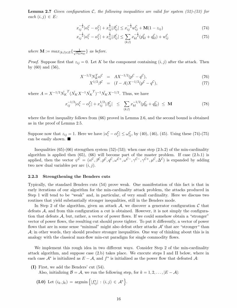
Lemma 2.7 Given configuration C, the following inequalities are valid for system (52)-(53) foreach (i, j) ∈ E:

x− 1

2

ij |αCi − αC

j |+ x1

2

ij|βCij | ≤ x− 1

2

ij wCij + M(1− zij) (74)

x− 1

2

ij |αCi − αC

j |+ x1

2

ij|βCij | ≤∑

(k,l)

x− 1

2

kl (pCkl + qCkl) + wCij (75)

where M := max(k,l)∈E{ 1√xklukl

} as before.

Proof. Suppose first that zij = 0. Let K be the component containing (i, j) after the attack. Thenby (60) and (56),

X−1/2NTKα

C = AX−1/2(pC − qC), (76)

X1/2βC = (I −A)X−1/2(pC − qC), (77)

where A = X−1/2NKT(NKX

−1NKT)−1NKX

−1/2. Thus, we have

x−1/2ij |αC

i − αCj |+ x

1/2ij |βCij | ≤

∑

(k,l)

x−1/2kl (pCkl + qCkl) ≤ M (78)

where the first inequality follows from (66) proved in Lemma 2.6, and the second bound is obtainedas in the proof of Lemma 2.5.

Suppose now that zij = 1. Here we have |αCi −αC

j | ≤ ωCij, by (40), (46), (45). Using these (74)-(75)

can be easily shown.

Inequalities (65)-(66) strengthen system (52)-(53); when case step (2.b.2) of the min-cardinalityalgorithm is applied then (65), (66) will become part of the master problem. If case (2.b.1) isapplied, then the vector ψC = (αC , βC , pC , qC , ωC+, ωC−, γC−, γC+, µC ,∆C) is expanded by addingtwo new dual variables per arc (i, j).

2.2.3 Strengthening the Benders cuts

Typically, the standard Benders cuts (54) prove weak. One manifestation of this fact is that inearly iterations of our algorithm for the min-cardinality attack problem, the attacks produced inStep 1 will tend to be “weak” and, in particular, of very small cardinality. Here we discuss tworoutines that yield substantially stronger inequalities, still in the Benders mode.

In Step 2 of the algorithm, given an attack A, we discover a generator configuration C thatdefeats A, and from this configuration a cut is obtained. However, it is not simply the configura-tion that defeats A, but, rather, a vector of power flows. If we could somehow obtain a “stronger”vector of power flows, the resulting cut should prove tighter. To put it differently, a vector of powerflows that are in some sense “minimal” might also defeat other attacks A′ that are “stronger“ thanA; in other words, they should produce stronger inequalities. One way of thinking about this is inanalogy with the classical max-flow min-cut paradigm for single commodity flows.

We implement this rough idea in two different ways. Consider Step 2 of the min-cardinalityattack algorithm, and suppose case (2.b) takes place. We execute steps I and II below, where ineach case A∗ is initialized as E −A, and f ∗ is initialized as the power flow that defeated A:

(I) First, we add the Benders’ cut (54).Also, initializing B = A, we run the following step, for k = 1, 2, . . . , |E −A|:

(I.0) Let (ik, jk) = argmin{|f∗ij | : (i, j) ∈ A∗

}.

16

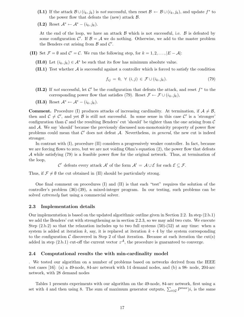
(I.1) If the attack B ∪ (ik, jk) is not successful, then reset B ← B ∪ (ik, jk), and update f ∗ tothe power flow that defeats the (new) attack B.

(I.2) Reset A∗ ← A∗ − (ik, jk).

At the end of the loop, we have an attack B which is not successful, i.e. B is defeated bysome configuration C ′. If B = A we do nothing. Otherwise, we add to the master problemthe Benders cut arising from B and C ′.

(II) Set F = ∅ and C ′ = C. We run the following step, for k = 1, 2, . . . , |E −A|:

(II.0) Let (ik, jk) ∈ A∗ be such that its flow has minimum absolute value.

(II.1) Test whether A is successful against a controller which is forced to satisfy the condition

fij = 0, ∀ (i, j) ∈ F ∪ (ik, jk). (79)

(II.2) If not successful, let C ′ be the configuration that defeats the attack, and reset f ∗ to thecorresponding power flow that satisfies (79). Reset F ← F ∪ (ik, jk),

(II.3) Reset A∗ ← A∗ − (ik, jk).

Comment. Procedure (I) produces attacks of increasing cardinality. At termination, if A 6= B,then and C 6= C ′, and yet B is still not successful. In some sense in this case C ′ is a ’stronger’configuration than C and the resulting Benders’ cut ’should’ be tighter than the one arising from Cand A. We say ’should’ because the previously discussed non-monotonicity property of power flowproblems could mean that C ′ does not defeat A. Nevertheless, in general, the new cut is indeedstronger.

In contrast with (I), procedure (II) considers a progressively weaker controller. In fact, becausewe are forcing flows to zero, but we are not voiding Ohm’s equation (2), the power flow that defeatsA while satisfying (79) is a feasible power flow for the original network. Thus, at termination ofthe loop,

C′ defeats every attack A′ of the form A′ = A∪ E for each E ⊆ F .Thus, if F 6= ∅ the cut obtained in (II) should be particularly strong.

One final comment on procedures (I) and (II) is that each “test” requires the solution of thecontroller’s problem (36)-(39), a mixed-integer program. In our testing, such problems can besolved extremely fast using a commercial solver.

2.3 Implementation details

Our implementation is based on the updated algorithmic outline given in Section 2.2. In step (2.b.1)we add the Benders’ cut with strengthening as in section 2.2.3, so we may add two cuts. We executeStep (2.b.2) so that the relaxation includes up to two full systems (50)-(52) at any time: when asystem is added at iteration k, say, it is replaced at iteration k + 4 by the system correspondingto the configuration C discovered in Step 2 of that iteration. Because at each iteration the cut(s)added in step (2.b.1) cut-off the current vector zA, the procedure is guaranteed to converge.

2.4 Computational results the with min-cardinality model

. We tested our algorithm on a number of problems based on networks derived from the IEEEtest cases [16]: (a) a 49-node, 84-arc network with 14 demand nodes, and (b) a 98- node, 204-arcnetwork, with 28 demand nodes

Tables 1 presents experiments with our algorithm on the 49-node, 84-arc network, first using aset with 4 and then using 8. The sum of maximum generator outputs,

∑i∈G P

max)i, is the same

17

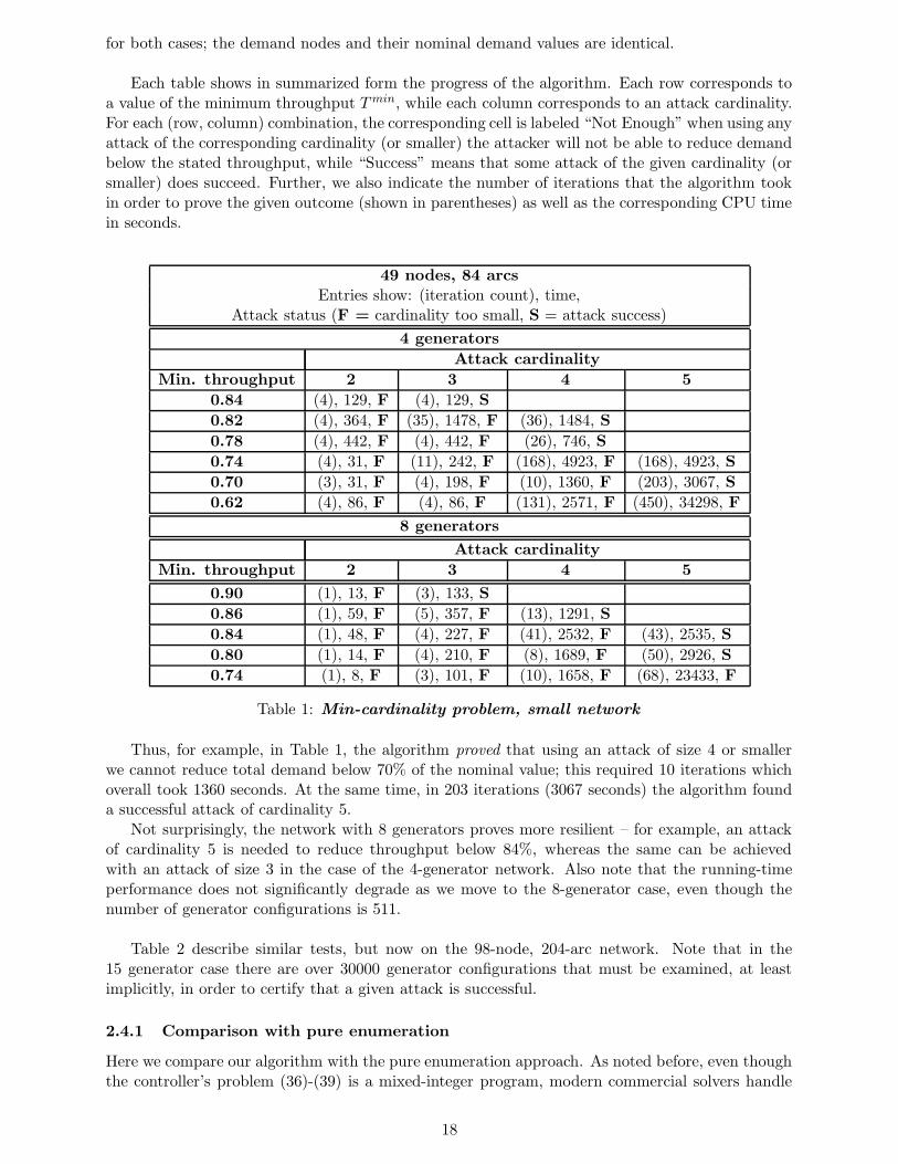
for both cases; the demand nodes and their nominal demand values are identical.

Each table shows in summarized form the progress of the algorithm. Each row corresponds toa value of the minimum throughput Tmin, while each column corresponds to an attack cardinality.For each (row, column) combination, the corresponding cell is labeled “Not Enough” when using anyattack of the corresponding cardinality (or smaller) the attacker will not be able to reduce demandbelow the stated throughput, while “Success” means that some attack of the given cardinality (orsmaller) does succeed. Further, we also indicate the number of iterations that the algorithm tookin order to prove the given outcome (shown in parentheses) as well as the corresponding CPU timein seconds.

49 nodes, 84 arcsEntries show: (iteration count), time,

Attack status (F = cardinality too small, S = attack success)

4 generators

Attack cardinality

Min. throughput 2 3 4 5

0.84 (4), 129, F (4), 129, S

0.82 (4), 364, F (35), 1478, F (36), 1484, S

0.78 (4), 442, F (4), 442, F (26), 746, S

0.74 (4), 31, F (11), 242, F (168), 4923, F (168), 4923, S

0.70 (3), 31, F (4), 198, F (10), 1360, F (203), 3067, S

0.62 (4), 86, F (4), 86, F (131), 2571, F (450), 34298, F

8 generators

Attack cardinality

Min. throughput 2 3 4 5

0.90 (1), 13, F (3), 133, S

0.86 (1), 59, F (5), 357, F (13), 1291, S

0.84 (1), 48, F (4), 227, F (41), 2532, F (43), 2535, S

0.80 (1), 14, F (4), 210, F (8), 1689, F (50), 2926, S

0.74 (1), 8, F (3), 101, F (10), 1658, F (68), 23433, F

Table 1: Min-cardinality problem, small network

Thus, for example, in Table 1, the algorithm proved that using an attack of size 4 or smallerwe cannot reduce total demand below 70% of the nominal value; this required 10 iterations whichoverall took 1360 seconds. At the same time, in 203 iterations (3067 seconds) the algorithm founda successful attack of cardinality 5.

Not surprisingly, the network with 8 generators proves more resilient – for example, an attackof cardinality 5 is needed to reduce throughput below 84%, whereas the same can be achievedwith an attack of size 3 in the case of the 4-generator network. Also note that the running-timeperformance does not significantly degrade as we move to the 8-generator case, even though thenumber of generator configurations is 511.

Table 2 describe similar tests, but now on the 98-node, 204-arc network. Note that in the15 generator case there are over 30000 generator configurations that must be examined, at leastimplicitly, in order to certify that a given attack is successful.

2.4.1 Comparison with pure enumeration

Here we compare our algorithm with the pure enumeration approach. As noted before, even thoughthe controller’s problem (36)-(39) is a mixed-integer program, modern commercial solvers handle

18

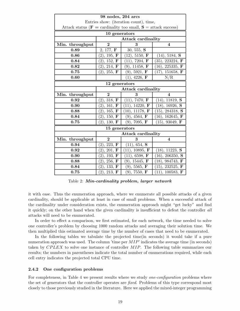
98 nodes, 204 arcsEntries show: (iteration count), time,

Attack status (F = cardinality too small, S = attack success)

10 generators

Attack cardinality

Min. throughput 2 3 4

0.89 2, 177, F 30, 555, S

0.86 (2), 195, F (12), 5150, F (14), 5184, S

0.84 (2), 152, F (11), 7204, F (35), 223224, F

0.82 (2), 214, F (9), 11458, F (16), 225335, F

0.75 (2), 255, F (9), 5921, F (17), 151658, F

0.60 (1), 4226, F N/R

12 generators

Attack cardinality

Min. throughput 2 3 4

0.92 (2), 318, F (11), 7470, F (14), 11819, S

0.90 (2), 161, F (11), 14220, F (18), 16926, S

0.88 (2), 165, F (10), 11178, F (15), 284318, S

0.84 (2), 150, F (9), 4564, F (16), 162645, F

0.75 (2), 130, F (9), 7095, F (15), 93049, F

15 generators

Attack cardinality

Min. throughput 2 3 4

0.94 (2), 223, F (11), 654, S

0.92 (2), 201, F (11), 10895, F (18), 11223, S

0.90 (2), 193, F (11), 6598, F (16), 206350, S

0.88 (2), 256, F (9), 15445, F (18), 984743, F

0.84 (2), 133, F (9), 5565, F (15), 232525, F

0.75 (2), 213, F (9), 7550, F (11), 100583, F

Table 2: Min-cardinality problem, larger network

it with ease. Thus the enumeration approach, where we enumerate all possible attacks of a givencardinality, should be applicable at least in case of small problems. When a successful attack ofthe cardinality under consideration exists, the enumeration approach might “get lucky” and findit quickly; on the other hand when the given cardinality is insufficient to defeat the controller allattacks will need to be enumerated.

In order to effect a comparison, we first estimated, for each network, the time needed to solveone controller’s problem by choosing 1000 random attacks and averaging their solution time. Wethen multiplied this estimated average time by the number of cases that need to be enumerated.

In the following tables we tabulate the projected time(in seconds) it would take if a purenumeration approach was used. The column ’time perMIP ’ indicates the average time (in seconds)taken by CPLEX to solve one instance of controller MIP . The following table summarizes ourresults; the numbers in parentheses indicate the total number of enumerations required, while eachcell entry indicates the projected total CPU time.

2.4.2 One configuration problems

For completeness, in Table 4 we present results where we study one-configuration problems wherethe set of generators that the controller operates are fixed. Problems of this type correspond mostclosely to those previously studied in the literature. Here we applied the mixed-integer programming

19

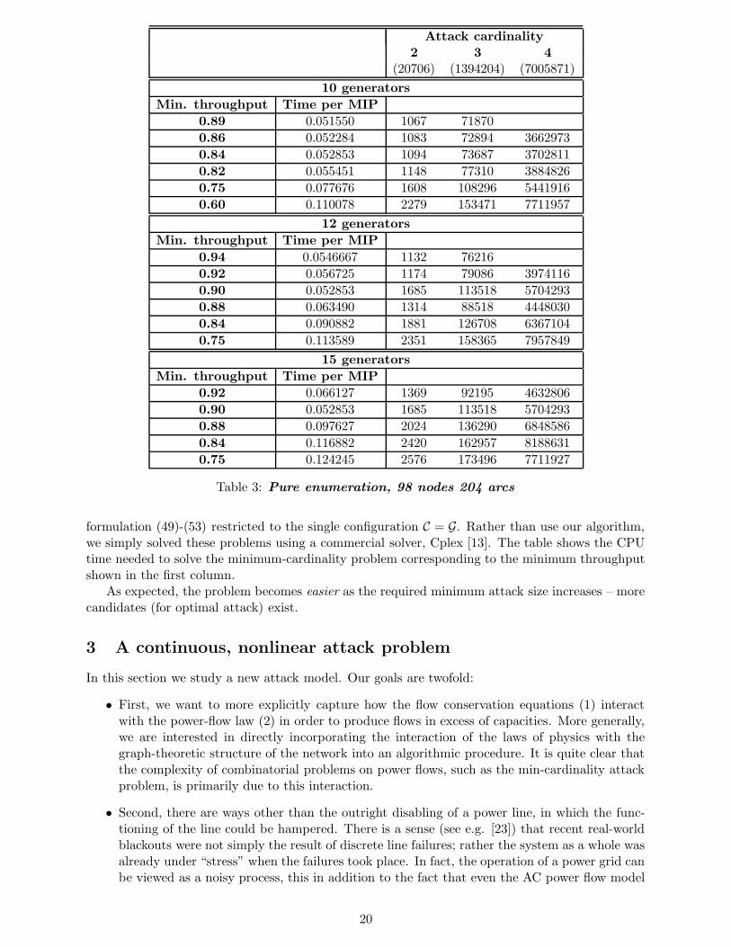
Attack cardinality2 3 4

(20706) (1394204) (7005871)

10 generators

Min. throughput Time per MIP

0.89 0.051550 1067 71870

0.86 0.052284 1083 72894 3662973

0.84 0.052853 1094 73687 3702811

0.82 0.055451 1148 77310 3884826

0.75 0.077676 1608 108296 5441916

0.60 0.110078 2279 153471 7711957

12 generators

Min. throughput Time per MIP

0.94 0.0546667 1132 76216

0.92 0.056725 1174 79086 3974116

0.90 0.052853 1685 113518 5704293

0.88 0.063490 1314 88518 4448030

0.84 0.090882 1881 126708 6367104

0.75 0.113589 2351 158365 7957849

15 generators

Min. throughput Time per MIP

0.92 0.066127 1369 92195 4632806

0.90 0.052853 1685 113518 5704293

0.88 0.097627 2024 136290 6848586

0.84 0.116882 2420 162957 8188631

0.75 0.124245 2576 173496 7711927

Table 3: Pure enumeration, 98 nodes 204 arcs

formulation (49)-(53) restricted to the single configuration C = G. Rather than use our algorithm,we simply solved these problems using a commercial solver, Cplex [13]. The table shows the CPUtime needed to solve the minimum-cardinality problem corresponding to the minimum throughputshown in the first column.

As expected, the problem becomes easier as the required minimum attack size increases – morecandidates (for optimal attack) exist.

3 A continuous, nonlinear attack problem

In this section we study a new attack model. Our goals are twofold:

• First, we want to more explicitly capture how the flow conservation equations (1) interactwith the power-flow law (2) in order to produce flows in excess of capacities. More generally,we are interested in directly incorporating the interaction of the laws of physics with thegraph-theoretic structure of the network into an algorithmic procedure. It is quite clear thatthe complexity of combinatorial problems on power flows, such as the min-cardinality attackproblem, is primarily due to this interaction.

• Second, there are ways other than the outright disabling of a power line, in which the func-tioning of the line could be hampered. There is a sense (see e.g. [23]) that recent real-worldblackouts were not simply the result of discrete line failures; rather the system as a whole wasalready under “stress” when the failures took place. In fact, the operation of a power grid canbe viewed as a noisy process, this in addition to the fact that even the AC power flow model

20

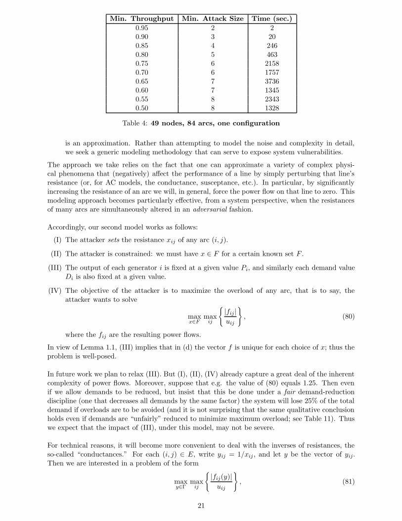
Min. Throughput Min. Attack Size Time (sec.)

0.95 2 20.90 3 200.85 4 2460.80 5 4630.75 6 21580.70 6 17570.65 7 37360.60 7 13450.55 8 23430.50 8 1328

Table 4: 49 nodes, 84 arcs, one configuration

is an approximation. Rather than attempting to model the noise and complexity in detail,we seek a generic modeling methodology that can serve to expose system vulnerabilities.

The approach we take relies on the fact that one can approximate a variety of complex physi-cal phenomena that (negatively) affect the performance of a line by simply perturbing that line’sresistance (or, for AC models, the conductance, susceptance, etc.). In particular, by significantlyincreasing the resistance of an arc we will, in general, force the power flow on that line to zero. Thismodeling approach becomes particularly effective, from a system perspective, when the resistancesof many arcs are simultaneously altered in an adversarial fashion.

Accordingly, our second model works as follows:

(I) The attacker sets the resistance xij of any arc (i, j).

(II) The attacker is constrained: we must have x ∈ F for a certain known set F .

(III) The output of each generator i is fixed at a given value Pi, and similarly each demand valueDi is also fixed at a given value.

(IV) The objective of the attacker is to maximize the overload of any arc, that is to say, theattacker wants to solve

maxx∈F

maxij

{|fij|uij

}, (80)

where the fij are the resulting power flows.

In view of Lemma 1.1, (III) implies that in (d) the vector f is unique for each choice of x; thus theproblem is well-posed.

In future work we plan to relax (III). But (I), (II), (IV) already capture a great deal of the inherentcomplexity of power flows. Moreover, suppose that e.g. the value of (80) equals 1.25. Then evenif we allow demands to be reduced, but insist that this be done under a fair demand-reductiondiscipline (one that decreases all demands by the same factor) the system will lose 25% of the totaldemand if overloads are to be avoided (and it is not surprising that the same qualitative conclusionholds even if demands are “unfairly” reduced to minimize maximum overload; see Table 11). Thuswe expect that the impact of (III), under this model, may not be severe.

For technical reasons, it will become more convenient to deal with the inverses of resistances, theso-called “conductances.” For each (i, j) ∈ E, write yij = 1/xij , and let y be the vector of yij.Then we are interested in a problem of the form

maxy∈Γ

maxij

{|fij(y)|uij

}, (81)

21

where Γ is an appropriate set, and as just discussed the notation fij(y) is justified.

A relevant example of a set Γ is that given by:

∑

ij

1

yij≤ B,

1

xUij

≤ yij ≤1

xLij

∀ (i, j), (82)

where B is a given ’budget’, and, for any arc (i, j), xLij and xU

ij and indicates a minimum andmaximum value for the resistance at (i, j). Suppose the initial resistances xij are all equal to somecommon value x, and we set xL

ij = x for every (i, j), and B = k θ x + (|E| − k)x, where k > 0 is aninteger and θ > 1 is large. Then, roughly speaking, we are approximately allowing the adversary tomake the resistance of (up to) k arcs “very large”, while not decreasing any resistance, a problemclosely reminiscent of the classical N−K problem. We will make this statement more precise later.

If the objective in (81) is convex then the optimum will take place at some extreme point. Ingeneral, the objective is not convex; but computational experience shows that we tend to convergeto points that are either extreme points, or very close to extreme points (see the computationalsection).

3.1 Solution methodology

Problem (81) is not smooth. However, it is equivalent to:

maxy,p

∑

ij

fij(y)

uij(pij − qij) (83)

s.t.∑

ij

(pij + qij) = 1, (84)

y ∈ Γ, p, q ≥ 0. (85)

In order to work with this formulation we need to develop a more explicit representation of thefunctions fij(y). This will require a sequence of technical results given in the following section;however a brief discussion of our approach follows.

Problem (83), although smooth, is not concave. A relatively recent research thrust has focused onadapting techniques of (convex) nonlinear programming to nonconvex problems. This work hasresulted in a very large literature with interesting and useful results; see [15], [4]. Since one isattempting to solve non-convex minimization (and thus, NP-hard) problems, there is no guaranteethat a global optimum will be found by these techniques. One can sometimes assume that a globaloptimum is approximately known; and the techniques then are likely to converge to the optimumfrom an appropriate guess.

In any case, (a) the use of nonlinear models allows for much richer representation of problems,(b) the very successful numerical methodology backing convex optimization is brought to bear,and (c) even though only a local optimum may be found, at least one is relying on an agnostic,“honest” optimization technique as opposed to a pure heuristic or a method that makes structuralassumptions about the nature of the optimum in order to simplify the problem.

In our approach we will indeed rely on this methodology – items (a)-(c) precisely capture thereasons for our choice. Points (a) and (c) are particularly important in our blackout context: weare very keen on modeling the nonlinearities, and on using a truly agnostic algorithm to root outhidden weaknesses in a network. And from a computational perspective, the approach does payoff, because we are able to comfortably handle problems with on the order of 1000 arcs.

As a final point, note that in principle one could rely on a branch-and-bound procedure toactually find the global optimum. This will be a subject for future research.

22

3.1.1 Laplacians

In this section we present some background material on linear algebra and Laplacians of graphs –the results are standard but we include a proof for completeness and continuity. See [7] for relevantmaterial.

As before we have a directed network G with n nodes and m arcs and with node-arc incidencematrix N . As before we assume G is connected. For a positive diagonal matrix Y ∈ Rm×m we willwrite

L = NYNT , J = L +1

n11T . (86)

where 1 ∈ Rn is the vector (1, 1, . . . , 1)T . L is called a generalized Laplacian. We have that L issymmetric positive-semidefinite. If λ1 ≤ λ2 ≤ . . . ≤ λn are the eigenvalues of L, and v1, v2, . . . , vn

are the corresponding unit-norm eigenvectors, then

λ1 = 0, but λi > 0 for i > 1, (87)

because G is connected, and thus L has rank n− 1. The same argument shows that since N1 = 0,we can assume v1 = n−1/2 1. Finally, since different eigenvectors are are orthogonal, we have1T vi = 0 for 2 ≤ i ≤ n.

Lemma 3.1 L and J have the same eigenvectors, and all but one of their eigenvalues coincide.Further, J is invertible.

Proof. By (87),

Lv1 = 0, Jv1 =1

n11T v1 = v1, (88)

and further

Jvi = Lvi = λivi. (89)

Lemma 3.2 Let b ∈ Rn. Any solution to the system of equations Lα = b is of the form

α = J−1b+ δ1,

for some δ ∈ R.

Proof. We have that L =∑n

i=2 λivivTi , and, by Lemma 3.1, J−1 =

∑ni=2

1λiviv

Ti + 1

n11T . Now,the system of equations Lα = b is feasible if and only if b lies in the column space of matrix L andwhen it is so we can write b =

∑ni=2 vi(v

Ti b). Assuming that this is the case, defining

α.= J−1b =

n∑

i=2

1

λivi(v

Ti b) (90)

we will have Lα = b. Suppose that α is another vector satisfying Lα = b. Then L(α− α) = 0, andconsequently α = α+ δ1, for some δ.

DefineP = I − J.

Note that the eigenvalues of P are 0 and 1− λi, 2 ≤ i ≤ n; thus if we have

∑

(u,v)

yuv < 1/2, for all u, (91)

23

then it is not difficult to show that

0 < 1− λi < 1, for all i ≥ 2. (92)

(See [19] for related background). In such a case we can write

J−1 = (I − P )−1 = I + P + P 2 + P 3 + . . . , (93)

in other words, the series in (93) converges to J−1.

Lemma 3.3 For any integer k > 0, P k = (I −NYNT )k − 1n11T .

Proof. We will prove the statement by induction on k, while also proving that (I−NYN T )k11T =11T . The case k = 1 holds by definition. For the general inductive step, we have

P k+1 =

[(I −NYNT )k − 1

n11T

]P (94)

= (I −NYNT )k+1 − 1

n(I −NYNT )k11T − 1

n11T

[(I −NYNT )− 1

n11T

](95)

= (I −NYNT )k+1 − 1

n11T , (96)

because by induction

(I −NYNT )k11T = (I −NYNT )k−1(I −NYNT )11T = 11T , (97)

and

11T[(I −NYNT )− 1

n11T

]= 11T − 1

n11T 11T = 0. (98)

The second inductive statement is similarly proved.

3.2 Model details

We will now apply the above techniques to our problem (83)-(85), where, as per our modelingassumption (III), b denote the (fixed) net supply vector, i.e. bi = Pi for a generator i, bi = −Di fora demand node i, and bi = 0 otherwise. Denoting by Y the diagonal matrix with entries 1/yij , wehave that given Y the unique power flows f and voltages θ are obtained by solving the system

NT θ − Y −1f = 0

Nf = b.

Note that if we scale Y and b by a multiplicative factor µ > 0 then we obtain an equivalent system,e.g. the power flows f increase by a factor of µ and the angles θ do not change. Thus, assumingΓ ⊆ Rn

+ is bounded (as is the case if we use (82)) then as a first step to solving (83)-(85) we canscale Γ so that condition (91) holds for every y ∈ Γ. Consequently, by (92), we can assume thatthere is a constant r < 1 such that 1− λi < r for 2 ≤ i ≤ n. In what follows we will always makethis assumption.

By Lemma 3.2 each solution to (99)-(99) is of the form

θ = J−1b+ δ1 for some δ ∈ R, (99)

f = Y NTJ−1b. (100)

For each arc (i, j) denote by nij the column of N corresponding to (i, j), i.e., nij := Neij , whereeij ∈ Rm is the vector with a 1 at entry (i, j) and zero otherwise. Using (93) we therefore have

fij = yijnTij

[I + P + P 2 + P 3 + . . .

]b, ∀(i, j), and (101)

θi − θj = nTijθ = nT

ij

[I + P + P 2 + P 3 + . . .

]b = nT

ij

∞∑

k=0

P k b, (102)

24

In the following we will be handling expressions with infinite series such as the above. In order tofacilitate the analysis we need a ’uniform convergence’ argument, as follows. Given y ∈ Γ, notethat we can write

P = P (y) = U(y)Λ(y)U(y)T , (103)

where U(y) is a unitary matrix and Λ(y) is the diagonal matrix containing the eigenvalues of P (y).Hence, for any k ≥ 1 and any arc (i, j) (and dropping the dependence on yst for simplicity),

|nTijP

kb| = |nTijUΛkUT b| < νk, (104)

for some ν < 1, by (92). We will rely on this bound below.

As a first consequence of (104) we have the following result, showing that appropriate assumptionsthe continuous model we consider is related to the network vulnerability models in Section 2.

Lemma 3.4 Let S be a set of arcs whose removal does not disconnect G. Suppose we fix the val-ues yij = 1/xij for each arc (i, j) /∈ S, and we likewise set yst = ε for each arc (s, t) ∈ S. Let(f(y), θ(y)) denote the resulting power flow, and let (f , θ) the solution to the power flow problemon G− S.

Then

(a) limε→0 fst(y) = 0, for all (s, t) ∈ S,

(b) For any (u, v) /∈ S, limε→0 fuv(y) = fuv.

(c) For any (u, v), limε→0(θu(y)− θv(y)) = θu − θv.

Proof. (a) Let G = G − (s, t), let N be node-arc incidence matrix of G, Y the restriction of Y toE − (s, t), and P = I − N Y NT − 1

n11T .

For any integer k ≥ 1 we have by Lemma 3.3

limε→0

P k = limε→0

(I −NYNT )k − 1

n11T = (I − NY NT )k − 1

n11T = P k. (105)

Consequently, by (101), for any (s, t) ∈ S,

limε→0

fst = limε→0

[ystn

Tst

( ∞∑

k=0

P k

)b

]=

∞∑

k=0

[limε→0

yst

(nT

stPkb)]

= 0, (106)

where the exchange between summation and limit is valid because of (104). The proof of (b), (c)are similar.

Lemma 3.4 can be interpreted as describing a particular type of attack that is feasible for theadversary under our models. Our computational experiments show that the pattern assumed bythe Lemma is approximately correct: given an attack budget, the attacker tends to concentratemost of the attack on a small number of arcs (essentially, making their resistance very large), whileat the same time attacking a larger number of lines with a small portion of the budget.

In the following set of results we determine efficient closed-form expressions for the gradient andHessian of the objective in (81). As before, we denote by nij the column of the node-arc incidencematrix of the network corresponding to arc (i, j).

25

Lemma 3.5 For any integer k > 0, and any arc (i, j)

(a) 1TP k = 0,

(b)∂

∂yij

[P kb

]= P

∂

∂yij

[P k−1b

]− nijn

TijP

k−1b.

Proof. Note that 1TP = 1T (I − J) = 1T (I −NYNT − 1n11T ) = 0. Hence 1TP k = 0.

∂

∂yij

[P kb

]=

∂

∂yij

[PP k−1b

]

=∂

∂yij

I −

∑

(u,v)∈E

yuv nuvnTuv −

1

n11T

P k−1b

=∂

∂yij

[P k−1b

]− ∂

∂yij

∑

(u,v)∈E

yuv nuvnTuv

P k−1b

− ∂

∂yij

[1

n11TP k−1b

]

=∂

∂yij

[P k−1b

]− ∂

∂yij

∑

(u,v)∈E

yuv nuvnTuv

P k−1b

=∂

∂yij

[P k−1b

]−

∑

(u,v)∈E

∂

∂yij

[yuv nuvn

TuvP

k−1b]

=∂

∂yij

[P k−1b

]−

∑

(u,v)∈E

[∂yuv

∂yij

]nuvn

TuvP

k−1b−∑

(u,v)∈E

yuv∂

∂yij

[nuvn

TuvP

k−1b]

=∂

∂yij

[P k−1b

]− nijn

TijP

k−1b−∑

(u,v)∈E

yuv nuvnTuv

∂

∂yij

[P k−1b

]

=

I −

∑

(u,v)∈E

yuv nuvnTuv

∂

∂yij

[P k−1b

]− nijn

TijP

k−1b

=

[P +

1

n11T

]∂

∂yij

[P k−1b

]− nijn

TijP

k−1b

= P∂

∂yij

[P k−1b

]− nijn

TijP

k−1b+∂

∂yij

[1

n11TP k−1b

]

= P∂

∂yij

[P k−1b

]− nijn

TijP

k−1b.

where the third and the last equality follow from (a).

Using the above recursive formula we can write the following expressions:

∂

∂yij[Pb] = −nijn

Tijb

∂

∂yij[P 2b] = P

∂

∂yij[Pb]− nijn

TijPb

∂

∂yij[P 3b] = P 2 ∂

∂yij[Pb]− Pnijn

TijPb− nijn

TijP

2b

∂

∂yij[P 4b] = P 3 ∂

∂yij[Pb]− P 2nijn

TijPb− Pnijn

TijP

2b− nijnTijP

3b

...∂

∂yij[P kb] = P k−1 ∂

∂yij[Pb]− P k−2nijn

TijPb− P k−3nijn

TijP

2b− . . .− nijnTijP

k−1b

26

Consequently, defining

∇ij =∂

∂yij

[I + P + P 2 + . . .

]b, (107)

we have

∇ij =[I + P + P 2 + . . .

] ∂

∂yij[Pb] −

(I + P + P 2 + . . .

)nijn

Tij

(P + P 2 + P 3 + . . .

)b

= −[I + P + P 2 + . . .

]nijn

Tijb −

(I + P + P 2 + . . .

)nijn

Tij

(I + P + P 2 + . . .− I

)b

= −(I + P + P 2 + . . .

)nijn

Tij

(I + P + P 2 + . . .

)b

= −J−1 nijnTij θ, (108)

where the last equality follows from (99) and (93), and the fact that nTij1 = 0.

Using (101), the gradient of function fuv(y) with respect to the variables yij can be written as:

∂fuv

∂yij= yuv n

Tuv

∂

∂yij

[I + P + P 2 + P 3 + . . .

]b = yuv n

Tuv ∇ij , (i, j) 6= (u, v) (109)

∂fij

∂yij= nT

ij

[I + P + P 2 + P 3 + . . .

]b + yij n

Tij

∂

∂yij

[I + P + P 2 + P 3 + . . .

]b

= nTij∇ij + yijn

Tij∇ij . (110)

We similarly develop close-form expressions for the second order derivatives. For (u, v) 6= (i, j), (u, v) 6=(h, k), we have the following :

∂2fuv

∂yij∂yhk= yuvn

Tuv [ (I + P + P 2 + P 3 + . . .)nijn

Tij (I + P + P 2 + P 3 + . . .)nhkn

Thk

+(I + P + P 2 + P 3 + . . .)nhknThk (I + P + P 2 + P 3 + . . .)nijn

Tij θ

= −yuvnTuvJ

−1[nijn

Tij∇hk + nhkn

Thk∇ij

]. (111)

Similarly, the remaining terms are:

∂2fuv

∂y2uv

= 2nTuv∇uv − 2 yuvn

TuvJ

−1nuvnTuv∇uv, (112)

∂2fuv

∂yuv∂yij= nT

uv ∇ij − yuv nTuvJ

−1[nijn

Tij ∇i + nuvn

Tuv ∇ij

](113)

3.3 Implementation details

We use LOQO [22] to solve problem (83)-(85), using Γ ={y ≥ 0 :

∑ij

1yij≤ B

}with values of B

that we selected. LOQO is an infeasible primal-dual, interior-point method applied to a sequence ofquadratic approximations to the given problem. The procedure stops if at any iteration the primaland dual problems are feasible and with objective values that are close to each other, in which casea local optimal solution is found. For numerical reasons, LOQO additionally uses an upper boundon the overall number of iterations to perform.

At each iteration of the method applied by LOQO, it requires the Hessian and gradient of theobjective function and the constraints. The latter are easy to derive. Note that using (109), (110),(111)-(113) one can obtain compact, closed-form expressions for the Hessian and gradient of theobjective. This approach requires the computation of quantities nT

uvJ−1nij for each pair of arcs

(i, j), (u, v). At any given iteration, we compute and (appropriately) store these quantities (whichcan be done in O(n2 + nm) space).

27

In order to compute nTuvJ

−1nij, for given (i, j) and (u, v), we simply solve the sparse linear systemon variables κ, λ:

NTκ− Y −1λ = 0 (114)

Nλ = nij. (115)

As in (99), we have κ = J−1nij + δ1 for some real δ. But then nTuvκ = nT

uvJ−1nij, the desired

quantity. In order to solve (114)-(115) we use Cplex (to solve a nominal linear program).

We point out that, alternatively, LOQO can perform symbolic differentiation in order to directlycompute the Hessian and gradient. We could in principle follow this approach in order to solve aproblem with objective (83), constraints (84), (85) and (1), (2). We prefer our approach because itemploys fewer variables (we do not need the flow variables or the angles) and primal feasibility isfar simpler.

In our implementation, we fix a value for the iteration limit, but apply additional stopping criteria:

(1) If both primal and dual are feasible, we consider the relative error between the primal and

dual values, ε = PV - DVDV , where ’PV’ and ’DV’ refer to primal and dual values respectively.

If the relative error ε is less than some desired threshold we stop, and report the solution as“ε-locally-optimal.”

(2) If on the other hand we reach the iteration limit without a stopping as in [(1)], then weconsider the last iteration at which we had both primal and dual feasible solutions. If suchan iteration exists, then we report the corresponding configuration of resistances along withthe associated congestion value. If such an iteration does not exist, then the report the runas unsuccessful.

Finally, we provide to LOQO the starting point xij = xLij for each arc (i, j).

3.4 Computational testing

We applied our algorithm to a number of test cases, using three constraint sets Γ as in (82):

(1) Γ(1), where for all (i, j), xLij = 1 and xU

ij = 5,

(2) Γ(2), where for all (i, j), xLij = 1 and xU

ij = 10,

(3) Γ(3), where for all (i, j), xLij = 1 and xU

ij = 20.

In each case, we set B =∑

(i,j) xLij + ∆B, where ∆B represents an “excess budget”.

We used data sets derived from the IEEE test cases [16], and, in addition, we used the followingprocedure to generate larger, examples. Let N 1 and N 2 be two power networks. We create anew network, N 3, by taking a copy of N 1 and a (disjoint) copy of N 2, and adding a random setof arcs between the two copies. Each potential arc between the two copies is added with a givenprobability 0 < p < 1; furthermore, the resistance and capacity of this arc are chosen equal to the(corresponding) average (among all arcs in N 1 and N 2), plus a small random perturbation.

In the tables below, we state the iteration limit and the ε parameter used to control terminationof LOQO. For each run, we state the objective value (i.e. the maximum arc congestion as in (80))at termination, the corresponding run time and number of iterations used, and the terminationstatus. This is indicated by “Exit Status”, with the following interpretation:

(1) ’ε-L-opt.’: the algorithm computed an ε-locally-optimal solution.

28

(2) ’PDfeas, Iter: lastItn’: the algorithm reached the iteration limit without finding an ε-locally-optimal solution, but there was an iteration at which both primal and dual problemswere feasible. ’lastItn’ gives the last iteration at which both primal and dual solutions werefeasible.

(3) ’opt.’: the algorithm attained LOQO’s internal optimality tolerance.

Tables 5 and 6 summarize the results for the 49-node, 84-arc network, with 14 demand nodes and4 generators that we considered in section 2.4, using sets Γ(1) and Γ(2) respectively. Note that forexample in the case ∆B = 30, under Γ(2), the attacker can increase (from their minimum value)the resistance of up to 3 arcs by a factor of 10 (with 3 units of budget left over). And under Γ(1),up to 6 arcs can have their resistance increased by a factor of 5. In either case we have a situationreminiscent of the N − k problem, with small k.

Table 5: 49 nodes, 84 arcs, Γ(1)Iteration Limit: 800, ε = 0.01

∆B5 10 15 20 25 30

Max Cong 0.673054 0.750547 0.815623 0.865806 0.901453 0.951803

Time (sec) 12 15 18 19 28 22

Iterations 258 347 430 461 Limit 492

Exit Status ε-L-opt. ε-L-opt. ε-L-opt. ε-L-opt. PDfeas ε-L-opt.Iter: 613

Table 6: 49 nodes, 84 arcs, Γ(2)Iteration Limit: 800, ε = 0.01

∆B5 10 15 20 25 30

Max Cong 0.67306 0.751673 0.815584 0.8685 0.91523 0.9496

Time (sec) 9 13 34 3 29 30

Iterations 177 295 Limit Limit Limit Limit

Exit Status ε-L-opt. ε-L-opt. PDfeas PDfeas PDfeas PDfeasIter: 800 Iter: 738 Iter: 624 Iter: 656

Table 7 presents similar results for a network with 300 nodes, 409 arcs, 42 generators and 172 loads.Note that for the runs ∆B ≥ 20 the maximum load value is identical; the optimal solutions xij

were nearly identical, independent of the initial point given to LOQO.Table 8 presents similar results for a network with 600 nodes, 990 arcs, 344 demand nodes and 98generators, under set Γ(2). We observed an interesting issue in the case where ∆B = 10. Here,LOQO terminated with a solution in which for some arc (i, j), both pij > 0 and qij > 0 (refer toformulation (83)-(85). The value in parenthesis indicates the true value of the congestion obtainedby solving the network controller’s problem if we were to use the resistance values (xij) given byLOQO.

Finally, Table 9 presents experiments on a network with 649 nodes and 1368 arcs. Here, exitstatus ’DF’ means that dual feasibility was achieved, but not primal feasibility.

29

Table 7: 300 nodes, 409 arcs, Γ(2)Iteration Limit: 500, ε = 0.01

∆B9 18 27 36

Max Cong 0.590690 0.694101 0.771165 0.771165

Time (sec) 208 1248 981 825

Iterations 91 Limit 406 320

Exit Status opt. PDfeas opt. optIter: 318

Table 8: 600 nodes, 990 arcs, Γ(2)Iteration Limit: 300, ε = 0.01

∆B10 20 27 36 40

Max Cong 0.082735 (0.571562) 1.076251 1.156187 1.088491 1.161887

Time (sec) 11848 7500 4502 11251 7800

Iterations Limit 210 114 300 208

Exit Status PDfeas ε-L-opt. ε-L-opt. PDfeas ε-L-opt.Iter: 300 Iter: 300

3.4.1 Distribution of attack weights

Table 10 describe the distribution of xij values at termination of the algorithm, for a number ofnetworks and attack budgets. For each test we show first (in parentheses) the number of nodes andarcs, followed by the the attack budget and constraint set. The data for each test shows, for eachrange of resistance values, the number of arcs whose resistance falls in that range.Note that in each test case the adversary can increase up to three resistances to their maximumvalue. In all three cases many resistances take relatively small values and a small number of arcshave high resistance. Recall that for set Γ(2) we always have xmax

ij = 10, thus in the case of the(300, 409) network exactly three arcs are in the top range, while for the (600, 990) network two arein the top range and one more has relatively high resistance. In the case of the small network thedistribution seems more “continuous”, although as we will see in the next section that the threehighest resistance arcs play a significant role.

3.4.2 Comparison with the minimum-cardinality attack model

In this section we describe some comparisons with the mixed-integer programming model consid-ered in Section 2.1. A direct comparison on case-by-case basis is not possible, because the nonlinearmodel assumes that all demands and generator outputs are fixed, whereas the model in Section 2.1in particular allows load-shedding with a minimum desired throughput of Dmin – we could set upproblem instances where Dmin = 1.0 but in that case an attack that disconnects a demand node,even one with tiny demand, would be considered a success for the attacker.

To deal with these issues and still obtain a meaningful comparison, we set an example with 49

30

Table 9: 649 nodes, 1368 arcs, Γ(2)Iteration Limit: 500, ε = 0.01

∆B20 30 40 60

Max Cong (0.06732) 1.29567 1.942652 (0.049348)1.395398 2.045111

Time (sec) 66420 36274 54070 40262

Iterations Limit 374 Limit Limit

Exit Status DF ε-L-opt. DF PDfeasIter: 491

Table 10: Solution histogram

(49, 90) ∆B = 57, Γ(3) (300, 409) ∆B = 27, Γ(2) (600, 990) ∆B = 36, Γ(2)

Range Count Range Count Range Count

[ 1, 1 ] 8 [ 1, 1 ] 1 [ 1, 1 ] 14( 1, 2 ] 72 ( 1, 2 ] 405 ( 1, 2 ] 970( 2, 3 ] 4 ( 2, 9 ] 0 ( 2, 5 ] 3( 5, 6 ] 1 ( 9, 10 ] 3 ( 5, 6 ] 0( 6, 7 ] 1 ( 6, 7 ] 1( 7, 8 ] 4 ( 7, 9 ] 0( 8, 20 ] 0 ( 9, 10 ] 2

nodes and 88, and an example with 49 nodes and 90 arcs, in which no demand or generator nodecan be disconnected from the rest by removing up to three arcs. In each case there are 4 generatorsand 14 demand nodes. By scaling up all capacities by a common constant we then obtained afamily of problems.

In terms of the mixed-integer programming model, we then set-up a one-configuration problemwith Dmin = 1, with the goal of investigating its vulnerability should up to three arcs be removed.Here we remind the reader that the algorithms 2.1 seek a minimum-cardinality attack that defeatthe controller, and not the most severe attack of a given cardinality. Once our problem is solvedthe optimal attack is certified to be successful (and of minimum-cardinality), but not necessarilythe most severe attack of that cardinality. Nevertheless, by adjusting our formulation (49)-(53) wecan search for a successful attack of any given cardinality, if it exists. The problem we obtain is:

t∗ = max t (116)

Subject to:∑

(i,j)

zij ≤ k, (117)

wTC ψ

C − t ≥ 0, ∀ C ⊆ G, (118)

AψC + Bz ≤ b + B ∀ C ⊆ G, (119)

zij = 0 or 1, ∀ (i, j). (120)

where k (= 3) is a the number of arcs that the attacker can be remove. However, all this for-mulation guarantees is that t∗ > 1 if and only if a successful attack of cardinality ≤ k exists –because of the nature of our formulation, when t∗ > 1 then t∗ will be an approximation (in general,close) to the highest severity. A final detail is that since 3 lines will not disconnect the demandsfrom the generators, the “severity” of an attack as per formulation (117)-(120) is the maximum arc

31

congestion post-attack; thus putting the problem on a common ground with the nonlinear modelswe consider.

For our experiments we used Γ(1) (which allows resistances to increase by up to a factor of 20)with an excess budget of 60, on the network with 49 nodes, 90 arcs, 4 generators and 14 demandnodes. Note that the parameters allow the attacker to concentrate the budget on three arcs.

Table 11 contains the results. Each row corresponds to a different experiment, where a commonmultiplier used to scale up all capacities. We used, respectively, 1.0, 1.2, 1.4, 1.6, 1.8, 2.0, thus ob-taining examples that are progressively more difficult to interdict.

In the ’MIP’ section, the column headed ’Cong’ indicates the congestion (max. arc overload)in the network obtained by removing the arcs produced by the mixed-integer programming model,and the column headed ’ATTACK’ indicates which arcs were removed by the MIP.

In the ’NONLINEAR’ section, ’Cong’ indicates the maximum congestion resulting from theincrease in resistances computed by the model. We also list the 6 arcs with highest resistances (andthe resistance values).

The column headed ’Impact’ indicates the maximum congestion obtained by deleting the threearcs with maximum resistance (as computed by the model), while leaving all other resistancesunchanged. We also performed the following test: we removed the top three highest resistancearcs, while keeping all other resistances unchanged, but now we allow the controller to reduce totaldemand by up to 10% with the objective of minimizing the maximum congestion; the resultingcongestion value is shown in the column labeled ’I-10%’.

Finally, using all resistance values as computed by the nonlinear model, and without removingany arcs, we allowed the controller to reduce total demand by up to 10%, again with the objective ofminimizing the maximum congestion. The column labeled ’C-10%’ shows the resulting congestionvalue.

Table 11: Comparison between models

MIP NONLINEAR

Cong Attack Cong Top 6 Arcs Impact I-10% C-10%

29(7.79), 27(7.20), 41(7.03),1.440880 29,32,45 2.149673 67(7.02), 54(6.72), 79(5.71) 1.717584 1.334536 1.671452

29(8.28), 27(7.72), 41(7.32),1.431320 27,29,41 1.786874 67(7.19), 54(6.92), 79(5.78) 1.431320 1.112113 1.386416

29(8.31), 27(7.74), 41(7.53),1.226846 27,29,41 1.556341 67(7.48), 54(7.18), 79(6.15) 1.226846 0.953240 1.213288

29(8.18), 27(7.58), 41(7.53),1.073490 27,29,41 1.359954 67(7.58), 54(7.22), 79(6.25) 1.073490 0.834085 1.054584

29(8.43), 27(7.90), 41(7.53),0.692488 18,57,60 1.202712 67(7.48), 54(7.18), 79(6.12) 0.954213 0.741409 0.935953

29(7.87), 27(7.29), 41(7.04),0.686301 20,89,45 1.077328 67(7.01), 54(6.70), 79(5.63) 0.858792 0.667268 0.838777

Note that the results in Table 11 show some significant, overlap between the results from the twomodels. As before, we see that the solutions to the nonlinear model tend to concentrate the attackon a relatively small number of lines, while at the same time investing small portions of the attackbudget on other lines.

Moreover, the two models are consistent: the severity of the attack, for both models, decreaseas the scale increases (as one should expect). Finally, the top three highest resistance arcs selectedby the nonlinear model have significant impact from the point of view of the min-cardinality model.

32

References

[1] G. Andersson, Modelling and Analysis of Electric Power Systems. Lecture 227-0526-00, Power Systems Laboratory, ETH Zurich, March 2004. Download fromhttp://www.eeh.ee.ethz.ch/downloads/academics/courses/227-0526-00.pdf.

[2] R. Alvarez, Interdicting Electric Power Grids, Masters’ Thesis, U.S. Naval PostgraduateSchool, 2004.

[3] J. Arroyo and F. Galiana, On the Solution of the Bilevel Programming Formulation of theTerrorist Threat Problem, IEEE Trans. Power Systems, Vol. 20 (2005), 789–797.

[4] H. Y. Benson, D. F. Shanno and R. J. Vanderbei, Interior-point methods for nonconvex non-linear programming: jamming and comparative numerical testing, Math. Programming 99, 35– 38 (2004).

[5] D. Bienstock and S. Mattia, Using mixed-integer programming to solve power grid blackoutproblems , Discrete Optimization 4 (2007), 115–141.

[6] V.M. Bier, E.R. Gratz, N.J. Haphuriwat, W. Magua, K.R. Wierzbickiby, Methodology foridentifying near-optimal interdiction strategies for a power transmission system, ReliabilityEngineering and System Safety 92 (2007), 1155–1161.

[7] S. Boyd, Convex Optimization of Graph Laplacian Eigenvalues, Proc. International Congressof Mathematicians 3 (2006), 1311–1319.

[8] D. Braess, Uber ein Paradox der Verkerhsplannung, Unternehmenstorchung Vol. 12 (1968)258–268.

[9] B.A. Carreras, V.E. Lynch, I. Dobson, D.E. Newman, Critical points and transitions in anelectric power transmission model for cascading failure blackouts, Chaos, vol. 12, no. 4, 2002,985-994.

[10] B.A. Carreras, V.E. Lynch, D.E. Newman, I. Dobson, Blackout mitigation assessment in powertransmission systems, 36th Hawaii International Conference on System Sciences, Hawaii, 2003.

[11] B.A. Carreras, V.E. Lynch, I. Dobson, D.E. Newman, Complex dynamics of blackouts in powertransmission systems, Chaos, vol. 14, no. 3, September 2004, 643-652.

[12] B.A. Carreras, D.E. Newman, I. Dobson, A.B. Poole, Evidence for self organized criticality inelectric power system blackouts, IEEE Transactions on Circuits and Systems I, vol. 51, no. 9,Sept. 2004, 1733- 1740.

[13] ILOG CPLEX 11.0. ILOG, Inc., Incline Village, NV.

[14] S.T. DeNegre and T.K Ralphs, A Branch-and-cut Algorithm for Integer Bilevel Linear Pro-grams, COR@L Technical Report, Lehigh University (2008).

[15] R. Fletcher, N. I. M. Gould, S. Leyffer, Ph. L. Toint, and A. Wachter, Global convergence oftrust-region SQP-filter algorithms for general nonlinear programming, SIAM J. Optimization13, 635–659 (2002).

[16] The IEEE reliability test system–1996, IEEE Trans. Power Syst., vol. 14 (1999) 1010 - 1020.

[17] U. Janjarassuk and J. T. Linderoth, Reformulation and Sampling to Solve a Stochastic NetworkInterdiction Problem, to appear, Networks (2008).

[18] C. Lim and J.C. Smith, Algorithms for Discrete and Continuous Multicommodity Flow Net-work Interdiction Problems, IIE Transactions 39, 15-26, 2007.

33

[19] B. Mohar, The Laplacian spectrum of graphs, in: Y. Alavi, G. Chartrand, O. Oellermann, A.Schwenk (Eds.), Graph Theory, Combinatorics, and Applications, London Math. Soc. LectureNotes, Wiley-Interscience, 871-898 (1991).

[20] A. Pinar, J. Meza, V. Donde, and B. Lesieutre, Optimization Strategies for the VulnerabilityAnalysis of the Power Grid, submitted to SIAM Journal on Optimization (2007).

[21] J. Salmeron, K. Wood and R. Baldick, Analysis of Electric Grid Security Under TerroristThreat, IEEE Trans. Power Systems 19 (2004), 905–912.

[22] Vanderbei, R. 1997. LOQO User’s manual, Statistics and Operations Research Technical reportNo SOR-97-08, Princeton University.

[23] Final Report on the August 14, 2003 Blackout in the United States and Canada: Causes andRecommendations, U.S.-Canada Power System Outage Task Force, April 5, 2004. Downloadfrom: https://reports.energy.gov.

34