and beyond the mirror

AMERICAN RESEARCH PRESS

PARTICLES HERE

AND

BEYOND THE MIRROR

by

D. Rabounski & L. Borissova

3rd Edition, Revised and Expanded

American Research Press

Dmitri Rabounski & Larissa Borissova

PARTICLES HERE

AND

BEYOND THE MIRROR

Third Editionrevised and expanded

with some recent amendmentscontaining new results

Edited and prefaced by

Indranu SuhendroSecretary of

The Abraham Zelmanov Journal

Rehoboth, New Mexico, USA

— 2012 —

This book can be ordered in a paper bound reprint from:

Books on Demand, ProQuest Information and Learning(University of Microfilm International)300 N. Zeeb Road, P.O. Box 1346, Ann Arbor, MI 48106-1346, USATel.: 1-800-521-0600 (Customer Service)

http://wwwlib.umi.com/bod

This book can be downloaded on-line from:

Progress in Physics Bookstore (Gallup, New Mexico, USA)http://ptep-online.com/index files/books.html

The Abraham Zelmanov Journal Bookstore (International)http://zelmanov.ptep-online.com/books.htmlhttp://zelmanov.org/books.htmlhttp://zelmanov.fr/books.html

Copyright c© Dmitri Rabounski and Larissa Borissova, 2001, 2008, 2012

All rights reserved. Electronic copying, print copying and distribution of this bookfor non-commercial, academic or individual use can be made by any user withoutpermission or charge. Any part of this book being cited or used howsoever in otherpublications must acknowledge this publication. No part of this book may be re-produced in any form whatsoever (including storage in any media) for commercialuse without the prior permission of the copyright holder. Requests for permissionto reproduce any part of this book for commercial use must be addressed to the Au-thors. The Authors retain their rights to use this book as a whole or any part of it inany other publications and in any way they see fit. This Copyright Agreement shallremain valid even if the Authors transfer copyright of the book to another party.

This book was typeset using the LATEX typesetting system.

Cover image: “A military scientist operates a laser in a test environment”. Thisimage or file is a work of a U.S. Air Force employee, taken during the course of theperson’s official duties. As a work of the U.S. Federal Government, the image orfile is in the public domain. See http://www.de.afrl.af.mil/Gallery/index.aspx fordetails. Source: http://en.wikipedia.org/wiki/File:Military laser experiment.jpg

ISBN 978-1-59973-264-0

American Research Press, Box 141, Rehoboth, NM 87322, USAStandard Address Number: 297-5092Printed in the United States of America

Contents

Preface of the Editor . . . . . . . . . . . . . . . . . . . . . . . . . . . . . . . . . . . . . . . . . . . . . . . . 6

Foreword of the Authors . . . . . . . . . . . . . . . . . . . . . . . . . . . . . . . . . . . . . . . . . . . . 9

Chapter 1

Three Kinds of Particles According to

Pseudo-Riemannian Space

§1.1 Problem statement. . . . . . . . . . . . . . . . . . . . . . . . . . . . . . . . . . . . . . . . .11

§1.2 Chronometrically invariant (observable) quantities . . . . . . . . . 16

§1.3 Mass-bearing particles and massless particles . . . . . . . . . . . . . . . 28

§1.4 Fully degenerate space-time. Zero-particles . . . . . . . . . . . . . . . . . 33

§1.5 An extended space for particles of all three kinds . . . . . . . . . . .35

§1.6 Equations of motion: general considerations . . . . . . . . . . . . . . . . 39

§1.7 Equations of motion in the extended space . . . . . . . . . . . . . . . . . 41

§1.8 Equations of motion in the strictly non-degenerate space . . . 44

§1.9 A particular case: equations of geodesic lines . . . . . . . . . . . . . . . 47

§1.10 A particular case: Newton’s laws . . . . . . . . . . . . . . . . . . . . . . . . . . . 49

§1.11 Analysis of the equations: the ultimate transitions betweenthe basic space and zero-space . . . . . . . . . . . . . . . . . . . . . . . . . . . . . 52

§1.12 Analysis of the equations: asymmetry of the space andthe world beyond the mirror . . . . . . . . . . . . . . . . . . . . . . . . . . . . . . . 55

§1.13 The physical conditions characterizing the direct and re-verse flow of time . . . . . . . . . . . . . . . . . . . . . . . . . . . . . . . . . . . . . . . . . . 58

§1.14 Basic introduction into the mirror world . . . . . . . . . . . . . . . . . . . 61

§1.15 Who is a superluminal observer? . . . . . . . . . . . . . . . . . . . . . . . . . . . 65

§1.16 Gravitational collapse in different regions of space . . . . . . . . . . 66

Chapter 2

Motion of Particles as a Result of Motion

of the Space Itself

§2.1 Preliminary words . . . . . . . . . . . . . . . . . . . . . . . . . . . . . . . . . . . . . . . . . 69

§2.2 Problem statement. . . . . . . . . . . . . . . . . . . . . . . . . . . . . . . . . . . . . . . . .70

4 Contents

§2.3 Equations of motion and Killing’s equations . . . . . . . . . . . . . . . . 72

§2.4 Conclusions . . . . . . . . . . . . . . . . . . . . . . . . . . . . . . . . . . . . . . . . . . . . . . . . 76

Chapter 3

Deviation of World-Lines. Detecting

Gravitational Waves

§3.1 Gravitational wave detectors . . . . . . . . . . . . . . . . . . . . . . . . . . . . . . . 77

§3.2 A brief history of the measurements . . . . . . . . . . . . . . . . . . . . . . . .78

§3.3 Weber’s approach and criticism thereof . . . . . . . . . . . . . . . . . . . . 79

§3.4 The main equations . . . . . . . . . . . . . . . . . . . . . . . . . . . . . . . . . . . . . . . . 81

§3.5 Exact solution for a free-mass detector . . . . . . . . . . . . . . . . . . . . . 83

§3.6 Exact solution for a solid-body detector . . . . . . . . . . . . . . . . . . . . 87

§3.7 Conclusions . . . . . . . . . . . . . . . . . . . . . . . . . . . . . . . . . . . . . . . . . . . . . . . . 90

Chapter 4

Instant Displacement World-Lines.

Teleporting Particles

§4.1 Trajectories for instant displacement. Zero-space: the wayfor non-quantum teleportation of photons . . . . . . . . . . . . . . . . . .91

§4.2 The geometric structure of zero-space . . . . . . . . . . . . . . . . . . . . . . 96

§4.3 Zero-space as home space for virtual particles. Geometricinterpretation of the Feynman diagrams . . . . . . . . . . . . . . . . . . . 99

Chapter 5

A Theory of Frozen Light According to

General Relativity

§5.1 Frozen light. An introduction . . . . . . . . . . . . . . . . . . . . . . . . . . . . . 106

§5.2 Introducing fully degenerate space (zero-space) as the ul-timate case of (particularly degenerate) light-like space . . . 107

§5.3 More details on the geometric structure of zero-space . . . . . 113

§5.4 Gravitational collapse in a zero-space region. Fully degen-erate black holes . . . . . . . . . . . . . . . . . . . . . . . . . . . . . . . . . . . . . . . . . 117

§5.5 Zero-space: the gate for teleporting photons . . . . . . . . . . . . . . 118

Contents 5

§5.6 Zero-particles: particles which inhabit zero-space . . . . . . . . . .120

§5.7 Insight into zero-space: zero-particles as virtual photons . . 124

§5.8 Zero-particles from the point of view of a regular observer:standing light waves . . . . . . . . . . . . . . . . . . . . . . . . . . . . . . . . . . . . . . 126

§5.9 Conclusion. What is frozen light? . . . . . . . . . . . . . . . . . . . . . . . . . 128

Conclusions . . . . . . . . . . . . . . . . . . . . . . . . . . . . . . . . . . . . . . . . . . . . . . . . . . . . . . . 130

Epilogue . . . . . . . . . . . . . . . . . . . . . . . . . . . . . . . . . . . . . . . . . . . . . . . . . . . . . . . . . . 135

Appendix A Notations of tensor algebra and analysis . . . . . . . . . . . . 136

Appendix B Exact solution for a gravitational wave detector.A thesis presented at the 2008 APS April Meeting . . . . . . . . . . . 139

Appendix C A theory of frozen light according to General Rela-tivity. A thesis presented at the 2011 APS March Meeting . . . 140

Bibliography . . . . . . . . . . . . . . . . . . . . . . . . . . . . . . . . . . . . . . . . . . . . . . . . . . . . . . 141

Preface of the Editor

“Only through the pure contemplation . . . which

becomes absorbed entirely in the object, are the

Ideas comprehended; and the nature of genius

consists precisely in the preeminent ability for

such contemplation. . . . This demands a com-

plete forgetting of our own person.”

Arthur Schopenhauer

“Genius does what it must, and Talent does what

it can.”Owen Meredith

Einstein’s theory of space-time and gravitation, the General Theory ofRelativity, has nearly reached its centennial relative adulthood. Whilethis theory has revolutionized our basic understanding of the struc-ture of space-time and its respective dynamical interaction with en-ergy fields and matter in the rather rhapsodic-aesthetic light of differ-ential geometry, after the savory dominance of Newtonian-mechanicaland Maxwellian-electromagnetic worldviews, it has become incumbentupon the shoulders of the most capable — and most sincere and pas-sionate — of scientists to shed light on a few still largely mysterious,fundamental features associated with the nature of the theory. With-out doubt, these scientists number only a few today, as those capable offilling a pure niche with real object-illumination in the dark, and not amere spark, and absolutely not mere brilliance. They are the infinitelyself-reserved ones who, at once, see the foundational and material aspect— including the philosophical, theoretical, and experimental aspects —of the theory beyond everyone else.

The authors of the present edition — like their preeminent teacherbefore them who spear-headed the Soviet general relativistic and cos-mological school, Dr. Abraham Leonidovich Zelmanov — certainly aresuch capable, natural, reflexive fillers in the loom of Einstein’s verytheory. With respect to one’s possession of foundational theoretical-experimental strength and intellectual clarity, and of immense creativity,authenticity, and integrity, both physicists form a vigorous, perpetualdimension of the physico-mathematical school of Zelmanov himself.

Among the seemingly many truly elusive and more moderate prob-lems faced in General Relativity, gravitation, and cosmology, one must

Preface of the Editor 7

further discern the truly most important ones by way of proper scientific-epistemological qualification as to whether or not the problems (as theyare) are truly fundamental — in contrast to the rawness of a newplethora of merely fanciful (yet lacking in true in-depth quality) post-modern, solipsistic-toy-models of the universe available (and easily so)nowadays. Of course, such a distinctive weight is the emphasis whilekeeping in mind possible ways of generalizing Einstein’s theory towardsa similarly qualified unified field theory — and thus complete geometri-zation — of not just gravitation, but also of other physical fields, in-cluding the constituents of matter.

Notwithstanding the fact that various experimental tests have beencarried out to verify the theory within a simple, limited, tangible rangeof largely earth-bound human experiences and suavities, one crucialreason for the rather lengthy “single theoretical incubation period” ofGeneral Relativity in its original form since its very inception has beenprecisely the profound degree of depth of the philosophical aspect — andfurther abstract edification — of the theory as related to its existence asa scientific theory of physical reality and as an impetus for philosophi-cal considerations regarding our place in the universe. However, refer-ring back to the aforementioned fundamental problems, there is a greatqualitative lacuna between past-time researchers — in a line emanatingfrom Einstein himself and culminating all the way with, among others,Abraham Zelmanov — and many of today’s own as regards the funda-mental epistemological standard and cognizance, including the criticaldimension of human experiment, in the vein of identifying the importantproblems truly relevant to the theory and the cosmos as a whole.

At least, four of these truly fundamental problems “native to thelandscape of General Relativity” are presented and solved here. Theseare profoundly encompassed by the authors’ commanding investigationinto the kinds of particles theoretically conceivable in the generally in-homogeneous, anisotropic, non-simply connected space-time structureof General Relativity (including various kinds of degenerate pseudo-Riemannian manifolds and zero-particles), their respective considera-tion of the dynamics of particles therein (covering both geodesic andnon-geodesic motion), their in-depth study of gravitational waves fol-lowed by a substantial modification of the theory of gravitational wavedetector, and their formidable creation of a general relativistic theory offrozen light (the first such account in immediate connection to the exper-iment of stopped (or retarded) light, which is peculiar to this edition).

It must be emphasized that while swimming extensively through thesky and ocean of these cosmical problems, one must respect the profun-

8 Preface of the Editor

dity and power of the mathematical apparatus left behind by Zelmanovhimself at the apex and zenith of his profound intellectual presence, i.e.,the theory of chronometric invariants. This, being more than just a toolfor regularly projecting space-time quantities (i.e., mathematical repre-sentations — tensor fields) onto the observer’s coordinate lines, is nota trivial matter at all: the full creation of the theory of chronometricinvariants enables us — a few who truly understand it — to cast Gen-eral Relativity in an elegant kinemetric semi-three-dimensional (hence“chronometric”) form wherein the fundamental observer, seen as a co-moving space-time “patch”, generally moves, deforms, and rotates alongwith the entire universe while occupying an infinitesimal dynamical vol-ume thereof. The fact that such an observer is integral to the theory, asin quantum mechanics, renders him beyond just an immutable abstractkinematic point-like addition to the actual space-time substratum. Thisforms the basis of a kinemetric monad formalism of General Relativity.

I am hereby proud and privileged to have edited, again for the cur-rent 3rd edition, this insightful masterpiece by Drs. Rabounski andBorissova, a substantial portion of which is also contained in their earliermagnum opus in physics, “Fields, Vacuum, and the Mirror Universe”(1999 and 2009).

April 11, 2012 Indranu Suhendro

Secretary of The Abraham ZelmanovJournal on General Relativity, gravi-tation, and cosmology

Foreword of the Authors

The background behind this book is as follows. In 1991 we initiated astudy to find out what kinds of particles may theoretically inhabit thespace-time of the General Theory of Relativity. As the instrument, weequipped ourselves with the mathematical apparatus of chronometricinvariants (physically observable quantities) developed in the 1940’s byAbraham Zelmanov.

The study was completed to reveal that aside for mass-bearing andmassless (light-like) particles, those of the third kind may also exist.Their trajectories lie beyond the regular region in space-time. For a reg-ular observer the trajectories are of zero four-dimensional length andzero three-dimensional observable length. Besides, along the trajecto-ries the interval of observable time is also zero. Mathematically, thismeans that such particles inhabit a space-time with a fully degener-ate metric (fully degenerate space-time). We have therefore called sucha space “zero-space” and such particles — “zero-particles”.

For a regular observer their motion in zero-space is instantaneous, sozero-particles do realize long-range action. Through possible interactionwith our-world’s mass-bearing or massless particles, zero-particles mayinstantaneously transmit signals to any point in our three-dimensionalspace (a phenomenon we may call “non-quantum teleportation”).

Considering zero-particles in the frames of the wave-particle duality,we have obtained that for a regular observer they are standing waves andthe whole zero-space is filled with a system of standing light-like waves(zero-particles), i.e. standing light-holograms. This result correspondsto the known “stopped light experiment” (Harvard, USA, 2001).

Using the mathematical method of physically observable quantities,we have also showed that two separate regions in inhomogeneous space-time may exist, where the physically observable (proper) time flowsinto the future and into the past, while such a duality is not found ina homogeneous space-time. These regions are referred to as our worldand the mirror world respectively; they are separated by a space-timemembrane wherein observable time stops.

All the above results are derived exclusively from the applicationof Zelmanov’s mathematical apparatus of physically observable quanti-ties. Of course, these are not the final results which we could extractfrom the theme, using Zelmanov’s mathematical method. It is possi-ble that further studies in this direction will give more theoretical andexperimental results.

10 Foreword of the Authors

Now we present these results into your consideration. The thirdedition of this book is amended by new theoretical results and also threenew chapters: a chapter on the theory of gravitational wave detectors,a chapter concerning virtual particles and non-quantum teleportation,and a chapter introducing a theory of frozen light (pertaining to the“stopped light” experiment) considered in the framework of the GeneralTheory of Relativity.

As a peculiar characteristic of our theoretical framework, the possi-bility of anisotropy in the spatial distribution of the observable velocityof light is considered according to the respective ultimate structure ofthe pseudo-Riemannian space.

In conclusion we would like to express belated thanks and sinceregratitude to Dr. Abraham Zelmanov (1913–1987) and Prof. Kyril Sta-nyukovich (1916–1989), teachers of ours, for countless hours of friendlyconversations. We are also grateful to Kyril Dombrovski whose talksand friendly discussions greatly influenced our outlooks. Also we highlyappreciate assistance from the side of our colleague Indranu Suhendro,whose editing has made this book much more accessible to the reader.

February 19, 2012 Dmitri Rabounski and Larissa Borissova

Chapter 1

Three Kinds of Particles According to

Pseudo-Riemannian Space

§1.1 Problem statement

The main goal of the theory of motion of particles is to define the three-dimensional (spatial) coordinates of a particle at any given moment oftime. In order to do this, one should be aware of three things. First, oneshould know in what sort of space-time the events take a place. That is,one should know the geometric structure of space and time, just as oneshould know the conditions of a road to be able to drive on it. Second,one should know the physical properties of the moving particle. Third,knowledge of the equations of motion of particles of a certain kind isnecessary.

The first problem actually leads to the choice of a space from amongthe spaces known in mathematics, in order to represent just the rightgeometry for space and time which best fits the geometric representationof the observed world.

The view of the world as a space-time continuum takes its origin fromthe historical speech Raum und Zeit by Hermann Minkowski, which hegave on September 21, 1908, in Koln, Germany, at the 80th Assemblyof the Society of German Natural Scientists and Physicians (Die Gesell-schaft Deutscher Naturforscher und Arzte). There he introduced thenotion “space-time” into physics, and presented a geometric interpreta-tion of the principle of invariance of the velocity of light and of Lorentz’transformations.

A few years later, in 1912, Marcel Grossmann, in his private conver-sation with Albert Einstein, a close friend of his, proposed Riemanniangeometry as the geometry of the observed world. Later Einstein cameto the idea that became the corner-stone of his General Theory of Rel-ativity: the “geometric concept of the world”, according to which thegeometric structure of space-time determines all properties of the Uni-verse. Thus Einstein’s General Theory of Relativity, finalized by himin 1915, is the first geometric theory of space-time and of motion ofparticles since the dawn of contemporary science.

Consideration of the problem in detail led Einstein to the fact thatthe only way to represent space-time in the way that fits the existing

12 Chapter 1 Particles of the Pseudo-Riemannian Space

experimental data is given by a four-dimensional pseudo-Riemannian

space with the sign-alternating Minkowski signature (+−−−) or (−+++)

(one time axis and three spatial axes). This is a particular case of thefamily of Riemannian spaces, i.e. spaces where geometry is Riemannian(the square of distance ds2 between infinitely close points is set up bymetric ds2 = gαβ dx

αdxβ = inv). In a Riemannian space coordinate axescan be of any kind. Four-dimensional pseudo-Riemannian space is dif-ferent on account of the fact that there is a principal difference betweenthe three-dimensional space, perceived as space, from the fourth axis —time.

From the mathematical viewpoint this looks as follows: three spatialaxes are real, while the time axis is imaginary (or vice versa), and choiceof such conditions is arbitrary.

A particular case of a flat, uniform, and isotropic four-dimensionalpseudo-Riemannian space is referred to as Minkowski’s space. This isthe basic space-time of the Special Theory of Relativity — a particularabstract case, which is free of gravitational fields, rotation, deformation,and curvature. In the general case the real pseudo-Riemannian spaceis curved, non-uniform and anisotropic. This is the basic space-time ofthe General Theory of Relativity, where we encounter the gravitationalfield, rotation, deformation, and curvature.

So, the General Theory of Relativity is built on the view of the worldas a four-dimensional space-time, where any and all objects possess not athree-dimensional volume alone, but their “longitude” in time. That is,any physical body, including ours, is a truly existing four-dimensionalinstance with the shape of a cylinder elongated in time (cylinder ofevents of this body), created by perplexion of other cylinders at themoment of its “birth” and split into many other ones at the moment ofits “death”. For example, for a human the “time length” is the durationof his life from conception until death.

Very soon after Eddington in 1919 gave the first empirical proof thatSun rays are curved by its gravitational field, many researchers facedstrong obstacles in fitting together calculations made in the frameworkof the General Theory of Relativity with existing results of observa-tions and experiments. Successful experiments verifying the GeneralTheory of Relativity during the last 80 years have explicitly shown thatthe four-dimensional pseudo-Riemannian space is the basic space-timeof the observed world (as far as the up-to-date measurement precisionallows us to judge). And if the inevitable evolution of human civi-lization and thought, and of experimental technology, shows that thefour-dimensional pseudo-Riemannian space can no longer explain the

§1.1 Problem statement 13

results of new experiments, this will mean nothing other than the needto assume a more general space, which will include the four-dimensionalpseudo-Riemannian space as a particular case.

This book will focus on the motion of particles based on the geomet-ric concept of the world-structure: we will assume that the geometryof our space-time determines all the properties of the observed world.Therefore, contrary to other researchers, we are not going to constrainthe geometry of the space-time by any limitations and we will solve ourproblems the way the space-time geometry requires them to be solved.

Hence, any particle in space-time corresponds to its own world-line,which sets up the three-dimensional (spatial) coordinates of this particleat any given moment of time. Subsequently, our goal to determinepossible kinds of particles evolves into considering all allowable types oftrajectories of motion in the four-dimensional space-time.

Generally speaking, in terms of the equations of motion of free par-ticles in a metric space (space-time), one actually refers to the equationsof geodesic lines, which are the four-dimensional equations of the world-trajectory of a free particle∗

d2xα

dρ2+ Γαµν

dxµ

dρ

dxν

dρ= 0 , (1.1)

where Γαµν are Christoffel’s symbols of the 2nd kind and ρ is a parameterof derivation along to the geodesic line.

From the geometric viewpoint the equations of geodesic lines areequations of parallel transfer in the sense of Levi-Civita [1] of the four-dimensional kinematic vector

Qα=dxα

dρ, (1.2)

namely — the following equations

DQα

dρ=dQα

dρ+ ΓαµνQ

µ dxν

dρ= 0 , (1.3)

where DQα= dQα+ΓαµνQµdxν is the absolute differential of the kine-

matic vector Qα transferred in parallel to itself and tangential to thetrajectory of transfer (a geodesic line).

Levi-Civita parallel transfer means that the length of the transferredvector remains unchanged

QαQα = gαβ Q

αQβ = const , (1.4)

∗Here and so forth space-time indices are Greek, for instance α, β, =0, 1, 2, 3,while spatial indices — Roman, for instance i, k=1, 2, 3.


along the entire world-trajectory, where gαβ is the fundamental metrictensor of the space.

At this point, we note that the equations of geodesic lines are purelykinematic, as they do not contain the physical properties of the movingobjects. Therefore to obtain the full picture of motion of particles wehave to build dynamic equations of motion, solving which will give usnot only the trajectories of the particles, but their properties (such asenergy, frequency etc.) as well.

To do this we have to define: a) the possible types of trajectories inthe four-dimensional space-time (pseudo-Riemannian space); b) the dy-namical vector for each type of trajectory; c) the derivation parameterof each type of trajectory.

First we consider what types of trajectories are allowable in the four-dimensional pseudo-Riemannian space. Along a geodesic line the con-dition gαβ Q

αQβ = const is true. If along geodesic lines gαβ QαQβ 6=0,

such lines are referred to as non-isotropic geodesics.Along non-isotropic geodesics the square of the four-dimensional in-

terval is not zerods2 = gαβ dx

αdxβ 6= 0 (1.5)

and the interval ds takes the form

ds =√gαβ dxαdxβ if ds2 > 0 , (1.5)

ds =√− gαβ dxαdxβ if ds2 < 0 . (1.6)

Along geodesic lines gαβ QαQβ =0, such lines are referred to as

isotropic geodesics. Along isotropic geodesics the square of the four-dimensional interval is zero

ds2 = gαβ dxαdxβ = c2dτ2 − dσ2 = 0 , (1.7)

while the observable three-dimensional (spatial) interval dσ and theinterval of the physically observable time dτ are not zero (thereforeisotropic trajectories are particularly degenerate).

This ends the list of types of trajectories in the four-dimensionalpseudo-Riemannian space (the basic space-time of the General Theoryof Relativity), regularly known to scientists until now.

We show in this book that other trajectories are theoretically al-lowable in the space, along which the four-dimensional interval, theinterval of observable time and the observable three-dimensional inter-val are zero. Such trajectories lie beyond the four-dimensional pseudo-Riemannian space. These are trajectories in a fully degenerate space-


time region. We call them “degenerate” because from the viewpoint ofa regular observer, all distances and intervals of time in such a regiondegenerate into zero. Nevertheless, transition into such a degeneratespace-time region from the regular space-time region is quite possible(provided certain physical conditions are achieved). And perhaps forthe observer, who moves into such a degenerate space-time region, theterms “time” and “space” will not become void, but will be measuredin different units.

Therefore we may consider the four-dimensional pseudo-Riemannianspace (space-time) and the fully degenerate space-time region (hence-forth referred to simply as space-time) in common as an extended space-

time, in which both non-degenerate (isotropic and non-isotropic) anddegenerate trajectories exist.

Hence in such an extended four-dimensional space-time, which isan actual “extension” of the basic space-time of the General Theory ofRelativity to include the fully degenerate space-time region, three typesof trajectories are allowable:

1) Non-isotropic trajectories (pseudo-Riemannian space). Motionalong them is possible at subluminal and superluminal velocity;

2) Isotropic trajectories (pseudo-Riemannian space). Along such tra-jectories motion is possible at the velocity of light only;

3) Fully degenerate trajectories (zero-trajectories), which lie in thefully degenerate space-time.

According to these types of trajectories, three kinds of particles canbe distinguished, which can exist in the four-dimensional space-time:

1) Mass-bearing particles (the rest-mass m0 6=0) move along non-isotropic trajectories (ds 6=0) at subluminal velocities (real mass-bearing particles) and at superluminal velocities (imaginary mass-bearing particles — tachyons);

2) Massless particles (the rest-massm0 =0) move along isotropic tra-jectories (ds=0) at the velocity of light. These are light-like par-ticles, e.g. photons;

3) Particles of the 3rd kind move along trajectories in the fully de-generate space-time.

Besides, from a purely mathematical viewpoint, the equations ofgeodesic lines contain the same vector Qα and the same parameter ρirrespective of whether the considered trajectories are isotropic or non-isotropic. This shows that there must exist such equations of motion,which have a common form for mass-bearing and massless particles. We


will proceed to search for such generalized equations of motion.

In the next paragraph thus, we will set forth the basics of the math-ematical apparatus of physically observable quantities (chronometricinvariants), which will serve as our main tool in this book. In §1.3 wewill prove the existence of a generalized dynamical vector and derivationparameter, which are the same for mass-bearing and massless particles.§1.4 will focus on the physical conditions of the full degeneration of apseudo-Riemannian space. §1.5 will consider the properties of particlesin an extended four-dimensional space-time, which allows the full de-generation of the metric. In §1.6–§1.8 the chronometrically invariantdynamical equations of motion valid for all kinds of particles allowed inthe extended four-dimensional space-time will be obtained. In §1.9 and§1.10 we will show that the equations of geodesic lines and Newton’slaws of Classical Mechanics are particular cases of these dynamical equa-tions. §1.11 and §1.12 will be devoted to two aspects of the obtainedequations: 1) the conditions transforming the extended space-time intothe regular space-time, and 2) the asymmetry of motion into the future(the direct flow of time) and into the past (the reverse flow of time).§1.13 and §1.14 will focus on the physical conditions of the direct flow oftime and the reverse flow of time. §1.15 and §1.16 discuss certain specificcases such as a superluminal observer and gravitational collapse.

§1.2 Chronometrically invariant (observable) quantities

In order to build a descriptive picture of any physical theory, we needto express the results through real physical quantities, which can bemeasured in experiments (physically observable quantities). In the Gen-eral Theory of Relativity, this problem is not a trivial one, because weare looking at objects in a four-dimensional space-time and we have todetermine which components of the four-dimensional tensor quantitiesare physically observable.

Here is the problem in a nutshell. All equations in the General The-ory of Relativity are put down in the generally covariant form, whichdoes not depend on our choice of the frame of reference. The equations,as well as the variables they contain, are four-dimensional. Thus, whichof those four-dimensional variables are observable in real physical ex-periments, i.e. which components are physically observable quantities?

Intuitively we may assume that the three-dimensional componentsof a four-dimensional tensor constitute a physically observable quantity.At the same time we cannot be absolutely sure that what we simply ob-serve are truly the three-dimensional components per se, if not more

§1.2 Chronometrically invariant quantities 17

complicated variables which depend on other factors, e.g. on the prop-erties of the physical standards of the space of reference.

Further, a four-dimensional vector (1st rank tensor) has as few as4 components (1 time component and 3 spatial components). A 2ndrank tensor, e.g. a rotation or deformation tensor, has 16 components:1 time component, 9 spatial components and 6 mixed (time-space) com-ponents. Now, are the mixed components physically observable quan-tities? This is another question that seemingly has no definite answer.Tensors of higher ranks have even more components; for instance theRiemann-Christoffel curvature tensor has 256 components, so the prob-lem of the heuristic recognition of physically observable componentsbecomes far more complicated. Besides, there is an obstacle related tothe recognition of observable components of covariant tensors (in whichindices occupy the lower position) and of mixed type tensors, whichhave both lower and upper indices.

We see that the recognition of physically observable quantities in theGeneral Theory of Relativity is not a trivial problem. Ideally we wouldlike to have a mathematical technique to calculate physically observablequantities for tensors of any given ranks unambiguously.

Numerous attempts to develop such a mathematical method weremade in the 1930’s by outstanding researchers of that time. The goalwas nearly attained by Landau and Lifshitz in their famous The Clas-

sical Theory of Fields, first published in Russian in 1939. Aside fordiscussing the problem of physically observable quantities itself, in §84of their book, they introduced the interval of physically observable timeand the observable three-dimensional interval, which depend on thephysical properties (physical standards) of the space of reference of anobserver. But all the attempts made in the 1930’s were limited to solv-ing certain particular problems. None of them led to development ofa versatile mathematical apparatus.

A complete mathematical apparatus for calculating physically ob-servable quantities in a four-dimensional pseudo-Riemannian space wasfirst introduced by Abraham Zelmanov and is known as the theory of

chronometric invariants. Zelmanov’s mathematical apparatus was firstpresented in 1944 in his PhD thesis [2], where it is given in ultimatedetail, then — in his short papers of 1956–1957 [3, 4].

A similar result was obtained by Carlo Cattaneo [5–8], an Italianmathematician who worked independently of Zelmanov. Cattaneo pub-lished his first paper on this subject in 1958 [5]. He highly appreciatedZelmanov’s theory of chronometric invariants, and referred to it in hislast publication of 1968 [8].


The essence of Zelmanov’s mathematical apparatus of physically ob-servable quantities (chronometric invariants), designed especially forthe four-dimensional, curved, non-uniform pseudo-Riemannian space(space-time), is as follows.

At any point of the space-time we can place a three-dimensionalspatial section x0 = ct= const (three-dimensional space) orthogonal toa given time line xi= const. If a spatial section is everywhere orthogonalto the time lines, which pierce it at each point, such a space is referredto as holonomic. Otherwise, if the spatial section is non-orthogonaleverywhere to the aforementioned time lines, the space is referred to asnon-holonomic.

Possible frames of reference of a real observer include a coordinatenet spanned over a real physical body (the body of reference of theobserver, which is located near him) and a real clock located at eachpoint of the coordinate net.

Both the coordinate net and clock represent a set of real referencesto which the observer refers his observations. Therefore, physically ob-servable quantities, as actually registered by an observer, should bethe result of a truly fundamental (i.e. “chrono-metrical”) projectionof four-dimensional quantities onto the time line and onto the spatialsection (time and three-dimensional space) of the reference body of theparticular observer.

The operator of projection onto the time line of an observer is theworld-vector of four-dimensional velocity

bα =dxα

ds(1.8)

of his reference body with respect to him. This world-vector is tangentialto the world-line of the observer at each point of his world-trajectory,so this is a unit-length vector

bαbα = gαβ

dxα

ds

dxβ

ds=gαβ dx

αdxβ

ds2= +1 . (1.9)

The operator of projection onto the spatial section of the observer(his local three-dimensional space) is determined as a four-dimensionalsymmetric tensor hαβ , which is

hαβ = − gαβ + bαbβ

hαβ = − gαβ + bαbβ

hβα = − gβα + bαbβ

. (1.10)


The world-vector bα and the world-tensor hαβ are orthogonal to eachother. Mathematically this means that their common contraction is zero

hαβ bα = − gαβ b

α + bαbαbβ = − bβ + bβ = 0

hαβbα = − gαβ bα + bβbαbα = − bβ + bβ = 0

hαβ bα = − gαβ bα + bβ bαbα = − bβ + bβ = 0

hβα bα = − gβα b

α + bβbαbα = − bβ + bβ = 0

. (1.11)

So, the main properties of the operators of projection are commonlyexpressed, obviously, as follows:

bαbα = +1 , hβα b

α = 0 . (1.12)

If the observer rests with respect to his reference object (such a caseis known as the accompanying frame of reference), bi=0 in his referenceframe. The coordinate nets of the same spatial section are connected toeach other through the transformations

x0 = x0(x0, x1, x2, x3

)

xi = xi(x1, x2, x3

),

∂xi

∂x0= 0

(1.13)

where the third equation displays the fact that the spatial coordinatesin the tilde-marked net are independent of the time of the non-tildednet, which is equivalent to a coordinate net where the lines of timeare fixed xi= const at any point. Transformation of the spatial coor-dinates is nothing but transition from one coordinate net to anotherwithin the same spatial section. Transformation of time means chang-ing the whole set of clocks, so this is transition to another spatial section(another three-dimensional space of reference). In practice this meansreplacement of one reference body with all of its physical referenceswith another reference body that has its own physical references. Butwhen using different references, the observer will obtain different results(other observable quantities). Therefore, the physically observable pro-jections in an accompanying frame of reference should be invariant withrespect to the transformation of time, i.e. they should be invariant withrespect to the transformations (1.13). In other words, such quantitiesshould possess the property of chronometric invariance.

We therefore refer to the physically observable quantities determinedin an accompanying frame of reference as chronometrically invariant

quantities, or chronometric invariants in short.


The tensor hαβ , being considered in the space of a frame of referenceaccompanying an observer, possesses all properties attributed to thefundamental metric tensor, namely

hαi hkα = δki − bib

k = δki , δki =

1 0 00 1 00 0 1

, (1.14)

where δki is the unit three-dimensional tensor∗. Therefore, in the accom-panying frame of reference the three-dimensional tensor hik can lift orlower indices in chronometrically invariant quantities.

So, in the accompanying frame of reference the main properties ofthe operators of projection are

bαbα = +1 , hiαb

α = 0 , hαi hkα = δki . (1.15)

We calculate the components of the operators of projection in theaccompanying frame of reference. The component b0 comes from theobvious condition bαb

α= gαβ bαbβ =1, which in the accompanying frame

of reference (bi=0) is bαbα= g00 b

0b0=1. This component, in commonwith the rest components of bα is

b0 =1√g00

, bi = 0

b0 = g0αbα =

√g00 , bi = giαb

α =gi0√g00

, (1.16)

while the components of hαβ are

h00 = 0 , h00 = − g00+1

g00, h00 = 0

h0i = 0 , h0i = − g0i, hi0 = δi0 = 0

hi0 = 0 , hi0 = − gi0, h0i =gi0g00

hik = − gik+g0ig0kg00

, hik = − gik, hik = − gik = δik

. (1.17)

Zelmanov developed a common mathematical method how to calcu-late the chronometrically invariant (physically observable) projectionsof any generally covariant (four-dimensional) tensor quantity, and set itforth as a theorem (we refer to it as Zelmanov’s theorem):

∗This tensor δki is the three-dimensional part of the four-dimensional unit ten-sor δα

β, which can be used to replace indices in four-dimensional quantities.


Zelmanov’s theorem: We assume that Qik...p00...0 are the compo-nents of the four-dimensional tensor Qµν...ρ00...0 of the r-th rank, inwhich all upper indices are not zero, while all m lower indices arezero. Then, the tensor quantities

T ik...p = (g00)−m

2 Qik...p00...0 (1.18)

constitute a chronometrically invariant three-dimensional contra-variant tensor of (r−m)-th rank. Hence the tensor T ik...p is a re-sult ofm-fold projection onto the time line by the indices α, β . . . σand onto the spatial section by r−m the indices µ, ν . . . ρ of theinitial tensor Qµν...ραβ...σ.

According to the theorem, the chronometrically invariant (physically ob-servable) projections of a four-dimensional vector Qα are the quantities

bαQα =Q0√g00

, hiαQα = Qi, (1.19)

while the chr.inv.-projections of a symmetric tensor of the 2nd rank Qαβ

are the following quantities

bαbβQαβ =Q00

g00, hiαbβQαβ =

Qi0√g00

, hiαhkβ Q

αβ = Qik. (1.20)

The chr.inv.-projections of a four-dimensional coordinate intervaldxα are the interval of the physically observable time

dτ =√g00 dt+

g0ic√g00

dxi, (1.21)

and the interval of the observable coordinates dxi which are the same asthe spatial coordinates. The physically observable velocity of a particleis the three-dimensional chr.inv.-vector

vi =dxi

dτ, viv

i = hik vivk = v2, (1.22)

which at isotropic trajectories becomes the three-dimensional chr.inv.-vector of the physically observable velocity of light

ci = vi =dxi

dτ, cic

i = hik cick = c2. (1.23)

Projecting the covariant or contravariant fundamental metric tensoronto the spatial section of an accompanying frame of reference (bi=0)

hαi hβk gαβ = gik − bibk = − hik

hiαhkβ g

αβ = gik − bibk = gik = − hik

, (1.24)


we obtain that the chr.inv.-quantity

hik = − gik + bibk (1.25)

is the chr.inv.-metric tensor (the observable metric tensor), using whichwe can lift and lower indices of any three-dimensional chr.inv.-tensorialobject in the accompanying frame of reference. The contravariant andmixed components of the observable metric tensor are, obviously,

hik = − gik, hik = − gik = δik . (1.26)

Expressing gαβ through the definition of hαβ =−gαβ + bαbβ, we ob-tain the formula for the four-dimensional interval

ds2 = bαbβ dxαdxβ − hαβ dx

αdxβ , (1.27)

expressed through the operators of projection bα and hαβ . In this for-mula bαdx

α= cdτ , so the first term is bαbβ dxαdxβ = c2dτ2. The second

term hαβ dxαdxβ = dσ2 in the accompanying frame of reference is the

square of the observable three-dimensional interval∗

dσ2 = hik dxidxk. (1.28)

Thus, the four-dimensional interval, represented through the physi-cally observable quantities, is

ds2 = c2dτ2 − dσ2. (1.29)

The main physically observable properties attributed to the accom-panying space of reference were deduced by Zelmanov in the frameworkof the theory, in particular — proceeding from the property of non-commutativity

∗∂2

∂xi∂t−

∗∂2

∂t ∂xi=

1

c2Fi

∗∂

∂t, (1.30)

∗∂2

∂xi∂xk−

∗∂2

∂xk ∂xi=

2

c2Aik

∗∂

∂t(1.31)

of the chr.inv.-operators of derivation he introduced as follows

∗∂

∂t=

1√g00

∂

∂t,

∗∂

∂xi=

∂

∂xi− g0ig00

∂

∂x0. (1.32)

First two physically observable properties are characterized by thefollowing three-dimensional chr.inv.-quantities: the vector of the gravi-

∗This is due to the fact that hαβ in the accompanying frame of reference possessesall properties of the fundamental metric tensor gαβ .


tational inertial force Fi and the antisymmetric tensor of the angular

velocities of rotation of the space of reference Aik which are

Fi =1

1− w

c2

(∂w

∂xi− ∂vi

∂t

), (1.33)

Aik =1

2

(∂vk∂xi

− ∂vi∂xk

)+

1

2c2(Fivk − Fkvi

). (1.34)

Here w and vi characterize the body of reference and its reference’sspace. These are the gravitational potential

w = c2 (1−√g00 ) , 1− w

c2=

√g00 , (1.35)

and the linear velocity of rotation of the space

vi = − cg0i√g00

, vi = − c g0i√g00

vi = hikvk, v2 = vkv

k = hik vivk

. (1.36)

We note that w and vi don’t possess the property of chronometricinvariance, despite vi=hikv

k can be obtained as for a chr.inv.-quantity,through lowering the index by the chr.inv.-metric tensor hik.

Zelmanov had also found that the chr.inv.-quantities Fi and Aik arelinked to each other by two identities which are known as Zelmanov’s

identities∗∂Aik∂t

+1

2

(∗∂Fk∂xi

−∗∂Fi∂xk

)= 0 , (1.37)

∗∂Akm∂xi

+∗∂Ami∂xk

+∗∂Aik∂xm

+1

2

(FiAkm + FkAmi + FmAik

)= 0 . (1.38)

In the framework of quasi-Newtonian approximation, i.e. in a weakgravitational field at velocities much lower than the velocity of light andin the absence of rotation of space, Fi becomes a regular non-relativisticgravitational force Fi=

∂w∂xi

.Zelmanov had also proved the following theorem setting up the con-

dition of holonomity of space:

Zelmanov’s theorem on holonomity of space: Identicalequality of the tensor Aik to zero in a four-dimensional region ofthe space (space-time) is the necessary and sufficient condition forthe spatial sections to be everywhere orthogonal to the time linesin this region.


In other words, the necessary and sufficient condition of holonomityof a space should be achieved by equating to zero of the tensor Aik.Naturally, if the spatial sections are everywhere orthogonal to the timelines (in such a case the space is holonomic), the quantities g0i are zero.Since g0i=0, we have vi=0 and Aik =0. Therefore, we will also referthe tensor Aik to as the space non-holonomity tensor.

If somewhere the conditions Fi=0 and Aik =0 are met in common,there the conditions g00 =1 and g0i=0 are present as well (i.e. the con-ditions g00 =1 and g0i=0 can be satisfied through the transformation oftime in such a region). In such a region, according to (1.21), dτ = dt: thedifference between the coordinate time t and the physically observabletime τ disappears in the absence of gravitational fields and rotation ofthe space. In other words, according to the theory of chronometric in-variants, the difference between the coordinate time t and the physicallyobservable time τ originates in both gravitation and rotation attributedto the space of reference of the observer (actually — his reference body,the Earth in the case of an Earth-bound observer), or in each of themotions separately.

On the other hand, it is doubtful to find such a region of the Universewherein gravitational fields or rotation of the background space wouldbe absent in clear. Therefore, in practice the physically observable timeτ and the coordinate time t differ from each other. This means that thereal space of our Universe is non-holonomic, and is filled with a grav-itational field, while a holonomic space free of gravitation can be onlya local approximation to it.

The condition of holonomity of a space (space-time) is linked directlyto the problem of integrability of time in it. The formula for the intervalof the physically observable time (1.21) has no an integrating multiplier.In other words, this formula cannot be reduced to the form

dτ = Adt , (1.39)

where the multiplier A depends on only t and xi: in a non-holonomicspace the formula (1.21) has non-zero second term, depending on thecoordinate interval dxi and g0i. In a holonomic space Aik =0, so g0i=0.In such a case the second term of (1.21) is zero, while the first term isthe elementary interval of time dt with an integrating multiplier

A =√g00 = f

(x0, xi

), (1.40)

so we are allowed to write the integral

dτ =

∫ √g00 dt . (1.41)


Hence time is integrable in a holonomic space (Aik =0), while it can-not be integrated in the case where the space is non-holonomic (Aik 6=0).In the case where time is integrable (a holonomic space), we can synchro-nize the clocks in two distantly located points of the space by moving acontrol clock along the path between these two points. In the case wheretime cannot be integrated (a non-holonomic space), synchronization ofclocks in two distant points is impossible in principle: the larger is thedistance between these two points, the more is the deviation of time onthese clocks.

The space of our planet, the Earth, is non-holonomic due to thedaily rotation of it around the Earth’s axis. Hence two clocks locatedat different points of the surface of the Earth should manifest a deviationbetween the intervals of time registered on each of them. The larger isthe distance between these clocks, the larger is the deviation of thephysically observable time expected to be registered on them. Thiseffect was sure verified by the well-known Hafele-Keating experiments[9–12] concerned with displacing standard atomic clocks by an airplanearound the terrestrial globe, where rotation of the Earth’s space sensiblychanged the measured time. During a flight along the Earth’s rotation,the observer’s space on board of the airplane had more rotation thanthe space of the observer who stayed fixed on the ground. During aflight against the Earth’s rotation it was vice versa. An atomic clock onboard of such an airplane showed significant variation of the observedtime depending on the velocity of rotation of the space.

Because synchronization of clocks at different locations on the sur-face of the Earth is a highly important problem in marine navigationand also aviation, in early time de-synchronization corrections were in-troduced as tables of the empirically obtained corrections which takethe Earth’s rotation into account. Now, thank to the theory of chrono-metric invariants, we know the origin of the corrections, and are able tocalculate them on the basis of the General Theory of Relativity.

In addition to gravitation and rotation, the reference body can de-form, changing its coordinate nets with time. This fact should also betaken into account in measurements. This can be done by introducinginto the equations the three-dimensional symmetric chr.inv.-tensor ofthe rates of deformation of the space of reference

Dik =1

2

∗∂hik∂t

, Dik = −1

2

∗∂hik

∂t

D = hikDik = Dnn =

∗∂ ln√h

∂t, h = det ‖hik‖

. (1.42)


Zelmanov had also deduced formulae for the four-dimensional quan-tities Fα, Aαβ , Dαβ [13]

Fα = − 2c2bβaβα , (1.43)

Aαβ = chµαhνβ aµν , (1.44)

Dαβ = chµαhνβ dµν , (1.45)

which are the generally covariant generalization of the chr.inv.-quanti-ties Fi, Aik, Dik. The auxiliary quantities aαβ and dαβ here are

aαβ =1

2

(∇α bβ −∇β bα

), dαβ =

1

2

(∇α bβ +∇β bα

). (1.46)

The usual Christoffel symbols of the 2nd rank Γαµν and the Christoffelsymbols of the 1st rank Γµν,σ

Γαµν = gασ Γµν,σ =1

2gασ

(∂gµσ∂xν

+∂gνσ∂xµ

− ∂gµν∂xσ

)(1.47)

are linked to the respective chr.inv.-Christoffel symbols

∆ijk = him∆jk,m =

1

2him

(∗∂hjm∂xk

+∗∂hkm∂xj

−∗∂hjk∂xm

)(1.48)

determined similarly to Γαµν . The only difference is that here insteadof the fundamental metric tensor gαβ the chr.inv.-metric tensor hik isused. Components of the usual Christoffel symbols are linked to theother chr.inv.-chractersitics of the accompanying space of reference bythe relations

Dik +A·i

k· =c√g00

(Γi0k −

g0kΓi00

g00

), (1.49)

F k = − c2 Γk00g00

, (1.50)

giαgkβ Γmαβ = hiqhks∆mqs . (1.51)

Zelmanov had also deduced formulae for the chr.inv.-projections ofthe Riemann-Christoffel tensor. He followed the same procedure bywhich the Riemann-Christoffel tensor was built, proceeding from thenon-commutativity of the second derivatives of an arbitrary vector takenin the given space. Taking the second chr.inv.-derivatives of an arbitraryvector

∗∇i∗∇kQl −∗∇k∗∇iQl =2Aikc2

∗∂Ql∂t

+H ...jlki·Qj , (1.52)


he obtained the chr.inv.-tensor

H ...jlki· =

∗∂∆jil

∂xk−

∗∂∆jkl

∂xi+∆m

il∆jkm −∆m

kl∆jim , (1.53)

which is like Schouten’s tensor from the theory of non-holonomic man-ifolds [14]. The tensor H ...j

lki· differs algebraically from the Riemann-Christoffel tensor because the presence of rotation of the space Aik inthe formula (1.52). Nevertheless its generalization gives the chr.inv.-tensor

Clkij =1

4(Hlkij −Hjkil +Hklji −Hiljk) , (1.54)

which possesses all the algebraic properties of the Riemann-Christoffeltensor in this three-dimensional space. Therefore Zelmanov called Cikljthe chr.inv.-curvature tensor, which actually is the tensor of the phys-ically observable curvature of the spatial section of the observer. Itscontraction step-by-step

Ckj = C ···ikij· = himCkimj , C = Cjj = hljClj (1.55)

gives the chr.inv.-scalarC which means the observable three-dimensional

curvature of this space.Substituting the necessary components of the Riemann-Christoffel

tensor into the formulae for its chr.inv.-projections

X ik = − c2R·i·k

0·0·

g00, Y ijk = − c

R·ijk0 ···√g00

, Zijkl = c2Rijkl , (1.56)

and by lowering indices Zelmanov obtained the formulae

Xij =∗∂Dij

∂t−(Dli+A

·li·

)(Djl+Ajl

)+1

2

(∗∇iFj+∗∇jFi

)− 1

c2FiFj , (1.57)

Yijk = ∗∇i(Djk +Ajk

)−∗∇j

(Dik +Aik

)+

2

c2AijFk , (1.58)

Ziklj = DikDlj−DilDkj+AikAlj−AilAkj+2AijAkl−c2Ciklj , (1.59)

where we have Y(ijk) =Yijk +Yjki + Ykij =0 just like in the Riemann-Christoffel tensor. Contraction of the spatial observable projection Zikljstep-by-step gives

Zil = DikDkl −DilD +AikA

·kl· + 2AikA

k··l − c2Cil , (1.60)

Z = hilZil = DikDik −D2 −AikA

ik − c2C . (1.61)


These are the basics of the mathematical apparatus of physicallyobservable quantities — Zelmanov’s chronometric invariants [2–4].

Given these definitions, we can find how any geometric object ofthe four-dimensional pseudo-Riemannian space (space-time) is seemedfrom the viewpoint of any observer whose location is this space. Forinstance, having any equation obtained in the generally covariant tensoranalysis, we can calculate the chr.inv.-projections of it onto the timeline and onto the spatial section of any particular body of reference,then formulate the chr.inv.-projections in the terms of the physicallyobservable properties of the space of reference. This way we will arriveat equations containing only quantities measurable in practice.

§1.3 Mass-bearing particles and massless particles

According to up-to-date physical concepts [15], mass-bearing particlesare characterized by the four-dimensional vector of momentum Pα,while massless particles are characterized by the four-dimensional wavevector Kα, i.e.

Pα = m0dxα

ds, Kα =

ω

c

dxα

dσ, (1.62)

where m0 is the rest-mass that characterizes a mass-bearing particle,while ω is the frequency that characterizes a massless particle. Thespace-time interval ds is taken as the derivation parameter for mass-bearing particles (non-isotropic trajectories, ds 6=0). Along isotropictrajectories ds=0 (for massless particles), but the observable three-dimensional interval is dσ 6=0. Therefore dσ is taken as the derivationparameter for massless particles.

The square of the momentum vector Pα along the trajectories ofmass-bearing particles is not zero, and is constant

PαPα = gαβ P

αP β = m20 = const 6= 0 , (1.63)

i.e. Pα is a non-isotropic vector. The square of the wave vector Kα iszero along the trajectories of massless particles

KαKα = gαβK

αKβ =ω2

c2gαβ dx

αdxβ

dσ2=ω2

c2ds2

dσ2= 0 , (1.64)

so Kα is an isotropic vector.Since ds2 in the chr.inv.-form (1.29) expresses itself through the

square of the relativistic root as

ds2 = c2dτ2 − dσ2 = c2dτ2(1− v2

c2

), v2 = hik v

ivk, (1.65)

§1.3 Mass-bearing particles and massless particles 29

we can put Pα and Kα down as

Pα = m0dxα

ds=m

c

dxα

dτ, Kα =

ω

c

dxα

dσ=k

c

dxα

dτ, (1.66)

where k= ωcis the wave number and m is the relativistic mass. From

the obtained formulae, we can see that the physically observable timeτ can be used as a universal derivation parameter with respect to bothisotropic and non-isotropic trajectories, i.e. as the single derivation pa-rameter for mass-bearing and massless particles.

Calculation of the contravariant components of Pα and Kα gives

P 0 = mdt

dτ, P i =

m

c

dxi

dτ=

1

cmvi , (1.67)

K0 = kdt

dτ, Ki =

k

c

dxi

dτ=

1

ckvi , (1.68)

wheremvi is the three-dimensional chr.inv.-vector of the momentum of amass-bearing particle, while kvi is the three-dimensional wave chr.inv.-vector of a massless particle. The observable chr.inv.-velocity of masslessparticles equals the observable chr.inv.-velocity of light vi= ci (1.23).

The formula for dt

dτcan be obtained from the square of the vector of

the four-dimensional velocity of a particle Uα, which for a subluminalvelocity, the velocity of light, and a superluminal velocity is, respectively

gαβ UαUβ = +1 , Uα =

dxα

ds, ds = cdτ

√1− v2

c2, (1.69)

gαβ UαUβ = 0 , Uα =

dxα

dσ, ds = 0 , dσ = cdτ , (1.70)

gαβ UαUβ = −1 , Uα =

dxα

|ds| , ds = cdτ

√v2

c2− 1 . (1.71)

Substituting the definitions of §1.2 for hik, vi, vi into each formulae

for gαβ UαUβ, we arrive at three quadratic equations with respect to dt

dτ.

They are the same for subluminal velocities, the velocity of light, andsuperluminal velocities

(dt

dτ

)2− 2viv

i

c2(1− w

c2

)dt

dτ+

1(1− w

c2

)2

(1

c4vivkv

ivk − 1

)= 0 . (1.72)

This quadratic equation has two solutions(dt

dτ

)

1,2

=1

1− w

c2

(1

c2viv

i ± 1

). (1.73)


The function dt

dτallows us to recognize what direction in time the

particle takes. If dt

dτ> 0, the time coordinate parameter t increases,

i.e. the particle moves from the past into the future (the direct flowof time). If dt

dτ< 0, the time coordinate parameter decreases, i.e. the

particle moves from the future into the past (the reverse flow of time).The quantity 1− w

c2=√g00 > 0, because the other cases

√g00 =0

and√g00< 0 contradict the signature conditions (+−−−). Therefore the

coordinate time t stops dt

dτ=0 provided that

vivi = − c2, viv

i = + c2. (1.74)

The coordinate time t has the direct flow dt

dτ> 0, if in the first and

in the second solutions, are, respectively

1

c2viv

i + 1 > 0 ,1

c2viv

i − 1 > 0 . (1.75)

The coordinate time t has the reverse flow dt

dτ< 0 at

1

c2viv

i + 1 < 0 ,1

c2viv

i − 1 < 0 . (1.76)

For subluminal particles, vivi<c2 is always true. Hence the direct

flow of time for regularly observed mass-bearing particles takes a placeunder the first condition from (1.75) while the reverse flow of time takesa place under the second condition from (1.76).

Note that we have looked at the problem of the direction of thecoordinate time t assuming that the physically observable time is dτ > 0always due to the perception of any observer to see the events of hisworld in the order from the past to the future.

Now using formulae (1.67), (1.68), (1.73) we calculate the covariantcomponents Pi and Ki, then — the projections of the four-dimensionalvectors Pα and Kα onto the time line. We obtain

Pi = − m

c(vi ± vi) , Ki = − k

c(vi ± vi) , (1.77)

P0√g00

= ±m,K0√g00

= ±k , (1.78)

where the time projections +m and +k take a place during the obser-vation of these particles moving into the future (the direct flow of time),while −m and −k take a place during the observation of these particlesmoving into the past (the reverse flow of time).

§1.3 Mass-bearing particles and massless particles 31

Therefore, the physically observable quantities are as follows. For amass-bearing particle these are its relativistic mass ±m and the three-dimensional quantity 1

cmvi, where mvi is the observable vector of the

momentum of the particle. For a massless particle these are the wavenumber of the particle ±k and the three-dimensional quantity 1

ckvi,

where kvi is the observable wave vector of the particle.From the obtained formulae (1.77) and (1.78), we can see that the

observable wave vector kvi characterizing massless particles is the com-plete analogue of the observable vector of the momentum mvi, whichcharacterizes mass-bearing particles.

Substituting the obtained formulae for P 0, P i, K0, Ki, and also theformula for gik expressed through hik =−gik + 1

c2vivk into the formulae

for PαPα (1.63) andKαK

α (1.64), we arrive at the relations between thephysically observable energy and the physically observable momentumfor a mass-bearing particle

E2

c2−m2viv

i =E2

0

c2, (1.79)

and also that for a massless particle

hikvivk = c2, (1.80)

where E=±mc2 is the relativistic energy of the mass-bearing particle,while E0 =m0c

2 is its rest-energy.Therefore, by comparing the new common formulae for Pα and Kα

(1.66) we have obtained, we arrive at an universal derivation parameter,which is the physically observable time τ , and is the same for bothmass-bearing and massless particles. This is despite the fact that thefour-dimensional dynamical vectors for particles of each of these twokinds, the vectors Pα and Kα, differ from each other.

Now we are going to find a universal dynamical vector, which inparticular cases can be represented as the dynamical vector of a mass-bearing particle Pα and that of a massless particle Kα.

We will tackle this problem by assuming that the wave-particle dual-ity, first introduced by Louis de Broglie for massless particles, is peculiarto particles of all kinds without any exception. That is, we will considerthe motion of massless and mass-bearing particles as the propagationof waves in the approximation of geometric optics.

The four-dimensional wave vector of massless particles Kα in theapproximation of geometric optics is [15]

Kα =∂ψ

∂xα, (1.81)


where ψ is the wave phase (known also as the eikonal) [15]. Followingthe same way, we set up the four-dimensional vector of the momentumof a mass-bearing particle

Pα =~

c

∂ψ

∂xα, (1.82)

where ~ is Planck’s constant, while the coefficient ~

cequates the dimen-

sions of both parts of the equation. From these formulae we arrive at

K0√g00

=1

c

∗∂ψ

∂t,

P0√g00

=~

c2

∗∂ψ

∂t. (1.83)

Equating the quantities (1.83) to (1.78) we obtain

±ω =∗∂ψ

∂t, ±m =

~

c2

∗∂ψ

∂t. (1.84)

From here we see that the value +ω for a massless particle and +mfor a mass-bearing particle take a place at the wave phase ψ whichincreases with time, while −ω and −m take a place at the wave phasedecreasing with time. From these expressions, we obtain a formula forthe energy of both massless and mass-bearing particle, which takes thedual (wave-particle) nature of the particle into account. This is

±mc2 = ± ~ω = ~

∗∂ψ

∂t= E . (1.85)

Now from (1.82) we obtain the dependence between the chr.inv.-momentum pi of a particle and its wave phase ψ

pi = mvi = − ~hik∗∂ψ

∂xk, pi = mvi = − ~

∗∂ψ

∂xi. (1.86)

Furthermore, as known [15], the condition KαKα=0 can be pre-

sented in the form

gαβ∂ψ

∂xα∂ψ

∂xβ= 0 , (1.87)

which is the basic equation of geometric optics known as the eikonal

equation. Formulating the regular operators of derivation through thechr.inv.-differential operators

∗∂

∂tand

∗∂

∂xi, and taking into account that

g00 =1− 1

c2viv

i

g00, gik = − hik, vi = − c g0i

√g00 , (1.88)

we arrive at the chr.inv.-eikonal equation for massless particles

1

c2

(∗∂ψ

∂t

)2− hik

∗∂ψ

∂xi

∗∂ψ

∂xk= 0 . (1.89)

§1.4 Fully degenerate space-time. Zero-particles 33

In the same way, we obtain the chr.inv.-eikonal equation for mass-bearing particles

1

c2

(∗∂ψ

∂t

)2− hik

∗∂ψ

∂xi

∗∂ψ

∂xk=m2

0c2

~2, (1.90)

which at m0 =0 becomes the same as the former one.Substituting the relativistic mass m (1.84) into (1.66), we obtain the

dynamical vector Pα which characterizes the motion of both masslessand mass-bearing particles in geometric-optical approximation

Pα =~ω

c3dxα

∂τ, PαP

α =~2ω2

c4

(1− v2

c2

). (1.91)

The length of the vector is a real quantity at v<c, is zero at v= c,and is an imaginary quantity at v>c. Therefore, the obtained dynam-ical vector Pα characterizes particles with any rest-mass (real, zero, orimaginary).

The observable projections of the obtained universal vector Pα are

P0√g00

= ± ~ω

c2, P i =

~ω

c3vi, (1.92)

where the observable time projection has the dimension of mass and thequantity pi= cP i has the dimensions of momentum.

§1.4 Fully degenerate space-time. Zero-particles

As known, along the trajectories of massless particles (isotropic trajec-tories) the four-dimensional interval is zero

ds2 = c2dτ2 − dσ2 = 0 , c2dτ2 = dσ2 6= 0 . (1.93)

But ds2 =0 not only at c2dτ2 = dσ2, but also when even a strictercondition is true, c2dτ2 = dσ2 =0. The condition dτ2 =0 means that thephysically observable time τ has the same numerical value along the en-tire trajectory. The condition dσ2 =0 means that all three-dimensionaltrajectories have zero lengths. Taking into account the definitions ofdτ (1.21), dσ2 (1.28), and the fact that in any accompanying frame ofreference h00 = h0i=0, we set down the conditions dτ2 =0 and dσ2 =0in the following, expanded form

cdτ =

[1− 1

c2(w+ viu

i)]cdt = 0 , dt 6= 0 , (1.94)

dσ2 = hik dxidxk = 0 , (1.95)


where ui= dxi

dtis the three-dimensional coordinate velocity of the par-

ticle, which isn’t a physically observable chr.inv.-quantity.As known, the necessary and sufficient condition of full degeneration

of a metric means zero value of the determinant of the metric tensor.For the three-dimensional physically observable metric dσ2 =hik dx

idxk

this condition ish = det ‖hik‖ = 0 . (1.96)

On the other hand, the determinant of the chr.inv.-metric tensor hikhas the form [2–4]

h = − g

g00, (1.97)

where g=det ‖gαβ‖. Hence degeneration of the three-dimensional formdσ2, i.e. h=0, means degeneration of the four-dimensional form ds2,i.e. g=0. Therefore a four-dimensional space (space-time), wherein theconditions (1.94) and (1.95) are true, is a fully degenerate space-time.

Substituting hik =−gik + 1c2vivk into (1.95), then dividing it by dt2,

we obtain (1.94) and (1.95), which are the physical conditions of degen-

eration of the space in the final form

w + viui = c2, giku

iuk = c2(1− w

c2

)2, (1.98)

where viui is the scalar product of the linear velocity of the space rota-

tion vi and the coordinate velocity of the particle ui.If all quantities vi=0 (i.e. the space is holonomic), w= c2 and also√

g00 =1− w

c2=0. This means that the gravitational potential of the

body of reference w is strong enough at the given point of the space(it is distant from the body) to bring the space to gravitational collapseat this point. This case will not be discussed here.

Below we shall look at the degeneration of the four-dimensional space(space-time) in the case, where the space is non-holonomic (vi 6=0), i.e.the spatial section of the observer experiences rotation.

Using the definition of dτ (1.21), we obtain the relation between thecoordinate velocity ui and the observable velocity vi

vi =ui

1− 1

c2(w + vkuk)

. (1.99)

Now we can write down ds2 in a form in order to have the conditionsof degeneration presented explicitly

ds2 = c2dτ2(1− v2

c2

)= c2dt2

[1− 1

c2(w+vku

k)]2

− u2

c2

. (1.100)

§1.5 An extended space for all three kind particles 35

As obvious, the degenerate space-time can only host the particlesfor which the physical conditions of degeneration (1.98) are true.

We will refer to fully degenerate space-time as zero-space, whilethe particles allowed in a fully degenerate space-time (zero-space) willbe referred to as zero-particles.

§1.5 An extended space for particles of all three kinds

When looking at the motion of mass-bearing and massless particles, weconsidered it in a four-dimensional space-time with the strictly non-degenerate metric (g < 0). Now we are going to consider it in sucha space-time wherein degeneration of metric is allowed (g6 0).

We already obtained, in the previous paragraph, the metric of suchan extended space-time (see formula 1.100). Hence, the vector of themomentum of a mass-bearing particle Pα in such an extended space-time (g6 0) takes the form

Pα = m0dxα

ds=M

c

dxα

dt, (1.101)

M =m0√[

1− 1

c2(w + vkuk)

]2− u2

c2

, (1.102)

where M stands for the gravitational rotational mass of the particle.Such a mass M depends not only on the three-dimensional velocity ofthe particle with respect to the observer, but also on the gravitationalpotential w (the field of the body of reference) and on the linear velocityof rotation vi of the space.

From the obtained formula (1.101) we see that in a four-dimensionalspace-time wherein degeneration of the metric is allowed (g6 0), thegeneralized parameter of derivation is the coordinate time t.

Substituting v2 from (1.99) and m0 =m√1− v2/c2 into this for-

mula, we arrive at the relationship between the relativistic mass of aparticle m and its gravitational rotational mass M

M =m

1− 1

c2(w + viui)

. (1.103)

From the obtained formula we see that M is a ratio between twoquantities, each one is equal to zero in the case of degenerate metric(g=0), but the ratio itself is not zero M 6=0.

This fact is no surprise. The same is true for the relativistic mass min the case of v2 = c2. Once there m0 =0 and

√1−v2/c2 =0, the ratio

of these quantities is still m 6=0.


Therefore, light-like (massless) particles are the ultimate case ofmass-bearing particles at v→ c. Zero-particles can be regarded the ul-timate case of light-like ones that move in a non-holonomic space atthe observable velocity vi (1.99), which depends on the gravitationalpotential w of the body of reference and on the direction with respectto the linear velocity of rotation of the space.

The time component of the world-vector Pα (1.101) and the physi-cally observable projection of the vector onto the time line are

P 0 =M =m

1− 1

c2(w + viui)

, (1.104)

P0√g00

=M

[1− 1

c2(w+ viu

i)]

= m, (1.105)

while the spatial components of the vector are

P i =M

cui =

m

cvi, (1.106)

Pi = −M

c

[ui + vi −

1

c2vi(w+ vku

k)]. (1.107)

In a fully degenerate region of the extended space-time, i.e. under thephysical conditions of degeneration (1.98), these components become

P 0 =M 6= 0 ,P0√g00

= m = 0 , (1.108)

P i =M

cui, Pi = −M

cui , (1.109)

i.e. particles of the degenerate space-time (zero-particle) bear zero rel-ativistic mass, but their gravitational rotational masses are not zero.

Now we are going to look at mass-bearing particles in the extendedspace-time within the wave-particle duality concept. In such a case thecomponents of the universal dynamical vector Pα=

~

c

∗∂ψ

∂xα(1.82) are

P0√g00

= m =M

[1− 1

c2(w+ viu

i)]

=~

c2

∗∂ψ

∂t, (1.110)

Pi =~

c

(∗∂ψ

∂xi− 1

c2vi

∗∂ψ

∂t

), (1.111)

P i =m

cvi =

M

cui = − ~

chik

∗∂ψ

∂xk, (1.112)

§1.5 An extended space for all three kind particles 37

P 0 =M =~

c2(1− w

c2

)(∗∂ψ

∂t− vi

∗∂ψ

∂xi

). (1.113)

From these components, the following two formulae can be obtained

Mc2 =1

1− 1

c2(w + viui)

~

∗∂ψ

∂t= ~Ω = E tot , (1.114)

Mui = − ~hik∗∂ψ

∂xk, (1.115)

where Ω is the gravitational rotational frequency, while ω is the regularfrequency

Ω =ω

1− 1

c2(w + viui)

, ω =∗∂ψ

∂t. (1.116)

The first relation (1.114) links the gravitational rotational mass Mto its corresponding total energy Etot. The second relation (1.115) linksthe three-dimensional generalized momentumMui to the gradient of thewave phase ψ.

The condition PαPα= const in the approximation of geometric op-

tics (the eikonal equation) takes the form (1.90). For the corpuscularform of this condition in the extended space-time we obtain the chr.inv.-formula

E2

c2−M2u2 =

E20

c2, (1.117)

where M2u2 is the square of the three-dimensional generalized momen-tum vector, E=mc2, and E0 =m0c

2. Using this formula, we obtain theformula for the universal dynamic vector

Pα =~Ω

c3dxα

dt=

~∗∂ψ

∂t

c3[1− 1

c2(w + viui)

]dxα

∂t, (1.118)

PαPα =

~2Ω2

c4

[1− 1

c2(w+ viu

i)]2

− u2

c2

, (1.119)

where the conditions of degeneration have been included.In a degenerate region of the extended space-time we have m0 =0,

m=0, ω=∗∂ψ

∂t=0, and PαP

α=0. This means that from the viewpointof an observer located in our world particles of a degenerate region (i.e.zero-particles) bear zero rest-massm0, zero relativistic massm, zero rel-ativistic frequency ω (which corresponds to the relativistic mass within


the wave-particle duality), while the length of the four-dimensional dy-namical vector of any zero-particle is indeed conserved. Further forzero-particles, the gravitational rotational mass M (1.102), the three-dimensional generalized momentum Mui (1.115), and the gravitationalrotational frequency Ω (1.116), which corresponds to the mass M ac-cording to the wave-particle duality, are not zero.

The zero-space metric dµ2 is not invariant from the viewpoint ofan internal observer who is located in the zero-space. It can be provenproceeding from the 2nd condition of degeneration dσ2 = hik dx

idxk =0.Substituting here hik =−gik + 1

c2vivk, dividing it by dt2, and then sub-

stituting the 1st condition of degeneration w+ viui= c2, we arrive at

the internal zero-space metric

dµ2 = gik dxidxk =

(1− w

c2

)2c2dt2 6= inv , (1.120)

which is not invariant, as obvious. Hence, from the viewpoint of an ob-server located within the zero-space, the length of the four-dimensionalvector of any zero-particle is not conserved along its trajectory

UαUα = giku

iuk =(1− w

c2

)2c2 6= const. (1.121)

The eikonal equation for zero-particles can be obtained by substitut-ing the conditions m=0, ω=

∗∂ψ

∂t=0, PαP

α=0 into the eikonal equa-tion (1.89) or (1.90) we have obtained for mass-bearing and masslessparticles, respectively. As a result we obtain that the eikonal equationfor zero-particles in the frame of reference of a regular observer whoselocation is our world is

hik∗∂ψ

∂xi

∗∂ψ

∂xk= 0 , (1.122)

and this is a standing wave equation. This means that zero-particlesmay seem from the point of view of us standing light waves — the wavesof stopped light (e.g. information circles).

As a result of our study of the extended space-time wherein fulldegeneration of the metric is allowed, we conclude that two ultimatespace-time barriers exist in such a space-time:

1) Light barrier, to overcome which a particle should exceed the ve-locity of light;

2) Zero-transition for which a particle should be in a state of specificrotation depending on a particular distribution of matter (the con-ditions of degeneration).

§1.6 Equations of motion: general considerations 39

§1.6 Equations of motion: general considerations

Now we are going to obtain the dynamical equations of motion of freeparticles in the extended space-time (g6 0), i.e. the equations of motionfor mass-bearing, massless, and zero particles in a common form.

From the geometric viewpoint, the equations in question are thoseof parallel transfer in the sense of Levi-Civita applied to the universaldynamical vector Pα, i.e.

DPα = dPα + Γαµν Pµdxν = 0 . (1.123)

The equations of parallel transfer (1.123) are written in the generallycovariant form. In order for us to be able to use them in practice,the equations should contain only chronometrically invariant (physicallyobservable) quantities. To bring the equations to the desired form weproject them onto the time line and onto the spatial section of a frameof reference which accompanies to our references. We obtain

bαDPα =

√g00

(dP 0 + Γ0

µνPµdxν

)+

+g0i√g00

(dP i + ΓiµνP

µdxν)= 0

hiβDPβ = dP i + ΓiµνP

µdxν = 0

. (1.124)

The Christoffel symbols found in these chr.inv.-equations (1.124)are not yet expressed in the terms of chr.inv.-quantities. We expressthe Christoffel symbols of the 2nd kind Γαµν and those of the 1st kindΓµν,σ included in them

Γαµν = gασΓµν,σ , Γµν,ρ =1

2

(∂gµρ∂xν

+∂gνρ∂xµ

− ∂gµν∂xρ

)(1.125)

through the chr.inv.-properties of the accompanying frame of refer-ence. Expressing the components gαβ and the first derivatives from gαβthrough Fi, Aik, Dik, w, and vi, after some algebra we obtain

Γ00,0 = − 1

c3

(1− w

c2

) ∂w∂t

, (1.126)

Γ00,i =1

c2

(1− w

c2

)2Fi +

1

c4vi∂w

∂t, (1.127)

Γ0i,0 = − 1

c2

(1− w

c2

) ∂w

∂xi, (1.128)

Γ0i,j = − 1

c

(1− w

c2

)(Dij +Aij +

1

c2Fjvi

)+

1

c3vj∂w

∂xi, (1.129)


Γij,0 =1

c

(1− w

c2

)[Dij−

1

2

(∂vj∂xi

+∂vi∂xj

)+

1

2c2(Fivj+Fjvi

)], (1.130)

Γij,k = −∆ij,k +1

c2

[viAjk + vjAik +

1

2vk

(∂vj∂xi

+∂vi∂xj

)−

− 1

2c2vk(Fivj + Fjvi

)]+

1

c4Fkvivj , (1.131)

Γ000 = − 1

c3

[1

1− w

c2

∂w

∂t+(1− w

c2

)vkF

k

], (1.132)

Γk00 = − 1

c2

(1− w

c2

)2F k, (1.133)

Γ00i =

1

c2

[− 1

1− w

c2

∂w

∂xi+ vk

(Dki + A·k

i· +1

c2viF

k

)], (1.134)

Γk0i =1

c

(1− w

c2

)(Dki +A·k

i· +1

c2viF

k

), (1.135)

Γ0ij = − 1

c(1− w

c2

)−Dij +

1

c2vn×

×[vj

(Dni +A·n

i·

)+ vi

(Dnj +A·n

j·

)+

1

c2vivjF

n

]+

+1

2

(∂vi∂xj

+∂vj∂xi

)− 1

2c2(Fivj + Fjvi

)−∆n

ij vn

, (1.136)

Γkij = ∆kij−

1

c2

[vi(Dkj +A

·kj·

)+ vj

(Dki +A

·ki·

)+

1

c2vivjF

k

]. (1.137)

Here ∆ijk stands for the chr.inv.-Christoffel symbols (1.48), which

are determined similarly to Γαµν with use of hik instead of gαβ.Having the regular operators of derivation expressed through the

chr.inv.-differential operators, and writing down dx0 = cdt through dτ(1.21), we obtain a chr.inv.-formula for the regular differential

d =∂

∂xαdxα =

∗∂

∂tdτ +

∗∂

∂xidxi. (1.138)

Now, having the chr.inv.-projections of Pα denoted as

P0√g00

= ϕ , P i = qi, (1.139)

§1.7 Equations of motion in the extended space 41

so that P0 =ϕ√g00 and P i= qi, we obtain the rest components of Pα

P 0 =1√g00

(ϕ+

1

cvkq

k

), Pi = − ϕ

cvi − qi . (1.140)

With the formulae substituted into (1.124) we arrive at the chr.inv.-equations of parallel transfer of the vector Pα, which are

dϕ+1

c

(−Fiqidτ +Dik q

idxk)= 0

dqi+(ϕcdxk+qkdτ

)(Dik+A

·ik·

)− ϕ

cF idτ+∆i

mk qmdxk = 0

. (1.141)

From the obtained equations (1.141) we can make an easy transitionto the desired dynamical equations of motion, with ϕ and qi for theparticles of different kinds substituted into (1.141) and divided by dt.

§1.7 Equations of motion in the extended space

The corpuscular and wave forms of the universal dynamical vector Pα

for this case have been obtained in §1.5.

§1.7.1 Equations of motion of real mass-bearing particles

From (1.105) and (1.106) we obtain the chr.inv.-projections of Pα, takenthe corpuscular form in the case of real mass-bearing particles,

ϕ =M

[1− 1

c2(w + vku

k)], qi =M

ui

c, (1.142)

whereu2

[1− 1

c2(w + viui)

]2 <c2, dτ 6=0, dt 6=0.

From here we immediately arrive at the corpuscular form of thedynamical equations of motion for real mass-bearing particles

d

dt

M

[1− 1

c2(w + vku

k)]

−

− M

c2

[1− 1

c2(w+ vku

k)]Fiu

i +M

c2Diku

iuk = 0

d

dt

(Mui

)+ 2M

[1− 1

c2(w + vku

k)] (

Din +A·i

n·

)un−

−M

[1− 1

c2(w+ vku

k)]F i +M∆i

nkunuk = 0

, (1.143)


where d=∗∂

∂tdτ +

∗∂

∂xidxi, d

dτ=

∗∂

∂t+vi

∗∂

∂xi, and also

d

dt=

∗∂

∂t

dτ

dt+ ui

∗∂

∂xi=

[1− 1

c2(w + vmu

m)

] ∗∂

∂t+ ui

∗∂

∂xi. (1.144)

For the wave form of the universal dynamical vector Pα in the case ofreal mass-bearing particles we obtain, according to (1.110) and (1.112),

ϕ =~

c2

∗∂ψ

∂t, qi = − ~

chik

∗∂ψ

∂xk, (1.145)

where the physically observable change of the wave phase ψ with time,i.e. the chr.inv.-derivative

∗∂ψ

∂t, is positive for the particles moving from

the past into the future, and is negative for those moving from the futureinto the past. From here we arrive at the wave form of (1.143), i.e. atthe dynamical equations of propagation of waves, which correspond toreal mass-bearing particles according to the wave-particle duality

± d

dτ

(∗∂ψ

∂t

)+

[1− 1

c2(w+ vpu

p)]F i

∗∂ψ

∂xi−Di

kuk∗∂ψ

∂xi= 0

d

dτ

(hik

∗∂ψ

∂xk

)± 1

c2

[1− 1

c2(w + vpu

p)] ∗∂ψ

∂tF i−

−± 1

c2

∗∂ψ

∂tuk − hkm

[1− 1

c2(w+ vpu

p)] ∗∂ψ

∂xm

×

×(Dik +A·i

k·

)+ hmn∆i

mkuk∗∂ψ

∂xn= 0

. (1.146)

As seen, the first term in the time chr.inv.-equation and two terms inthe spatial chr.inv.-equations of (1.146) are positive for particle-wavesmoving from the past into the future, while these terms are negative inthe case of motion from the future into the past.

§1.7.2 Equations of motion of imaginary mass-bearing par-ticles

In this case ϕ and qi of the corpuscular form of Pα will differ from thosepresented for real mass-bearing particles (1.142) only by the presenceof the multiplier i=

√−1

ϕ = iM

[1− 1

c2(w + vku

k)], qi = iM

ui

c, (1.147)

whereu2

[1− 1

c2(w + viui)

]2 >c2, dτ 6=0 , dt 6=0.

§1.7 Equations of motion in the extended space 43

Respectively, the corpuscular form of the dynamical equations ofmotion for imaginary mass-bearing particles (superluminal particles —tachyons) will differ from the equations obtained for real (subluminal)particles (1.143) by the presence of the coefficient i in the mass termM .

The chr.inv.-quantities ϕ and qi for the wave form of the dynamicalvector in the case of imaginary mass-bearing particles are the same asthose for real mass-bearing particles (1.145). Hence, the wave formof the dynamical equations of motion is the same for both imaginaryparticle-waves and real particle-waves, and it is (1.146).

§1.7.3 Equations of motion of massless particles

According to (1.99), for massless (light-like) particles in the extendedspace-time (with taking the condition v= c into account) we have

u2[1− 1

c2(w + viui)

]2 = c2, dτ 6= 0 , dt 6= 0 . (1.148)

Having this formula substituted into ϕ and qi obtained for real mass-bearing particles being considered as corpuscles, i.e. into (1.142), weobtain

ϕ =Mu

c, qi =M

ui

c. (1.149)

Respectively, the corpuscular form of the dynamical equations ofmotion for massless particles is

d

dt(Mu)− Mu

c2Fiu

i +M

cDiku

iuk = 0

d

dt

(Mui

)+2M

u

c

(Din+A

·in·

)un−Mu

cF i+M∆i

nkunuk = 0

. (1.150)

The chr.inv.-quantities ϕ and qi for the wave form of massless par-ticles are the same that ϕ and qi in the case of the wave form ofmass-bearing particles (1.145). Respectively, the dynamical equationsof propagation of waves, which correspond to massless particles in theframework of the wave-particle duality, are the same that those obtainedfor mass-bearing particle-waves (1.146).

§1.7.4 Equations of motion of zero-particles

In the degenerate space-time, i.e. under the conditions of degeneration,the chr.inv.-projections of Pα, taken in the corpuscular form, are

ϕ = 0 , qi =Mui

c, (1.151)


where w+ vkuk= c2, dτ =0, dt 6=0. Applying these to the common

chr.inv.-equations of parallel transfer (1.141), we obtain the corpuscularform of the dynamical equations of motion for zero-particles

M

c2Diku

iuk = 0

d

dt

(Mui

)+M∆i

nkunuk = 0

. (1.152)

The chr.inv.-projections ϕ and qi for the wave form of the generalizeddynamical vector Pα in the degenerate space-time are

ϕ = 0 , qi = − ~

chik

∗∂ψ

∂xk, (1.153)

from which we arrive at the wave form of the dynamical equations ofmotion of zero-particles

Dmk u

k∗∂ψ

∂xm= 0

d

dt

(hik

∗∂ψ

∂xk

)+ hmn∆i

mkuk∗∂ψ

∂xn= 0

, (1.154)

i.e. the dynamical equations of propagation of waves which correspondto zero-particles in the framework of the wave-particle duality.

§1.8 Equations of geodesic motion in the strictly non-degenerate space

In this case, the corpuscular and the wave forms of the universal dy-namical vector Pα were obtained earlier in §1.3.

§1.8.1 Equations of motion of real mass-bearing particles

According to (1.78) and (1.67), for the corpuscular form of Pα in thecase of real mass-bearing particles we have

ϕ = ±m, qi =1

cmvi, (1.155)

where v2<c2, dτ 6=0, dt 6=0. Using these chr.inv.-quantities on (1.141),we obtain the dynamical equations of motion of particles with the pos-itive relativistic mass m> 0 (they move from the past into the future)

dm

dτ− m

c2Fiv

i +m

c2Dikv

ivk = 0

d(mvi

)

dτ+ 2m

(Dik +A·i

k·

)vk −mF i +m∆i

nkvnvk = 0

, (1.156)

§1.8 Equations of motion in the regular space 45

and also the equations of motion of particles with the negative relativis-tic mass m< 0 (they move from the future into the past)

− dm

dτ− m

c2Fiv

i +m

c2Dikv

ivk = 0

d(mvi

)

dτ+mF i +m∆i

nkvnvk = 0

. (1.157)

For the wave form of Pα, from (1.83) and (1.86) we obtain formulaewhich are similar to those we obtained earlier for the wave form of Pα

in the extended space-time (1.145)

ϕ =~

c2

∗∂ψ

∂t, qi = − ~

chik

∗∂ψ

∂xk, (1.158)

where∗∂ψ

∂t, i.e. the change of the physically observable wave phase with

time, is positive for the motion from the past into the future, and is neg-ative for the motion from the future into the past. Taking into accountthe fact that the chr.inv.-equations of parallel transfer of Pα (1.141) inthe strictly non-degenerate space-time should be divided by the intervalof the physically observable time dτ , we obtain the wave form of thedynamical equations of motion of mass-bearing real particles

± d

dτ

(∗∂ψ

∂t

)+ F i

∗∂ψ

∂xi−Di

kvk∗∂ψ

∂xi= 0

d

dτ

(hik

∗∂ψ

∂xk

)−(Dik +A·i

k·

)(± 1

c2

∗∂ψ

∂tvk − hkm

∗∂ψ

∂xm

)±

± 1

c2

∗∂ψ

∂tF i + hmn∆i

mkvk∗∂ψ

∂xn= 0

. (1.159)

The first term of the time chr.inv.-equation and the first two termsof the spatial chr.inv.-equations of (1.159) are positive for the motionfrom the past into the future, and are negative for the motion from thefuture into the past.

§1.8.2 Equations of motion of imaginary mass-bearing par-ticles

In this case, the corpuscular form of ϕ and qi is different from thatobtained in the case of real mass-bearing particles (1.155) by only thepresence of the multiplier i=

√−1

ϕ = ± im , qi =1

cimvi, (1.160)


where v2>c2, dτ 6=0, dt 6=0. Respectively, the corpuscular form of thedynamical equations of motion of imaginary (superluminal) particlesare different from those we have obtained for real (subluminal) particlesby the presence of the coefficient i in the mass term m.

The wave form of ϕ and qi for imaginary mass-bearing particlesis similar to that of real mass-bearing particles (1.158). Respectively,the dynamical equations of propagation of waves, which correspond toimaginary mass-bearing particles, are similar to the dynamical equa-tions of propagation of waves, which correspond to real mass-bearingparticles (1.159).

We now see that in the framework of the wave concept there is nodifference at what velocity a mass-bearing particle travels (a wave prop-agates) — below the velocity of light or above that. On the contrary,in the framework of the corpuscular concept the equations of motion ofsuperluminal (imaginary) particles differ from those of subluminal onesby the presence of the coefficient i in the mass term m.

§1.8.3 Equations of motion of massless particles

In this case, the corpuscular form of ϕ and qi takes the form

ϕ = ± ω

c= ± k , qi =

1

ckvi =

1

ckci, (1.161)

where v2 = c2, dτ 6=0, dt 6=0, and also the physically observable chr.inv.-velocity of light ci (1.23) is attributed to any massless particle

vi =dxi

dτ= ci, cic

i = hik cick = c2. (1.162)

According to all the parameters, we obtain the corpuscular dynam-ical equations of motion of massless particles. They are

dω

dτ− ω

c2Fi c

i +ω

c2Dik c

ick = 0

d(ωci

)

dτ+ 2ω

(Dik +A·i

k·

)ck − ωF i + ω∆i

nk cnck = 0

(1.163)

in the case of massless particles which bear the positive relativistic fre-quency ω> 0 (they move from the past into the future), and also

− dω

dτ− ω

c2Fi c

i +ω

c2Dik c

ick = 0

d(ωci

)

dτ+ ωF i + ω∆i

nk cnck = 0

(1.164)

§1.9 A particular case: equations of geodesic lines 47

in the case of massless particles which bear ω< 0 (they move from thefuture into the past)

The wave form of ϕ and qi for massless particles is similar to thatfor mass-bearing particles (1.158). Therefore the dynamical equationsof propagation of waves corresponding to massless (light-like) particlesin the framework of the wave-particle duality are similar to those ofmass-bearing particles in the framework of this concept (1.159). Theonly difference is in the observable velocity vi, which should be replacedwith the vector of the observable velocity of light ci.

§1.9 A particular case: equations of geodesic lines

What are geodesic equations? As we mentioned in §1.1, these are thekinematic equations of motion of particles along the shortest (geodesic)trajectories. From the geometric viewpoint, geodesic equations areequations of the Levi-Civita parallel transfer

DQα

dρ=dQα

dρ+ ΓαµνQ

µ dxν

dρ=d2xα

dρ2+ Γαµν

dxµ

dρ

dxν

dρ= 0 (1.165)

of the four-dimensional kinematic vector of a particle Qα= dxα

dρ, which

is directed tangential to the trajectory at its every point. Respectively,the non-isotropic geodesic equations (they set up the trajectories ofmass-bearing free particles) are

DQα

ds=d2xα

ds2+ Γαµν

dxµ

ds

dxν

ds= 0 , Qα =

dxα

ds, (1.166)

while the isotropic geodesic equations (they set up the trajectories ofmassless free particles) are

DQα

dσ=d2xα

dσ2+ Γαµν

dxµ

dσ

dxν

dσ= 0 , Qα =

dxα

dσ. (1.167)

On the other hand any kinematic vector, similar to the dynami-cal vector Pα of a mass-bearing particle and to the wave vector Kα

of a massless particle, is a particular case of the arbitrary vector Qα,for which we have obtained the universal chr.inv.-equations of paralleltransfer. Hence with the chr.inv.-projections ϕ and qi of the kinematicvector of a mass-bearing particle, substituted into the universal chr.inv.-equations of parallel transfer (1.141), we should immediately arrive atthe non-isotropic geodesic equations in the chr.inv.-form. Similarly, hav-ing substituted ϕ and qi of the kinematic vector of a massless particle,we should arrive at the chr.inv.-equations of isotropic geodesics. This iswhat we are going to do now, in this paragraph.


For the kinematic vector of mass-bearing particles we have

ϕ =Q0√g00

=g0αQ

α

√g00

= ± 1√1− v2

c2

qi = Qi =dxi

ds=

1√1− v2

c2

dxi

cdτ=

1

c√1− v2

c2

vi

. (1.168)

For massless particles, taking into account that dσ= cdτ on isotropictrajectories, we have

ϕ =√g00

dx0

dσ+

1

c√g00

g0k ck = ± 1

qi =dxi

dσ=dxi

cdτ=

1

cci

. (1.169)

With these ϕ and qi substituted into the universal chr.inv.-equationsof parallel transfer (1.141), we obtain the chr.inv.-geodesic equations ofnon-isotropic geodesics (mass-bearing free particles)

± d

dτ

1√1− v2

c2

− Fivi

c2√1− v2

c2

+Dikv

ivk

c2√1− v2

c2

= 0

d

dτ

vi√

1− v2

c2

∓ F i√

1− v2

c2

+∆inkv

nvk√1− v2

c2

+

+(1± 1)√1− v2

c2

(Dik +A·i

k·

)vk = 0

(1.170)

and also the chr.inv.-geodesic equations of isotropic geodesics (masslessfree particles)

Dikcick − Fic

i = 0

dci

dτ∓ F i +∆i

nkcnck + (1± 1)

(Dik + A·i

k·

)ck = 0

. (1.171)

The upper sign in the alternating terms in these equations standsfor the motion of particles from the past into the future (the direct flowof time), while the lower sign stands for the motion from the futureinto the past (the reverse flow of time). As seen, we again have the

§1.10 A particular case: Newton’s laws 49

asymmetry of motion along the axis of time. The same asymmetrywas found in the dynamical equations of motion. We see that such anasymmetry does not depend on the physical properties of the movingparticles, but rather on the properties of the space of reference of theobserver (actually, on the properties of his body of reference), such asF i, Aik, Dik. In the absence of gravitational inertial forces, rotation ordeformation of the space of reference, the asymmetry vanishes.

§1.10 A particular case: Newton’s laws

In this paragraph we prove that the dynamical chr.inv.-equations of mo-tion of mass-bearing particles are the four-dimensional generalizationsof Newton’s 1st and 2nd laws in the space (space-time), which is non-holonomic (i.e. is rotating, Aik 6=0) and deforming (Dik 6=0), and is alsofilled with a gravitational field (F i 6=0).

At low velocities we havem=m0, so the generally covariant dynam-ical equations of motion take the form

DPα

ds= m0

d2xα

ds2+m0Γ

αµν

dxµ

ds

dxν

ds= 0 , (1.172)

where having these equations divided by m0, the dynamical equationsturn immediately into kinematic ones, i.e. the regular non-isotropicgeodesic equations.

These are the dynamic equations of motion of the so-called “freeparticles”, i.e. particles which fall freely under the action of a gravita-tional field.

The motion of particles under the action of both the gravitationalfield and additional force Rα not of gravitational nature, is non-geodesic

m0d2xα

ds2+m0Γ

αµν

dxµ

ds

dxν

ds= Rα. (1.173)

All these are the dynamical equations of motion of particles in thefour-dimensional space-time, while Newton’s laws were set forth for thethree-dimensional space. In particular, the derivation parameter we usein these equations is the space-time interval, not applicable to a three-dimensional space.

Let us now look at the dynamical chr.inv.-equations of motion ofmass-bearing particles. At low velocities the equations are

m0

c2(Dikv

ivk−Fivi)= 0

m0d2xi

dτ2−m0F

i+m0∆inkv

nvk+2m0

(Dik+A

·ik·

)vk = 0

, (1.174)


where the spatial chr.inv.-projections are the actual dynamical equa-tions of motion along the spatial section (three-dimensional space).

In a four-dimensional space (space-time), wherein the spatial sec-tions have the Euclidean metric, all quantities hki = δki and the tensor of

the space deformation is zero Dik =12

∗∂hik

∂t=0. In such a case ∆i

kn=0,

hence m0∆inkv

nvk=0. If there also F i=0 and Aik =0, the spatialchr.inv.-projections of the equations of motion take the form

m0d2xi

dτ2= 0 , (1.175)

or, in another form,

vi =dxi

dτ= const. (1.176)

Hence the four-dimensional generalizations of Newton’s 1st law formass-bearing particles can be set forth as follows:

Newton’s 1st law: If a particle is free from the action of grav-itational inertial forces (or such forces are balanced) and, at thesame time, both rotation and deformation of the space is absent,it will experience straight, even motion.

Such a condition, as seen from the formulae for the Christoffel symbols(1.132 – 1.137), is only possible in the case where all Γαµν =0, becauseany component of the Christoffel symbols is function of at least one ofthe quantities F i, Aik, Dik.

Now let us assume that F i 6=0, but Aik =0 and Dik =0. In sucha case, the spatial chr.inv.-equations of motion take the form

d2xi

dτ2= F i. (1.177)

On the other hand, the gravitational potential and the force F i aswell as the quantities Aik and Dik according their definitions describethe body of reference and the local space connected to it. The quantityF i sets up the gravitational inertial force acting on a unit-mass particle.The force acting on a particle with a mass m0 is

Φi = m0Fi, (1.178)

so the spatial chr.inv.-equations of motion become

m0d2xi

dτ2= Φi. (1.179)

Correspondingly, the four-dimensional generalizations of Newton’s

2nd law for mass-bearing particles can be set forth as follows:

§1.10 A particular case: Newton’s laws 51

Newton’s 2nd law: The acceleration that a particle gains froma gravitational field is proportional to the gravitational inertialforce acting on the particle from the side of this field, and is recip-rocal to its mass, in the absence of both rotation and deformationof the space.

Having any particular value of the gravitational inertial force Φi sub-stituted into the spatial chr.inv.-equations of motion, which constitutethe second equation of (1.174),

m0d2xi

dτ2+m0∆

inkv

nvk + 2m0

(Dik +A·i

k·

)vk = Φi, (1.180)

we can solve the equations in order to obtain the three-dimensional ob-servable coordinates of a mass-bearing particle in the three-dimensionalspace at any moment of time (the trajectory of this particle).

As seen from the equations, the presence of the gravitational inertialforce is not mandatory to make the motion curved and uneven. Thishappens if at least one of the quantities F i, Aik, Dik is not zero. Hence,theoretically, a particle can be in the state of uneven and curved motionin even the absence of gravitational inertial forces, but in the case wherethe space rotates or deforms or both.

If a particle moves under the joint action of the gravitational inertialforce Φi and another force Ri not of gravitational nature, the spatialchr.inv.-equations of motion of the particle take the form

m0d2xi

dτ2+m0∆

inkv

nvk + 2m0

(Dik +A·i

k·

)vk = Φi +Ri. (1.181)

Given a flat three-dimensional space, there ∆ikn=0 is true: the sec-

ond term in the equations vanishes. Due to the fact that such a space isfree of rotation and deformation, the spatial chr.inv.-equations of mo-tion of the particle take the form

m0d2xi

dτ2= Φi, m0

d2xi

dτ2= Φi +Ri, (1.182)

respectively in the case of only the force of gravitation and inertia Φi,and in the case of that in common with an additional force Ri not ofgravitational nature, which deviates particles from a geodesic line.

Thus we have obtained that motion under the action of gravitationalinertial forces is possible in either curved or flat space. Why?

As known, the curvature of a Riemannian space is characterized bythe Riemann-Christoffel curvature tensor Rαβγδ consisting of the secondderivatives of the fundamental metric tensor gαβ and the first derivatives


of it. The necessary and sufficient condition of a Riemannian space tobe curved is Rαβγδ 6=0. To have non-zero curvature, it is necessary andsufficient that the second derivatives of gαβ are non-zero.

On the other hand we also know that the first derivatives of thefundamental metric tensor gαβ in a flat space may not be zero.

The chr.inv.-equations of motion contain the quantities ∆ikn, F

i,Aik, Dik, which depend on the first derivatives of gαβ . Therefore atRαβγδ =0 (a flat space) the Christoffel symbols ∆i

kn, the gravitationalinertial force F i, the space rotation Aik, and the space deformation Dik

may not be equal to zero.

§1.11 Analysis of the equations: the ultimate transitionsbetween the basic space and zero-space

As we can see, at w=−viui in our formulae the quantities of the ex-tended space-time (g6 0) are replaced by those of the strictly non-degenerate space-time (g < 0)

dτ =

[1− 1

c2(w + viu

i)]dt = dt , (1.183)

ui =dxi

dt=dxi

dτ= vi, (1.184)

M =m

1− 1

c2(w + viui)

= m, (1.185)

P 0 =M = m, P i =1

cMui =

1

cmvi, (1.186)

and in this transition the coordinate time t coincides with the physicallyobservable time τ .

Of course, once w→ 0 (weak gravitational field) and vi=0 (no ro-tation of the space) at the same time, the transformation also occursunder a narrower condition w=−viui=0. On the other hand, it isdoubtful to find a region free of rotation and gravitational fields in theobserved part of the Universe. We therefore see that the transition tothe regular (strictly non-degenerate) space-time always happens at

w = − viui = − viv

i. (1.187)

Substituting this condition into the equations of motion we haveobtained in §1.7 and §1.8, we arrive at the following conclusions on thegeometrical structure of the extended space-time.

§1.11 Transits into zero-space 53

The corpuscular equations of motion (particle-balls) in the extendedspace-time transform into those in the regular (strictly non-degenerate)space-time in full, i.e. no terms are vanished or new terms are addedup, only in the case of motion from the past into the future (m> 0,im> 0, ω> 0). For particle-balls, which move from the future into thepast (m< 0, im< 0, ω< 0), such a transformation is incomplete.

On the other hand, the wave equations of motion (particle-waves) inthe extended space-time transform into those in the regular space-timein full for both particles with m> 0, im> 0, ω> 0 (they move from thepast into the future) and particles with m< 0, im< 0, ω< 0 (they movefrom the future into the past).

In the next §1.12 we are going to find out why this happens.In the regular space-time (g < 0) we have P 0 (1.67), which after

substitution of dtdτ

(1.73) and the transition condition w=−viui=−vivibecomes the sign-alternating relativistic mass

P 0 = mdt

dτ=

m

1− w

c2

(1

c2viv

i ± 1

)= ±m. (1.188)

In the extended space-time (g6 0) we have obtained P 0 =M , butthrough another method (1.104), without use of dt

dτwhich is the source

of the alternating sign in the formula (1.188).Hence the component P 0=±m obtained in the regular space-time

(1.188), taking two numerical values, can not be a particular case of thesingle value P 0=M obtained in the extended space-time.

To understand the reason why, we turn from the sign-alternatingformula P 0=±m of the regular space-time to the formula P 0 =M ofthe extended space-time. This can be easily done by substituting thealready known relationship between the physically observable velocityvi and the coordinate velocity ui (1.99) into the sign-alternating formulaP 0 =±m (1.188).

As a result, we obtain the expanded relation for the component P 0

in the extended space-time

P 0 =m

1− w

c2

1

c2

viui

1− 1

c2(w + viui)

± 1

, (1.189)

which evidently takes the alternating sign. For particles, which move inthe extended space-time from the past into the future, P 0 becomes

P 0 =m

1− 1

c2(w + viui)

= +M , (1.190)


which is the same that (1.104). For particles, which move move fromthe future into the past, P 0 becomes

P 0 =m[ 1

c2

(2viu

i +w)− 1

]

(1− w

c2

)[1− 1

c2(w + viui)

] = −M . (1.191)

These are two finally generalized formulae for P 0. Naturally, inthe framework of the regular space-time the first formula P 0 =+M(1.190) unambiguously transforms into P 0 =+m, while the second for-mula P 0 =−M (1.191) transforms into P 0 =−m.

It should be noted that the remarks made on the sign-alternatingformulae for P 0 do not affect all dynamical equations of motion wehave obtained in the extended space-time. This is because the obtainedequations of motion include the gravitational rotational mass in thegeneral notation,M , without any respect to a particular composition ofit. Substituting these two values of M into the equations of motion, wearrive at mere the equations of two kinds: the equation of motion fromthe past into the future, and the equation of motion from the futureinto the past.

Let us now come back to the physical condition w=−viui (1.187),which manifests the transition from the dynamical equations of motionin the extended space-time to those in the regular space-time. We havealso found that dτ = dt (1.183) under this condition. On the other handwe know that the equality dτ = dt is not imperative in the regular space-time. On the contrary, in the observed Universe the interval of thephysically observable time dτ is almost always a bit different from theinterval of the coordinate time dt.

Therefore, the ultimate transition from the extended space-time tothe regular space-time that occurs under the condition w=−viui is nota case of the conditions usual in the regular space-time.

Does that contain a contradiction between the equations of motionin the regular space-time and those in the extended space-time?

No it doesn’t. All laws applicable to the regular space-time (g < 0)are as well true in a non-degenerate region (g < 0) of the extended space-time g6 0. At the same time those two non-degenerate regions are not

the same. That is, the degenerate space-time added up to the regularspace-time produces two absolutely segregate manifolds. The extendedspace-time is a different manifold and is absolutely independent of eitherstrictly non-degenerate space-time or degenerate one. So there is nosurprise in the found fact that the transition from one to another occursunder very limited particular conditions.

§1.12 The mirror world asymmetry 55

The only question is what configuration of those manifolds exists inthe observable Universe. Two options are possible here:

a) The non-degenerate space-time (g < 0) and the degenerate space-time (g=0) exist as two segregate manifolds : the regular space-time of the General Theory of Relativity with a small “add-on”of zero-space;

b) The non-degenerate space-time and the degenerate space-time ex-ist as two internal regions of the same manifold — the extendedspace-time (g6 0) which we have looked at.

In either case, the ultimate transition from the non-degenerate space-time into the degenerate space-time occurs under the physical conditionsof degeneration (1.98). Future experiments and astronomical observa-tions will show which one of these two options exists in reality.

§1.12 Analysis of the equations: asymmetry of the space andthe world beyond the mirror

Compare the corpuscular equations of motion for particles with m> 0(1.156) and ω> 0 (1.163) with those for particles with m< 0 (1.157)and ω< 0 (1.164).

Even a first look manifests the obvious fact that the corpuscularequations of motion (particle-balls) from the past into the future aredifferent from those for from the future into the past. The same asym-metry exists for the wave form of the equations (particle-waves). Why?

From the purely geometrical viewpoint, asymmetry of the equationsof motion into the future or into the past manifests follows:

There in the four-dimensional, curved, inhomogeneous space-time(pseudo-Riemannian space) is a primordial asymmetry of the di-rections into the future and into the past.

To understand the origin of such a primordial asymmetry we consideran example.

Assume that there in the four-dimensional space-time is a mirror,which coincides with the spatial section and, hence, separates the pastfrom the future. Assume also that the mirror reflects all particles andwaves coming on it from the past and from the future. In such a case theparticles and waves which move from the past into the future (m> 0,im> 0, ω> 0) always hit the mirror, then bounce back into the past sothat their properties reverse (m< 0, im< 0, ω< 0). At the same time,vice versa, the particles and waves which move from the future into the


past (m< 0, im< 0, ω< 0) hitting the mirror change the sign of theirproperties (m> 0, im> 0, ω> 0) to bounce back into the future.

With the aforementioned concept of the mirror everything becomeseasy to understand. Look at the wave form of the equations of motion(1.159). After reflection from the mirror, the quantity

∗∂ψ

∂tchanges

its sign. Hence the equations of propagation of waves into the future(“plus” in the equations) become those of the same wave propagatinginto the past (“minus” in the equations), and vice versa the equationsof propagation of waves into the past (“minus”) after reflection becomethose of the same wave propagating into the future (“plus”).

Noteworthy, the equations of propagation of waves into the futureand those into the past transform into each other in full, i.e. no termsare vanished and no new terms are added up. Hence the wave form ofmatter fully reflects from the mirror.

This is not the case for the corpuscular equations of motion. Afterreflection from the mirror, the quantity ϕ=±m for mass-bearing par-ticles and also ϕ=±k=± ω

cfor massless particles change their signs.

However the corpuscular equations of motion into the future transforminto those of motion into the past not in full. In the spatial chr.inv.-equations of motion into the future, there is an additional term present.This term is not found in the spatial chr.inv.-equations of motion intothe past. This term for mass-bearing and massless particles is, respec-tively,

2m(Dik +A·i

k·

)vk, 2k

(Dik +A·i

k·

)ck. (1.192)

Hence a particle which moves from the past into the future hits themirror and bounces back to lose a term in its spatial chr.inv.-equationsof motion, and vice versa a particle moving from the future into thepast bounces from the mirror to acquire an additional term in the spatialchr.inv.-equations of motion. So, we have obtained that the mirror itselfaffects the trajectories of particles!

As a result, a particle with negative mass or frequency is not a simplemirror reflection of a particle whose mass or frequency is positive. Eitherin the case of particle-balls or in the case of particle-waves we do not dealwith simple reflection or bouncing from the mirror, but with entering

through the mirror into the mirror world. There in the mirror world allparticles bear negative masses or frequencies, and move from the futureinto the past (it is from the viewpoint of an observer whose location isour world) .

Particle-waves of our world have no effect on the mirror world aswell as particle-waves of the mirror world have no effect on us. On the

§1.12 The mirror world asymmetry 57

contrary, particle-balls of our world may affect the mirror world, andparticle-balls of the mirror world may have some effect on our world.

Full isolation of our world from the mirror world, i.e. the absence ofmutual influence between particles of both worlds, takes a place underthe obvious condition

Dikv

k = −A·ik·v

k, (1.193)

which sets up the asymmetric term (1.192) of the corpuscular equationsof motion to be zero. This happens only if A·i

k· =0 and Dik=0, i.e. in

a region of the space which is free of rotation and deformation.

Noteworthy, if particles of positive mass (frequency) were co-existingin our world with those of negative mass (frequency), they would inter-fere to destroy each other inevitably so no particles would be left in ourworld. On the contrary, we observe nothing of the kind.

Therefore in the second part of our analysis of the obtained equationsof motion we arrive at the following conclusions:

1) The primordial (fundamental) asymmetry of the space-time direc-tions into the future and into the past is due to a certain space-time mirror, which coincides geometrically with the spatial sectionof the observer, and reflects all particles or waves which bounceit from the side of the past or of the future. At the same timethe space-time mirror maintains such physical conditions, whichvery differ from those in the regular space-time, and meet theparticular physical conditions in a fully degenerate region of thespace-time (zero-space), wherein the physically observable timestops. We therefore arrive at an obvious conclusion that the roleof such a space-time mirror is played by the whole zero-space orby a particular region in it;

2) The space-time falls apart into our world and the mirror world. Inour world (positive relativistic masses and frequencies) all particlesand waves move from the past into the future. In the mirrorworld (negative relativistic masses and frequencies) all particlesand waves move from the future into the past;

3) If entering into the mirror world through the mirror, particles andwaves of our world become seemed having negative masses andfrequencies, and moving from the future into the past;

4) We observe neither particles with negative masses or frequenciesnor waves with negative phases, because they exist in the mir-ror world, i.e. beyond the mirror. Particles or waves we can ob-serve are those of our world, or those at the exit from the mirror


(or when bouncing the mirror, as it seems to us) as they have comefrom the mirror world, so all particles and waves we can observemove from the past into the future.

§1.13 The physical conditions characterizing the direct andreverse flow of time

In this paragraph, we are going to look at physical conditions underwhich: a) time has direct flow, i.e. from the past into the future, b) timehas reverse flow, i.e. from the future into the past, and c) time stops.

In the General Theory of Relativity, time is determined as the fourthcoordinate x0 = ct of the four-dimensional space-time, where c is thevelocity of light, while t is the coordinate time. The formula itself man-ifests the fact that t changes even with the velocity of light and doesnot depend on the physical conditions of observation. Therefore thecoordinate time t is also referred to as the ideal time. Aside for theideal time, there is the physically observable time τ (real time), whichvery depends on the conditions of observation. The theory of chrono-metric invariants determines the interval of the physically observabletime as the chr.inv.-projection of the increment of the four-dimensionalcoordinates dxα on the line of time of the observer

dτ =1

cbαdx

α. (1.194)

In the frame of reference, which accompanies to a regular subluminal(substantial) observer, dτ is, according to (1.21),

dτ =(1− w

c2

)dt− 1

c2vidx

i = dt− 1

c2wdt− 1

c2vidx

i. (1.195)

From here we see that dτ consists of three parts: a) the intervalof the coordinate time dt, b) the interval of the “gravitational” timedtg =

1

c2wdt, and c) the interval of the “rotational” time dtr =

1

c2vidx

i.The stronger is the field of gravity of the body of reference and the fasterrotates the space of the body (the space of reference of the observer),the slower flows the observable time dτ of the observer. Theoreticallythe strong enough gravitational field and the fast enough rotation of thespace may stop the flow of the physically observable time.

We define the mirror world as the space-time where time flows back-ward with respect to that in our own frame of reference, located in ourspace-time.

The direction of the coordinate time t, which describes the displace-ment along the time coordinate axis x0 = ct, is displayed by the sign of

§1.13 The direct and reverse flow of time 59

the derivative dt

dτ. Respectively, the sign of the derivative dτ

dtdisplays

the direction of the physically observable time τ .In §1.3 we have obtained the coordinate time function dt

dτ(1.73),

which comes from the condition of conservation of the four-dimensionalvelocity of a subluminal, light-like and superluminal particle along itsfour-dimensional trajectory (1.69 –1.71). On the other hand, the coor-dinate time function can also be obtained in another way by presentingthe space-time interval ds2 = c2dτ2 − dσ2 as

ds2 =(1− w

c2

)2

c2dt2 − 2(1− w

c2

)vidx

idt+ gik dxidxk. (1.196)

From here we see that the elementary space-time distance betweentwo infinitely adjacent world-points consists of the three-dimensionaldistance gik dx

idxk and two terms, which depend on the physical prop-erties of the space (space-time).

The term(1− w

c2

)cdt is due the fourth dimension (time) and the

gravitational potential w which characterizes the field of the body ofreference. In the absence of gravitational fields, the time coordinatex0 = ct changes evenly with the velocity of light. Once w 6=0, the co-ordinate x0 changes in a “slower” manner by the quantity

w

c2. The

stronger gravitational potential w, the slower time flows. At w= c2 thecoordinate time t stops completely. As well-known, such a condition isimplemented in the state of gravitational collapse.

The term(1− w

c2

)vidx

idt is due to the joint action of the gravita-tional inertial force and the space rotation. This term is not zero onlyif w 6= c2 (i.e. out gravitational collapse) and also vi 6=0 (the space isnon-holonomic, i.e. the three-dimensional space experiences rotation).

Having both parts of (1.196) divided by ds2 = c2dτ2(1− v2

c2

), we ob-

tain a quadratic equation the same that (1.72), which has two solutions(1.73). Proceeding from the solutions (1.73), we see that the coordi-nate time increases dt

dτ> 0, stops dt

dτ=0, and decreases dt

dτ< 0 under the

following conditionsdt

dτ> 0 if viv

i > ± c2, (1.197)

dt

dτ= 0 if viv

i = ± c2, (1.198)

dt

dτ< 0 if viv

i < ± c2. (1.199)

As known, the regular (substantional) particles we observe moveat velocities which are slow to the velocity of light. So the physical


condition under which the coordinate time stops vivi=±c2 (1.198) can

not be met in the world of substance, but is permitted for the otherstates of matter (light-like matter, for instance).

The coordinate time increases ( dtdτ> 0) at viv

i>±c2. In a regularlaboratory, the linear velocity of the space rotation (e.g. the linearvelocity of the daily rotation of the earth) is also slow to the velocityof light. Hence in a regular laboratory we have viv

i>−c2 (the angleα between the linear velocity of the space rotation and the observablevelocity of the particle we observe is within the limits −π

2 <α<π2 ). In

such a regular case the flow of the coordinate time is direct, i.e. theparticle moves from the past into the future.

The coordinate time decreases ( dtdτ< 0) at viv

i<±c2.Until now we have only looked at the flow of the coordinate time t.

Now we are going to analyze the possible directions of the physicallyobservable time τ , which depends on the sign of the derivative dτ

dt. To

obtain a formula for this derivative, we divide the formula we haveobtained for dτ (1.195) by dt. We obtain

dτ

dt= 1− 1

c2(w+ viu

i). (1.200)

By definition, the clock of any regular observer registers always pos-itive intervals of time irrespective of in what direction the clock’s handsrotate. Therefore in a regular laboratory bound on the Earth, the physi-cally observable time may increase or stop, but it never decreases. Nev-ertheless, the decrease of the observable time (dτ

dt< 0) is possible in

certain circumstances.From (1.200) we see that the observable time increases, stops, or

decreases under the following conditions, respectively

dτ

dt> 0 if w + viu

i < c2, (1.201)

dτ

dt= 0 if w + viu

i = c2, (1.202)

dτ

dt< 0 if w + viu

i > c2. (1.203)

As obvious, the condition under which the observable time stopsw+ viu

i= c2 is also the condition of degeneration of the space-time(1.98). In a particular case, where the space is free of rotation, theobservable time stops following gravitational collapse w= c2.

Generally speaking, the state of zero-space can be given by any ofthe whole scale of physical conditions represented as w+ viu

i= c2. The

§1.14 Basic introduction into the mirror world 61

state of gravitational collapse (w= c2) is only a particular case in thescale of the conditions, which occurs in the absence of the space rotation(vi=0). In other words, the mirror membrane between the world withthe direct flow of time and the world with the reverse flow of time(the mirror world) is not a particular region of a zero-space whereingravitational collapse occurs, but the whole zero-space in general.

So what is the flow of the coordinate time t and what is the flow ofthe physically observable time τ?

In the function of the coordinate time dt

dτwe assume that the real

time measured by any observer, the quantity τ , is the standard to whichthe coordinate time t is determined. In any calculation or observationwe are linked to the observer himself. So, the function of the coordinatetime dt

dτmanifests the motion of the observer along the time axis x0 = ct,

observed from his own viewpoint.In the function of the observable time dτ

dtthe standard to which the

observer compares his measurements is the time coordinate t of him.That is, the physically observable time τ registered by the observer isdetermined with respect to the motion of the whole spatial section of theobserver along the axis of time (this motion occurs evenly at the velocityof light). Therefore the function of the observable time dτ

dtgives a view

of the observer from “outside”, showing his true motion with respect tothe time axis.

In other words, the function of the coordinate time dt

dτshows the

membrane between our world and the mirror world from the viewpointof an observer himself (his logic recognizes always the observed time asthat flowing from the past into the future).

The function of the observable time dτ

dtgives an abstracted glimpse

at the membrane from “outside”. This means that the function of theobservable time manifests the true structure of the space-time mem-brane between our world and the mirror world, where time flows at theopposite direction.

§1.14 Basic introduction into the mirror world

To obtain a more detailed view of the space-time membranes, we aregoing to use a local geodesic frame of reference. The fundamental metrictensor within the infinitesimal vicinity of a point in such a frame is

gµν = gµν +1

2

(∂2gµν∂xρ∂xσ

)(xρ − xρ) (xσ − xσ) + . . . , (1.204)

i.e. the numerical values of its components in the vicinity of a pointdiffer from those at this point itself only in the 2nd order terms or the


higher other terms, which can be neglected. Therefore at any point in alocal geodesic frame of reference the fundamental metric tensor (withinthe 2nd order terms withheld) is a constant, while the first derivativesof the metric, i.e. the Christoffel symbols, are zero [2–4].

As obvious, within the infinitesimal vicinity of any point in a Rie-mannian space a local geodesic frame of reference can be set up. As aresult, at any point belonging to the local geodesic frame of reference,a flat space can be set up tangential to the Riemannian space so thatthe local geodesic frame of reference in the Riemannian space is a globalgeodesic frame in the tangential flat space. Because in a flat space thefundamental metric tensor is constant, in the vicinity of a point in theRiemannian space, the quantities gµν converge to those of the tensorgµν in the tangential flat space. That means that, in the tangential flatspace, we can set up a system of the basis vectors ~e(α) tangential to thecurved coordinate lines of the Riemannian space. Because the coordi-nate lines of a Riemannian space are curved (in a general case), and, inthe case where the space is non-holonomic, are not even orthogonal toeach other, the lengths of the basis vectors are sometimes substantiallydifferent from the unit length.

Consider the world-vector d~r of an infinitesimal displacement, i.e.d~r =(dx0, dx1, dx2, dx3). Then d~r=~e(α)dx

α, where the components are

~e(0) = (e0(0), 0, 0, 0) , ~e(1) = (0, e1

(1), 0, 0)

~e(2) = (0, 0, e2(2), 0) , ~e(3) = (0, 0, 0, e3(3))

. (1.205)

The scalar product of the vector d~r with itself gives d~rd~r= ds2. Onthe other hand, it is ds2 = gαβ dx

αdxβ . So, we obtain a formula

gαβ = ~e(α)~e(β) = e(α)e(β) cos (xα;xβ) , (1.206)

which facilitates our better understanding of the geometric structureof different regions within the Riemannian space and even beyond it.According to (1.206),

g00 = e2(0) , (1.207)

while, on the other hand,√g00 =1− w

c2. Hence the length of the time

basis vector ~e(0) (it is tangential to the real line of time x0 = ct) is

e(0) =√g00 = 1− w

c2, (1.208)

so the lesser it is than one, the greater the gravitational potential w. Inthe case of gravitational collapse (w= c2), the length of the time basisvector ~e(0) becomes zero.

§1.14 Basic introduction into the mirror world 63

According to (1.206) the quantity g0i is

g0i = e(0)e(i) cos (x0;xi) , (1.209)

on the other hand, g0i=− 1

cvi(1− w

c2

)=−1

cvi e(0). Hence

vi = − c e(i) cos (x0;xi) . (1.210)

Then according to the general formula (1.206)

gik = e(i)e(k) cos (xi;xk) , (1.211)

we obtain the chr.inv.-metric tensor hik =−gik+ 1

c2vivk in the form

hik = e(i)e(k)

[cos (x0;xi) cos (x0;xk)− cos (xi;xk)

]. (1.212)

From (1.210), we see that, from the geometrical viewpoint, vi is theprojection (scalar product) of the spatial basis vector ~e(i) onto the timebasis vector ~e(0), multiplied by the velocity of light. If the spatial sectionsare everywhere orthogonal to the lines of time (giving holonomic space),cos (x0;xi)= 0 and vi=0. In a non-holonomic space, the spatial sectionsare not orthogonal to the lines of time, so cos (x0;xi) 6=0. Generally|cos (x0;xi)|6 1, hence the linear velocity of the space rotation vi (1.210)can not exceed the velocity of light.

If cos (x0;xi)=±1, the velocity of the space rotation is

vi = ∓ ce(i) , (1.213)

and the time basis vector ~e(0) coincides with the spatial basis vectors ~e(i)(time “falls” into space). At cos (x0;xi)=+1 the time basis vector isco-directed with the spatial ones ~e(0)↑↑~e(i). In the case cos (x0;xi)=−1the time and spatial basis vectors are oppositely directed ~e(0)↑↓~e(i).

Let us have a closer look at the condition cos (x0;xi)=±1. If anyspatial basis vector is co-directed (or oppositely directed) relative tothe time basis vector, the space is degenerate. Maximum degenerationoccurs when all three vectors ~e(i) coincide with each other and with thetime basis vector ~e(0).

The terminal condition of the coordinate time vivi=±c2 presented

through the basis vectors is

e(i)vi cos (x0;xi) = ∓ c (1.214)

and becomes true when e(i) =1, v= c, and cos (x0;xi)=±1. In such acase, once the linear velocity of the space rotation reaches the velocity


of light the angle between the time line and the spatial lines becomeseither zero or π depends on the direction of the space rotation.

Let us illustrate this with a few examples:

Space does not rotate, i.e. is holonomic In this case vi=0, sothe spatial sections are everywhere orthogonal to the lines of time andthe angle between them is α= π

2. Hence, in the absence of the space

rotation, the time basis vector ~e(0) is orthogonal to all spatial basisvectors ~e(i).

This means that all clocks can be synchronized, and will display thesame time (synchronization of clocks at different points in the spacedoes not depend on the path of synchronization). The linear velocity ofthe space rotation is vi=−c e(i)cosα=0. At vi=0 we have

dτ =(1− w

c2

)cdt , hik = − gik , (1.215)

and the metric of the space-time ds2 = c2dτ2 − dσ2 becomes

ds2 =(1− w

c2

)2c2dt2 + gik dx

idxk, (1.216)

i.e. the observable time depends only on the gravitational potential w.Two options are possible here:

a) The gravitational inertial force is Fi=0, and also the linear ve-locity of the space rotation is vi=0. In such a case, according tothe definitions of Fi and vi (see §1.2), we obtain √

g00 =1− w

c2=1

and g0i=− 1c

√g00 vi=0. The fact that the gravitational potential

w vanishes means, in particular, that it does not depend on thethree-dimensional coordinates (a homogeneous distributed gravi-tational field). In this case the motion of an observer across thespace leaves the rates of clocks the same (the global synchroniza-tion of clocks remains unchanged with time).

b) Once Fi 6=0 and vi=0, we have the derivative ∂w∂xi

6=0 in the for-mula for Fi (1.33). This means that the gravitational potentialw depends on the three-dimensional coordinates, i.e. the rate ofclocks differs at different points of the space. Hence at Fi 6=0 thesynchronization of clocks at different points of a holonomic space(a space free of rotation) does not preserve with time.

In a holonomic space (a space free of rotation) gravitational collapsemay occur (w= c2) only if Fi 6=0. If Fi=0 in a holonomic space, accord-ing to the definition of Fi (1.33) we have w=0 so gravitational collapseis not possible.

§1.15 Who is a superluminal observer? 65

Space rotates at subluminal velocity In such a case the spatialsections are not orthogonal to the lines of time vi=−c e(i) cosα 6=0. Be-cause −16 cosα6+1, we have −c6 vi6+c. Hence vi> 0 at cosα> 0,and also vi< 0 at cosα< 0.

Space rotates at the velocity of light (1st case) The lesserα, the greater vi. In the ultimate case, where α=0, the linear velocityof the space rotation is vi=−c. In such a case the spatial basis vectors~e(i) coincide with the time basis vector ~e(0) (space coincides with time).

Space rotates at the velocity of light (2nd case) If α=π,vi=+c and the time basis vector ~e(0) also coincides with the spatial basisvectors ~e(i), but is oppositely directed. This case may be understood asspace coinciding time flowing from the future into the past.

§1.15 Who is a superluminal observer?

We can outline a few types of the frames of reference which may exist inthe space-time of the General Theory of Relativity. Particles includingan observer himself moving at a subluminal velocity (“inside” the lightcone) bear real relativistic masses. In other words, such particles, bodyof reference, and observer are in the state of matter commonly referredto as “substance”. Therefore any observer whose frame of reference issubluminal will be referred to as subluminal observer or substantional

observer in other words.Particles and an observer moving at the velocity of light (i.e. over

the surface of the light cone) bear m0 =0, but their relativistic masses(masses of motion) are m 6=0. They are in the light-like state of matter.Hence we will call an observer whose frame of reference is characterizedby the light-like state a light-like observer.

Accordingly, we will call particles and an observer moving at a su-perluminal velocity superluminal particles and superluminal observer.They are in the state of matter where m0 6=0, while their relativisticmasses are imaginary.

It is intuitively clear who a subluminal observer is, this term requiresno further explanation. The same more or less applies to a light-likeobserver. From the viewpoint of a light-like observer, the world aroundlooks like a colourful system of light waves. But who is a superluminalobserver? To understand this let us give an example.

Imagine a new supersonic jet airplane to be commissioned into op-eration. All members of the commission are inborn blind. And so is thepilot. Thus we may assume that all information about the surroundingworld the pilot and the members of the commission gain from sound,


that is from sound waves in air. It is sound waves that build a picturethat those people will perceive as their “real world”.

Now the airplane has taken off and begun to accelerate. As longas its velocity is less than the velocity of sound, the blind membersof the commission match up its “heard” position in the sky with theone we can see. But once the sound barrier is overcome, everythingchanges. The blind members of the commission still perceive the velocityof the airplane as equal to the velocity of sound regardless of its realvelocity. For them the velocity of propagation of sound waves in the airis the ultimate high speed of propagation of information, while the realsupersonic jet airplane is beyond their “real world”, it is located in theworld of “imaginary objects” and all properties of it are imaginary fromtheir viewpoint. The blind pilot will hear nothing as well. Not a singlesound will reach him from the past reality, and only local sounds fromthe cockpit (which also moves at the supersonic velocity) will break thesilence. Once the velocity of sound is overcome, the blind pilot leavesthe subsonic world for a new supersonic one. From his new viewpoint(the supersonic frame of reference), the old subsonic fixed world thatcontains the airport and the members of the commission will simplydisappear, becoming a region of “imaginary quantities”.

What is light? Transverse waves that run across a certain mediumat a constant velocity. We perceive the world around through sight,receiving light waves from other objects. It is waves of light that buildour picture of the “true real world”.

Now imagine a spaceship which accelerates faster and faster to even-tually overcome the light barrier at still growing velocity. From thepurely mathematical viewpoint, this is quite possible in the space-timeof the General Theory of Relativity. For us the velocity of the spaceshipwill still be equal to the velocity of light whatever is its real velocity. Forus the velocity of light will be the ultimate high speed of propagation ofinformation, while the real spaceship for us will stay in another “unreal”world of superluminal velocities wherein all properties are imaginary.The same is true for the spaceship’s pilot. From his viewpoint, havingthe light barrier overcome brings him into a new superluminal worldwhich becomes his “true reality”, while the old world of subluminalvelocities is gone, left behind in the region of “imaginary reality”.

§1.16 Gravitational collapse in different regions of space

We will call gravitational collapsar a region of the space-time whereinthe gravitational collapse condition g00 =0 is true.

§1.16 Gravitational collapse and the collapsars 67

According to the theory of chronometric invariants√g00 =1− w

c2.

So, the condition of collapse g00 =0 also means w= c2. We will look atsuch a collapsed region from outside, from the viewpoint of a regularobserver who stays distant from such a region.

We put down the formula for the four-dimensional interval so thatit contains an explicit ratio of w and c2, i.e.

ds2 =(1− w

c2

)2c2dt2 − 2

(1− w

c2

)vidx

idt+ gik dxidxk. (1.217)

Having substituted w= c2 into this formula, we obtain the space-time metric on the surface of the gravitational collapsar

ds2 = gik dxidxk. (1.218)

From here we see that gravitational collapse in the four-dimensionalspace-time can be correctly determined only if the the space-time is holo-nomic, i.e. the three-dimensional space of the observer is free of rotation(his spatial section is everywhere orthogonal to the lines of time).

Since in the absence of the space rotation the interval of the physi-cally observable time is dτ =

√g00 dt=

(1 − w

c2

)dt, the observable time

stops (dτ =0) on the surface of a gravitational collapsar.As a matter of fact that the denominator of the linear velocity of

the space rotation

vi = − cg0i√g00

= − cg0i

1− w

c2

(1.219)

goes over to zero in the case of collapse (w= c2) and vi becomes infinite.To avoid this, we assume g0i=0. Then metric (1.217) takes the form

ds2 =(1− w

c2

)2c2dt2 + gik dx

idxk, (1.220)

so the problem of a singular state of the space-time becomes automat-ically removed. Proceeding from this, the metric on the surface of agravitational collapsar (1.218) is

ds2 = − dσ2 = − hik dxidxk, hik = − gik . (1.221)

From here we see that the four-dimensional interval on the surface ofa gravitational collapsar is space-like: the elementary distance betweentwo point on the surface of a gravitational collapsar is imaginary

ds = idσ = i√hik dxidxk . (1.222)


If ds=0, the observable three-dimensional distance dσ between twopoints on the surface of a gravitational collapsar also becomes zero.

Now we are going to look at gravitational collapse in different regionsof the four-dimensional space-time.

Collapse in a subluminal region Within this region, ds2> 0.This is the habitat of regular, real particles which move at sublumi-nal velocities. Hence a gravitational collapsar in this region is filledwith collapsed substance (substantional collapsar). On the surface ofsuch a collapsar, the metric is space-like: here ds2< 0, so all particlesthere bear imaginary relativistic masses. Of course, the metric on thesurface of such a gravitational collapsar is non-degenerate.

Collapse in a light-like region Within this region ds2 =0. Thisis an isotropic space of light-like (massless) particles. A gravitationalcollapsar in this region is filled with light-like matter (light-like collap-

sar). The metric (1.221) on its surface is dσ2 =−gik dxidxk =0. Thiscan be true provided that:

a) The surface of the light-like collapsar shrinks into a point (in otherwords, all dxi=0), or

b) The three-dimensional spatial metric is degenerate (det ‖gik‖=0).Because the four-dimensional metric is degenerate too, such alight-like collapsar is a zero-space in this case.

Collapse in a degenerate region (zero-space) As obvious thematter of a fully degenerate space-time region (zero-space) can collapsetoo. We will call such gravitational collapsars degenerate collapsars. Asa matter of fact, from the condition of degeneration

w + viui = c2, gik dx

idxk =(1− w

c2

)2c2dt2, (1.223)

we see that in the case of collapse (w= c2) there is

viui = 0 , gik dx

idxk = 0 . (1.224)

Hence gravitational collapse in a zero-space region also occurs inthe absence of the space rotation (vi=0), and, because the conditions(1.224) are true, at the same time the surface of a degenerate collapsaris shrunk into a point.

Chapter 2

Motion of Particles as a Result of Motion

of the Space Itself

§2.1 Preliminary words

Having substituted the gravitational potential w and the linear velocityof the space rotation vi into the definition of the interval of the physicallyobservable time dτ (1.21), we obtain the formula (1.21) as

(1 +

1

c2viv

i)dτ =

(1− w

c2

)dt . (2.1)

From here we see that a significant difference between dτ and dtmay result from either a strong gravitational field or the velocities com-parable to the velocity of light. Hence, in everyday life the differencebetween dτ and dt is not significantly great.

The physically observable time coincides with the coordinate timedt= dτ only under the condition

w = − vivi. (2.2)

Actually, such a condition means that the gravitational attractionof a particle by the reference body of the observer is fully compensatedby the rotation of the space of the reference body (the reference space)and the motion of the particle itself. That is, (2.2) is the mathemat-ical formulation of the weightless condition. Having the gravitationalpotential plugged in according to Newton’ formula, we obtain

GM

r= viv

i. (2.3)

If the orbital velocity of the particle is equal to the linear velocity ofrotation of the gravitating body in this orbit, the weightless conditionfor the particle takes the form

GM

r= v2, (2.4)

i.e. the more distant the orbit from the attracting body, the lesser thevelocity of a satellite in this orbit.

Is this statement met by experimental data? The Table below gives

70 Chapter 2 Motion of the Space Itself

PlanetOrbital velocity, km/sec

Measured Calculated

Mercury 47.9 47.9

Venus 35.0 35.0

Earth 29.8 29.8

Mars 24.1 24.1

Jupiter 13.1 13.1

Saturn 9.6 9.6

Uranus 6.8 6.8

Neptune 5.4 5.4

Pluto 4.7 4.7

Moon 1.0 1.0

the orbital velocities of the Moon and the planets measured in astronom-ical observations and those calculated from the weightless condition.

From the Table we see that the weightless condition we have obtainedis true for any satellite which orbits a gravitating body. Note that thecondition is true, if the orbital velocity of a planet is equal (or is veryclose) to the linear velocity of rotation of the space of the gravitatingbody in this orbit (2.4). This means that the rotating space of thegravitating body carries all bodies around it, generating their rotation.

If the space of the gravitating body would rotate like a solid body i.e.without any deformation, its angular velocity was constant (ω= const),while the orbital velocities v=ωr of the accompanying satellites weregrow along with the radii of their orbits. However as we have just seenfrom the example of the planets in the solar system, the linear velocityof the orbital rotation decreases along with the distance from the Sun.This means that in reality the space of a gravitating body (the spaceof reference) does not rotate like a solid body, but rather like a viscousand deformable medium, wherein the layers distant from the centre donot rotate as far as those closer to the centre. As a result, the space ofthe gravitating body is twisted and the profile of the orbital velocitiessimply repeats the structure of the twisted space.

Hence we see that the orbital motion of particles in a gravitationalfield results from the rotation of the space of the attracting body itself.

§2.2 Problem statement

What are the possible sequels for our present mathematical theory ofthe motion of particles following the conclusions we have just arrived


at? We are going to find out shortly in what follows.Assume a metric space. As obvious, the motion of the space itself

allows us to match any of the points of this space to the vector ofmotion of such a point Qα. It is also obvious that all points of the spacewill experience the same motion as the space itself. Hence Qα can beregarded as the vector of motion of the space itself (at a given point).As a result, we obtain a vector field which describes the motion of thewhole space.

Of course if the length of the vector Qα remains constant in themotion, such a space moves so that its metric remains unchanged too.Hence if in such a space the vector of motion Qα is set at a given point,the metric of the space can be found proceeding from the motion of thepoint (along with the motion of the space).

A way to solve this problem was paved in the late 19th centuryby Sophus Lie [16]. He obtained equations for the exterior derivativefrom the fundamental metric tensor gαβ of the space with respect tothe trajectory of motion of the vector Qα, where the components of Qα

were present as fixed coefficients. The number of the equations is equalto the number of the components of the metric tensor. Hence having thevector Qα fixed, i.e. having the motion of the space set, we can solve theequations to find the components of the metric tensor gαβ proceedingfrom the components Qα. Later Van Danzig suggested calling such aderivative of the metric Lie’s derivative.

Now we are going to look at a particular case of motion of thespace which leaves its metric constant. This case was studied by Wal-ter Killing [17]. As obvious, such a motion amounts to making Lie’sderivative equal to zero (Killing’s equations). Hence if the motion ofthe space leaves its metric the same and we know the vector Qα for anyof its points (the motion of the space at this point is set), the motion ofthe point(s) can be used to obtain the metric of the space from Killing’sequations.

On the other hand, the motion of particles is described by the equa-tions of motion. On the contrary, these equations leave the metric ofthe space fixed and the problem here is to find the dynamical vectorof the particle Qα. The fixed metric in the equations of motion makesthe Christoffel symbols, which are functions of the metric componentsgαβ , appear in the equations as fixed coefficients. Hence as soon as aparticular metric of space is set, we can use the equations of motion toobtain the vector Qα for the particle in such a space.

Therefore we now arrive at the following. Because gαβ is a sym-metric tensor (gαβ = gβα), only 10 components, out of 16, have different


numerical values. In Killing’s equations (10 equations), the vector ofmotion of a point in the space is fixed, while the components of themetric tensor are unknown (10 unknowns). The equations of motion ofa free particle (4 equations), on the contrary, leave the metric fixed, butthe components of the vector of motion of the particle (4 components)are unknown. Then as soon as we look at the free motion of a particleas the motion of any of the points in the space carried by the motionof the space itself, we can create a system of 10 Killing equations (theequations of motion of the space) and of 4 equations of motion of theparticle. The system of 14 equations will have 14 unknowns, 10 outof which are unknown components of the metric and 4 are unknowncomponents of the dynamical vector of the particle. Hence, having thissystem solved, we obtain the motion of the particle in the space and themetric of the space at the same time.

In particular, while solving the system of the equations, we can findthe motions of particles which result from the motion of the space itself.For this type of motion the knowledge of the motion of a certain particlecan manifestly produce the metric of the space itself.

For instance, having Killing’s equations and the dynamical equationsof motion solved for a satellite (or a planet) we can use its motion tofind the metric of the space of the gravitating body.

In the next paragraph we shall proceed to obtain Killing’s equationsin the chr.inv.-form.

§2.3 Equations of motion and Killing’s equations

Assume a moving space (not necessarily a metric one). As obvious, thevector of motion Qα of any point of the space is the vector of motion ofthe space itself at this point. The motion of a metric space is describedby Lie’s derivative

δL

gαβ = Qσ∂gαβ∂xσ

+ gασ∂Qσ

∂xβ+ gβσ

∂Qσ

∂xα, (2.5)

which is the derivative of the fundamental metric tensor of the spacewith respect to the direction of parallel transfer of the vectorQα (the di-rection of motion of the space itself).

We will now be looking at the picture as follows. We assume a pointin the space. If the space moves, the point is a subject to the action ofthe accompanying vector Qα which is the vector of motion of the spaceitself. For the point itself, the space rests and only the “wind” producedby the motion of the space as the vector Qα will disclose the motion ofthe whole space.

§2.3 Equations of motion and Killing’s equations 73

In a general case Lie’s derivative is not zero. That is, the motionof the space alters its metric. But in a Riemannian space the metric isfixed by definition, so the length of a vector parallel-transferred to itselfremains constant. This means that the parallel transport of a vectoracross a “non-smooth” structure in a Riemannian space will alter thevector along with the configuration of the space. As a result, Lie’sderivative of the metric in a Riemannian space should be zero

δL

gαβ = 0 . (2.6)

Lie’s equations in a Riemannian space were first studied by Killingand, as we mentioned above, are known as Killing’s equations. LaterPetrov showed [18] that Killing’s equations for any point are the neces-sary and sufficient condition for the motion of the point to be the motionof a Riemannian space itself. In other words, if a point is carried bythe motion of a Riemannian space and moves along with it, Killing’sequations must be true for that point.

As obvious, to obtain the components of the metric tensor out ofKilling’s equations we need to invoke a particular vector Qα of motionof a point. Then we will have 10 Killing equations versus 10 unknownmetric components, so we able to solve the system.

Generally speaking, there may be different kinds of motion in a Rie-mannian space. We will set up the vector of motion Qα so as to fit theneeds of our problem.

There exists free (geodesic) motion in which a point moves along ageodesic trajectory (the shortest one among the others that between twopoints). We assume that any point of the Riemannian space carried bythe motion of the space itself moves along a geodesic trajectory. Hencethe motion of the entire Riemannian space will be geodesic as well.Then we can match the motion of a point carried by the motion of thespace to the motion of a free particle.

We call a motion the geodesic motion of a space if the free motionof particles results from their being carried by the moving space.

Let us look at the following system of the dynamical equations ofmotion of free particles and Killing’s equations

DQα

dρ= 0

δL

gαβ = 0

, (2.7)

where Qα stands for the dynamical vector of motion of the particle, ρstands for the derivation parameter along to the trajectory of motion,


while Lie’s derivative can be expressed through Lie’s differential as

δL

gαβ =DL

gαβ

dρ. (2.8)

Actually, the system of equations (2.7) means that the motion ofa free particle is a geodesic one and, at the same time, results from theparticle being carried by the motion of the space. The system solvesas a set of the components of the dynamical vector Qα as well as thecomponents of the metric tensor gαβ for which the geodesic motion ofparticles results from the geodesic motion of the space itself.

To solve the problem in correct way, we need to present Killing’sequations in the chr.inv.-form, thus presenting them through the phys-ical properties (standards) of the space. It is especially interesting toknow what physical standards result from the motion of the space itself.

According to the theory of chronometric invariants, the physicallyobservable quantities produced from Killing’s equations should be thechr.inv.-projections of the equations onto the time line (1 component),the mixed projection (3 components), and the spatial projection (6 com-ponents)

δL

g00

g00= 0

δL

gi0√g00

=giα δ

L

g0α√g00

= 0

δL

gik = giαgkβ δL

gαβ = 0

. (2.9)

Here we are looking at the motion of the space and particles fromthe viewpoint of a regular subluminal observer.

Having presented the derivatives of the metric in Lie’s derivativethrough the chr.inv.-differential operators, and substituted a short no-tation for the chr.inv.-projections of the dynamical vector of a particleQα as ϕ= Q0√

g00and qi=Qi, we arrive at the chr.inv.-Killing equations

∗∂ϕ

∂t− 1

cFiq

i = 0

1

c

∗∂qi

∂t− him

∗∂ϕ

∂xm− ϕ

c2F i +

2

cA·ik·q

k = 0

2ϕ

cDik + himhknql

∗∂hmn∂xl

+ him∗∂qk

∂xm+ hkm

∗∂qi

∂xm= 0

. (2.10)

§2.3 Equations of motion and Killing’s equations 75

If the vector Qα at the same time complies with the chr.inv.-Killingequations and the dynamical chr.inv.-equations of motion of the particle,this particle is said to be in motion, carried by the geodesic motion ofthe space.

The joint solution of the equations in a general form is problematicand so we will limit ourselves to a single particular case, which is stillof great importance. Let the dynamical vector of motion of the spaceQα be the dynamical vector of motion of a mass-bearing particle

Qα = m0dxα

ds=m

c

dxα

dτ, (2.11)

and the observer accompanies the particle (vi=0). In such a case

ϕ = m0 = const, qi =m

cvi, (2.12)

and the chr.inv.-Killing equations (2.10) are simplified to

F i = 0

Dik = 0

. (2.13)

According to (1.42), Dik =0 means a stationary state of the observ-able metric: hik = const. The condition F i=0 is meant for the followingequalities to be true only by transformation of the time coordinate

g00 = 1 ,∂g0i∂t

= 0 . (2.14)

Besides, the quantities F i and Aik are linked through Zelmanov’sidentity (see formula 1.37 in §1.2)

1

2

(∗∂Fk∂xi

−∗∂Fi∂xk

)+

∗∂Aik∂t

= 0 , (2.15)

from which we see that F i=0 means also

∗∂Aik∂t

= 0 , (2.16)

so the space motion in such a case is a stationary rotation.Further, as seen from the Killing equations (2.13), the tensor of the

rates of deformation of the space is zero, hence stationary rotation doesnot alter the structure of the space. The vanishing of the gravitationalinertial force in the Killing equations means that, from the viewpointof an observer linked to a particle being carried in motion of the space


(vi=0), this particle weighs nothing and is not attracted to anything(the weightless state). This does not contradict the weightless conditionw=−vivi obtained earlier, because from the viewpoint of such an ob-server the gravitational potential of the body of reference satisfies w=0and F i=0 as well.

Hence if Qα is the vector of motion of a mass-bearing particle ina Riemannian space, the geodesic motion of the space along to thisvector is stationary rotation.

As seen, the geodesic motion of mass-bearing particles is stationaryrotation. Such a stationary rotation results from the carrying of thegravitating body (the body of reference) by the space of reference sur-rounding it. At the same time we know that the basic type of motionin the Universe is the orbiting. Hence the basic motion in the Universeis a geodesic motion which results from the carrying of objects by thestationary (geodesic) rotation of the spaces of the gravitating bodies.

§2.4 Conclusions

So what a space bears a gravitational potential, deforms, and, being inrotation, behaves like a viscous media? It is worth noting that if weplace a particle in the space, the moving space will carry it just like anoceanic stream carries a tiny boat and a giant iceberg.

The answer is as follows: according to the results we have obtainedin the above, the space of reference of a body and its gravitational fieldare the same thing. Physically speaking, points of the space of referencecan be considered as particles in the gravitational field of the body ofreference.

If the space of reference does not rotate, a satellite will fall on thebody of reference under the action of the gravitational force. But inthe presence of the space rotation, the satellite will be under the actionof the carrying force. This force acts like a wind or an oceanic stream,pushing the satellite forward, not allowing it to fall down and making itorbiting the gravitating body along with the rotating space (of course,an additional velocity given to the satellite will make it move faster thanthe rotating space).

Chapter 3

Deviation of World-Lines. Detecting

Gravitational Waves

§3.1 Gravitational wave detectors

This Chapter introduces a theory of detection of gravitational waves wepublished, in brief, in the paper [19]. This theory was also presentedat the April Meeting 2008 of the American Physical Society, held inApril 12–15, 2008, St. Louis, Missouri [20]. For the general theory ofgravitational waves and their criteria, the reader can be referred to thedetailed publication [21].

Consider two particles of a rest-mass m0 each one connected by aforce Φα not of gravitational nature. Such particles move along neigh-bouring non-geodesic world-lines with the same four-dimensional veloc-ity Uα, according to the non-geodesic equations of motion

dUα

ds+ ΓαµνU

µUν =Φα

m0c2, (3.1)

while relative deviations of the world-lines (test-particles) are given bythe Synge-Weber equation [22]

D2ηα

ds2+Rα·βγδ U

βU δηγ =1

m0c2DΦα

dvdv , (3.2)

where Dηα= dηα+Γαµν ηµdxν is the absolute differential, ηα= ∂xα

∂vdv

is the vector of the relative deviation of the particles, v is a parameterhaving the same numerical value along a world-line and different as dvin the neighbouring world-lines.

If two neighbouring particles are free (Φα=0), they move alongneighbouring geodesics, according to the geodesic equations of motion

dUα

ds+ ΓαµνU

µUν = 0 , (3.3)

while relative deviations of the geodesics (test-particles) are given bythe Synge equations [23]

D2ηα

ds2+Rα·βγδ U

βU δηγ = 0 . (3.4)

78 Chapter 3 Detecting Gravitational Waves

A gravitational wave as a wave of the space metric deforming thespace should produce some effect in a two-particle system. The effectcould be found as a solution of the deviation equations in the gravita-tional wave metric. Therefore two kinds of gravitational wave detectorswere presumed in 1960’s by Joseph Weber, who pioneered experimentalresearch on gravitational waves:

a) Solid-body detector — a freely suspended cylindrical peg, approx-imated by two masses connected by a spring. Such a detectorshould be deformed under the action of a gravitational wave. Thisdeformation should lead to a piezoelectric effect therein;

b) Free-mass detector — a system, consisting of two freely suspendedmirrors, distantly separated within the visibility, and fitted witha laser range-finder. Supposed deviations of the mirrors, derivedfrom a gravitational wave, should be registered by the laser beam.

§3.2 A brief history of the measurements

Initial interest in gravitational waves arose in 1968–1970 when JosephWeber, professor at Maryland University (USA), carried out his firstexperiments with solid-body gravitational wave detectors. He registereda few weak signals, in common with all his independent detectors, whichwere as distant located from each other as up to 1000km [24–26]. Hesupposed that some processes at the centre of the Galaxy were the originof the registered signals.

The experiments were continued in the next decades by many groupsof researchers working at laboratories and research institutes throughoutthe world. The registering systems used in these attempts were moresensitive than those of Weber. In his pioneering observations of 1968–1970 Weber used very simple detectors in room-temperature conditions.To amplify the effect in measurements, the level of noise in all solid-body detectors of the second generation was lowered by cooling thecylinder pegs down to temperature close to 0K. Besides gravitationalantennae of the solid-body kind, many antennae based on free masseswere constructed. . .

But even the second generation of gravitational wave detectors havenot led scientists to the expected results. None registered somethingsimilar to the Weber effect.

Nonetheless it is accepted by most physicists that the discovery ofgravitational waves should be expected as one of the main effects of theGeneral Theory of Relativity. The main arguments in support of thisthesis are [15]:

§3.3 Weber’s approach and criticism thereof 79

a) Gravitational fields bear an energy described by the energy-momentum pseudotensor;

b) A linearized form of Einstein’s equations permits a solution de-scribing weak plane gravitational waves, which are transverse;

c) An energy flux, radiated by gravitational waves, can be calcu-lated through the energy-momentum pseudotensor of a gravita-tional field.

Therefore no doubt that gravitational radiation will have been dis-covered in the future.

The corner-stone of the problem was the fact that Weber’s conclu-sions on the construction of the gravitational wave detectors were notbased on an exact solution to the deviation equations, but on an ap-

proximate analysis of what could be expected: Weber expected that aplane weak wave of the space metric (gravitational wave) may displacetwo particles at rest with respect to each other.

Here we deduce exact solutions to both the Synge equation and theSynge-Weber equation (the exact theory to free-mass and solid-bodydetectors). The exact solutions show instead Weber’s supposition thatgravitational waves cannot displace resting particles; some effect maybe produced only if the particles are in motion. According to the exactsolutions we may alter the construction of both solid-body and free-massdetectors so that they may register oscillations produced by gravitation-al waves.

Weber most probably detected them as claimed by him in 1968–1970, as his room-temperature solid-body pegs may have their ownrelative oscillations of the butt-ends, whereas the oscillations are in-advertently suppressed as noise in the detectors developed by his allfollowers, who have had no positive result in over 35 years.

§3.3 Weber’s approach and criticism thereof

Weber proposed the relative displacement of the particles ηα consistingof a constant distance rα and an infinitely small displacement ζα causedby a gravitational wave

ηα = rα + ζα, ζα ≪ rα,Drα

ds= 0 . (3.5)

Thus the non-geodesic deviation equation, which is the Synge-Weberequation (3.2), takes the following particular form

D2ζα

ds2+Rα·βγδ U

βU δ (rγ + ζγ) =Φα

m0c2. (3.6)


Then he takes Φα as the sum of the returning elastic force kασ ζσ and

the damping factor dασDζσ

ds, while kασ and dασ describe the properties of

the spring. As a result the equation (3.6) becomes

D2ζα

ds2+

dασm0c2

Dζσ

ds+

kασm0c2

ζσ = −Rα·βγδ UβU δ (rγ + ζγ) (3.7)

that is the equation of forced oscillations, where the curvature tensorRα·βγδ is a forcing factor. After some simplifications, he transformed thenon-geodesic deviation equation (3.7) to

d2ζα

dt2+dασm0

dζσ

dt+kασm0

ζσ = − c2Rα·0σ0 rσ. (3.8)

Weber didn’t solve his equation (3.8). He limited himself by usingthe curvature tensor as a forcing factor in his calculations of expectedresonant oscillations in solid-body detectors [22].

Solution of Weber’s equation (3.8) with all his simplifications was ob-tained in 1978 by Borissova [27], in the field of a weak plane gravitationalwave. Assuming, according to Weber, rα and its length r=

√gµνrµrν

to be covariantly constant Drα

ds=0, Borissova showed that in the case of

a gravitational wave linearly polarized in the x2 direction, and propagat-ing along x1, the equation Drα

ds=0 gives r2 = r2(0)

[1−A sin ω

c

(ct+ x1

)]

(in a case where the detector is oriented along x2).From this result, she obtained Weber’s equation (3.8) in the form

d2ζ2

dt2+ 2λ

dζ2

dt+Ω2

0ζ2 = −Aω2r2

(0)sin

ω

c

(ct+ x1

), (3.9)

i.e. an equation of forced oscillations, where the forcing factor is the rela-tive displacement of the particles caused by the gravitational wave. Here2λ= b

m0and Ω2

(0)=km0

come from the formula for the non-gravitational

force, acting along x2 in this case: Φ2 =−kζ2−b ζ2. The elastic coeffi-cient of the “spring” is k, the friction coefficient is b.

She then obtained the exact solution of the equation: the relativedisplacement η2=ηy of the butt-ends transverse to the falling gravita-tional wave is

η2 = r2(0)

[1−A sin

ω

c

(ct+ x1

)]+Me−λt sin (Ωt+ α) −

−Aω2r2

(0)

(Ω20− ω2)2

cos(ωt+ δ +

ω

cx1

), (3.10)

where Ω=√Ω2

0−ω2, δ= arctan 2λω

ω2−Ω20

, while M and α are constants.

§3.4 The main equations 81

In this solution the relative oscillations consist of the “basic” har-monic oscillations and relaxing oscillations (first two terms), and alsothe resonant oscillations (third term).

As was shown by Borissova [27], Weber’s final equation (3.8) canonly be obtained under his simplifications:

a) He has actually two detectors in one: a big peg having the constantlength r and a small peg which length ζ changes under the samegravitational wave. However in actual experiments a solid-bodypeg reacts as a whole to external influences;

b) Christoffel’s symbols Γαµν are all zero. However, since the curva-ture tensor is different from zero, Γαµν cannot be reduced to zeroin a finite region [18]. So in the neighbouring particle Γαµν 6=0;

c) The butt-ends of the peg are at rest with respect to the observer(U i=0) all the time before a gravitational wave passes. Thereforeonly resonant oscillations can be registered by such a detector.Parametric oscillations cannot appear there.

Because the same assumptions were applied to the geodesic deviationequation, all that has been said is applicable to a free-mass detector.

Thus, by his simplified equation (3.8), Weber actually postulatedthat gravitational waves force rest-particles to undergo relative resonantoscillations. His assumptions led to a specific interior of the solid-bodyand free-mass detectors, where parametric oscillations are obviated.

§3.4 The main equations

Here we solve the deviation equations in conjunction with the equa-tions of motion in the general case where both particles in the pairmove initially with respect to the observer (U i 6=0), and without We-ber’s simplifications. We solve the equations in the terms of physicallyobservable quantities [2–4], which are the chr.inv.-projections of four-dimensional quantities onto the line of time and onto the spatial sectionof an observer. For instance (see §1.2 of Chapter 1), any vector Qα hastwo chr.inv.-projections: Q0√

g00and Qi. We denote

σ =Φ0√g00

, f i = Φi (3.11)

for the connecting force Φα, and also

ϕ =η0√g00

, ηi ≡ ηi (3.12)

for the deviation vector ηα.


We consider the deviating non-geodesics as a common case, wherethe right side is non-zero.

The generally covariant non-geodesic equations of motion (3.1) havetwo chr.inv.-projections

dm

dτ− m

c2Fiv

i +m

c2Dikv

ivk =σ

c

d

dτ(mvi)−mF i + 2m

(Dik+A

·ik·

)+m∆i

knvkvn = f i

, (3.13)

where we still follow the conventional denotations: m is the relativisticmass of the particle, vi is its physically observable chr.inv.-velocity,dτ is the interval of the physically observable time, Fi is the chr.inv.-vector of the gravitational inertial force, Aik is the chr.inv.-tensor ofthe angular velocities of the space rotation, Dik is the tensor of thespace deformations, ∆i

kn are the chr.inv.-Christoffel symbols, built likeChristoffel’s usual symbols Γαµν using hik instead gαβ . See definitions ofthe chr.inv.-quantities in §1.2 of Chapter 1.

We write the Synge-Weber equation of the deviating non-geodesics(3.2) in the expanded form

d2ηα

ds2+ 2Γαµν

dηµ

dsUν +

∂Γαβδ∂xγ

UβU δηγ =1

m0c2∂Φα

∂xγηγ , (3.14)

where ds2 can be expressed through the observable time interval dτ ac-

cording to (1.29) as ds2 = c2dτ2 − dσ2 = c2dτ2(1− v2

c2

).

We consider the well-known metric of the field of weak plane gravi-tational waves

ds2 = c2dt2 − (dx1)2 − (1 + a)(dx2)2 +

+ 2bdx2dx3 − (1− a)(dx3)2,(3.15)

where a and b are functions of ct+ x1 (i.e. we assume that, in the caseunder consideration, weak plane gravitational waves propagate along theaxis x1), and these functions a and b are small values so their squaresand the products of their derivatives vanish.

The velocity of both particles (butt-ends) in a detector is obviouslysmall. In such a case, in the gravitational wave metric (3.15),

dτ = dt , η0 = η0 = ϕ , Φ0 = Φ0 = σ

Γ0kn =

1

cDkn , Γi0k =

1

cDik , Γikn = ∆i

kn

. (3.16)

§3.5 Exact solution for a free-mass detector 83

With these, after algebra we obtain the chr.inv.-projections of theSynge-Weber equation (3.14)

d2ϕ

dt2+

2

cDkn

dηk

dtvn +

(ϕ∂Dkn

∂t+ c

∂Dkn

∂xmηm

)vkvn

c2=

=1

m0

(ϕ

c

∂σ

∂t+

∂σ

∂xmηm

)

d2ηi

dt2+

2

cDik

(dϕ

dtvk + c

dηk

dt

)+ 2∆i

kn

dηk

dtvn+

+2

(ϕ

c

∂Dik

∂t+∂Di

k

∂xmηm

)vk+

(ϕ

c

∂∆ikn

∂t+∂∆i

kn

∂xmηm

)vkvn=

=1

m0

(ϕ

c

∂f i

∂t+

∂f i

∂xmηm

)

. (3.17)

In component notation, the obtained chr.inv.-deviation equations(3.17) are a system of four 2nd order differential equations with respectto ϕ, η1, η2, η3, where the variable coefficients of the functions are thequantities a, a, v1, v2, v3. To solve this system we will get a from thegiven gravitational wave metric (3.15), while vi come as the solutionsto the non-geodesic equations of motion (3.13).

§3.5 Exact solution for a free-mass detector

We first solve the chr.inv.-deviation equations (3.17) for a free-massdetector, where two particles don’t interact with each other (Φα=0) —the right side is zero in the equations.

We find the solution in the field of a gravitational wave fallingalong x1 and linearly polarized in the x2 direction (b=0). With thesethe gravitational wave metric (3.15) gives

D22 = −D33 =1

2a ,

d

dx1=

1

c

d

dt

∆122 = −∆1

33 = − 1

2ca , ∆2

12 = −∆313 =

1

2ca

. (3.18)

In such a case, and since Φα=0, the chr.inv.-equations of motion(3.13) take the form

(v2)2 − (v3)2 = 0

dv1

dt= 0 ,

dv2

dt+ av2 = 0 ,

dv3

dt+ av3 = 0

. (3.19)


As seen v1 =v1(0) = const, so a transverse gravitational wave does notmove a single particle in the longitudinal direction. Henceforth,

v1 = v1(0) = 0 . (3.20)

The rest two spatial equations of (3.19) are also simple to integrate.We obtain

v2 = v2(0)e−a, v3 = v3(0)e

+a. (3.21)

Assuming the wave simple harmonic, ω= const, with a constant am-plitude A= const, i.e. a=A sin ω

c(ct+x1), and expanding the exponent

into series (with high order terms withheld), we obtain

v2 = v2(0)

[1−A sin

ω

c(ct+x1)

], (3.22)

v3 = v3(0)

[1 +A sin

ω

c(ct+x1)

]. (3.23)

Substituting these solutions into the chr.inv.-equations of deviatingnon-geodesics (3.17) and setting the right side to zero as for geodesics,we obtain

d2ϕ

dt2+a

c

(dη2

dtv2(0) −

dη3

dtv3(0)

)= 0 , (3.24)

d2η1

dt2− a

c

(dη2

dtv2(0) −

dη3

dtv3(0)

)= 0 , (3.25)

d2η2

dt2+ a

dη2

dt+a

c

(dϕ

dt+dη1

dt

)v2(0) +

a

c(ϕ+ η1) v2(0) = 0 , (3.26)

d2η3

dt2− a

dη3

dt− a

c

(dϕ

dt+dη1

dt

)v2(0) −

a

c(ϕ+ η1) v2(0) = 0 . (3.27)

Summing the first two equations then integrating the sum, we obtain

ϕ+ η1 = B1 t+B2 , (3.28)

where B1 and B2 are integration constants. Substituting these into theother two, we obtain two equations which are different solely in the signof a, and can therefore be solved in the same way

d2η2

dt2+ a

dη2

dt+a

cB1v

2(0)

+a

c(B1t+B2) v

2(0)

= 0 , (3.29)

d2η3

dt2− a

dη2

dt− a

cB1v

3(0) −

a

c(B1t+B2

)v3(0) = 0 . (3.30)

§3.5 Exact solution for a free-mass detector 85

We introduce a new variable y= dη2

dt. Then we have a linear uniform

equation of the 1st order with respect to y

y + ay = − a

cB1v

2(0)

− a

c

(B1t+B2

)v2

(0), (3.31)

which has the solution

y = e−F(y0 +

∫ t

0

g (t) eFdt

), F (t) =

∫ t

0

f (t) dt , (3.32)

where, in the given case, F (t)= a, g(t)=− acB1v

2(0)−(B1t+B2)v

2(0). Ex-

panding the exponent into series in y (3.32), and then integrating, weobtain

y = η2 = η2(0)

[1−A sin

ω

c(ct+ x1)

]− Aω

cv2(0)×

×(B1t+B2

)cos

ω

c(ct+ x1)+

Aω

cB2v

2(0) . (3.33)

We integrate this equation, then apply the same method for η3. Asa result, we obtain the physically observable relative displacements η2

and η3 in a free-mass detector

η2 = η2(0) +

(η2(0) +

AωB2 v2(0)

c

)t+

A

ω

(η2(0) −

v2(0)cB1

)×

×[cos

ω

c(ct+x1)− 1

]−Av2(0)c

(B1t+B2) sinω

c(ct+x1) , (3.34)

η3 = η3(0) +

(η3(0) −

AωB2 v3(0)

c

)t− A

ω

(η3(0) −

v3(0)cB1

)×

×[cos

ω

c(c t+x1)− 1

]+Av3(0)c

(B1t+ B2

)sin

ω

c(c t+x1) . (3.35)

With η2 and η3, we get the physically observable relative displace-ment η1 (3.25) in a free-mass detector and the physically observabletime shift ϕ (3.24) at its ends

η1 = η1(0) t−A

ωc

(v2(0) η

2(0)−v3(0) η

3(0)

)[1− cos

ω

c(ct+x1)

]+ η1(0) , (3.36)

ϕ = ϕ(0) t+A

ωc

(v2(0) η

2(0)−v3(0) η

3(0)

)[1− cos

ω

c(ct+x1)

]+ η1(0) . (3.37)

Finally, we substitute ϕ and η1 into ϕ+ η1 =B1 t+B2 (3.28) to fix


the integration constants. We obtain

B1 = ϕ(0) + η1(0), B2 = ϕ(0) + η1

(0). (3.38)

Thus, we have obtained the exact solutions ϕ, η1, η2, η3 to the chr.inv.-equations of the deviating geodesics in a gravitational wave field.

Proceeding from the exact solutions we arrive at the next conclusionson a free-mass detector:

1) As seen from the solutions η2 (3.34) and η3 (3.35), gravitationalwaves may force the ends of a free-mass detector to undergo rel-ative oscillations in the directions x2 and x3, transverse to thatof the wave propagation. At the same time, this effect is permit-ted only if the detector initially moves with respect to the localspace (v2(0) 6=0 or v3(0) 6=0) or, alternatively, its ends initially movewith respect to each other (η2

(0)6=0 or η3

(0)6=0). For instance, if

the ends of a free-mass detector are at rest with respect to x2, anx1-propagating gravitational wave cannot displace them in the x2

direction;

2) The solution η1 (3.36) manifests that gravitational waves mayoscillatory bounce the ends of a free-mass detector even in thesame direction of the wave propagation, if they initially move bothwith respect to the local space and each other in at least one ofthe transverse directions x2 and x3;

3) The solution ϕ (3.37) is the time shift in the clocks located atthe ends of a free-mass detector, caused by a gravitational wave.From (3.37), this effect is permitted if the ends initially move bothwith respect to the local space and each other in at least one ofthe transverse directions x2 and x3.

In view of these results we have obtained, we propose a new experi-mental statement, based on a free-mass detector:

New experiment (free-mass detector): A free-mass detec-tor, where two mirrors, distantly separated, are suspended andvibrating so that they have free oscillations with respect to eachother (ηi

(0)6=0) or common oscillations along parallel lines (vi

(0)6=0).

According to the exact solution for a free-mass detector givenabove, a falling gravitational wave produces a parametric effect inthe basic oscillations of the mirrors, that may be registered with alaser range-finder. Besides, as the solution predicts, a time shift isproduced in the mirrors, that may be registered by synchronizedclocks located with each of the mirrors: their de-synchronizationmeans a gravitational wave detection.

§3.6 Exact solution for a solid-body detector 87

§3.6 Exact solution for a solid-body detector

We assume the elastic force Φα=−kασ xσ connecting two particles ina solid-body detector to be independent of time (k0σ =0). In such a casethe chr.inv.-equations of motion (3.13) take the form

(v2)2 − (v3)2 = 0 , (3.39)

dv1

dt= − k1σ

m0xσ , (3.40)

dv2

dt+ av2 = − k2σ

m0xσ , (3.41)

dv3

dt− av3 = − k3σ

m0xσ , (3.42)

where (3.40) means v1 =v1(0) = const. Henceforth, in the detector,

v1 = v1(0)

= 0 , k1σ = 0 . (3.43)

Only two equations, (3.41) and (3.42), are essential. They differsolely by the sign of a, so we solve only (3.41).

Let the solid-body detector be elastic in only two directions trans-verse to the direction x1 of the propagation of the gravitational wave,which falls onto the detector. In such a case the elastic coefficient isk2σ=k

3σ=k=const. With that, since a=A sin ω

c(ct+ x1) as previously,

and denoting x2 ≡ x, km0

=Ω2, Aω=−µ, we reduce (3.41) to

x+Ω2x = µ cosω

c(c t+x1) x , (3.44)

where µ is a “small parameter”. We solve this equation using Poincare’smethod, known also as the small parameter method or the perturbationmethod: we consider the right side as a forcing perturbation of a har-monic oscillation described by the left side. This is an exact-solutionmethod, because a solution produced with it is a power series expandedby the small parameter (see Chapter XII, §2 in Lefschetz [28]).

We introduce a new variable t′ =Ωt in order to make it dimensionlessas according to Lefschetz, and µ′ = µ

Ω

x+ x = µ′ cosω

Ωc(c t′ +Ωx1) x . (3.45)

A general solution of this equation, representable as

x = y , y = − x+ µ′ cosω

Ωc(ct′ +Ωx1) y (3.46)


with the initial data x(0) and y(0) at t′=0, is determined by the seriespair (Lefschetz)

x = P0 (x(0), y(0), t′) + µ′P1(x(0), y(0), t

′) + . . .

y = P0 (x(0), y(0), t′) + µ′ P1(x(0), y(0), t

′) + . . .

. (3.47)

We substitute these into (3.46) and, equating coefficients in the sameorders of µ′, obtain

P0 + P0 = 0

P1 + P1 = P0 cosω

Ωc(ct′ +Ωx1)

. . . . . . . . . . . . . . . . . . . . . . . . . . . . . . . .

(3.48)

with the initial data P0(0)=ξ, P0(0)=ϑ, P1(0)= P1(0)=0 (where n>0)at t′ =0. Because the amplitude A (we have it in the variable µ′ =−ω

ΩA)

is small, this problem takes only the first two equations into account.The first of them is a harmonic oscillation equation, with the solution

P0 = ξ cos t′ + ϑ sin t′, (3.49)

while the second equation, with this solution, is

P1 + P1 = (− ξ sin t′ + ϑ cos t′) cosω

Ωc(c t′ +Ωx1) . (3.50)

This is a linear uniform equation. The solution, according to Kamke(see Part III, Chapter II, §2.5 in [29]), is

P1 =ϑΩ2

2

cos

[(Ω−ω)t− ω

cx1

]

Ω2−(Ω−ω)2 +cos

[(Ω+ω)t+ ω

cx1

]

Ω2−(Ω+ω)2

−

− iξΩ2

2

sin

[(Ω−ω)t− ω

cx1

]

Ω2−(Ω−ω)2 +sin

[(Ω+ω)t+ ω

cx1

]

Ω2−(Ω+ω)2

, (3.51)

where the brackets contain the real and imaginary parts of the sumei(Ω−ω) t−ω

cx1

+ei(Ω+ω) t+ωcx1

. Substituting these into (3.47), and goingback to x= x2, we obtain the final solution in the reals

x2= ξ cosΩt+ ϑ sinΩt− AωΩϑ

2×

×cos

[(Ω−ω)t−ω

cx1

]


[(Ω+ω)t+ω

cx1

]

Ω2−(Ω+ω)2

,

(3.52)

§3.6 Exact solution for a solid-body detector 89

while the solution for x3 will differ solely in the sign of A.With this result we solve the chr.inv.-equations of the deviating non-

geodesics (3.17).For the cylindrical peg under consideration we assume v1=0, v2=v3,

Φ1=0, Φ2=− km0η2, Φ3=− k

m0η3, where v2=v3 means that the initial

conditions ξ and ϑ are the same in both x2 and x3 directions. So thedeviation equations along x0 = ct and x1 are

d2ϕ

dt2= 0 ,

d2η1

dt2= 0 , (3.53)

so we may put their solutions as ϕ=0 and η1 =0.With all these, the deviation equation along x2 (it differs to that

along x3 by the sign of A) is

d2η2

dt2+

k

m0η2 = −Aω cos

ω

c(ct+ x1)

dη2

dt, (3.54)

which is like (3.44). So the solutions η2 and η3 should be like (3.52).As a result we obtain

η2= ξ cosΩt+ ϑ sinΩt− AωΩϑ

2×

×cos

[(Ω−ω)t−ω

cx1

]


[(Ω+ω)t+ω

cx1

]

Ω2−(Ω+ω)2

, (3.55)

η3= ξ cosΩt+ ϑ sinΩt+AωΩϑ

2×

×cos

[(Ω−ω)t−ω

cx1

]


[(Ω+ω)t+ω

cx1

]

Ω2−(Ω+ω)2

. (3.56)

These are the exact solutions to the chr.inv.-equations of the devi-ating non-geodesics in a gravitational wave field. The solutions lead usto the conclusions:

1) The solutions ϕ= const and η1 = const manifest that a gravita-tional wave falling down from upstarts onto a horizontally sus-pended solid-body peg does not change both the vertical size η1

of the peg and the time shift ϕ at its butt-ends;

2) As seen from the solutions η2 (3.55) and η3 (3.56), gravitationalwaves may force the butt-ends of a solid-body peg to undergorelative oscillations, transverse to the wave propagation: a) forcedrelative oscillations at a frequency ω of the gravitational waves;


b) resonant oscillations which occur as soon as the gravitationalwave’s frequency becomes double the frequency of the butt-ends’basic oscillation (ω=2Ω). Both effects have parametric origin:they are permitted only if the butt-ends of the peg have an initialrelative oscillation (Ω 6=0). If there is no initial oscillation, such asolid-body detector does not react on gravitational waves.

Owing to the theoretical results we have obtained, we propose a newexperimental statement for a solid-body detector:

New experiment (solid-body detector): Use a solid-bodydetector (cylindrical peg), horizontally suspended and having alaboratory induced oscillation of its body so that there are rela-tive oscillations of its butt-ends (Ω 6=0). Such a system, accord-ing to the exact solution for a solid-body detector, may have aparametric effect in the basic oscillations of its butt-ends due toa falling gravitational wave that may be measured as a piezo-effectin the peg.

§3.7 Conclusions

The experimental statement on gravitational waves proceeds from theequation for deviating geodesic lines and the equation for deviating non-geodesics. Weber’s result was not based on an exact solution to theequations, but on an approximate analysis of what could be expected:he expected that a plane weak wave of the space metric may displacetwo resting particles with respect to each other. Exact solutions havebeen obtained here for the deviation equation of both free and spring-connected particles. The solutions show that a gravitational wave maydisplace particles in a two-particle system only if they are in motionwith respect to each other or the local space (there is no effect if theyare at rest). Thus, gravitational waves produce a parametric effect ona two-particle system. According to the solutions, an altered detectorconstruction can be proposed such that it might interact with gravi-tational waves: a) a free-mass detector where suspended mirrors havelaboratory induced basic oscillations relative to each other; b) a hori-zontally suspended cylindrical peg, whose butt-ends have basic relativeoscillations induced by a laboratory source.

Chapter 4

Instant Displacement World-Lines.

Teleporting Particles

§4.1 Trajectories for instant displacement. Zero-space:the way for non-quantum teleportation of photons

As well-known, the basic space-time of the General Theory of Relativ-ity is a four-dimensional pseudo-Riemannian space, which is, in general,curved, inhomogeneous, anisotropic, non-holonomic (rotating), and de-formed. Therein, the space-time interval ds2 = gαβ dx

αdxβ , being ex-pressed in the terms of physically observable quantities [2–4], is

ds2 = c2dτ2 − dσ2, (4.1)

where the quantity

dτ =(1− w

c2

)dt− 1

c2vidx

i (4.2)

is the interval of the physically observable time, w= c2(1−√g00) is the

gravitational potential, vi is the linear velocity of the space rotation,dσ2 =hik dx

idxk is the square of the spatial physically observable inter-val, hik is the physically observable chr.inv.-metric tensor.

Following the form (4.2), we consider a particle displaced by ds inthe space-time. We write ds2 as follows

ds2 = c2dτ2(1− v2

c2

), (4.3)

where v2 = hik vivk, while vi= dxi

dτis the observable three-dimensional

velocity of the particle. So the numerical value of the space-time in-terval ds is: a) a substantial number under v<c; b) zero under v= c;c) an imaginary number under v>c.

According to the formula for ds2, particles with non-zero rest-masses(m0 6=0) can be moved: a) along real world-trajectories (cdτ > dσ),having real relativistic masses; b) along imaginary world-trajectories(cdτ < dσ), having imaginary relativistic masses (tachyons). The world-lines of both kinds are non-isotropic. In both cases relativistic massesare not zero (m 6=0). These are the particles of substance.

92 Chapter 4 Non-Quantum Teleportation

Massless particles — particles with zero rest-masses (m0 =0), havingnon-zero relativistic masses (m 6=0), move along world-trajectories ofzero four-dimensional length (ds=0, cdτ = dσ 6=0) at the velocity oflight. These are isotropic trajectories. Massless particles are related tolight-like particles — the quanta of an electromagnetic field (photons).

A condition under which a particle may realize an instantaneous dis-placement (teleportation) is the vanishing of the observable time intervaldτ =0 so that the teleportation condition is

w + viui = c2, (4.4)

where ui= dxi

dtis its three-dimensional coordinate velocity. Hence the

space-time interval by which this particle is instantaneously displacedtakes the form

ds2 = − dσ2 = −(1− w

c2

)2c2dt2 + gik dx

idxk 6= 0 , (4.5)

where 1− w

c2=

viui

c2in this case, because dτ =0.

In such a case the signature (+−−−) in the space-time region of a reg-ular observer becomes (−+++) in the space-time region where particlesmay be teleported. So the terms “time” and “three-dimensional space”are interchanged in such a region. “Time” of teleporting particles is“space” of the regular observer, and vice versa “space” of teleportingparticles is “time” of the regular observer.

Let us first consider substantial particles. As it easy to see, instantdisplacement (teleportation) of such particles manifests along world-trajectories in which ds2 =−dσ2 6=0 is true. So these trajectories rep-resented in the terms of physically observable quantities are purelyspatial lines of imaginary three-dimensional lengths dσ, although whentaken in the ideal world-coordinates t and xi the trajectories are four-dimensional. In a particular case, where the space is free of rotation(vi=0) or the linear velocity of its rotation vi is orthogonal to thecoordinate velocity ui of the teleporting particle (their scalar productis viu

i= |vi||ui| cos (vi;ui)= 0), substantial particles may be teleportedonly if gravitational collapse occurs (w= c2). In this case, the world-trajectories of teleportation taken in the ideal world-coordinates alsobecome purely spatial ds2 = gik dx

idxk.The second case, massless light-like particles (e.g. photons). Such

particles may be teleported along world-trajectories located in a spacepossessing the metric

ds2 = − dσ2 = −(1− w

c2

)2c2dt2 + gik dx

idxk = 0 , (4.6)

§4.1 Trajectories for non-quantum teleportation 93

because for photons ds2 =0 by definition. As a result we see thatthe space of photon teleportation characterizes itself by the conditionsds2 =0 and dσ2 = c2dτ2 =0.

The obtained condition of photon teleportation (4.6) is like the lightcone equation c2dτ2 − dσ2 =0, where dσ 6=0 and dτ 6=0. This equationdescribes the light cone, elements of which are the world-trajectories ofmassless (light-like) particles. In contrast to the light cone equation, theobtained equation (4.6) is constituted by the ideal world-coordinatest and xi, i.e. not this equation in the terms of physically observablequantities. So teleporting photons actually move along trajectories,which are the elements of the world-cone (like the light cone) in theregion of the space-time, where substantial particles may be teleportedas well (the metric inside such a region has been obtained above).

Considering the condition of photon teleportation (4.6) from theviewpoint of a regular observer, we can see the obvious fact that, in sucha case, the observable spatial metric dσ2 =hik dx

idxk becomes degen-erate: h= det ‖hik‖=0. This case means actually the degenerate lightcone. Taking the relationship g=−hg00 [2–4] into account, we concludethat the four-dimensional metric ds2 = gαβ dx

αdxβ becomes degeneratethere as well: g= det ‖gαβ‖=0. The last fact means that the signatureconditions, which determine a pseudo-Riemannian space, are broken,so photon teleportation manifests outside the basic space-time of theGeneral Theory of Relativity. Such a fully degenerate space-time, con-sidered earlier in §1.4 and §1.5 of Chapter 1 in this book, is referred toas zero-space since, from the viewpoint of a regular observer, all spatialand time intervals are zero therein.

Once dτ =0 and dσ=0, the observable relativistic mass m and thefrequency ω become zero. Thus, from the viewpoint of a regular ob-server, any particle located in a zero-space (in particular, a teleportingphoton) having zero rest-mass m0 =0 appear as zero relativistic massm=0 and frequency ω=0. Therefore particles of this kind may beassumed to be the ultimate case of massless (light-like) particles.

In §1.4 we have introduced a term zero-particles for all particleslocated in a zero-space.

According to the wave-particle duality each particle can be resent asa wave. In the framework of this concept each mass-bearing particle isgiven by its own four-dimensional wave vector Kα=

∂ψ

∂xα, where ψ is the

wave phase known also as eikonal. The eikonal equationKαKα=0 [15],

setting forth the fact that the length of a four-dimensional vector re-mains unchanged in the four-dimensional pseudo-Riemannian space, forregular massless light-like particles (regular photons) it becomes a trav-


elling wave equation (see §1.3 for detail)

1

c2

(∗∂ψ

∂t

)2− hik

∗∂ψ

∂xi

∗∂ψ

∂xk= 0 . (4.7)

The eikonal equation in a zero-space region takes the form (see §1.5)

hik∗∂ψ

∂xi

∗∂ψ

∂xk= 0 , (4.8)

because there ω=∗∂ψ

∂t=0, putting the time term of the equation to zero.

It is a standing wave equation. So, from the viewpoint of a regularobserver, in the framework of the wave-particle concept, all particleslocated in a zero-space region manifest as standing light waves, so thatthe entire zero-space appears filled with a system of standing light waves— light-like holograms. This means that an experiment for discoveringnon-quantum teleportation of photons should be linked to stationary(stopped) light.

At the end, we conclude that instant displacements of particles arenaturally permitted in the space-time of the General Theory of Rela-tivity. As it has been shown, teleportation of substantial particles andphotons realizes itself in different space-time regions. But it would be amistake to think that teleportation requires accelerating a substantialparticle to superluminal velocities (into tachyonic regime), while a pho-ton needs to be accelerated to infinite velocity. No — as it is easy tosee from the teleportation condition w+ viu

i= c2, if the gravitationalpotential is essential and if the space rotates at a velocity close to thevelocity of light, substantial particles may be teleported at regular sub-luminal velocities. Photons can reach the teleportation condition easier,because they move at the velocity of light. From the viewpoint of a reg-ular observer, as soon as the teleportation condition realizes itself inthe neighbourhood around a moving particle, the particle “disappears”although it continues its motion at a subluminal (or light) coordinatevelocity ui in another space-time region invisible to us. Then, havingits velocity lowered or if something else breaks the teleportation condi-tion (such as lowering the gravitational potential or the linear velocityof rotation of the space), it “appears” at the same observable momentat another point in our observable space at that distance and in thedirection which it has got itself.

There is no problem with photon teleportation being realized alongfully degenerate world-trajectories (g=0) outside the basic pseudo-Riemannian space (g < 0), while teleportation trajectories of substantialparticles are strictly non-degenerate (g < 0) so these world-lines are lo-

§4.1 Trajectories for non-quantum teleportation 95

cated in the pseudo-Riemannian space∗. It presents no problem becauseat any point in the pseudo-Riemannian space we can place a tangentspace of g6 0 consisting of the regular pseudo-Riemannian space (g < 0)and the zero-space (g=0) as two different regions of the same manifold.A space of g6 0 is a natural generalization of the basic space-time ofthe General Theory of Relativity, permitting non-quantum ways for tele-portation of both photons and substantial particles (previously achievedonly in the strict quantum fashion — quantum teleportation of photonsin 1998 [30] and of atoms in 2004 [31, 32]).

Until now teleportation has had an explanation given only by Quan-tum Mechanics [33]. Now the situation changes: with our theory wecan find physical conditions for the realization of teleportation of bothphotons and substantial particles in a non-quantum way (non-quantumteleportation), in the framework of the General Theory of Relativity.

The only difference is that from the viewpoint of a regular observerthe length of any parallel transported vector remains unchanged. Itis also an “observable truth” for vectors in a zero-space region, be-cause the observer reasons the standards (properties) of his pseudo-Riemannian space anyway. The eikonal equation in a zero-space re-gion, expressed in his observable world-coordinates, is KαK

α=0. How-ever in the ideal world-coordinates t and xi the metric inside zero-

space, ds2 =−(1− w

c2

)2c2dt2 + gik dx

idxk =0, degenerates into a three-

dimensional dµ2 which, depending on the gravitational potential w un-compensated by something else, is not invariant

dµ2 = gik dxidxk =

(1− w

c2

)2c2dt2 6= inv . (4.9)

As a result, within a zero-space the length of a transported vector,the four-dimensional vector of a coordinate velocity Uα for instance,being degenerate into a spatial U i, does not remain unchanged

UiUi = gikU

iUk =(1− w

c2

)2c2 6= const , (4.10)

so that although the observed geometry inside the zero-space is Rieman-nian for a regular observer, the real geometry of the zero-space withinthe space itself is non-Riemannian.

∗Any space in Riemannian geometry has strictly non-degenerate metric natureg < 0 by definition. Pseudo-Riemannian spaces are a particular case of Riemannianspaces, where the metric is sign-alternating. Einstein set forth a four-dimensionalpseudo-Riemannian space of the signature (+−−−) or (−+++) as the base of theGeneral Theory of Relativity. So the basic space-time of the General Theory ofRelativity is as well of strictly non-degenerate metric (g < 0).


In connexion with the results, it is important to remember the “Infi-nite Relativity Principle”, introduced by Abraham Zelmanov. Proceed-ing from his studies of relativistic cosmology, he concluded that [34,35]:

Zelmanov’s “Infinite Relativity Principle”: In homoge-neous isotropic cosmological models spatial infinity of the Uni-verse depends on our choice of that reference frame from whichwe observe the Universe (the observer’s reference frame). If thethree-dimensional space of the Universe, being observed in onereference frame, is infinite, it may be finite in another referenceframe. The same is just as well true for the time during which theUniverse evolves.

We have come to the “Finite Relativity Principle” here. As we haveshowed, because of a difference between the physically observable world-coordinates and the ideal world-coordinates, the same space-time re-gions may be very different, being determined in each of the frames.Thus, in the observable world-coordinates, a zero-space region is apoint (dτ =0, dσ=0), while dτ =0 and dσ=0 taken in the ideal world-

coordinates become −(1− w

c2

)2c2dt2 + gik dx

idxk =0, which is a four-

dimensional cone equation like the light cone equation c2dτ2 − dσ2 =0.Actually, here is the “Finite Relativity Principle” for observed objects— an observed point is the whole space taken in the ideal coordinates.

Moreover, this research is currently the sole theoretical explanationof the observed phenomenon of teleportation [30–32] given by the Gen-eral Theory of Relativity.

§4.2 The geometric structure of zero-space

As we have obtained, a regular real observer perceives the entire zero-space as a region determined by the observable conditions of degenera-tion, which are dτ =0 and dσ2 = hik dx

idxk =0 (see §1.4 for detail).The physical sense of the first condition dτ =0 is that the real ob-

server perceives any two events in the zero-space as simultaneous, atwhatever distance from them they are. Such a way of instantaneousspread of information is referred to as the long-range action.

The second condition dσ2 =0 means the absence of observable dis-tance between the event and the observer. Such “superposition” of ob-server and observed object is only possible if we assume that our regularfour-dimensional pseudo-Riemannian space meets the entire zero-spaceat each point (as is “stuffed” with the zero-space).

Let us now turn to the mathematical interpretation of the conditionsof degeneration.

§4.2 The geometric structure of zero-space 97

The quantity cdτ is a chr.inv.-projection of the four-dimensionalcoordinate interval dxα onto the line of time: cdτ = bαdx

α. The properworld-vector of the observer bα by definition is not zero and dxα is notzero as well. Then dτ =0 is true at dσ2 =0 only if the space-time metricds2 = c2dτ2 − dσ2 = gαβ dx

αdxβ is degenerate, i.e. the determinant ofthe fundamental metric tensor is zero

g = det ‖gαβ‖ = 0 . (4.11)

Similarly, the condition dσ2 = hik dxidxk =0 in a region means that,

in this region, the observable three-dimensional metric is degenerate

h = det ‖hik‖ = 0 . (4.12)

Having the conditions of degeneration of space-time, w+ viui= c2

and gik dxidxk =

(1− w

c2

)2c2dt2, substituted into dσ2 = hik dx

idxk =0 weobtain the zero-space metric

ds2 =(1− w

c2

)2c2dt2 − gikdx

idxk = 0 . (4.13)

Hence inside a zero-space (from the viewpoint of an “inner” observer)the three-dimensional space is holonomic, while rotation of the zero-space is present in the time component of its metric

(1− w

c2

)2c2dt2 =

(viu

i

c2

)2c2dt2. (4.14)

If w= c2 (the condition for gravitational collapse), the zero-spacemetric (4.13) takes the form

ds2 = − gikdxidxk = 0 , (4.15)

i.e. it becomes purely three-dimensional and the three-dimensional spacebecomes degenerate as well

g(3D) = det ‖gik‖ = 0 . (4.16)

Here the condition g(3D) =0 originates in the fact that gik dxidxk is

sign-definite, so it can only become zero provided the determinant ofthe three-dimensional metric tensor gik is zero.

Because in any zero-space w+ viui= c2, in the case of gravitational

collapse the condition viui=0 also becomes true.

The quantity viui= vu cos (vi;u

i), which is the scalar product ofthe linear velocity of the space rotation, and the coordinate velocity ofa zero-particle will be referred to as the chirality of the zero-particle.


In the case where viui> 0, the angle α between vi and u

i is within

the range of 3π2<α< π

2. Because giku

iuk= c2(1− w

c2

)2, i.e. the second

condition of degeneration, means that u= c(1− w

c2

), in this case the

gravitational potential is w<c2 (a regular gravitational field).In the case where viu

i< 0, the angle α is within π

2<α< 3π

2, so we

obtain w>c2 (a super-strong gravitational field).The condition viu

i=0 is only true if α= π2; 3π

2 or if w= c2 (grav-

itational collapse).Hence the chirality of a zero-particle is zero if either the velocity of

the particle is orthogonal to the linear velocity of the space rotation, orif gravitational collapse occurs∗.

Because w= c2(1− e(0)) and vi=−c e(i) cos (x0;xi) in the basis form,the condition of degeneration w+ viu

i= c2 can be written as

c e(0) = − e(i)ui cos (x0; xi) . (4.17)

The dimension of a space is determined by the number of the linearlyindependent basis vectors in it. In our formula (4.17), which is the basicnotation for the condition w+ viu

i= c2, the time basis vector is linearlydependent on all spatial basis vectors. This means actual degenerationof the space-time. Hence our formula (4.17) can be regarded as thegeometric condition of degeneration.

In the case of gravitational collapse (w= c2) the length of the timebasis vector e(0) =1− w

c2becomes zero. In the absence of gravitational

fields (w=0), or in a weak gravitational field (w→ 0), the quantity e(0)takes its maximum length equal to 1. In intermediate cases, e(0) becomesshorter as the gravitational field becomes stronger.

As known, at any point in the four-dimensional space-time, thereexists an isotropic cone — a hyper-surface whose metric is

gαβ dxαdxβ = 0 . (4.18)

Geometrically speaking, this is a region of the space-time which hostslight-like particles. Because the space-time interval in such a region iszero, all directions inside it are equal (in other words, they are isotropic).Therefore the region which hosts light-like particles is commonly re-ferred to as the isotropic cone or the light cone.

Because in a zero-space the metric is also equal to zero (4.13) anisotropic cone can be constructed at any of its points. Such an isotropic

∗This is because, under the condition of gravitational collapse, the modulus ofthe coordinate velocity of the particle equals zero (u=0).

§4.3 Zero-space as home space for virtual particles 99

cone is described by a somewhat different equation

(1− w

c2

)2c2dt2 − gik dx

idxk = 0 . (4.19)

The difference between such an isotropic cone and the light cone isthat it satisfies the condition

1− w

c2=viu

i

c2, (4.20)

which is only typical for a degenerate space-time (zero-space). We there-fore will call it the degenerate isotropic cone. Because the specific term(4.20) is function of the space rotation, the degenerate isotropic cone isa cone of rotation.

Under gravitational collapse (w= c2) the first term in (4.20) be-comes zero (the stopping point of the coordinate time), while the re-maining second term gik dx

idxk =0 describes a three-dimensional de-generate hyper-surface. However if w= 0, viu

i=0 and the equation ofthe degenerate isotropic cone (4.20) becomes

c2dt2 − gik dxidxk = 0 , (4.21)

i.e. the coordinate time flows evenly.The greater the gravitational potential w, the more severe the de-

generate cone becomes and the closer it is to the spatial section. In theultimate case where w= c2 the degenerate cone becomes flattened overthe three-dimensional space (collapses). The “lightest” cone w=0 isthe most distant one from the spatial section.

Hence a gravitational collapsar in a zero-space region is similar tothe zero-space observed by a regular observer like us. In other words,the entire zero-space for us is a degenerate state of the regular space-time, while for a zero-observer a gravitational collapsar is the degeneratestate of the zero-space. This means that an isotropic light cone containsa degenerate isotropic cone of the entire zero-space, which, in turn,contains a particular collapsed degenerate isotropic zero-space cone ofa collapsar inside the zero-space. This is an illustration of the fractalstructure of the world presented here as a system of the isotropic conesfound inside each other.

§4.3 Zero-space as home space for virtual particles. Geo-metric interpretation of Feynman diagrams

As well-known, the Feynman diagrams are a graphical description of thevarious interactions between elementary particles. The diagrams clearly


show that the actual carriers of interactions are virtual particles. Inother words, almost all physical processes rely on the emission and theabsorption of virtual particles (e.g. virtual photons) by real particles ofour world.

Another notable property of the Feynman diagrams is that they arecapable of describing particles (e.g. electrons) and antiparticles (e.g. po-sitrons) at the same time. In this example, a positron is represented asan electron which moves back in time.

According to Quantum Electrodynamics, the interaction of parti-cles at every branching point of the Feynman diagrams conserves four-dimensional momentum. This suggests a possible geometric interpreta-tion of the Feynman diagrams in the General Theory of Relativity.

As a matter of fact, in the four-dimensional pseudo-Riemannianspace, which is the basic space-time of the General Theory of Relativity,the following objects can get correct, formal definitions:

1) Mass-bearing particle — a particle, whose rest-mass is not zero(m0 6=0) and allowed trajectories are non-isotropic (ds 6=0). Theseare subluminal mass-bearing particles (real particles) and super-luminal mass-bearing particles (tachyons). Mass-bearing particlesinclude both particle and antiparticle options, realizing motionfrom the past into the future and from the future into the past,respectively;

2) Massless particle — a particle with zero rest-mass (m0 =0), buta non-zero relativistic mass (m 6=0), which moves along isotropictrajectories (ds=0) at the velocity of light. These are light-likeparticles, e.g. photons. Massless particles include both particleand antiparticle options as well;

3) Zero-particle — a particle with zero rest-mass and zero relativis-tic mass, which moves along trajectories in the fully degeneratespace-time (zero-space). From the viewpoint of a regular observer,whose location is our world, the physicall observable time stops onzero-particles. So both particle and anti-particle options becomesenseless for zero-particles.

Hence to translate Feynman diagrams into the space-time geometryof the General Theory of Relativity we only need a formal definition forvirtual particles. The way to do it is as follows.

In Quantum Electrodynamics, virtual particles are particles forwhich, contrary to regular ones, the relationship between energy andmomentum

E2 − c2p2 = E20 , (4.22)


where E=mc2, p2 =m2v2, E0 =m0c2, is not true. In other words, for

virtual particles

E2 − c2p2 6= E20 . (4.23)

In a pseudo-Riemannian space, the relationship (4.22) in the chr.inv.-form has a similar representation

p2 = hik pipk, (4.24)

where pi=mvi stands for the physically observable chr.inv.-vector ofthe momentum of the particle. Dividing (4.24) by c4, we obtain

m2 − p2

c2= m2

0 , (4.25)

i.e. the chr.inv.-formulation for the conservation of the four-dimensionalmomentum of a mass-bearing real particle

PαPα = gαβ P

αP β = m20 gαβ

dxα

ds

dxβ

ds= m2

0 (4.26)

in parallel transfer along to the entire trajectory of this particle, whereds2> 0, i.e. along a subluminal trajectory. For a superluminal particle(tachyon), whose four-dimensional momentum is

Pα = m0dxα

|ds| , (4.27)

the chr.inv.-relationship between mass and momentum (4.25) becomes

p2

c2−m2 = (im0)

2. (4.28)

For massless (light-like) particles, e.g. photons, the rest-mass is zeroand the relationship between mass and momentum transforms as

m2 =p2

c2, (4.29)

where the relativistic massm is determined from the mass-energy equiv-alence E=mc2, while the physically observable momentum pi=mci isexpressed through the chr.inv.-vector of the velocity of light.

Thus the obtained equations (4.25), (4.28), (4.29) characterize thechr.inv.-relationship between mass and momentum for regular particleswhich inhabit the space-time of the General Theory of Relativity. In-teractions between regular particles are carried out by virtual particles.Given this fact, in order to geometrically interpret the Feynman dia-grams we need a geometric description of virtual particles.


By definition, the chr.inv.-formula (4.25) presenting the observablerelationship between mass and momentum should not be true for vir-tual particles. From the geometric viewpoint, this means that thelength of the four-dimensional vector of momentum of any virtual par-ticle does not conserve in parallel transfer of it along to the world-trajectory of the virtual particle. In a Riemannian space, particularlyin the four-dimensional pseudo-Riemannian space (the basic space ofthe General Theory of Relativity), the length of any vector remainsunchanged in parallel transfer of it, by definition of Riemannian ge-ometry. This means that world-trajectories of virtual particles lie in aspace with non-Riemannian geometry, i.e. outside the four-dimensionalpseudo-Riemannian space.

In §1.4 unrelated to virtual particles, we have showed that trajec-tories, along which the square of a tangential vector being transferredin parallel to itself does not conserve, are located in a zero-space wecalled a fully degenerate space-time (g=det ‖gαβ‖=0). In a pseudo-Riemannian space g < 0 is always true by definition of the Rieman-nian metric. Hence the entire zero-space is located beyond the four-dimensional pseudo-Riemannian space and its geometry is not Rieman-nian. Besides, as we have showed, the relativistic masses of particleswhich the zero-space hosts (zero-particles) is zero and, from the view-point of an observer whose location is our world, their motion expectsto be observed as instantaneous displacement (long-range action).

Analysis of the above facts brings us into the conclusion that zero-particles can be equated to virtual particles in the extended space-time,wherein g60 (we introduced such a space in §1.5). Such an extendedspace (space-time) permits degeneration of the metric and consideringnot only the motion of regular mass-bearing and massless particles, butalso their interaction by means of their exchange with virtual particles(zero-particles) in the zero-space. In fact, this is the geometric interpre-tation of the Feynman diagrams in the General Theory of Relativity.

In particular, because the zero-space metric dµ2 (4.9) is not invariant

dµ2 = gik dxidxk =

(1− w

c2

)2c2dt2 6= inv, the length of a degenerate four-

dimensional vector being transferred in parallel to itself in the zero-spacedoes not conserve. For instance, for a degenerate world-vector Uα= dxα

dtwe have

UαUα = giku

iuk =(1− w

c2

)2c2 6= const. (4.30)

Applying the theory of physically observable quantities to this situ-ation again shows us the way out. Since we consider all quantities fromthe viewpoint of an observer, all quantities, including those in a zero-


space, can be expressed through the physically observable characteristics(physical standards) of his space of reference. Therefore a zero-particlefrom the viewpoint of a regular observer possesses a four-dimensionalvector of momentum Pα, whose length remains unchanged in paralleltransfer in the host space of it (zero-space)

Pα = m0dxα

ds=M

c

dxα

dt, PαP

α =M2

c2ds2

dt2= 0 , (4.31)

because in a zero-space, by definition, ds2 =0. On the other hand, oncewe turn out to the frame of reference of a hypothetical observer whoselocation is the zero-space, i.e. to the space with the metric dµ2 (4.9),the length of the transferred vector does not conserve any longer.

Now we are going to look what kinds of particles are hosted by thezero-space. First we look at the degeneration conditions (1.98) in theabsence of the gravitational potential (w= 0). These are

viui = c2, gik u

iuk = c2, (4.32)

i.e. in the absence of gravitation zero-particles move in the zero-spaceat a coordinate velocity, which is equal to the velocity of light

u =√gikuiuk = c , (4.33)

despite the fact that their motion seems to be instantaneous displace-ment from the viewpoint of a regular observer like us, located in thestrictly non-degenerate pseudo-Riemannian space.

The first condition of degeneration is the scalar product between thelinear velocity of the space rotation and the three-dimensional coordi-nate velocity of the particle

viui = vu cos

(vi;u

i)= c2. (4.34)

Since u= c, this condition is true for the vectors vi and ui whichare co-directed (or coincide with each other, like in this case). Hence inthe absence of gravitation zero-particles move in the zero-space whichhosts them at the velocity of light, while, at the same time, the zero-space rotates with the velocity of light as well. We will refer to suchzero-particles as virtual photons. The zero-space metric along their tra-jectories is

dµ2 = gik dxidxk = c2dt2 6= 0 , (4.35)

similar to the metric dσ2 = c2dτ2 6=0 along the trajectories of regularphotons in the pseudo-Riemannian space.


Now we will look what kinds of particles are hosted by the zero-spacein the presence of the gravitational potential (w 6=0). In such a case thedegeneration conditions (1.98) are

viui = c2 − w , u2 = gik dx

idxk =(1− w

c2

)2c2, (4.36)

so the scalar product viui= c2 −w can be represented as

viui = vu cos

(vi;u

i)= vc

(1− w

c2

)cos

(vi;u

i)=

(1− w

c2

)c2. (4.37)

This equation is true given that the vectors vi and ui are co-directed,

and also v= c, i.e. in the presence of gravitation zero-particles move inthe zero-space which hosts them at a velocity of the magnitude

u = c(1− w

c2

), (4.38)

while the zero-space itself rotates at the velocity of light v= c.Just we turn to the zero-space metric in the presence of gravitation

dµ2 = gik dxidxk =

(1− w

c2

)2c2dt2, (4.39)

we see that the real time parameter here is not the coordinate timet, but the following variable (it can be called the gravitational time,because dependent on the potential)

t∗ =(1− w

c2

)t , (4.40)

i.e. the real coordinate velocity of zero-particles along such trajectoriesdepends on the gravitational potential

ui∗ =dxi

dt∗=

ui

1− w

c2

. (4.41)

Due to the second degeneration condition of (1.98), the real coordi-nate velocity of these zero-particles equals the velocity of light

u2∗ = gikui∗u

k∗ =

gik dxidxk

(1− w

c2

)2 = c2, (4.42)

i.e. they are virtual photons as well. Due to the first degeneration con-dition of (1.98), we see that in the presence of gravitation the real linearvelocity of rotation of the zero-space which hosts virtual photons is aswell the velocity of light

viui∗ = c2. (4.43)


It is worth noting that considering virtual mass-bearing particlesis senseless, because all particles hosted by a zero-space by definitionpossess zero rest-mass, and therefore are not mass-bearing particles.Therefore only virtual photons and their varieties are virtual particles.

Now we are going to define virtual particles in a collapsed zero-spacearea (w= c2). We will refer to virtual particles as virtual collapsars. Forthem, the degeneration conditions (1.98) become

viui = 0 , gik dx

idxk = 0 , (4.44)

i.e. zero-collapsars either rest with respect to the space of reference ofan observer whose location is the zero-space, or the world around himshrinks into a point (all dxi=0), or the three-dimensional metric of thecollapsed zero-space area is degenerate g(3D)=det ‖gik‖=0. The zero-space metric along the trajectories of virtual collapsars is

dµ2 = gik dxidxk = 0 . (4.45)

So we have obtained that virtual particles of two kinds can exist ina zero-space, which is a degenerate four-dimensional space-time:

1) Virtual photons — they possess forward motion at the velocity oflight, while the zero-space which hosts them rotates at the velocityof light as well;

2) Virtual collapsars which rest with respect to the zero-space.

As a result we arrive at a conclusion that all interactions between reg-ular mass-bearing and massless particles in the basic space-time of theGeneral Theory of Relativity (the four-dimensional pseudo-Riemannianspace), are affected through an exchange buffer, in whose capacity thezero-space acts. Material carriers of interactions within such a bufferare virtual particles of the two aforementioned kinds.

In §1.5 of Chapter 1, on considering particles in the framework ofthe wave-particle duality, we have obtained that the eikonal equationfor zero-particles is a standing wave equation of stopped light (1.122).Hence virtual particles are actually standing light waves, and interac-tion between regular particles in our regular space-time is transmittedthrough a system of standing light-like waves (standing-light holograms),which fills the exchange buffer (zero-space).

This research currently is the sole explanation of virtual particlesand virtual interaction given by the geometrical method of Einstein’sGeneral Theory of Relativity.

Chapter 5

A Theory of Frozen Light According to

General Relativity

§5.1 Frozen light. An introduction

This Chapter has been added up from our recent publication [36]wherein we introduced a theory of frozen light in the framework ofthe General Theory of Relativity. This theory has also been presentedat the March Meeting 2011 of the American Physical Society, held inMarch 21–25, 2011, in Dallas, Texas [37].

In the summer of 2000, Lene V. Hau, who pioneered light-slowingexperiments over many years in the 1990’s at Harvard University, firstobtained light slowed down to rest state. In her experiment, light wasstored, for milliseconds, in ultracold atoms of sodium (with a gaseouscloud of the atoms cooled down to within a millionth of a degree ofabsolute zero). This state was then referred to as frozen light or stoppedlight. An anthology of the primary experiments is given in her publica-tions [38–42]. After the first success of 2000, Lene Hau still continues thestudy: in 2009, light was stopped for 1.5 second at her laboratory [43].

Then frozen light was approved, during one year, by two other groupsof experimentalists. A group headed by Ronald L. Walsworth andMikhail D. Lukin of the Harvard-Smithsonian Center for Astrophysicsstopped light in a room-temperature gas [44]. In experiments conductedby Philip R. Hemmer at the Air Force Research Laboratory in Hanscom(Massachusetts), light was stopped in a cooled-down solid [45].

The best-of-all survey of all experiments on this subject was given inLene Hau’s Frozen Light, which was first published in 2001, in Scientific

American [41]. Then an extended version of this paper was reprintedin 2003, in a special issue of the journal [42].

On the other hand, the frozen light problem was met by our theor-etical study of the 1990’s, which was produced independently of the ex-perimentalists (we knew nothing about the experiments until January2001, when the first success in stopping light was widely advertised inthe scientific press). Our task was to reveal what kinds of particlescould theoretically inhabit the space (space-time) of the General The-ory of Relativity. We have obtained that, aside for mass-bearing andmassless (light-like) particles, those of the third kind may also exist.

§5.2 The fully degenerate space (zero-space) 107

Such particles inhabit a space with a fully degenerate metric, which isthe ultimate case of the light-like (particularly degenerate) space. Thismeans that the particles are the ultimate case of photons. It was shownthat, from the viewpoint of a regular observer, they should be perceivedas standing light waves (or frozen light, in other words).

These theoretical results were presented, among the others, in thefirst and second editions of the present book, which was first publishedin 2001 and then reprinted in 2008. However they were very fragmentedalong the two editions of the book, where many problems (such asgeodesic motion, gravitational collapse, and others) were discussed com-monly for all particles. Therefore we have decided to join the results inthis single Chapter, thus giving a complete presentation of our theoryof frozen light.

§5.2 Introducing fully degenerate space (zero-space) asthe ultimate case of (particularly degenerate) light-likespace

Once we want to reveal a descriptive picture of any physical theory, weneed to express the results through real physical quantities (physicalobservables), which can be measured in experiments. In the GeneralTheory of Relativity, a complete mathematical apparatus for calculatingphysically observable quantities was introduced in 1944 by AbrahamZelmanov [2–4], and is known as the theory of chronometric invariants.Its essence consists of projecting four-dimensional quantities onto theline of time and the three-dimensional spatial section of an observer. Asa result, we obtain quantities observable in practice.

Expressing the four-dimensional (space-time) interval through phys-ically observable quantities, we can reveal what principal kinds of space(space-time) are conceivable in the General Theory of Relativity. Weshow here how to do it, and the result we have obtained.

The operator of projection onto the time line of an observer is theworld-vector of his four-dimensional velocity

bα =dxα

ds, α = 0, 1, 2, 3, (5.1)

with respect to his reference body (the vector is tangential to the world-trajectory of the observer).

The theory assumes the observer to be resting with respect to hisreferences. Thus bi=0 (i=1, 2, 3), while the rest components of bα are:b0= 1√

g00, b0=g0αb

α=√g00 , bi= giαb

α=g0i√g00

. The operator of projec-

tion onto the three-dimensional spatial section of the observer is the

108 Chapter 5 A Theory of Frozen Light

four-dimensional symmetric tensor

hαβ = −gαβ + bαbβ , (5.2)

while the properties of the operators are: bαbα=1, hiαb

α=0, hαi hkα= δki .

Thus, any world-vectorQα has two (observable) chr.inv.-projections,while any 2nd-rank world-tensor Qαβ has three ones, respectively,

bαQα=Q0√g00

, hiαQα=Qi, (5.3)

bαbβQαβ =Q00

g00, hiαbβQαβ =

Qi0√g00

, hiαhkβ Q

αβ=Qik. (5.4)

For instance, projecting a world-coordinate interval dxα we obtainthe interval of the physically observable time

dτ =√g00 dt+

g0ic√g00

dxi, (5.5)

and the three-dimensional coordinate interval dxi. The physically ob-servable velocity is the three-dimensional chr.inv.-vector

vi =dxi

dτ, viv

i = hik vivk = v2, (5.6)

which along isotropic (light-like) trajectories becomes the physicallyobservable velocity of light ci, whose square is cic

i=hik cick= c2.

The chr.inv.-metric tensor hik with the components

hik = −gik + bibk , hik = −gik, hik = −gik = δik (5.7)

is obtained after projecting the fundamental metric tensor gαβ onto theobserver’s three-dimensional spatial section. The chr.inv.-operators ofdifferentiation along the line of time and the spatial section

∗∂

∂t=

1√g00

∂

∂t,

∗∂

∂xi=

∂

∂xi− g0ig00

∂

∂x0, (5.8)

are non-commutative

∗∂2

∂xi∂t−

∗∂2

∂t ∂xi=

1

c2Fi

∗∂

∂t,

∗∂2

∂xi∂xk−

∗∂2

∂xk ∂xi=

2

c2Aik

∗∂

∂t(5.9)

thus determine the gravitational inertial force Fi acting in the space,and the angular velocity Aik of the space rotation

Fi =1

1− w

c2

(∂w

∂xi− ∂vi

∂t

), (5.10)


Aik =1

2

(∂vk∂xi

− ∂vi∂xk

)+

1

2c2(Fivk − Fkvi

), (5.11)

where w= c2 (1−√g00) is the gravitational potential, while vi=− cg0i√

g00

is the linear velocity of the space rotation (its contravariant componentvi=− c g0i

√g00 is determined through vi=hikv

k and v2= hik vivk).

We now express the four-dimensional interval ds through physicallyobservable quantities. We express gαβ from hαβ =−gαβ + bαbβ. Thus,

ds2 = gαβ dxαdxβ = bαbβ dx

αdxβ − hαβ dxαdxβ , (5.12)

where bαdxα= cdτ , so the first term is bαbβ dx

αdxβ = c2dτ2. The termhαβ dx

αdxβ is the same as the square of the physically observable three-dimensional interval

dσ2 = hik dxidxk, (5.13)

because the theory of chronometric invariants assumes the observer to beresting with respect to his references (bi=0). Thus the four-dimensionalinterval being expressed through physical observables has the form

ds2 = c2dτ2 − dσ2. (5.14)

According to this formula, three principal kinds of subspace are pos-sible in the space (space-time) of the General Theory of Relativity.

First. The subspace, where

ds2 = c2dτ2 − dσ2 6= 0 , c2dτ2 6= dσ2 6= 0 , (5.15)

is known as the non-isotropic space. This is the home of non-isotropic(i.e. nonzero four-dimensional) trajectories and mass-bearing particles,which are both regular subluminal particles and hypothetical superlu-minal tachyons. Such trajectories lie “within” the light hypercone (thehome of subluminal particles), and also “outside” the light hypercone(the home of tachyons).

Second. The subspace, where

ds2 = c2dτ2 − dσ2 = 0 , c2dτ2 = dσ2 6= 0 , (5.16)

is known as the isotropic space. This is the home of isotropic (i.e. zerofour-dimensional) trajectories. Along such trajectories, the space-timeinterval is zero, while the interval of the physically observable timeand the three-dimensional physically observable interval are nonzero.Isotropic trajectories lie on the surface of the light hypercone, which isthe surface of the light speed. Thus the isotropic space hosts particlestravelling at the velocity of light. Such particles have zero rest-mass.


They are massless particles, in other words. These are, in particular,photons. For this reason, particles of the isotropic space are also knownas massless light-like particles.

These two kinds of space (space-time) are originally well-known com-mencing in the beginning of the 20th century, once the theory of space-time-matter had been introduced.

We however suggest considering a third kind of subspace (and par-ticles), which are also theoretically possible in the space (space-time) ofthe General Theory of Relativity. Consider isotropic (light-like) trajec-tories in the ultimate case, where, apart from ds2=0, they meet evenmore stricter conditions c2dτ2=0 and dσ2=0, i.e.

ds2 = c2dτ2 − dσ2 = 0 , c2dτ2 = 0 , dσ2 = 0 . (5.17)

This means that not only the space-time interval is zero along suchtrajectories (ds2=0 in any isotropic space). In addition to it, the ob-servable interval of time between any events and all observable three-dimensional lengths are zero therein (being registered by a regular sub-luminal observer). Therefore, the space wherein such trajectories lie isthe ultimate case of the isotropic (light-like) space.

So forth, we go insightfully into the details of the conditions, whichcharacterize a space of this exotic kind. Taking into account the formu-lae of dτ (5.5) and dσ (5.13), and also the fact that h00 =h0i=0, weexpress the conditions c2dτ2 =0 and dσ2 =0 in the extended form

cdτ =

[1− 1

c2(w+ viu

i)]cdt = 0 , dt 6= 0 , (5.18)

dσ2 = hik dxidxk = 0 , (5.19)

where ui= dxi

dtis the three-dimensional coordinate velocity, which is not

a physically observable chr.inv.-quantity.As is known, the necessary and sufficient condition of full degenera-

tion of a space means zero value of the determinant of the metric tensor,which characterizes the space. For the degenerate three-dimensionalphysically observable metric dσ2=hik dx

idxk=0 this condition is

h = det ‖hik‖ = 0 . (5.20)

On the other hand, as was shown by Zelmanov [2], the determinantg=det ‖gαβ‖ of the fundamental (four-dimensional) metric tensor gαβis connected to the determinant of the chr.inv.-metric tensor hik throughthe relation

g = − hg00 . (5.21)


Hence degeneration of the three-dimensional metric form dσ2, whichis characterized by the condition h=0, means degeneration of the four-dimensional metric form ds2, i.e. the condition g=0, as well. Thereforea four-dimensional space of the third kind we have herein suggested toconsider is a fully degenerate space. Respectively, the conditions (5.18)and (5.19) which characterize such a space are the physical conditions

of full degeneration.Also, we suggest referring further to any regular isotropic space as

a particularly degenerate space. This is because the space-time intervalis zero therein, ds2=0, but c2dτ2 6=0 and dσ2 6=0 thus the fundamentalmetric tensor is not degenerate: g=det ‖gαβ‖ 6=0. In other words, aregular isotropic space is “particularly degenerate”.

As has been said above, full degeneration requires not only ds2=0but also c2dτ2=0 and dσ2=0. Therefore, we suggest referring furtherto any fully degenerate space (space-time) as zero-space.

Substituting hik =−gik+ bibk =−gik+ 1

c2vivk into the second con-

dition (5.19) of those two characterizing a fully degenerate space, thendividing it by dt2, we obtain the physical conditions of full degeneration,(5.18) and (5.19), in the final form

w + viui = c2, giku

iuk = c2(1− w

c2

)2, (5.22)

where viui is the scalar product of the linear velocity of the space rota-

tion vi and the coordinate velocity ui in the space.On the basis of the conditions of full degeneration, three subkinds

of fully degenerate space (zero-space) are conceivable:

1) If such a space is free of gravitational fields (w=0), the first con-dition of the conditions of full degeneration (5.22) means viu

i= c2,while the second condition of (5.22) becomes giku

iuk= c2. In thisparticular case, the fully degenerate space rotates with the velocityof light, and all speeds of motion therein are that of light;

2) Once a gravitational field appears in such a space, the space rota-tion and speeds of motion become slower than light therein accord-ing to the conditions of full degeneration (5.22). This is a generalcase of fully degenerate space;

3) If a fully degenerate space does not rotate (vi=0), the gravita-tional potential is w= c2 therein. This means, according to thedefinition w= c2 (1−√

g00) of the potential, that g00 =0 which isthe condition of gravitational collapse. Also, according to thesecond condition of full degeneration (5.22), the equality w= c2

means gik dxidxk=0. This state, gik dx

idxk=0, may realize itself


in three cases: a) the three-dimensional coordinate metric gik de-generates (det ‖gik‖=0); b) all trajectories within the space areshrunk into a point (dxi=0); c) when both these conditions arecommonly present in the space. A fully degenerate space of thissubkind is collapsed: this is a fully degenerate black hole, in otherwords. This particular case will be detailed in §5.4.

About the zero-space metric. As has been said above, all intervals(space-time, time, and spatial ones) are zero in a fully degenerate spacefrom the point of view of an “external” observer located in a regular(non-degenerate) space. The space-time (four-dimensional) interval isinvariant, thus its equality to zero remains unchanged in any referenceframe. However this is not true about non-invariant quantities, whichare the interval of the coordinate time dt and the three-dimensional coor-dinate interval gik dx

idxk. As follows from the conditions of full degen-eration (5.22), the coordinate quantities can be nonzero in such a space(except in the case of gravitational collapse, where gik dx

idxk=0). So,we can move from the quantities registered by a regular observer to thecoordinate quantities within a fully degenerate space, thus satisfyingour curiosity to see what happens therein.

The interval dµ2 inside a fully degenerate space (i.e. the zero-space

metric) can be obtained from the second condition of full degeneration(5.22), due to the fact that the three-dimensional coordinate metric gikdoes not degenerate. Thus, the zero-space metric has the form

dµ2 = gik dxidxk =

(1− w

c2

)2c2dt2 6= 0 , (5.23)

which, due to the first condition of full degeneration is w+ viui= c2,

can be equally expressed as

dµ2 = gik dxidxk =

vivk uiuk

c2dt2 6= 0 . (5.24)

The zero-space metric manifests that, everywhere in such a space,the following condition

gik∗ui

∗uk = c2, (5.25)

is true. Here∗ui= 1√

g00

dxi

dt=

∗dxi

dtis the physical coordinate velocity we

introduce through the “starry” derivative with respect to time in anal-ogy to the respective “starry” chr.inv.-derivative (5.8).

According to (5.25), the physical velocities inside a fully degeneratespace are always equal to the velocity of light.

§5.3 More on the geometric structure of zero-space 113

The zero-space metric dµ2 (5.23) is not invariant: dµ2 6= inv. Thismeans that the geometry inside a fully degenerate space region is non-Riemannian∗. As a result, from the viewpoint of a hypothetical observerlocated in such a space, the length of the four-dimensional velocity vec-tor does not conserve along its trajectory therein

uαuα = uku

k = gikuiuk =

(1− w

c2

)2c2 6= const (5.26)

but depends on the distribution of the gravitational potential. This fact,in common with the circumstance that the physical velocities therein areequal to the velocity of light, will lead us in §5.7 to the conclusion thatparticles, whose home is zero-space, can be associated with virtual pho-tons known due to Quantum Electrodynamics.

§5.3 More details on the geometric structure of zero-space

So, a regular observer perceives the entire fully degenerate space (zero-space) as a point-like region determined by the observable conditionsof full degeneration, which are dτ =0 and dσ2 =hik dx

idxk =0. Theseconditions mean that he perceives any two events in the zero-space as si-multaneous, and also all three-dimensional lengths therein are perceivedas zero. Such an observation can be processed at any point of our regu-lar non-degenerate (four-dimensional pseudo-Riemannian) space. Thisis only possible, if we assume that our space meets the entire zero-spaceat each point, as it is “stuffed” with the zero-space.

Let us now turn to the geometric interpretation of the conditions offull degeneration. To obtain an illustrated view of the zero-space geo-metry, we are going to use a locally geodesic frame of reference. Thefundamental metric tensor within the infinitesimal vicinity of a point insuch a frame is

gαβ = gαβ +1

2

(∂2gαβ∂xµ∂xν

)(xµ − xµ) (xν − xν) + . . . , (5.27)

i.e. the numerical values of its components in the vicinity of a pointdiffer from those at this point itself only in the 2nd-order terms or thehigher other terms, which can be neglected. Therefore, at any pointin a local geodesic frame of reference, the fundamental metric tensorgαβ is constant (within the 2nd order terms withheld), while the firstderivatives of the metric are zero.

∗As is known, Riemannian spaces are, by definition, those where: a) the spacemetric has the square Riemannian form ds2= gαβ dxαdxβ , and b) the metric is in-variant ds2= inv.


It is obvious that a local geodesic frame of reference can be set upwithin the infinitesimal vicinity of any point in a Riemannian space. Asa result, at any point belonging to the local geodesic frame of reference,a flat space can be set up tangential to the Riemannian space so thatthe local geodesic frame in the Riemannian space is a global geodesicframe in the tangential flat space. Because the fundamental metric ten-sor is constant in a flat space, the quantities gαβ converge to those ofthe tensor gαβ in the tangential flat space, in the vicinity of any point inthe Riemannian space. This means that, in the tangential flat space, wecan set up a system of basis vectors ~e(α) tangential to the curved coor-dinate lines of the Riemannian space. Because the coordinate lines of aRiemannian space are curved (in a general case), and, in the case wherethe space is non-holonomic∗, are not even orthogonal to each other, thelengths of the basis vectors are sometimes substantially different fromthe unit length.

Consider the world-vector d~r of an infinitesimal displacement, i.e.d~r =(dx0, dx1, dx2, dx3). Then d~r=~e(α)dx

α, where the components are

~e(0) = (e0(0), 0, 0, 0) , ~e(1) = (0, e1

(1), 0, 0)

~e(2) = (0, 0, e2(2), 0) , ~e(3) = (0, 0, 0, e3

(3))

. (5.28)

The scalar product of the vector d~r with itself gives d~rd~r= ds2. Onthe other hand, it is ds2 = gαβ dx

αdxβ . So, we obtain a formula

gαβ = ~e(α)~e(β) = e(α)e(β) cos (xα;xβ) , (5.29)

which facilitates our better understanding of the geometric structure ofdifferent regions within the space. According to (5.29), therefore,

g00 = e2(0), (5.30)

where, as is known, g00 is included into the formula of the gravitationalpotential w= c2 (1−√

g00). Hence the time basis vector ~e(0) (tangentialto the line of time x0 = ct) has the length e(0) =1− w

c2. Thus the lesser

the length of ~e(0) is (than 1), the greater the gravitational potential w.In the case of gravitational collapse (w= c2), the length of the time basisvector ~e(0) becomes zero.

Next, according to (5.29), the quantity g0i is

g0i = e(0)e(i) cos (x0;xi) , (5.31)

∗The non-holonomity of a space (space-time) means that the lines of time arenon-orthogonal to the three-dimensional spatial section therein. It manifests as thethree-dimensional rotation of the space.

§5.3 More on the geometric structure of zero-space 115

while, on the other hand, g0i=−1

cvi(1− w

c2

)=− 1

cvie(0). Hence, the lin-

ear velocity of the space rotation, determined as vi=− cg0i√g00

, is

vi = − c e(i) cos (x0;xi) , (5.32)

and manifests the angle of inclination of the lines of time towards thespatial section. Then, according to the general formula (5.29), we have

gik = e(i)e(k) cos (xi;xk) , (5.33)

hence the chr.inv.-metric tensor hik =−gik+ 1

c2vivk has the form

hik = e(i)e(k)

[cos (x0;xi) cos (x0;xk)− cos (xi;xk)

]. (5.34)

From formula (5.32), we see that, from the geometrical viewpoint,vi is the projection (scalar product) of the spatial basis vector ~e(i) ontothe time basis vector ~e(0), multiplied by the velocity of light. If thespatial sections are everywhere orthogonal to the lines of time (giv-ing holonomic space), cos (x0;xi)= 0 and vi=0. In a non-holonomicspace, the spatial sections are not orthogonal to the lines of time, socos (x0;xi) 6=0. Generally |cos (x0;xi)|6 1, hence the linear velocity ofthe space rotation vi can not exceed the velocity of light.

First, consider the geometric structure of the isotropic (light-like)space. It is characterized by the condition c2dτ2= dσ2 6=0. According tothis condition, time and regular three-dimensional space meet eachother. Geometrically, this means that the time basis vector ~e(0) meetsall three spatial basis vectors ~e(i), i.e. time “falls” into space (this factdoes not mean that the spatial basis vectors coincide, because the timebasis vector is the same for the entire spatial frame). In other words,cos(x0;xk)=±1 everywhere in the isotropic space. At cos (x0;xi)=+1the time basis vector is co-directed with the spatial ones: ~e(0)↑↑~e(i).If cos (x0;xi)=−1, the time and spatial basis vectors are oppositelydirected: ~e(0)↑↓~e(i). The condition cos(x0;xk)=±1 can be expressedthrough the gravitational potential w= c2 (1−√

g00), because, in a gen-eral case, e(0)=

√g00 (5.30). Finally, we obtain the geometric conditions

which characterize the isotropic space. They are

cos (x0;xk) = ±1 , e(i) = e(0) =√g00 = 1− w

c2, (5.35)

and, hence,

vi = ∓ ce(i) = ∓√g00 ci = ∓

(1− w

c2

)ci , (5.36)

hik =(1− w

c2

)2 [1− cos (xi;xk)

], (5.37)


where ci is the chronometrically invariant three-dimensional vector ofthe physically observable velocity of light, cic

i=hik cick= c2.

According to the obtained formula (5.36), we conclude, as well as itwas primarily concluded by one of us in a previous study [46]:

The isotropic space rotates at each point with a linear velocity,which is basically equal, to the velocity of light, and is slowingdown in the presence of the gravitational potential.

The isotropic space exists at any point in the four-dimensional reg-ular space as a light hypercone — a hypersurface whose metric is

gαβ dxαdxβ = 0 , (5.38)

or, in the extended form,(1− w

c2

)2c2dt2 − 2

(1− w

c2

)vidx

idt+ gik dxidxk = 0 , (5.39)

according to the formulae of the gravitational potential w= c2 (1−√g00)

and the linear velocity of the space rotation vi=− cg0i√g00

.

This is a subspace of the four-dimensional space which hosts massless(light-like) particles travelling at the velocity of light. Because the space-time interval in such a region is zero, all four-dimensional directionsinside it are equal (in other words, they are isotropic). Therefore thissubspace is commonly referred to as the isotropic hypercone.

Let us now turn to the geometric structure of the zero-space. Be-cause w and vi, being written in the basis form, are w= c2(1− e(0)) andvi=−c e(i) cos (x0;xi), the condition of full degeneration w+ viu

i= c2

can be written in the basis form as well

c e(0) = − e(i)ui cos (x0; xi) . (5.40)

This formula can be regarded as the geometric condition of full de-

generation.Because the four-dimensional metric is also equal to zero in the zero-

space, such a space exists at any point of the isotropic (light) hyperconeas a fully degenerate subspace of it. Such a fully degenerate isotropic

hypercone is described by a somewhat different equation(1− w

c2

)2c2dt2 − gik dx

idxk = 0 , (5.41)

or, due to the zero-space metric, which can equally be presented as(5.23) and (5.24), by the equation

vivkuiuk

c2dt2 − gik dx

idxk = 0 . (5.42)

§5.4 Fully degenerate black holes 117

The difference between such a fully degenerate isotropic hyperconeand the regular isotropic (light) hypercone is that the first satisfies thecondition of full degeneration w+ viu

i= c2. Because vi is expressed inboth cases in the same form (5.36), we arrive at the following importantconclusion:

The fully degenerate isotropic hypercone is a cone of light-speedrotation as well as the regular isotropic hypercone. In other words,the zero-space rotates at its each point with a linear velocity equalto the velocity of light. Its rotation becomes slower than light inthe presence of the gravitational potential.

Finally, we conclude that the regular isotropic (light) hypercone con-tains the degenerate isotropic hypercone, which is the entire zero-space,as a subspace embedded into it at its each point. This is a clear illus-tration of the fractal structure of the world presented here as a systemof the isotropic cones found inside each other.

§5.4 Gravitational collapse in a zero-space region. Fully de-generate black holes

As is known, a gravitational collapsar or black hole is a local regionof space (space-time), wherein the condition g00 =0 is true. Becausethe gravitational potential is defined as w= c2 (1−√

g00), the gravita-tional collapse condition g00=0 means that the gravitational potentialis w= c2 in the region. We are going to consider how this condition canbe realized in zero-space.

The first condition of full degeneration (5.22) is w+ viui= c2. Ac-

cording to the condition, if viui=0 in a local zero-space region, the

gravitational potential is w= c2 therein. This means that, in the caseof viu

i=0, the gravitational potential is strong enough to bring thelocal region of zero-space to gravitational collapse. We suggest refer-ring to such a region as a fully degenerate gravitational collapsar or,equivalently, as a fully degenerate black hole.

The second condition of full degeneration becomes gik dxidxk=0 in

this case. Together with the previous, this means that three physicaland geometric conditions are realized in fully degenerate black holes

w = c2, viui = 0 , gik dx

idxk = 0 , (5.43)

whose physical meaning is as follows:

1) The gravitational potential inside fully degenerate black holes isstrong enough to stop the regular light-speed rotation of the local


region of zero-space, i.e.

vi = ∓ ce(i) = ∓√g00 ci = ∓

(1− w

c2

)ci = 0 ; (5.44)

2) In this case, the time basis vector ~e(0) has zero length (intervals oftime are zero inside fully degenerate black holes)

e(0) =√g00 = 1− w

c2= 0 ; (5.45)

3) In any case of zero-space, the condition cos (x0;xk)=±1 is true:the time basis vector ~e(0) meets all three spatial basis vectors ~e(i)(time “falls” into space). Therefore, the previous condition e(0)=0means that all three three-dimensional (spatial) basis vectors ~e(i)have zero length inside fully degenerate black holes as well, i.e.

e(i) = e(0) =√g00 = 1− w

c2= 0 ; (5.46)

4) The condition e(i)=0 means that the entire three-dimensionalspace inside fully degenerate black holes is shrunk into a point(all three-dimensional coordinate intervals are dxi=0). Hence,the third condition gik dx

idxk=0 of the conditions inside fullydegenerate black holes (5.43) is due to dxi=0, while the three-dimensional coordinate metric is not degenerate therein

det ‖gik‖ 6= 0 . (5.47)

Hence fully degenerate black holes are point-like objects, which keeplight stored inside themselves due to their own ultimately strong grav-itation. In other words, they are “absolute black holes” of all gravita-tional collapsars theoretically conceivable due to the General Theory ofRelativity.

§5.5 Zero-space: the gate for teleporting photons

As we mentioned above, a regular observer may connect to the entirefully degenerate space (zero-space) at any point or local region of theregular space once the observable conditions of full degeneration, whichare dτ =0 and dσ2= hik dx

idxk=0, are realized therein. The physi-cal meaning of the first condition dτ =0 is that the regular observerperceives any two events in the zero-space region as simultaneous, atwhatever distance from them they are located. We will further refer tosuch a way of instantaneous transfer of information as the long-range

action. A process in which a particle (a mediator of the interaction)may realize the long-range action will be referred to as teleportation.

§5.5 Zero-space: the gate for teleporting photons 119

Therefore, the first condition of full degeneration dτ =0, which canalso be extended due to the definition of dτ (5.5) as

dτ =(1− w

c2

)dt− 1

c2vidx

i = 0 , (5.48)

thus expressed in the form w+ viui= c2 (5.22), has also the physical

meaning of the teleportation condition.Mediators of the long-range action are particles, which are a sort of

photons. This is because, as was detailed in Page 110, the physical con-ditions inside a zero-space region are the ultimate case of the conditionsof the regular isotropic (light-like) space, which is the home of photons.In other words, the long-range action is transferred by special “fullydegenerate photons”, which exist under the physical conditions of fulldegeneration. Such particles, what they are and how they seem fromthe point of view of a regular observer, will be discussed in §5.6–§5.8.

Once a photon has entered into a local zero-space region at onelocation of our regular space, it can be instantly connected to anotherphoton which has simultaneously entered into another zero-space “gate”at another distant location. From the point of view of a regular “exter-nal” observer, such a connexion is realized instantly. However, insidethe zero-space itself, fully degenerate photons transfer interaction be-tween these two locations with the velocity of light (see comments toformula 5.25 in Page 112, for details).

Thus, we conclude that instant transfer of information is naturallypermitted in the framework of the General Theory of Relativity, despitethe real speeds of particles not exceeding the velocity of light. This ismerely a “space-time trick”, which may only be due to the space-timegeometry and topology: we only see that the information is transferredinstantaneously, while it is transferred by not-faster-than-light particlestravelling in another space which seems to us, the “external” observers,as that wherein all intervals of time and all three-dimensional spatialintervals are zero.

Until this day, teleportation has had an explanation given only byQuantum Mechanics [33]. It was previously achieved only in the strictquantum fashion — quantum teleportation of photons in 1998 [30] andof atoms in 2004 [31, 32]. Now the situation changes: with our theorywe can find physical conditions for teleportation of photons in a non-quantum way, which is not due to the probabilistic laws of QuantumMe-chanics but according to the exact (non-quantum) laws of the GeneralTheory of Relativity following the space-time geometry. We thereforesuggest referring to this fashion as non-quantum teleportation.


§5.6 Zero-particles: particles which inhabit zero-space

As is obvious, the fully degenerate space can only host such particles forwhich the physical conditions of full degeneration are true. The prop-erties of such particles will now be under focus. We will start this con-sideration from the regular (non-degenerate) particles, then apply thephysical conditions of full degeneration, thus determining the character-istics of the particles hosted by the fully degenerate space (zero-space).

According to the General Theory of Relativity [15], any mass-bearingparticle is characterized by the four-dimensional vector of momentum

Pα = m0dxα

ds, (5.49)

where m0 is the rest-mass characterizing the particle. In the frameworkof de Broglie’s wave-particle duality, we can represent the same mass-bearing particle as a wave characterized by the four-dimensional wavevector

Kα =ω0

c

dxα

ds, (5.50)

while ω0 is the rest-frequency of the de Broglie wave. The square of themomentum vector Pα and the wave vector Kα along the trajectory ofeach single mass-bearing particle is constant, which is nonzero

PαPα = gαβ P

αP β = m20 = const 6= 0 , (5.51)

KαKα = gαβ K

αKβ =ω20

c2= const 6= 0 , (5.52)

i.e. Pα and Kα are non-isotropic vectors in this case.As is seen, the space-time interval ds is applied as the derivation

parameter for mass-bearing particles. It works, because such particlestravel along non-isotropic trajectories, where, as is known, ds 6=0. Mass-less (light-like) particles inhabit the isotropic space. They travel alongisotropic trajectories, where ds2= c2dτ2−dσ2=0 and c2dτ2=dσ2 6=0.The space-time interval is ds=0 therein, and thus cannot be applied asthe derivation parameter. Zelmanov [2] had removed this problem bysuggesting the observable three-dimensional observable interval, whichis dσ 6=0 along isotropic trajectories. Moreover, dσ and dτ are chrono-metric invariants: they are invariant along the three-dimensional spa-tial section of the observer. Therefore they can be used as derivationparameters along both isotropic and non-isotropic trajectories, in theframework of the chronometrically invariant formalism.

§5.6 Zero-particles: particles which inhabit zero-space 121

Since ds2 in the chr.inv.-form (5.14) can be expressed through thephysically observable chr.inv.-velocity vi (5.6) as

ds2 = c2dτ2 − dσ2 = c2dτ2(1− v2

c2

), (5.53)

we can write down the regular formulae of Pα (5.49) and Kα (5.50) as

Pα = mdxα

dσ=m

c

dxα

dτ, (5.54)

Kα =ω

c

dxα

dσ=k

c

dxα

dτ, (5.55)

where m is the relativistic mass (derived for massless particles throughtheir relativistic energy E=mc2), ω is the relativistic frequency, whilek=

ω

cis the wave number.

In the case of massless particles (isotropic trajectories), the squareof the momentum vector Pα and the wave vector Kα is zero

PαPα = gαβ P

αP β =m2

c2gαβ dx

αdxβ

dσ2=m2

c2ds2

dσ2= 0 , (5.56)

KαKα = gαβK

αKβ =ω2

c2gαβ dx

αdxβ

dσ2=ω2

c2ds2

dσ2= 0 , (5.57)

i.e. Pα and Kα are isotropic vectors in this case.Calculation of the contravariant components of Pα and Kα gives

P 0 = mdt

dτ, P i =

m

c

dxi

dτ=

1

cmvi, (5.58)

K0 = kdt

dτ, Ki =

k

c

dxi

dτ=

1

ckvi, (5.59)

where mvi is the three-dimensional chr.inv.-momentum vector, whilekvi is the three-dimensional chr.inv.-wave vector.

The function dtdτ

can be obtained from the equation of the square

of the four-dimensional velocity, which is gαβ uαuβ=+1 for subluminal

velocities, gαβ uαuβ=0 for the velocity of light, and gαβ u

αuβ=−1 forsuperluminal velocities. Extending gαβ u

αuβ to component notation,then substituting the definitions of hik, vi, v

i into each of these threeformulae, we arrive at the same quadratic equation

(dt

dτ

)2− 2viv

i

c2(1− w

c2

)dt

dτ+

1(1− w

c2

)2

(1

c4vivkv

ivk − 1

)= 0 , (5.60)


which solves (to within positive roots) as

dt

dτ=

1

1− w

c2

(1

c2viv

i + 1

). (5.61)

With this solution, we obtain the covariant components Pi and Ki,then — the chr.inv.-projections of Pα and Kα onto the line of time

Pi = − m

c(vi + vi) ,

P0√g00

= m, (5.62)

Ki = − k

c(vi + vi) ,

K0√g00

= k . (5.63)

According to the chronometrically invariant formalism (see formula(5.3) for detail), any world-vectorQα has two physically observable pro-jections: Q0√

g00and Qi. Hence, the physical observables are

1) the relativistic mass m,

2) the three-dimensional momentum mvi,

which are represented, in the framework of de Broglie’s wave-particleduality, respectively by

1) the wave number k=ω

c,

2) the three-dimensional wave vector kvi.

In the case of massless particles (isotropic trajectories), vi is equalto the physically observable chr.inv.-velocity of light ci.

Now, we apply the physical conditions of full degeneration to theobtained formulae, thus considering the particles hosted by the fullydegenerate space.

Using the definition of dτ (5.5), we obtain the relation between thecoordinate velocity ui and the physically observable velocity vi

vi =ui

1− 1

c2(w + vkuk)

, (5.64)

which takes the first condition of full degeneration w+ viui= c2 (5.22)

into account. Thus, we express ds2 in the form

ds2 = c2dτ2(1− v2

c2

)= c2dt2

[1− 1

c2(w+vku

k)]2

− u2

c2

, (5.65)

containing the first condition of full degeneration as well. Hence, the

§5.6 Zero-particles: particles which inhabit zero-space 123

four-dimensional vector of momentum can be expressed in the form

Pα = m0dxα

ds=M

c

dxα

dt, (5.66)

M =m0√[

1− 1

c2(w + vkuk)

]2− u2

c2

. (5.67)

Such a mass M depends not only on the three-dimensional velocityof the particle with respect to the observer, but also on the gravitationalpotential w, and on the linear velocity of the rotation vi of space at thepoint of observation.

Substituting, into the formula of M , the quantity v2=hikvivk de-

rived from (5.64), andm0 expressed throughm, we arrive at the relationbetween the relativistic mass m and the mass M

M =m

1− 1

c2(w + viui)

. (5.68)

From the obtained formula we see that M , under the first conditionof full degeneration w+ viu

i= c2, becomes a ratio between two quanti-ties, each one is equal to zero, but the ratio itself is not zero: M 6=0.This fact is not a surprise. The same is true for the relativistic mass min the case of v= c, which is the case of massless (light-like) particles.Once there m0 =0 in the numerator, and the relativistic square-rootterm is zero in the denominator (due to v= c), the ratio of these quan-tities is still m 6=0.

In analogy to the momentum vector Pα, we can represent the wavevector Kα is the form

Kα =ω0

c

dxα

ds=

Ω

c2dxα

dt, (5.69)

Ω =ω0√[

1− 1

c2(w + vkuk)

]2− u2

c2

=ω

1− 1

c2(w + viui)

, (5.70)

which also takes the first condition of full degeneration into account.It is easy to obtain that the components of the momentum vector in

the fully degenerate space (zero-space) are

P 0 =M 6= 0 , P i =1

cMui 6= 0 , Pi = − 1

cMui 6= 0 , (5.71)

P0√g00

=M

[1− 1

c2(w+ viu

i)]

= m = 0 , (5.72)


while the components of the wave vector are

K0 =Ω

c6= 0 , Ki =

1

c2Ωui 6= 0 , Ki = − 1

c2Ωui 6= 0 , (5.73)

K0√g00

=Ω

c

[1− 1

c2(w+ viu

i)]

=ω

c= 0 . (5.74)

As is seen, the physically observable quantities P0√g00

(5.72) and K0√g00

(5.74), which are the projections of the world-vectors Pα and Kα ontothe line of time, become zero under the first condition of full degen-eration w+ viu

i= c2. This is because, despite the quantities M andΩ being nonzero, their multiplier in the brackets becomes zero underthe condition. This means, according to the obtained formulae (5.72)and (5.74), that the relativistic mass m and the relativistic frequencyω (which corresponds to the relativistic mass within de Broglie’s wave-particle duality) are zero in the fully degenerate space.

As a result, we can conclude something about the physically observ-able characteristics of the particles hosted by the fully degenerate space(zero-space):

1) Such fully degenerate particles bear zero relativistic mass (m=0)and zero relativistic de Broglie frequency (ω=0);

2) They also bear zero rest-mass (m0=0). This follows from the factthat the physical conditions inside a zero-space region are the ul-timate case of the conditions of the regular isotropic (light-like)space, which is the home of photons (see Page 110 for detail).

Therefore, the particles hosted by the fully degenerate space (zero-space) are the ultimate case of photons, which exist under the conditionsof full degeneration. They are “fully degenerate photons”, in otherwords. Since not only their rest-mass m0, but also the relativistic massm and frequency ω are zero, we suggest referring further to such fullydegenerate particles as zero-particles.

§5.7 Insight into zero-space: zero-particles as virtual photons

As is well-known, the Feynman diagrams are a graphical description ofinteractions between elementary particles. The diagrams show that theactual carriers of the interactions are virtual particles. In other words,almost all physical processes rely on the emission and the absorption ofvirtual particles (e.g. virtual photons) by real particles of our world.

Hence, to give a geometric interpretation of the Feynman diagrams

§5.7 Zero-particles as virtual photons 125

in the space-time of the General Theory of Relativity, we only needa formal definition for virtual particles. Here is how to do it.

According to Quantum Electrodynamics, virtual particles are thosefor which, contrary to regular ones, the regular relation between energyand momentum

E2 − c2p2 = E20 , (5.75)

where E=mc2, p2=m2v2, E0=m0c2, is not true. In other words, for

virtual particles,E2 − c2p2 6= E2

0 . (5.76)

In a pseudo-Riemannian space, the regular relation (5.75) is true.It follows from the condition PαP

α=m20 = const 6=0 for mass-bearing

particles (non-isotropic trajectories), and from the condition PαPα=0

for massless particles (isotropic trajectories). Substituting the respec-tive components of the momentum vector Pα, we obtain the regularrelation, in the chr.inv.-form, for mass-bearing particles,

E2 − c2m2vivi = E2

0 , (5.77)

and that for massless ones, E2−c2m2vivi=0, that is the same as

hik vivk = c2. (5.78)

But this is not true in the fully degenerate space (zero-space). Thisis because the zero-space metric dµ2 (5.23) is not invariant: dµ2 6= inv.As a result, from the viewpoint of a hypothetical observer who is locatedtherein, a degenerate four-velocity vector being transferred in parallelto itself does not conserve its length: uαu

α 6= const (5.26). Therefore,the regular relation between energy and momentum E2−c2p2= const(5.75) is not applicable to zero-particles, but another relation, which isa sort of E2−c2p2 6= const (5.76), is true. Because the latter is the mainproperty of virtual particles, we arrive at the conclusion:

Zero-particles may play a role of virtual particles, which, accordingto Quantum Electrodynamics, are material carriers of interactionbetween regular particles of our world. If so, the entire zero-spaceis an “exchange buffer” in whose capacity zero-particles transferinteractions between regular mass-bearing and massless particlesof our world.

As has been shown on Page 124, zero-particles are fully degeneratephotons. They can also exist in a collapsed region of zero-space, whereinthe condition of gravitational collapse is true (see §5.4). Hence, virtualparticles of two kinds can be presupposed:


1) Virtual photons — regular fully degenerate photons;

2) Virtual collapsars — fully degenerate photons, which are hostedby the collapsed regions of zero-space.

All that we have suggested here is for yet the sole explanation ofvirtual particles and virtual interactions given by the geometric methodof the General Theory of Relativity, and according to the geometricstructure of the four-dimensional space (space-time).

§5.8 Zero-particles from the point of view of a regular ob-server: standing light waves

The following important question rises: if zero-particles bear zero rest-mass and zero relativistic mass, how can they be perceived by a regularobserver like us who are located in the regular (non-degenerate) space?To answer this question, we now consider zero-particles in the frameworkof the geometric optics approximation.

As is known [15], the four-dimensional wave vector of massless par-ticles in the geometric optics approximation is

Kα =∂ψ

∂xα, (5.79)

where ψ is the wave phase (eikonal). In analogy to Kα, we suggestintroducing the four-dimensional vector of momentum

Pα =~

c

∂ψ

∂xα, (5.80)

where ~ is Planck’s constant, while the coefficient ~

cequates the dimen-

sions of both parts of the equation. We obtain the physically observableprojections of these world-vectors onto the line of time

K0√g00

=1

c

∗∂ψ

∂t,

P0√g00

=~

c2

∗∂ψ

∂t. (5.81)

Equating these to the respective formulae obtained in §5.6, we ob-tain that the relativistic frequency and mass are formulated, in theframework of the geometric optics approximation, as

ω =∗∂ψ

∂t, m =

~

c2

∗∂ψ

∂t, (5.82)

and, respectively, the generalized frequency and mass are

Ω =1

1− 1

c2(w + viui)

∗∂ψ

∂t, M =

~

c2[1− 1

c2(w + viui)

]∗∂ψ

∂t. (5.83)

§5.8 Zero-particles observed as standing light waves 127

Thus, we have a possibility of obtaining the respective formulae forthe energy and momentum of a particle, expressed through its wavephase in the framework of the geometric optics approximation. In thefully degenerate space (zero-space), the relativistic mass, momentum,frequency, and energy are zero. However, the generalized mass M , mo-mentum Mui, frequency Ω, and energy E are nonzero therein (see §5.6for detail). As a result of (5.83), we obtain the formulae

E = ~Ω =Mc2 =~

1− 1

c2(w + viui)

∗∂ψ

∂t, (5.84)

Mui = − ~hik∗∂ψ

∂xk, (5.85)

which, in the regular (non-degenerate) space, transform into

E = ~ω = mc2 = ~

∗∂ψ

∂t, mvi = − ~hik

∗∂ψ

∂xk. (5.86)

As is known [15], the condition KαKα=0, which is specific to mass-

less particles (isotropic trajectories), has the form

gαβ∂ψ

∂xα∂ψ

∂xβ= 0 , (5.87)

which is the basic equation of geometric optics (the eikonal equation).After formulating the regular differential operators through the chr.inv.-differential operators (5.8), and taking into account the main propertygασg

βσ= δβα of the tensor gαβ, which gives g00= 1g00

(1− 1

c2vi v

i), we

arrive at the chr.inv.-eikonal equation for massless particles

1

c2

(∗∂ψ

∂t

)2− hik

∗∂ψ

∂xi

∗∂ψ

∂xk= 0 . (5.88)

In the same way, proceeding from the condition PαPα=m2

0 char-acterizing mass-bearing particles (non-isotropic trajectories), we obtainthe chr.inv.-eikonal equation for mass-bearing particles

1

c2

(∗∂ψ

∂t

)2− hik

∗∂ψ

∂xi

∗∂ψ

∂xk=m2

0c2

~2, (5.89)

which when m0 =0 becomes the same as the former one.To obtain the chr.inv.-eikonal equation for zero-particles, we apply

the conditions m0=0, m=0, ω=0, and PαPα=0, which characterize

the fully degenerate space (zero-space). After some algebra we obtain


the chr.inv.-eikonal equation for zero-particles

hik∗∂ψ

∂xi

∗∂ψ

∂xk= 0 . (5.90)

As is seen, this is a standing wave equation. This fact, and also thatzero-particles are the ultimate case of light-like particles (see Page 124for details), allows us to conclude how zero-particles could be registeredexperimentally:

Zero-particles should seem from the point of view of a regularobserver as standing light waves — the waves of stopped light, inother words. So, the entire zero-space should appear filled witha system of standing light waves (light-like holograms).

§5.9 Conclusion. What is frozen light?

So, the geometric structure of the four-dimensional space (space-time)of the General Theory of Relativity manifests the possibility of the ul-timate case of photons, for which not only the rest-mass is zero (as forregular photons), but also the relativistic mass is zero. We thereforerefer to them as zero-particles. Such particles are hosted by a spacewith fully degenerate metric, which is the ultimate case of the light-like(particularly degenerate) space. They are fully degenerate photons, inother words.

Zero-particles can be hosted by both regular regions and collapsedregions of the fully degenerate space. In the latter case, they exist underthe condition of gravitational collapse (see §5.4).

The fully degenerate space looks like a local volume, wherein all ob-servable intervals of time and all three-dimensional observable intervalsare zero. Once a photon has entered into such a zero-space “gate” atone location of our regular space, it can be instantly connected to an-other photon which has entered into a similar “gate” at another location.This is a way for non-quantum teleportation of photons (see §5.5).

Also, the regular relation between energy and momentum is nottrue for zero-particles. This means that zero-particles may play a roleof virtual particles, which are material carriers of interaction betweenregular particles of our world (see §5.7).

From the point of view of a regular observer, zero-particles shouldappear as standing light waves — the waves of stopped light (see §5.8).The latter meets that which has been registered in the frozen lightexperiment: there, a light beam being stopped is “stored” in atomicvapor, and remains invisible to the observer until that moment of timewhen it is set free again in its regularly “travelling state”. (See Intro-

§5.9 Conclusion. What is frozen light? 129

duction and the original reports about the experiments referred therein.)This means that the frozen light experiment pioneered at Harvard

by Lene Hau is an experimental “foreword” to the discovery of zero-particles and, hence, a way for non-quantum teleportation.

With these we can mean frozen light as a new state of matter, whichdiffers from the others (solid, gas, liquid, plasma).

Conclusions

With the foregoing results, we can now draw the general picture ofthe kinds of particles, which are theoretically conceivable in the four-dimensional space-time of the General Theory of Relativity.

We solved this problem with use of the mathematical apparatus ofphysically observable quantities (chronometric invariants). The essenceof this method, developed in 1944 by Abraham Zelmanov, is simple. Asknown, the components of a tensor quantity are determined in a systemof the orthogonal ideal (straight and uniform) axes, which are tangentialto the real (curved and non-uniform) axes at the origin of the coordi-nates. Real space-time can be imagined as a set of the curved and non-uniform spatial sections (three-dimensional spaces), “pierced” in eachpoint by the non-uniform axes of time. Projecting a four-dimensionalquantity onto the line of time and onto the spatial section of an ob-server, we obtain quantities really registered by him. Because projec-tion is done in the real space, the result depends on the properties of thespace such as its rotation, deformation, curvature, etc. Numerous ex-periments, which have been done since 1950’s, showed significant impactof the properties of space on the measured length and time. The mosttremendous out of those experiments were no-landing flights around theterrestrial globe in the 1970’s (the Hafele-Keating experiment).

As we have found, the mathematical method of chronometric invari-ants presents two cases, which could not be studied using the generallycovariant method: a) “splitting” the space-time into a region, wheretime flows from the past into the future (our world) and a region, wheretime flows into the opposite direction (the mirror world); b) a region,where the four-dimensional interval, the observable three-dimensionalinterval, and the interval of observable time are zeroes (zero-space).

Let us discuss the first case first. The method of chronometric invari-ants manifests that relativistic mass m is the scalar observable projec-tion of the four-dimensional vector of the momentum of a mass-bearingparticle, while relativistic frequency ω is the scalar observable projectionof the four-dimensional wave vector of a massless (light-like) particle.According to this result, mass-bearing particles with positive relativisticmasses m> 0 inhabit our world wherein they move from the past intothe future with respect to a regular observer, realizing the direct flowof time. Particles with negative relativistic masses m< 0 inhabit themirror world wherein they move from the future into the past, from ourpoint of view, so we see that there time flows in the opposite direction.

Conclusions 131

All these events occur in the “internal” region of the light cone. In-side the “walls” of the light cone, the condition c2dτ2 = dσ2 6=0 is true,i.e. the time and spatial projections of the four-dimensional coordi-nates are equal and non-zero, while the space-time interval is degen-erate ds2 = c2dτ2 − dσ2 =0. This is the habitat of massless (light-like)particles, e.g. photons. Light-like particles of our world bear positivefrequencies ω> 0; they move from the past into the future. In the mir-ror world, light-like particles bear negative frequencies ω< 0 and movefrom the future into the past, from our point of view.

Further, we have found that the chronometrically invariant (observ-able) equations of motion for particles of our world and for those of themirror world are asymmetric, i.e. for particles observable motion eitherinto the past or into the future is not the same. This fact means thatthe physical conditions of motion into the past or into the future differfrom each other. Such an asymmetry depends on only the properties ofspace-time such as the gravitational inertial force, the space rotation,and the space deformation.

If the physically observable time τ was not different from the coordin-ate time t (they differ due to the gravitational potential and the rotationof space), the very statement of a problem of the space-time regions witheither the direct or reverse flow of time would be impossible.

Here we come to an important question. Assume four independentcoordinate axes — one time axis and three spatial axes. From thegeometric viewpoint both directions along the time axis are absolutelyequal. But what asymmetry are we speaking about and isn’t it a sort ofmistake? No, it isn’t a mistake. Of course, if the spatial section (three-dimensional space) is uniform and isotropic, both directions into thepast and into the future are equal. But as soon as the spatial sectionbecomes rotated or deformed (this is like a crumpled paper sheet setupon an axis and rotated around it), the space-time becomes anisotropicwith respect to the line of time. This anisotropy leads to differentphysical conditions of motion into the past and into the future.

Furthermore, looking at the motion of particles as the propagation ofwaves (within de Broglie’s wave-particle duality), we observe no asym-metry: the propagation of waves is observed to be the same in bothdirections in time, while the motion of “particle-balls” is not.

As a result, in our real space-time we should have two different four-dimensional regions: our world with the direct flow of time and themirror world wherein, from our point of view, time flows in the oppositedirection. These regions are separated with a space-time membrane, onwhich, from the viewpoint of an “external observer” whose location is

132 Conclusions

our world or the mirror world, the observable time stops dτ =0.What sort of membrane is that and isn’t it merely a border surface

between our world and the mirror world? Our study of the questionusing the method of physically observable quantities gave the followingresult. Inside the membrane, which separates our world from the mirrorworld, a somewhat stricter condition is true dτ =0, i.e. the observabletime is degenerate. This fact manifest two cases on the four-dimensionalinterval ds2 = c2dτ2 − dσ2 in the space-time region occupied by such amembrane: a) dτ =0, while dσ 6=0 and ds2 =−dσ2 6=0, so this part ofthe space-time membrane should be observed by us a three-dimensionalregion inhabited by mass-bearing particles all physical processes onwhom have been stopped; b) dτ =0, while dσ=0 and ds2 =0 as well.The second case manifests both physically observable time dτ , four-dimensional metric ds2 = gαβ dx

αdxβ and observable three-dimensionalmetric dσ2 =hik dx

idxk to be degenerate. Mathematically this meansfull degeneration of the space-time region. This part of the space-timemembrane should be observed as an entire three-dimensional regionshrunk into a single point, despite the fact that the coordinate time in-terval dt and the coordinate three-dimensional metric dµ2 = gik dx

idxk

are non-degenerate inside such a region.What is a fully degenerate space-time and does it contain any par-

ticles? According to the generally covariant method, which isn’t re-lated to any specific frame of reference, in such a case we have absolutezero and the very statement of the problem is nonsense. We thereforecalled a fully degenerate space-time or any fully degenerate region ofthe regular, non-degenerate space-time zero-space. But the method ofphysically observable quantities, linked to a real frame of reference andits properties, allows an observer to “look” inside a zero-space so thatwe see what is going on therein. As a result we found that any zero-space contained an entire world with its own coordinates, trajectoriesand particles (zero-particles). On the other hand, due to the geomet-ric structure of the four-dimensional space-time a regular observer onthe Earth sees an entire zero-space shrunk into a single point wherethe observable time stops. But this fact doesn’t mean that the onlyway to enter the zero-space from our world is through a single spe-cial point. Quite the contrary, the entrance is permitted at any point.What is necessary is to create the physical condition of degeneration inthe local space of the entering object. This condition means a specialcombination of the gravitational potential w, of the linear velocity ofthe space rotation vi, and of the penetrating object’s linear velocity ui,which finally takes the form w+ viu

i= c2. In a particular case, in the

Conclusions 133

absence of the rotation of the object’s local space or if this object rests,the degeneration condition meets the condition of gravitational collapsew= c2: the entering a zero-space is possible also through the state ofgravitational collapse.

Because the interval of observable time and the observable spatialinterval in a zero-space are observed from our world as zeroes, anydisplacements of zero-particles are instantaneous from the viewpoint ofa regular observer. We call such way of interaction long-range action.Because particles of our world can not move in an instant, they cannotcarry long-range action. But if interaction between two particles ofour world is transmitted through a zero-space region (by means of theexchange of zero-particles), long-range action becomes possible: in sucha case the observed time between the emission and the reception of asignal becomes zero.

Further studies showed that zero-particles also bear a mass and fre-quency, but to see them we must enter the zero-space themselves.

How do zero-particles look like from the viewpoint of an observer whois located in our world? Can we detect zero-particles in experiments?We have looked at this problem within de Broglie’s wave-particle con-cept. We have found that the wave phase equation (eikonal equation)of zero-particles is a standing wave equation. In other words, from ourpoint of view zero-particles should be observed as light-like standingwaves — the waves of “stopped” light. So all zero-space is filled withstanding light waves, or, in other words, standing light holograms. Itis possible that the “stop-light experiments” done in Harvard by LeneHau and independently verified by the other groups of experimentalistsmay be an experimental “foreword” to discovery of zero-particles.

In up-to-date science the one and only type of particles is knownfor which the relationship between the energy and the momentum isnot true. These are virtual particles. According to the contemporaryviews based on experimental data, virtual particles carry interactionbetween any two observable particles (either mass-bearing or light-likeones). This fact allows unambiguous interpretation of zero-particles andzero-space: a) zero-particles are virtual particles that carry interactionbetween any regular particles; b) zero-space is a space-time region in-habited by virtual particles, and, at the same time, this is the membranebetween our world and the mirror world.

Gravitational collapse is also allowed in a zero-space. As long asthe gravitational potential w grows, we “descend” into the funnel of thezero-space deeper and deeper until w finally becomes equal to c2 andwe shall find ourselves in a gravitational collapsar. From the viewpoint

134 Conclusions

of a hypothetical observer whose location is a zero-space, the surfaceof a gravitational collapsar in the zero-space shrinks into a single pointgik dx

idxk =0. This is the matter of degenerate gravitational collapsarswhich, contrary to the regular gravitational collapsars, are located ina zero-space.

There is another interesting fact. A zero-space can only exist in thepresence of the space rotation under the condition w+ viu

i= c2. In theabsence of the rotation, the zero-space always collapses: in such a casethe gravitational collapsar expands to occupy the whole zero-space. Ifboth the gravitational field and space rotation are absent, the enteringinto the space-time membrane becomes impossible and any connexionbetween our world and the mirror world is lost.

In general, such a purely geometric approach allowed us to see thefact that all properties of the particles which inhabit the substantionalworld, the light-like world, and the zero-world are a sequel of the geo-metrical structure of those regions of the space-time.

All of the aforementioned results have been obtained exclusivelythanks to Zelmanov’s method of physically observable quantities (chro-nometric invariants). The regular generally covariant method has been,and will be, of no use here.

As a result, we can see that not all physical effects in the GeneralTheory of Relativity are yet known in contemporary science. Furtherdevelopments in experimental physics and observational astronomy willdiscover new phenomena, related, in particular, to the acceleration, ro-tation, deformation, and curvature of the local (laboratory) space ofreference considered here.

Epilogue

In Far Rainbow, written by Arcady and Boris Strugatsky over 40 yearsago a character recalls that. . .

“. . . Being a schoolboy he was surprised by the problem: movethings across vast spaces in no time. The goal was set to contradictany existing views of absolute space, space-time, kappa-space. . .At that time they called it “punch of Riemannian fold”. Laterit would be dubbed “hyper-infiltration”, “sigma-infiltration”, or“zero-contraction”. At length it was named zero-transportationor “zero-T” for short. This produced “zero-T-equipment”, “zero-T-problems”, “zero-T-tester”, “zero-T-physicist”.

— What do you do?

— I’m a zero-physicist.

A look full of surprise and admiration.

— Excuse me, could you explain what zero-physics is? I don’tunderstand a bit of it.

— Well. . . Neither do I”.

This passage might be a good afterword to our study. In the early 1960’swords like “zero-space” or “zero-transportation” sounded science-fictionor at least something to be brought to (real) life generations from now.

But science is progressing faster then we think. The results ob-tained in this book suggest that the variety of existing particles, alongwith the types of their interactions, is not limited to those known tocontemporary physics. We should expect that further advancements inexperimental technique will discover zero-particles, which inhabit degen-erate space-time (zero-space) and can be observed as waves of “stoppedlight” (standing light waves). From the viewpoint of a regular observer,zero-particles move in an instant (despite they move in zero-space atthe velocity of light), thus they can realize zero-transportation.

Here, we think it’s a mistake to believe or take for granted that mostLaws of Nature have already been discovered by contemporary science.What seems more likely is that we are just at the very beginning ofa long, long road to the Unknown World.

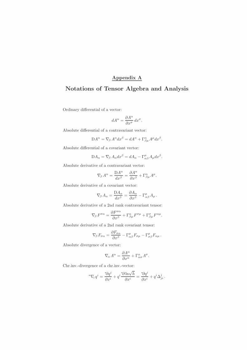
Appendix A

Notations of Tensor Algebra and Analysis

Ordinary differential of a vector:

dAα =∂Aα

∂xσdxσ .

Absolute differential of a contravariant vector:

DAα = ∇β Aαdxβ = dAα + ΓαβµAµdxβ .

Absolute differential of a covariant vector:

DAα = ∇β Aαdxβ = dAα − ΓµαβAµdxβ .

Absolute derivative of a contravariant vector:

∇βAα =DAα

dxβ=∂Aα

∂xβ+ ΓαβµA

µ.

Absolute derivative of a covariant vector:

∇βAα =DAαdxβ

=∂Aα∂xβ

− ΓµαβAµ .

Absolute derivative of a 2nd rank contravariant tensor:

∇β F σα =∂F σα

∂xβ+ ΓαβµF

σµ + ΓσβµFαµ.

Absolute derivative of a 2nd rank covariant tensor:

∇β Fσα =∂Fσα∂xβ

− ΓµαβFσµ − ΓµσβFαµ .

Absolute divergence of a vector:

∇αAα =∂Aα

∂xα+ ΓαασA

σ.

Chr.inv.-divergence of a chr.inv.-vector:

∗∇i qi =∗∂qi

∂xi+ qi

∗∂ ln√h

∂xi=

∗∂qi

∂xi+ qi∆j

ji .

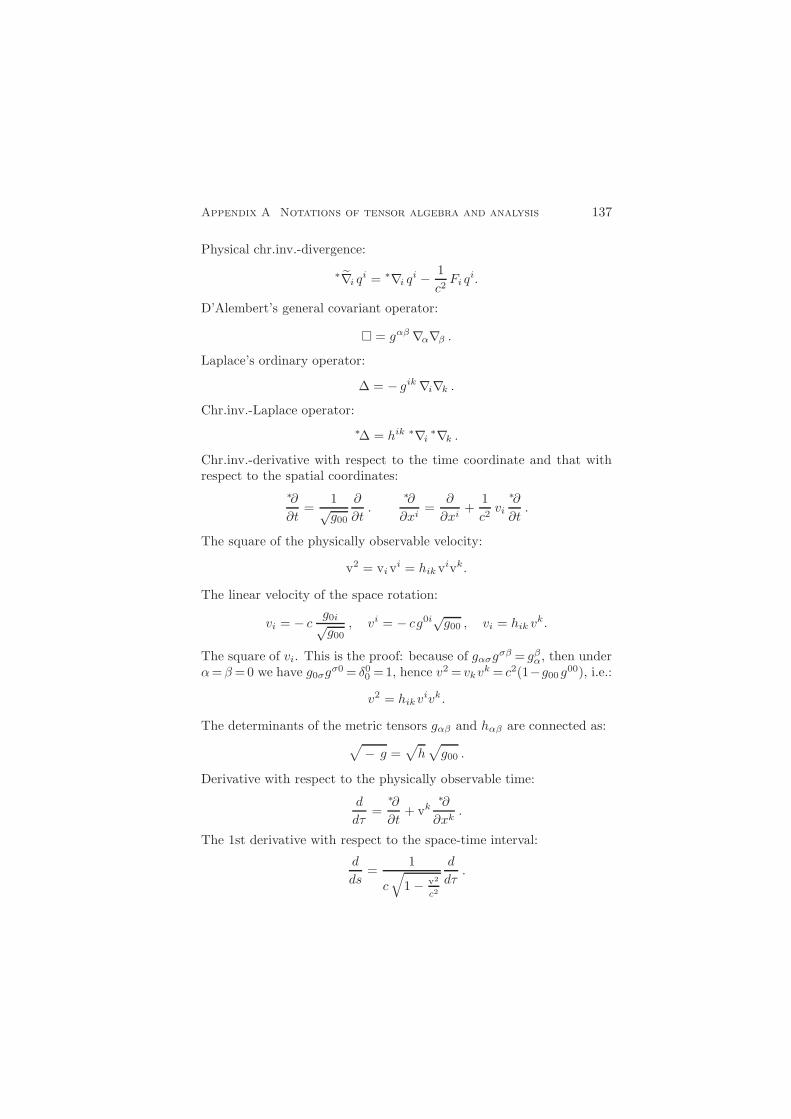
Appendix A Notations of tensor algebra and analysis 137

Physical chr.inv.-divergence:

∗∇i qi = ∗∇i qi −1

c2Fi q

i.

D’Alembert’s general covariant operator:

= gαβ∇α∇β .Laplace’s ordinary operator:

∆ = − gik∇i∇k .Chr.inv.-Laplace operator:

∗∆ = hik ∗∇i ∗∇k .Chr.inv.-derivative with respect to the time coordinate and that withrespect to the spatial coordinates:

∗∂

∂t=

1√g00

∂

∂t.

∗∂

∂xi=

∂

∂xi+

1

c2vi

∗∂

∂t.

The square of the physically observable velocity:

v2 = vivi = hik v

ivk.

The linear velocity of the space rotation:

vi = − cg0i√g00

, vi = − cg0i√g00 , vi = hik v

k.

The square of vi. This is the proof: because of gασgσβ = gβα, then under

α= β=0 we have g0σgσ0 = δ00 =1, hence v2 = vkv

k = c2(1−g00 g00), i.e.:

v2 = hikvivk.

The determinants of the metric tensors gαβ and hαβ are connected as:√

− g =√h√g00 .

Derivative with respect to the physically observable time:

d

dτ=

∗∂

∂t+ vk

∗∂

∂xk.

The 1st derivative with respect to the space-time interval:

d

ds=

1

c√1− v2

c2

d

dτ.

138 Appendix A Notations of tensor algebra and analysis

The 2nd derivative with respect to the space-time interval:

d2

ds2=

1

c2−v2d2

dτ2+

1

(c2−v2)2

(Dikv

ivk +vidvi

dτ+

1

2

∗∂hik∂xm

vivkvm)d

dτ.

The chr.inv.-metric tensor:

hik = − gik +1

c2vivk , hik = − gik, hki = δki .

Zelmanov’s relations between the Christoffel regular symbols and thechr.inv.-characteristics of the space of reference:

Dik +A·i

k· =c√g00

(Γi0k −

g0kΓi00

g00

),

giαgkβΓmαβ = hiqhks∆mqs , F k = − c2 Γk00

g00.

Zelmanov’s 1st identity and 2nd identity:

∗∂Aik∂t

+1

2

(∗∂Fk∂xi

−∗∂Fi∂xk

)= 0 ,

∗∂Akm∂xi

+∗∂Ami∂xk

+∗∂Aik∂xm

+1

2

(FiAkm + FkAmi + FmAik

)= 0 .

Derivative from v2 with respect to the physically observable time:

d

dτ

(v2)=

d

dτ

(hikv

ivk)= 2Dikv

ivk +∗∂hik∂xm

vivkvm+2vkdvk

dτ.

The completely antisymmetric chr.inv.-tensor:

εikm =√g00E

0ikm =e0ikm√h

, εikm =E0ikm√g00

= e0ikm√h .

Appendix B

A Thesis Presented at the April Meeting

2008 of the American Physical Society

2008 APS April MeetingApril 12–15, 2008, St. Louis, Missouri

Exact Solution for a Gravitational Wave Detector — by Dmitri

Rabounski and Larissa Borissova — The experimental statement on gravi-tational waves proceeds from the equation for deviating geodesic lines andthe equation for deviating non-geodesics. Weber’s result was not based uponan exact solution to the equations, but on an approximate analysis of whatcould be expected: he expected that a plane weak wave of the space met-ric may displace two resting particles with respect to each other. In thiswork, exact solutions are presented for the deviation equation of both freeand spring-connected particles. The solutions show that a gravitational wavemay displace particles in a two-particle system only if they are in motionwith respect to each other or the local space (there is no effect if they are atrest). Thus, gravitational waves produce a parametric effect on a two-particlesystem. According to the solutions, an altered detector construction can beproposed such that it might interact with gravitational waves: 1) a horizon-tally suspended cylindrical pig, whose butt-ends have basic relative oscilla-tions induced by a laboratory source; 2) a free-mass detector where suspendedmirrors have laboratory induced basic oscillations relative to each other.

Appendix C

A Thesis Presented at the March Meeting

2011 of the American Physical Society

2011 APS March MeetingMarch 21–25, 2011, Dallas, Texas

A Theory of Frozen Light According to General Relativity — by

Dmitri Rabounski and Larissa Borissova — We suggest a theory to frozenlight, which was first registered in 2000 by Lene Hau. Frozen light is explainedhere as a new state of matter. The explanation is given through space-timeterms of the General Theory of Relativity. We consider a fully degenerateregion of space (space-time), which is the ultimate case of the isotropic region(home of photons), where the metric is particularly degenerate. Both thespace-time interval, the observable time interval, and the observable three-dimensional interval are zero in a fully degenerate region. Therefore, we referto such a region and particles which inhabit it as zero-space and zero-particles.Moving to the coordinate quantities inside zero-space shows that real speedtherein is that of light, depending on the gravitational potential and therotation of space. It is shown that the eikonal equation for zero-particles is astanding wave equation: zero-particles are standing light waves, while zero-space is filled with a system of standing light waves (light-like hologram).With these, zero-particles appear to a regular (external) observer as merestopped light. This paper has been submitted to The Abraham Zelmanov

Journal.

Bibliography

1. Levi-Civita T. Nozione di parallelismo in una varieta qualunque e con-sequente specificazione geometrica della curvatura Riemanniana. Rendi-conti del Circolo Matematico di Palermo, 1917, tome 42, pages 173–205.

2. Zelmanov A. Chronometric invariants. Translated into English from thepreprint of 1944, American Research Press, Rehoboth (NM), 2006.

3. Zelmanov A. Chronometric invariants and accompanying frames of refer-ence in the General Theory of Relativity. Soviet Physics Doklady, MAIKNauka/Interperiodica, distributed by Springer, 1956, vol. 1, pages 227–230 (translated from Doklady Academii Nauk USSR, 1956, vol. 107, no. 6,pages 815–818).

4. Zelmanov A. On the relativistic theory of an anisotropic inhomogeneousuniverse. Translated from the manuscript of 1957, The Abraham Zelma-

nov Journal, 2008, vol. 1, pages 33–63.

5. Cattaneo C. General Relativity: relative standard mass, momentum, en-ergy, and gravitational field in a general system of reference. Nuovo Ci-

mento, 1958, vol. 10, pages 318–337.

6. Cattaneo C. Conservation laws in General Relativity. Nuovo Cimento,1959, vol. 11, pages 733–735.

7. Cattaneo C. On the energy equation for a gravitating test particle. Nuovo

Cimento, 1959, vol. 13, pages 237–240.

8. Cattaneo C. Problemes d’interpretation en Relativite Generale. ColloquesInternationaux du Centre National de la Recherche Scientifique, no. 170“Fluides et champ gravitationel en Relativite Generale”, Editions du Cen-tre National de la Recherche Scientifique, Paris, 1969, pages 227–235.

9. Hafele J. C. Relativistic behaviour of moving terrestrial clocks. Nature,July 18, 1970, vol. 227, pages 270–271.

10. Hafele J. C. Relativistic time for terrestrial circumnavigations. American

Journal of Physics, 1972, vol. 40, pages 81–85.

11. Hafele J. C. and Keating R.E. Around-the-world atomic clocks: predictedrelativistic time gains. Science, July 14, 1972, vol. 177, pages 166–168.

12. Hafele J. C. and Keating R.E. Around-the-world atomic clocks: observedrelativistic time gains. Science, July 14, 1972, vol. 177, pages 168–170.

13. Zelmanov A.L. Relationship of the orthometric monad formalism tochronometric and kinemetric invariants. Soviet Physics Doklady, MAIKNauka/Interperiodica, distributed by Springer, 1976, vol. 21, pages 147–150 (translated from Doklady Academii Nauk USSR, 1976, vol. 227, no. 1,pages 78–81).

142 Bibliography

14. Schouten J.A. und Struik D. J. Einfuhrung in die neuren Methoden derDifferentialgeometrie. Noordhoff, Groningen, 1938 (first published in Zen-

tralblatt fur Mathematik, 1935, Bd. 11 und Bd. 19).

15. Landau L.D. and Lifshitz E.M. The classical theory of fields. GITTL,Moscow, 1939. Referred with the 4th edition (expanded twice to the 1stedition of 1939), Butterworth–Heinemann, 1980. All the editions weretranslated in 1951–1980 by Morton Hamermesh.

16. Lie S. Theorie der Transformationsgruppen. First published by Teubner,Leipzig, in 3 volumes (vol. 1, 1888, 568 pages; vol. 2, 1890, 645 pages;vol. 3, 1893, 830 pages), reprinted by Chelsea Publishing — AmericanMathematical Society (NY), 1970, 2,043 pages.

17. Killing W. Uber die Grundlagen der Geometrie. Crelle’s Journal fur die

reine und angewandte Mathematik, Bd. 109, 1892.

18. Petrov A. Z. Einstein spaces. Pergamon Press, Oxford, 1969 (translatedby R.F.Kelleher, edited by J.Woodrow).

19. Rabounski D. and Borissova L. Exact theory to a gravitational wavedetector. New experiments proposed. Progress in Physics, 2006, vol. 2,pages 31–38.

20. Rabounski D. and Borissova L. Exact solution for a gravitational wavedetector. A presentation posted at the 2008 APS April Meeting, held inApril 12–15, 2008, in St. Louis, Missouri.

21. Borissova L. Gravitational Waves and Gravitational Inertial Waves Ac-cording to the General Theory of Relativity. The Abraham Zelmanov

Journal, 2010, vol. 3, pages 25–70

22. Weber J. General Relativity and gravitational waves. Interscience Pub-lishers, New York, 1961 (referred with the reprint by Dover Publications,Mineola, NY, 2004).

23. Synge J. L. Relativity: the general theory. North Holland, Amsterdam,1960 (referred with the 2nd edition, Foreign Literature, Moscow, 1963).

24. Weber J. Gravitational-wave-detector events. Physical Review Letters,1968, vol. 20, pages 1307–1308.

25. Weber J. Evidence for discovery of gravitational radiation. Physical Re-view Letters, 1969, vol. 22, pages 1320–1324.

26. Weber J. Gravitational radiation experiments. Physical Review Letters,1970, vol. 24, 276–279.

27. Borissova L. Quadrupole mass-detector in a field of weak plane gravita-tional waves. Russian Physics Journal, Springer New York, 1978, vol. 21,no. 10, pages 1341–1344 (translated from Izvestiya Vysshikh Uchebnykh

Zavedenii, Fizika, 1978, no. 10, pages 109–114).

28. Lefschetz S. Differential equations: geometric theory. Interscience Pub-lishers, New York, 1957.

Bibliography 143

29. Kamke E. Differentialgleichungen: Losungsmethoden und Losungen.Chelsea Publ. Co., New York, 1959.

30. Boschi D., Branca S., De Martini F., Hardy L., and Popescu S. Exper-imental realization of teleporting an unknown pure quantum state viadual classical and Einstein-Podolsky-Rosen Channels. Physical Review

Letters, 1998, vol. 80, pages 1121–1125.

31. Riebe M., Haffner H., Roos C. F., Hansel W., Benhelm J., Lancas-ter G.P.T., Korber T.W., Becher C., Schmidt-Kaler F., James D. F.V.,and Blatt R. Deterministic quantum teleportation with atoms. Nature,2004, vol. 429, pages 734–736.

32. Barrett M.D., Chiaverini J., Schaetz T., Britton J., Itano W.M.,Jost J.D., Knill E., Langer C., Leibfried D., Ozeri R., and Wineland D. J.Deterministic quantum teleportation of atomic qubits. Nature, 2004,vol. 429, pages 737–739.

33. Bennett C.H., Brassard G., Crepeau C., Jozsa R., Peres A., and Woot-ters W.K. Teleporting an unknown quantum state via dual classical andEinstein-Podolsky-Rosen channels. Physical Review Letters, 1993, vol. 70,pages 1895–1899.

34. Zelmanov A. L. On the formulation of the problem of the infinity of spacein the General Theory of Relativity. Soviet Physics Doklady, MAIKNauka/Interperiodica, distributed by Springer, 1959, vol. 4, pages 161–164 (translated from Doklady Academii Nauk USSR, 1959, vol. 124, no. 5,pages 1030–1033).

35. Rabounski D. Biography of Abraham Zelmanov (1913–1987). The Abra-

ham Zelmanov Journal, 2008, vol. 1, pages xx–xxvi.

36. Rabounski D. and Borissova L. A theory of frozen light according to Gen-eral Relativity. The Abraham Zelmanov Journal, 2011, vol. 4, pages 3–27.

37. Rabounski D. and Borissova L. A theory of frozen light according to Gen-eral Relativity. A presentation posted at the 2011 APS March Meeting,held in March 21–25, 2011, in Dallas, Texas.

38. Hau L.V., Harris S. E., Dutton Z., Behroozi C. H. Light speed reductionto 17 metres per second in an ultracold atomic gas. Nature, 18 February1999, vol. 397, 594–598.

39. Liu C., Dutton Z., Behroozi C.H., Hau L.V. Observation of coherentoptical information storage in an atomic medium using halted light pulses.Nature, 25 January 2001, vol. 409, 490–493.

40. Dutton Z., Budde M., Slowe C., Hau L.V. Observation of quantum shockwaves created with ultra-compressed slow light pulses in a Bose-Einsteincondensate. Science, 27 July 2001, vol. 293, 663–668.

41. Hau L.V. Frozen light. Scientific American, 17 July 2001, vol. 285, no. 1,52–59.

144 Bibliography

42. Hau L.V. Frozen light. Scientific American Special Edition “The Edge

of Physics”, 31 May 2003, 44–51.

43. Zhang R., Garner S.R., Hau L.V. Creation of long-term coherent opticalmemory via controlled nonlinear interactions in Bose-Einstein conden-sates. Physical Review Letters, 4 December 2009, vol. 103, 233602.

44. Phillips D. F., Fleischhauer A., Mair A., Walsworth R. L., Lukin M.D.Storage of light in atomic vapor. Physical Review Letters, 29 January2001, vol. 86, no. 5, 783–786.

45. Turukhin A.V., Sudarshanam V. S., Shahriar M. S., Musser J.A., HamB. S., Hemmer P.R. Observation of ultraslow and stored light pulses in asolid. Physical Review Letters, 14 January 2002, vol. 88, no. 2, 023602.

46. Rabounski D. On the speed of rotation of isotropic space: insight into theredshift problem. The Abraham Zelmanov Journal, 2009, vol. 2, 208–223.

About the Authors

Dmitri Rabounski (b. 1965 in Moscow, Russia) was educated at the Mos-cow High School of Physics. Commencing in 1983, he was trained byProf. Kyril Stanyukovich (1916–1989), a prominent scientist in gaseousdynamics and General Relativity. He was also trained with Dr. Abra-ham Zelmanov (1913–1987), the famous cosmologist and researcher inGeneral Relativity. During the 1980’s, he was also trained by Dr. VitalyBronshten (1918–2004), the well-known expert in the physics of destruc-tion of bodies in atmosphere. Dmitri Rabounski has published about 30scientific papers and 6 books on General Relativity, gravitation, physicsof meteoroids, and astrophysics. In 2005, he started a new Americanjournal on physics, Progress in Physics, where he is the Editor-in-Chief.In 2008, he established The Abraham Zelmanov Journal, a new interna-tional journal of General Relativity, gravitation, and cosmology, wherehe is the Editor-in-Chief. He is currently continuing his scientific studiesas an independent researcher.

Larissa Borissova (b. 1944 in Moscow, Russia) was educated at the Fac-ulty of Astronomy, the Department of Physics of the Moscow StateUniversity. Commencing in 1964, she was trained by Dr. Abraham Zel-manov (1913–1987), a famous cosmologist and researcher in GeneralRelativity. She was also trained, commencing in 1968, by Prof. KyrilStanyukovich (1916–1989), a prominent scientist in gaseous dynamicsand General Relativity. In 1975, Larissa Borissova received the “candi-date of science” degree on gravitational waves (the Soviet PhD). She haspublished about 30 scientific papers and 6 books on General Relativityand gravitation. In 2005, Larissa Borissova became a co-founder andAssociate Editor of Progress in Physics, and is currently continuing herscientific studies as an independent researcher.

PARTILES HERE AND BEYOND

THE MIRROR

by Dmitri Rabounski and Larissa Borissova

This is a research on all kinds of particles, which could be conceivablein the space-time of General Relativity. In addition to mass-bearingparticles and light-like particles, zero-particles are predicted: suchparticles can exist in a fully degenerate space-time region (zero-space). Zero-particles seem as standing light waves, which travel inan instant (non-quantum teleportation of photons); they might beobserved in a further development of the “stopped light experiment”which was first conducted in 2000, at Harvard, USA. The theoreticalexistence of two separate regions in the space-time is also shown,where the observable time flows into the future and into the past(our world and the mirror world). These regions are separated bya space-time membrane wherein the observable time stops. A fewother certain problems are considered. It is shown, through Killing’sequations, that geodesic motion of particles is a result of stationarygeodesic rotation of the space which hosts them. Concerning thetheory of gravitational wave detectors, it is shown that both free-mass detectors and solid-body detectors may register a gravitationalwave only if such a detector bears an oscillation of the butt-ends.

ISBN 978-1-59973-264-0Third edition, revised and expandedAmerican Research Press, 2012, 145 pagesPrinted in the USA

US $36.00 / EUR e27.00

and beyond the mirror

Documents