anchoring the yield curve using survey expectations
TRANSCRIPT

Work ing PaPer Ser ieSno 1632 / F ebruary 2014
anchoring the yield curveuSing Survey exPectationS
Carlo Altavilla, Raffaella Giacominiand Giuseppe Ragusa
In 2014 all ECB publications
feature a motif taken from
the €20 banknote.
note: This Working Paper should not be reported as representing the views of the European Central Bank (ECB). The views expressed are those of the authors and do not necessarily reflect those of the ECB.

© European Central Bank, 2014
Address Kaiserstrasse 29, 60311 Frankfurt am Main, GermanyPostal address Postfach 16 03 19, 60066 Frankfurt am Main, GermanyTelephone +49 69 1344 0Internet http://www.ecb.europa.euFax +49 69 1344 6000
All rights reserved.
ISSN 1725-2806 (online)EU Catalogue No QB-AR-14-006-EN-N (online)
Any reproduction, publication and reprint in the form of a different publication, whether printed or produced electronically, in whole or in part, is permitted only with the explicit written authorisation of the ECB or the authors.This paper can be downloaded without charge from http://www.ecb.europa.eu or from the Social Science Research Network electronic library at http://ssrn.com/abstract_id=2381871.Information on all of the papers published in the ECB Working Paper Series can be found on the ECB’s website, http://www.ecb.europa.eu/pub/scientific/wps/date/html/index.en.html
AcknowledgementsWe would like to thank M. Bauer, J. Christensen, C. Favero, D. Giannone, A. Justiniano, M. Modugno, G. Rudebusch, K. Sheppard, K. Singleton as well as conference and seminar participants to the Society for Economic Dynamics, Cyprus, Econometric Society Summer Meeting, Malaga, European Central Bank, Bank of England, Oxford University, Bank of Italy, Luiss University, Autonoma Barcelona, Chicago Fed, St Louis Fed and San Francisco Fed. Raffaella Giacomini gratefully acknowledges support from the British Academy Mid-career Fellowship. The views expressed in this paper are those of the authors and do not necessarily reflect the views of the European Central Bank.
Carlo AltavillaEuropean Central Bank; e-mail: [email protected]
Raffaella GiacominiUniversity College London; e-mail: [email protected]
Giuseppe RagusaLuiss University; e-mail: [email protected]

Abstract
The dynamic behavior of the term structure of interest rates is difficult to replicate withmodels, and even models with a proven track record of empirical performance have underper-formed since the early 2000s. On the other hand, survey expectations are accurate predictorsof yields, but only for very short maturities. We argue that this is partly due to the ability ofsurvey participants to incorporate information about the current state of the economy as wellas forward-looking information such as that contained in monetary policy announcements. Weshow how the informational advantage of survey expectations about short yields can be exploitedto improve the accuracy of yield curve forecasts given by a base model. We do so by employinga flexible projection method that anchors the model forecasts to the survey expectations in seg-ments of the yield curve where the informational advantage exists and transmits the superiorforecasting ability to all remaining yields. The method implicitly incorporates into yield curveforecasts any information that survey participants have access to, without the need to explicitlymodel it. We document that anchoring delivers large and significant gains in forecast accuracyfor the whole yield curve, with improvements of up to 52% over the years 2000-2012 relative tothe class of models that are widely adopted by financial and policy institutions for forecastingthe term structure of interest rates.
JEL Classification Codes: G1; E4; C5Keywords: Term Structure Models; Exponential Tilting; Blue Chip Analysts Survey; Fore-
cast Performance; Monetary Policy Forward Guidance; Macroeconomic Factors
1

Non-technical summary
The term structure of interest rates contains crucial information for both policymakers’ and investors’ decisions. Yet, in spite of a vast and growing literature on yield curve modelling, no single approach has emerged that can accurately describe the dynamic behaviour of yields. The two broad classes of yield curve models are no-arbitrage dynamic latent factor models and the Dynamic Nelson and Siegel (DNS) model. These models share a similar state-space structure in which the yields depend on three dynamic latent factors (level, slope, and curvature), which are extracted from the cross-section of yields. Broadly speaking, their differences lie in the restrictions they impose on the model’s parameters.
This paper’s premise is that latent factor models neglect a key determinant of yield dynamics: expectations about future economic developments. It is a well-documented fact that expectations contained in survey data can accurately forecast key macroeconomic variables, such as GDP, inflation, and yields, especially at short forecast horizons, and several recent papers have utilised survey data in the analysis of the term structure of interest rates.
In contrast to the existing approaches in the literature, we do not incorporate survey data into the model, as we show that this makes very little difference to the model’s performance. Instead, we employ a formal “anchoring” method that anchors the model forecasts to the survey expectations in segments of the yield curve where the informational advantage exists and transmits the superior forecasting ability to the rest of the curve.
In essence, the anchoring constrains the dynamics of some yields to replicate those of the survey expectations and thus implicitly incorporates into the forecasts of the whole yield curve any information that survey participants have access to without the need to explicitly model it. This can include information about the current state of the economy that survey participants deem relevant for predicting future interest rates and that they potentially extract from large dimensional data sets. In this respect, the survey expectation offers the possibility to capture both observable and “hidden” factors that can explain yield curve dynamics. The survey expectation can also reflect additional useful information, such as nonlinearities (for example, the zero-lower bound constraint), structural change, and information about the future course of monetary policy that may be difficult to capture with existing backward-looking models. In this paper, we stress in particular the role played by the ability of survey participants to capture the kind of forward-looking information about interest rates that is increasingly contained in monetary policy announcements.
An important question we address is which segments of the yield curve one should anchor, as one typically has access to survey expectations about several points along the yield curve.
Moreover, survey expectations are not necessarily accurate, so it is desirable to shed some light on the link between the accuracy of the survey expectations and that of the resulting anchored forecast. Our main result is to show that the anchoring procedure results in an improvement in accuracy for the whole yield curve if the survey expectations one utilises are informationally efficient relative to the model-based forecasts they replace, which in practice corresponds to a testable encompassing condition. In our data, we found that the informational efficiency condition is satisfied only for the 3-month yield, so in practice we suggest anchoring the short end of the yield curve to the corresponding survey expectation and then adjusting all remaining yields in a formal way, which we make explicit below.
Using U.S. data, we conduct a thorough empirical evaluation of the out-of-sample forecasting performance of the anchoring method, which incorporates Blue Chip financial analysts’ monthly expectations about yields into yield curve forecasts based on the Dynamic Nelson and Siege (DNS) model. It is worth emphasising that, although we take the DNS model as a benchmark due to its popularity in the forecasting literature, the anchoring method is more generally valid and could be applied to any base model of the yield curve.
We find that the anchoring procedure results in forecasts that uniformly and significantly outperform those produced by several versions of the DNS model.
Although these improvements are important on their own, we provide further insight into the economic forces driving the superior performance of the anchored forecasts. We find that the anchored forecasts implicitly incorporate measures of real activity and forward-looking information contained in monetary policy announcements. The ability of the anchoring method to incorporate the information contained in monetary policy announcements, in particular, has two important implications. The first is that the anchoring method is likely to become even more useful as a practical tool for forecasters and central bankers in the future, now that forward guidance has been formally adopted by several central banks around the world, including the Federal Reserve, the Bank of England and the ECB. The second is that any successful attempt to explicitly model the dynamics of yields should acknowledge the value of forward-looking information.

1 Introduction
The term structure of interest rates contains crucial information for both policymakers’ andinvestors’ decisions. Yet, in spite of a vast and growing literature on yield curve modeling, nosingle approach has emerged that can accurately describe the dynamic behavior of yields. Thetwo broad classes of yield curve models are no-arbitrage dynamic latent factor models (Duffieand Kan (1996), Litterman et al. (1991), Dai and Singleton (2000)) and the Dynamic Nelsonand Siegel (DNS) model of Diebold and Li (2006). These models share a similar state-spacestructure in which the yields depend on three dynamic latent factors (level, slope, and curvature),which are extracted from the cross-section of yields. Broadly speaking, their differences lie inthe restrictions they impose on the model’s parameters. Although the latter have become theleading method for yield curve forecasting at many policy institutions (BIS (2005)) due to theirsuccessful empirical performance (Diebold and Li (2006)), one of the findings of this paper isthat their performance has deteriorated in recent years. The fact that the three-factor structureis not sufficient to capture the dynamics of yields has been documented before (e.g., Dieboldand Rudebusch (2012), Mönch (2008)), and a general consensus has emerged in the literaturethat one must look beyond the cross-section of yields to pin down the dynamic behavior ofinterest rates, for example, by enlarging the model’s information set with either observablemacroeconomic factors (Diebold et al. (2006), Ang and Piazzesi (2003), Hördahl et al. (2006),Rudebusch and Wu (2008), Mönch (2008), and Coroneo et al. (2013)) or latent “hidden” factors(Joslin et al. (2010) and Duffee (2011)).
This paper’s premise is that latent factor models neglect a key determinant of yield dynamics:expectations about future economic developments. It is a well-documented fact that expectationscontained in survey data can accurately forecast key macroeconomic variables, such as GDP,inflation, and yields, especially at short forecast horizons (Stark (2010) and Chun (2012)), andseveral recent papers have utilized survey data in the analysis of the term structure of interestrates. For example, Chun (2011) uses Blue Chip Financial Analysts (henceforth BC) forecastsas observable factors in a no-arbitrage dynamic latent factor model; Chernov and Mueller (2012)develop a model that incorporates survey expectations and links them to the “hidden factor” ofJoslin et al. (2010) and Duffee (2011); Van Dijk et al. (2012) use survey expectations to improveestimates of some parameters in the DNS model, and Kim and Orphanides (2012) use surveydata to overcome some small-sample estimation problems in no-arbitrage dynamic latent factormodels.
In contrast to the existing approaches in the literature, we do not incorporate survey data intothe model, as we show that a number of extensions of the DNS model, including one that utilizessurvey data, performed poorly in our sample. Instead, we employ a formal “anchoring” methodthat anchors segments of the yield curve forecasts to the corresponding survey expectationsabout yields and transmits the superior forecasting ability to the rest of the curve. In essence,the anchoring constrains the dynamics of some yields to replicate those of the survey expectationsand thus implicitly incorporates into the forecasts of the whole yield curve any information thatsurvey participants have access to without the need to explicitly model it. This can include
2

information about the current state of the economy that survey participants deem relevant forpredicting future interest rates and that they potentially extract from large dimensional datasets. In this respect, the survey expectation offers the possibility to capture both observableand “hidden” factors that can explain yield curve dynamics (as also argued by Duffee (2011)).The survey expectation can also reflect additional useful information, such as nonlinearities(for example, the zero-lower bound constraint), structural change, and information about thefuture course of monetary policy that may be difficult to capture with existing backward-lookingmodels. In this paper, we stress in particular the role played by the ability of survey participantsto capture the kind of forward-looking information about interest rates that is increasinglycontained in monetary policy announcements.
An important question we address is which segments of the yield curve one should anchor,as one typically has access to survey expectations about several points along the yield curve.Moreover, survey expectations are not necessarily accurate, so it is desirable to shed some lighton the link between the accuracy of the survey expectations and that of the resulting anchoredforecast. Our main result is to show that the anchoring procedure results in an improvementin accuracy for the whole yield curve if the survey expectations one utilizes are informationallyefficient relative to the model-based forecasts they replace, which in practice corresponds toa testable encompassing condition. In our data, we found that the informational efficiencycondition is satisfied only for the 3-month yield, so in practice we suggest anchoring the shortend of the yield curve to the corresponding survey expectation and then adjusting all remainingyields in a formal way, which we make explicit below. As a quick visualization of the effects ofanchoring, consider Figure 4, which shows that the method shifts an existing yield curve forecasttoward the actual realization, with sizable accuracy improvements that are particularly visiblein regions of the yield curve near the anchoring point.
The theoretical justification of the method is based on exponential tilting (see Robertson et al.(2005) and Giacomini and Ragusa (2013)). Here we establish a link between the presence ofan informational advantage of the surveys over model-based forecasts and the accuracy of theanchored forecast.
We conduct a thorough empirical evaluation of the out-of-sample forecasting performance ofthe anchoring method, which incorporates Blue Chip financial analysts’ monthly expectationsabout yields into yield curve forecasts based on the DNS model. It is worth emphasizing that,although we take the DNS model as a benchmark due to its popularity in the forecasting liter-ature, the anchoring method is more generally valid and could be applied to any base model ofthe yield curve.
We find that the anchoring procedure results in forecasts that uniformly and significantlyoutperform those produced by several versions of the DNS model, including ones that explicitlyincorporate macroeconomic factors or survey forecasts. The accuracy gains are sizable, averagingabout 30% and up to 52%. The anchored forecast is also the only one that was able to beat therandom walk over the period 2000-2012. These results are robust to considering a subsamplethat ends in 2008, which suggests that the good performance of our method is not solely driven
3

by the fact that survery participants correctly incorporate zero lower bound constraints. Thisis also the reason why we don’t consider in our comparison models that explicitly take the zerolower bound constraint into account (for an interesting recent example, see Christensen andRudebusch (2013)).
Although these improvements are important on their own, we provide further insight into theeconomic forces driving the superior performance of the anchored forecasts. We find that theanchored forecasts implicitly incorporate measures of real activity and forward-looking infor-mation contained in monetary policy announcements. The ability of the anchoring method toincorporate the information contained in monetary policy announcements, in particular, has twoimportant implications. The first is that the anchoring method is likely to become even moreuseful as a practical tool for forecasters and central bankers in the future, now that forwardguidance has been formally adopted by several central banks around the world, including theFederal Reserve, the Bank of England and the ECB. The second is that any successful attemptto explicitly model the dynamics of yields should acknowledge the value of forward-lookinginformation.
The paper is organized as follows. Section 2 documents the informational advantage of sur-veys over variants of the DNS model. Section 3 describes the anchoring method. Section 4contains the empirical results and Section 5 concludes. Appendix A describes the yield andmacroeconomic data; Appendix B reports the in-sample estimation results of the DNS model;and Appendix C discusses the BC survey data.
2 The informational advantage of surveys over models
We first introduce the DNS model and variants of the model that incorporate the informationcontained in macroeconomic factors or in survey data. We document that none of these modelswere able to outperform the random walk in recent years. We then show that survey expectationsof yields have an information advantage over the model-based forecasts, but only for the veryshort yield. We conclude by linking the informational advantage of surveys over models to theability of survey participants to capture forward-looking information such as that contained inmonetary policy announcements.
2.1 The DNS model and its variants
The DNS model introduced by Diebold and Li (2006) for a m-dimensional vector of yields yt
with typical element yt(τ), where τ is the maturity, is given by:
yt(τ) = β1t + β2t
�1− e
−λτ
λτ
�+ β3t
�1− e
−λτ
λτ− e
−λτ
�+ ut(τ), (1)
where the dynamic factors β1t, β2t, and β3t are interpreted as the level, slope, and the curvatureof the yield curve and λ is a calibrated parameter governing the exponential decay rate of thecoefficients. As in Diebold and Li (2006), we let λ = 0.069.
4

We consider two different specifications for the law of motion of the factors. In the first, thevector of factors βt+h, where h is the forecast horizon, follows the process
βt+h = C + Γβt + ηt+h, (2)
where C a 3 × 1 vector of constant, Γ is assumed to be diagonal and ηt+h ∼ N(0, S) withelements independent of each other and S diagonal. Although we do not report the results here,we also considered a non diagonal specification for Γ, but we found that it made little differenceto the conclusions.
In the second specification, the evolution of the factors depends on additional observableinformation Xt:
βt+h = C + Γβt + ΛXt + ηt+h. (3)
We consider three variants: 1) Xt = (f (real)t , f
(nominal)t ) where f
(real)t and f
(nominal)t are the first
two principal components extracted from the 23 macroeconomic variables listed in Appendix A.We denote them f
(real)t and f
(nominal)t based on the fact that the first principal component has
a high correlation with real variables (e.g., correlation 0.75 with Industrial Production) and thesecond has a high correlation with nominal variables; 2) Xt equals the consensus h-step-aheadforecast of inflation from the BC survey; and 3) Xt equals the consensus h-step-ahead forecastof the three-month yield from the BC survey.
Estimation of ((1)) proceeds in two stages. In the first stage, the cross-section of yields is usedto estimate β1t, β2t, and β3t at each time period t using ordinary least squares. The outcome ofthis first step is thus a times series of estimated factors βt = (β1t, β2t, β3t). In the second stage,the parameters of equation ((2)) (or, alternatively equation ((3))) are estimated regressing eachelement of βt on each element of βt−h and a constant.
The h-step-ahead conditional mean forecast of the yields at time t, µt+h, is obtained as:
µt+h = Zβt+h, Z =
1 1−e−λτ1
λτ11−e−λτ1
λτ1− e
−λτ1
1 1−e−λτ2
λτ21−e−λτ2
λτ2− e
−λτ2
...1 1−e−λτm
λτm1−e−λτm
λτm− e
−λτm
. (4)
where βt+h = C + Γβt, or, alternatively βt+h = C + Γβt + ΛXt. To derive the density forecastof yt+h, which is needed for the anchoring procedure, we assume that the pricing errors areindependent over t and are normally distributed:
ut ≡
ut(τ1)...
ut(τm)
∼ N(0, Q), Q = E[utu�t]
5

Under this assumption and under the specifications for βt given in ((2)) or ((3)), yt+h isconditionally normally distributed
yt+h :�ft(yt+h) ∼ N (ZΓβt, Σ), Σ = ZSZ
� + Q
�. t = 1, . . . , T.
In practice, we recursively estimate Σ from the residuals of ((1)) and from the residuals of ((2))or ((3)).
2.2 The forecasting performance of the DNS model and its variants
In this section, we document how the forecasting performance of the DNS model has deterioratedin the years after those considered by Diebold and Li (2006), who found that the model performedwell in the sample from 1985-2000. This has been noted before, for example, by Diebold andRudebusch (2012) and Mönch (2008). We complement their results by showing that augmentingthe DNS model to incorporate information extracted from macroeconomic data or surveys doesnot solve the problem.
We estimate the DNS models using the series of U.S. zero-coupon yields constructed in Gürkay-nak et al. (2007).1 We consider average-of-the-month data from January 1985 to December 2012on yields with the following maturities expressed in months: 6, 9, 12, 15, 18, 21, 24, 30, 36, 48,60, 72, 84, 96, 108, 120. We augment the yield data with the monthly time series of the 3-monthTreasury constant maturity rate from the FRED data set (code GS3M), which corresponds tothe rate forecasted by the BC analysts.2 In total we have a panel of 324 monthly observationson 17 yields.
We estimate the DNS model and its variants using an out-of-sample recursive scheme andconsider forecast horizons of 3-, 6-, 9- and 12-months ahead. The first estimation period usesdata from 1985:1 to 1999:12, and we evaluate the forecasts over the out-of-sample period 2000:1to 2012:12. We compare the mean squared forecast error (MSFE) of each variant of the DNSmodel to that of a random walk benchmark, which forecasts the yields as µt+h = yt. The MSFEfor the forecast of a yield of maturity τ at horizon h is given by:
MSFEh(τ) =1
T
�
t
(µt+h(τ)− yt+h(τ))2,
where T is the size of the out-of-sample portion of the sample, which in our case is T = 144−h.Figure 1 shows that the random walk substantially outperforms all versions of the DNS model.
This is generally true for all maturities and all forecast horizons, with a particularly poor perfor-mance for maturities around five years. The only exception appears to be the 10-year yield, forwhich the model performs as well as the random walk at the three-month horizon. This means
1A detailed description of the data is given in Appendix A. We also performed a similar exercise using theFama-Bliss data (from CRSP), which are only available for one- to five-year maturities, and obtained similarconclusions, which we do not report in the paper.
2We also conducted the analysis using end-of-the-month data and the 3-month yield from the Gürkaynak et al.(2007) data set and obtained qualitatively similar results, which we do not report in the paper.
6

Figure 1. Relative MSFE of DNS variants against the random walk
(a) Baseline DNS
Maturities
Rel
ative
MSF
E
0.5
1.0
1.5
2.0
2.5
3.0
3 6 9 12 15 18 21 24 30 36 48 60 72 84 96 120
3−step ahead6−step ahead9−step ahead12−step ahead
(b) DNS with macro factors
Maturities
Rel
ative
MSF
E
0.5
1.0
1.5
2.0
2.5
3.0
3 6 9 12 15 18 21 24 30 36 48 60 72 84 96 120
3−step ahead6−step ahead9−step ahead12−step ahead
(c) DNS with BC yield
Maturities
Rel
ative
MSF
E
0.5
1.0
1.5
2.0
2.5
3.0
3 6 9 12 15 18 21 24 30 36 48 60 72 84 96 120
3−step ahead6−step ahead9−step ahead12−step ahead
(d) DNS with BC Inflation
Maturities
Rel
ative
MSF
E
0.5
1.0
1.5
2.0
2.5
3.0
3 6 9 12 15 18 21 24 30 36 48 60 72 84 96 120
3−step ahead6−step ahead9−step ahead12−step ahead
Notes: The figure reports the ratios of the MSFE for each variant of the DNS model against theMSFE of the random walk for different maturities and forecast horizons. Values larger than 1indicate that the random walk outperforms the model.
7

that incorporating macroeconomic or survey-based information directly into the model does notimprove its performance.
We should point out that the poor out-of-sample performance of the DNS model in recentyears stands in contrast to its good in-sample performance, which we document in Appendix B.
2.3 Surveys win at short maturities
As discussed in the introduction, a well-known fact in the forecasting literature is that surveyparticipants, such as those participating in the BC survey that we consider in this paper, oftenproduce more accurate forecasts than those based on econometric models. Here we focus inparticular on the BC consensus forecasts of yields, which are available for maturities of 3, 6, 12,24, 60, and 120 months and forecast horizons of 3, 6, 9, and 12 months.
Figure 2 reports the relative forecast performance of the BC forecasts and the DNS forecasts,assessed using the encompassing test described in detail in Section 3.2. The figure shows thesequence of test statistics computed over time testing the null hypothesis that the 3-month-aheadBC forecasts for maturities 3, 6, 12, 24, 60 and 120 months encompasses the corresponding DNSforecast. The null hypothesis is rejected when the sequence of test statistics crosses the horizontalsolid line, which represents the critical value. The test clearly rejects the null of encompassingfor all but the 3-month maturity, suggesting that the BC forecasts are informationally efficientrelative to the DNS forecast only at the very short end of the yield curve.
One of the possible explanations for why the survey forecast of the 3-month yield has stronglyand consistently outperformed the model’s forecasts since 2000 is that this rate closely reactsto macroeconomic news. This information gap between surveys and models is likely to beparticularly large when the economic environment is changing quickly, making it more difficultfor an econometric model to incorporate the new information. In particular, the fact that theinformational efficiency of the BC forecasts relative to the model-based forecast is limited tothe 3-month yield could be due to the fact that this is the rate that more closely reacts tomonetary policy decisions. Indeed, the 3-month Treasury bill rate is usually used as a proxy forthe monetary policy rate in many macroeconomic models.
This conjecture is corroborated by looking at how model-based and survey-based forecastsrespond to monetary policy announcements that contain explicit reference to the likely futurepath of the short-term rate. There have been several instances of monetary policy statementscontaining forward-looking information of this kind in recent years, especially since the FederalReserve began adopting forward guidance as a policy measure. Figure 3 below shows how thesurvey- and model-based forecasts reacted to one particular episode of forward guidance. Thefigure reports the 1- to 4-quarter-ahead forecasts of the 3-month yield given by the model andthe surveys before and after the FOMC Statement of August 9, 2011, which stated that the“Committee currently anticipates that economic conditions [....] are likely to warrant exception-ally low levels for the federal funds rate at least through mid-2013”. The figure clearly shows thatbefore the announcement both the model and the survey participants predicted a rate increasefor the following year. However, after the announcement the surveys immediately incorporated
8

Figure 2. Relative performance of BC vs. DNS forecasts over time
Time
Valu
e of
enc
ompa
ssin
g st
atis
tics
2004 2006 2008 2010 2012
−50
510
15
3−month
6−month
12−month
24−month
60−month
120−month
Notes: The figure reports the sequence of test statistics for the time-varying encompassing testdescribed in Section 3.2, testing the null hypothesis that the BC forecast encompasses the DNSforecast, against the alternative hypothesis that it does not. The null hypothesis is rejectedwhen the sequence of test statistics crosses the horizontal solid line, which represents the criticalvalue (which equals 2.62 for test statistics computed over an estimation window that uses 40%of the out-of-sample observations and for a 5% significance level).
9

Figure 3. The informational advantage of surveys over models
! " # $ % ! " # $ % ! " # $ % ! " # $ % ! " # $ % ! " # $&
&'"
&'$
&'(
&')
!
!'"
%%%%%%%%%%%%%%%%*+,-%"&!!%%%%%%%%*+./%"&!!%%%%%%%%0+1'%"&!!%%%%%%%%2-34'%"&!!%%%%%%%%564'%"&!!%%%%%%%%789'%"&!!
%
%
2+:9-/;8<-.
Note: The figure reports the 1- to 4-quarter-ahead forecasts of the 3-month yield given by theDNS model and the BC survey before and after the FOMC Statement of August 9, 2011.
the information about the policy decision to keep the rate fixed, whereas the model continued topredict a rate hike for several months afterwards, an increase that didn’t materialize. The abilityto quickly incorporate this information gave the survey forecast a clear accuracy gain, and thisis likely to have occurred on several other occasions during the period that we considered, whichwas characterized by several episodes of forward guidance.
In closing this section, it is important to emphasize that the informational advantage of thesurvey expectations is not due to a misalignment of the information sets on which the surveyand the model forecasts are based. As we explain in Appendix B, we were careful in matchingthe timing of the two forecasts. Appendix B also explains how we transformed the quarterly BCforecasts into monthly forecasts.
3 Anchoring the yield curve to survey expectations
The previous section showed that survey participants can have an informational advantage overmodel-based forecasts, but this is only true for the very short end of the yield curve. This meansthat, on one hand, survey expectations alone cannot be used to produce accurate forecasts ofthe entire yield curve and, on the other hand, that model-based forecasts cannot be entirely
10

discarded. In this section, we illustrate an anchoring method for incorporating the informationcontained in the survey expectations of the short yield into an existing model-based forecast ofthe yield curve.
3.1 The anchoring method
The method is presented without reference to a specific forecasting model, as it can be appliedto any model that provides a density forecast. We make the simplifying assumption that thesequence of h-step- ahead density forecasts for the vector of yields is normal with (conditional)mean µt+h and variance Σt+h,3
yt+h :�ft(yt+h) ∼ N (µt+h, Σt+h)
�. t = 1, . . . , T.
At time t, we observe the h-step ahead survey forecast for yields for the first r < m maturities(τ1, . . . , τr), that we denote as µt+h,1:r.4 Let yt,1:r denote the r × 1 subvector of yt containingyields at maturities (τ1, τ2, . . . , τr).
We approach the problem of incorporating µt+h,1:r into the forecast from an informationtheoretic point of view, by projecting the density forecast ft onto the space of densities thathave conditional mean equal to the survey forecasts for maturities τ1, . . . , τr. More formally, thisset of densities can be characterized as
�Ht+h =
�ht :
�yt+h,1:rht(yt+h)dyt+h = µt+h,1:r
�.
It is important to note that no constraints are imposed on the forecasts of yields at longermaturities, τr+1, . . . , τm. The idea is to select the density in �Ht+h that is "closest" to themodel-based density forecast ft, where closeness is measured by the Kullback-Leibler informationcriterion. We seek a solution to the following minimization problem
h∗t (yt+h) = arg min
h∈ �Ht+h
�log
�ht(u)
ft(u)
�ht(u)du. (5)
Minimization problems such as ((5)) play an important role in statistics and econometrics(Csiszár (1975); ?; Kitamura and Stutzer (1997); Newey and Smith (2004); Ragusa (2011)), andthey have been considered in the forecasting literature by Robertson et al. (2005) and Giacominiand Ragusa (2013). Any of the previous references show that the solution is a new multivariatedensity taking the form
h∗t (yt+h) = exp
�ζt + ξ
�t [yt+h,1:r − µt+h,1:r]
�ft(yt+h),
where ζt and ξt are parameters chosen in such a way that h∗t (yt+h) ∈ �Ht+h. For the special case3See Giacomini and Ragusa (2013) for the general case of a nonnormal density forecast.4In the interest of notational clarity, we consider only the case in which the survey forecasts considered are for
maturities τ1, τ2, . . . , τr. It is, however, immediate to extend the results of this section to cases in which surveyforecasts of noncontiguous maturities are considered.
11

of a base density that is multivariate normal, Giacomini and Ragusa (2013) show that we havethe following analytical expression for h
∗t (yt+h):
h∗t (yt+h) = (2π)−
m2
���Σt+h
���−
12exp
�−1
2(yt+h − µ
∗t+h)
�Σ−1t+h(yt+h − µ
∗t+h)
�,
with
µ∗t+h =
µt+h,1:r
µt+h,r+1:m − Σt+h,21
�Σt+h,11
�−1(µt+h,1:r − µt+h,1:r)
and Σt+h,11 and Σt+h,21 are blocks of the partitioned matrix Σt+h:
Σt+h =
Σt+h,11r×r
Σt+h,12r×(m−r)
Σt+h,21(m−r)×r
Σt+h,22(m−r)×(m−r)
.
Thus, the solution to ((5)) is a normal density with the same variance as the initial fore-cast density, Σt+h, but a mean that is equal to the survey forecast for those yields that aredirectly restricted, and for the remaining yields it is equal to a combination between the modelforecast and the discrepancy between the survey and the restricted model forecasts. The ef-fect of anchoring the first r yields to the survey forecasts on the other yields depends on thisdiscrepancy and on Σt+h. Forecasts of yields at different maturities are generally positivelycorrelated. This implies that when the model forecast is larger than that of the survey, that is,when µt+h,1:r − µt+h,1:r > 0, µt+h,r+1:N is adjusted downwards; on the other hand, when themodel forecast is smaller than the survey, µt+h,r+1:N is increased.
3.2 Where to anchor the yield curve?
A natural question to ask is which survey data one should use to anchor the yield curve, giventhat the survey expectations are in principle available for a number of yields. In this section, weprovide guidance on where to anchor the yield curve by showing that, if the survey expectationof a given yield is informationally efficient relative to the corresponding model-based forecast,using this expectation to anchor the yield curve delivers an improvement in forecast accuracyfor the yield curve as a whole. The notion of informational efficiency is equated here to forecastencompassing, which conveniently lends itself to developing a testable condition that can beused to decide which survey data to use for anchoring.
Formally, we have the following result:
Proposition 1. Let et+h(τ) and et+h(τ) denote the model- and the survey-based h-step-aheadforecast errors for a yield with maturity τ , respectively. If the survey expectation for the yield of
12

maturity τ encompasses the model-based forecast of the same yield, that is, if
E [(et+h(τ)− et+h(τ))et+h(τ)] ≤ 0, (6)
then the anchored density forecast h∗t (yt+h) is more accurate than the base forecast ft(yt+h),
according to the logarithmic scoring rule of Amisano and Giacomini (2007), i.e.,
E
�log
�h∗t (yt+h)
ft(yt+h)
��> 0. (7)
Proof. Since
E
�log
�h∗t (yt+h)
ft(yt+h)
��= E [ζt + ξtet+h(τ)] ,
it is sufficient to show that the expectations of both terms are positive. In particular, we showthat ξt = Σ−1
t+h,11(µt+h(τ) − µt+h(τ)) and ζt = 12 Σ
−1t+h,11(µt+h(τ) − µt+h(τ))2, from which it
follows that E [ζt] ≥ 0, and that E [ξtet+h(τ)] = E
�Σ−1t+h,11(et+h(τ)− et+h(τ))et+h(τ)
�≥ 0 if
condition ((6)) is satisfied.Analytical expressions for ξt and ζt can be obtained by completing the square, as follows.
First write h∗t (yt+h) = exp {ζt + ξ
�t [yt+h(τ)− µt+h(τ)]} ft(yt+h) as
h∗t (yt+h) = (2π)−
m2
���Σt+h
���−
12
× exp
�−1
2(yt+h − µt+h)
�Σ−1t+h(yt+h − µt+h) + ζt + ξ
�t [Jyt+h − µt+h(τ)]
�,
where J is a selection vector selecting the element of yt+h corresponding to maturity τ . We have
−1
2(yt+h − µt+h)
�Σ−1t+h(yt+h − µt+h) + ζt + ξ
�t [Jyt+h − µt+h(τ)] = y
�t+hAyt+h + y
�t+hb+ c
where A = −12 Σ
−1t+h and b = Σ−1
t+hµt+h+J�ξt and c = −
12 µ
�t+hΣ
−1t+hµt+h− ξ
�tµt+h(τ)+ ζt. We can
thus write y�t+hAyt+h+y
�t+hb+c =
�yt+h +
12A
−1b��A�yt+h +
12A
−1b�+k with k = c−
14b
�A
−1b,
which gives
h∗t (yt+h) = (2π)−
m2
���Σt+h
���−
12exp(k)exp
��yt+h +
1
2A
−1b
��
A
�yt+h +
1
2A
−1b
��.
Imposing the constraint E [Jyt+h] = µt+h(τ) implies that −12JA
−1b=µt+h(τ), which in turn
gives ξt = Σ−1t+h,11(µt+h(τ)− µt+h(τ)). To obtain the expression for ζt, note that we must have
that k = 0 and thus set c = 14b
�A
−1b and solve for ζt to obtain, after a few straightforward
manipulations, ζt = 12 Σ
−1t+h,11(µt+h(τ)− µt+h(τ))2. This completes the proof.
Condition ((6)) can be empirically tested using a modification of the Giacomini and Rossi(2010) fluctuation test, which accounts for the possibility that the expectation might be changing
13

Table 1. Critical values for the encompassing test (kδ,α)
α δ
0.1 0.2 0.3 0.4 0.5 0.6 0.7 0.8 0.90.05 3.176 2.938 2.770 2.624 2.475 2.352 2.248 2.080 1.9750.10 2.928 2.676 2.482 2.334 2.168 2.030 1.904 1.740 1.600
over time.5
For ease of exposition, in the following we omit the reference to the forecast horizon h, withthe understanding that the size of the out-of-sample period T will be different for differentforecast horizons. The test takes as primitives two sequences of out-of-sample forecast errorsfor the survey forecast and for the model-based forecast, et(τ) and et(τ) for t = 1, ..., T. Atest of the null hypothesis (6) of encompassing, H0 : E [(et+h(τ)− et+h(τ))et+h(τ)] ≤ 0 againstthe one-sided alternative that the survey forecast does not encompass the model forecast can beobtained by letting ∆Lt=(et+h(τ)−et+h(τ))et+h(τ) in Giacomini and Rossi (2010)’s Fluctuationtest. The test is implemented by choosing a fraction δ of the total out-of-sample size T andcomputing a sequence of standardized rolling means of ∆Lt:
Ft,δ = σ−1(δT )−1/2
t�
j=t−δT+1
[(ej(τ)− ej(τ))ej(τ)] , t = δT, ..., T,
where σ is an HAC estimator of the standard deviation of (et+h(τ)− et+h(τ))et+h(τ) computedover the rolling window, typically with truncation lag h − 1, where h is the forecast horizon.The null hypothesis is rejected when
maxt≤T
Ft,δ > kδ,α,
where the critical value kδ,α is given in Table 1.
4 Empirical results
In this section, we apply the anchoring method described in Section 3 to the DNS model and the3-month yield BC forecast, which was the only forecast to satisfy the informational efficiencycondition discussed in Section 3.2. Our goal is to assess the out-of-sample performance of theindividual yield forecasts, relative to the DNS forecasts and to the random walk benchmark.
5Note that, even though Giacomini and Rossi (2010) restrict attention to a rolling window forecasting schemeto avoid the complications that arise when conducting pairwise comparisons of forecast accuracy in the context ofestimated nested models, the fact that one of our forecasts here is model-free prevents the need to limit attentionto the rolling scheme.
14

Recall that the anchored forecast for the whole vector of yields for forecast horizon h is given by
µ∗t+h =
µt+h,1
µt+h,2:m − Σt+h,21
�Σt+h,11
�−1(µt+h,1 − µt+h,1)
,
where µt+h,1 is the 3-month yield BC forecast, µt+h,2:m the vector of DNS forecasts for yieldswith maturity 6,...,120 months, Σt+h,11 and Σt+h,21 are blocks of the partitioned variance matrixΣt+h:
Σt+h =
Σt+h,11
1×1Σt+h,121×16
Σt+h,2116×1
Σt+h,2216×16
.
4.1 Anchoring works
Table 2 reports relative MSFE for the anchored forecasts against either the forecasts from thebase DNS model or the random walk benchmark, for each maturity and forecast horizon. Table3 reports the same results for a restricted sample that ends in 2008 and thus excludes thezero lower bound period. The asterisks indicate that the Diebold and Mariano (1995) testrejects the null of equal forecast accuracy at 10% against the alternative that the anchoredforecast is more accurate. The table clearly shows that the anchored forecasts significantly andstrongly outperform the DNS forecasts for almost all maturities and forecast horizons, witha typical forecast accuracy gain of about 30% and up to 52%. The only exception is for afew long maturities and short forecast horizons, at which the anchored forecasts and the DNSforecasts perform equally well. The table also gives evidence that the anchored method was ableto outperform the random walk, and significantly for maturities up to 15 months and forecasthorizons up to 6 months ahead, in a sample in which the DNS model and its variants consistentlyfailed, as shown in Figure 1. These conclusions are robust to excluding the zero lower boundperiod, suggesting that the superior performance of our method is not solely driven by theability of the survey expectations to incorporate the zero lower bound constraint. For space-saving reasons, we do not report the results of the comparison between the anchored forecastsand the variants of the DNS forecasts which incorporate macroeconomic information or surveyexpectations, but they paint a very similar picture and are available upon request.
Figure 4 reports the yield curve implied by the DNS and anchored forecast before and afterthe policy announcement of August 9, 2011, that was discussed in Figure 3. The figure showsthat, whereas before the announcement the DNS and anchored yield curve forecasts similarlyoverpredicted the actual yield curve, after the announcement the anchored forecast quicklyincorporates the information contained in the FOMC statement and shifts the entire yield curvedownwards towards the actual realization with a sizable adjustment relative to the previousmonth. The DNS forecasts, instead, continue to largely overpredict the actual yield curve. Thisshowcases the ability of the anchoring method to swiftly incorporate the informational advantagethat surveys have about short yields and transmit it to the rest of the curve.
15

Table 2. Relative MSFEs of anchored forecasts
Anchored vs DNS Anchored vs RWMaturity h=3 h=6 h=9 h=12 h=3 h=6 h=9 h=12
3 0.48∗ 0.53∗ 0.58∗ 0.67∗ 0.78∗ 0.83 0.90 1.006 0.49∗ 0.52∗ 0.57∗ 0.66∗ 0.62∗ 0.72∗ 0.81 0.939 0.54∗ 0.54∗ 0.59∗ 0.67∗ 0.71∗ 0.79∗ 0.87 0.9812 0.58∗ 0.57∗ 0.60∗ 0.68∗ 0.78∗ 0.84 0.92 1.0415 0.62∗ 0.59∗ 0.62∗ 0.69∗ 0.83∗ 0.89 0.97 1.0918 0.64∗ 0.61∗ 0.63∗ 0.70∗ 0.87 0.94 1.02 1.1521 0.66∗ 0.63∗ 0.64∗ 0.70∗ 0.91 0.98 1.07 1.2024 0.68∗ 0.64∗ 0.65∗ 0.71∗ 0.94 1.02 1.12 1.2630 0.70∗ 0.67∗ 0.67∗ 0.71∗ 1.01 1.10 1.22 1.3736 0.72∗ 0.69∗ 0.68∗ 0.72∗ 1.07 1.18 1.32 1.4848 0.75∗ 0.73∗ 0.70∗ 0.73∗ 1.16 1.28 1.47 1.6660 0.77∗ 0.75∗ 0.73∗ 0.74∗ 1.19 1.32 1.56 1.7872 0.80∗ 0.78∗ 0.74∗ 0.75∗ 1.17 1.31 1.57 1.8184 0.84∗ 0.81∗ 0.76∗ 0.76∗ 1.12 1.26 1.53 1.7796 0.89 0.84∗ 0.78∗ 0.76∗ 1.06 1.20 1.45 1.69108 0.95 0.87∗ 0.80∗ 0.77∗ 1.03 1.13 1.36 1.59120 1.00 0.90 0.82∗ 0.78∗ 1.02 1.08 1.27 1.48
Notes: The table reports the ratios of MSFE for the models considered. The asterisk indicatessignificance at 10%, according to the Diebold and Mariano (1995) test of equal accuracy againstthe alternative that the anchored forecast is more accurate. The Diebold and Mariano test wasimplemented using an HAC estimator with h− 1 truncation parameter.
Figure 4. DNS and Anchored forecasts before and after the monetary policy announcement
3 6 12 24 36 48 60 0
0.5
1
1.5
2
2.5
Yiel
d
Maturity
August 2011
3 6 12 24 36 48 60 0
0.2
0.4
0.6
0.8
1
1.2
1.4
1.6
1.8
2
Yiel
d
Maturity
September 2011
Nelson Siegel Tilted NS Data
Notes: The figure shows the 3-month-ahead yield curve forecast implied by the DNS model andthe corresponding anchored forecast made before and after the FOMC Statement of August 9,2011, together with the actual yield curve realization.
16
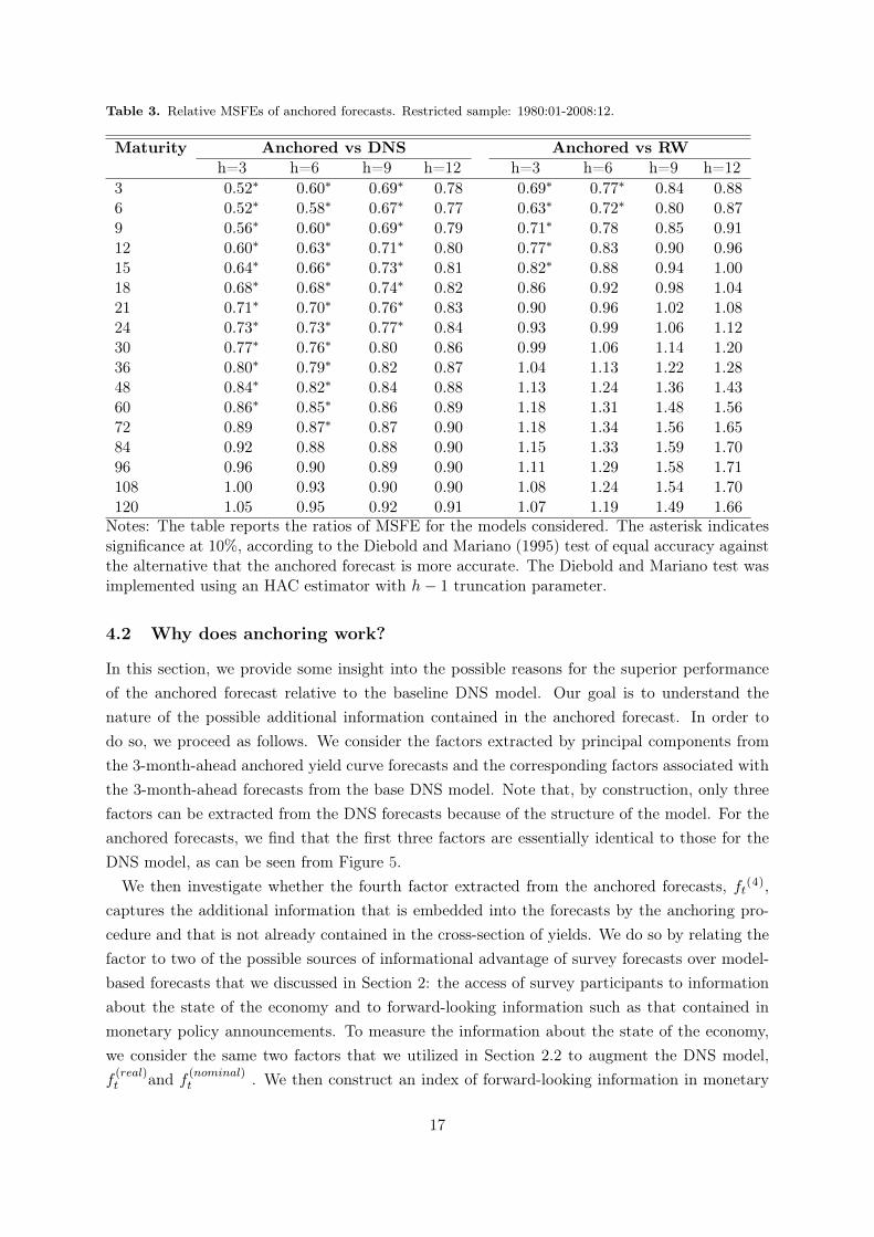
Table 3. Relative MSFEs of anchored forecasts. Restricted sample: 1980:01-2008:12.
Maturity Anchored vs DNS Anchored vs RWh=3 h=6 h=9 h=12 h=3 h=6 h=9 h=12
3 0.52∗ 0.60∗ 0.69∗ 0.78 0.69∗ 0.77∗ 0.84 0.886 0.52∗ 0.58∗ 0.67∗ 0.77 0.63∗ 0.72∗ 0.80 0.879 0.56∗ 0.60∗ 0.69∗ 0.79 0.71∗ 0.78 0.85 0.9112 0.60∗ 0.63∗ 0.71∗ 0.80 0.77∗ 0.83 0.90 0.9615 0.64∗ 0.66∗ 0.73∗ 0.81 0.82∗ 0.88 0.94 1.0018 0.68∗ 0.68∗ 0.74∗ 0.82 0.86 0.92 0.98 1.0421 0.71∗ 0.70∗ 0.76∗ 0.83 0.90 0.96 1.02 1.0824 0.73∗ 0.73∗ 0.77∗ 0.84 0.93 0.99 1.06 1.1230 0.77∗ 0.76∗ 0.80 0.86 0.99 1.06 1.14 1.2036 0.80∗ 0.79∗ 0.82 0.87 1.04 1.13 1.22 1.2848 0.84∗ 0.82∗ 0.84 0.88 1.13 1.24 1.36 1.4360 0.86∗ 0.85∗ 0.86 0.89 1.18 1.31 1.48 1.5672 0.89 0.87∗ 0.87 0.90 1.18 1.34 1.56 1.6584 0.92 0.88 0.88 0.90 1.15 1.33 1.59 1.7096 0.96 0.90 0.89 0.90 1.11 1.29 1.58 1.71108 1.00 0.93 0.90 0.90 1.08 1.24 1.54 1.70120 1.05 0.95 0.92 0.91 1.07 1.19 1.49 1.66
Notes: The table reports the ratios of MSFE for the models considered. The asterisk indicatessignificance at 10%, according to the Diebold and Mariano (1995) test of equal accuracy againstthe alternative that the anchored forecast is more accurate. The Diebold and Mariano test wasimplemented using an HAC estimator with h− 1 truncation parameter.
4.2 Why does anchoring work?
In this section, we provide some insight into the possible reasons for the superior performanceof the anchored forecast relative to the baseline DNS model. Our goal is to understand thenature of the possible additional information contained in the anchored forecast. In order todo so, we proceed as follows. We consider the factors extracted by principal components fromthe 3-month-ahead anchored yield curve forecasts and the corresponding factors associated withthe 3-month-ahead forecasts from the base DNS model. Note that, by construction, only threefactors can be extracted from the DNS forecasts because of the structure of the model. For theanchored forecasts, we find that the first three factors are essentially identical to those for theDNS model, as can be seen from Figure 5.
We then investigate whether the fourth factor extracted from the anchored forecasts, ft(4),captures the additional information that is embedded into the forecasts by the anchoring pro-cedure and that is not already contained in the cross-section of yields. We do so by relating thefactor to two of the possible sources of informational advantage of survey forecasts over model-based forecasts that we discussed in Section 2: the access of survey participants to informationabout the state of the economy and to forward-looking information such as that contained inmonetary policy announcements. To measure the information about the state of the economy,we consider the same two factors that we utilized in Section 2.2 to augment the DNS model,f(real)t and f
(nominal)t . We then construct an index of forward-looking information in monetary
17

Figure 5. Factors extracted from DNS and anchored forecasts
First factor
2000 2004 2008 2012
−10
−50
510
Second factor
2000 2004 2008 2012
−3−2
−10
12
3
Third factor
2000 2004 2008 2012
−0.6
−0.4
−0.2
0.0
0.2
0.4
Note: The figure shows the first 3 factors extracted from the DNS (solid line) and anchoredforecasts (dashed line).
policy announcements, I(forward)t , which equals one if in the month before the release of the sur-
vey forecast there was an FOMC statement that contained forward-looking information, whichwe assess by putting together Table 4 of Gürkaynak et al. (2007) for 2000:1 to 2004:12 andTable 1 of Campbell et al. (2012) for 2007:2011. For the years 2005 and 2006, we follow theconclusion by Kool and Thornton (2012) that there was no forward guidance during this periodand let the index equal zero. We then estimate the following regression (with t-statistics withinparentheses):
ft(4) = −0.05
(−0.5)− 0.37
(−5.7)f(real)t − 0.03
(−0.4)f(nominal)t + 0.41
(2.4)I(forward)t + error.
These estimates confirm that the superior accuracy of the anchored forecasts is related to theirability to incorporate information about real economic activity and forward-looking informationcontained in monetary policy announcements.
5 Conclusions
We proposed a formal and computationally simple anchoring method for incorporating surveyexpectations into a model-based forecast of the yield curve. The method constrains the dynamicsof some yields to replicate those of the survey expectations and implicitly incorporates into theforecasts of the whole yield curve any information that survey participants use without theneed to explicitly model it. We applied the method to the Dynamic Nelson and Siegel model of
18

Diebold and Li (2006) because of its popularity in financial and policy institutions, but we stressthat the method could be applied to the forecasts from any other base model. The method alsooffers a way to establish which information to incorporate, and we found grounds for using onlythe expectations about the three-month yield from the Blue Chip Financial Forecasts survey.
The results are stark. We find large and significant improvements in out-of-sample accuracyacross maturities and forecast horizons, with typical accuracy gains of about 30% and up to52% relative to the base model. To the best of our knowledge, our forecast is the only one thatwas able to outperform a random walk benchmark over the period 2000-2012, at least for shortmaturities and forecast horizons.
We provide an interpretation for the accuracy gains of the anchored forecasts and relate themto their ability to capture information about real economic activity as well as forward-lookinginformation contained in monetary policy announcements. This is likely to make the methodeven more relevant in the future given that several central banks such as the Federal Reserve,the European Central Bank, and the Bank of England are now adopting forward guidance as anonstandard monetary policy measure.
Finally, our method offers a way to formally incorporate into yield curve forecasts “hidden”or “unspanned” factors that go beyond the information contained in the cross-section of yields,and suggests that any successful attempt to explicitly model the dynamics of yields shouldacknowledge the value of forward-looking information.
19

Appendix
20

A Appendix. Yield and macroeconomic data
In this Appendix, we describe the data on the yields and the macroeconomic data that we usedin the paper.
The data on the yields used in the paper are pooled from two sources. The end-of-monththree-month yield is taken from the Fed’s H-15 release. For longer maturities, we use zero-coupon yields constructed in Gurkaynak et al. (2007). 6 We do not use the three-month yieldfrom this dataset because the BC explicitly asks participants to predict this particular rate. Wefocus on average-of-the-month data from January 1985 to December 2012. We consider yields ofthe following 17 maturities (in months): 3, 6, 9, 12, 15, 18, 21, 24, 30, 36, 48, 60, 72, 84, 96, 108,120. This choice provides us with a panel of 324 monthly observations on 17 different yields.Descriptive statistics of the sample are given in Table 4 and a plot of the data is in Figure 6.
The macroeconomic factors that appear in (3) are the first two principal components ex-tracted from a dataset of 23 variables. The dataset consists of monthly observations on 23 U.S.macroeconomic time series from 1985:1 through 2011:12. Table 5 lists the variables and the datatransformations that we applied to them.
Figure 6. Bond yields data in three dimensions.
Notes: The figure plots average-of-the-month U.S. Treasury bill and bond yields at maturitiesranging from 6 months to 10 years. The three-month yield is taken from the Fed’s H-15 release.For longer maturities, we use zero-coupon yields constructed in Gürkaynak et al. (2007). Thesample period is January 1985 through December 2012.
6This dataset is publicly available on the website of the Federal Reserve Board. The data can be obtained atthe address: http://www.federalreserve.gov/pubs/feds/2006/.
21
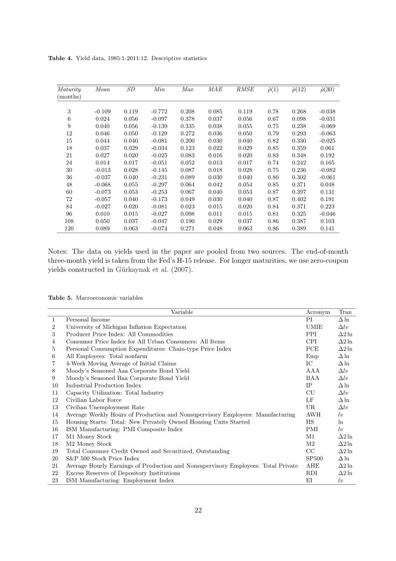
Table 4. Yield data, 1985:1-2011:12. Descriptive statistics
Maturity Mean SD Min Max MAE RMSE ρ(1) ρ(12) ρ(30)(months)
3 -0.109 0.119 -0.772 0.208 0.085 0.119 0.78 0.268 -0.0386 0.024 0.056 -0.097 0.378 0.037 0.056 0.67 0.098 -0.0319 0.040 0.056 -0.139 0.335 0.038 0.055 0.75 0.238 -0.06912 0.046 0.050 -0.129 0.272 0.036 0.050 0.79 0.293 -0.06315 0.044 0.040 -0.081 0.200 0.030 0.040 0.82 0.330 -0.02518 0.037 0.029 -0.034 0.123 0.022 0.029 0.85 0.359 0.06121 0.027 0.020 -0.025 0.083 0.016 0.020 0.83 0.348 0.19224 0.014 0.017 -0.051 0.052 0.013 0.017 0.74 0.242 0.16530 -0.013 0.028 -0.145 0.087 0.018 0.028 0.75 0.236 -0.08236 -0.037 0.040 -0.231 0.089 0.030 0.040 0.80 0.302 -0.06148 -0.068 0.055 -0.297 0.064 0.042 0.054 0.85 0.371 0.04860 -0.073 0.053 -0.253 0.067 0.040 0.053 0.87 0.397 0.13172 -0.057 0.040 -0.173 0.049 0.030 0.040 0.87 0.402 0.19184 -0.027 0.020 -0.081 0.023 0.015 0.020 0.84 0.371 0.22396 0.010 0.015 -0.027 0.098 0.011 0.015 0.81 0.325 -0.046108 0.050 0.037 -0.047 0.190 0.029 0.037 0.86 0.387 0.103120 0.089 0.063 -0.074 0.271 0.048 0.063 0.86 0.389 0.141
Notes: The data on yields used in the paper are pooled from two sources. The end-of-monththree-month yield is taken from the Fed’s H-15 release. For longer maturities, we use zero-couponyields constructed in Gürkaynak et al. (2007).
Table 5. Macroeconomic variables
Variable Acronym Tran1 Personal Income PI ∆ ln2 University of Michigan Inflation Expectation UMIE ∆lv3 Producer Price Index: All Commodities PPI ∆2 ln4 Consumer Price Index for All Urban Consumers: All Items CPI ∆2 ln5 Personal Consumption Expenditures: Chain-type Price Index PCE ∆2 ln6 All Employees: Total nonfarm Emp ∆ ln7 4-Week Moving Average of Initial Claims IC ∆ ln8 Moody’s Seasoned Aaa Corporate Bond Yield AAA ∆lv9 Moody’s Seasoned Baa Corporate Bond Yield BAA ∆lv10 Industrial Production Index IP ∆ ln11 Capacity Utilization: Total Industry CU ∆lv12 Civilian Labor Force LF ∆ ln13 Civilian Unemployment Rate UR ∆lv14 Average Weekly Hours of Production and Nonsupervisory Employees: Manufacturing AWH lv15 Housing Starts: Total: New Privately Owned Housing Units Started HS ln16 ISM Manufacturing: PMI Composite Index PMI lv17 M1 Money Stock M1 ∆2 ln18 M2 Money Stock M2 ∆2 ln19 Total Consumer Credit Owned and Securitized, Outstanding CC ∆2 ln20 S&P 500 Stock Price Index SP500 ∆ ln21 Average Hourly Earnings of Production and Nonsupervisory Employees: Total Private AHE ∆2 ln22 Excess Reserves of Depository Institutions RDI ∆2 ln23 ISM Manufacturing: Employment Index EI lv
22

Figure 7. Estimated DNS factors and empirical counterparts
Perc
ent
1985 1990 1995 2000 2005 2010
24
68
1012 Level factor
(y(3)+y(24)+y(120))/3
Perc
ent
1985 1990 1995 2000 2005 2010
−8−6
−4−2
02
4 Slope factory(3)−y(120)
Perc
ent
1985 1990 1995 2000 2005 2010
−2−1
01 0.37*Curvature factor
2 * y(24)−y(120)−y(3)
Note. The first factor β1t controls the yield curve level, as it can be verified that limτ→∞ yt(τ) =β1t. The second factor β2t is related to the yield curve slope, defined as the difference betweenthe 10-year and three-month yields. The third factor β3t governs the curvature of the yieldcurve, defined as twice the two-year yield minus the sum of the t10-year and three-month yields.
B Appendix. Estimation and in-sample fit of the DNS model
Here we report results regarding the estimation and the in-sample fit of the DNS model.Figure 7 shows the estimated time series of the three factors and their empirical counterparts.
The first graph plots the level factor (β1,t) against the average of short-, medium- and long-termyields, (yt(3) + yt(24) + yt(120))/3. The middle panel plots β2,t against the empirical slope ofthe yield curve yt(3)−yt(120). Finally, the bottom panel shows the behavior of 0.37β3,t and theempirical curvature proxy 2yt(24) − yt(3) − yt(120). The curvature factor closely matches thedynamics of its empirical counterpart: the difference between the two series has a mean of 2 basispoints and a standard deviation of 4 basis points. Also, the slope factor matches very closely theempirical proxy for the slope with a correlation of .99. The level factor shows instead a markeddeparture from the empirical counterpart. Importantly, this departure is most noticeable in theperiod 2000-2011. In particular, from January 1985 to December 2001, the correlation betweenβ1,t and (yt(3)+yt(24)+yt(120))/3 is 0.77, from January 2001 to December 2011 the correlationdrops to 0.24. The mean and standard deviations of the difference increase from 122 basis pointsto 216 basis points and from 99 basis points to 132 basis points, respectively.
23

Table 6. In-sample fit of the DNS model
Maturity Mean SD Min Max MAE ρ(1) ρ(12) ρ(30)(months)
3 -0.109 0.119 -0.772 0.208 0.085 0.78 0.268 -0.0386 0.024 0.056 -0.097 0.378 0.037 0.67 0.098 -0.0319 0.040 0.056 -0.139 0.335 0.038 0.75 0.238 -0.06912 0.046 0.050 -0.129 0.272 0.036 0.79 0.293 -0.06315 0.044 0.040 -0.081 0.200 0.030 0.82 0.330 -0.02518 0.037 0.029 -0.034 0.123 0.022 0.85 0.359 0.06121 0.027 0.020 -0.025 0.083 0.016 0.83 0.348 0.19224 0.014 0.017 -0.051 0.052 0.013 0.74 0.242 0.16530 -0.013 0.028 -0.145 0.087 0.018 0.75 0.236 -0.08236 -0.037 0.040 -0.231 0.089 0.030 0.80 0.302 -0.06148 -0.068 0.055 -0.297 0.064 0.042 0.85 0.371 0.04860 -0.073 0.053 -0.253 0.067 0.040 0.87 0.397 0.13172 -0.057 0.040 -0.173 0.049 0.030 0.87 0.402 0.19184 -0.027 0.020 -0.081 0.023 0.015 0.84 0.371 0.22396 0.010 0.015 -0.027 0.098 0.011 0.81 0.325 -0.046108 0.050 0.037 -0.047 0.190 0.029 0.86 0.387 0.103120 0.089 0.063 -0.074 0.271 0.048 0.86 0.389 0.141
Table 7. In-sample fit statistic of the DNS model. The model is estimated using monthly yield data fromJanuary 1985 to December 2011 with λt fixed at 0.0609. The descriptive statistics refer to the correspondingresiduals at various maturities. The last three columns present residual sample autocorrelations at lag 1, 12, and30, respectively.
Table 7 presents summary statistics of the residuals for each of the 17 maturities considered.Both the mean and the standard deviations of the residuals are small for all maturities. Thelargest means are observed at the shortest and longest maturities, respectively 11 and 9 basispoints. For the other maturities, the residual means oscillate between 1.4 and 7 basis points.Similarly, the residuals’ standard deviation is fairly stable, with largest values at the beginningand at the end of the curve.
24

C Appendix. Survey data
The empirical analysis in the paper considers survey expectations about interest rates
collected in the Blue Chip Financial Forecasts (BC). Each month, the BC publishes the
forecasts made by approximately 50 professional forecasters at leading consulting firms,
investment banks, and academic institutions. The interest rates that the BC analysts
forecast are the quarterly average of constant maturity Treasury yields as defined by the
Federal Reserve Statistical Release H.15.
There are two important issues to consider when comparing the accuracy of survey data
to that of model-based forecasts: the alignment of information sets and the conversion
of quarterly forecasts into monthly forecasts. Here we explain how we dealt with both
issues.
First, in order to guarantee a fair comparison between model and survey forecasts, we
made sure that the information sets on which the forecasts are based are aligned. In
particular, one must pay attention to the timing of the survey in relation to the type of
data used. For example, if the model is estimated using end-of-the-month data and the
survey is released around the 15th of the month (which is the typical release date for
the quarterly Survey of Professional Forecasters conducted by the Federal Reserve Bank
of Philadelphia), the informational advantage of the survey might be simply related to
the fact that when panelists submit their forecasts they have access to more information
than the model. This is however less of a concern when using BC survey data, because
the survey is published on the 1st day of each month, and one can thus make the as-
sumption that the survey forecasts have access to the same information set than a model
estimated using end-of-the-month data (or possibly a smaller information set if the survey
participants communicate their forecasts a few days before the BC releases them).
The second issue is related to the discrepancy between the frequency of the survey
(monthly) and the frequency of the target variables’ predictions (quarterly). In fact, this
discrepancy introduces a time-variation in the information set that has to be taken into
account when analyzing the accuracy of the survey predictions at a monthly frequency.
Table 8 describes how we extracted monthly forecasts from the quarterly BC survey
expectations. Recall that the BC analysts are asked to predict the average value of
a target variable over the current and the following quarters. For this reason, we use
average-of-the-month data (although using end-of-the-month data does not significantly
alter our results). In practice, we use the expectation made for the current quarter as
the 3-months-ahead prediction. This means that for the survey released on the 1st of
January the implied 3-month-ahead forecast is given by the expected value for the current
quarter, i.e. the nowcast, contained in the survey (BCNow, Jan in the table). Similarly,
the 6- 9- and 12-month-ahead forecasts made on the 1st of January are retrieved from
the 1-, 2-, and 3-quarter-ahead forecasts contained in the survey (BCJan,1Q, BCJan,2Q
BCJan,3Q in the table).
25

Table 8. Extraction of monthly forecasts from quarterly BC forecasts
Time of forecast release Forecast horizon (h = months)h = 3 h = 6 h = 9 h = 12
January 1st BCNow
Jan BC1QJan BC2Q
Jan BC3QJan
February 1st BC1Q
Feb BC2QFeb BC3Q
Feb BC4QFeb
March 1st BC1Q
Mar BC2QMar BC3Q
Mar BC4QMar
April 1st BCNow
Apr BC1QApr BC2Q
Apr BC3QApr
References
Amisano, G. and R. Giacomini (2007): “Comparing density forecasts via weighted likelihoodratio tests,” Journal of Business & Economic Statistics, 25, 177–190. 1
Ang, A. and M. Piazzesi (2003): “A no-arbitrage vector autoregression of term structuredynamics with macroeconomic and latent variables,” Journal of Monetary economics, 50,745–787. 1
BIS (2005): “Zero-Coupon Yield Curves: Technical Documentation,” BIS papers, 25. 1
Campbell, J. R., C. L. Evans, J. D. Fisher, and A. Justiniano (2012): “MacroeconomicEffects of FOMC Forward Guidance,” . 4.2
Chernov, M. and P. Mueller (2012): “The term structure of inflation expectations,” Journalof financial economics. 1
Christensen, J. H. and G. D. Rudebusch (2013): “Estimating shadow-rate term structuremodels with near-zero yields,” Federal Reserve Bank of San Francisco Working Paper Series,7. 1
Chun, A. L. (2011): “Expectations, bond yields, and monetary policy,” Review of FinancialStudies, 24, 208–247. 1
——— (2012): “Forecasting Interest Rates and Inflation: Blue Chip Clairvoyants or Economet-rics?” in EFA 2009 Bergen Meetings Paper. 1
Coroneo, L., D. Giannone, and M. Modugno (2013): “Unspanned Macroeconomic Factorsin the Yields Curve,” Tech. rep., ULB–Universite Libre de Bruxelles. 1
Csiszár, I. (1975): “I-divergence geometry of probability distributions and minimization prob-lems,” The Annals of Probability, 146–158. 3.1
26

Dai, Q. and K. J. Singleton (2000): “Specification analysis of affine term structure models,”The Journal of Finance, 55, 1943–1978. 1
Diebold, F. X. and C. Li (2006): “Forecasting the term structure of government bond yields,”Journal of econometrics, 130, 337–364. 1, 2.1, 2.1, 2.2, 5
Diebold, F. X. and R. S. Mariano (1995): “Comparing Predictive Accuracy,” Journal ofBusiness & Economic Statistics, 13, 253–265. 4.1
Diebold, F. X. and G. D. Rudebusch (2012): Yield Curve Modeling and Forecasting: TheDynamic Nelson-Siegel Approach, Princeton University Press. 1, 2.2
Diebold, F. X., G. D. Rudebusch, and S. Boragan Aruoba (2006): “The macroeconomyand the yield curve: a dynamic latent factor approach,” Journal of econometrics, 131, 309–338.1
Duffee, G. R. (2011): “Information in (and not in) the term structure,” Review of FinancialStudies, 24, 2895–2934. 1
Duffie, D. and R. Kan (1996): “A yield-factor model of interest rates,” Mathematical finance,6, 379–406. 1
Giacomini, R. and G. Ragusa (2013): “Forecasting with judgment,” Mimeo. 1, 3.1
Giacomini, R. and B. Rossi (2010): “Forecast comparisons in unstable environments,” Journalof Applied Econometrics, 25, 595–620. 3.2
Gürkaynak, R. S., B. Sack, and J. H. Wright (2007): “The US Treasury yield curve:1961 to the present,” Journal of Monetary Economics, 54, 2291–2304. 2.2, 2, 4.2, ??, 4
Hördahl, P., O. Tristani, and D. Vestin (2006): “A joint econometric model of macroe-conomic and term-structure dynamics,” Journal of Econometrics, 131, 405–444. 1
Joslin, S., M. Priebsch, and K. Singleton (2010): “Risk premiums in dynamic termstructure models with unspanned macro risks,” Manuscript, Stanford University. 1
Kim, D. H. and A. Orphanides (2012): “Term structure estimation with survey data oninterest rate forecasts,” Journal of Financial and Quantitative Analysis, 47, 241–272. 1
Kitamura, Y. and M. Stutzer (1997): “An information-theoretic alternative to generalizedmethod of moments estimation,” Econometrica: Journal of the Econometric Society, 861–874.3.1
Kool, C. and D. L. Thornton (2012): “How Effective Is Central Bank Forward Guidance?”FRB of St. Louis Working Paper No 2012. 4.2
Litterman, R. B., J. Scheinkman, and L. Weiss (1991): “Volatility and the yield curve,”The Journal of Fixed Income, 1, 49–53. 1
27

Mönch, E. (2008): “Forecasting the yield curve in a data-rich environment: A no-arbitragefactor-augmented VAR approach,” Journal of Econometrics, 146, 26–43. 1, 2.2
Newey, W. K. and R. J. Smith (2004): “Higher order properties of GMM and generalizedempirical likelihood estimators,” Econometrica, 72, 219–255. 3.1
Ragusa, G. (2011): “Minimum divergence, generalized empirical likelihoods, and higher orderexpansions,” Econometric Reviews, 30, 406–456. 3.1
Robertson, J. C., E. W. Tallman, and C. H. Whiteman (2005): “Forecasting UsingRelative Entropy,” Journal of Money, Credit and Banking, 37, 383–401. 1, 3.1
Rudebusch, G. D. and T. Wu (2008): “A Macro-Finance Model of the Term Structure,Monetary Policy and the Economy*,” The Economic Journal, 118, 906–926. 1
Stark, T. (2010): “Realistic evaluation of real-time forecasts in the Survey of ProfessionalForecasters,” Federal Reserve Bank of Philadelphia Research Rap, Special Report. 1
Van Dijk, D., S. J. Koopman, M. Van der Wel, and J. Wright (2012): “ForecastingInterest Rates with Shifting Endpoints,” Tinbergen Institute Discussion Paper 12-076/4. 1
28