anand bhaskar in -...
TRANSCRIPT
Statistical, algorithmic, and robustness aspects of population demographicinference from genomic variation data
by
Anand Bhaskar
A dissertation submitted in partial satisfaction of the
requirements for the degree of
Doctor of Philosophy
in
Computer Science
in the
Graduate Division
of the
University of California, Berkeley
Committee in charge:
Professor Yun S. Song, ChairProfessor Steven N. Evans
Professor Montgomery SlatkinProfessor David Tse
Fall 2013

Statistical, algorithmic, and robustness aspects of population demographicinference from genomic variation data
Copyright 2013by
Anand Bhaskar

1
Abstract
Statistical, algorithmic, and robustness aspects of population demographic inference fromgenomic variation data
by
Anand Bhaskar
Doctor of Philosophy in Computer Science
University of California, Berkeley
Professor Yun S. Song, Chair
The recent availability of large-sample high-throughput sequencing data has given usan unprecedented opportunity to very finely resolve the details of historical demographicprocesses that have shaped the genomes of modern human populations. Such understandingof population demography is important for several applications — to avoid false positivesin genome-wide association studies; to calibrate null models of neutral genome evolution inorder to find regions under selection; to study the impact of bottlenecks and small founderpopulations on genetic mutational load; to reconstruct large-scale historical human migrationand admixture events; and so on.
In this dissertation, we consider some statistical, algorithmic and robustness aspects ofdemographic inference from genomic variation data. In particular, we study the problem ofdetermining the historical effective size of a population from the sample frequency spectrum(SFS), which measures the distribution of allele frequencies in a sample of sequences drawnfrom the population.
From the statistical or information-theoretic perspective, it is known that this inverseproblem does not have a unique solution in general, no matter how large the sample size.For any population allele frequency distribution, there exist infinitely many population sizefunctions that are consistent with this distribution. While such a non-identifiability resultmight appear to pose a serious problem to statistical inference algorithms, we show thatthe situation is not so bad in practice. In particular, we prove that if the true populationsize function is piecewise-defined with each piece belonging to some family of biologically-motivated functions, then the SFS of a finite sample of sequences uniquely determines theunderlying demography. We obtain a general bound on the sample size sufficient for iden-tifiability; this bound depends on the number of pieces in the demographic model and onthe family of functions for each piece. We also give concrete instantiations of this boundfor piecewise-constant and piecewise-exponential models that are commonly used in demo-graphic inference analyses.

2
From the algorithmic perspective, we build on analytic results for the expected SFS of atime-varying population size function and develop an efficient likelihood-based algorithm toinfer piecewise-exponential population size histories from large sample allele frequency data.By considering very large samples, our method can resolve details of the population historyfrom the very recent past that are not otherwise accessible using smaller samples.
The third aspect of this dissertation is concerned with understanding the robustnessof widely used evolutionary models to violations of model assumptions. Continuous-timeevolutionary models like Kingman’s coalescent and its dual diffusion process are derived fromdiscrete models of random mating by assuming that the sample size being analyzed is muchsmaller than the the population size. However, the very large sample datasets being produceddue to advances in high-throughput sequencing technologies are approaching the limits of thisassumption. To investigate this issue, we develop exact algorithms for computation underthe discrete-time Wright-Fisher model and use these algorithms to study the distortions inseveral genealogical quantities arising due to the coalescent approximation. Our findingsindicate that for several demographic models inferred from large-scale sequence data, therecan be substantial genealogical deviations introduced by the coalescent approximation thatmight influence the results of inference studies.

i
To appa and amma, for instilling in me the importance of learning.

ii
Contents
1 Introduction 11.1 Motivation . . . . . . . . . . . . . . . . . . . . . . . . . . . . . . . . . . . . . 11.2 Demographic inference . . . . . . . . . . . . . . . . . . . . . . . . . . . . . . 2
1.2.1 Importance of understanding demography . . . . . . . . . . . . . . . 21.2.2 Representations of genomic data . . . . . . . . . . . . . . . . . . . . . 2
1.3 Preliminaries . . . . . . . . . . . . . . . . . . . . . . . . . . . . . . . . . . . 41.3.1 Wright-Fisher model . . . . . . . . . . . . . . . . . . . . . . . . . . . 41.3.2 Kingman’s coalescent . . . . . . . . . . . . . . . . . . . . . . . . . . . 51.3.3 Extension to variable population size . . . . . . . . . . . . . . . . . . 61.3.4 Sample frequency spectrum . . . . . . . . . . . . . . . . . . . . . . . 7
1.4 Overview . . . . . . . . . . . . . . . . . . . . . . . . . . . . . . . . . . . . . . 81.4.1 Statistical . . . . . . . . . . . . . . . . . . . . . . . . . . . . . . . . . 81.4.2 Algorithmic . . . . . . . . . . . . . . . . . . . . . . . . . . . . . . . . 91.4.3 Robustness . . . . . . . . . . . . . . . . . . . . . . . . . . . . . . . . 9
2 Identifiability of the population size function from SFS data 102.1 Overview . . . . . . . . . . . . . . . . . . . . . . . . . . . . . . . . . . . . . . 102.2 Notation . . . . . . . . . . . . . . . . . . . . . . . . . . . . . . . . . . . . . . 122.3 Main results . . . . . . . . . . . . . . . . . . . . . . . . . . . . . . . . . . . . 13
2.3.1 Determining expected times to the first coalescence event from the SFS 132.3.2 Piecewise population size models and sign change complexities . . . . 142.3.3 Identifiability from the SFS . . . . . . . . . . . . . . . . . . . . . . . 182.3.4 Extension to the folded frequency spectrum . . . . . . . . . . . . . . 22
2.4 The counterexample of Myers et al. . . . . . . . . . . . . . . . . . . . . . . . 242.5 Discussion . . . . . . . . . . . . . . . . . . . . . . . . . . . . . . . . . . . . . 25
3 Inference of the population size function from SFS data 273.1 Overview . . . . . . . . . . . . . . . . . . . . . . . . . . . . . . . . . . . . . . 273.2 Notation . . . . . . . . . . . . . . . . . . . . . . . . . . . . . . . . . . . . . . 293.3 Method . . . . . . . . . . . . . . . . . . . . . . . . . . . . . . . . . . . . . . 29
3.3.1 Poisson Random Field approximation . . . . . . . . . . . . . . . . . . 303.3.2 Computing the expected SFS under a variable population size . . . . 32

iii
3.4 Results . . . . . . . . . . . . . . . . . . . . . . . . . . . . . . . . . . . . . . . 34
4 Distortion of genealogical properties for very large sample sizes 414.1 Demographic models . . . . . . . . . . . . . . . . . . . . . . . . . . . . . . . 414.2 Multiple and simultaneous mergers in the DTWF model . . . . . . . . . . . 434.3 Number of lineages as a function of time . . . . . . . . . . . . . . . . . . . . 474.4 Expected sample frequency spectrum . . . . . . . . . . . . . . . . . . . . . . 474.5 A hybrid method for computing the frequency spectrum . . . . . . . . . . . 494.6 Computational details . . . . . . . . . . . . . . . . . . . . . . . . . . . . . . 49
4.6.1 Notation . . . . . . . . . . . . . . . . . . . . . . . . . . . . . . . . . . 494.6.2 Expected NLFT under the DTWF model . . . . . . . . . . . . . . . . 504.6.3 Expected number of multiple- and simultaneous-mergers in the DTWF
model . . . . . . . . . . . . . . . . . . . . . . . . . . . . . . . . . . . 504.6.4 Expected SFS under the DTWF model . . . . . . . . . . . . . . . . . 514.6.5 Expected NLFT under the coalescent . . . . . . . . . . . . . . . . . . 52
4.7 Dicussion . . . . . . . . . . . . . . . . . . . . . . . . . . . . . . . . . . . . . 53
5 Future directions 69
Bibliography 71
A Some identities related to Kingman’s coalescent 79A.1 Analytic expressions for the distribution of the coalescent waiting times . . . 79A.2 Expectation and standard deviation of the NLFT under the coalescent . . . 83

iv
Acknowledgments
It is hard to overstate the feelings of gratitude and respect I hold for my advisor, YunS. Song, who always provided me unrestrained freedom and encouragement to explore myinterests (both academic, and non-academic) and find my own path. Graduate school hasundoubtedly been one of the best experiences in my life so far, and I am certain that therapport I enjoyed with Yun has been a big reason for this. Yun has been an incrediblyinspiring role model and mentor who always amazes me with his ability to see the bigpicture even while tackling the devil in the technical details. Furthermore, I will considerit a great triumph if even a fraction of his work ethic has rubbed off on me. Many thanksare also due to Yun and his wonderful wife, Young, for introducing me to the delicacies ofKorean cuisine, and for so warmly and graciously hosting us graduate students at their houseon numerous occasions.
I am also grateful to the other members of my dissertation and qualifying examinationcommittees — Steve Evans, Monty Slatkin, Bernd Sturmfels, and David Tse. I am gratefulto Steve for patiently sharing his wealth of knowledge through several excellent courses; toMonty, for always offering an enthusiastic ear for my research ideas, and for providing sageadvice over the years; to Bernd, for inspiring my incipient interest in algebraic statisticsand geometry; and to David, with whom being a graduate student instructor was a funexperience.
Yun’s research group has always provided a very welcoming and collegial environmentto talk about research (and other unrelated topics). Ma’ayan Bresler, Andrew Chan, KelleyHarris, Paul Jenkins, Jack Kamm, Wei-Chun Kao, Joyce Liu, Jasmine Nirody, Joshua Paul,Sara Sheehan, Matthias Steinrucken, Jonathan Terhorst, Rachel Wang, and Junming Yin,it has been an honor learning from and working with you, and I really cherish the friendshipand camaraderie we’ve built over the years. I am also very thankful to Andy Clark, JackKamm, Uri Keich, Matthias Steinrucken, and Rachel Wang for their collaboration on severalresearch projects.
I would like to specially thank Uri Keich, whose kindness, patience and enthusiasm towork with me while I was still a clueless undergraduate student was extremely valuable formy development and self-confidence. Moreover, I am extremely grateful to Uri for alwaysgiving me candid advice, and for being instrumental in my decision to come to Berkeley. Iam also very grateful to Jayavel Shanmugasundaram and John Hopcroft for giving me myfirst tastes of undergraduate research.
I have often heard it said that graduate school can be a lonely experience. However, anincredible group of friends never let me see any truth in that statement. My office mates ofseveral years, Siu Man Chan, Siu On Chan, and Tom Watson have always regaled me withtheir stories and have been excellent buddies for jaunts around the Bay Area. My friends inthe theory group, especially James Cook, Anindya De, and Piyush Srivastava, have alwaysbeen a source of random interesting conversations. Longtime friends from high school inIndia and Singapore, and friends from Cornell have always kept me grounded and remindedme that there is a world outside academia. For this I would like to thank Devdeepta Bose,

v
Raquel Furtado, Nitesh Goel, Caitlin Heyden, Devashish Kumar, Aziz Lalljee, Maria Ligai,Nikhil Mehta, Rishi Ramchand, Chaitanya Reddy, Vikas Reddy, Corey Siegel, Byron Singh,Ted Suzman, Aditya Thatte, Tejas Viswanath, Ti Zhao, and several others. To my wonderfulformer housemates in Berkeley — Andrew Chan, Nicholas Kong, and Andrew Krioukov —thank you for being so easy-going and understanding even when I wasn’t always doing myshare of the chores.
Some of my most enjoyable experiences at Berkeley were the fantastic Russian languagecourses with Zachary Johnson, Mark Kaiser, and Lisa Little. Their passion and enthusiasmfor teaching have been truly inspirational. Захар, Марк и Лиза, спасибо вам за всё иизвините, что часто опаздывал на занятия. I am also very grateful to my Russian languageclassmate of several years, Jin Jin, who became one of my closest friends and introduced meto the amazing Berkeley Art Studio and Cal Performances.
I am grateful to the generous funding support provided by the Berkeley Fellowship duringmy initial years of graduate school. I am also thankful to La Shana Porlaris, Xuan Quach, andShirley Salanio for helping me with various administrative matters, and to Brian McClendonfor organizing many fantastic computational biology retreats.
Finally, and most importantly, I cannot thank my parents enough for giving me completefreedom to make my own decisions from a very early age. Their unconditional love andsupport mean the world to me and I am grateful to them each and every day for raising methe way they have. Amma and appa, this dissertation is dedicated to you.

1
Chapter 1
Introduction
1.1 Motivation
Human genetics has entered a new era with study sample sizes on the order of thousandsto tens of thousands of individuals sequenced at hundreds of genomic regions [1, 12, 19, 62,85]. A consistent finding arising from several large-sample studies is that human genomesharbor a substantial excess of rare variants compared to that predicted using previouslyapplied demographic models. For example, in a large-scale exome-sequencing study of 14,000individuals at over 200 genes, Nelson et al. [62] found that over 70% of the single nucleotidevariants only appear in one or two haplotypes in the sample, which corresponds to a minorallele frequency on the order of 0.01%. There are several factors that may contribute tothe discrepancy between observations in the data and theoretical predictions, including thefollowing possible explanations:
1. Previously applied demographic models are wrong. In particular, the observed poly-morphism patterns are indicative of a recent rapid growth in the effective populationsize, much more rapid than in previously applied demographic models. This conclusionwould be consistent with historical records of census population size [39].
2. Population substructure [71,81] and natural selection have distorted the observed poly-morphism patterns while previous demographic inference studies have failed to ade-quately account for these factors.
3. Theoretical predictions for a given demographic model are inaccurate when the samplesize is very large compared to the effective population size. Kingman’s coalescentprocess [44–46], which arises as a continuum limit of a large class of discrete-timerandom mating models [58, 59], provides an accurate approximation to these discrete-time models only if the sample size is sufficiently small compared to the effectivepopulation size. Violation of this assumption may distort the genealogical propertiesof a large sample in a way that may inflate rare variants relative to the predictions ofcoalescent theory.

CHAPTER 1. INTRODUCTION 2
The aim of this dissertation is to investigate the first and third possibilities in detailthrough the problem of demographic inference.
1.2 Demographic inference
1.2.1 Importance of understanding demography
Given a sample of genomic sequences from a large population, an important inference prob-lem with a wide variety of applications is to determine the underlying demography of thepopulation. Understanding the population demography is important for many reasons:
• Genome-wide association studies for inferring the genetic basis of complex heritablediseases can produce false positive associations if the demography of the population isnot taken into account properly [7, 10,53,65,70,86].
• The population demography is needed for calibrating correct null models of neutralgenome evolution so that one can conduct principled statistical tests to find regions ofthe genome that are subject to evolutionary pressure from natural selection [6, 49, 63,73,93].
• Genomic data can serve as an independent source of evidence for important anthro-pological events like population migrations, splits, admixture and introgression events[23,41,48,51,75,80,87] that have occurred in the history of our species.
• Demographic events such as bottlenecks and small founder populations can lead to ahigher frequency of deleterious mutations [49]. Conversely, increased genetic drift dueto bottlenecks might also serve as an explanation for speciation [2].
• Population demography is also important in forensic science applications, where a lowprobability of a random genetic profile from the population matching the crime scenesample is used as evidence for further investigation. This random match probabilitystrongly depends on the substructure and the amount of relatedness between individ-uals of the population [72].
1.2.2 Representations of genomic data
Demographic inference from full sequence data is a very challenging problem, and mostexisting methods for inferring demography can be broadly categorized into one of threetypes depending on the representation of the sequence data that they operate on.
Full sequence data
The evolution of full genomic sequences with intragenic recombination can be modeled usingrich generative processes like the coalescent with recombination [29, 37]. However, because

CHAPTER 1. INTRODUCTION 3
recombination induces correlations between distant genetic loci [94], it is computationallycumbersome to even simulate long sequences at many samples, let alone perform any kind ofinference from data. Several approximations to the coalescent with recombination have beenproposed which avoid these long-range correlations by assuming that the ancestral trees ateach genomic locus form a Markov chain of small order [54, 57], thus enabling much moreefficient sequence simulation [8,17]. However, it is still quite challenging to perform inferenceunder these Markov approximations to the coalescent with recombination. Methods forinferring piecewise-constant historical population sizes have been developed that can utilizeanywhere from a single diploid sequence (or a pair of haploid sequences) [48] to tens ofsequences [79]. These methods are able to quite accurately recover population size changesin the ancient past, but have limited ability to infer very recent population expansion eventsbecause of the small sample size and hence limited number of coalescence events that theycan access.
Tracts of sequence similarity
A lower-dimensional representation of full sequence data are the demography dependentdistribution of contiguous tract lengths where a pair of haplotypes are identical by descent(IBD) or identical by state (IBS). Inference methods that use these data [34, 64] work bycalculating the expected distribution of IBD or IBS tract lengths for a pair of randomlysampled haplotypes under a given demographic model. Using the observed distribution ofpairwise IBS and IBD tract lengths in a sample of sequences, they compute a composite like-lihood function of the demographic parameters which can then be optimized. The advantageof these methods is that they can capture linkage information between sites to some extentwhile still summarizing a set of sequences of length L using L numbers. Another advantageof working with tracts of sequence similarity is that one can easily visualize the fit of a de-mographic model by plotting the expected and observed distributions of tract lengths. Onedisadvantage of using IBD tracts is that it is not obvious from the data as to which segmentsof a pair of haplotypes are shared identically by descent. Hence, one typically has to prepro-cess the data using a method that can infer tracts shared by descent [30], and uncertaintiesin this inference can also impact the downstream demographic inference analyses.
Sample frequency spectrum
The sample frequency spectrum (SFS) is a succinct representation of a sample of homologoussequences which tracks the distribution of alleles frequencies without regard to where thesegregating sites are located along the sequence. For a randomly mating population withlow enough mutation rate so that each segregating site has exactly two distinct alleles,the SFS of a sample of size n is a vector of length n − 1 that counts the proportion ofsegregating sites as a function of the frequency ( b
n, where 1 ≤ b ≤ n − 1) of the mutant
allele in the sample. The SFS is useful for several reasons. First, the SFS is a succinctsummary of a large sample of genomic sequences, where the information in n sequences

CHAPTER 1. INTRODUCTION 4
of arbitrary length can be summarized by just n − 1 numbers. This makes the SFS bothmathematically and algorithmically tractable. In particular, since the SFS ignores linkageinformation between sites, one can avoid challenging mathematical and computational issuesassociated with rigorously modeling genetic recombination. Furthermore, the statisticalproperties of the SFS and their dependence on the population demographic history are wellunderstood under the coalescent and the diffusion models of neutral evolution [9, 20, 26, 28,42, 68, 95]. This dependence of the SFS on demography, along with the assumption of freerecombination between sites, has been exploited in several methods for inferring historicalpopulation demography [16, 31, 52, 55]. Second, the SFS can effectively capture the impactof recent demography on genetic variation. Because the leading entries of the SFS countthe rare variants in the sample, one might be able to use the large number of rare variantsin recent large-sample studies [1, 12, 19, 62, 85] to infer demographic events in the recentpast at a much finer resolution than possible using smaller samples. Third, similar to thedistribution of IBD and IBS tract lengths, the SFS also provides a simple way of visualizingthe goodness of fit of a demographic model to data, since one can easily compare the entriesof the observed and fitted SFS. Because of these advantages of the SFS, we will work withthis representation of the sequence data in the rest of this dissertation.
1.3 Preliminaries
Before proceeding any further, we first give a brief overview of the discrete-time Wright-Fisher model and its continuum limit, Kingman’s coalescent. We also briefly describe howthe coalescent can be extended to incorporate population demography in the form of atime-varying population size function.
1.3.1 Wright-Fisher model
The Wright-Fisher model is a widely used discrete-time random mating model for describingthe evolution of a finite population. In its simplest form, each generation of the populationis composed of N individuals, where an individual is a genomic region that is inherited as aunit (henceforth called a locus). A locus could be a single nucleotide, a copy of a gene, etc.In each generation, an offspring population of size N is produced, where each offspring picksa parent from the previous generation uniformly at random. The ancestry of a sample ofsequences drawn from a given generation can be represented by a tree, where each internalnode corresponds to the most recent common ancestor of its descendant leaves.
The population size N used in the Wright-Fisher model is called the effective popula-tion size to distinguish it from the more physical notion of the census population size. Inreal biological populations, the Wright-Fisher model assumptions of random mating andnon-overlapping generations are obviously violated because of geographical and other demo-graphic constraints. The notion of effective population size captures the degrees of freedomin a random mating model which generates the same values for the population genetic quan-

CHAPTER 1. INTRODUCTION 5
tities of interest as the actual biological population under study. In this work, the populationgenetic quantity we are interested in is the site frequency spectrum of a finite sample. Keep-ing the above points in mind, we use the terms population size and effective populationsize interchangeably in the rest of this dissertation, reserving the use of the term censuspopulation size to refer to the physical concept. A related discussion of the relation betweeneffective and census population sizes is given in Section 4.7 of Chapter 4.
In the Wright-Fisher model, the probability that two randomly sampled individuals froma given generation have a common parent in the previous generation is 1/N by construction.If we consider a random sample of n individuals from a particular generation, where n N ,the probability that some two individuals in the sample will have a common parent in theprevious generation is
(n2
)/N + O (1/N2). The probability that no two individuals in the
sample will have a common ancestor in k previous generations is then given by(1−
(n2
)N
+O
(1
N2
))k
= exp
(−(n
2
)k
N
)+O
(1
N2
)If we set t = k/N in the above expression, let N tend to infinity, and measure time in unitsof N generations, then the waiting time for a sample of size n to have n − 1 ancestors isdistributed as an exponential random variable with rate
(n2
). This scaling limit is called
Kingman’s coalescent.
1.3.2 Kingman’s coalescent
Kingman’s coalescent [44–46] — henceforth simply referred to as the coalescent — on asample of size n is a partition-valued Markov process (Πn(t), t ≥ 0) on P [n], the set ofpartitions of [n]. It is defined as:
• Πn(0) = 1, 2, . . . , n
• At any time t > 0, from any Πn(t) = A1, . . . , Ak ∈ P [n], the only possible transitionsare to Πij at rate 1, where 1 ≤ i < j ≤ k and Πij = Πn(t)− Ai, Aj ∪ Ai ∪ Aj, i.e.Πij is Πn(t) with blocks Ai and Aj merged.
Each realization of the above partition-valued process has a natural genealogical tree asso-ciated with it. This tree can be sampled along with the partitions as follows.
• Let Πn,n = 1, 2, . . . , n, Σn+1 = 0 and k = n
• Repeat until k = 1
– Sample Tk ∼ Exp((k2
))and let Σk = Σk+1 + Tk
– Merge two blocks of Πn,k uniformly at random to obtain Πn,k−1
– Set k to k − 1

CHAPTER 1. INTRODUCTION 6
0
t
1 2 3 4 5
T5
T4
T3
T2
Σ5
Σ4
Σ3
Σ2
Figure 1.1: A realization of a genealogical tree for a sample of size 5 from thecoalescent. The waiting time while there are exactly k ancestral lineages is denoted by Tk,and the total time spent in the process while there are at least k ancestral lineages is givenby Σk.
Figure 1.1 shows a realization of a genealogical tree on 5 individuals sampled according tothe above algorithm along with the waiting times Tk and cumulative waiting times Σk.
Since its introduction, the coalescent has found wide use in modern population geneticsanalyses, and has been extended to incorporate time-varying population sizes [27], recombi-nation [25], natural selection [47], and population subdivision [35]. Although we motivatedthe coalescent through a scaling limit of the discrete-time Wright-Fisher model, it is thecontinuum limit of a large class of discrete-time models of random mating [46, 58, 59], andhence robust to the minutiae of these random mating schemes. Furthermore, generaliza-tions of Kingman’s coalescent have been developed which allow multiple lineages to mergein a single coalescence event [67, 74] and even multiple sets of lineages to merge simultane-ously [58,78].
1.3.3 Extension to variable population size
We can extend the previous description of the coalescent to a deterministically varyingpopulation size as follows. Consider a discrete-time Wright-Fisher model where the popu-lation size at generation t is given by N(t). In generation t + 1, an offspring populationof N(t + 1) individuals is produced, where each individual chooses a parent uniformly atrandom. Let Nr be some reference population size and define the relative population size

CHAPTER 1. INTRODUCTION 7
ηNr(t) in population-scaled units of time as
ηNr(t) =N(dNrte)
Nr
. (1.1)
If Nr and the population size function N(t) tend to infinity while the following hold,
• limNr→∞ ηNr(t) = η(t) exists,
• η(t) is positive and bounded for all t ≥ 0,
then it can be shown that when time is measured in units of Nr generations, the genealogy ofa random sample of size n drawn at time t = 0 from the discrete-time Wright-Fisher modelwith time varying population size N(t) approaches that given by the following continuous-time coalescent process:
• Let Πn,n = 1, 2, . . . , n, Σn,n+1 = 0 and k = n
• Repeat until k = 1
– Sample Tn,k from an exponential distribution with time variable rate(k2
)/η(t)
started at time Σn,k+1
– Let Σn,k = Σn,k+1 + Tn,k
– Merge two blocks of Πn,k uniformly at random to obtain Πn,k−1
– Set k to k − 1
We label the times Tn,k and Σn,k by two indices to indicate the fact that the distributionof Tn,k and Σn,k depend on both n and k. In the constant population size case describedin Section 1.3.2, these distributions depend only on k and not on n. Moreover, in theconstant population size case, the sequence of random variables Tn,k are independent. Forgeneral variable population size functions, this is no longer true. However, for k < j, Tn,kis conditionally independent of Tn,j given Σn,k+1, and this fact will be important later forobtaining analytic expressions for the probability density function of Tn,k and Σn,k.
1.3.4 Sample frequency spectrum
We can also introduce mutations in the discrete-time Wright-Fisher model described inSection 1.3.1, where each reproduction event is hit by a mutation with probability µ. Ifwe let µ tend to 0 while the population size N tends to infinity such that the population-scaled mutation rate 2Nµ approaches some constant θ, then the mutation process on thegenealogy of a sample of size n approaches that given by a Poisson process with rate θ/2 onthe genealogy generated by Kingman’s coalescent on n leaves. The analogous statement alsoapplies to the variable population size setting, with the constant population size N replacedby some reference population size Nr with respect to which the function N(t) stays boundedfor all t ≥ 0 in the scaling limit.

CHAPTER 1. INTRODUCTION 8
In the rest of this dissertation, we will assume that the mutation rate is low enough thateach mutation affects a new site at the locus under consideration. This is called the infinite-sites model of mutation [14]. For a random sample of size n drawn from the population attime 0, let γn = (γn,1, . . . , γn,n−1) be the vector where γn,b is the expected number of siteshaving b copies of the mutant allele and n − b copies of the ancestral allele in a sample ofsize n. Furthermore, let ξn be γn normalized to be a probability distribution. The vectorξn is known as the expected sample frequency spectrum (SFS) of a sample of size n. Theexpected SFS ξn depends on the population size function η(t) and can be computed usingthe expectation of the waiting times Tn,k and Σn,k. We describe these details in Section A.1of Appendix A.
1.4 Overview
In this dissertation, we study the problem of demographic inference for a large randomlymating population, where we will be interested in recovering the effective population size as afunction of time from the SFS representation of a sample of sequences generated according tothe coalescent with a variable population size function and infinite-sites model of mutation asdescribed in Section 1.3. The next three chapters in the dissertation deal with the followingthree aspects of demographic inference, and the last chapter concludes with a discussion ofproblems for future research.
1.4.1 Statistical
The most natural statistical or information-theoretic question to ask is whether the expectedSFS of a random sample of sequences uniquely determines the historical population size func-tion. If the true underlying population size function is allowed to be an arbitrary continuousfunction, then Myers et al. [61] have shown that it is information-theoretically not possi-ble to recover the population size function from the SFS, no matter how large the samplesize. In particular, they showed that even if one has perfect information about the SFS, i.e.even if the underlying population-wide probability density function of allele frequencies canbe known exactly, there might be several population size functions that generate this samedistribution. We can then sharpen the question and ask about what reasonable biologicallymotivated assumptions might we impose on the true population size function so that it isuniquely recoverable from the SFS of a finite sample? In Chapter 2, we use tools from realanalysis to show that the space of piecewise-defined population size functions where eachpiece does not oscillate too much (in some technical sense) is identifiable from the SFS offinite samples. The contents of Chapter 2 are largely based on a preprint of Bhaskar andSong [5].

CHAPTER 1. INTRODUCTION 9
1.4.2 Algorithmic
If we are able to restore statistical identifiability by restricting the space of underlying pop-ulation size functions, then the next question is an algorithmic one. Given SFS data fromvery large samples, how might we efficiently infer the population size function in the classof functions that are biologically realistic and identifiable from the data? In Chapter 3, wedevelop an efficient, exact and numerically stable likelihood-based algorithm for inferringpiecewise-exponential population size functions from the SFS of very large samples of tensto hundreds of thousands of sequences. As a by-product of this inference procedure, we willalso be able to estimate the mutation rate at each locus. Our algorithm is based on ana-lytic, numerically stable expressions for several genealogical quantities that are intimatelytied to the SFS [69]. Because our method will be based on an exactly computable likelihoodfunction rather than Monte-Carlo simulations, we can also compute gradients with respectto the demographic parameters using automatic differentiation [24], thus enabling the use ofgradient-based optimization methods that work well in practice.
1.4.3 Robustness
With modern datasets having sample sizes on the order of tens of thousands of individuals,a number commonly cited as the effective population size of humans [15, 32, 33, 82], we arerapidly approaching samples that form a non-negligible fraction of the entire population.Kingman’s coalescent [44–46], henceforth simply referred to as the coalescent, has beena central model in modern population genetics for studying the ancestry of a sample ofindividuals taken from a large randomly mating population. The coalescent is a continuous-time Markov process that can be constructed as a scaling limit of a discrete-time Wright-Fisher (DTWF) model of random mating by taking the population size to infinity whilesuitably rescaling the unit of time. The coalescent is an excellent approximation to theoriginal discrete-time model if, for all times, the population size is sufficiently large relativeto the number of ancestral lineages of the sample. However, with modern datasets having tensof thousands of individuals, the difference in genealogical quantities between the coalescentand these discrete-time models of mating is not clear. In Chapter 4, we develop exactcomputation algorithms for the DTWF model to study the deviations in several genealogicalquantities, such as the number of surviving lineages as a function of time, the number ofmultiple and simultaneous mergers, and the entries of the expected SFS. We find that forseveral recently inferred demographic models and large sample sizes, there can be substantialgenealogical deviations introduced by the coalescent approximation that might influence theresults of demographic inference analyses. The contents of Chapter 4 are based on a preprintof Bhaskar et al. [3].

10
Chapter 2
Identifiability of the population sizefunction from SFS data
2.1 Overview
In Chapter 1, we saw that the SFS is a particularly succinct representation of a large sampleof genome sequences. While the SFS has algorithmic advantages for demographic inference,it is believed to suffer from a statistical shortcoming. Specifically, Myers et al. [61] showedthat even with perfect knowledge of the population frequency spectrum (i.e., the proportionof polymorphic sites with population-wide allele frequency in (x, x + dx) for all x ∈ (0, 1)),the historical population size function η(t) as a function of time is not identifiable. UsingMuntz-Szasz theory, they showed that for any population size function η(t), one can constructarbitrarily many smooth functions F (t) such that both η(t) and η(t) + αF (t) generate thesame population frequency spectrum for suitably chosen values of α. They also constructedexplicit examples of such functions η(t) and F (t). While this non-identifiability could poseserious challenges to demographic inference from frequency spectrum data, the populationsize functions involved in their example are arguably unrealistic for biological populations.In particular, their explicit example involves a population size function which oscillatesat an increasingly higher frequency as the time parameter approaches the present. Realbiological population sizes can be expected to vary over time in a mathematically morewell-behaved fashion. In particular, populations can be expected to evolve in discrete unitsof time, which, when approximated by a continuous-time model, restricts the frequencyof oscillations in the population size function to be less than the number of generationsof reproduction per unit time. Furthermore, since a population size model being inferredmust have a finite representation for obvious algorithmic reasons, most previous demographicinference analyses have focused on inferring population size models that are piecewise-definedover a restricted class of functions, such as piecewise-constant and piecewise-exponentialmodels [23, 40,48,51,62,77,85].
In this chapter, we revisit the question of demographic model identifiability under the

CHAPTER 2. DEMOGRAPHIC IDENTIFIABILITY 11
assumption that the population size is a piecewise-defined function of time where each piececomes from a family of biologically-motivated functions, such as the family of constantor exponential functions. We also re-examine the assumption that one has access to thepopulation-wide patterns of polymorphism. In real applications, we do not expect to knowthe allele frequency spectrum for an entire population but rather only the SFS for a randomlydrawn finite sample of individuals. Here, we investigate whether one can learn piecewisepopulation size functions given perfect knowledge of the expected SFS for a sufficientlylarge sample of size n. Unlike in the case of arbitrary continuous population size functionsconsidered by Myers et al. [61], the answer to this question is affirmative. More precisely,we obtain bounds on the sample size n that are sufficient to distinguish population sizefunctions among piecewise demographic models with K pieces, where each piece comes fromsome family of functions (see Theorems 5 and 9). Our bound on the sample size can beexpressed as an affine function of the number K of pieces, where the slope of the functionis a measure of the complexity of the family to which each piece belongs. In the cases ofpiecewise-constant and piecewise-exponential models, which are often assumed in populationgenetic analyses, the slope of this affine function can be calculated explicitly, as shown inCorollaries 6 and 7. We also obtain analogous results for the “folded” SFS (see Theorem 10),a variant of the SFS which circumvents the ambiguity in the identity of the ancestral alleletype by grouping the polymorphic sites in a sample according to the sample minor allelefrequency.
There are two main technical elements underlying our proofs of the identifiability resultsmentioned above. The first step is to show that the expected SFS of a sample of size nis in bijection with the Laplace transform of a time-rescaled version of the population sizefunction evaluated at a particular sequence of n − 1 points. This reduces the problem ofidentifiability from the SFS to that of identifiability from the values of the Laplace transformat a fixed set of points. The second step relies on a generalization of Descartes’ rule of signsfor polynomials to the Laplace transform of general piecewise-continuous functions. Thistechnique yields an upper bound on the number of roots of the Laplace transform of afunction by the number of sign changes of the function. We think that this proof techniquebased on sign changes might be of independent interest for proving statistical identifiabilityresults in other settings. We also provide an alternate proof of identifiability for piecewise-constant population models, where the aforementioned second step is replaced by a linearalgebraic argument that has a constructive flavor. We include this alternate proof in thehope that it could be used to develop an algebraic inference algorithm for piecewise-constantmodels.
The remainder of this chapter is organized as follows. In Section 2.2, we introduce themodel and notation. We describe and prove our main results in Section 2.3. We also discussthe counterexample of Myers et al. in light of our findings in Section 2.4.

CHAPTER 2. DEMOGRAPHIC IDENTIFIABILITY 12
2.2 Notation
We consider a population evolving according to Kingman’s coalescent [44–46] with theinfinite-sites model of mutation [43] and selective neutrality as described in Section 1.3of Chapter 1. The population size is assumed to change deterministically with time and isdescribed by a function η : R≥0 → R+, such that the instantaneous coalescence rate betweenany pair of lineages at time t is 1/η(t).
Let T(η)n,k denote the time (in coalescent units) while there are k ancestral lineages for a
sample of size n obtained at time 0. Defining Rη(t) as
Rη(t) :=
∫ t
0
1
η(x)dx, (2.1)
the expected time E[T(η)m,m] to the first coalescence event for a sample of size m is given by
E[T (η)m,m] =
∫ ∞0
t
(m2
)η(t)
exp
[−(m
2
)Rη(t)
]dt. (2.2)
Following the notation of Myers et al. [61], define a time-rescaled version η of the popu-lation size function η as
η(τ) = η(R−1η (τ)), (2.3)
where τ ∈ R≥0. The function η(τ) reparameterizes the population size as a function of thecumulative rate of coalescence τ = Rη(t). For a given population size function η parame-terized by the total coalescence rate τ , there corresponds a unique population size functionη parameterized by time t. Specifically, η(t) = η(S−1
η (t)), for all t ∈ R≥0, where Sη(t) is aninvertible function given by
Sη(t) =
∫ t
0
η(x) dx. (2.4)
Applying integration by parts to (2.2) and using the condition that E[T(η)m,m] <∞, we have
E[T (η)m,m] =
∫ ∞0
exp
[−(m
2
)Rη(t)
]dt. (2.5)
Furthermore, since Rη is monotonically increasing and continuous from R≥0 to R≥0, it is abijection over R≥0. For notational convenience, for any interval I ⊆ R≥0, we define Rη(I) tobe the interval
Rη(I) = Rη(x) | x ∈ I. (2.6)
CHAPTER 2. DEMOGRAPHIC IDENTIFIABILITY 13
By making the substitution τ = Rη(t) in (2.5) and using (2.3), we have the following expres-
sion for E[T(η)m,m]:
E[T (η)m,m] =
∫ ∞0
η(τ) exp
[−(m
2
)τ
]dτ. (2.7)
Equation (2.7) states that the time to the first coalescence event for a sample of size m isgiven by the Laplace transform of the time-rescaled population size function η evaluated atthe point
(m2
). For a sample of size n, let ξn,b denote the probability that a polymorphic site
has b mutant alleles and n− b ancestral alleles. We refer to (ξn,1, . . . , ξn,n−1) as the expectedsample frequency spectrum (SFS).
2.3 Main results
2.3.1 Determining expected times to the first coalescence eventfrom the SFS
The following lemma shows that the expected SFS for a sample of size n tightly constrainsthe expected time to the first coalescence event for all sample sizes 2, . . . , n:
Lemma 1. Under an arbitrary variable population size model η(t), t ≥ 0, suppose ξn,1,
. . . , ξn,n−1 are known and define cm := E[T(η)m,m] for 2 ≤ m ≤ n. Then, up to a common
positive multiplicative constant, the quantities c2, . . . , cn can be determined uniquely fromξn,1, . . . , ξn,n−1.
Proof. In the coalescent for a sample of size n, let γn,b denote the total expected branchlength subtending b leaves, for 1 ≤ b ≤ n − 1. Then, ξn,b = γn,b/
∑n−1k=1 γn,k, which implies
that there exists a positive constant κ such that γn,b = κξn,b for all 1 ≤ b ≤ n− 1. We nowprove that c2, . . . , cn can be determined uniquely from γn,1, . . . , γn,n−1.
Let φn,k = E[T(η)n,k ]. Then, by a result of Griffiths and Tavare [28],
γn,b =n−b+1∑k=2
k
(n−b−1k−2
)(n−1k−1
) φn,k, (2.8)
for 1 ≤ b ≤ n − 1. The system of equations (2.8) can be rewritten succinctly as a linearsystem
γ = Mφ, (2.9)
where γ = (γn,1, . . . , γn,n−1), φ = (φn,2, . . . , φn,n), andM = (mbk) withmbk = k(n−b−1k−2
)/(n−1k−1
),
for 1 ≤ b ≤ n− 1 and 2 ≤ k ≤ n. The matrix M is upper-left triangular since(n−b−1k−2
)= 0
CHAPTER 2. DEMOGRAPHIC IDENTIFIABILITY 14
if k > n− b+ 1, and the anti-diagonal entries are k
(n−1k−1)
> 0. Hence, det(M ) 6= 0 and M is
therefore invertible. Thus, given γ, we can determine φ uniquely as M−1γ.Let ψn,k =
∑nj=k E[T
(η)n,j ]. Then, defining ψn,n+1 := 0, observe that ψn,k = φn,k+ψn,k+1 for
2 ≤ k ≤ n. This implies that ψn,2, . . . , ψn,n can be determined uniquely from φn,2, . . . , φn,n.Polanski et al. [68] showed that ψn,k can be written as
ψn,k =n∑
m=k
an,k,mcm, (2.10)
where an,k,m, for k ≤ m ≤ n, are given by
an,k,m =
∏nl=k,l 6=m
(l2
)∏nl=k,l 6=m
[(l2
)−(m2
)] , (2.11)
and cm = E[T(η)m,m], shown in (2.5). An alternate derivation of (2.10) and (2.11) can also be
found in Section A.1 of Appendix A. Again, the system of equations (2.10) can be writtenas a triangular linear system
ψ = Ac, (2.12)
where ψ = (ψn,2, . . . , ψn,n), c = (c2, . . . , cn), and A = (an,k,m), for 2 ≤ k,m ≤ n. Note thatA is an upper triangular matrix since an,k,m := 0 if m < k. Since A has non-zero entries onits diagonal, A−1 exists, and c can be determined uniquely as A−1ψ.
This lemma implies that the problem of identifying the population size function η(t) fromξn,1, . . . , ξn,n−1 can be reduced, up to a multiplicative constant, to the problem of identifyingη(t) from c2, . . . , cn.
2.3.2 Piecewise population size models and sign changecomplexities
To state our main result in full generality, we first need a few definitions:
Definition 1 (F , family of continuous population size functions). A family F of continu-ous population size functions is a set of positive continuous functions f : R≥0 → R+ of aparticular type parameterized by a collection of variables.
We use Fc to denote the family of constant population size functions; i.e., functions of theform f(t) = ν for all t, where ν ∈ R+ is the only parameter of the family. Further, we use Feto denote the family of exponential population size functions of the form f(t) = ν exp(βt),where ν ∈ R+ and β ∈ R are the parameters of the family.
CHAPTER 2. DEMOGRAPHIC IDENTIFIABILITY 15
t
log η(t)
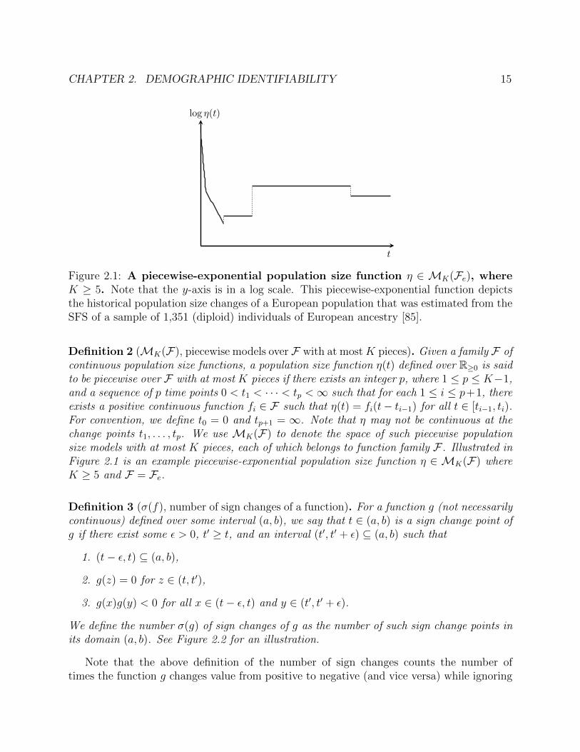
Figure 2.1: A piecewise-exponential population size function η ∈ MK(Fe), whereK ≥ 5. Note that the y-axis is in a log scale. This piecewise-exponential function depictsthe historical population size changes of a European population that was estimated from theSFS of a sample of 1,351 (diploid) individuals of European ancestry [85].
Definition 2 (MK(F), piecewise models over F with at mostK pieces). Given a family F ofcontinuous population size functions, a population size function η(t) defined over R≥0 is saidto be piecewise over F with at most K pieces if there exists an integer p, where 1 ≤ p ≤ K−1,and a sequence of p time points 0 < t1 < · · · < tp <∞ such that for each 1 ≤ i ≤ p+1, thereexists a positive continuous function fi ∈ F such that η(t) = fi(t− ti−1) for all t ∈ [ti−1, ti).For convention, we define t0 = 0 and tp+1 = ∞. Note that η may not be continuous at thechange points t1, . . . , tp. We use MK(F) to denote the space of such piecewise populationsize models with at most K pieces, each of which belongs to function family F . Illustrated inFigure 2.1 is an example piecewise-exponential population size function η ∈ MK(F) whereK ≥ 5 and F = Fe.
Definition 3 (σ(f), number of sign changes of a function). For a function g (not necessarilycontinuous) defined over some interval (a, b), we say that t ∈ (a, b) is a sign change point ofg if there exist some ε > 0, t′ ≥ t, and an interval (t′, t′ + ε) ⊆ (a, b) such that
1. (t− ε, t) ⊆ (a, b),
2. g(z) = 0 for z ∈ (t, t′),
3. g(x)g(y) < 0 for all x ∈ (t− ε, t) and y ∈ (t′, t′ + ε).
We define the number σ(g) of sign changes of g as the number of such sign change points inits domain (a, b). See Figure 2.2 for an illustration.
Note that the above definition of the number of sign changes counts the number oftimes the function g changes value from positive to negative (and vice versa) while ignoring

CHAPTER 2. DEMOGRAPHIC IDENTIFIABILITY 16
t1 t2 t3 t
g(t)
0
Figure 2.2: Illustration of the sign changes of a function. For the domain shown,σ(g) = 3 and the sign change points of g are denoted t1, t2, and t3.
intervals where it is identically zero. While the above definition is not restricted to piecewisecontinuous functions, we will restrict our attention to such functions for the remainder ofthis chapter.
Definition 4 (S (F) and S (MK(F)), sign change complexities). For a family F of con-tinuous population size functions, we define the sign change complexity S (F) as
S (F) = supf1,f2∈F ,a1,a2∈R≥0
σ(g)
∣∣∣∣∣∣∣g(τ) := f1(τ − a1)− f2(τ − a2) with domain
Dom(g) =
τ ∈ R≥0
∣∣∣∣∣ τ − a1 ∈ Dom(f1),
τ − a2 ∈ Dom(f2)
(2.13)
= supf1,f2∈F ,a∈R≥0
σ(g)
∣∣∣∣∣∣∣g(τ) := f1(τ)− f2(τ − a) with domain
Dom(g) =
τ ∈ R≥0
∣∣∣∣∣ τ ∈ Dom(f1),
τ − a ∈ Dom(f2)
, (2.14)
where fj are the time-rescaled versions of fj as defined in (2.3), and Dom(fj) = Rfj(R≥0)
is the domain of fj. Similarly, for the space MK(F) of piecewise population size modelswith at most K pieces over some function family F , we define the sign change complexityS (MK(F)) as
S (MK(F)) = supη1,η2∈MK(F)
σ(η1 − η2) , (2.15)
where, again, ηj are related to ηj as given in (2.3).
The following lemma gives a bound on the sign change complexity of a model with atmost K pieces in terms of the underlying family of population size functions for each piece.
Lemma 2. The sign change complexity of the space MK(F) of piecewise models with atmost K pieces in a function family F is bounded by the sign change complexity of F as
S (MK(F)) ≤ (2K − 2) + (2K − 1)S (F). (2.16)

CHAPTER 2. DEMOGRAPHIC IDENTIFIABILITY 17
Proof. Given a pair of piecewise population size functions η1, η2 ∈ MK(F), let η1 and η2
be their respective time-rescaled versions, defined by (2.3). Let 0 < t(1)1 < · · · < t
(1)p1 < ∞,
where 0 ≤ p1 ≤ K − 1, (respectively, 0 < t(2)1 < · · · < t
(2)p2 < ∞, where 0 ≤ p2 ≤ K − 1)
be the change points of the pieces of η1 (respectively, η2). We define t(1)0 = t
(2)0 = 0 and
t(1)p1+1 = t
(2)p2+1 = ∞. The change points of η1 are given by Rη1(t
(1)i ), where 1 ≤ i ≤ p1, while
the change points of η2 are given by Rη2(t(2)i ), where 1 ≤ i ≤ p2. Let 0 < τ1 < · · · < τp <∞
be the union of the change points of η1 and η2, where 0 ≤ p ≤ p1 + p2. For convention, letτ0 = 0 and τp+1 =∞.
Consider the piece (τi, τi+1) for 0 ≤ i ≤ p. Let I1 = (t(1)k , t
(1)k+1), where 0 ≤ k ≤ p1, and
I2 = (t(2)l , t
(2)l+1), where 0 ≤ l ≤ p2, be the pieces of the original population size functions
η1 and η2, respectively, such that (τi, τi+1) ⊆ Rη1(I1) and (τi, τi+1) ⊆ Rη2(I2). Since η1 ∈MK(F), there exists a function f1 ∈ F such that η1(t) = f1(t − t(1)
k ) for all t ∈ I1. Then,for all τ ∈ Rη1(I1),
η1(τ) = η1
(R−1η1
(τ))
= f1
(R−1η1
(τ)− t(1)k
)(2.17)
= f1
(Rf1
(R−1η1
(τ)− t(1)k
))(2.18)
= f1
(τ −Rη1(t
(1)k )). (2.19)
Similarly, there exists some function f2 ∈ F such that, for all τ ∈ Rη2(I2),
η2(τ) = f2
(τ −Rη2(t
(2)l )). (2.20)
Using (2.19) and (2.20), we see that the number of sign change points of η1− η2 in the piece
(τi, τi+1) is at most the number of sign change points of f1(τ −Rη1(t(1)k ))− f2(τ −Rη2(t
(2)l ))
for τ ∈ (τi, τi+1). Hence, by (2.14), it follows that within each piece (τi, τi+1) for 0 ≤ i ≤ p,η1 − η2 has at most S (F) sign change points. Also, the point τi+1 itself could be a signchange point in the interval between the last sign change point in piece (τi, τi+1) and thefirst sign change point in piece (τi+1, τi+2) where 0 ≤ i ≤ p − 1. These are all the possiblesign change points of η1 − η2. Hence,
σ(η1 − η2) ≤ p+ (p+ 1)S (F)
≤ (p1 + p2) + (p1 + p2 + 1)S (F)
≤ (2K − 2) + (2K − 1)S (F). (2.21)
Since (2.21) holds for all η1, η2 ∈MK(F), the lemma follows.
Note that the bound in Lemma 2 is tight for the family Fc of constant population sizes,for which S (Fc) = 0 and S (MK(Fc)) = 2K − 2.

CHAPTER 2. DEMOGRAPHIC IDENTIFIABILITY 18
2.3.3 Identifiability from the SFS
Our main results on identifiability will be proved using a generalization of Descartes’ rule ofsigns for polynomials:
Theorem 3 (Descartes’ rule of signs for polynomials). Consider a degree-n polynomialp(x) = a0 +a1x+ · · ·+anx
n with real-valued coefficients ai. The number of positive real roots(counted with multiplicity) of p is at most the number of sign changes between consecutivenon-zero terms in the sequence a0, a1, . . . , an.
The following theorem generalizes the above classic result to relate the number of signchanges of a piecewise-continuous function f to the number of roots of its Laplace transform:
Theorem 4 (Generalized Descartes’ rule of signs). Let f : R≥0 → R be a piecewise-continuous function which is not identically zero and with a finite number σ(f) of signchanges. Then, the function G(x) defined by
G(x) =
∫ ∞0
f(t)e−tx dt (2.22)
has at most σ(f) roots in R (counted with multiplicity).
Proof. The proof is by induction on the number of sign changes of f . If f has zero signchanges, then without loss of generality, f(t) ≥ 0 for t ∈ (0,∞) and f(t) > 0 for someinterval (a, b) ⊆ (0,∞). Hence, G(x) > 0 for all x, and the base case holds. Suppose f hasm+1 sign changes for some m ≥ 0. Let t0, . . . , tm be the set of sign change points of G(x).Note that G(x) and F (x) = et0xG(x) have the same real-valued roots (with multiplicity) sinceet0x > 0 for all x ∈ R. F ′(x) is given by
F ′(x) =d
dx
(∫ ∞0
f(t)e−(t−t0)x dt
)=
∫ ∞0
(t0 − t)f(t)e−(t−t0)x dt, (2.23)
where the interchange of the differential and integral operators in the second equality isjustified by the Leibniz integral rule because f is piecewise continuous over R≥0, and bothf(t)e−(t−t0)x and d
dx(f(t)e−(t−t0)x) are jointly continuous over (pi, pi+1) × (−∞,∞) for each
piece (pi, pi+1) over which f is continuous. Note that the set of sign change points of(t0 − t)f(t) is t1, . . . , tm. Hence (t0 − t)f(t) has only m sign changes. By the induc-tion hypothesis, F ′ has at most m real-valued roots. By Rolle’s theorem, the number ofreal-valued roots of F is at most one more than the number of real-valued roots of F ′.Hence, F has at most m+1 real-valued roots, implying that G has at most m+1 real-valuedroots.
The statement of Theorem 4 and its proof are adapted from Jameson [38, Lemma 4.5] forour setting. Using Theorem 4, we can prove the following main theorem on the identifiabilityof piecewise models when the pieces are from a family with finite sign change complexity:

CHAPTER 2. DEMOGRAPHIC IDENTIFIABILITY 19
Theorem 5. For a sample of size n, let c = (c2, . . . , cn), where cm = E[T(η)m,m], for 2 ≤
m ≤ n, defined in (2.5). If S (F) < ∞ and n ≥ 2K + (2K − 1)S (F), then no twodistinct models η1, η2 ∈ MK(F) can produce the same (c2, . . . , cn). In other words, forn ≥ 2K + (2K − 1)S (F), the map c :MK(F)→ Rn−1
+ is injective.
Proof. First, note that if S (F) < ∞, it follows from Lemma 2 that S (MK(F)) < ∞.Suppose there exist two distinct models η1, η2 ∈ MK(F) that produce exactly the same cmfor all 2 ≤ m ≤ n. From (2.7), we have that∫ ∞
0
(η1(τ)− η2(τ))e−(m2 )τdτ = 0 (2.24)
for 2 ≤ m ≤ n. If we define the function G(x) as
G(x) =
∫ ∞0
(η1(τ)− η2(τ))e−xτdτ, (2.25)
then from (2.24), we see that(m2
)is a root of G(x) for 2 ≤ m ≤ n, and hence, G has at least
n−1 roots. Applying Theorem 4 to the piecewise continuous function η1− η2, we see that Gcan have at most σ(η1 − η2) roots. Taking the supremum over all population size functionsη1 and η2 inMK(F), we see that G can have at most S (MK(F)) roots, and by Lemma 2,at most (2K−2)+(2K−1)S (F) roots. Hence, if n−1 > (2K−2)+(2K−1)S (F), we geta contradiction. This implies that if n ≥ 2K + (2K − 1)S (F), no two distinct populationsize functions in MK(F) can produce the same (c2, . . . , cn).
Using Theorem 5, it is simple to derive identifiability results for piecewise-defined popula-tion size models over several function families F that are of biological interest. In particular,we have the following result for the case of piecewise-constant models:
Corollary 6 (Identifiability of piecewise-constant population size models). For the spaceMK(Fc) of piecewise-constant population size models, the map c : MK(Fc) → Rn−1
+ isinjective if the sample size n ≥ 2K.
Proof. As remarked after Lemma 2, for the constant population size function family Fc,S (Fc) = 0. Hence, by Theorem 5, if n ≥ 2K, the map c :MK(Fc)→ Rn−1
+ is injective.
The bound in Corollary 6 on the sample size sufficient for identifying piecewise-constantpopulation models is actually tight, since MK(Fc) has 2K − 1 parameters in R+ and thereis no continuous injective function from R2K−1
+ to Rn−1+ if n < 2K. (This fact can be proved
in multiple ways, such as by the Borsuk-Ulam theorem or the Constant Rank theorem.) Wealso provide an alternate proof of Corollary 6 that does not explicitly rely on Theorem 5.This alternate proof is based on an argument from linear algebra, and it might be possibleto adapt this approach to develop an algebraic algorithm for inferring the parameters of apiecewise-constant population function from the set of expected first coalescence times cm.

CHAPTER 2. DEMOGRAPHIC IDENTIFIABILITY 20
An alternate proof of Corollary 6 based on linear algebra. Let n ≥ 2K, and suppose thereexist two distinct models η(1), η(2) ∈ MK(Fc) that produce exactly the same cm for all2 ≤ m ≤ n. Let η(1) and η(2) denote the time-rescaled versions of η(1) and η(2), respectively, asin (2.3). Since η(j) is piecewise-constant with at most K pieces, η(j) is also piecewise-constant
with the same number of pieces as η(j), and η(1) 6= η(2) implies η(1) 6= η(2). Therefore, ∆ :=η(1) − η(2) is a piecewise-constant function over [0,∞) with p pieces, where 1 ≤ p ≤ 2K − 1,
and ∆ is not identically zero. Let τ1 < · · · < τp−1 denote the change points of ∆, and define
τ0 = 0 and τp =∞. Suppose ∆(τ) = δi ∈ R for all τ ∈ [τi−1, τi), where 1 ≤ i ≤ p. Since η(1)
and η(2) produce the same cm for all 2 ≤ m ≤ n, we know that ∆ satisfies∫ ∞0
∆(τ)e−(m2 )τ dτ = 0, (2.26)
for all 2 ≤ m ≤ n. Substituting the definition of ∆ into (2.26) and multiplying by(m2
), we
obtain
p∑i=1
δi[e−(m
2 )τi−1 − e−(m2 )τi] = 0, (2.27)
for 2 ≤ m ≤ n. This defines a linear system Aδ = 0, where δ = (δ1, . . . , δp) and A = (ami)
is an (n− 1)× p matrix with ami := e−(m2 )τi−1 − e−(m
2 )τi for 2 ≤ m ≤ n and 1 ≤ i ≤ p.Let B = (bmi) be the (n− 1)× p matrix formed from A such that the ith column of B
is the sum of columns i, i + 1, . . . , p of A. Defining αi = e−τi−1 , note that bmi = α(m
2 )i for
2 ≤ m ≤ n and 1 ≤ i ≤ p. Now, consider the p × p submatrix C of B consisting of thefirst p rows of B. Since α1 > α2 > · · · > αp > 0, note that C is a generalized Vandermondematrix, which implies det(C) 6= 0 [22, Ch. XIII, §8]. Hence, rank(B) = p. The rank ofA is invariant under elementary column operations, and therefore rank(A) = rank(B) = p.Therefore, the kernel of A is trivial, and the only solution to (2.27) is δ1 = δ2 = · · · = δp = 0,
which contradicts our assumption that ∆ = η(1) − η(2) 6≡ 0.
Another class of models often assumed in population genetic analyses are piecewise-exponential functions, for which we have the following result:
Corollary 7 (Identifiability of piecewise-exponential population size models). For the spaceMK(Fe) of piecewise-exponential population size models, the map c : MK(Fe) → Rn−1
+ isinjective if the sample size n ≥ 4K − 1.
Proof. Let f1, f2 ∈ Fe be given by
f1(t) = ν1 exp(β1t), (2.28)
f2(t) = ν2 exp(β2t), (2.29)

CHAPTER 2. DEMOGRAPHIC IDENTIFIABILITY 21
where t ∈ R≥0, ν1, ν2 ∈ R+ and β1, β2 ∈ R. Then, for i = 1, 2, the time-rescaled function fiis given by
fi(τ) =νi
1− νiβiτ, (2.30)
for τ ∈ Dom(fi) = Rfi(R≥0) = [0, 1νiβi
). From (2.30), it can be seen that f1 and f2 arecontinuous in their domains. Furthermore, for any given a ∈ R≥0, there is at most one
τ , where τ ∈ Dom(f1) and τ − a ∈ Dom(f2), such that g(τ) := f1(τ) − f2(τ − a) = 0,implying σ(g) ≤ 1. By the definition of sign change complexity in (2.14), it then followsthat S (Fe) ≤ 1 for the exponential population family Fe. Hence, applying Theorem 5, weconclude that n ≥ 4K − 1 suffices for the map c :MK(Fe)→ Rn−1
+ to be injective.
For the identifiability of piecewise population size models from the SFS data, we firstnote the following lemma:
Lemma 8. Consider a piecewise population size function η ∈ MK(F). Consider a sample
of size n ≥ 2K + (2K − 1)S (F) and suppose the function η produces E[T(η)m,m] = cm for
2 ≤ m ≤ n. Then, for every fixed κ ∈ R+, there exists a unique piecewise population size
function ζ ∈MK(F) with E[T(ζ)m,m] = κcm for 2 ≤ m ≤ n. Furthermore, this population size
function ζ is given by ζ(t) = κη(t/κ).
Proof. For the population size function ζ(t) defined by ζ(t) = κη(t/κ), note that Rζ(t) isgiven by
Rζ(t) =
∫ t
0
1
ζ(x)dx =
∫ t
0
1
κη(x/κ)dx =
∫ t/κ
0
1
η(x)dx = Rη(t/κ).
E[T(ζ)m,m] is then given by
E[T (ζ)m,m] =
∫ ∞0
exp
[−(m
2
)Rη
(t
κ
)]dt (2.31)
= κ
∫ ∞0
exp
[−(m
2
)Rη(t)
]dt (2.32)
= κE[T (η)m,m]. (2.33)
Since n ≥ 2K + (2K − 1)S (F), by Theorem 5, ζ is the unique population size function in
MK(F) with E[T(ζ)m,m] = κcm for 2 ≤ m ≤ n.
Given two models η, ζ ∈MK , we say that η and ζ are equivalent, and write η ∼ ζ, if theyare related by a rescaling of change points and population sizes as described in Lemma 8.Then, combining Lemma 1, Theorem 5, and Lemma 8, we obtain the following theorem:
Theorem 9. If S (F) < ∞ and n ≥ 2K + (2K − 1)S (F), then, for each expected SFS(ξn,1, . . . , ξn,n−1), there exists a unique equivalence class [η] of models inMK(F)/∼ consistentwith (ξn,1, . . . , ξn,n−1).

CHAPTER 2. DEMOGRAPHIC IDENTIFIABILITY 22
2.3.4 Extension to the folded frequency spectrum
To generate the SFS from genomic sequence data, one needs to know the identities of theancestral and mutant alleles at each site. To avoid this problem, a commonly employedstrategy in population genetic inference involves “folding” the SFS. More precisely, for asample of size n, the i-th entry of the folded SFS χ = (χn,1, . . . , χbn/2c) is defined by
χn,i =ξn,i + ξn,n−i1 + δi,n−i
, (2.34)
where 1 ≤ i ≤ bn/2c. In particular, χn,i is the proportion of polymorphic sites that have icopies of the minor allele. For any sample size n, since χ is a vector of approximately halfthe dimension as ξ, we might expect to require roughly twice as many samples to recover thedemographic model from χ compared to ξ. This is indeed the case. Given the folded SFS χ,the following theorem establishes a sufficiency condition on the sample size for identifyingdemographic models in MK(F):
Theorem 10. If S (F) < ∞ and n ≥ 2(2K − 1)(1 + S (F)), then, for each expectedfolded SFS χ = (χn,1, . . . , χn,bn/2c), there exists a unique equivalence class [η] of models inMK(F)/∼ consistent with χ.
To prove Theorem 10, we first need a lemma that characterizes a certain symmetryproperty of the invertible matrix that relates the genealogical quantities γ and c introducedin the proof of Lemma 1.
Lemma 11. For a sample of size n, let W be the (n − 1) × (n − 1) invertible matrix suchthat γn,b =
∑nm=2Wb,mcm, where γn,b is the total expected branch length subtending b leaves
and cm = E[T(η)m,m]. Then, for every b and m, where 1 ≤ b ≤ n− 1 and 2 ≤ m ≤ n, we have
the following identities:
Wb,m +Wn−b,m = 0, if m is odd, (2.35)
Wb,m −Wn−b,m = 0, if m is even. (2.36)
Proof. From the proof of Lemma 1, it can be seen that the matrix W is the product of3 matrices whose entries are explicitly given combinatorial expressions. However, usingZeilberger’s algorithm [66], Polanksi and Kimmel [69, Equations 13–15] also derived thefollowing recurrence relation for the entries of W :
Wb,2 =6
(n+ 1),
Wb,3 = 30(n− 2b)
(n+ 1)(n+ 2),
Wb,m+2 = f(n,m)Wb,m + g(n,m)(n− 2b)Wb,m+1, (2.37)

CHAPTER 2. DEMOGRAPHIC IDENTIFIABILITY 23
where f(n,m) and g(n,m) are rational functions of n and m given by
f(n,m) = −(1 +m)(3 + 2m)(n−m)
m(2m− 1)(n+m+ 1),
g(n,m) =(3 + 2m)
m(n+m+ 1).
It will be easy to prove our lemma by induction on m using (2.37). The base cases are easyto check:
Wb,2 −Wn−b,2 = 0,
Wb,3 +Wn−b,3 = 30(n− 2b) + (n− 2(n− b))
(n+ 1)(n+ 2)= 0.
Using (2.37), we see that if m is odd,
Wb,m+2 +Wn−b,m+2
= f(n,m)(Wb,m +Wn−b,m)
+ g(n,m)(n− 2b)Wb,m+1 + [n− 2(n− b)]Wn−b,m+1= f(n,m)(Wb,m +Wn−b,m) + g(n,m)(n− 2b)(Wb,m+1 −Wn−b,m+1)
= 0,
where the last equality follows from the induction hypothesis which implies Wb,m+Wn−b,m =0 and Wb,m+1 −Wn−b,m+1 = 0. Similarly, if m is even,
Wb,m+2 −Wn−b,m+2
= f(n,m)(Wb,m −Wn−b,m)
+ g(n,m)(n− 2b)Wb,m+1 − [n− 2(n− b)]Wn−b,m+1= f(n,m)(Wb,m −Wn−b,m) + g(n,m)(n− 2b)(Wb,m+1 +Wn−b,m+1)
= 0,
where again the last equality follows from the induction hypothesis.
Proof of Theorem 10. For a sample of size n in the coalescent, let γn,b be the total expectedbranch length subtending b leaves, for 1 ≤ b ≤ n− 1. Then, there exists a positive constantκ such that
γn,d + γn,n−d1 + δd,n−d
= κχn,d, (2.38)
for all 1 ≤ d ≤ bn/2c. Let fn,d =γn,d+γn,n−d
1+δd,n−d. The relationship between f = (fn,1, . . . , fn,bn/2c)
and γ = (γn,1, . . . , γn,n−1) can be described by the linear equation
f = Zγ, (2.39)

CHAPTER 2. DEMOGRAPHIC IDENTIFIABILITY 24
where Z is an bn/2c × (n− 1) matrix with entries given by
Zdj =
1, if j = d or j = n− d,0, otherwise,
(2.40)
for 1 ≤ d ≤ bn/2c and 1 ≤ j ≤ n− 1. Hence, dim(ker(Z)) = b(n−1)/2c.From Lemma 1, we know that γ and c = (c2, . . . , cn) are related as γ = Wc, where
W = (Wb,m) is an (n− 1)× (n− 1) invertible matrix, where 1 ≤ b ≤ n− 1 and 2 ≤ m ≤ n.Hence,
f = Y c, (2.41)
where Y := ZW . Since Yb,m = Wb,m + Wn−b,m, we know from Lemma 11 that Yb,m = 0for all odd values of m. Therefore, every other column of the matrix Y is zero. Thisimplies that span(e3, e5, . . . , en−1n even) ⊆ ker(Y ), where ei is an (n − 1)-dimensionalunit vector defined as ei = (ei,2, . . . , ei,n), with ei,i = 1 and ei,j = 0 for i 6= j. Note thatn − 1n even = 2b(n−1)/2c + 1 and dim(span(e3, e5, . . . , e2b(n−1)/2c+1)) = b(n−1)/2c. Now,since W is invertible, dim(ker(Y )) = dim(ker(ZW )) = dim(ker(Z)) = b(n−1)/2c. Therefore,
ker(Y ) = span(e3, e5, . . . , e2b(n−1)/2c+1
). (2.42)
Suppose there exist two distinct models η1, η2 ∈ MK(F) that produce the same foldedSFS f . Let c(1) and c(2) be the vector of genealogical quantities for models η1 and η2
respectively, where c(1)m = E[T
(η1)m,m] and c
(2)m = E[T
(η2)m,m], 2 ≤ m ≤ n. From (2.41), we know
that c(1) − c(2) ∈ ker(Y ). Using (2.42), c(1)m − c(2)
m can be written as
c(1)m − c(2)
m =
b(n−1)/2c∑l=1
αle2l+1,m, (2.43)
for some αl ∈ R. Since eij = 0 for i 6= j, (2.43) implies that c(1)m − c(2)
m = 0 for all even valuesof m, where 2 ≤ m ≤ n. Now applying a similar argument as in the proof of Theorem 5 toc
(1)m − c(2)
m for even values of m, we conclude that if d(n−1)/2e > (2K − 2) + (2K − 1)S (F),then no two distinct models η1, η2 ∈ MK(F) can produce the same f . This implies that asample size n ≥ 2(2K − 1)(1 + S (F)) suffices for identifying the population size function inMK(F) from the folded SFS f , and the conclusion of the theorem follows from (2.38) andLemma 8.
2.4 The counterexample of Myers et al.
Myers et al. [61] provided an explicit counterexample to the identifiability of population sizemodels from the allelic frequency spectrum. In our notation, they provided two time-rescaledpopulation size functions η1 and η2 given by
η1(τ) = N, (2.44)

CHAPTER 2. DEMOGRAPHIC IDENTIFIABILITY 25
η2(τ) = N(1− 9F (τ)), (2.45)
where N is an arbitrary positive constant, and the function F is given by the convolution
F (τ) =
∫ τ
0
f0(τ − u)f1(u)du, (2.46)
where f0 and f1 are given by
f0(τ) = exp(−1/τ 2), (2.47)
f1(τ) =cos(π2/τ) exp(−τ/8)√
τ. (2.48)
Both functions f1 and F have increasingly frequent oscillations as τ ↓ 0 so that σ(η1− η2) =σ(F ) =∞. This is why Theorem 5 does not apply to this example. Indeed, by an argumentusing the Laplace transforms of f1 and F , Myers et al. showed that the function G(x) definedin (2.22) in terms of F has roots at −
(m2
)for each m ≥ 2.
2.5 Discussion
In human genetics, several large-sample datasets have recently become available, with samplesizes on the order of several thousands to tens of thousands of individuals [1, 12, 19, 62, 85].The patterns of polymorphism observed in these datasets deviate significantly from thatexpected under a constant population size, and there has been much interest to infer recentand ancient human demographic changes that might explain these deviations [23, 48, 51].Clearly, model identifiability is an important prerequisite for such statistical inference prob-lems. In this chapter, we have obtained mathematically rigorous identifiability results fordemographic inference by showing that piecewise-defined population size functions over awide class of function families are completely determined by the SFS, provided that thesample is sufficiently large. Furthermore, we have provided explicit bounds on the samplesizes that are sufficient for identifying such piecewise population size functions. These boundsdepend on the number of pieces and the functional type of each piece. For piecewise-constantpopulation size models, which have been extensively applied in demographic inference stud-ies, our bounds are tight. We have also given analogous results for identifiability from thefolded SFS, a variant of the SFS that is oblivious to the identities of the ancestral and mutantalleles.
Our work suggests several interesting avenues for future research. In our work, we exam-ined the identifiability of demography from the expected SFS data. However, if one were touse the complete sequence data or other summary statistics such as the length distributionof shared haplotype tracts, it might be possible to uniquely identify the demography usingeven smaller sample sizes than that needed when using only the SFS. Indeed, several demo-graphic inference methods have been developed to infer historical population size changes

CHAPTER 2. DEMOGRAPHIC IDENTIFIABILITY 26
from such data using anywhere from a pair of genomic sequences [34, 48, 64] to tens of suchsequences [79], and it is important to theoretically characterize the power and limitations ofboth the data and the inference methods.
Another interesting direction for exploration is to understand the extent to which ancientdemographic events can be inferred from the SFS in practice. The population size changessufficiently far back in the past are likely to have only a marginal effect on the SFS since theindividuals in the sample are highly likely to have found a common ancestor by such ancienttimes. Our identifiability results apply in the limit that the genome length is infinite, whichallows one to estimate the entries of the expected SFS exactly. However, a finite lengthgenome does not permit exact estimation of the SFS, and it might be difficult to resolve veryancient demographic events. Another question related to this issue is understanding thesensitivity of the SFS to perturbations in the demographic parameters. This is importantfor quantifying the extent to which errors in estimating the expected SFS from data affectthe parameter estimates in inferred demographic models.
It would also be interesting to consider the possibility of developing an algebraic algo-rithm for demographic inference that closely mimics the linear algebraic proof of Corollary 6provided in Section 2.3.3. For example, using a sample of size K + 1, one could consider in-ferring a piecewise-constant model with K pieces, with one piece for each of the most recentK − 1 generations and another piece for the population size further back in time. (Here weare considering a restricted class of piecewise-constant population size functions with fixedchange points, so the minimum sample size needed for distinguishing such models using theSFS is K + 1 rather than 2K.) Such an algebraic algorithm could provide a more principledway of inferring demographic parameters, compared to existing inference methods that relyon optimization procedures which lack theoretical guarantees for functions with multiplelocal optima.

27
Chapter 3
Inference of the population sizefunction from SFS data
3.1 Overview
Motivated by recent large-sample exome-sequencing studies [62,85] which have greater powerto capture rare variants than previous analyses involving small sample sizes [23, 31], in thischapter, we study the problem of efficiently inferring population size changes and mutationrates in a large randomly mating population using the SFS of a sample of individuals atmultiple loci.
There have been several previous approaches to this problem. Coventry et al. [12] de-veloped a method based on coalescent tree simulations to infer population size changes andper-locus mutation rates, and applied this to exome-sequencing data from approximately10,000 individuals at 2 genes. Using coalescent simulations to empirically estimate the ex-pected SFS under a given demographic model, Coventry et al. compute a likelihood functionfor the demographic model by comparing the expected and observed SFS. Nelson et al. [62]have also applied this method to a dataset of 11,000 individuals of European ancestry (CEU)sequenced at 188 genes to infer a recent epoch of exponential population growth. Excoffier etal. [16] have developed a software package that uses coalescent tree simulations to estimatethe expected joint SFS of multiple subpopulations for inferring potentially very complex de-mographic scenarios. This problem has also been approached from the diffusion perspective.Gutenkunst et al. [31] used numerical schemes to solve the partial differential equation forthe density of segregating sites at a given derived allele frequency, while Lukic et al. [52]approximated the solutions to these equations using spectral methods.
Similar to the inference methods of Coventry et al. and Excoffier et al., we also work inthe coalescent framework rather than in the diffusion setting. However, our method differsfrom existing methods in several ways. First, our method is based on exact computation anddoes not require any Monte-Carlo coalescent simulations. We use an efficient algorithmicadaption of the analytic theory of the SFS for deterministically varying population size

CHAPTER 3. DEMOGRAPHIC INFERENCE 28
models that was developed by Polanski et al. [68] and Polanski and Kimmel [69]. As aresult, our method is extremely efficient compared to simulation-based approaches, allowingus to more thoroughly search the space of demographic models of interest. Second, ourmethod uses the Poisson Random Field (PRF) approximation proposed by Sawyer andHartl [76]. Under this approximation, all the segregating sites in a single locus are assumedto be far enough apart to be completely unlinked. This is also the same approximation madeby the numerical and spectral methods for demographic inference under the Wright-Fisherdiffusion process [31,52]. At the other extreme, the method of Coventry et al. for populationsize inference assumes that all the segregating sites in a locus are completely linked. Boththese model simplifications, which assume that a locus is a collection of completely linkedor completely unlinked sites, are biologically unrealistic. However, as we demonstrate inour results on simulated data, our method can recover demographic parameters accuratelyeven when the data is generated under realistic recombination rates. Third, working in thePRF model also confers our method a significant computational benefit. Under the PRFmodel, we can write down efficiently computable expressions for the the maximum likelihoodestimate of the mutation rates at each locus. This contrasts with the method of Coventry etal. where a line search has to be performed over the mutation rates due to the Monte-Carlointegration involved. Fourth, under the PRF model, the maximum likelihood estimate forthe demographic model has a nice mathematical interpretation in that it is the demographicmodel which minimizes the KL divergence of the expected SFS from the observed SFS.Our method also has advantages over the diffusion-based methods of Gutenkunst et al. [31]and Lukic et al. [52]. Since we are working in the coalescent framework, the running timeof our method is independent of the population size and our computations are exact up tonumerical precision. On the other hand, the method of Gutenkunst et al. discretizes the allelefrequency space, while the spectral method of Lukic et al. [52] has to choose the numberof basis elements for the representation of the Wright-Fisher transition density function.Finally, since our method is based on a likelihood function that is computed exactly, we cantake advantage of automatic differentiation [24] to compute numerically exact gradients of thelikelihood function, and thus take advantage of gradient-based algorithms for optimizationover the space of demographic parameters.
As we have seen in previous chapters, a result of Myers et al. [61] shows that it isinformation-theoretically not possible to uniquely recover general population size functionsfrom the SFS. However, as we proved in Chapter 2, if we assume that the true populationsize function is piecewise-constant or piecewise-exponential, then the expected SFS of alarge enough sample uniquely determines the piecewise population size function. Takingadvantage of this identifiability result, we perform inference under the assumption that thetrue population size function is piecewise-exponential (which also allows for constant pieces).
The rest of this chapter is organized as follows. We introduce the relevant notation inSection 3.2, and describe some of the details of our method in Section 3.3. The details of thetheory and computation in our method are given in 3.3.2. In Section 3.4, we demonstrateour method on simulated data using biologically reasonable parameters.

CHAPTER 3. DEMOGRAPHIC INFERENCE 29
3.2 Notation
The data we wish to analyze, denoted by D, consists of the unnormalized SFS for n haploid(or n/2 diploid) individuals at each of G loci located sufficiently far apart in the genome.
The unnormalized SFS at locus g is a vector o(g) = (o(g)1 , . . . , o
(g)n−1), where o
(g)i is the number
(rather than the probability) of segregating sites at locus g which have i copies of the mutant
allele among the n alleles at that site. For notational convenience, let o(g) =∑n
i=1 o(g)i be
the total number of segregating sites in the sample at locus g. We are also given the lengthm(g) of each locus g. Given the data D, our goal is to infer the haploid piecewise-exponentialeffective population size function N(t) and the per-base locus specific mutation rates µ(g).Note that in this chapter, we work with the population size functions N(t) in physical unitsrather than coalescent rate functions η(t) used in Chapter 2. The conversion from η(t) toN(t) can be done if we have knowledge of, for example, the ancestral population size or themutation rate at some locus in physical units (i.e. per generation). We will use Φ to denotethe parameterization of the population size function in the family of piecewise-exponentialmodels we consider in this work. While we state our method assuming we have access tothe SFS, we can just as easily work with the folded SFS if the identities of the ancestral andmutant alleles are uncertain.
3.3 Method
Let us first restrict attention to a single locus g. For a locus with length m bases and per-base per-generation mutation rate µ, let θ denote the population-scaled mutation rate forthe whole locus. Specifically, in the infinite-sites model, θ is given by,
θ = 4Nrmµ,
where Nr denotes a reference population size which is used as a scaling parameter. Wewish to compute the probability of the observed frequency spectrum o at locus g under theinfinite-sites model. If all the sites in the locus were completely linked and the n individualsin the sample are related according to the coalescent tree T , then the probability of observingthe frequency spectrum o is given by,
P(o | T,Φ, θ) =n−1∏i=1
exp
(−θ
2τn,i(T )
) ( θ2τn,i(T )
)oioi!
, (3.1)
where τn,i(T ) is the sum of the lengths of branches in the coalescent tree T which subtendidescendant leaves. The explanation for (3.1) is as follows. In the infinite-sites model,mutations are dropped on the coalescent tree according to a Poisson process with rate θ/2,and every mutation generates a new segregating site. A mutation creates a segregating sitewith i mutant alleles if it occurs on a branch that subtends i descendants. To avoid unwieldynotation, we drop the dependence on the tree T for the branch lengths τn,i(T ). To compute

CHAPTER 3. DEMOGRAPHIC INFERENCE 30
the probability of the observed frequency spectrum o, we have to integrate (3.1) over thedistribution f(T | Φ) of coalescent trees T in the space of coalescent trees Tn over n leaves.Abusing notation, this can be written as
P(o | Φ, θ) =
∫Tn
P(o | T,Φ, θ)f(T | Φ) dT
=
∫Tn
[n−1∏i=1
exp
(−θ
2τn,i
) ( θ2τn,i)oi
oi!
]f(T | Φ) dT
=
∫Tn
[n−1∏i=1
(θ2τn,i)oi
oi!
]exp
(−θ
2Ln
)f(T | Φ) dT
P(o | Φ, θ) =
∫Tn
(o
o1, . . . , on
)[n−1∏i=1
(τn,iLn
)oi]exp
(−θ
2Ln
) ( θ2Ln)o
o!f(T | Φ) dT. (3.2)
In (3.2), Ln is the total branch length of the tree T on n haploid individuals. It is notknown how to efficiently and exactly compute (3.2), even when Φ represents the constantpopulation size model. Coventry et al. [12] and Nelson et al. [62] approximate the integral in(3.2) by drawing random coalescent trees under the demographic model Φ. In order to findthe MLE for θ, they repeat this Monte-Carlo integration for each value of θ in some grid.
3.3.1 Poisson Random Field approximation
In our method, we use the Poisson Random Field (PRF) approximation of Sawyer andHartl [76] which assumes that all the sites in a given locus are completely unlinked, andhence the underlying coalescent tree at each site is independent. Under this assumption, theprobability of the frequency spectrum o is given by,
P(o | Φ, θ) =n−1∏i=1
(θ2E[τn,i]
)oi!
oi
exp
(−θ
2E[Ln]
)
= C
n−1∏i=1
(θ
2E[τn,i]
)oiexp
(−θ
2E[Ln]
)(3.3)
where the expectation in (3.3) is taken over the distribution on coalescent trees T over nleaves, and C =
∏n−1i=1
1oi!
is a data-dependent constant that can be ignored for maximumlikelihood estimation. Hence, under the PRF approximation, the problem of computingthe likelihood in (3.3) reduces to that of computing the quantities E[τn,i] and E[Ln] underthe given demographic model Φ. Using the theory of the SFS for variable population sizesdeveloped by Polanski et al. [68] and Polanski and Kimmel [69], we can develop an efficientalgorithm to numerically stably and exactly compute E[τn,i] and E[Ln] for a wide class ofpopulation size functions N(t). In our work, we consider the family of piecewise-exponential

CHAPTER 3. DEMOGRAPHIC INFERENCE 31
functions. The details of computing E[τn,i] and E[Ln] for such a class of population sizefunctions is given in Section 3.3.2. Taking logarithms on both sides in (3.3), we get thefollowing log-likelihood for the demographic model Φ and mutation rate θ at this locus,
L(Φ, θ) = logP(o | Φ, θ) =n−1∑i=1
oi (logE[τn,i] + log θ)− θ
2E[Ln] + constant(o). (3.4)
Assuming the loci are all completely unlinked, the log-likelihood for one locus given in (3.4)can be summed across all loci g to get a log-likelihood for the entire dataset D,
L(Φ, θ(g)Gg=1) = logP(D | Φ, θ(g)Gg=1)
=G∑g=1
[n−1∑i=1
o(g)i
(logE[τn,i] + log θ(g)
)− θ(g)
2E[Ln]
]+ constant(o). (3.5)
It is easy to see that L is a concave function of the mutation rates θ(g), since the Hessian Hof L with respect to θ(g) is given by,
Hg,h =∂2L
∂θ(g)∂θ(h)= −δg,h
1
θ(g)2
n−1∑i=1
o(g)i , (3.6)
showing that H is negative definite. Hence, the mutation rates of the loci that maximize Lare the solutions of,
0 =∂L∂θ(g)
=1
θ(g)
n−1∑i=1
o(g)i −
1
2E[Ln], (3.7)
yielding the maximum likelihood estimate for the mutation rate θ(g) at locus g given thedemographic model,
θ(g) =2∑n−1
i=1 o(g)i
E[Ln]. (3.8)
Note that for a constant population size, (3.8) is the same as Watterson’s estimator θ(g)W for
the mutation rate [92],
θ(g)W =
∑n−1i=1 o
(g)i∑n−1
i=11i
,
since for a constant population size, E[Ln] =∑n−1
i=11i. Substituting the MLE for θ(g) in (3.8)
into (3.5), we have the log-likelihood with the optimal mutation rates,
L(Φ) =n−1∑i=1
[(G∑g=1
o(g)i
)log
(E[τn,i]
E[Ln]
)]+ constant(o). (3.9)

CHAPTER 3. DEMOGRAPHIC INFERENCE 32
If we define the n-dimensional discrete probability distributions o and τn by
ok =
∑Gg=1 o
(g)k∑n−1
i=1
∑Gg=1 o
(g)i
,
and
τn,k =E[τn,k]
E[Ln],
where 1 ≤ k ≤ n − 1, then we see that the demographic model Φ∗ that is the MLE of thelikelihood function L(Φ) in (3.9) is given by,
Φ∗ = arg maxΦ
L(Φ)
= arg minΦ
KL(o || τ2n), (3.10)
where KL(P || Q) denotes the KL divergence of distribution Q from P . Hence, giventhe demographic model, we can efficiently infer the optimal mutation rate at each locusindependently according to (3.8) and compute the log-likelihood using (3.9). We can alsocompute the gradient of L(Φ) with respect to Φ using automatic differentiation [24], andsearch over the space of demographic models using a gradient-based optimization method.
3.3.2 Computing the expected SFS under a variable populationsize
In this section, we describe the details of computing the quantities E[τn,i] and E[Ln], theexpected branch length subtending i leaves and the expected total branch length respectively,when a coalescent tree is drawn over n individuals according to Kingman’s coalescent withdemographic model Φ.
Polanski and Kimmel [69] showed that τn,i and E[Ln] can be computed efficiently andnumerically stably using the relations,
E[τn,i] =n∑
m=2
Wn,i,mcm, (3.11)
E[Ln] =n∑
m=2
Vn,mcm, (3.12)
where the coefficients Wn,i,m and Vn,m are efficiently computable by dynamic programming[69, Equations 12–15], the coefficients cm are given by the integral,
cm =
∫ ∞0
exp
[−(m
2
)R(t)
]dt, (3.13)

CHAPTER 3. DEMOGRAPHIC INFERENCE 33
and R(t) is a time-rescaling function for the coalescent process, given by the expression,
R(t) =
∫ t
0
Nr
N(τ)dτ. (3.14)
In this work, we consider the class of piecewise-exponential population size functions. Anypopulation size function in this family of functions can be described by M + 1 time points,0 = t0 < t1 < · · · < tM = ∞, where the effective population size in time interval [ti, ti+1),0 ≤ i ≤ M − 1, is given by N(t) = N(ti) exp(−βi+1(t − ti)). The times ti are in units ofNr generations. In the piece corresponding to time interval [ti−1, ti), exponential populationgrowth (decline) is encoded by βi > 0 (βi < 0), while βi = 0 represents a constant population.For this family of population models, we can compute the integrals in (3.13) as follows. Fort ∈ [ti, ti+1), 0 ≤ i ≤M − 1,
R(t)−R(ti) = 1[βi+1 = 0]Nr
N(ti)(t− ti) + 1[βi+1 6= 0]
1
βi+1
Nr
N(ti)(exp(βi+1(t− ti))− 1)
(3.15)
cm =M∑i=1
∫ ti
ti−1
exp
(−(m
2
)R(t)
)dt
=M∑i=1
exp
(−(m
2
)R(ti−1)
)∫ ti
ti−1
exp
(−(m
2
)(R(t)−R(ti−1))
)dt
=M∑i=1
exp
(−(m
2
)R(ti−1)
)1[βi = 0]
∫ ti
ti−1
exp
(−(m
2
)Nr
N(ti−1)(t− ti−1)
)dt +
1[βi 6= 0]
∫ ti
ti−1
exp
(−(m
2
)1
βi
Nr
N(ti−1)(exp(βi(t− ti−1))− 1)
)
cm =M∑i=1
1[βi = 0]1(m2
)N(ti−1)
Nr
exp
(−(m
2
)R(ti−1)
)− exp
(−(m
2
)R(ti)
)
+M∑i=1
1[βi 6= 0]1
βiexp
(−(m
2
)R(ti−1)
)exp
(1
βi
(m
2
)Nr
N(ti−1)
)×
Ei
(−(m
2
)Nr
N(ti−1)
exp(βi(ti − ti−1))
βi
)− Ei
(−(m
2
)Nr
N(ti−1)
1
βi
),
(3.16)
where Ei(x) is the exponential integral special function, given by,
Ei(x) = −∫ ∞−x
e−t
tdt. (3.17)

CHAPTER 3. DEMOGRAPHIC INFERENCE 34
Equation (3.16) can be further simplified to get
cm =M∑i=1
1[βi = 0]1(m2
)N(ti−1)
Nr
exp
(−(m
2
)R(ti−1)
)− exp
(−(m
2
)R(ti)
)+
M∑i=1
1[βi 6= 0]1
βi
exp
(−(m
2
)R(ti)
)exp
((m
2
)Nr
N(ti−1)
exp(βi(ti − ti−1))
βi
)×
Ei
(−(m
2
)Nr
N(ti−1)
exp(βi(ti − ti−1))
βi
)− exp
(−(m
2
)R(ti−1)
)exp
((m
2
)Nr
N(ti−1)
1
βi
)Ei
(−(m
2
)Nr
N(ti−1)
1
βi
),
(3.18)
We evaluate terms of the form exp(x)Ei(−x) that appear in (3.18) for large values of xusing the following asymptotic expansion,
exp(x)Ei(−x) = −1
x
∞∑k=0
(−1)kk!
xk. (3.19)
For the results in Section 3.4, we truncated the divergent expansion (3.19) after 10 terms forx ≥ 45.
3.4 Results
To test the performance of our method, we simulated data under the following demographicscenarios:
• Scenario 1 – One epoch of exponential growth, with several different parameter valuesfor the per-generation growth rate r1 and the duration of growth t1. For all of thesechoices, the population expansion factor, (1 + r1)t1 , was fixed at approximately 512,which was also roughly equal to the MLE for the population expansion factor in theCEU subpopulation inferred by Nelson et al. [62]. The ancestral population size priorto the onset of exponential growth was fixed at 7700 diploids following the estimate ofSchaffner et al. [77] for the CEU subpopulation.
• Scenario 2 – Two epochs of exponential growth, the more ancient of which lasts fort2 = 300 generations with a growth rate of r2 = 1% per generation, and a more recentepoch of rapid growth lasting t1 = 100 generations with a growth rate of r1 = 4%per generation. This model also has two population bottlenecks inferred by Keinan etal. [40]. The ancestral population size was fixed at 104 diploids.

CHAPTER 3. DEMOGRAPHIC INFERENCE 35
The population size functions, N(t), for both these scenarios are shown in Figure 3.1. Foreach scenario, we generated 100 simulated datasets using Hudson’s ms program [36] with asample size of 10,000 diploid individuals. For Scenario 1, we simulated 200 loci of length10kb, with the mutation rates at each locus randomly chosen from the range 1.1 × 10⁻⁸ to3.8×10−8 per bp per generation, and then held fixed across all the simulated datasets. Theseare also the range of mutation rates estimated from family trios by Conrad et al. [11]. ForScenario 2, we simulated 1000 loci of length 1kb, each with mutation rate 2.5× 10⁻⁸ per bpper generation. For both scenarios, we used a realistic recombination rate of 10−8 per bpper generation within each locus.
Figure 3.2 shows the inferred values of the duration and rate of exponential growth forthe various values of r1 and t1 in Scenario 1, while Figure 3.3 shows the inferred values of theduration and growth rates for each of the two epochs in Scenario 2. The inferred mutationrates for one setting of parameter values for Scenario 1, and for Scenario 2 are shown inFigures 3.4 and 3.5 respectively. As can be seen from Figures 3.2 and 3.4, our method is ableto accurately infer the growth parameters and per-locus mutation rate at each of the loci inScenario 1. While there is more uncertainty in the inference of the growth parameters andmutation rates in Scenario 2, the estimates appear unbiased. With larger sample sizes ormore segregating sites, this uncertainty in the parameter estimates is expected to decrease.
For all these simulation results, we combined the counts of those segregating sites whichfell in the top 90% of segregating sites ordered by minor allele frequency. To search over thespace of demographic models, we used the optimization program IPOPT [88] with gradientscomputed using the automatic differentiation library ADOL [91]. Using the binning schemementioned above, the optimization over the two parameters in Scenario 1 takes about 10CPU seconds, and that over the four parameters in Scenario 2 takes about a CPU minute.

CHAPTER 3. DEMOGRAPHIC INFERENCE 36
0 200 400 600 800 1000 1200 1400 1600Time t, in generations
103
104
105
106
107
Popu
lati
onsi
zeN
(t)
1 epoch of recent population expansion
t1 = 100, r1 = 6.4%
t1 = 200, r1 = 3.2%
t1 = 300, r1 = 2.1%
t1 = 400, r1 = 1.6%
t1 = 500, r1 = 1.3%
t1 = 600, r1 = 1.0%
t1 = 700, r1 = 0.9%
(a)
0 1000 2000 3000 4000 5000Time t, in generations
102
103
104
105
106
107
Popu
lati
onsi
zeN
(t)
2 epochs of recent population expansion
(b)
Figure 3.1: Population size N(t) as a function of time (number of generations ago)for (a) several choices of t1 and r1 in Scenario 1 and (b) Scenario 2. The presenttime corresponds to t = 0.

CHAPTER 3. DEMOGRAPHIC INFERENCE 37
100 200 300 400 500 600 700True t1 (in generations)
0
100
200
300
400
500
600
700
800In
ferr
edt 1
(in
gene
rati
ons)
(a)
6.4 3.2 2.1 1.6 1.3 1.0 0.9True r1 (in % per generation)
0
1
2
3
4
5
6
7
Infe
rred
r 1(i
n%
per
gene
rati
on)
(b)
Figure 3.2: Box plots of the (a) duration and (b) rate of exponential growth in thepopulation size for different values of t1 and r1 in Scenario 1 over 100 simulateddatasets.

CHAPTER 3. DEMOGRAPHIC INFERENCE 38
100 300True growth durations (in gens)
50
100
150
200
250
300
350
400
450
500
Infe
rred
grow
thdu
rati
ons
(in
gens
)
(a)
4 1True growth rates (in % per gen)
0
1
2
3
4
5
6
7
Infe
rred
grow
thra
tes
(in
%pe
rge
n)
(b)
Figure 3.3: Box plots of the (a) durations and (b) rates of exponential growth foreach of the two epochs in Scenario 2, over 100 simulated datasets.

CHAPTER 3. DEMOGRAPHIC INFERENCE 39
0 50 100 150 200Locus
1.0
1.5
2.0
2.5
3.0
3.5
4.0
4.5
Mut
atio
nra
te(×
10−
8pe
rbp
per
gen) Median inferred value
True value
Figure 3.4: Box plots of the inferred mutation rates at each of 200 loci for Scenario1 with t1 = 100, and r1 = 6.4%. The loci are sorted in ascending order of the true mutationrates. The red line indicates the true mutation rate used in the simulations, while the bluecircles and error bars denote the median and 1 standard deviation of the inferred mutationrates over 100 simulated datasets.

CHAPTER 3. DEMOGRAPHIC INFERENCE 40
µ = 2.5e− 8 (per bp per generation)1.0
1.5
2.0
2.5
3.0
3.5
4.0
4.5
Infe
rred
µ(p
erbp
per
gene
rati
on)
×10−8
Figure 3.5: Box plot of the inferred common mutation rate for Scenario 2 with 2epochs of recent exponential growth. The true mutation rate used in the simulationswas µ = 2.5× 10⁻⁸ per bp per generation at all loci.
41
Chapter 4
Distortion of genealogical propertiesfor very large sample sizes
In this chapter, we investigate whether the coalescent continues to be a good approxima-tion to the DTWF model in the case where the sample size increases to the point wherethe coalescent assumptions may be violated. We compare the two models under certaindemographic scenarios previously considered in the literature, including the case of recentrapid population growth for humans [23,85]. We examine several key genealogical statisticsof interest such as the number of multiple and simultaneous mergers in the DTWF model,the number of lineages as a function of time (NLFT), and the sample frequency spectrum.A key feature of our work is that all our results, under both the coalescent and the DTWFmodel, are based on exact deterministic computations rather than Monte-Carlo simulations.
To perform exact computation in the DTWF model, we exploit the Markov propertyof the model and devise dynamic programming algorithms to compute various genealogicalquantities of interest exactly. These algorithms are computationally expensive, so we alsoconsider a hybrid method that uses the DTWF model for the recent past and the coalescentfor the more distant past. We demonstrate that this hybrid approach produces substan-tially more accurate predictions than does the coalescent, while being more efficient thanperforming computation in the full DTWF model.
4.1 Demographic models
In addition to the case of a constant population size, we consider three models of variablepopulation size. The details of the demographic models we consider are provided below andillustrated in Figure 4.1:
• Model 1: A constant population size of 10,000 diploid individuals [32, 33].
• Model 2: Proposed by Keinan et al. [40], this model has two population bottlenecks,the most recent of which lasted for 100 generations starting from 620 generations in

CHAPTER 4. GENEALOGICAL DISTORTIONS FOR VERY LARGE SAMPLES 42
the past, and a more ancient bottleneck lasting 100 generations, starting from 4,620generations in the past. Further back in time, the population size is fixed at 10,085diploids.
• Model 3: This demographic model was inferred by Gravel et al. [23] for the CEUsubpopulation from the 1000 Genomes [1] exon pilot data. In this model, a populationexpansion in the last 920 generations occurs at a rate of 0.38% per generation.
• Model 4: This demographic model was inferred by Tennessen et al. [85, Figure 2B]for the CEU subpopulation from exome-sequencing of 2440 individuals. The ancientdemography is similar to that in Model 3. However, following the most recent bottle-neck, there are two epochs of exponential expansion in the most recent 920 generations– a slower expansion phase for 716 generations at 0.307% per generation, followed bya rapid expansion rate of 1.95% per generation for 204 generations.
While other models exhibiting recent rapid population expansion have been inferred [19,62],we focus on Model 3 and Model 4 in this chapter because we want to consider samplesizes that are on the order of the current effective population size while also consideringdemographic models that incorporate realistic changes in the population size. Due to com-putational limitations, the largest sample size for which we can perform exact computationin the DTWF model is on the order of 105 haploids, which is of the same order of magni-tude as the effective population size in Model 3, and about 10% of the current effectivepopulation size of Model 4.
Using the above four demographic models, we examine deviations in the following quan-tities between the coalescent and the DTWF model:
(a) Multiple and simultaneous mergers in the DTWF model.
(b) Number of lineages as a function of time (NLFT).
(c) Expected sample frequency spectrum.
The computation of the various genealogical quantities in the DTWF model, such as thenumber of simultaneous- and multiple-mergers, the NLFT, and the expected frequency spec-trum, rely on the Markov property of the DTWF model. By considering the types and countsof the mergers occurring in the previous generation, one can write down one-step recurrenceequations relating these genealogical quantities over time and solve these recurrences by dy-namic programming. The details of these recurrence equations for the various genealogicalquantities considered in this work are provided in Section 4.6, and software programs imple-menting them can be downloaded from http://www.eecs.berkeley.edu/~yss/software.

CHAPTER 4. GENEALOGICAL DISTORTIONS FOR VERY LARGE SAMPLES 43
0 1000 2000 3000 4000 5000 6000 7000time t (in generations before present)
102
103
104
105
106
Popu
lati
onsi
ze,N
(t)
(in
hapl
oids
)
(a)
0 1000 2000 3000 4000 5000 6000 7000time t (in generations before present)
102
103
104
105
106
Popu
lati
onsi
ze,N
(t)
(in
hapl
oids
)
(b)
0 1000 2000 3000 4000 5000 6000 7000time t (in generations before present)
102
103
104
105
106
Popu
lati
onsi
ze,N
(t)
(in
hapl
oids
)
(c)
0 1000 2000 3000 4000 5000 6000 7000time t (in generations before present)
102
103
104
105
106
Popu
lati
onsi
ze,N
(t)
(in
hapl
oids
)
(d)
Figure 4.1: Demographic models examined in this work. Each graph shows theeffective population size N(t) (in haploids) as a function of time (number of generationsago) in a Wright-Fisher model of random mating. The present time corresponds to t = 0.The demographic models are labeled as (a) Model 1, (b) Model 2, (c) Model 3, and (d)Model 4.
4.2 Multiple and simultaneous mergers in the DTWF
model
For a given demographic model in the DTWF framework, it becomes more likely that multi-ple lineages may be lost in a single generation as the sample size n increases. The first-orderapproximations used in the derivation of the coalescent from the DTWF model assume thatthe sample size n is on the order of
√N , with N being the population size. For example,

CHAPTER 4. GENEALOGICAL DISTORTIONS FOR VERY LARGE SAMPLES 44
Table 4.1: Expected percentage of lineages (relative to n−1, where n is the samplesize) lost due to either multiple or simultaneous mergers for Models 1–4. For largesample sizes (n = 2 × 10³ or 2 × 10⁴), in all demographic models, most of the lineages arelost in generations where multiple lineages are lost.
n Model 1 Model 2 Model 3 Model 420 0.28% 2.16% 0.84% 0.86%
2× 10² 25.13% 30.86% 19.44% 24.79%2× 10³ 91.16% 92.18% 90.81% 92.53%2× 10⁴ 99.12% 99.22% 99.14% 99.31%
consider a sample of size n = 250 with an effective population size of N = 20,000 haploids.Figure 4.2 shows the probability distribution of the number of parents of the sample in theprevious generation. There is a high probability that the sample will have less than n − 1parents in the previous generation, an event which is ignored in the asymptotic calculationused in the coalescent derivation from the DTWF model. Figure 4.3 shows the expectedfraction of lineages (relative to n − 1) that are lost due to either multiple or simultaneousmergers, from the present up to time t in the past. Table 4.1 shows the numerical values ofthe expected fraction as t → ∞. The sharp jump in the plot for Model 2 (Figure 4.3b)corresponds to the beginning (backwards in time) of population bottlenecks when the popu-lation size declines substantially, thus instantaneously increasing the rate at which lineagesfind common ancestors and are lost. For small sample sizes relative to the population size,it is unlikely for more than one lineage to be lost in a single generation, as can be seen inthe plots for n = 20 and n = 200. In contrast, for large sample sizes (n = 2 × 10⁴), almostall the lineages are lost in generations when more than one lineage is lost.
When multiple lineages are lost in a single generation of the DTWF model, there areseveral ways this could happen. For example, suppose 2 out of m lineages are lost in onegeneration. This could be the result of 3 lineages finding the same parent in the previousgeneration, or two pairs of lineages each finding a common parent, with the two parentsbeing different. In general, there are S(m, j) different ways that m labeled lineages canhave j distinct parents in the previous generation, where S(m, j) is the Stirling number ofthe second kind, counting the number of ways of partitioning a set of m labeled objectsinto j non-empty subsets. A particular pattern of mergers of m lineages which leads toj distinct parents, where dm
2e ≤ j ≤ m, is illustrated in Figure 4.4. Here, m − j pairs
of lineages each find a common parent distinct from all other parents, and the remaining2j − m lineages do not merge with any other lineages. There are j ancestral lineages leftafter this type of merger. We call this an (m− j)-pairwise-simultaneous merger. For k ≥ 2,we use the term k-merger to denote an event where exactly k lineages find the same commonparent in the previous generation. It is possible to have several multiple merger events ina single generation. For example, a j-pairwise-simultaneous merger is equivalent to there

CHAPTER 4. GENEALOGICAL DISTORTIONS FOR VERY LARGE SAMPLES 45
236 238 240 242 244 246 248 250j
0.00
0.05
0.10
0.15
0.20
0.25
0.30
0.35P
roba
bilit
y
Figure 4.2: Probability distribution of the number of parents of a sample of sizen = 250 and population size N = 20,000 in the Wright-Fisher model. For each valueof j on the x-axis, the y-axis is the probability that the sample of size n has j parents in theprevious generation. There is a substantial probability of the sample having less than n− 1parents in the previous generation, which corresponds to multiple or simultaneous mergersin the ancestral process.
being exactly j 2-merger events and no other merger events in a single generation.In the coalescent, since at most 2 lineages find a common ancestor in any given time, the
only kind of possible merger is a single 2-merger (or equivalently, a 1-pairwise-simultaneousmerger). On the other hand, in a DTWF model with m lineages at a given time, there are12
(m2
)(m−2
2
)possible 2-pairwise-simultaneous mergers, and
(m3
)possible 3-mergers, yielding
the following expression for the total number of different ways for m lineages to find m− 2distinct parents in the previous generation:
S(m,m− 2) =
(m
3
)+
1
2
(m
2
)(m− 2
2
). (4.1)
Since the second term is O(m4) while the first term is O(m3), for large m we expect 2-pairwise-simultaneous mergers to be the dominant reason for losing 2 lineages in a singlegeneration.
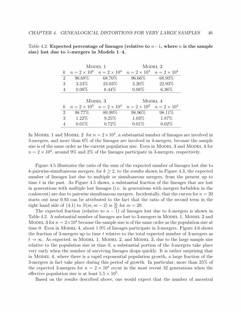
CHAPTER 4. GENEALOGICAL DISTORTIONS FOR VERY LARGE SAMPLES 46
Table 4.2: Expected percentage of lineages (relative to n−1, where n is the samplesize) lost due to k-mergers in Models 1–4.
Model 1 Model 2k n = 2× 10³ n = 2× 10⁴ n = 2× 10³ n = 2× 10⁴
2 96.68% 68.70% 96.66% 68.93%3 3.24% 23.03% 3.26% 22.93%4 0.08% 6.44% 0.08% 6.36%
Model 3 Model 4k n = 2× 10³ n = 2× 10⁴ n = 2× 10³ n = 2× 10⁴
2 98.77% 89.99% 98.96% 98.11%3 1.22% 9.25% 1.03% 1.87%4 0.01% 0.72% 0.01% 0.02%
In Model 1 and Model 2 for n = 2×10⁴, a substantial number of lineages are involved in3-mergers, and more than 6% of the lineages are involved in 4-mergers, because the samplesize is of the same order as the current population size. Even in Model 3 and Model 4 forn = 2× 10⁴, around 9% and 2% of the lineages participate in 3-mergers, respectively.
Figure 4.5 illustrates the ratio of the sum of the expected number of lineages lost due tok-pairwise-simultaneous mergers, for k ≥ 2, to the results shown in Figure 4.3, the expectednumber of lineages lost due to multiple or simultaneous mergers, from the present up totime t in the past. As Figure 4.5 shows, a substantial fraction of the lineages that are lostin generations with multiple lost lineages (i.e. in generations with mergers forbidden in thecoalescent) are due to pairwise simultaneous mergers. Incidentally, that the curves for n = 20starts out near 0.93 can be attributed to the fact that the ratio of the second term in theright hand side of (4.1) to S(m,m− 2) is 51
55for m = 20.
The expected fraction (relative to n − 1) of lineages lost due to k-mergers is shown inTable 4.2. A substantial number of lineages are lost to 3-mergers in Model 1, Model 2 andModel 3 for n = 2×10⁴ because the sample size is of the same order as the population size attime 0. Even in Model 4, about 1.9% of lineages participate in 3-mergers. Figure 4.6 showsthe fraction of 3-mergers up to time t relative to the total expected number of 3-mergers ast→∞. As expected, in Model 1, Model 2, and Model 3, due to the large sample sizerelative to the population size at time 0, a substantial portion of the 3-mergers take placevery early when the number of surviving lineages drops quickly. It is rather surprising thatin Model 4, where there is a rapid exponential population growth, a large fraction of the3-mergers in fact take place during this period of growth. In particular, more than 25% ofthe expected 3-mergers for n = 2 × 10⁴ occur in the most recent 32 generations when theeffective population size is at least 5.5× 10⁵.
Based on the results described above, one would expect that the number of ancestral

CHAPTER 4. GENEALOGICAL DISTORTIONS FOR VERY LARGE SAMPLES 47
lineages remaining at a given time decreases more rapidly under the DTWF model thanunder the coalescent, and we investigate this quantity next.
4.3 Number of lineages as a function of time
Here, we compare the expected number of lineages as a function of time (NLFT) in thecoalescent and in the DTWF model. In what follows, we let ACn (t) and ADn (t) denote therandom variables for the number of lineages at generation t in the coalescent and the DTWFmodel, respectively, starting with a sample of size n at time 0. Under the coalescent, theexpectation and standard deviation of the NLFT, E[ACn (t)] and σ(ACn (t)), can be computedexactly in a numerically-stable fashion for an arbitrary variable population size model asdescribed in Section 4.6.5. An algorithm to compute E[ADn (t)] and σ(ADn (t)) under theDTWF model is also described there.
For the four demographic models considered, Figure 4.7 shows the expectation and stan-dard deviation of the NLFT under the DTWF model, while Figures 4.8 and 4.9 show therelative differences in the expectation and standard deviation, respectively, of the NLFT inthe coalescent with respect to the NLFT in the DTWF model. For large sample sizes underModel 1, Model 2, and Model 3, it can be seen that the lineages are lost at a faster ratein the DTWF model than in the coalescent. This pattern is consistent with the fact thatthese demographic models exhibit a substantial number of 3-mergers in the DTWF modelfor large sample sizes (see Table 4.2), though the deviation in the expected NLFT is stillsubstantially less than the expected number of 3-mergers. The deviation disappears afterabout 1000 generations when enough time has passed for the number of ancestral lineagesto become sufficiently small that the coalescent approximation holds.
For Model 4, the expected NLFT in the coalescent provides a fairly good approximationto that in the DTWF model for all times and for all sample sizes considered. This is becausethe population size remains much larger than the number of ancestral lineages at all times.
4.4 Expected sample frequency spectrum
Given a sample of n haploid (or n/2 diploid) individuals, a common summary of the sam-ple used in various population genetic analyses is the sample frequency spectrum, τ n =(τn,1, . . . , τn,n−1). Under the infinite-sites model of mutation, the kth entry τn,k correspondsto the number of polymorphic sites in the sample that have k derived alleles and n − kancestral alleles, where 1 ≤ k ≤ n − 1. For a sample of n haploids randomly drawn fromthe population, we denote the expected value of τn,k in the coalescent and the DTWF mod-els by τCn,k and τDn,k, respectively. In the case of a constant population size, τCn,k under theinfinite-sites model of mutation is given exactly by the expression
τCn,k =θ
k, (4.2)

CHAPTER 4. GENEALOGICAL DISTORTIONS FOR VERY LARGE SAMPLES 48
where θ denotes a population-scaled mutation rate. (Mutations arise according to a Poissonprocess with intensity θ/2 in each lineage, independently of all other lineages.) For variablepopulation size models, the results of Polanski and Kimmel [69] can be used to computethe expected sample frequency spectrum numerically-stably under the coalescent. In Sec-tion 4.6.4, we develop an algorithm to compute the expected sample frequency spectrumunder the DTWF model, denoted by τDn = (τDn,1, . . . , τ
Dn,n−1).
Figure 4.10 illustrates the relative difference between the coalescent and the DTWF modelin the number of singletons (τn,1) and doubletons (τn,2) as a function of the sample size (n). Asthe figure shows, the number of singletons predicted by the DTWF model is larger than thecoalescent prediction by as much as 11% when the sample size is comparable to the currentpopulation size. It is interesting to note that even though there are a substantial numberof 3-mergers and 4-mergers in Model 1 and Model 2, the deviations in the frequencyspectrum are not nearly as large as one might have expected. This is probably becauseeven though the coalescent forbids multiple mergers by construction, successive two mergerscan be separated by arbitrarily small amounts of time (as opposed to being separated by atleast 1 generation in a discrete model). This allows the coalescent to simulate the effect ofmultiple mergers without explicitly allowing them, leading to fairly similar frequency spectraas a DTWF model.
The deviations in the singletons and doubletons for Model 1match those computed by Fisher [18] (and tabulated in [90, Table 1]) when the samplesize equals the population size and in the limit that the population size tends to infinity.For Model 4 (Figure 4.10d), we could not consider sample sizes > 105 because of compu-tational burden, but the results for Models 1–3 suggest that we should expect to observe≥ 10% deviation when the sample size n is increased to 106, the current population size inModel 4. The deviation in the number of doubletons is also significant when the samplesize is comparable to the current population size; the DTWF prediction for doubletons issmaller than the coalescent prediction by about 4.8%.
The findings described above are especially important given that rare variants comprisea large fraction of segregating sites when the sample size is large. In Figure 4.11, we plot thecumulative distribution of the frequency spectrum in the DTWF model for Models 1–4.The number of singletons in Models 3 and 4 is higher than in Models 1 and 2 due to ex-ponential population growth. The rapid population expansion in Model 4 results in about51% of the segregating sites being singletons and over 80% of the segregating sites havingless than 5 copies of the derived allele in a sample of size n = 2 × 10⁴. Figure 4.12 showsthe expected proportion of rare variants (derived allele frequency ≤ 0.01%) as a functionof the sample size n for Models 3 and 4 under the coalescent. It can be seen that as napproaches the current population size, the proportion of rare variants increases substan-tially. Figure 4.13 shows the expected proportion of segregating sites that are singletons as afunction of n for Models 1–4 under the coalescent. For small sample sizes (say, n < 100),the proportion of singletons in Model 3 and 4 (which incorporate rapid recent populationexpansion) is not much larger than that in Models 1 and 2. However, the difference in-creases considerably as the sample size goes beyond a few hundred individuals, illustrating

CHAPTER 4. GENEALOGICAL DISTORTIONS FOR VERY LARGE SAMPLES 49
the need for large sample sizes to infer recent population expansion from frequency spectrumdata.
4.5 A hybrid method for computing the frequency
spectrum
As detailed in Section 4.6, computation in the DTWF model is substantially more involvedthan in the coalescent. In particular, while the runtime of the frequency spectrum compu-tation in the coalescent depends only on the number of piecewise-exponential epochs andnot the duration of each epoch, the runtime of our dynamic programming algorithm for theDTWF model actually depends on the number of generations over which the algorithm isrun. Since noticeable deviation between the DTWF model and the coalescent arises whenthe number of ancestral lineages is not negligible compared to the population size, a reason-able tradeoff between accuracy and runtime would be to use the DTWF model for the recentpast and the coalescent for the more distant past (when the number of ancestral lineages hasdecreased sufficiently).
To explore this idea, we implemented a hybrid method for computing the frequencyspectrum which, for a specified switching generation ts, uses the full DTWF model forgenerations 0 < t ≤ ts, followed by the coalescent for generations t > ts. In particular,for ts = 0, this algorithm computes the frequency spectrum under the coalescent, while forts =∞, it computes the frequency spectrum under the full DTWF model.
As Figure 4.14 illustrates for Model 3 in the case the sample size n is equal to thecurrent effective population size N0, the difference in the frequency spectrum between thefull DTWF model and the hybrid algorithm decreases rapidly as ts increases. With ts = 5generations, the largest deviation in the number of singletons is less than 1%, which is asubstantial reduction from 11% for ts = 0 (Figure 4.10c). Figure 4.15 shows these data in adifferent way, where the deviations in the frequency spectrum for Model 3 between the fullDTWF model and the hybrid algorithm are shown as a function of sample size for severalvalues of ts.
4.6 Computational details
In this section, we present the details of the algorithms used to compute the various quantitiessuch as the expected NLFT, the expected number of k-mergers and the sample frequencyspectrum under the DTWF model, and the NLFT under the coalescent.
4.6.1 Notation
Let N(t) be the number of (haploid) individuals at generation t in a DTWF model, where
t = 0 corresponds to the present and t is increasing going back in the past. Let p(t)n,m denote

CHAPTER 4. GENEALOGICAL DISTORTIONS FOR VERY LARGE SAMPLES 50
the probability that a sample of n labeled individuals at generation t has m distinct ancestorsat generation t + 1. The probabilities p
(t)n,m can be computed using the following recursion
for 1 ≤ m ≤ n,
p(t)n,m =
N(t+ 1)−m+ 1
N(t+ 1)p
(t)n−1,m−1 +
m
N(t+ 1)p
(t)n−1,m, (4.3)
with the convention that p(t)0,0 := 1, and p
(t)n,m = 0 for all other values of m and n. This
recursion can be derived by treating a sample of size n as a sample of size n − 1 and anadditional individual. The first term of (4.3) is the probability that the parent of thisindividual is distinct from the m − 1 parents of the n − 1 individuals in the sample, andthe second term of (4.3) is the probability that the parent of this individual is one of the mparents of the n− 1 individuals in the sample.
For an algorithmic reason that will become clear presently, we assume that there is acritical generation tc such that N(t) = N (some constant) for all t > tc. This assumptionis not so restrictive since for sufficiently large t, there will be only 1 lineage left with highprobability, and the genealogical properties we study will not be affected. For t > tc, wedrop the dependence on t in the probabilities p
(t)n,m, and simply write them as pn,m.
4.6.2 Expected number of lineages as a function of time underthe DTWF model
By conditioning on the number of ancestral lineages in the previous generation, it is easyto write a recurrence relation for the distribution of the number of lineages at generation tgiven that there are n lineages at time 0,
P[ADn (t) = m] =
∑nk=m p
(t−1)k,m P[ADn (t− 1) = k], if t > 0,
δn,m, if t = 0,(4.4)
where δn,m = 1 if n = m, and δn,m = 0 otherwise. One can then compute the expectationE[ADn (t)] using (4.4).
4.6.3 Expected number of multiple- and simultaneous-mergers inthe DTWF model
Let M(t)n,k be the random variable denoting the number of k-mergers that occur in a genealog-
ical tree starting with a sample of size n observed at generation t. The expected number ofk-mergers in a sample of size n observed at present, E[M
(0)n,k], can be computed by condition-
ing on the mergers that occur between generation t and t + 1. We then have the followingrecurrence relations for E[M
(t)n,k],
E[M(t)n,k] =
(nk
)∑nm=k+1 p
(t)k,1p
(t)n−k,m−k
N(t+1)−m+kN(t+1)
+∑n
m=1 p(t)n,mE[M
(t+1)m,k ], if k < n,
p(t)k,1 + p
(t)k,kE[M
(t+1)k,k ], if k = n.
(4.5)

CHAPTER 4. GENEALOGICAL DISTORTIONS FOR VERY LARGE SAMPLES 51
If the population size is constant, or for t > tc when the population size remains fixed inthe past, we can drop the dependence on t in the notation E[M
(t)n,k], and derive the following
recurrence relations and boundary conditions for E[Mn,k]:
E[Mn,k] =
(nk
)∑nm=k+1
pk,1pn−k,m−k
1−pn,n
N−m+kN
+∑n−1
m=1pn,m
1−pn,nE[Mm,k], if k < n,
pk,11−pk,k , if k = n.
(4.6)
One can write similar recurrence relations for the expected number of k-simultaneous mergersby conditioning on the mergers that occur during each generation of reproduction.
4.6.4 Expected sample frequency spectrum under the DTWFmodel
The expected frequency spectrum of a randomly drawn sample of n individuals is denotedτ n = (τn,1, . . . , τn,n−1), where τn,k corresponds to the number of polymorphic sites in thesample having k derived alleles and n − k ancestral alleles for 1 ≤ k < n under an infinite-sites model of mutation. For a given sample of individuals observed at present, the ancestralprocess in the DTWF model generates a genealogical tree, where the root of the tree is themost recent common ancestor (MRCA) of the sample, with the individuals in the sampleforming the leaves of the tree. For the DTWF model, we can use dynamic programming toefficiently calculate τn,k as follows. Let γ
(t)a,b be a random variable denoting the total branch
length (in number of generations) of a subtree that subtends a particular set of a labeledindividuals in a larger set of a+b individuals observed at time t. Then by the exchangeabilityof the individuals in the sample, the definition of γ, and linearity of expectation, we have,
τn,k =θ
2
(n
k
)E[γ
(0)k,n−k], (4.7)
since there are(nk
)subsamples of k individuals out of the n individuals in the original sample.
By conditioning on the mergers between lineages that take place between generations t andt+ 1, we get the following recurrence relations for E[γ
(t)a,b],
E[γ(t)a,b] =
∑a
j=1
∑bk=1 p
(t)a,jp
(t)b,k
(N(t+1)−j)k↓(N(t+1))k↓
E[γ(t+1)j,k ] if a > 1,
1 +∑b
m=1N(t+1)−mN(t+1)
p(t)b,mE[γ
(t+1)1,m ] if a = 1 and b > 1,
1 + p(t)2,2E[γ
(t+1)1,1 ] if a = b = 1.
(4.8)
If the population size is constant, or for t > tc when the population size remains fixed inthe past, we can drop the dependence on t in the notation γ
(t)a,b, and by conditioning on the
previous genealogical event, we can derive the following recurrence relations and boundaryconditions for E[γa,b],
E[γa,b] =
∑a
j=1
∑bk=1(1− δj,aδk,b) pa,jpb,k
1−pa+b,a+b
(N−j)k↓(N)k↓
E[γj,k] if a > 1,1
1−pb+1,b+1+∑b−1
m=1N−mN
pb,m1−pb+1,b+1
E[γ1,m] if a = 1 and b > 1,
N if a = b = 1.
(4.9)

CHAPTER 4. GENEALOGICAL DISTORTIONS FOR VERY LARGE SAMPLES 52
From recurrence relations (4.8) and (4.9), the expected frequency spectrum for a sampleof size n can be computed in O(n4) and O(n4tc) time for the constant and variable populationcases respectively. However, if one truncates the summation range for the indices j and kin (4.8) and (4.9) to only those j, k values where p
(t)a,j and p
(t)b,k (respectively, pa,j and pb,k)
are greater than some small tolerance parameter ε > 0, the time complexity of the abovedynamic programs can be improved to O(n2) and O(n2tc), where the O notation signifiesthe dependence of the quantities on the truncation parameter ε.
We used (4.7) along with a truncation parameter of ε = 10−120 to compute the expectedfrequency spectra values presented in the Results. Upon decreasing this threshold further, wedid not observe any change to the frequency spectra, suggesting that the computed answersare accurate.
4.6.5 Expected number of lineages as a function of time underthe coalescent
Suppose we have a panmictic population with size N(t) at time t, evolving according toKingman’s coalescent. If we sample n lineages at time 0 and let ACn (t) denote the number ofancestral lineages of this sample surviving at time t, then we have the following expressionfor the probability distribution function of ACn (t) [83, 84],
P[ACn (t) = m] =n∑
i=m
e−(i2)R(t)(−1)i−m
(2i− 1)(m)(i−1)↑(n)i↓m!(i−m)!(n)i↑
, (4.10)
where
R(t) =
∫ t
0
N(0)
N(τ)dτ. (4.11)
The summation in (4.10) has terms with alternating signs, and this leads to a loss of numer-ical precision due to catastrophic cancellation for even moderate sample sizes [56]. Hence,computing the expectation of the NLFT, E[An(t)], by naively using (4.10) will not producereliable answers. However, using a formula of Tavare [84, equation 5.11], one gets the follow-ing closed-form expressions for the expectation and variance of An(t) that are numericallystable to evaluate,
E[ACn (t)] =n∑i=1
e−(i2)R(t)(2i− 1)
(n)i↓(n)i↑
, (4.12)
Var(ACn (t)
)=
n∑i=1
e−(i2)R(t)(2i− 1)(i2 − i+ 1)
(n)i↓(n)i↑
−[
n∑i=1
e−(i2)R(t)(2i− 1)
(n)i↓(n)i↑
]2
. (4.13)
Each term in the summations in (4.12) and (4.13) is positive, and hence poses no numericalproblems for evaluation. Furthermore, the terms in the sum decay rapidly for large i due tothe exponential functions involved. We give elementary combinatorial proofs of (4.12) and(4.13) in Section A.2 of Appendix A.

CHAPTER 4. GENEALOGICAL DISTORTIONS FOR VERY LARGE SAMPLES 53
4.7 Dicussion
Several analyses of genomic sequence variation in large samples of humans [19,39,62,85] havefound a substantial excess of rare variation compared to those predicted using previously ap-plied demographic models. The inference in these studies is that these results are consistentwith a rapid growth of the effective population size in the recent past (much more rapid thanin previously applied demographic models), a conclusion consistent with historical records ofcensus population size [39]. These studies also employed sample sizes that would appear tobe large enough to violate assumptions of the coalescent, potentially distorting genealogicalproperties in a way that may inflate rare variation relative to the predictions of coalescenttheory. In this chapter, we have investigated this issue by developing a method for perform-ing exact computation in the discrete-time Wright-Fisher model of random mating. We havestudied the deviation between the coalescent and the Wright-Fisher model for several keygenealogical quantities that are used for population genomic inference.
For several recently inferred demographic scenarios for humans, our results show thatthere are a significant number of multiple- and simultaneous-merger events under the Wright-Fisher model that are ignored by construction of the coalescent. Furthermore, there are no-ticeable differences in the expected number of rare variants between the coalescent and theDTWF model, especially in the regime where the sample size is on the order of the currenteffective population size. Even if the demographic models considered here might underesti-mate the true current effective population size of humans, sample sizes in population geneticstudies are rapidly increasing and might grow to be large enough to cause the differencesbetween the DTWF and the coalescent to become amplified.
A number of demographic inference methods are based on fitting the expected frequencyspectra under the coalescent [12, 62, 85] or the diffusion process [23, 31, 51, 52] to observeddata. For instance, the exponential growth parameters in Models 3 [23] and 4 [85] were in-ferred using a likelihood method based on the diffusion process approximation to the DTWFmodel, by fitting the predicted frequency spectrum to polymorphism patterns observed in asample size of 876 individuals and 2,440 individuals, respectively. Since the diffusion processapproximation to the DTWF model is equivalent to the coalescent approximation, the dif-ferences in the frequency spectrum (see Figure 4.10) between the coalescent and the DTWFmodel indicate that we might infer different demographies if the analysis were done usingthe DTWF model. In particular, for a sample of size n analyzed under the DTWF model,any inferred demography will have a current effective population size of at least n. However,the coalescent imposes no such restriction on the inferred current effective population size.In fact, under the coalescent, it is even possible to estimate a current effective populationsize N0 that is smaller than the sample size n. This is because one can only infer a scalingfunction of time in the coalescent, which is the ratio of the variable effective population sizeto a fixed reference population size. The inferred scaling function can then be transformedinto an effective population size function by using the empirically estimated per-generationmutation rate [23], or by setting the reference population size to a specific value [12,62] (e.g.,using an ancestral population size inferred by previous studies [77]).

CHAPTER 4. GENEALOGICAL DISTORTIONS FOR VERY LARGE SAMPLES 54
To balance the tradeoff between accuracy and computational efficiency, we have proposeda hybrid algorithm that uses the DTWF model for the recent past and the coalescent for themore distant past. This hybrid algorithm provides a way to obtain more accurate predic-tions of the frequency spectrum than in the coalescent, while being computationally moreefficient than considering the full DTWF model. We leave the exploration of this methodfor demographic inference as future research.
Wakeley and Takahashi [90] have provided asymptotically accurate expressions (as theeffective population size N →∞) for the number of singletons and the number of segregatingsites under a variant of the DTWF model which allows for a larger number of offspringthan the effective population size, assuming that the effective population size stays constantover time. Fu [21] has also examined the accuracy of the standard coalescent model andproposed an alternative continuous-time “exact” coalescent model applicable in the regimewhen N(N−1) · · · (N−n+1)×N−n 0, where N denotes the effective population size andn the sample size. That work was restricted to the case of a constant population size, while inthis chapter we have considered several demographic scenarios inferred from recent large-scalepopulation genomic studies. Moreover, for some of the demographic scenarios and samplesizes considered here, the assumption in Fu’s work [21] thatN(N−1) · · · (N−n+1)×N−n 0is violated. Wakeley et al. [89] have shown that it is difficult to reject the coalescent evenfor data generated using fixed pedigrees with random genetic assortment. Our work iscomplementary to that study and compares the coalescent to the DTWF random matingmodel.
In this chapter, we have focused on the DTWF model for simplicity. However, it isknown that under some weak conditions on the limiting probabilities of a 2-merger anda 3-merger, a large family of exchangeable random mating models converge to the samecoalescent limit as the unit of time is rescaled appropriately and the population size gets large[58, 59]. The rate of convergence to the coalescent differs between different random matingmodels [4], and hence the accuracy of coalescent predictions for large sample sizes dependson the random mating model being considered. The deviation from the coalescent could beamplified for other random-mating models. It would be interesting to consider the accuracyof the coalescent for other random and realistic models of relevance to human genetics; e.g.,models in which generations overlap and the distribution of offspring number more closelyreflects the observed pattern for human populations (for example, the Swedish family dataof Low and Clarke [50] or the Saguenay-Lac-Saint-Jean population considered by Moreau etal. [60]). Despite having access to large samples, recent studies [19,62,85] have inferred muchsmaller current effective population sizes (on the order of millions) than the current censussize (on the order of billions) of the population from which the samples were drawn. It ispossible that demographic inference methods that explicitly model realistic human matingpatterns might be able to infer census population size histories more accurately than doesthe coalescent, which assumes random mating and can only infer effective population sizesthat do not have a direct census interpretation.
Furthermore, it would be interesting to compare discrete-time random models and thecoalescent with respect to haplotype sharing (identity-by-descent and identity-by-state), link-

CHAPTER 4. GENEALOGICAL DISTORTIONS FOR VERY LARGE SAMPLES 55
age disequilibrium, and natural selection when the sample size is very large. For example,Davies et al. [13] employed simulations to demonstrate that for a constant population sizemodel, recombination and gene conversion can increase the number of ancestral lineages of asample of chromosomes to the extent that multiple and simultaneous mergers in the DTWFmodel can lead to substantial differences from the coalescent model in the rates of coales-cence and in the number of sequences carrying ancestral material. It would be interesting toperform such comparisons for more realistic demographic models for humans.
We will soon enter an era where it will become routine to analyze samples with hun-dreds of thousands if not millions of individuals. For these large sample sizes, the standardcoalescent will no longer serve as an adequate model for evolution. The DTWF modelis mathematically cumbersome to work with, which was one of the original motivationsfor adopting the coalescent for modern population genetics analyses. However, for thesevery large sample sizes, we will need to develop new mathematically and computationallytractable stochastic processes that better approximate realistic models of human populationevolution, and under which we can efficiently compute genealogical quantities like we havebeen able to under the coalescent.

CHAPTER 4. GENEALOGICAL DISTORTIONS FOR VERY LARGE SAMPLES 56
0 1000 2000 3000 4000 5000Time t (in generations)
0.0
0.2
0.4
0.6
0.8
1.0
Exp
ecte
dfr
acti
on
n = 20
n = 2× 10²
n = 2× 10³
n = 2× 10⁴
(a)
0 1000 2000 3000 4000 5000Time t (in generations)
0.0
0.2
0.4
0.6
0.8
1.0
Exp
ecte
dfr
acti
on
n = 20
n = 2× 10²
n = 2× 10³
n = 2× 10⁴
(b)
0 1000 2000 3000 4000 5000 6000Time t (in generations)
0.0
0.2
0.4
0.6
0.8
1.0
Exp
ecte
dfr
acti
on
n = 20
n = 2× 10²
n = 2× 10³
n = 2× 10⁴
(c)
0 1000 2000 3000 4000 5000 6000Time t (in generations)
0.0
0.2
0.4
0.6
0.8
1.0E
xpec
ted
frac
tion
n = 20
n = 2× 10²
n = 2× 10³
n = 2× 10⁴
(d)
Figure 4.3: Expected proportion of lineages (relative to n−1, where n is the samplesize at present) that are lost in generations when more than one lineage is lost,from the present up to time t in the past. For each generation t on the x-axis, they-axis is the expected number of lineages that have been lost due to coalescence events inthose generations from 0 to t where more than one lineage is lost, normalized by the quantityn − 1, which is the total number of lineages that are lost over all generations. The plotscorrespond to (a) Model 1, (b) Model 2, (c) Model 3, and (d) Model 4. The sharpjumps in the plot for Model 2((b)) corresponds to the beginning (backwards in time) ofpopulation bottlenecks when the population size declines substantially, thus instantaneouslyincreasing the rate at which lineages find common ancestors and are lost. For small samplesizes relative to the population size (n = 20 and n = 200), it is unlikely for more than onelineage to be lost in a single generation. In contrast, for large sample sizes (n = 2 × 10⁴),almost all the lineages are lost in generations when more than one lineage is lost.

CHAPTER 4. GENEALOGICAL DISTORTIONS FOR VERY LARGE SAMPLES 57
· · · · · ·
2(m− j) 2j −m
m
j
generation t
generation t+ 1
Figure 4.4: An example generation of an (m − j)-pairwise-simultaneous mergerduring which m lineages in generation t find j parents in generation t+ 1 (back-wards in time). Each of m − j pairs of lineages in generation t finds a different commonparent in generation t + 1, while the remaining 2j −m lineages of generation t each have adifferent parent in generation t+ 1.

CHAPTER 4. GENEALOGICAL DISTORTIONS FOR VERY LARGE SAMPLES 58
0 1000 2000 3000 4000 5000Time t (in generations)
0.0
0.2
0.4
0.6
0.8
1.0
Fra
ctio
n n = 20
n = 2× 10²
n = 2× 10³
n = 2× 10⁴
(a)
0 1000 2000 3000 4000 5000Time t (in generations)
0.0
0.2
0.4
0.6
0.8
1.0
Fra
ctio
n n = 20
n = 2× 10²
n = 2× 10³
n = 2× 10⁴
(b)
0 1000 2000 3000 4000 5000 6000Time t (in generations)
0.0
0.2
0.4
0.6
0.8
1.0
Fra
ctio
n n = 20
n = 2× 10²
n = 2× 10³
n = 2× 10⁴
(c)
0 1000 2000 3000 4000 5000 6000Time t (in generations)
0.2
0.3
0.4
0.5
0.6
0.7
0.8
0.9
1.0
Fra
ctio
n n = 20
n = 2× 10²
n = 2× 10³
n = 2× 10⁴
(d)
Figure 4.5: Ratio of the sum of the expected number of lineages lost due to k-pairwise-simultaneous mergers up to time t, for k ≥ 2, to the respective resultsshown in Figure 4.3. This quantity measures the proportion of lineages lost in generationswhere more than one lineage is lost due to pairwise simultaneous merger events (and nomultiple merger events). The plots correspond to (a) Model 1, (b) Model 2, (c) Model 3,and (d) Model 4. A substantial fraction of the lineages that are lost in generations withmultiple lost lineages are due to pairwise simultaneous mergers.

CHAPTER 4. GENEALOGICAL DISTORTIONS FOR VERY LARGE SAMPLES 59
0 100 200 300 400 500 600 700 800Time t (in generations)
0.0
0.2
0.4
0.6
0.8
1.0
Fra
ctio
n
n = 2× 10³
n = 2× 10⁴
(a)
0 100 200 300 400 500 600 700 800Time t (in generations)
0.0
0.2
0.4
0.6
0.8
1.0
Fra
ctio
n
n = 2× 10³
n = 2× 10⁴
(b)
0 100 200 300 400 500 600 700 800Time t (in generations)
0.0
0.2
0.4
0.6
0.8
1.0
Fra
ctio
n
n = 2× 10³
n = 2× 10⁴
(c)
0 100 200 300 400 500 600 700 800Time t (in generations)
0.0
0.2
0.4
0.6
0.8
1.0
Fra
ctio
n
n = 2× 10³
n = 2× 10⁴
(d)
Figure 4.6: Ratio of the expected number of 3-mergers until time t to the totalexpected number of 3-mergers. The plots correspond to (a) Model 1, (b) Model 2,(c) Model 3, and (d) Model 4. In Model 1 and Model 2, due to the large sample sizerelative to the population size at time 0, a substantial portion of the 3-mergers take placevery early when the number of surviving lineages drops quickly. Even in Model 4 wherethere is a rapid exponential population growth in the most recent 204 generations, morethan 25% of the expected 3-mergers for n = 2× 10⁴ occur in the most recent 32 generationswhen the effective population size is at least 5.5× 10⁵ haploids.

CHAPTER 4. GENEALOGICAL DISTORTIONS FOR VERY LARGE SAMPLES 60
0 1000 2000 3000 4000 5000Time t (in generations)
0.0
0.2
0.4
0.6
0.8
1.0
1.2
E[ADn (t)]n
n = 20
n = 2× 10²
n = 2× 10³
n = 2× 10⁴
(a)
0 1000 2000 3000 4000 5000Time t (in generations)
0.0
0.2
0.4
0.6
0.8
1.0
1.2
E[ADn (t)]n
n = 20
n = 2× 10²
n = 2× 10³
n = 2× 10⁴
(b)
0 1000 2000 3000 4000 5000 6000Time t (in generations)
0.0
0.2
0.4
0.6
0.8
1.0
1.2
E[ADn (t)]n
n = 20
n = 2× 10²
n = 2× 10³
n = 2× 10⁴
(c)
0 1000 2000 3000 4000 5000 6000Time t (in generations)
0.0
0.2
0.4
0.6
0.8
1.0
1.2
E[ADn (t)]n
n = 20
n = 2× 10²
n = 2× 10³
n = 2× 10⁴
(d)
Figure 4.7: The expectation (solid line) and standard deviation (vertical whiskers)of the NLFT under the DTWF model. (a) Model 1. (b) Model 2. (c) Model 3.(d) Model 4.

CHAPTER 4. GENEALOGICAL DISTORTIONS FOR VERY LARGE SAMPLES 61
0 200 400 600 800 1000Time t (in generations)
−7
−6
−5
−4
−3
−2
−1
0
E[A
D n(t
)]−E
[AC n
(t)]
E[A
D n(t
)]×
100%
n = 20
n = 2× 10²
n = 2× 10³
n = 2× 10⁴
(a)
0 200 400 600 800 1000Time t (in generations)
−7
−6
−5
−4
−3
−2
−1
0
E[A
D n(t
)]−E
[AC n
(t)]
E[A
D n(t
)]×
100%
n = 20
n = 2× 10²
n = 2× 10³
n = 2× 10⁴
(b)
0 500 1000 1500 2000 2500Time t (in generations)
−2.5
−2.0
−1.5
−1.0
−0.5
0.0
E[A
D n(t
)]−E
[AC n
(t)]
E[A
D n(t
)]×
100%
n = 20
n = 2× 10²
n = 2× 10³
n = 2× 10⁴
(c)
0 500 1000 1500 2000 2500Time t (in generations)
−1.5
−1.0
−0.5
0.0
E[A
D n(t
)]−E
[AC n
(t)]
E[A
D n(t
)]×
100%
n = 20
n = 2× 10²
n = 2× 10³
n = 2× 10⁴
(d)
Figure 4.8: The percentage difference in the expected NLFT between the coales-cent and DTWF models, for a haploid sample of size n ∈ 20, 2×10², 2×10³, 2×10⁴.The plots correspond to (a) Model 1, (b) Model 2, (c) Model 3, and (d) Model 4. Forall demographic models, lineages are lost at a faster rate in the DTWF model than in thecoalescent, consistent with the fact that there are a substantial number of 3-mergers in theDTWF model for large sample sizes. This deviation is more pronounced for larger samplesizes and for Models 1–3 where the sample size is comparable to the current populationsize.

CHAPTER 4. GENEALOGICAL DISTORTIONS FOR VERY LARGE SAMPLES 62
0 200 400 600 800 1000Time t (in generations)
−30
−25
−20
−15
−10
−5
0
σ[A
D n(t
)]−σ
[AC n
(t)]
σ[A
D n(t
)]×
100%
n = 20
n = 2× 10²
n = 2× 10³
n = 2× 10⁴
(a)
0 200 400 600 800 1000Time t (in generations)
−30
−25
−20
−15
−10
−5
0
σ[A
D n(t
)]−σ
[AC n
(t)]
σ[A
D n(t
)]×
100%
n = 20
n = 2× 10²
n = 2× 10³
n = 2× 10⁴
(b)
0 500 1000 1500 2000 2500Time t (in generations)
−6
−5
−4
−3
−2
−1
0
σ[A
D n(t
)]−σ
[AC n
(t)]
σ[A
D n(t
)]×
100%
n = 20
n = 2× 10²
n = 2× 10³
n = 2× 10⁴
(c)
0 500 1000 1500 2000 2500Time t (in generations)
−2.0
−1.5
−1.0
−0.5
0.0
0.5
σ[A
D n(t
)]−σ
[AC n
(t)]
σ[A
D n(t
)]×
100%
n = 20
n = 2× 10²
n = 2× 10³
n = 2× 10⁴
(d)
Figure 4.9: The percentage difference in the standard deviation of the NLFTbetween the coalescent and DTWF models, for a haploid sample of size n ∈20, 2 × 10², 2 × 10³, 2 × 10⁴. The plots correspond to (a) Model 1, (b) Model 2, (c)Model 3, and (d) Model 4.

CHAPTER 4. GENEALOGICAL DISTORTIONS FOR VERY LARGE SAMPLES 63
101 102 103 104 105
Sample size n
−6
−4
−2
0
2
4
6
8
10
12
τD n,i−τC n,i
τD n,i×
100%
SingletonsDoubletons
(a)
101 102 103 104 105
Sample size n
−6
−4
−2
0
2
4
6
8
10
12
τD n,i−τC n,i
τD n,i×
100%
SingletonsDoubletons
(b)
101 102 103 104 105
Sample size n
−6
−4
−2
0
2
4
6
8
10
12
τD n,i−τC n,i
τD n,i×
100%
SingletonsDoubletons
(c)
101 102 103 104 105
Sample size n
−0.4
−0.2
0.0
0.2
0.4
0.6
0.8
1.0
1.2
1.4
τD n,i−τC n,i
τD n,i×
100%
SingletonsDoubletons
(d)
Figure 4.10: The percentage relative error in the number of singletons and dou-bletons between the coalescent and DTWF models, as a function of the samplesize n. When the sample size is comparable to the current population size, the numberof singletons predicted by the DTWF model is larger than the coalescent prediction by asmuch as 11%, while the number of doubletons predicted by the DTWF model is smallerthan the coalescent prediction by about 4.8%. In Model 4, we could not consider a samplesize comparable to the population size (106) because of computational burden, but we expecta similar extent of deviation as in Models 1–3 as n increases. Note that the y-axis scalefor Model 4 is different from that for Models 1–3. (a) Model 1. (b) Model 2. (c)Model 3. (d) Model 4.

CHAPTER 4. GENEALOGICAL DISTORTIONS FOR VERY LARGE SAMPLES 64
0 5 10 15 20 25k, number of derived alleles
0.0
0.2
0.4
0.6
0.8
1.0
Fra
ctio
n
n = 20
n = 2× 10²
n = 2× 10³
n = 2× 10⁴
(a)
0 5 10 15 20 25k, number of derived alleles
0.0
0.2
0.4
0.6
0.8
1.0
Fra
ctio
n
n = 20
n = 2× 10²
n = 2× 10³
n = 2× 10⁴
(b)
0 5 10 15 20 25k, number of derived alleles
0.0
0.2
0.4
0.6
0.8
1.0
Fra
ctio
n
n = 20
n = 2× 10²
n = 2× 10³
n = 2× 10⁴
(c)
0 5 10 15 20 25k, number of derived alleles
0.0
0.2
0.4
0.6
0.8
1.0
Fra
ctio
n
n = 20
n = 2× 10²
n = 2× 10³
n = 2× 10⁴
(d)
Figure 4.11: The cumulative distribution function of the frequency spectrum, asa function of the number of derived alleles, k, in the DTWF model with samplesizes n ∈ 20, 2 × 10², 2 × 10³, 2 × 10⁴. For each value of k on the x-axis, the y-axis isthe proportion of segregating sites with at most k copies of the derived allele in the DTWF
model,∑k
j=1 τDn,j∑n−1
i=1 τDn,i
. The plots correspond to (a) Model 1, (b) Model 2, (c) Model 3, and
(d) Model 4. In Model 4 where the population grows rapidly in the recent past, about51% of the segregating sites are singletons in a sample of size n = 2× 10⁴. In Model 3, thefraction of singleton sites is lower than in Model 4 because the population growth rate islower.

CHAPTER 4. GENEALOGICAL DISTORTIONS FOR VERY LARGE SAMPLES 65
104 105 106
Sample size n0.2
0.3
0.4
0.5
0.6
0.7
0.8
0.9
1.0
Pro
port
ion
MODEL 3MODEL 4
Figure 4.12: Expected proportion of segregating sites with derived allele frequency≤ 0.01%, as a function of the sample size n in the coalescent for Models 3 and4. The frequency of such rare variants is increasing in the sample size and in the case ofModel 4, rare variants practically account for all the variants for very large sample sizes.

CHAPTER 4. GENEALOGICAL DISTORTIONS FOR VERY LARGE SAMPLES 66
101 102 103 104 105 106
Sample size n0.0
0.1
0.2
0.3
0.4
0.5
0.6
Pro
port
ion
MODEL 1MODEL 2MODEL 3MODEL 4
Figure 4.13: Expected proportion of segregating sites that have only one copy ofthe derived allele (i.e., singletons), as a function of the sample size n in the coa-lescent for Models 1–4. The difference in the number of singletons in Model 4 (whichincorporates recent population expansion) and the number of singletons in Models 1 and2 (without a recent expansion) rapidly increases for sample sizes beyond a few hundred indi-viduals, indicating that large sample sizes are needed to infer demographic models of recentpopulation growth from frequency spectrum data.

CHAPTER 4. GENEALOGICAL DISTORTIONS FOR VERY LARGE SAMPLES 67
0 5 10 15 20Switching time ts
−6
−4
−2
0
2
4
6
8
10
12
τD n,i−τ
(ts)
n,i
τD n,i×
100%
SingletonsDoubletons
Figure 4.14: The percentage relative error, with respect to the full DTWF model,in the number of singletons and doubletons in a hybrid algorithm with switchingtime ts. The hybrid method uses the DTWF model for generations ≤ ts and the coalescentmodel in generations > ts. The results are for Model 3 in the case the sample size n isequal to the current effective population size N0 = 67,627. The case of ts = 0 correspondsto using the coalescent model only. This plot shows that the difference in the frequencyspectrum between the full DTWF model and the hybrid algorithm decreases very rapidly asthe switching time ts increases.

CHAPTER 4. GENEALOGICAL DISTORTIONS FOR VERY LARGE SAMPLES 68
101 102 103 104 105
Sample size n
−0.5
0.0
0.5
1.0
1.5
2.0
2.5
3.0
3.5
4.0
τD n,i−τ
(1)
n,i
τD n,i×
100%
SingletonsDoubletons
(a)
101 102 103 104 105
Sample size n
−0.2
0.0
0.2
0.4
0.6
0.8
1.0
1.2
1.4
τD n,i−τ
(5)
n,i
τD n,i×
100%
SingletonsDoubletons
(b)
101 102 103 104 105
Sample size n
−0.1
0.0
0.1
0.2
0.3
0.4
0.5
0.6
0.7
τD n,i−τ
(10)
n,i
τD n,i×
100%
SingletonsDoubletons
(c)
101 102 103 104 105
Sample size n
−0.10
−0.05
0.00
0.05
0.10
0.15
0.20
0.25
0.30
τD n,i−τ
(25)
n,i
τD n,i×
100%
SingletonsDoubletons
(d)
Figure 4.15: The percentage relative error in the number of singletons and dou-bletons between the computations under the full DTWF model and a hybridalgorithm which uses the coalescent model in generations t > ts for Model 3.The case of ts = 0 corresponds to using the coalescent model only, illustrated in Figure 4.10c.We use τ (ts) to denote the frequency spectrum using the hybrid algorithm with a switchingtime of ts. As ts increases, we see that the deviation between the computation under theDTWF model and the hybrid algorithm decreases monotonically, suggesting that one coulduse such an algorithm to efficiently approximate the frequency spectrum under the DTWFmodel. The values of ts for the plots are (a) ts = 1, (b) ts = 5, (c) ts = 10, (d) ts = 25.

69
Chapter 5
Future directions
This dissertation examined several aspects of demographic inference for a randomly matingpopulation using the sample frequency spectrum of a set of sequences. Beyond the openproblems mentioned in the discussions in each chapter, there are several interesting questionsfor future research related to these aspects:
• What can we say about model identifiability from other representations of genomicdata, such as full haplotype data or the distribution of IBD and IBS tract lengths?Several recent population size inference methods [48, 79] based on the sequentiallyMarkov coalescent approximation [57] implicitly assume that piecewise-constant pop-ulation sizes are identifiable from just two haplotypes. If this is indeed the case, whatis the minimum sequence length required for identifiability under the full coalescentwith recombination or approximations like the sequentially Markov coalescent? Thesame questions can also be asked about the evolutionary models that are used by de-mographic inference methods [34,64] that utilize the distribution of IBS and IBD tractlengths for a pair of haplotypes.
• What can we say about the number of samples sufficient for demographic identifiabilityif we have access to only a few entries of the expected SFS? More generally, how manysamples are sufficient for identifiability given access to a linear transformation of theexpected SFS? Such a result would generalize the identifiability theorem for the foldedfrequency spectrum given in Section 2.3.4 of Chapter 2.
• As the number of segregating sites increases, the empirical SFS converges in probabilityto the expected SFS, thus allowing the demographic model to be reliably inferred fromsample sizes such as those given in Chapter 2. However, if we have access to far moresamples than the minimum needed for identifiability, then simulations indicate thatwe might require fewer segregating sites for reliable inference than if we used a smallersample size. This suggests the following interesting question: for a given total numberof bases of sequencing capacity, what is the trade-off between the sample size andsequence length that maximizes the accuracy of our inference method?

CHAPTER 5. FUTURE DIRECTIONS 70
• Can we develop demographic inference methods based on exact computation that usethe joint SFS from samples from multiple populations while taking into account com-plex demographic events like admixture and continuous migration? Chen [9] has de-rived analytic expressions for the entries of the expected joint SFS of multiple popu-lations that are related by split and point admixture events. It would be interestingto extend those results to the case of multiple populations with continuous migrationbetween them.
• What are the extremal demographic models for the deviations of the various genealog-ical quantities between the discrete-time Wright-Fisher and coalescent models? Whatcan we say about this question for other discrete-time models of mating that also con-verge to the coalescent, such as the discrete-time Moran model or the more generalfamily of Cannings exchangeable models?

71
Bibliography
[1] 1000 Genomes Project Consortium (2010). A map of human genome variationfrom population-scale sequencing. Nature 467, 1061–1073.
[2] Barton, N. H. and Charlesworth, B. (1984). Genetic revolutions, founder effects,and speciation. Annual Review of Ecology and Systematics 15, 133–164.
[3] Bhaskar, A., Clark, A. G. and Song, Y. S. (2013). Distortion of genealogicalproperties when the sample is very large. arXiv:1308.0091 [q-bio].
[4] Bhaskar, A. and Song, Y. S. (2009). Multi-locus match probability in a finitepopulation: a fundamental difference between the Moran and Wright–Fisher models.Bioinformatics 25, i187–i195.
[5] Bhaskar, A. and Song, Y. S. (2013). The identifiability of piecewise demographicmodels from the sample frequency spectrum. arXiv:1309.5056 [q-bio].
[6] Boyko, A. R., Williamson, S. H., Indap, A. R., Degenhardt, J. D., Her-nandez, R. D., Lohmueller, K. E., Adams, M. D., Schmidt, S., Sninsky,J. J., Sunyaev, S. R. et al. (2008). Assessing the evolutionary impact of aminoacid mutations in the human genome. PLoS Genetics 4, e1000083.
[7] Campbell, C. D., Ogburn, E. L., Lunetta, K. L., Lyon, H. N., Freedman,M. L., Groop, L. C., Altshuler, D., Ardlie, K. G. and Hirschhorn, J. N.(2005). Demonstrating stratification in a European American population. Nature Ge-netics 37, 868–872.
[8] Chen, G. K., Marjoram, P. and Wall, J. D. (2009). Fast and flexible simulationof dna sequence data. Genome Research 19, 136–142.
[9] Chen, H. (2012). The joint allele frequency spectrum of multiple populations: Acoalescent theory approach. Theoretical Population Biology 81, 179–195.
[10] Clayton, D. G., Walker, N. M., Smyth, D. J., Pask, R., Cooper, J. D.,Maier, L. M., Smink, L. J., Lam, A. C., Ovington, N. R., Stevens, H. E.et al. (2005). Population structure, differential bias and genomic control in a large-scale, case-control association study. Nature Genetics 37, 1243–1246.

BIBLIOGRAPHY 72
[11] Conrad, D., Keebler, J., DePristo, M., Lindsay, S., Zhang, Y., Casals,F., Idaghdour, Y., Hartl, C., Torroja, C., Garimella, K. et al. (2011).Variation in genome-wide mutation rates within and between human families. Nature201, 1.
[12] Coventry, A., Bull-Otterson, L. M., Liu, X., Clark, A. G., Maxwell,T. J., Crosby, J., Hixson, J. E., Rea, T. J., Muzny, D. M., Lewis, L. R.et al. (2010). Deep resequencing reveals excess rare recent variants consistent withexplosive population growth. Nature Communications 1, 131.
[13] Davies, J. L., Simancık, F., Lyngsø, R., Mailund, T. and Hein, J. (2007).On recombination-induced multiple and simultaneous coalescent events. Genetics 177,2151–2160.
[14] Durrett, R. (2008). Probability models for DNA sequence evolution 2nd ed. Springer,New York.
[15] Erlich, H. A., Bergstrom, T. F., Stoneking, M. and Gyllensten, U. (1996).HLA sequence polymorphism and the origin of humans. Science 274, 1552–1554.
[16] Excoffier, L., Dupanloup, I., Huerta-Sanchez, E., Sousa, V. C. and Foll,M. (2013). Robust demographic inference from genomic and SNP data. PLoS Genetics9, e1003905.
[17] Excoffier, L. and Foll, M. (2011). Fastsimcoal: a continuous-time coalescentsimulator of genomic diversity under arbitrarily complex evolutionary scenarios. Bioin-formatics 27, 1332–1334.
[18] Fisher, R. A. et al. (1930). The distribution of gene ratios for rare mutations.Proceedings of the Royal Society of Edinburgh 50, 205–220.
[19] Fu, W., O’Connor, T. D., Jun, G., Kang, H. M., Abecasis, G., Leal, S. M.,Gabriel, S., Altshuler, D., Shendure, J., Nickerson, D. A. et al. (2012).Analysis of 6,515 exomes reveals the recent origin of most human protein-coding vari-ants. Nature 493, 216–220.
[20] Fu, Y.-X. (1995). Statistical properties of segregating sites. Theoretical PopulationBiology 48, 172–197.
[21] Fu, Y.-X. (2006). Exact coalescent for the Wright-Fisher model. Theoretical PopulationBiology 69, 385–394.
[22] Gantmacher, F. R. (2000). The theory of matrices vol. 2. Chelsea Publishing Com-pany, New York.

BIBLIOGRAPHY 73
[23] Gravel, S., Henn, B. M., Gutenkunst, R. N., Indap, A. R., Marth, G. T.,Clark, A. G., Yu, F., Gibbs, R. A., Bustamante, C. D., Altshuler, D. L.et al. (2011). Demographic history and rare allele sharing among human populations.Proceedings of the National Academy of Sciences 108, 11983–11988.
[24] Griewank, A. and Corliss, G. F. (1991). Automatic differentiation of algorithms:theory, implementation, and application. Society for industrial and Applied Mathemat-ics Philadelphia, PA.
[25] Griffiths, R. (1991). The two-locus ancestral graph. Selected Proceedings of theSheffield Symposium on Applied Probability. IMS Lecture Notes–Monograph Series 18,100–117.
[26] Griffiths, R. (2003). The frequency spectrum of a mutation, and its age, in a generaldiffusion model. Theoretical Population Biology 64, 241–251.
[27] Griffiths, R. and Tavare, S. (1994). Sampling theory for neutral alleles in avarying environment. Philosophical Transactions of the Royal Society of London. SeriesB: Biological Sciences 344, 403–410.
[28] Griffiths, R. and Tavare, S. (1998). The age of a mutation in a general coalescenttree. Communications in Statistics. Stochastic Models 14, 273–295.
[29] Griffiths, R. C. and Marjoram, P. (1997). An ancestral recombination graph.Institute for Mathematics and its Applications 87, 257.
[30] Gusev, A., Lowe, J. K., Stoffel, M., Daly, M. J., Altshuler, D., Breslow,J. L., Friedman, J. M. and Pe’er, I. (2009). Whole population, genome-widemapping of hidden relatedness. Genome Research 19, 318–326.
[31] Gutenkunst, R. N., Hernandez, R. D., Williamson, S. H. and Bustamante,C. D. (2009). Inferring the joint demographic history of multiple populations frommultidimensional SNP frequency data. PLoS Genetics 5, e1000695.
[32] Harding, R. M., Fullerton, S., Griffiths, R. et al. (1997). Archaic Africanand Asian lineages in the genetic ancestry of modern humans. American Journal ofHuman Genetics 60, 772.
[33] Harpending, H. C., Batzer, M. A., Gurven, M. et al. (1998). Genetic traces ofancient demography. Proceedings of the National Academy of Sciences 95, 1961–1967.
[34] Harris, K. and Nielsen, R. (2013). Inferring demographic history from a spectrumof shared haplotype lengths. PLoS Genetics 9, e1003521.
[35] Herbots, H. (1997). The structured coalescent. Progress in Population Genetics andHuman Evolution 87, 231–255.

BIBLIOGRAPHY 74
[36] Hudson, R. (2002). Generating samples under a wright–fisher neutral model of geneticvariation. Bioinformatics 18, 337–338.
[37] Hudson, R. R. (1983). Properties of a neutral allele model with intragenic recombi-nation. Theoretical Population Biology 23, 183–201.
[38] Jameson, G. (2006). Counting zeros of generalised polynomials: Descartes’ rule ofsigns and Laguerre’s extensions. The Mathematical Gazette 90, 223–234.
[39] Keinan, A. and Clark, A. G. (2012). Recent explosive human population growthhas resulted in an excess of rare genetic variants. Science 336, 740–743.
[40] Keinan, A., Mullikin, J. C., Patterson, N. and Reich, D. (2007). Measurementof the human allele frequency spectrum demonstrates greater genetic drift in East Asiansthan in Europeans. Nature Genetics 39, 1251–1255.
[41] Kidd, J. M., Gravel, S., Byrnes, J., Moreno-Estrada, A., Musharoff,S., Bryc, K., Degenhardt, J. D., Brisbin, A., Sheth, V., Chen, R. et al.(2012). Population genetic inference from personal genome data: impact of ancestryand admixture on human genomic variation. The American Journal of Human Genetics91, 660–671.
[42] Kimura, M. (1955). Solution of a process of random genetic drift with a continuousmodel. Proceedings of the National Academy of Sciences 41, 144–150.
[43] Kimura, M. (1969). The number of heterozygous nucleotide sites maintained in a finitepopulation due to steady flux of mutations. Genetics 61, 893.
[44] Kingman, J. F. C. (1982). The coalescent. Stochastic Processes and Their Applications13, 235–248.
[45] Kingman, J. F. C. (1982). Exchangeability and the evolution of large populations.In Exchangeability in probability and statistics. ed. G. Koch and F. Spizzichino. North-Holland Publishing Company pp. 97–112.
[46] Kingman, J. F. C. (1982). On the genealogy of large populations. Journal of AppliedProbability 19, 27–43.
[47] Krone, S. M. and Neuhauser, C. (1997). Ancestral processes with selection. The-oretical Population Biology 51, 210–237.
[48] Li, H. and Durbin, R. (2011). Inference of human population history from individualwhole-genome sequences. Nature 475, 493–496.

BIBLIOGRAPHY 75
[49] Lohmueller, K. E., Indap, A. R., Schmidt, S., Boyko, A. R., Hernandez,R. D., Hubisz, M. J., Sninsky, J. J., White, T. J., Sunyaev, S. R., Nielsen,R. et al. (2008). Proportionally more deleterious genetic variation in European thanin African populations. Nature 451, 994–997.
[50] Low, B. and Clarke, A. (1991). Family patterns in nineteenth-century sweden:impact of occupational status and landownership. Journal of Family History 16, 117–138.
[51] Lukic, S. and Hey, J. (2012). Demographic inference using spectral methods on SNPdata, with an analysis of the human out-of-Africa expansion. Genetics 192, 619–639.
[52] Lukic, S., Hey, J. and Chen, K. (2011). Non-equilibrium allele frequency spectravia spectral methods. Theoretical Population Biology 79, 203–219.
[53] Marchini, J., Cardon, L. R., Phillips, M. S. and Donnelly, P. (2004). Theeffects of human population structure on large genetic association studies. Nature Ge-netics 36, 512–517.
[54] Marjoram, P. and Wall, J. D. (2006). Fast “coalescent” simulation. BMC Genetics7, 16.
[55] Marth, G., Czabarka, E., Murvai, J. and Sherry, S. (2004). The allele fre-quency spectrum in genome-wide human variation data reveals signals of differentialdemographic history in three large world populations. Genetics 166, 351–372.
[56] Maruvka, Y. E., Shnerb, N. M., Bar-Yam, Y. and Wakeley, J. (2011). Re-covering population parameters from a single gene genealogy: An unbiased estimatorof the growth rate. Molecular Biology and Evolution 28, 1617–1631.
[57] McVean, G. A. and Cardin, N. J. (2005). Approximating the coalescent withrecombination. Philosophical Transactions of the Royal Society B: Biological Sciences360, 1387–1393.
[58] Mohle, M. and Sagitov, S. (2001). A classification of coalescent processes forhaploid exchangeable population models. The Annals of Probability 29, 1547–1562.
[59] Mohle, M. and Sagitov, S. (2003). Coalescent patterns in diploid exchangeablepopulation models. Journal of Mathematical Biology 47, 337–352.
[60] Moreau, C., Bherer, C., Vezina, H., Jomphe, M., Labuda, D. and Ex-coffier, L. (2011). Deep human genealogies reveal a selective advantage to be on anexpanding wave front. Science 334, 1148–1150.
[61] Myers, S., Fefferman, C. and Patterson, N. (2008). Can one learn history fromthe allelic spectrum? Theoretical Population Biology 73, 342–348.

BIBLIOGRAPHY 76
[62] Nelson, M. R., Wegmann, D., Ehm, M. G., Kessner, D., Jean, P. S.,Verzilli, C., Shen, J., Tang, Z., Bacanu, S.-A., Fraser, D. et al. (2012).An abundance of rare functional variants in 202 drug target genes sequenced in 14,002people. Science 337, 100–104.
[63] Nielsen, R. (2005). Molecular signatures of natural selection. Annual Review ofGenetics 39, 197–218.
[64] Palamara, P. F., Lencz, T., Darvasi, A. and Pe’er, I. (2012). Length distribu-tions of identity by descent reveal fine-scale demographic history. American Journal ofHuman Genetics 91, 809–822.
[65] Pasaniuc, B., Zaitlen, N., Lettre, G., Chen, G. K., Tandon, A., Kao,W. L., Ruczinski, I., Fornage, M., Siscovick, D. S., Zhu, X. et al. (2011).Enhanced statistical tests for GWAS in admixed populations: assessment using AfricanAmericans from CARe and a breast cancer consortium. PLoS Genetics 7, e1001371.
[66] Petkovsek, M., Wilf, H. and Zeilberger, D. (1996). A=B. AK Peters Ltd,Wellesley, MA.
[67] Pitman, J. (1999). Coalescents with multiple collisions. Annals of Probability 27,1870–1902.
[68] Polanski, A., Bobrowski, A. and Kimmel, M. (2003). A note on distributionsof times to coalescence, under time-dependent population size. Theoretical PopulationBiology 63, 33–40.
[69] Polanski, A. and Kimmel, M. (2003). New explicit expressions for relative fre-quencies of single-nucleotide polymorphisms with application to statistical inference onpopulation growth. Genetics 165, 427–436.
[70] Price, A. L., Patterson, N. J., Plenge, R. M., Weinblatt, M. E., Shadick,N. A. and Reich, D. (2006). Principal components analysis corrects for stratificationin genome-wide association studies. Nature Genetics 38, 904–909.
[71] Ptak, S. E. and Przeworski, M. (2002). Evidence for population growth in humansis confounded by fine-scale population structure. Trends in Genetics 18, 559–563.
[72] Rohlfs, R. V., Murphy, E., Song, Y. S. and Slatkin, M. (2013). The influenceof relatives on the efficiency and error rate of familial searching. PLoS ONE 8, e70495+.
[73] Roux, C., Pauwels, M., Ruggiero, M.-V., Charlesworth, D., Castric, V.and Vekemans, X. (2013). Recent and ancient signature of balancing selection aroundthe S-Locus in Arabidopsis halleri and A. lyrata. Molecular Biology and Evolution 30,435–447.

BIBLIOGRAPHY 77
[74] Sagitov, S. (1999). The general coalescent with asynchronous mergers of ancestrallines. Journal of Applied Probability 36, 1116–1125.
[75] Sankararaman, S., Patterson, N., Li, H., Paabo, S. and Reich, D. (2012).The date of interbreeding between Neandertals and modern humans. PLoS Genetics 8,e1002947.
[76] Sawyer, S. A. and Hartl, D. L. (1992). Population genetics of polymorphism anddivergence. Genetics 132, 1161–76.
[77] Schaffner, S., Foo, C., Gabriel, S., Reich, D., Daly, M. and Altshuler,D. (2005). Calibrating a coalescent simulation of human genome sequence variation.Genome Research 15, 1576–1583.
[78] Schweinsberg, J. (2000). Coalescents with simultaneous multiple collisions. Elec-tronic Journal of Probability 5, 1–50.
[79] Sheehan, S., Harris, K. and Song, Y. S. (2013). Estimating variable effectivepopulation sizes from multiple genomes: A sequentially Markov conditional samplingdistribution approach. Genetics 194, 647–662.
[80] Skoglund, P. and Jakobsson, M. (2011). Archaic human ancestry in East Asia.Proceedings of the National Academy of Sciences 108, 18301–18306.
[81] Stadler, T., Haubold, B., Merino, C., Stephan, W. and Pfaffelhuber, P.(2009). The impact of sampling schemes on the site frequency spectrum in nonequilib-rium subdivided populations. Genetics 182, 205–216.
[82] Takahata, N. (1993). Allelic genealogy and human evolution. Molecular Biology andEvolution 10, 2–22.
[83] Takahata, N. and Nei, M. (1985). Gene genealogy and variance of interpopulationalnucleotide differences. Genetics 110, 325–344.
[84] Tavare, S. (1984). Line-of-descent and genealogical processes, and their applicationsin population genetics models. Theoretical Population Biology 26, 119–164.
[85] Tennessen, J. A., Bigham, A. W., O’Connor, T. D., Fu, W., Kenny, E. E.,Gravel, S., McGee, S., Do, R., Liu, X., Jun, G. et al. (2012). Evolutionand functional impact of rare coding variation from deep sequencing of human exomes.Science 337, 64–69.
[86] Tian, C., Gregersen, P. K. and Seldin, M. F. (2008). Accounting for ances-try: population substructure and genome-wide association studies. Human moleculargenetics 17, R143–R150.

BIBLIOGRAPHY 78
[87] Voight, B. F., Adams, A. M., Frisse, L. A., Qian, Y., Hudson, R. R. andDi Rienzo, A. (2005). Interrogating multiple aspects of variation in a full resequencingdata set to infer human population size changes. Proceedings of the National Academyof Sciences 102, 18508–18513.
[88] Wachter, A. and Biegler, L. T. (2006). On the implementation of an interior-point filter line-search algorithm for large-scale nonlinear programming. MathematicalProgramming 106, 25–57.
[89] Wakeley, J., King, L., Low, B. S. and Ramachandran, S. (2012). Gene ge-nealogies within a fixed pedigree, and the robustness of Kingman’s coalescent. Genetics190, 1433–1445.
[90] Wakeley, J. and Takahashi, T. (2003). Gene genealogies when the sample sizeexceeds the effective size of the population. Molecular Biology and Evolution 20, 208–213.
[91] Walther, A. and Griewank, A. (2012). Getting started with ADOL-C. In Combi-natorial Scientific Computing. ed. U. N. und O. Schenk. Chapman-Hall CRC Compu-tational Science pp. 181–202.
[92] Watterson, G. (1975). On the number of segregating sites in genetical models withoutrecombination. Theoretical Population Biology 7, 256–276.
[93] Williamson, S. H., Hernandez, R., Fledel-Alon, A., Zhu, L., Nielsen, R.and Bustamante, C. D. (2005). Simultaneous inference of selection and populationgrowth from patterns of variation in the human genome. Proceedings of the NationalAcademy of Sciences 102, 7882–7887.
[94] Wiuf, C. and Hein, J. (1999). Recombination as a point process along sequences.Theoretical Population Biology 55, 248–259.
[95] Zivkovic, D. and Stephan, W. (2011). Analytical results on the neutral non-equilibrium allele frequency spectrum based on diffusion theory. Theoretical PopulationBiology 79, 184–191.
[96] Zivkovic, D. and Wiehe, T. (2008). Second-order moments of segregating sitesunder variable population size. Genetics 180, 341–357.

79
Appendix A
Some identities related to Kingman’scoalescent
In this appendix, we derive analytic expressions for several genealogical quantities under thecoalescent with a time-varying population size function. While these results are known inprevious works, we give independent elementary combinatorial proofs here.
A.1 Analytic expressions for the distribution of the
coalescent waiting times
In this section, we derive analytic expressions for the entries of the expected SFS ξn of asample of size n under a time-varying population size and the infinite-sites model of mutation.These expressions also appear in the works of Polanski et al. [68] and Zivkovic and Wiehe [96].Consider Kingman’s coalescent with a time-varying population size function η(t), where t = 0corresponds to the present, and t increases going back into the past. Similar to the notationin Chapter 2, we let T
(η)n,k denote the random variable representing the time (in coalescent
units) spent while there are k lineages in the coalescent process, given that we start with
a sample of size n at t = 0. We also let Σ(η)n,k be the random variable denoting the total
time spent in the process while there are at least k surviving lineages, given that we startwith a sample of size n at t = 0. For notational brevity, we will drop the dependence ofthese random variables on the population size function η where it is clear from context. Therandom variables Σn,k and Tn,k, for 2 ≤ k ≤ n, are related by
Σn,k =n∑j=k
Tn,j,
Tn,k = Σn,k − Σn,k+1,
where for consistency, we define Σn,n+1 = 0.

APPENDIX A. SOME IDENTITIES RELATED TO KINGMAN’S COALESCENT 80
For a coalescent-rescaled population size function η(t), the total intensity of any pairwisecoalescence up to time t, Rη(t), is given by
Rη(t) :=
∫ t
0
1
η(x)dx. (A.1)
From the Markov property of the ancestral process mentioned in Section 1.3.4 of Chapter 1,the sequence of random variables Σn,n, . . . ,Σn,2 form a first-order Markov chain with the pdfof Σn,k conditional on Σn,k+1 = τ given by
fΣn,k|Σn,k+1=τ (t) =
(k2
)1η(t)
exp(−(k2
)(Rη(t)−Rη(τ))
)if t ≥ τ
0 if t < τ.(A.2)
Theorem 12. The pdf fΣn,kof the total time Σn,k while there are at least k ancestors for a
sample of size n at time 0 is given by,
fΣn,k(t) =
n∑j=k
an,k,j
(j
2
)1
η(t)exp
(−(j
2
)Rη(t)
), (A.3)
where the an,k,j are given by
an,k,j =
∏nl=k,l 6=j
(l2
)∏nl=k,l 6=j
[(l2
)−(j2
)] . (A.4)
Proof. Letting λk =(k2
), for any sample size n, the pdf fΣn,n of the waiting time to the first
coalescence event Σn,n is given by
fΣn,n(t) = λn1
η(t)exp (−λnRη(t)) . (A.5)
Now consider the pdf of the total waiting time to the second coalescence event Σn,n−1. Using(A.5) and (A.2), we have
fΣn,n−1(t) =
∫ t
0
fΣn,n(τ)fΣn,n−1|Σn,n=τ (t)dτ
=
∫ t
0
λn1
η(τ)exp (−λnRη(τ))λn−1
1
η(t)exp (−λn−1(Rη(t)−Rη(τ))) dτ
= λnλn−11
η(t)exp (−λn−1Rη(t))
∫ t
0
1
η(τ)exp [− (λn − λn−1)Rη(τ)] dτ
= λnλn−11
η(t)exp (−λn−1Rη(t))
1− exp [− (λn − λn−1)Rη(t)]
λn − λn−1
fΣn,n−1(t) =λnλn−1
λn − λn−1
1
η(t)exp (−λn−1Rη(t))−
λnλn−1
λn − λn−1
1
η(t)exp (−λnRη(t)) . (A.6)

APPENDIX A. SOME IDENTITIES RELATED TO KINGMAN’S COALESCENT 81
Equations (A.5) and (A.6) suggest the following ansatz for the pdf fΣn,kof Σn,k:
fΣn,k(t) =
n∑j=k
bn,k,j1
η(t)exp (−λjRη(t)) , (A.7)
where the coefficients bn,k,j are real-valued constants that only depend on n, k and j (andnot on η(t)). We can get a recurrence relation between the coefficients bn,k,j by substitutingthe ansatz (A.7) into (A.2) as follows,
fΣn,k(t) =
∫ t
0
fΣn,k+1(τ)fΣn,k|Σn,k+1=τ (t)dτ
=
∫ t
0
n∑
j=k+1
bn,k,j1
η(τ)exp (−λjRη(τ))
λk
1
η(t)exp (−λk(Rη(t)−Rη(τ))) dτ
fΣn,k(t) =
n∑j=k+1
bn,k+1,jλk
λj − λk1
η(t)exp (−λkRη(t))−
n∑j=k+1
bn,k+1,jλk
λj − λk1
η(t)exp (−λjRη(t)) .
(A.8)
Equating the coefficients of (A.7) with the coefficients in (A.8), we get the following recur-rence relations,
bn,k,k =n∑
j=k+1
bn,k+1,jλk
λj − λk, 2 ≤ k ≤ n, (A.9)
bn,k,j = bn,k+1,jλk
λk − λj, 2 ≤ k ≤ n and k + 1 ≤ j ≤ n, (A.10)
with boundary conditions,
bn,n,n = λn. (A.11)
It is clear that (A.9)–(A.11) has a unique solution for the bn,k,j. Using (A.9) and (A.10), wecan explicitly compute the first few values of bn,k,j,
bn,n−1,n−1 =λn−1λnλn − λn−1
, bn,n−1,n =λn−1λnλn−1 − λn
,
bn,n−2,n−2 =λn−2λn−1λn
(λn−1 − λn−2)(λn − λn−2), bn,n−2,n−1 =
λn−2λn−1λn(λn−2 − λn−1)(λn − λn−1)
,
bn,n−2,n =λn−2λn−1λn
(λn−2 − λn)(λn−1 − λn).
From these equations, we can conjecture that bn,k,j, 2 ≤ k ≤ j ≤ n, is given by
bn,k,j =
∏nl=k λl∏n
l=k,l 6=j λl − λj. (A.12)
APPENDIX A. SOME IDENTITIES RELATED TO KINGMAN’S COALESCENT 82
It is easy to see that the conjectured expression (A.12) for bn,k,j satisfies (A.10) and(A.11). To see that it satisfies (A.9), consider the partial fraction expansion of
∏nl=k+1
1λl−x
in the variable x,
n∏l=k+1
1
λl − x=
n∑j=k+1
Bj
λj − x, (A.13)
where the coefficients Bj can be found by the Heaviside cover-up method to be
Bj =n∏
l=k+1l 6=j
1
λl − λj. (A.14)
Substituting x = λk into (A.13), using (A.14), and multiplying both sides of (A.13) by∏nl=k λl, we have, ∏n
l=k λl∏nl=k+1 λl − λk
=n∑
j=k+1
∏nl=k+1 λl∏n
l=k+1l 6=j
λl − λj
λkλl − λk
. (A.15)
Note that the term on the left hand side matches the conjectured expression (A.12) forbn,k,k, and the term in the parentheses on the right hand side is the conjectured expressionfor bn,k+1,j. Hence, (A.12) is the solution to (A.9)–(A.11). Using (A.12) and noting thatbn,k,j = an,k,jλj, we get (A.4).
For the variable population size function η(t), a result of Griffiths and Tavare [28] statesthat the entries of the expected SFS ξn for a sample of size n are proportional to linearcombinations of E[T
(η)n,k ],
ξn,b =
∑n−b+1k=2 k
(n−b−1k−2 )
(n−1k−1)
E[Tn,k]∑nk=2 kE[Tn,k]
. (A.16)
Note that E[Tn,k] = E[Σn,k]− E[Σn,k+1], and E[Σn,k] can be calculated using the pdf of Σn,k
given in (A.3),
E[Σn,k] =n∑j=k
an,k,j
∫ ∞0
t
(j
2
)1
η(t)exp
(−(j
2
)Rη(t)
)dt
=n∑j=k
an,k,jcj, (A.17)
where cj is the expected time to the first coalescence event for a sample of size j,
cj =
∫ ∞0
t
(j
2
)1
η(t)exp
(−(j
2
)Rη(t)
)dt.

APPENDIX A. SOME IDENTITIES RELATED TO KINGMAN’S COALESCENT 83
However, this method of computing the expected SFS ξn for a given population size functionη is not numerically stable for large sample sizes n [68]. This is because for fixed values of nand k, the terms an,k,j have alternating signs in j, which causes numerical difficulties in thecomputation of E[Σn,k] using (A.17) for large n.
A.2 Expectation and standard deviation of the NLFT
under the coalescent
We first establish some combinatorial identities, which will be used in the proofs of the ex-pressions for the mean and variance of the NLFT under the coalescent stated in Section 4.6.5of Chapter 4.
Claim 13. For all t, n ∈ Z+,
n∑k=0
(−1)n−k(n
k
)(t+ k − 1
t
)=
(t− 1
n− 1
).
Proof. Let Ω = (x1, · · · , xn) : xi ∈ Z≥0,∑n
i=1 xi = t, , and define Ai = Ω⋂ (x1, · · · , xn) :
xi = 0. The number of positive integer solutions to x1 + . . . + xn = t is equal to(t−1n−1
).
Hence, ∣∣∣∣∣⋂i
Aci
∣∣∣∣∣ =
(t− 1
n− 1
).
By the inclusion-exclusion principle,∣∣∣∣∣⋂i
Aci
∣∣∣∣∣ = |Ω|+∑
∅(S⊆[n]
(−1)|S|
∣∣∣∣∣⋂i∈S
Ai
∣∣∣∣∣=
n∑j=0
∑∅⊆S⊆[n],|S|=j
(−1)j(t+ (n− j)− 1
t
)
=n∑j=0
(−1)j(n
j
)(t+ (n− j)− 1
t
)∣∣∣∣∣⋂i
Aci
∣∣∣∣∣ =n∑k=0
(−1)n−k(n
k
)(t+ k − 1
t
),
where in the second equality, we used the fact that the number of non-negative integersolutions to y1 + . . .+ yl = m is equal to
(m+l−1m
).

APPENDIX A. SOME IDENTITIES RELATED TO KINGMAN’S COALESCENT 84
Claim 14. For n ∈ Z+,n∑k=1
(−1)n−kk(k)(n−1)↑k!(n− k)!
= 1
Proof.
n∑k=1
(−1)n−kk(k)(n−1)↑k!(n− k)!
=n∑k=1
(−1)n−k ((n+ k − 1)− (n− 1))(k)(n−1)↑k!(n− k)!
=n∑k=1
(−1)n−k(k)n↑
k!(n− k)!− (n− 1)
n∑k=1
(−1)n−k(k)(n−1)↑k!(n− k)!
. (A.18)
Considering the first term of (A.18),
n∑k=1
(−1)n−k(k)n↑
k!(n− k)!=
n∑k=0
(−1)n−k(n
k
)(n+ k − 1
n
)= 1, (A.19)
where in the second equality, we have used Claim 13 with t = n. Considering the secondterm of (A.18),
(n− 1)n∑k=1
(−1)n−k(k)(n−1)↑k!(n− k)!
=(n− 1)
n
n∑k=0
(−1)n−k(n
k
)(n− 1 + k − 1
n− 1
)= 0, (A.20)
where in the second equality, we have used Claim 13 with t = n− 1.
Claim 15. For n ∈ Z+,
n∑k=1
(−1)n−kk2 (k)(n−1)↑k!(n− k)!
= n2 − n+ 1
Proof.
n∑k=1
(−1)n−kk2 (k)(n−1)↑k!(n− k)!
(A.21)
=n∑k=1
(−1)n−k((k + n)(k + n− 1) + (1− 2n)(k + n− 1) + (n− 1)2
) (k)(n−1)↑k!(n− k)!
= (1− 2n)n∑k=1
(−1)n−k(k)n↑
k!(n− k)!+ (n− 1)2
n∑k=1
(−1)n−k(k)(n−1)↑k!(n− k)!
+

APPENDIX A. SOME IDENTITIES RELATED TO KINGMAN’S COALESCENT 85
+n∑k=1
(−1)n−k(k)(n+1)↑k!(n− k)!
(A.22)
The first term of (A.22) is equal to (1 − 2n) by (A.19), and the second term of (A.22) isequal to 0 by (A.20). Considering the third term of (A.22),
n∑k=1
(−1)n−k(k)(n+1)↑k!(n− k)!
= (n+ 1)n∑k=0
(−1)n−k(n
k
)(n+ 1 + k − 1
n+ 1
)= n(n+ 1),
where in the second equality, we used Claim 13 with t = n+ 1.
Theorem 16. The expected number of surviving lineages at time t in the coalescent, giventhat there were n lineages at time 0, is given by,
E[ACn (t)
]=
n∑i=1
e−(i2)R(t)(2i− 1)
(n)i↓(n)i↑
. (A.23)
Proof. We have the following expression for the probability distribution of ACn (t) [83, 84],
P[ACn (t) = m] =n∑
i=m
e−(i2)R(t)(−1)i−m
(2i− 1)(m)(i−1)↑(n)i↓m!(i−m)!(n)i↑
. (A.24)
Computing P[ACn (t) = m] for large sample sizes using (A.24) will produce inaccurate valuesdue to catastrophic cancellations. Instead of computing E
[ACn (t)
]by summing (A.24) over
all values of m, we can compute E[ACn (t)
]in a more numerically stable fashion by an
interchange of summations as follows,
E[ACn (t)
]=
n∑m=1
m P[ACn (t) = m] (A.25)
=n∑
m=1
m
(n∑
i=m
e−(i2)R(t)(−1)i−m
(2i− 1)(m)(i−1)↑(n)i↓m!(i−m)!(n)i↑
)
=n∑i=1
e−(i2)R(t)(2i− 1)
(n)i↓(n)i↑
(i∑
m=1
(−1)i−mm(m)(i−1)↑m!(i−m)!
)
E[ACn (t)
]=
n∑i=1
e−(i2)R(t)(2i− 1)
(n)i↓(n)i↑
,
where in the last equality, we have used the combinatorial identity in Claim 14. Since eachterm in the summation in (A.23) is positive, this expression poses no numerical problems.

APPENDIX A. SOME IDENTITIES RELATED TO KINGMAN’S COALESCENT 86
Theorem 17. The variance of the number of surviving lineages at time t in the coalescent,given that there were n lineages at time 0, is given by,
Var(ACn (t)
)=
n∑i=1
e−(i2)R(t)(2i− 1)(i2 − i+ 1)
(n)i↓(n)i↑
−(
n∑i=1
e−(i2)R(t)(2i− 1)
(n)i↓(n)i↑
)2
.
(A.26)
Proof. By a similar interchange of summations as in Theorem 16, we can also calculate thevariance of ACn (t) as,
Var(ACn (t)
)= E
[ACn (t)2
]− E
[ACn (t)
]2, (A.27)
E[ACn (t)2
]=
n∑m=1
m2
(n∑
i=m
e−(i2)R(t)(−1)i−m
(2i− 1)(m)(i−1)↑(n)i↓m!(i−m)!(n)i↑
)
=n∑i=1
e−(i2)R(t)(2i− 1)
(n)i↓(n)i↑
(i∑
m=1
(−1)i−mm2 (m)(i−1)↑m!(i−m)!
)
E[ACn (t)2
]=
n∑i=1
e−(i2)R(t)(2i− 1)(i2 − i+ 1)
(n)i↓(n)i↑
, (A.28)
where we have used the combinatorial identity in Claim 15 in the last equality. Combining(A.28) with Claim 16 gives the stated expression for Var
(ACn (t)
).