mathematics

Article

Analyzing the Impact of the Renewable EnergySources on Economic Growth at the EU LevelUsing an ARDL Model

Mihail Busu

Faculty of Business Administration in Foreign Languages, Bucharest University of Economics Studies,010374 Bucharest, Romania; mihail.busu@fabiz.ase.ro

Received: 6 August 2020; Accepted: 13 August 2020; Published: 14 August 2020�����������������

Abstract: Energy is one of the most important drivers of economic growth, but as the populationis increasing, in normal circumstances, in all countries of the world, there is a demand for energyproduced from conventional resources. Increasing prices of conventional energy and the negativeimpact on the environment are two of the main reasons for switching to renewable energy sources(RESs). The aim of the paper is to quantify the impact of the RESs, by type, on the sustainableeconomic growth at the European Union (EU) level. The research was performed for all 28 EU memberstates, for a time frame from 2004 to 2017, through a panel autoregressive distributed lag (ARDL)approach and causality analysis. Furthermore, Hausman test was performed on the regression model.By estimating the panel data regression model with random effects, we reveal through our results thatRESs, namely wind, solar, biomass, geothermal, and hydropower energy, have a positive influence oneconomic growth at EU level. Moreover, biomass has the highest impact on economic growth amongall RES. In fact, a 1% increase in biomass primary production would impact the economic growthby 0.15%. Based on econometric analysis, our findings suggest that public policies at the EU levelshould be focused on investment in RESs.

Keywords: renewable energy; economic growth; energy systems; panel data; econometric model

1. Introduction

Energy is one of the most important drivers of sustainable economic growth [1], but the populationgrowth all over the world is leading to increasing consumption of conventional energy, such as coal,natural gas, and oil. As a direct result, the energy prices get higher and the environment becomes morepolluted, while the greenhouse gas emissions lead to climate change [2,3]. Therefore, the dependenceon conventional energy will end up, eventually, with environmental degradation [4].

It is estimated [5] that there will be a 48% increase of energy consumption all over the world by 2040.Renewable energy sources (RESs) are the substitutes for conventional energy, as their use is producingless harm to the environment. Developing renewable energy sources (RESs) at the EU level couldalso decrease the reliance on imports of energy in the member states [6] and increase employment [7],with no safety concern and no security [8]. All governments should use the energy, as long as the sourcesare limited. A performant economy is based on the smart use of resources [9], and it is based on threepillars: social, economic, and environmental dimensions [10]. Hence, when considering sustainabledevelopment, social welfare must also be discussed. The key for solving weather modifications andecological disasters, as well as economic and social crises, which affect all countries, is sustainableeconomic growth [11].

Mathematics 2020, 8, 1367; doi:10.3390/math8081367 www.mdpi.com/journal/mathematics

Mathematics 2020, 8, 1367 2 of 17

The European Commission’s Directive 2009/28/EC on the promotion and use of renewableresources [12] is enforcing compulsory targets by 2020, namely to use 10% of energy from RESs intransport and 20% from total energy use from RESs. The European Council agreed to continue withthis strategy through to 2030, by setting a RES target of 27%. Moreover, the European Green Dealis a roadmap for the EU to achieve a sustainable economy. The EU will succeed in turning this intochallenging the links of climate change and the environment, with opportunities in all policy areas,and ensuring that the transition is fair and inclusive for European countries.

The EU agenda underlines the importance of sustainable development of the countries as a result ofimproving the competitiveness of the undertakings in all member states [13]. In this view, governmentalpolicies should implement sustainable strategies of waste-management and transportation [14,15],developing tourism [16] and low-carbon societies [17].

The indicators used in the study are the energy mix produced in the EU, shares of renewableenergy in the EU countries, shares of renewable energy in transport, renewable energy shares ofelectricity in EU member states, and renewable energy primary production. They are described in thenext section and presented in Figures 1–5.

Mathematics 2020, 8, x FOR PEER REVIEW 2 of 18

transport and 20% from total energy use from RESs. The European Council agreed to continue with this strategy through to 2030, by setting a RES target of 27%. Moreover, the European Green Deal is a roadmap for the EU to achieve a sustainable economy. The EU will succeed in turning this into challenging the links of climate change and the environment, with opportunities in all policy areas, and ensuring that the transition is fair and inclusive for European countries.

The EU agenda underlines the importance of sustainable development of the countries as a result of improving the competitiveness of the undertakings in all member states [13]. In this view, governmental policies should implement sustainable strategies of waste-management and transportation [14,15], developing tourism [16] and low-carbon societies [17].

The indicators used in the study are the energy mix produced in the EU, shares of renewable energy in the EU countries, shares of renewable energy in transport, renewable energy shares of electricity in EU member states, and renewable energy primary production. They are described in the next section and presented in Figures 1–5.

The energy consumed in the EU countries comes from both the energy produced within the EU and the imports from other countries. According to Eurostat [18], in 2017, the energy produced in the EU represented a percentage of 45%, while 55% came from imports. The energy mix comes from five sources: nuclear energy, energy from petroleum products, energy from fossil fuels, energy from burning gas, and renewable energy. Figure 1 reveals the energy produced in the EU, by types of energy.

Figure 1. Energy mix produced in the EU in 2017. Source: own computations performed on data retrieved from Eurostat [18].

According to Figure 1, at EU the level, the energy consumption produced from renewable sources was 17.5% in 2017, higher than the value from 2016 (16.5%), and it is almost double compared to 2004. These percentages were below the ceiling provided for the Directive 2009/28/EC, which stipulates that the target for 2020 regarding the consumption of energy from RESs is 20%, and 32% for 2030.

Figure 2 shows the percentage of renewable energy consumed in each EU member state and the target set for 2020.

Petroleum products

32.5%

Natural gas, 23%

Solid fossil fuels15%

Renewable energy17.5%

Nuclear Energy, 12%

Petroliumproducts

Natural gas

Solid fossilfuels

Renewableenergy

Nuclear Energy

0% 5% 10% 15% 20% 25% 30% 35% 40%

Figure 1. Energy mix produced in the EU in 2017. Source: own computations performed on dataretrieved from Eurostat [18].

Mathematics 2020, 8, x FOR PEER REVIEW 3 of 18

Figure 2. Share of renewable energy in the EU in 2017 and 2020 target. Source: own computations performed on data retrieved from Eurostat [18].

From this chart, it can be seen that only 11 countries in the EU have reached the target set for 2020. With more than half (54.5%) of the energy produced from renewable sources, Sweden is in first place among the energy-producing countries. This is followed in the ranking by Finland (41%), Latvia (39%), and Denmark (35.8%). At the opposite side are the countries with the least renewable energy production, namely Luxembourg (6.4%), the Netherlands (6.6%), and Malta (7.2%).

The 11 countries that have reached the 2020 target for renewable energy are Czech Republic, Bulgaria, Denmark, Croatia, Estonia, Italy, Romania, Lithuania, Finland, Hungary, and Sweden. At the same time, 17 countries did not reach the target set for 2020. Out of these, the Netherlands is at the greatest distance from the proposed target (7.4 pp), followed by France (6.7 pp), Ireland (5.3 pp), and UK (4.8 pp).

With regard to the renewable energy consumption in transport, according to the Directive 2009/28/EC, the target for 2020 is 10% for all the member states. According to Eurostat data [17], in 2017, the average consumption of RESs in transport was 7.4%, up from 7.1% in 2016, and more than five times than in 2004 (1.4%).

Figure 3 shows the consumption of RESs at the EU level, in 2017, and the target set at the European level.

17.5%

9.1%

18.7%14.8%

35.8%

15.5%

29.2%

10.7%

17.0%17.5%

16.3%

27.3%

18.3%

9.9%

39.0%

25.8%

6.4%

13.3%

7.2%6.6%

32.6%

10.9%

28.1%

24.5%21.5%

11.5%

41.0%

54.5%

10.2%

0.0%

10.0%

20.0%

30.0%

40.0%

50.0%

60.0%

0.0%

10.0%

20.0%

30.0%

40.0%

50.0%

60.0%

EU28 BE BG CZ DK DE EE IE EL ES FR HR IT CY LV LT LU HU M

T NL AT PL PT RO SI SK FI SE UK

2017 2020 target

Figure 2. Share of renewable energy in the EU in 2017 and 2020 target. Source: own computationsperformed on data retrieved from Eurostat [18].

Mathematics 2020, 8, 1367 3 of 17

Mathematics 2020, 8, x FOR PEER REVIEW 4 of 18

Figure 3. Share of renewable energy in transport, at the EU level, in 2017 and 2020 target. Source: own computations performed on data retrieved from Eurostat [18].

As can be seen from Figure 2, in 2017, only two countries exceeded the target set for 2020, namely Finland (18.8%) and Sweden (32.1%). Of the countries that did not reach their target, the most distant are Latvia (2.5%), Croatia (1.2%), and Estonia (0.4%).

Another important indicator is the use of RESs for electricity production. Figure 4 shows the evolution of renewable energy sources at the EU level, in 2004, 2016, and 2017.

Figure 4. Renewable energy source (RES) shares of electricity in EU member states. Source: own computations performed on data retrieved from Eurostat [18].

Thus, it can be observed that, at the EU level, the renewable energy used for electricity was 31%, increasing by 1 pp, as compared to 2016, and 17 pp, as compared to 2004. Moreover, except for Slovakia, Poland, and Austria, in all EU member states, the use of RESs has been increasing.

Renewable energy is divided into hydro, wind, solar, biomass, and geothermal. At the EU level, the RES production is measured in kilo ton of oil equivalent (KTOE). KTOE is a unit of energy which

7.4%

6.6%7.2%

6.6%

6.8%

7.0%

0.4%

7.4%4.0%

5.9%

9.1%

1.2%

6.5%2.6%

2.5%3.7%

6.4%

6.8%

6.8%5.9%

9.7%

4.2%7.9%6.6%

2.7%

7.0%

18.8%

32.1%

5.1%

0%

5%

10%

15%

20%

25%

30%

35%

EU28 BE BG CZ DK DE EE IE EL ES FR HR IT CY LV LT LU HU M

T NL AT PL PT RO SI SK FI SE UK

2017 2020 target

31%

17%19%14%

60%

34%

17%

30%24%

36%

20%

46%

34%

9%

54%

18%

8% 7% 7%

14%

72%

13%

54%

42%

32%

21%

35%

66%

28%

0%

10%

20%

30%

40%

50%

60%

70%

80%

EU28 BE BG CZ DK DE EE IE EL ES FR HR IT CY LV LT LU HU M

T NL AT PL PT RO SI SK FI SE UK

2004 2016 2017

Figure 3. Share of renewable energy in transport, at the EU level, in 2017 and 2020 target. Source:own computations performed on data retrieved from Eurostat [18].

Mathematics 2020, 8, x FOR PEER REVIEW 4 of 18

Figure 3. Share of renewable energy in transport, at the EU level, in 2017 and 2020 target. Source: own computations performed on data retrieved from Eurostat [18].

As can be seen from Figure 2, in 2017, only two countries exceeded the target set for 2020, namely Finland (18.8%) and Sweden (32.1%). Of the countries that did not reach their target, the most distant are Latvia (2.5%), Croatia (1.2%), and Estonia (0.4%).

Another important indicator is the use of RESs for electricity production. Figure 4 shows the evolution of renewable energy sources at the EU level, in 2004, 2016, and 2017.

Figure 4. Renewable energy source (RES) shares of electricity in EU member states. Source: own computations performed on data retrieved from Eurostat [18].

Thus, it can be observed that, at the EU level, the renewable energy used for electricity was 31%, increasing by 1 pp, as compared to 2016, and 17 pp, as compared to 2004. Moreover, except for Slovakia, Poland, and Austria, in all EU member states, the use of RESs has been increasing.

Renewable energy is divided into hydro, wind, solar, biomass, and geothermal. At the EU level, the RES production is measured in kilo ton of oil equivalent (KTOE). KTOE is a unit of energy which

7.4%

6.6%7.2%

6.6%

6.8%

7.0%

0.4%

7.4%4.0%

5.9%

9.1%

1.2%

6.5%2.6%

2.5%3.7%

6.4%

6.8%

6.8%5.9%

9.7%

4.2%7.9%6.6%

2.7%

7.0%

18.8%

32.1%

5.1%

0%

5%

10%

15%

20%

25%

30%

35%

EU28 BE BG CZ DK DE EE IE EL ES FR HR IT CY LV LT LU HU M

T NL AT PL PT RO SI SK FI SE UK

2017 2020 target

31%

17%19%14%

60%

34%

17%

30%24%

36%

20%

46%

34%

9%

54%

18%

8% 7% 7%

14%

72%

13%

54%

42%

32%

21%

35%

66%

28%

0%

10%

20%

30%

40%

50%

60%

70%

80%

EU28 BE BG CZ DK DE EE IE EL ES FR HR IT CY LV LT LU HU M

T NL AT PL PT RO SI SK FI SE UK

2004 2016 2017

Figure 4. Renewable energy source (RES) shares of electricity in EU member states. Source:own computations performed on data retrieved from Eurostat [18].

Mathematics 2020, 8, x FOR PEER REVIEW 5 of 18

is defined as the amount of energy produced from burning one ton of crude oil. In Figure 5, we can see the distribution of RES by energy types, in the EU member states, between 2004 and 2018.

Figure 5. RES primary production in kilo tons of oil equivalent (KTOE), in EU member states, from 2004 to 2017.

Figure 5 shows the evolution of the main renewable energy systems from 2004 to 2017. Thus, the energy produced from hydro sources had a relatively constant evolution during the analyzed period, having an increase of only 1.7% from 29,484 KTOE in 2014 to 30,002 KTOE in 2017. Wind power had a spectacular growth during this period, from 4921 KTOE in 2004 to 29,814 in 2017, which represents an increase of approximately 506%. At the same time, the energy produced from biomass increased from 3270 KTOE to 8114 KTOE in 2017, representing an increase of 149%. Moreover, solar energy had a spectacular evolution, from 63 KTOE in 2004 to 10,266 KTOE in 2017, which represents an increase of more than 16 times during the analyzed period. Last but not least, geothermal energy grew steadily between 2014 and 2017, from 2403 to 8459 KTOE, which represents an increase of 252%.

The goal of this study is to analyze the impact of RESs, namely hydro, wind, solar, and biomass, on economic growth for a panel of 28 EU member states, from 2004 to 2017. The analysis was performed by an econometric model, and the data were analyzed with the support of EViews 11.0 software.

This paper is structured as follows. First, we make a description of the indicators used in the analysis. Then, a panel autoregressive distributed lag (ARDL) model and causality analysis are performed. Finally, the statistical hypotheses are validated. Discussions, limitations of the analysis, and further research are presented in the conclusions section.

2. Literature Review and Hypotheses Development

As we have noted, in the economic literature, the assessment of the impact of the RESs on economic growth is presented in varied interesting research papers.

As such, Bhattacharya et al. [19], following an analysis conducted between 1991 and 2012 in 38 of the USA states, shows that RESs have a significant and positive impact on economic growth. Inglesi-Lotz [20] finds that, in 34 of the Organization for Economic Co-operation and Development (OECD) members states, RES consumption has been on a positive trend in the past 20 years.

Other studies also analyzed the levels of RES consumption at the EU level. Thus, Huang et al. [21] carried out an analysis on 82 countries divided into three levels, namely high income, middle income, and low income, and proved that there are important differences regarding the impact of the use of RESs on the economic growth.

29,484 30,002

4921

29,814

63

10,266

32708141

2403

8459

-

5,000

10,000

15,000

20,000

25,000

30,000

35,000

2003 2005 2007 2009 2011 2013 2015 2017 2019

ktoe

Hydro Wind Solar Biomass Geothermal

Figure 5. RES primary production in kilo tons of oil equivalent (KTOE), in EU member states,from 2004 to 2017.

Mathematics 2020, 8, 1367 4 of 17

The energy consumed in the EU countries comes from both the energy produced within the EUand the imports from other countries. According to Eurostat [18], in 2017, the energy produced inthe EU represented a percentage of 45%, while 55% came from imports. The energy mix comes fromfive sources: nuclear energy, energy from petroleum products, energy from fossil fuels, energy fromburning gas, and renewable energy. Figure 1 reveals the energy produced in the EU, by types of energy.

According to Figure 1, at EU the level, the energy consumption produced from renewable sourceswas 17.5% in 2017, higher than the value from 2016 (16.5%), and it is almost double compared to 2004.These percentages were below the ceiling provided for the Directive 2009/28/EC, which stipulates thatthe target for 2020 regarding the consumption of energy from RESs is 20%, and 32% for 2030.

Figure 2 shows the percentage of renewable energy consumed in each EU member state and thetarget set for 2020.

From this chart, it can be seen that only 11 countries in the EU have reached the target set for2020. With more than half (54.5%) of the energy produced from renewable sources, Sweden is infirst place among the energy-producing countries. This is followed in the ranking by Finland (41%),Latvia (39%), and Denmark (35.8%). At the opposite side are the countries with the least renewableenergy production, namely Luxembourg (6.4%), the Netherlands (6.6%), and Malta (7.2%).

The 11 countries that have reached the 2020 target for renewable energy are Czech Republic,Bulgaria, Denmark, Croatia, Estonia, Italy, Romania, Lithuania, Finland, Hungary, and Sweden.At the same time, 17 countries did not reach the target set for 2020. Out of these, the Netherlands is atthe greatest distance from the proposed target (7.4 pp), followed by France (6.7 pp), Ireland (5.3 pp),and UK (4.8 pp).

With regard to the renewable energy consumption in transport, according to the Directive2009/28/EC, the target for 2020 is 10% for all the member states. According to Eurostat data [17], in 2017,the average consumption of RESs in transport was 7.4%, up from 7.1% in 2016, and more than fivetimes than in 2004 (1.4%).

Figure 3 shows the consumption of RESs at the EU level, in 2017, and the target set at theEuropean level.

As can be seen from Figure 2, in 2017, only two countries exceeded the target set for 2020,namely Finland (18.8%) and Sweden (32.1%). Of the countries that did not reach their target, the mostdistant are Latvia (2.5%), Croatia (1.2%), and Estonia (0.4%).

Another important indicator is the use of RESs for electricity production. Figure 4 shows theevolution of renewable energy sources at the EU level, in 2004, 2016, and 2017.

Thus, it can be observed that, at the EU level, the renewable energy used for electricity was 31%,increasing by 1 pp, as compared to 2016, and 17 pp, as compared to 2004. Moreover, except for Slovakia,Poland, and Austria, in all EU member states, the use of RESs has been increasing.

Renewable energy is divided into hydro, wind, solar, biomass, and geothermal. At the EU level,the RES production is measured in kilo ton of oil equivalent (KTOE). KTOE is a unit of energy which isdefined as the amount of energy produced from burning one ton of crude oil. In Figure 5, we can seethe distribution of RES by energy types, in the EU member states, between 2004 and 2018.

Figure 5 shows the evolution of the main renewable energy systems from 2004 to 2017.Thus, the energy produced from hydro sources had a relatively constant evolution during theanalyzed period, having an increase of only 1.7% from 29,484 KTOE in 2014 to 30,002 KTOE in 2017.Wind power had a spectacular growth during this period, from 4921 KTOE in 2004 to 29,814 in2017, which represents an increase of approximately 506%. At the same time, the energy producedfrom biomass increased from 3270 KTOE to 8114 KTOE in 2017, representing an increase of 149%.Moreover, solar energy had a spectacular evolution, from 63 KTOE in 2004 to 10,266 KTOE in 2017,which represents an increase of more than 16 times during the analyzed period. Last but not least,geothermal energy grew steadily between 2014 and 2017, from 2403 to 8459 KTOE, which representsan increase of 252%.

Mathematics 2020, 8, 1367 5 of 17

The goal of this study is to analyze the impact of RESs, namely hydro, wind, solar, and biomass,on economic growth for a panel of 28 EU member states, from 2004 to 2017. The analysis was performedby an econometric model, and the data were analyzed with the support of EViews 11.0 software.

This paper is structured as follows. First, we make a description of the indicators used in theanalysis. Then, a panel autoregressive distributed lag (ARDL) model and causality analysis areperformed. Finally, the statistical hypotheses are validated. Discussions, limitations of the analysis,and further research are presented in the conclusions section.

2. Literature Review and Hypotheses Development

As we have noted, in the economic literature, the assessment of the impact of the RESs on economicgrowth is presented in varied interesting research papers.

As such, Bhattacharya et al. [19], following an analysis conducted between 1991 and 2012 in38 of the USA states, shows that RESs have a significant and positive impact on economic growth.Inglesi-Lotz [20] finds that, in 34 of the Organization for Economic Co-operation and Development(OECD) members states, RES consumption has been on a positive trend in the past 20 years.

Other studies also analyzed the levels of RES consumption at the EU level. Thus, Huang et al. [21]carried out an analysis on 82 countries divided into three levels, namely high income, middle income,and low income, and proved that there are important differences regarding the impact of the use ofRESs on the economic growth.

According to the research conducted by Shahbaz et al. [22] on the types of RESs and their impacton economic growth, the hypotheses are confirmed, finding that the renewable energy produced frombiomass is positively correlated with the economic growth based on the research study conductedduring the period 1991–2015, in Brazil, Russia, India, China, and South Africa (BRICS countries).Another research paper from 1980 to 2009 [23] indicates that 3% of the economic growth is explainedby the use of wind energy in the G7 countries, while only 0.8% of the economic growth of 51 countriesin Sub-Saharan Africa is explained by using this energy source. Another study [24] conducted between1970 and 2012, on data from seven Latin American countries, concludes that there is a close correlationbetween hydro energy consumption and economic growth in Venezuela and Argentina, in contrast withother countries, having a weakened dependency, such as Brazil, Peru, Chile, Ecuador, and Colombia.

In an analysis from 1985 to 2005, based on 20 OECD member countries, using an estimationmethodology on a panel vector error correction model (PVECM) [25], the authors demonstrate thatthere is a close link between RESs and economic growth. Similar results are found from the analysis ofthe six Central American countries, from 1980 to 2006 [26], and from 80 other countries around theworld [27]. Moreover, in an analysis of the degree of correlation between RESs and economic growthin BRICS countries between 1971 and 2010, the authors of Reference [28] show that, with the exceptionof China, the degree of correlation is very high.

Several studies complement the correlation analysis with causality tests. Thus, Koçak andSarkgünesi [29] demonstrate that there is a bi-directional causality between the consumption of energyfrom renewable sources and the economic growth, making an assessment report on nine countries inthe Balkan and Black Sea region, between 1990 and 2012. Similarly, Amri [30] proves the dual causalitybetween economic growth and RESs in a comparative analysis performed on a sample of 23 developedcountries and 49 developing countries.

Using the Toda-Yamatoto causality test, Ocal and Aslan [31] indicate the existence of a linkbetween consumption of RESs and economic growth. Similarly, Tiwari [32] evaluates the indicators of18 emerging countries in the period 1994-2003 and observes that the real growth of GDP per capita hasa significant and positive effect on the growth of the renewable energy consumption.

Other authors [33,34] make a radiography of the development of the RESs in the EU memberstates and highlight the disparities between the Nordic and the southern countries, regarding thedegree of the renewable energy use. A benchmarking analysis of the disparities between the EU and

Mathematics 2020, 8, 1367 6 of 17

non-EU countries regarding renewable energy [35] shows statistically significant differences betweenthe two categories.

The impact of solar energy on economic growth is addressed in two recent studies [36,37],in which the authors proved that there was a positive and long-term impact of the solar energy on theeconomic growth. Geothermal energy was analyzed in a recent study [38], in which the authors confirmthat investments in geothermal energy production can have a long-term impact on economic growth.

In addition, many researchers [39–42] consider that, in analyzing the impact of the renewableenergy systems on economic growth, the indicators of RESs should be taken together with other controlfactors in determining the econometric models, when using panel time data. These control factors are,when the analysis is done at the state level, macroeconomic indicators. The most used macroeconomicindicators in these studies are labor force, research and development (R&D), resource productivity,greenhouse gas emission, or carbon emissions from transport. Other authors [43,44] consider that oneof the solutions for sustainability and resilience transformation in the urban century is to favor thedevelopment of green energy.

All of these studies confirm that RESs have a significant impact on economic growth. We will definethe statistical research hypotheses, starting with the review of the profile economic literature ofthis section.

Given the empirical results mentioned in the introductory part, we are addressing the followingresearch question: “What is the impact of the renewable energy on the economic growth at the Europeanlevel?” To formulate an answer for this question, the author estimates which of the five factors thatgenerate energy from renewable sources, namely, hydro, solar, wind, geothermal, and biomass energy,has a greater impact on the model endogenous variable. In addition to these five independentvariables, the model also contains three control variables, which are country-specific, namely resourceproductivity, labor force in RES, and R&D. According to the aforementioned studies, these independentvariables are drivers of economic growth.

To commensurate the impact of the exogenous factors on the dependent variable, five statisticalhypotheses were formulated. In Table 1 we can see the research hypotheses of the study.

Table 1. Research hypotheses.

Hypotheses

H1 Hydro energy is a significant factor of the economic growth in EU countries.H2 Wind energy is a significant factor of the economic growth in EU countries.H3 Solar energy is a significant factor of the economic growth in EU countries.H4 Bioenergy is strongly correlated to the levels of economic growth in the EU countries.H5 Geothermal energy is a significant factor of the economic growth in EU countries.

The hypotheses were tested and then validated through an econometric model, which is describedin the next section.

3. Research Methodology

3.1. Description of the Sample

Currently, the EU has 28 members, which joined at different times. In the last two decades, therehave been three new waves of accession: in 2004, when 10 countries joined the EU; in 2007 whenthe two new countries joined the EU; and in 2013, when another country, Croatia, adhered to the EU.Thus, our evaluation covers the time period from 2004 to 2017.

In the econometric analysis, 9 indicators were used: one endogenous variable (economic growth)and 8 exogenous variables (5 variables related to RES, by type, and 3 country-level control variables).The data were collected from the Eurostat website, between 2004 and 2017. For the dependent variable,it was used as a GDP/capita as a proxy.

Mathematics 2020, 8, 1367 7 of 17

3.2. Model Variables

A description of the endogenous variable (Y) and the 8 independent variables in the model,the 5 variables describing the RESs (X1–X5), by type, and the 3 country-level control variables (X6–X8)can be seen in Table 2.

Table 2. Description of the model variables.

Variable Name Definition Unit

(Y) Growth of the GDP per capita The increase of the gross domesticproduct in EU countries Percentages (%)

(X1) Hydropower Primary production of hydropower,logarithmic values KTOE

(X2) Wind power Primary production of wind power,logarithmic values KTOE

(X3) Solar Primary production of wind solarenergy, logarithmic values KTOE

(X4) Biomass Primary production of wind biomassenergy, logarithmic values KTOE

(X5) Geothermal Primary production of wind solarenergy, logarithmic values KTOE

(X6) Resource The ratio between GDP and domesticmaterial consumption Percentages (%)

(X7) Labor Labor force in renewable energy sectors,logarithmic values Millions

(X8) R&D Research and developmentexpenditures as a % of GDP Percentages (%)

3.3. Research Methodology

This research applies ARDL analysis to the cointegration method. The panel ARDL method wasused to test the short-term and long-term cointegration correlations between the independent factorsand identify the short-term dynamic by extracting the panel characteristics with the error correctionmodel (ECM). Also, cointegration tests were performed to obtain similar results [45,46]. Eventually,the panel ARDL method was used because it provides more benefits than cointegration.

Yit = αit + βitXit + uit (1)

where Yit is the endogenous variable; Xit is the exogenous variables; αi and βit are the parametriccoefficients; uit is the residual term; i = 1, N is the cross-section dimension, N = 28; and t is thetime-series dimension, t = 2004, 2017,

Yit = αit +k∑

i=1

γit·Yi,t−i +

q∑i=1

βit Xi,t−i + uit (2)

While cointegration test is based on the long-term correlation within the system of equations,the ARDL model is using a concise form [47]. Also, the panel approach in Equation [1] could beapplied with the analyzed factors I(0) or I(1) [48]. The panel ARDL model used in Equation (2) couldinclude various lags. This approach cannot be used with standard cointegration tests. Moreover,both short-term and long-term coefficients are provided together when ARDL method is used [49–51].

Equation (2) provides some additional assumptions regarding the exogeneity of the regressors,the parameters and the errors. Furthermore, k is the ideal lag length, and q is the number ofindependent variables.

To investigate the long-term cointegration correlation between the determinants, the belowassumptions are formed:

Mathematics 2020, 8, 1367 8 of 17

H0: There is no cointegration;H1: There is cointegration.The no-cointegration assumption can be investigated and compared with the assumption of

cointegration by using the F test. Reference [52] is establishing the rules for running the test for smallsample volumes. Moreover, if a proof of a long-term correlation between the factors results, the belowshort-term and long-term in Equations (3) and (4), the models will be estimated simultaneously:

(GDPC )it = β2 +k∑

i=1αi2(GDPC)i,t−1+

k∑i=0

βi2(Hydro)i,t−1+k∑

i=0γi2(Wind)i,t−1+

k∑i=0

δi2(Solar)i,t−1+

k∑i=0

ϑi2(Biomass) j,t−1+k∑

i=0θi2(Geothermal)i,t−1+

k∑i=0

ϕi2(Resource)i,t−1+k∑

i=0ξi2(Labour)i,t−1+

k∑i=0

ξi2(R&D)i,t−1+uit(3)

∆(GDPC )it = β3 +k∑

i=1αi2∆(GDPC)i,t−1+

k∑i=0

βi2∆(Hydro)i,t−1+k∑

i=0γi2∆(Wind)i,t−1+

k∑i=0

δi2∆(Solar)i,t−1+k∑

i=0ϑi2∆(Biomass)i,t−1+

k∑i=0

θi2∆(Geothermal)i,t−1+k∑

i=0ϕi2∆(Resource)i,t−1+

k∑i=0

ξi2∆(Labour)i,t−1+k∑

i=0ξi2∆(R&D)i,t−1+

k∑i=0

ψECTi,t−1+uit(4)

The error correction term (ECT) term is estimated as above, in Equation (4). The parameter Ψis the coefficient of the ECT in Equation (4) and it validates the fastness of changes of the factors forequation to equilibrium. Also, the parameter gives input for the long-term correlation between thefactors in Equation (5). Eventually, validation tests are performed to estimate the sufficiency andaccuracy of the equations.

ECTi,t = (GDPC )it−β2 −k∑

i=1αi2(GDPC)i,t−1−

k∑i=0

βi2(Hydro)i,t−1−k∑

i=0γi2(Wind)i,t−1−

k∑i=0

δi2(Solar)i,t−1−

−

k∑i=0

ϑi2(Biomass)i,t−1−k∑

i=0θi2(Geothermal)i,t−1 −

k∑i=0

ϕi2(Resource)i,t−1−k∑

i=0ξi2(Labour)i,t−1−

k∑i=0

ξi2(R&D)i,t−1

(5)

To confirm the goodness of fit of the ARDL model, a test of stability was conducted. Parameterstability is important since unstable parameters can result in model misspecification [53]. The Pesarantest [54] involves estimating the vector error correction model (VECM) from Equation (4) and applyingthe cumulative sum of the residuals (CUSUM) and the cumulative sum of the squares of residuals(CUSUMQ) test to assess the parameter stability.

4. Results

A statistical description of the econometric model variables can be seen in Table 3: median,mean, and standard deviation. These measurements of the central tendency of the indicators showhow close the variables of a normal distribution are. In the case of normal distributions, the differencesbetween the average and the median should not be greater than 10% [55]. In the table below, we can seethat these values are close, meaning that the variables in the econometric model are following thenormal distribution.

Table 3. Description of the model’s variables.

Variable Mean Median Standard Deviation N

GDPC * (Y) 32,234.88 33,485.23 20,424.61 28Hydro (X1) 1022.04 1053.42 482.56 28Wind (X2) 420.62 440.65 24.89 28Solar (X3) 88.97 102.63 5.89 28

Biomass (X4) 2123.67 2240.55 8976.34 28Geothermal (X5) 199.94 185.62 105.82 28

Resource (X6) 1.78 1.76 0.51 28Labor (X7) 8.78 8.75 1.59 28R&D (X8) 0.02 0.02 0.02 28

Note: * GDPC = Gross Domestic Product per Capita.

Mathematics 2020, 8, 1367 9 of 17

In Table 4, the correlation matrix was calculated for the dependent and independent factors in themodel. The correlation matrix was computed to check the existence of multicollinearity between theexogenous factors of the model. According to Dabholkar et al. [56], a multilinear regression modeldoes not have multilinearity problems when the coefficients of correlation between the exogenousvariables have absolute values lower than 0.30.

Table 4. The matrix of correlation.

Variable Y X1 X2 X3 X4 X5 X6 X7 X8

Y 1X1 0.689 1X2 0.625 0.102 1X3 0.613 0.164 0.088 1X4 0.587 0.204 0.203 0.089 1X5 0.683 0.284 0.089 0.095 0.106 1X6 0.592 0.153 0.107 0.068 0.107 0.189 1X7 0.702 0.089 0.112 0.075 0.179 0.197 0.175 1X8 0.635 0.123 0.093 0.102 0.153 0.202 0.189 0.134 1

Source: Output of EViews 11.0.

As can be seen in Table 4, the coefficients of correlation between the exogenous variables inthe model have absolute values lower than 0.30, meaning that there are no problems with multiplecollinearity in the econometric model.

For the quantitative analysis, GDP per capita was the endogenous variable (Y), explained byeight independent variables (regressors), namely hydro energy (X1), wind energy (X2), solar energy(X3), bioenergy production (X4), geothermal energy (X5), resource productivity (X6), labor force inRESs (X7), and R&D development (X8). In the analysis of the linear regression model, the followingstages were followed: model development, estimation of model parameters, and verification of theresults obtained.

In Table 5 we could see the results of the panel unit root test for the EU countries between 2004and 2017. The outcome reveals the stationarity of the sample and the significance of the differenceand first difference levels at 1% confidence level. Also, in Table 6 we could observe the PanelCo-Integration Test results for the EU member states in 2004–2017. The results reveal that four ofthe seven tests are statistically significant at 1% level of confidence, which means that the long-termcointegration correlation between RES and economic growth is plausible. Moreover, Model 1 fromTable 7 demonstrates the influence of various factors on the economic growth of EU members from2004 to 2017.

Table 5. Panel unit root test results for the EU countries, in 2004-2017.

VariableDifference First Difference

LLC IPS LLC IPS

GDPC (Y) −6.768 (0.000) −9.324 *** (0.000) −4.123 *** (0.000) −7.546 *** (0.000)

Hydro (X1) −8.213 (0.000) −8.732 (0.000) −5.324 (0.000) −9.145 (0.000)

Wind (X2) −7.497 (0.000) −7.349 (0.000) −6.478 (0.000) −8.546 (0.000)

Solar (X3) −7.415 (0.000) −5.267 (0.000) −9.267 (0.000) −6.842 (0.000)

Biomass (X4) −6.427 (0.000) −6.348 (0.000) −10.123 (0.000) −10.136 (0.000)

Geothermal (X5) −5.195 (0.000) −7.123 (0.000) −8.234 (0.000) −9.652 *** (0.000)

Resource (X6) −4.789 (0.000) −11.125 *** (0.000) −6.346 (0.000) −8.429 (0.000)

Labor (X7) −5.274 *** (0.000) −9.652 (0.000) −6.845 *** (0.000) −6.298 (0.000)

R&D (X8) −8.256 *** (0.000) −12.145 (0.000) −11.234 ***(0.000) −7.863 (0.000)

Notes: *** indicates importance at the 1%, scale. Levin, Lin, and Chu test (LLC), and Im, Pesaran, and Shin W-stattest (IPS). Values in parentheses are p-values.

Mathematics 2020, 8, 1367 10 of 17

Table 6. Panel Co-Integration Test results for the EU member states in 2004–2017.

Dependent Variable: GDPC

Variables Without Trend With Trend

Cross-Section Random

Pedroni Residual Co-Integration Test

Alternative hypothesis: common AR coefficients. (within dimension)

Panel v-Statistic −0.529 (0.699) −0.048 (0.521)

Panel rho-Statistic 2.149 (0.884) 2.804 (0.987)

Panel PP-Statistic −3.849 *** (0.000) −3.019 *** (0.002)

Panel ADF-Statistic −6.238 *** (0.000) −6.698 *** (0.000)

Alternative hypothesis: common AR coefficients. (between dimension)

Group rho-Statistic 4.402 1.000

Group PP-Statistic −3.698 *** (0.000)

Group ADF-Statistic −5.201 *** (0.000)

Note: *** refer importance at the 1% scale. Values in parentheses are p-values.

Table 7. Summary of the panel regression model 1 for the EU countries during 2004–2017.

Model 1. Panel Data Analysis Estimation for EU States, 2004–2017

Variable *Panel PMG Panel MG Panel DFE

Coefficients Probability Coefficients Probability Coefficients Probability

Hydro (X1) 0.029 *** (0.000) 0.134 (0.987) 1.109 *** (0.001)

Wind (X2) 0.128 *** (0.000) 0.543 (0.785) −1.205 (0.041)

Solar (X3) 0.089 *** (0.000) 1.098 (0.387) 1.324 (0.325)

Biomass (X4) 0.078 *** (0.000) 2.054 (0.143) 1.235 (0.205)

Geothermal (X5) 0.093 *** (0.000) 0.789 (0.567) 0.151 (0.678)

Resource (X6) 0.235 *** (0.000) 0.481 (0.753) 0.754 (0.267)

Labor (X7) 0.098 *** (0.000) 0.127 (0.798) 0.254 (0.674)

R&D (X8) 0.125 *** (0.000) 0.874 (0.127) 0.256 (0.769)

Hausman MG test 5.97 (0.179) (0.000)

Remark: *** refer importance at the 1% scale. Values in parentheses are p-values. PMG = pooled mean group.MG = mean group. DFE = dynamic or difference fixed effect.

The results of the tests from Table 7 reveal the significance of the difference fixed effect (DFE),mean group (MG) and pooled mean group (PMG) tests. The conclusion is that the long-runPMG estimator is more appropriate since the p-value of the panel test is statistically insignificant(p-value = 0.179). Also, based on the results of the PMG test, we could state that the coefficients of theexogenous variables are positively correlated and are statistically significant with economic growth at1% level of confidence.

The results of Table 8 indicate the heterogeneous causal direction from the independent variablesthrough dependent variable in EU countries, from 2004 to 2017. The heterogeneous causality testswere firstly indicated in Reference [57]. We could observe that there is a two-way causal directioncorrelation in the EU members between Gross Domestic Product per Capita (GDPC) and resource;GDPC and labor; and GDPC and R&D. In the same time, there are one-way causality relationships inthe EU member states from Hydro to GDPC, from Wind to GDPC, from Solar to GDPC, from Biomassto GDPC, and from Geothermal to GDPC.

Mathematics 2020, 8, 1367 11 of 17

Table 8. Panel causality analysis summary for the EU region, from 2004 to 2017.

Heterogeneous Panel Causality Analysis for EU from 2004 to 2017

Variable *EU Countries

Wald Stat Probability

Hydro→ GDPC 4.271 *** (0.000)

GDPC→ Hydro 1.087 (0.236)

Wind→ GDPC 5.256 *** (0.000)

GDPC→Wind 0.987 0.645)

Solar→ GDPC 3.987 *** (0.000)

GDPC→ Solar 0.754 (0.543)

Biomass→ GDPC 4.176 *** (0.000)

GDPC→ Biomass 0.964 0.542)

Geothermal→ GDPC 2.104 ** (0.032)

GDPC→ Geothermal 0.768 (0.256)

Resource→ GDPC 5.124 *** (0.000)

GDPC→ Resource 2.389 *** (0.004)

Labor→ GDPC 6.128 *** (0.000)

GDPC→ Labor 0.476 (0.054)

R&D→ GDPC 1.267 ** (0.043)

GDPC→ R&D 2.897 *** (0.006)

Notes: ***, **, and * refer importance at the 1%, 5%, and 10% scales, respectively. Values in parentheses are p-values.

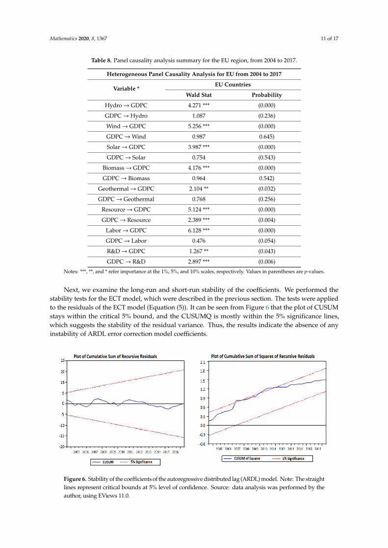
Next, we examine the long-run and short-run stability of the coefficients. We performed thestability tests for the ECT model, which were described in the previous section. The tests were appliedto the residuals of the ECT model (Equation (5)). It can be seen from Figure 6 that the plot of CUSUMstays within the critical 5% bound, and the CUSUMQ is mostly within the 5% significance lines,which suggests the stability of the residual variance. Thus, the results indicate the absence of anyinstability of ARDL error correction model coefficients.

Mathematics 2020, 8, x FOR PEER REVIEW 12 of 18

GDPC → Geothermal 0.768 (0.256) Resource → GDPC 5.124 *** (0.000) GDPC → Resource 2.389 *** (0.004)

Labor → GDPC 6.128 *** (0.000) GDPC → Labor 0.476 (0.054) R&D → GDPC 1.267 ** (0.043) GDPC → R&D 2.897 *** (0.006)

Notes: ***, **, and * refer importance at the 1%, 5%, and 10% scales, respectively. Values in parentheses are p-values.

Next, we examine the long-run and short-run stability of the coefficients. We performed the stability tests for the ECT model, which were described in the previous section. The tests were applied to the residuals of the ECT model (Equation (5)). It can be seen from Figure 6 that the plot of CUSUM stays within the critical 5% bound, and the CUSUMQ is mostly within the 5% significance lines, which suggests the stability of the residual variance. Thus, the results indicate the absence of any instability of ARDL error correction model coefficients.

Figure 6. Stability of the coefficients of the autoregressive distributed lag (ARDL) model. Note: The straight lines represent critical bounds at 5% level of confidence. Source: data analysis was performed by the author, using EViews 11.0.

The Hausman test applied to the regression model analyzing the economic growth at EU level during the period 2004-2017, through the independent variables, led to the results that can be observed in Table 9.

Table 9. Impact of hydro energy, wind energy, solar energy, bioenergy production, geothermal energy, resource productivity, labor force, and R&D development in economic growth, at the EU level.

Correlated Random Effects‒Hausman Test

Test Summary Chi-Square Statistic Chi-Square d.f.* Probability

Cross-section random 10.765397 8 0.0856

Dependent variable Independent variable

Coefficient Prob. R-squared

GDPC Hydro (X1) 0.023 0.045

0.245673 Wind (X2) 0.012 0.008

Figure 6. Stability of the coefficients of the autoregressive distributed lag (ARDL) model. Note: The straightlines represent critical bounds at 5% level of confidence. Source: data analysis was performed by theauthor, using EViews 11.0.

Mathematics 2020, 8, 1367 12 of 17

The Hausman test applied to the regression model analyzing the economic growth at EU levelduring the period 2004-2017, through the independent variables, led to the results that can be observedin Table 9.

Table 9. Impact of hydro energy, wind energy, solar energy, bioenergy production, geothermal energy,resource productivity, labor force, and R&D development in economic growth, at the EU level.

Correlated Random Effects-Hausman Test

Test Summary Chi-Square Statistic Chi-Square d.f. * Probability

Cross-section random 10.765397 8 0.0856

Dependentvariable

Independentvariable Coefficient Prob. R-squared

GDPC

Hydro (X1) 0.023 0.045

0.245673

Wind (X2) 0.012 0.008Solar (X3) 0.007 0.007

Biofuels (X4) 0.153 0.035Geothermal (X5) 0.009 0.003

Resource (X6) 0.125 0.028Labor (X7) 0.237 0.037R&D (X8) 0.205 0.005

Note: * d.f. = degrees of freedom. Source: data analysis was performed by the author, using EViews 11.0.

The results of the panel regression analysis indicate a valid model, while all exogenous variablesare statistically significant. In addition, 24.56% of the variability of the dependent variable is explainedby the variation of the independent variables. The principal result of these quantitative analysesshows that the determinants of renewable energy (hydro, wind, solar, biofuels, and geothermal) aresignificantly relevant for the economic growth, while resource productivity, labor force, and R&Ddevelopment have a positive influence on economic growth, at the European level.

The analysis of the regression coefficients in Table 5 indicates that all renewable energy factorshave a positive and significant impact on economic growth. Thus, a 1 percentage point (pp) increase inprimary hydro energy production leads to an increase of 0.023 pp of GDP per capita. At the same time,a 1 pp increase in primary production of the wind energy leads to a growth of 0.012 pp of GDP percapita, a 1 pp increase in primary solar energy production leads to an increase of 0.007 pp of GDP percapita, a 1 pp increase in primary biofuels production leads to a 0.153 pp increase in GDP per capita,and a 1 pp increase in primary geothermal energy production leads to a growth of 0.009 pp of GDP percapita. Regarding the control factors, we observe that a 1 pp increase in resource productivity leads toa 0.125 pp increase in GDP per capita, while a 1 pp increase in the labor force leads to an increase of0.237 pp. GDP per capita and a 1 pp increase in R&D results in a 0.205 pp increase in GDP per capita.Moreover, RESs and the country-control variables, resource productivity, labor force, and R&D explain24.56% of the economic growth variability.

We next used the Variance Inflection Factor (VIF) test, to test collinearity. The results are shownin Table 10.

Mathematics 2020, 8, 1367 13 of 17

Table 10. The Variance Inflection Factor (VIF) test for collinearity.

Variance Inflation Factors

Date: 10 October 2019 Time: 11:32

Sample: 2004 2017

Included Observations: 392

Variable Coefficient Variance Uncentered VIF Centered VIF

C 5.846 NAHydro 1.475 2.107 1.457Wind 1.598 2.236 1.683Solar 1.162 2.102 1.108

Bioenergy 1.386 2.607 1.783Geothermal 1.902 2.107 1.302

Resource 1.476 2.412 1.403Labor 1.589 2.067 1.355R&D 1.478 1.987 1.201

C = constant. Source: EViews 11.0 output.

In Table 10, we see that the VIF values for all exogenous variables are from 1 to 5. Hence, we couldstate that collinearity issues are not presented in our model.

Thus, we see that all five statistical hypotheses developed at the end of the first section are valid.

5. Discussion and Conclusions

Energy is essential for life, but conventional energy is still the principal source of energy. The mainproblem is that conventional energy causes substantial water and land pollution, and it is alsoresponsible for global warming. As an alternative, renewable energy is limitless, causes less harm forthe environment, and creates new jobs. The present paper uses a panel data random-effects regressionmodel, at the EU level, for the timeframe 2004–2017, and demonstrates that the primary production ofRESs has a statistically significant and positive impact on economic growth. Moreover, it shows thatthe county-level control variables are also significant drivers for economic growth.

The cointegration and ECT models developed with the ARDL model, is applied to the data,in order to determine whether a short-run or a long-run equilibrium relationship exists among economicgrowth and its RES factors. The result indicates that the long-run relationship between the economicgrowth and its factors is stable. In addition, CUSUM and CUSUMSQ tests confirm the stability of theeconomic growth model.

The paper was based on the analysis of a panel data regression model, with economic growth, as anendogenous variable and eight exogenous variables: hydro, wind, solar, biofuels geothermal (renewablefactors), resource, labor, and R&D (control variables). The results reveal that the strongest impact oneconomic growth was that of labor force (coefficient = 0.237), followed by R&D (coefficient = 0.205),biomass (coefficient = 0.153), and productivity of the resources (coefficient = 0.125).

From the econometric analysis, having the economic growth as dependent variable and RES asindependent factors, we get the following regression equation: Y = 0.023X1 + 0.012X2 +0.007X3 +

0.153X4 + 0.009X5 + 0.125X6 + 0.237X7 + 0.205X8.Given that the value of R-squared is 0.2456, we conclude that 24.56% of the variation of the

dependent variable is explained by the independent variables of the model and observe that 75.46% ofthe variance of the endogenous variable is still determined by other factors which are not included inthe study. Moreover, the VIF test reveals that the model does not have collinearity issues.

According to the EU Directive 2009/28/EC, the majority of the EU member states has not yet attainedthe targets set for the consumption of renewable energy for 2020. According to our analysis, only elevenmember states, namely Czech Republic, Bulgaria, Denmark, Croatia, Estonia, Italy, Romania, Lithuania,

Mathematics 2020, 8, 1367 14 of 17

Finland, Hungary, and Sweden, achieved their targets, while only two countries, namely Sweden andFinland, met the 10% target of using renewable energy for the transport sector.

The results of our study validate the conclusions of Reference [58], who made a quantitative analysisto determine the factors of economic growth related to energy and demonstrated that the economicgrowth was partly explained by the levels of R&D, productivity of the resources, and renewable energy.The results are also linked to other research papers [59,60] which state the importance of renewableson economic growth. The authors argue that productivity of the resources and the labor force are twocontrol variables which should be used in the regression model.

In conclusion, we could affirm that the panel data regression model of the economic growth wassignificant and accurately specified and that the structural factors of RESs, i.e., hydro, wind, solar,biomass, and geothermal primary production, as well as the control variables, such as productivity ofthe resources, labor force in RESs, and R&D, were significant factors of the economic growth at the EUlevel. This research paper builds on the recent economic literature dealing with the causality betweenthe renewables and the economic growth, at the EU level [61–68].

Limitations of the study are represented by the timeframe and the number of regressors usedin the econometric model. Future research should analyze the impact of RESs on economic growthby using non-linear models. Moreover, the purchasing power parity will not be overlooked as analternative indicator of the real GDP.

Funding: This research received no external funding.

Acknowledgments: This work was cofinanced by the European Social Fund through Operational ProgramHuman Capital 2014–2020, project number POCU/380/6/13/125015 “Development of entrepreneurial skills fordoctoral students and postdoctoral researchers in the field of economic sciences”.

Conflicts of Interest: The authors declare no conflict of interest.

Abbreviations

EU European UnionEC European CommissionGDP gross domestic productGDPC gross domestic product per capitaR&D research and developmentRES renewable energy systemsEUROSTAT European Union Statistical OfficeOECD Organization for Economic Co-Operation and DevelopmentARDL autoregressive distribution lagVIF Variance Inflection FactorECT error correction termKTOE Kilo ton of oil equivalentCUSUM cumulative sum of the residualsCUSUMQ cumulative sum of squares of the residuals

References

1. Sebri, M. Use renewables to be cleaner: Meta-analysis of the renewable energy consumption-economicgrowth nexus. Renew. Sustain. Energy Rev. 2015, 42, 657–665. [CrossRef]

2. Terrapon-Pfaff, J.; Dienst, C.; Konig, J.; Ortiz, W. A cross-sectional review: Impacts and sustainability ofsmall-scale renewable energy projects in developing countries. Renew. Sustain. Energy Rev. 2014, 40, 1–10.[CrossRef]

3. Bilen, K.; Ozyurt, O.; Bakirci, K.; Karsli, S.; Erdogan, S.; Yimaz, M.; Comakli, O. Energy production,consumption, and environmental pollution for sustainable development: A case study in Turkey.Renew. Sustain. Energy Rev. 2008, 12, 1529–1561. [CrossRef]

4. Gottschamer, L.; Zhang, Q. Interactions of factors impacting implementation and sustainability of renewableenergy sourced electricity. Renew. Sustain. Energy Rev. 2016, 65, 164–174. [CrossRef]

Mathematics 2020, 8, 1367 15 of 17

5. U.S. Energy Information Administration. International Energy Outlook 2016; U.S. Energy InformationAdministration: Washington, DC, USA, 2016.

6. Vaona, A. The effect of renewable energy generation on import demand. Renew. Energy 2016, 86, 354–359.[CrossRef]

7. Alper, A.; Oguz, O. The role of renewable energy consumption in economic growth: Evidence fromasymmetric causality. Renew. Sustain. Energy Rev. 2016, 60, 953–959. [CrossRef]

8. Menegaki, A.N. Growth and renewable energy in Europe: A random effect model with evidence for neutralityhypothesis. Energy Econ. 2011, 33, 257–263. [CrossRef]

9. Beça, P.; Santos, R. Measuring sustainable welfare: A new approach to the isew. Ecol. Econ. 2010, 69, 810–819.[CrossRef]

10. Moldan, B.; Janouskova, S.; Hak, T. How to understand and measure environmental sustainability: Indicatorsand targets. Ecol. Indic. 2012, 17, 4–13. [CrossRef]

11. Menegaki, A.N.; Tugcu, C.T. Energy consumption and sustainable economic welfare in G7 countries;A comparison with the conventional nexus. Renew. Sustain. Energy Rev. 2017, 69, 892–901. [CrossRef]

12. Vasylieva, T.; Lyulyov, O.; Bilan, Y.; Streimikiene, D. Sustainable economic development and greenhouse gasemissions: The dynamic impact of renewable energy consumption, GDP, and corruption. Energies 2019, 12,3289. [CrossRef]

13. D’Adamo, I.; Rosa, P. A structured literature review on obsolete electric vehicles management practices.Sustainability 2019, 11, 6876. [CrossRef]

14. D’Adamo, I.; Falcone, P.M.; Gastaldi, M.; Morone, P. RES-T trajectories and an integrated SWOT-AHP analysisfor biomethane. Policy implications to support a green revolution in European transport. Energy Policy 2020,138, 111220. [CrossRef]

15. Gilpin, R.; Gilpin, J.M. Global Political Economy: Understanding the International Economic Order; PrincetonUniversity Press: Princeton, NJ, USA, 2011.

16. Busu, M. Assessment of the Impact of Bioenergy on Sustainable Economic Development. Energies 2019, 12,578. [CrossRef]

17. European Union. Directive 2009/28/EC of the European parliament and of the council of 23 April 2009 on thepromotion of the use of energy from renewable sources and amending and subsequently repealing directives2001/77/EC and 2003/30/EC (text with EEA relevance). Off. J. Eur. Union 2009, 5, 2009.

18. Eurostat. Available online: http://ec.europa.eu/eurostat (accessed on 30 June 2019).19. Bhattacharya, M.; Paramati, S.R.; Ozturk, I.; Bhattacharya, S. The effect of renewable energy consumption on

economic growth: Evidence from top 38 countries. Appl. Energy 2016, 162, 733–741. [CrossRef]20. Inglesi-Lotz, R. The impact of renewable energy consumption to economic growth: A panel data application.

Energy Econ. 2016, 53, 58–63. [CrossRef]21. Huang, B.N.; Hwang, M.J.; Yang, C.W. Causal relationship between energy consumption and GDP growth

revisited: A dynamic panel data approach. Ecol. Econ. 2008, 67, 41–54. [CrossRef]22. Shahbaz, M.; Rasool, G.; Ahmed, K.; Mahalik, M.K. Considering the effect of biomass energy consumption

on economic growth: Fresh evidence from BRICS region. Renew. Sustain. Energy Rev. 2016, 60, 1442–1450.[CrossRef]

23. Sadorsky, P. Renewable energy consumption, CO2 emissions and oil prices in the G7 countries. Energy Econ.2009, 31, 456–462. [CrossRef]

24. Guzowski, C.; Recalde, M. Latin American electricity markets and renewable energy sources: The Argentineanand Chilean cases. Int. J. Hydrog. Energy 2010, 35, 5813–5817. [CrossRef]

25. Lee, C.C.; Chen, S.T. Do defence expenditures spur GDP? A panel analysis from OECD and non-OECDcountries. Def. Peace Econ. 2007, 18, 265–280. [CrossRef]

26. Apergis, N.; Payne, J.E. The renewable energy consumption–growth nexus in Central America. Appl. Energy2011, 88, 343–347. [CrossRef]

27. Apergis, N.; Salim, R. Renewable energy consumption and unemployment: Evidence from a sample of 80countries and nonlinear estimates. Appl. Econ. 2015, 47, 5614–5633. [CrossRef]

28. Sebri, M.; Ben-Salha, O. On the causal dynamics between economic growth, renewable energy consumption,CO2 emissions and trade openness: Fresh evidence from BRICS countries. Renew. Sustain. Energy Rev. 2014,39, 14–23. [CrossRef]

Mathematics 2020, 8, 1367 16 of 17

29. Koçak, E.; Sarkgünesi, A. The renewable energy and economic growth nexus in black sea and Balkancountries. Energy Policy 2017, 100, 51–57. [CrossRef]

30. Amri, F. Intercourse across economic growth, trade and renewable energy consumption in developing anddeveloped countries. Renew. Sustain. Energy Rev. 2017, 69, 527–534. [CrossRef]

31. Ocal, O.; Aslan, A. Renewable energy consumption-economic growth nexus in Turkey. Renew. Sustain. Energy Rev.2013, 28, 494–499. [CrossRef]

32. Tiwari, A.K. A structural VAR analysis of renewable energy consumption, real GDP and CO2 emissions:Evidence from India. Econ. Bull. 2011, 31, 1793–1806.

33. Mansouri, N.; Lashab, A.; Sera, D.; Guerrero, J.M.; Cherif, A. Large Photovoltaic Power Plants Integration:A Review of Challenges and Solutions. Energies 2019, 12, 3798. [CrossRef]

34. Babatunde, O.M.; Munda, J.L.; Hamam, Y. Selection of a Hybrid Renewable Energy Systems for a Low-IncomeHousehold. Sustainability 2019, 11, 4282. [CrossRef]

35. Moncada-Paternò-Castello, P.; Ciupagea, C.; Smith, K.; Tübke, A.; Tubbs, M. Does Europe perform too littlecorporate R&D? A comparison of EU and non-EU corporate R&D performance. Res. Policy 2010, 39, 523–536.

36. Bai, J.; Ding, T.; Wang, Z.; Chen, J. Day-Ahead Robust Economic Dispatch Considering Renewable Energyand Concentrated Solar Power Plants. Energies 2019, 12, 3832. [CrossRef]

37. Xu, L.; Wang, Y.; Solangi, Y.A.; Zameer, H.; Shah, S.A.A. Off-Grid Solar PV Power Generation System inSindh, Pakistan: A Techno-Economic Feasibility Analysis. Processes 2019, 7, 308. [CrossRef]

38. Alhamid, M.I.; Daud, Y.; Surachman, A.; Sugiyono, A.; Aditya, H.B.; Mahlia, T.M.I. Potential of geothermalenergy for electricity generation in Indonesia: A review. Renew. Sustain. Energy Rev. 2016, 53, 733–740.

39. Mathiesen, B.V.; Lund, H.; Connolly, D.; Wenzel, H.; Østergaard, P.A.; Möller, B.; Nielsen, S.; Ridjan, I.;Karnøe, P.; Sperling, K.; et al. Smart Energy Systems for coherent 100% renewable energy and transportsolutions. Appl. Energy 2015, 145, 139–154. [CrossRef]

40. Busu, M. Applications of TQM Processes to Increase the Management Performance of Enterprises in theRomanian Renewable Energy Sector. Processes 2019, 7, 685. [CrossRef]

41. Pelau, C.; Acatrinei, C. The Paradox of Energy Consumption Decrease in the Transition Period towards aDigital Society. Energies 2019, 12, 1428. [CrossRef]

42. Siddaiah, R.; Saini, R.P. A review on planning, configurations, modeling and optimization techniques ofhybrid renewable energy systems for off grid applications. Renew. Sustain. Energy Rev. 2016, 58, 376–396.[CrossRef]

43. D’Adamo, I.; Rosa, P. How Do You See Infrastructure? Green Energy to Provide Economic Growth afterCOVID-19. Sustainability 2020, 12, 4738. [CrossRef]

44. Elmqvist, T.; Andersson, E.; Frantzeskaki, N.; McPhearson, T.; Olsson, P.; Gaffney, O.; Takeuchi, K.; Folke, C.Sustainability and resilience for transformation in the urban century. Nat. Sustain. 2019, 2, 267–273.[CrossRef]

45. Johansen, S. Statistical analysis of cointegration vectors. J. Econ. Dyn. Control 1998, 12, 231–254. [CrossRef]46. Johansen, S.; Juselius, K. Maximum likelihood estimation and inference on cointegration—With applications

to the demand for money. Oxf. Bull. Econ. Stat. 1990, 52, 169–210. [CrossRef]47. Pesaran, M.H.; Shin, Y. Autoregressive Distributed Lag Modelling Approach to Cointegration Analysis; DAE

Working Paper Series No. 9514; Department of Applied Economics, University of Cambridge: Cambridge,UK, 1995.

48. Sulaiman, C.; Abdul-Rahim, A.S. Population Growth and CO2 Emission in Nigeria: A Recursive ARDLApproach. SAGE Open 2018, 2, 215824401876591. [CrossRef]

49. Sulaiman, C.; Bala, U.; Tijani, B.A.; Ibrahim Waziri, S.I.; Maji, I.K. Human Capital, Technology, and EconomicGrowth: Evidence from Nigeria. SAGE Open 2015, 5, 2158244015615166. [CrossRef]

50. Sheng, P.; Guo, X. The Long-run and Short-run Impacts of Urbanization on Carbon Dioxide Emissions.Econ. Model. 2016, 53, 208–215. [CrossRef]

51. Narayan, P.K. Reformulating Critical Values for the Bounds F-Statistics Approach to Cointegration: An Application tothe Tourism Demand Model for Fiji; Department of Economics Discussion Papers No. 02/04; Monash University:Melbourne, Australia, 2004.

52. Narayan, P.K.; Narayan, S. Estimating income and price elasticities of imports for Fiji in a cointegrationframework. Econ. Model. 2005, 22, 423–438. [CrossRef]

Mathematics 2020, 8, 1367 17 of 17

53. Narayan, P.K.; Smyth, R. Temporal causality and the dynamics of exports, human capital and real income inChina. Int. J. Appl. Econ. 2004, 1, 24–45.

54. Pesaran, M.H.; Shin, Y.; Smith, R.J. Bounds testing approaches to the analysis of level relationships.J. Appl. Econom. 2001, 16, 289–326. [CrossRef]

55. Yitzhaki, S. Gini’s mean difference: A superior measure of variability for non-normal distributions. Metron2003, 61, 285–316.

56. Dabholkar, P.A.; Shepherd, C.D.; Thorpe, D.I. A comprehensive framework for service quality:An investigation of critical conceptual and measurement issues through a longitudinal study. J. Retail. 2000,76, 139–173. [CrossRef]

57. Evans, A.; Strezov, V.; Evans, T.J. Sustainability considerations for electricity generation from biomass.Renew. Sustain. Energy Rev. 2010, 14, 1419–1427. [CrossRef]

58. Busu, M. The Role of Renewables in a Low-Carbon Society: Evidence from a Multivariate Panel DataAnalysis at the EU Level. Sustainability 2019, 11, 5260. [CrossRef]

59. Xie, J.; Saltzman, S. Environmental policy analysis: An environmental computable general-equilibriumapproach for developing countries. J. Policy Model. 2000, 22, 453–489. [CrossRef]

60. Aarstad, J.; Kvitastein, O.A.; Jakobsen, S.E. Related and unrelated variety as regional drivers of enterpriseproductivity and innovation: A multilevel study. Res. Policy 2016, 45, 844–856. [CrossRef]

61. Destek, M.A.; Aslan, A. Renewable and non-renewable energy consumption and economic growth inemerging economies: Evidence from bootstrap panel causality. Renew. Energy 2017, 111, 757–763. [CrossRef]

62. Irandoust, M. The renewable energy-growth nexus with carbon emissions and technological innovation:Evidence from the Nordic countries. Ecol. Indic. 2016, 69, 118–125. [CrossRef]

63. Uniejewski, B.; Weron, R. Efficient Forecasting of Electricity Spot Prices with Expert and LASSO Models.Energies 2018, 11, 2039. [CrossRef]

64. Gianfreda, A.; Parisio, L.; Pelagatti, M. Revisiting long-run relations in power markets with high RESpenetration. Energy Policy 2016, 94, 432–445. [CrossRef]

65. Pelau, C.; Pop, N.A. Implications for the energy policy derived from the relation between the culturaldimensions of Hofstede’s model and the consumption of renewable energies. Energy Policy 2018, 118, 160–168.[CrossRef]

66. Saad, W.; Taleb, A. The causal relationship between renewable energy consumption and economic growth:Evidence from Europe. Clean Technol. Environ. Policy 2018, 20, 127–136. [CrossRef]

67. Bunn, D.; Gianfreda, A.; Kermer, S. A trading-based evaluation of density forecasts in a real-time electricitymarket. Energies 2018, 11, 2658. [CrossRef]

68. Busu, M.; Trica, C.L. Sustainability of Circular Economy Indicators and Their Impact on Economic Growth ofthe European Union. Sustainability 2019, 11, 5481. [CrossRef]

© 2020 by the author. Licensee MDPI, Basel, Switzerland. This article is an open accessarticle distributed under the terms and conditions of the Creative Commons Attribution(CC BY) license (http://creativecommons.org/licenses/by/4.0/).