Rochester Institute of Technology Rochester Institute of Technology

RIT Scholar Works RIT Scholar Works

Theses

11-2020

Analyzing the Impact of Negative Sampling on Fact-Prediction Analyzing the Impact of Negative Sampling on Fact-Prediction

Algorithms Algorithms

Iti Bansal ib6355@rit.edu

Follow this and additional works at: https://scholarworks.rit.edu/theses

Recommended Citation Recommended Citation Bansal, Iti, "Analyzing the Impact of Negative Sampling on Fact-Prediction Algorithms" (2020). Thesis. Rochester Institute of Technology. Accessed from

This Thesis is brought to you for free and open access by RIT Scholar Works. It has been accepted for inclusion in Theses by an authorized administrator of RIT Scholar Works. For more information, please contact ritscholarworks@rit.edu.

Analyzing the Impact of NegativeSampling on

Fact-Prediction Algorithms

by

Iti Bansal

A Thesis Submittedin

Partial Fulfillment of theRequirements for the Degree of

Master of Sciencein

Computer Science

Supervised by

Dr. Carlos R. Rivero

Department of Computer Science

B. Thomas Golisano College of Computing and Information SciencesRochester Institute of Technology

Rochester, New York

November 2020

ii

The thesis “Analyzing the Impact of Negative Sampling on

Fact-Prediction Algorithms” by Iti Bansal has been examined and approved by the follow-

ing Examination Committee:

Dr. Carlos R. RiveroAssistant ProfessorThesis Committee Chair

Dr. Zack ButlerProfessor

Dr. Ifeoma NwoguAssistant Professor

iii

Acknowledgments

I would like to express my sincere gratitude towards my advisor Dr. Carlos R. Rivero for

his guidance throughout this work. I am grateful to him for giving me an opportunity to

collaborate on his research work. His teachings have been very critical to me to build a

strong foundation in the area of knowledge graphs. I am thankful to Dr. Zack Butler and

Dr. Ifeoma Nwogu for serving on my committee and giving me constructive feedback on

my work.

I would like to give my regards to my parents Rajendra K. Bansal and Seema Bansal for

constantly encouraging me to pursue challenging work. Finally, I would like to thank my

siblings Mansi Bansal and Sarvagya Bansal, and my friends who have been a great support

throughout this work.

iv

Abstract

Analyzing the Impact of Negative Sampling onFact-Prediction Algorithms

Iti Bansal

Superviser: Dr. Carlos R. Rivero

Knowledge graphs are useful for many applications like product recommendations and

web search query engines. However, knowledge graphs are marked by incompleteness.

Fact-prediction algorithms aim to expand knowledge graphs by predicting missing facts.

Fact-prediction algorithms train models using positive facts present and creating negative

facts not present in the knowledge graph at hand. Negative facts are obtained by corrupt-

ing information in the positive facts present in the knowledge graph at hand. Although it

is generally assumed that negative facts drive the accuracy of fact-prediction algorithms,

this concept has not been thoroughly examined yet. In this work, we investigate whether

negative facts indeed drive fact-prediction accuracy by employing different negative fact

generation strategies in translation-based algorithms, a popular branch of fact-prediction

algorithms. We propose a new negative fact generation strategy that utilizes knowledge

from immediate neighbors to corrupt a fact. Our extensive experiments using well-known

benchmarking datasets show that negative facts indeed drive the accuracy of fact-prediction

models, and that this accuracy dramatically changes depending on the negative fact gen-

eration strategy used for training and testing models. Assuming that the strategies gen-

erate negative facts with different levels of semantic plausibility, we observe that models

v

trained using certain strategies are not able to distinguish missing facts from nonsensical

or semantically-related facts. Additionally, our results show that the accuracy of models

trained using the local-closed world assumption, the most common negative fact genera-

tion strategy, can be achieved with a combination of neighborhood-based and nonsensical

strategies. This implies that fact-prediction algorithms can be trained using individual sub-

graphs instead of the whole knowledge graph, opening new research avenues.

vi

Contents

Acknowledgments . . . . . . . . . . . . . . . . . . . . . . . . . . . . . . . . . iii

Abstract . . . . . . . . . . . . . . . . . . . . . . . . . . . . . . . . . . . . . . . iv

1 Introduction . . . . . . . . . . . . . . . . . . . . . . . . . . . . . . . . . . . 11.1 Problem Statement . . . . . . . . . . . . . . . . . . . . . . . . . . . . . . 21.2 Plan of work . . . . . . . . . . . . . . . . . . . . . . . . . . . . . . . . . . 21.3 Summary of Results . . . . . . . . . . . . . . . . . . . . . . . . . . . . . . 3

2 Background . . . . . . . . . . . . . . . . . . . . . . . . . . . . . . . . . . . 52.1 Knowledge Graphs . . . . . . . . . . . . . . . . . . . . . . . . . . . . . . 52.2 Machine Learning in Knowledge Graphs . . . . . . . . . . . . . . . . . . . 72.3 Knowledge Graph Refinement . . . . . . . . . . . . . . . . . . . . . . . . 8

2.3.1 Knowledge Graph Embedding . . . . . . . . . . . . . . . . . . . . 92.3.2 Translation-Based Models . . . . . . . . . . . . . . . . . . . . . . 10

3 Generating Negative Facts . . . . . . . . . . . . . . . . . . . . . . . . . . . 153.1 Naıve . . . . . . . . . . . . . . . . . . . . . . . . . . . . . . . . . . . . . 163.2 Local-Closed World Assumption (LCWA) . . . . . . . . . . . . . . . . . . 173.3 Typed Local-Closed World Assumption (TLCWA) . . . . . . . . . . . . . 173.4 Neighborhood-based Local-Closed World Assumption (NLCWA) . . . . . 19

4 Fact-prediction implementation . . . . . . . . . . . . . . . . . . . . . . . . 214.1 Fact-prediction workflow . . . . . . . . . . . . . . . . . . . . . . . . . . . 214.2 OpenKE . . . . . . . . . . . . . . . . . . . . . . . . . . . . . . . . . . . . 23

5 Experiments . . . . . . . . . . . . . . . . . . . . . . . . . . . . . . . . . . . 265.1 Experiment Setup . . . . . . . . . . . . . . . . . . . . . . . . . . . . . . . 265.2 Anomalies . . . . . . . . . . . . . . . . . . . . . . . . . . . . . . . . . . . 275.3 Datasets . . . . . . . . . . . . . . . . . . . . . . . . . . . . . . . . . . . . 28

vii

5.4 Evaluation metrics . . . . . . . . . . . . . . . . . . . . . . . . . . . . . . 305.5 Results . . . . . . . . . . . . . . . . . . . . . . . . . . . . . . . . . . . . . 33

6 Conclusions . . . . . . . . . . . . . . . . . . . . . . . . . . . . . . . . . . . 376.1 Conclusion . . . . . . . . . . . . . . . . . . . . . . . . . . . . . . . . . . 376.2 Future Work . . . . . . . . . . . . . . . . . . . . . . . . . . . . . . . . . . 37

Bibliography . . . . . . . . . . . . . . . . . . . . . . . . . . . . . . . . . . . . 39

A Code Listing . . . . . . . . . . . . . . . . . . . . . . . . . . . . . . . . . . 44A.1 Python code to generate negative facts . . . . . . . . . . . . . . . . . . . . 44

viii

List of Tables

5.1 Knowledge graphs under evaluation . . . . . . . . . . . . . . . . . . . . . 295.2 Example of ranking Criterion . . . . . . . . . . . . . . . . . . . . . . . . . 325.3 Training with naıve . . . . . . . . . . . . . . . . . . . . . . . . . . . . . . 345.4 Training with LCWA . . . . . . . . . . . . . . . . . . . . . . . . . . . . . 345.5 Training with TLCWA . . . . . . . . . . . . . . . . . . . . . . . . . . . . 355.6 Training with NLCWA . . . . . . . . . . . . . . . . . . . . . . . . . . . . 355.7 Training with naıve + NLCWA . . . . . . . . . . . . . . . . . . . . . . . . 36

ix

List of Figures

2.1 Soccer players with their country of birth, team and country of team . . . . 62.2 Vector representation of a positive fact learned by TransE [6] . . . . . . . . 112.3 Vector representation of a negative fact learned by TransE . . . . . . . . . . 112.4 Vector representation of a fact in TransH (adpated from [34]) . . . . . . . . 122.5 Vector representation of a fact in TransR (adapted from [21]) . . . . . . . . 13

4.1 Workflow of training and testing fact-prediction models . . . . . . . . . . . 21

1

Chapter 1

Introduction

Knowledge graphs are an important source for information retrieval applications like web

search engines and social network analysis [15]. In a knowledge graph, nodes and edges

are stored in the form of triples (h, r, t), where h and t are the head and tail entities, and

r is a relation. For example, a fact about New York state’s capital can be represented as

(New York, HasCapital, Albany) where New York and Albany are entities and HasCap-

ital is a relation. Knowledge graphs are often drawn from open data sources like Wiki-

data and DBpedia [2, 31] and refined using methods like natural language processing [35].

Knowledge graphs are generally constructed with minimal or no human supervision [5].

Even though there have been many advances in their unsupervised construction, there are

vast amounts of knowledge that is difficult to acquire [5]. This leads to incompleteness

in knowledge graphs, i.e., there are missing facts or edges [36]. To overcome this is-

sue, fact-prediction algorithms determine missing relations between existing entities in the

knowledge graph [24].

In this study, we focus on translation-based models, a branch of fact-prediction models

that measures the plausibility of a missing fact. Translation-based models utilize negative

facts to train and test a fact-prediction model [6, 34, 17]. For each positive fact in the

training set, TransE, one of the most popular algorithms in this context, corrupts either the

head or the tail (one at a time) by replacing it with a random entity, such that the resulting

fact is not present in the knowledge graph [6]. However, under the open-world assumption

in which a missing fact is not negative but unknown, it is challenging to generate negative

facts that are truly incorrect since they may be correct but missing. To generate negative

2

facts, the most popular strategy is the local-closed world assumption (LCWA) [], in which,

for a given relation, if there exists at least one value for the related entities, then it contains

all possible values for those entities for that relation [16, 9, 12]. Recently, other strategies

have been proposed that use prior knowledge in the form of type constraints to generate

semantically-related negative facts [16, 19]. However, knowledge graphs often suffer from

type incompleteness, so it is difficult to employ such strategies for fact-prediction [7].

1.1 Problem Statement

Translation-based models require a set of negative facts for the prediction of new facts. In

the training phase, one negative fact is created per positive fact; in the test phase, all possible

negative facts are created per positive fact. The accuracy of fact-checking algorithms is

assumed to be driven by the negative facts used during training [6]. However, this idea has

not been thoroughly examined yet. In this research, we are trying to answer the following

questions:

1. Will the accuracy of fact-prediction algorithms vary with strategies other than the

local-closed world assumption?

2. Will the accuracy of fact-prediction algorithms differ with the expected semantic

plausibility of negative facts generated by each strategy?

1.2 Plan of work

We propose to study the impact of negative sampling by experimenting with different neg-

ative fact generation strategies on a variety of datasets like Freebase [4], Wordnet [11],

Yet Another Great Ontology (YAGO) [22], and Never-Ending Language Learning (NELL)

[23]. These strategies differ in the way candidates are selected from the knowledge graph

for corruption. Unlike local-closed world assumption, we strictly select entities associated

with the input relation of the triple at hand for corruption, which is supposed to give more

3

semantically plausible negative facts. We further extend this strategy to look into the neigh-

borhood for possible candidates for corruption. For evaluating the model, the facts in the

test set are ranked against their negative counterparts. An accurate model ranks positive

facts higher than their negative counterparts.

1.3 Summary of Results

We evaluate translation-based models: TransE [6], TransH [34], and TransD [17] with four

different negative fact generation strategies: naıve [18], local-closed world assumption

(LCWA) [18], typed local-closed world assumption (TLCWA) [18], and neighborhood-

based local-closed world assumption (NLCWA). NLCWA is a new strategy developed by

us in extension to TLCWA. While naıve is expected to generate mainly nonsensical facts,

LCWA, TLCWA, and NLCWA generate a combination of nonsensical facts and semanti-

cally plausible facts. LCWA utilizes the entire knowledge graph to generate negative facts,

therefore it is expected to generate more nonsensical facts than semantically plausible. Due

to the more restrictive nature of TLCWA, it is bound to generate essentially semantically

plausible facts. On the other hand, NLCWA produces additional negative facts not cov-

ered by TLCWA that are expected to be semantically plausible. Let NL, NT , and NN

denote the true negative facts generated by LCWA, TLCWA, and NLCWA respectively,

then NT ⊆ NN ⊆ NL.

Our results show that the accuracy of the models varies with different strategies used.

To make this impact explicit, we fix one strategy at a time for training and test using all the

four strategies. When a model is trained and tested using the naıve strategy, the accuracy of

the model is high. However, the accuracy drops when trained using naıve and tested with

the other three strategies. We believe this is because naıve is expected to generate more of

nonsensical facts and, hence, cannot recognize semantically plausible facts examined by

other strategies.

A model trained with LCWA has lower accuracy when tested with naıve and better

accuracy when tested with TLCWA and NLCWA. This is because LCWA generates all

4

possible facts, including nonsensical and semantically plausible. A model trained with

TLCWA has the worst accuracy when tested with naıve and LCWA as it is too restrictive

since TLCWA generates the most semantically plausible facts. However, a model trained

using TLCWA but tested with TLCWA and NLCWA shows a fair accuracy as the negative

facts are semantically plausible. A model trained with NLCWA has comparable accuracy

to the model trained with LCWA except when tested with the naive strategy, where we

observe a lower accuracy. We further investigate the behavior of NLCWA such that we

train a model with a combination of naıve and NLCWA to benefit from both strategies.

This model outperforms the accuracy of all models except in the case of one dataset.

We observe that the accuracy of the model fluctuates w.r.t. to the strategy used for

training and testing. If a model is trained with a strategy that generates largely nonsensi-

cal negative facts, the model fails to recognize semantically plausible facts. Whereas, if

a model is trained with a strategy that generates mainly semantically plausible facts, the

model cannot distinguish the nonsensical facts. A model trained with a strategy that gener-

ates a combination of nonsensical and semantically plausible negative facts performs fairly

with all types of facts.

5

Chapter 2

Background

In this chapter, we give an introduction about knowledge graphs and knowledge graph re-

finement techniques. Section 2.1 explains the representation of the knowledge graph with

the help of an example, knowledge graph creation techniques using external sources, and

the use of graph databases to store knowledge graphs. Section 2.2 discusses how to apply

machine learning algorithms particularly stochastic gradient descent on knowledge graphs.

Section 2.3 presents knowledge graph refinement techniques using knowledge graph em-

beddings. We particularly focus our attention on translational-based models [6, 34].

2.1 Knowledge Graphs

A knowledge graph is a network of data represented by a graph, where entities are nodes

in the graph and relations are edges between the entities [15]. Figure 2.1 depicts an ex-

ample of a graph representing information about soccer players extracted from DBpedia,

a popular knowledge graph based on Wikipedia [2]. The soccer players (Juan Olave, Juan

Pablo Carrizo, Leo France, William Peterson, Dario Sala, Emiliano Martinez), teams (Club

Bolivar, Real Zaragoza, Club Altetico Independiente), and countries (Argentina, Bolivia,

Spain, United Kingdom) are entities, and the team of a player (team), country of birth

(countryOfBirth), and country of the team (countryOfTeam) are the relations in the graph.

The relations in the graph are shown as directed, black-solid arrows.

Knowledge graphs are built from multiple sources of data covering human contribu-

tions, text corpus on websites, CSV files, and relational databases within organizations

6

[5]. Semi-supervised or unsupervised methods are used to extract information from these

sources as it is very expensive to have a completely supervised method. The constructed

knowledge graph may have discrepancies due to errors in the extraction process, ambi-

guity, or noise in the data [5]. Hence, knowledge graphs are marked by incompleteness

and inconsistencies. In Figure 2.1, red-dotted arrows represent the missing relations in the

knowledge graph.

Knowledge graphs are stored in graph databases that have several advantages over rela-

tional and non-relational databases [15, 26]. Graph databases do not require the existence

of a well-defined schema, giving it the flexibility to handle missing information. Along

with relational operators like joins, unions, and projections, navigational operators pro-

vide a way to reach entities that are connected through an unpredictable number of edges.

Graph databases give the flexibility to store, maintain, and model data in many domains

like social, biological, and web networks [26].

Figure 2.1: Soccer players with their country of birth, team and country of team

7

2.2 Machine Learning in Knowledge Graphs

Machine learning is used to detect and extrapolate meaningful patterns in data [3]. Knowl-

edge graphs utilize machine learning algorithms to infer new facts from the existing facts

[3]. The traditional machine learning model extracts features from the data and maps pa-

rameters to the desired output. For example, in an image classification problem, a convo-

lution neural network (CNN) receives images as input to determine the class of image, i.e.,

the output. The weights of the CNN are the parameters that can be learned from the data

and used to make prediction.

Machine learning applied to knowledge graphs takes facts as input, where each fact is

represented by an edge (relation) between two nodes (entities) in a knowledge graph, and

learns embeddings of entities and relations. The embeddings are analogous to the weights

of CNN in image classification problem and are thus the parameters of the fact-prediction

model. The embeddings are useful for various machine learning tasks like predicting miss-

ing edges, predicting the property of nodes, and clustering nodes based on similarity [32].

Gradient descent is one of the most popular machine learning algorithm used to learn em-

beddings in knowledge graphs.

Algorithm 1: Stochastic Gradient DescentInput: training set, maxepochs, batch size , loss function, params, learning rate

1 for i in range(maxepochs) do

2 mini batch← sample random batch(training set, batch size) ;

3 params grad← evaluate gradient(loss function, mini batch , params) ;

4 params← params - learning rate * params grad

5 end

The objective of gradient descent is to learn model parameters (embeddings in the case

of knowledge graphs) by minimizing a cost function that evaluates the performance of the

model. Vanilla gradient descent or batch gradient descent [27] uses the whole training set

8

to compute the gradient of the cost function with respect to the model parameters until

convergence. When the training set is large, batch gradient descent is computationally

expensive since it uses the whole set. To improve performance, stochastic gradient descent

[27] picks one random training example per iteration to update model parameters based

on gradients. The frequent updates of parameters cause the cost function to fluctuate from

one local minimum to another. While stochastic gradient descent runs faster than vanilla

gradient descent, it leads to unstable convergence.

Mini-batch gradient descent is a variant of stochastic gradient descent in which, instead

of a computing gradient on a single sample, it is computed over a mini-batch sampled

from the training set. This stabilizes the fluctuations in stochastic gradient descent and

leads to stable convergence. Most of the fact-prediction algorithms use stochastic gradient

descent in mini-batch mode to train a model [32], which we present in Algorithm 1. For a

predetermined number of epochs, a random batch of fixed size is sampled from the training

set. For each parameter, the gradient of the loss function is computed for the sampled batch.

Parameters are updated w.r.t a learning rate, i.e., a hyperparameter to decide how large the

update should be [27].

2.3 Knowledge Graph Refinement

Knowledge graphs are created by collating information from various sources such as hu-

man editors, text sources, and structured sources [15]. Information from human editors

is collected through crowd-sourcing platforms, customer feedback forms, and open-source

editing tools like Wikipedia. While incurring direct contributions from humans can be ex-

pensive, it can be inaccurate due to human error, and differences in opinion. Text present

in news articles, social media posts, and scientific publications are extracted using an un-

supervised technique like Natural Language Processing (NLP) [15]. NLP decides which

words to include in the facts, sometimes eliminating crucial information from the relation

phrase [5]. Thus, it is not possible to have fully complete or correct knowledge graphs

due to the limitations of the information-extraction methods. To address this issue, various

9

knowledge graph completion and correctness methods have been proposed [24].

A knowledge graph is completed by finding missing entities, missing relations or facts,

or missing types [24]. Knowledge graph refinement refers to the use of existing facts to add

missing facts or remove erroneous facts from the knowledge graph [24]. Whereas comple-

tion may involve the use of external sources to find the missing entities and types [24].

We focus our analysis on fact-prediction algorithms that refine knowledge graphs by iden-

tifying missing facts. A fact-prediction algorithm predicts the probability of correctness

of missing facts [6, 34]. For example, in Figure 2.1, the information about the country of

birth for the players Leo France and Emiliano Martinez is missing, which is represented by

red-dotted arrows. To check if Leo France and Emiliano Martinez are born in Argentina,

we rank the facts (Leo France countryOfBirth Argentina) and (Emiliano Martinez country-

OfBirth Argentina) against the corresponding negative facts derived from them. The ranks

are determined based on the plausibility scores assigned to the facts that are drawn based

on the connections of entities involved in the facts with surrounding entities.

A knowledge graph is corrected by identifying and removing incorrect facts using fact-

validation. Fact-validation refers to assigning a plausibility score to the existing facts and

subsequently ranking them in the decreasing order of the scores [6, 34]. For example,

in Figure 2.1, most of the players have their country of birth different from the country of

their teams. Although these are true facts, correctness of these facts can be verified by using

fact-validation. Fact-prediction and fact-validation are related as both depend on estimating

the probability of facts to refine a knowledge graph. In the following sections, we discuss

knowledge graph embeddings and fact-prediction algorithms based on translation-based

embeddings [6].

2.3.1 Knowledge Graph Embedding

Knowledge graphs are stored in the form of triples representing edges as (h, r, t), where h

is a head entity, r is a relation and t is a tail entity. To capture dependency between entities,

entities and relations are embedded into continuous vector spaces [32]. The embeddings

10

are randomly initialized at the beginning and are manipulated based on the requirement

of specific machine learning algorithm. Several algorithms just utilize facts present in the

knowledge graph at hand, i.e., the relations among entities for learning the embeddings

[6, 34], while others take additional information like entity types [13, 37], relation paths

[20, 30], and textual descriptions [33, 38] into account.

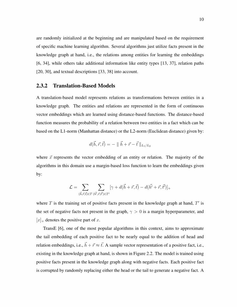
2.3.2 Translation-Based Models

A translation-based model represents relations as transformations between entities in a

knowledge graph. The entities and relations are represented in the form of continuous

vector embeddings which are learned using distance-based functions. The distance-based

function measures the probability of a relation between two entities in a fact which can be

based on the L1-norm (Manhattan distance) or the L2-norm (Euclidean distance) given by:

d(~h, ~r,~t) = − ‖ ~h+ ~r − ~t ‖L1/L2

where ~x represents the vector embedding of an entity or relation. The majority of the

algorithms in this domain use a margin-based loss function to learn the embeddings given

by:

L =∑

(~h,~r,~t)∈T

∑(~h′,~r,~t′)∈T ′

[γ + d(~h+ ~r,~t)− d(~h′ + ~r, ~t′)]+

where T is the training set of positive facts present in the knowledge graph at hand, T ′ is

the set of negative facts not present in the graph, γ > 0 is a margin hyperparameter, and

[x]+ denotes the positive part of x.

TransE [6], one of the most popular algorithms in this context, aims to approximate

the tail embedding of each positive fact to be nearly equal to the addition of head and

relation embeddings, i.e., ~h+ ~r ≈ ~t. A sample vector representation of a positive fact, i.e.,

existing in the knowledge graph at hand, is shown in Figure 2.2. The model is trained using

positive facts present in the knowledge graph along with negative facts. Each positive fact

is corrupted by randomly replacing either the head or the tail to generate a negative fact. A

11

sample vector representation of a negative fact derived from a positive fact with corrupted

tail is shown in Figure 2.3.

Figure 2.2: Vector representation of apositive fact learned by TransE [6]

Figure 2.3: Vector representation of anegative fact learned by TransE

Algorithm 2: TransEInput: Training set T , entity set E, relation set R, margin γ, embeddings

dimension k

1 ~e← vector of k × 1 for each e ∈ E ;

2 ~r ← vector of k × 1 for each r ∈ R ;

3 ~r ← ~r/ ‖ ~r ‖ for each r ∈ R ;

4 Loop

5 ~e← ~e/ ‖ ~e ‖ for each e ∈ E ;

6 S ← sample a subset from T ;

7 B ← {} ;

8 for (h, r, t) ∈ S do

9 (h′, r, t′)← corrupt((h, r, t));

10 B ← B ∪ {(h, r, t), (h′, r, t′)}

11 end

12 update the embeddings w.r.t.

L =∑

(h,r,t),(h′,r,t′)∈B[γ + d(~h+ ~r,~t)− d(~h′ + ~r, ~t′)]+

13 end

12

Algorithm 2 describes the method for training the model. The model receives a training

set T such that (h, r, t) ∈ T and provides learned embeddings for each entity and relation

in T. Entity set E and Relation set R are derived from T such that h, t ∈ E and r ∈ R.

The margin hyperparameter γ to compute the loss function and embedding dimension k is

provided by the user. For each e ∈ E and r ∈ R, the embeddings are initialized randomly

and are represented the same irrespective of their appearance as head or tail in a fact.

In every iteration, the embeddings are normalized and a random subset S of fixed size is

sampled from the training set T. For every fact (h, r, t) in the set S, a single negative fact is

generated by replacing either the head or the tail of the fact by a random entity h’ or t’ such

that h′, t′ ∈ E. The loss function L is computed between the positive and derived negative

facts over the set S. The embeddings are updated w.r.t to the gradient of the computed loss

function. This process is repeated unless the loss converges on a validation set.

Figure 2.4: Vector representation of a fact in TransH (adpated from [34])

TransE has the same representation for an entity associated with different relations.

Wang et al. [34] observed that this approach works well for one-to-one relations, i.e.,

relations that have a single mapping for each entity in the knowledge graph but it may

be problematic for many-to-one, one-to-many, and many-to-many relations. Many-to-one

relations map multiple entities to a single entity, one-to-many relations map a single entity

to multiple entities, and many-to-many relation multiple entities to multiple entities. In

this study, we consider all types of relations while generating negative facts. Considering a

13

many-to-one relation like countryOfBirth in Figure 2.1, a TransE model may learn similar

embeddings for all players born in one country. Thus, the scores of all the facts where

countryOfBirth is Argentina will be similar. Similarly, there can be one-to-many relations

present in the knowledge graph like the team. For example, Leo France started his career

with the Club Altetico Independiente and then moved to Real Zaragoza. This might lead

to similar embeddings for Club Altetico Independiente and Real Zaragoza. To overcome

this issue, TransH [34] represents an entity differently for each relation it is involved in

by projecting the entity on the relation-specific hyperplane. Each relation is constituted by

two vectors in TransH, norm vector (wr) of the hyperplane, and translation vector (dr) of

the hyperplane. The projections of entities h and t are denoted by h⊥ and t⊥ respectively

which are given by:

h⊥ = h− w>r hwr, t⊥ = t− w>r twr (2.1)

h⊥ and t⊥ are connected by the translation vector dr as shown in Figure 2.4. Therefore, if

a fact (h, r, t) is true then, h⊥ + dr ≈ t⊥. The projections of entities on relation-specific

hyperplane ensures different roles of entities with different relations.

Figure 2.5: Vector representation of a fact in TransR (adapted from [21])

TransR [21] is another variant of TransE in which the entities are projected on relation-

specific spaces instead of hyperplanes. For a fact (h, r, t), TransR projects the entities h and

t on the relation-specific space given by:

14

h⊥ =Mrh, t⊥ =Mrt (2.2)

where Mr is the projection matrix which maps the entities on relation specific space.

TransD [17] further extends this idea and decomposes the projection matrix into a product

of two vectors. It embeds both entities and relations into two vectors, the first one repre-

sents the meaning of an entity or relation, and the second one is the additional mapping

vector. The projection matrices are given below:

Mrh = wrw>h + I, Mrt = wrw

>t + I (2.3)

where wh and wt are the additional mapping vector of entity h and t, respectively. The

projection vector of entities in TransH is based only on relations whereas in TransD is

based on both entities and relations given by:

h⊥ =Mrhh, t⊥ =Mrtt (2.4)

15

Chapter 3

Generating Negative Facts

Negative sampling is a critical step in the training of a fact-prediction model. The dis-

tance between the positive and negative facts is utilized to compute loss for training a

fact-prediction model. For evaluation, a positive fact is ranked against all its possible neg-

ative counterparts. While positive facts are present in the knowledge graph, negative facts

are derived from the positive facts by corrupting them. To corrupt a fact, the head or tail

is replaced with a random entity from the knowledge graph, such that the resulting fact is

not in the knowledge graph. We define entity set E of a knowledge graph which we will be

using to formalize the generation of negative facts throughout this chapter as follows:

E = {x|(x, y, z) ∈ KG} ∪ {z|(x, y, z) ∈ KG}

where KG is a knowledge graph and (x, y, z) is a fact present in KG with head x, relation

y and tail z. The general way to corrupt a fact (h, r, t) in a knowledge graph KG is given

by:

corrupth((h, r, t)) = {(h′, r, t) | h′ ∈ H ′}

corruptt((h, r, t)) = {(h, r, t′) | t′ ∈ T ′}

where H ′ and T ′ are the corrupted head and tail sets produced by different strategies for

generating negative facts, respectively. In this chapter, we discuss various strategies that

vary in the way the candidates are selected from the knowledge graph for corruption. For

each strategy, we useH ′ and T ′ to define the corrupted head and tail sets respectively. First,

we introduce the naıve way of corruption in section 3.1. Then we discuss local-closed world

16

assumption that is frequently used in translation-based models [9, 12] in section 3.2. Next,

we discuss two strategies that extend the local-closed world assumption in section 3.3 and

3.4.

3.1 Naıve

The naıve strategy corrupts a given fact by replacing its head with a random entity that

never appears as head of any fact in the knowledge graph. Similarly, we corrupt the tail

by replacing it with a random entity that never appears as tail of any fact in the knowledge

graph. The corrupted head and tail sets H ′ and T ′ for a fact (h, r, t) are defined as follows:

H ′ = E − {x|(x, y, z) ∈ KG}, T ′ = E − {z|(x, y, z) ∈ KG}

Example 3.1.1 In Figure 2.1, the fact (Juan Olave, countryOfBirth, Argentina) can becorrupted as ( Juan Olave, countryOfBirth, Leo France) since Leo France never appearsas tail, or (Bolivia, countryOfBirth, Argentina) since Bolivia never appears as head of anyfact in the knowledge graph.

We observe that the negative facts generated by naıve are nonsensical in all cases in Fig-

ure 2.1. A fact is nonsensical if it does not imply correct meaning semantically. Example

3.1.1 produces two nonsensical facts (Juan Olave, countryOfBirth, Leo France) and (Bo-

livia, countryOfBirth, Argentina). These facts are nonsensical because Leo France cannot

be the countryOfBirth of Juan Olave as it is a person, not a country and Bolivia cannot have

a countryOfBirth as it is a country, not a person. Assume that we extend the knowledge

graph in Figure 2.1 with facts about the spouse of players like (Juan Olave, spouse, Ariana

Chiatti) and (Dario Sala, spouse, Margot Sala), then we can use Ariana Chiatti and Margot

Sala to corrupt the fact (Juan Olave, countryOfBirth, Argentina). This would generate (Ar-

iana Chiatti, countryOfBirth, Argentina) and (Margot Sala, countryOfBirth, Argentina) as

Ariana Chiatti and Margot Sala have never been used as head in any of the facts.

17

3.2 Local-Closed World Assumption (LCWA)

Under the open-world assumption [10], any fact that is not present in the knowledge graph

can be either false or missing. Exploiting the local-closed world assumption, we assume

that, if a head and a relation are present in at least one fact, then the knowledge graph

contains all possible facts for that head and relation. Hence, we subtract all tails associated

with that head and relation from the whole entity set of the knowledge graph to obtain the

set of corrupted tails. Similarly, we corrupt the head. We use H(r, t) to denote the heads

associated to a given relation r and tail t. Similarly, T (h, r) refers to the tails associated to

a given head h and relation r. H(r, t) and T (h, r) are defined as follows:

H(r, t) = {x|(x, r, t) ∈ KG}, T (h, r) = {z|(h, r, z) ∈ KG}

The corrupted head and tail sets H ′ and T ′ for a fact (h, r, t) are defined as follows:

H ′ = E −H(r, t), T ′ = E − T (h, r)

Example 3.2.1 n Figure 2.1, the fact (Juan Olave, countryOfBirth, Argentina) can becorrupted as (Juan Olave, countryOfBirth, Spain) and (Leo France, countryOfBirth, Ar-gentina). If we corrupt the fact (Juan Olave, countryOfBirth, Argentina) in Figure 2.1adopting the above strategy, the heads associated with countryOfBirth and Argentina are{Juan Olave, Juan Pablo Carrizo, Leo France, Emiliano Martinez, Dario Sala}. So, weuse all the entities from the knowledge graph excluding this set to corrupt the head of thefact. The possible candidates for corruption are {William Peterson, Bolivia, Spain, UnitedKingdom, Club Bolivar, Real Zaragoza, Club Altetico Independiente}.

Along with producing facts like (Juan Olave, countryOfBirth, Spain) in example 3.2.1,

it can produce negative facts like (Bolivia, countryOfBirth, Argentina), which are not se-

mantically meaningful.

3.3 Typed Local-Closed World Assumption (TLCWA)

In this strategy, type information of entities is incorporated to generate negative facts [18].

Types are the semantic categories assigned to each entity in knowledge graphs. To generate

18

a negative fact, we can restrict to choose entities belonging to the same type as that of the

entities in the original, positive fact. For instance, in Figure 2.1, if we wish to corrupt the

head of the fact (Dario Sala, countryBirth, Argentina) then we choose entities that have the

same type as Dario Sala.

Type information is often represented as an edge between the entity and type or as

rdfs:domain and rdfs:range property in the RDF schema. However, knowledge graphs suf-

fer from type incompleteness or incorrectness [25]. Moreover, an entity can have multiple

types like in Figure 2.1 Juan Olave can have types person, player, and footballer. Also,

entities are often associated with a complex hierarchy of types which can be inferred using

reasoners [7]. However, the use of reasoners for resolving types is not promising when the

knowledge graph has incorrect information. Consequently, it is not appealing to depend on

the types present in the knowledge graph to generate candidates for corruption.

Instead, we propose to model type information based on the computed domains and

ranges of the relations, i.e., the entities that appear as heads (domain) or tails (range). As a

result, to corrupt the head of a fact (h, r, t), we only use the entities present in the domain

of r. Similarly, we use the range of r to corrupt the tail of the fact. The domain and range

of a relation r are defined as follows:

Domain(r) = {x | (x, r, z) ∈ KG}, Range(r) = {z | (x, r, z) ∈ KG}

We generate the corrupted head and tail sets H ′ and T ′ for a fact (h, r, t) as follows:

H ′(r, t) = Domain(r)−H(r, t), T ′(r, t) = Range(r)− T (r, t)

Example 3.3.1 In Figure 2.1, to corrupt the head of the fact (Juan Olave, countryOf-Birth, Argentina), we subtract heads related to countryOfBirth and Argentina from theDomain(countryOfBirth) = {Juan Olave, Juan Pablo Carrizo, Dario Sala, William Pe-terson}. This gives us William Peterson as a possible candidate for corrupting the head.Similary, we subtract tails related to Juan Olave and countryOfBirth, i.e., {Argentina} fromRange(countryOfBirth) = {Argentina, United Kingdom} which gives us United Kingdomas the only candidate to corrupt the tail.

For the knowledge graph in Figure 2.1, this strategy generates semantically plausible

negative facts.

19

3.4 Neighborhood-based Local-Closed World Assump-tion (NLCWA)

The typed local-closed world assumption (TLCWA) strategy generates candidates for cor-

ruption from the entities present in the domain and range of input relation. While there are

additional entities available for corruption in the neighborhood that may have semantically-

related types, these are undiscovered by TLCWA. For example, in Figure 2.1 Leo France

and Emiliano Martinez are two entities not used for corrupting (Juan Olave, countryOf-

Birth, Argentina) by TLCWA. This is because we do not have the information about coun-

tryOfBirth of these two entities. Hence, we introduce neighborhood-based local-closed

world assumption that considers other relations by checking if overlap occurs between the

domains and ranges of relations since the type information is insufficient. The extended

domain of a relation r, denoted as Domain’(r), is defined as follows:

Domain′(r) = Domain(r)⋃Domain(r′)

⋃Range(r′′)

if Overlap(Domain(r), Domain(r′)) > θ and Overlap(Domain(r), Range(r′′)) > θ

where θ is a threshold given by the user, r’ and r” are relations such that r 6= r′ 6= r′′ and

overlap coefficient is given by:

Overlap(X, Y ) =|X ∩ Y |

Min{|X|, |Y |}

where X and Y are sets. Similarly, the extended range of a relation r, denoted as Range’(r),

is defined as follows:

Range′(r) = Range(r)⋃Range(r′)

⋃Domain(r′′)

if Overlap(Range(r), Range(r′)) > θ and Overlap(Range(r), Domain(r′′)) > θ

We generate the corrupted head and tail sets H ′ and T ′ for a fact (h, r, t) as follows:

H ′(r, t) = Domain′(r)−H(r, t), T ′(r, t) = Range′(r)− T (r, t)

20

Example 3.4.1 In Figure 2.1, the fact (Juan Olave, countryOfBirth, Argentina) can becorrupted as (Leo France, countryOfBirth, Argentina) and (Emiliano Martinez, coun-tryOfBirth, Argentina). The relations countryOfBirth and team are neighbors sinceOverlap(Domain(countryOfBirth), Domain(team)) = 1. Thus, we can corrupt thehead of (Juan Olave, countryOfBirth, Argentina) in example 1 with Leo France and Emil-iano Martinez. The generated negative facts are semantically plausible but not true neg-ative facts. Here countryOfBirth and countryOfTeam does not overlap as the name ofcountries are different in the range of respective relations.

21

Chapter 4

Fact-prediction implementation

In this Chapter, we explain the various steps involved in development of a fact-prediction

model (section 4.1). Next, we present OpenKE [14], an opensource framework to imple-

ment fact-prediction models and how we merged different negative fact generation strate-

gies into the existing framework (section 4.2).

4.1 Fact-prediction workflow

In this section, we describe the general workflow to train and test a fact-prediction model.

Fact-prediction models follow a similar workflow as traditional machine learning algo-

rithms except there is an intermediate step of computing negative facts while training and

testing the data. Figure 4.1 represents the workflow of training and testing a fact-prediction

model. The various steps involved are discussed below.

Figure 4.1: Workflow of training and testing fact-prediction models

22

Data preprocessing: Knowledge graphs are generally very large and dynamic, i.e., they

grow in size. Thus, it is difficult to use all the facts for training a fact-prediction model

due to limited resources. Hence, researchers prefer to split facts into subsets by filtering

the most frequently occurring entities or relations, removing data redundancies beyond a

threshold, or sticking to a particular domain of facts, such as People, Sports, and Location.

The preprocessing is slightly different depending on the nature of the entities and relations

in the knowledge graph at hand. Sometimes, the knowledge graphs are imbalanced, i.e.,

few relations are present in much lesser or much higher number of facts as compared to

other relations. Such relations are usually removed to avoid underfitting or overfitting of

the model.

Splitting: The facts present in a knowledge graph are divided into training, validation,

and test sets. Usually, the splitting is done randomly but it can be done by keeping a fixed

percentage for each set. The training set consists of the existing facts in the knowledge

graph. The validation set consists of a smaller fraction of existing facts in the knowledge

graph as compared to the training set. It is optional to have a validation set as we have

different stopping criteria that are not based on the performance on the validation set. The

test set consists of true missing facts of the graph that are known to the user. It is necessary

to have the same set of entities and relations present in each test to avoid random predictions

from the model in the end.

Negative sampling: Negative facts are used during the training as well as testing of fact-

prediction models. In TransE, negative facts are created from the positive facts by randomly

replacing the head or tail with a random entity from the knowledge graph [6]. This can lead

to false negatives as the resulting fact after corruption can still be part of the original graph.

To reduce false negatives, TransH imposes different probabilities for corrupting head and

tail based on the mapping of the relation [34]. Moreover, it is hard to know what is a

true negative fact because of the open-world assumption. Thus, we introduce additional

strategies in extension to the local-world assumption in Chapter 3.

23

Training: The objective of the training step is to learn the embedding representations for

the entities and relations in the knowledge graph. The embeddings capture the semantic

relation between the entities. The embeddings are similar to the weights of a traditional

machine model and are inputs to the training step along with the facts. In each iteration, the

embeddings are updated based on a loss function. A margin-based loss function captures

the distance between positive and negative facts. Training is stopped when the loss function

reaches a minimum threshold or a specified number of iterations. Translation-based models

use stochastic gradient descent to optimize the loss function and learn the embeddings.

Testing: Fact-prediction models are tested by evaluating the positive facts against their

negative counterparts. Mean reciprocal rank and Hits@X are the two most common metrics

used for evaluation. All facts in the test set are ranked against their negative counterparts by

comparing the scores of facts. A scoring function calculates the distance of a fact. TransE,

TransH, and TransD differ in the way scoring functions are calculated. The mean of the

reciprocal rank of all the facts in the test set is reported for analysis. A mean reciprocal rank

closer to 1 represents a good prediction model. Similarly, Hits@X captures the percentage

of test facts that rank above X in the test set. The algorithms to compute the metrics are

discussed in more detail in Chapter 5.

4.2 OpenKE

OpenKE [14] is an open-source framework for fact-prediction models based on knowledge

graph embeddings. The framework has separate modules for data preprocessing, negative

sampling, fact-prediction models, training, and testing. Independent modules ensure that

the framework can be reconfigured in the future for integrating new features. The prelimi-

nary tasks like data preprocessing and negative sampling are implemented in C++ to enable

multithreading acceleration. Fact-prediction models are implemented in PyTorch to exploit

the hardware optimization using tensors, automated gradient descent, and GPU compati-

bility. This reduces the manual work of calculating gradients and back-propagation. The

24

model parameters and functionalities are encapsulated into a base class. Each model de-

fines its version of scoring and loss functions by inheriting the base class. Finally, the

preprocessed data and the configured models are loaded into the Python environment for

training and testing.

Additionally, the framework also provides benchmarking datasets for 8 knowledge

graphs. All entities and relations are encoded into ids and the mappings are stored in

text files. The splits for training, validation, and test sets are provided for each dataset as

separate text files. Each set contains facts in the form of (e1, e2, r), where e1 and e2 are ids

of two different entities and r is the id of a relation. Originally, the framework uses offset-

based negative sampling for corrupting facts. In offset-based negative sampling, an offset

is added to the original id of the entity that needs to be corrupted. The user can either use

Bernouilli distribution or randomly choose to corrupt either the head or the tail of a fact.

Ideally, only one negative fact is generated per positive fact. In OpenKE, users can provide

a negative rate to generate more than one negative fact per positive fact. We used Python

for integrating different negative fact generation strategies with the existing framework.

To enable a simpler integration of new negative fact generation strategies, we converted

the original C++ code to Python to preprocess the data and construct negative facts. Dur-

ing training, only the entities from the training set are used to generate corrupted entities.

Whereas during testing, all entities from the training, validation, and test set are used to

corrupt the facts. To implement Naıve strategy we maintain three sets as we read facts

from the data files: entity set to store all the entities, head set to store all entities that have

appeared as head in any fact, and test set to store all entities that have appeared as tail in

any fact. To compute the corrupted head and tail sets respectively, we subtract the head set

from the entity set and tail set from the entity set. Additionally, we maintain dictionaries

to compute entities associated with a specific relation and a specific entity. For corrupt-

ing a fact using local-closed world assumption, we use the dictionary to obtain the entities

associated with the input relation and head/tail and subtract it from the entity set.

To implement typed local-closed world assumption, we store the domain and range of

25

each relation in two dictionaries. To corrupt the head of a fact, we subtract the entities

associated with the input relation and head/tail from the domain/range of the relation. For

corrupting entities using neighborhood-based local-closed world assumption, we precom-

pute the compatible relations using a threshold for overlapping heads and tails. We com-

bine the domains and ranges of compatible relations to obtain candidates for corruption in

the neighborhood. Lastly, we subtract the entities associated with the input relation and

head/tail from the new domain/range of the relation. Sometimes typed local-closed world

assumption and neighborhood-based local-closed world assumption does not produce any

candidates for corruption, we resort on local-closed world assumption in such cases.

26

Chapter 5

Experiments

This chapter covers the experiment setup, anomalies, datasets, evaluation protocol, and

results of our analysis. We discuss the preparation of the experimental setup for the

translation-based models and various thresholds for computing negative facts in Section

5.1. Section 5.2 discuss about various data redundancies present in knowledge graphs. In

Section 5.3, we present the development of different subsets of data by past researchers

based on four knowledge graphs: Freebase [4], Wordnet [11], YAGO [22], and NELL [23].

Section 5.4 discusses the evaluation protocol covering the ranking criterion and the Hits@X

in detail. Lastly, the models are trained and tested with different negative fact generation

strategies and the results are presented in Section 5.5.

5.1 Experiment Setup

All experiments are conducted on the resources available at the Rochester Institute of Tech-

nology’s research computing center: https://www.rit.edu/researchcomputing/. The center

provides a High-Performance Computing cluster that has 2304 cores (Intel R©Xeon R©Gold

6150 CPU @ 2.70GHz), 24 TB RAM, 100 Gbit/sec RoCEv2 interconnect, 16 Nvidia V100

cards, and 96 Nvidia P4 cards. The hyperparameters for the stochastic gradient descent are

kept as follows: margin γ = 5, learning rate α = 1, dimension of embeddings = 200, and

maximum number of epochs = 1500. We use the L1 norm (Manhattan distance) for calcu-

lating the scoring function. For training, stochastic gradient descent samples 100 batches

27

per epoch, i.e., the batch size is |GTE|/100. OpenKE does not have a validation step im-

plemented and we do not use the validation set to stop the training process. Hence, we

stop the training process when either the loss is less than 0.01 or the loss remained below

0.1 for the last 50 iterations. While generating negative facts during training, the size of

corrupted entities generated per fact is very large, so we sample 7500 corrupted entities in

advance. For computing compatible predicates in neighborhood-based local closed-world

assumption, the threshold to decide the overlapping between heads and tails is set as 0.75.

The negative rates used to generate a number of negative facts per positive fact are set as 2i

where i ∈ [0, 4].

5.2 Anomalies

Anomalies are data redundancies present in a split of a knowledge graph known to ab-

normally increase a fact prediction models’ accuracy [1]. Akrami et al. [1] found that in

some datasets, anomalies are naturally present but in some, they were artificially created.

Akrami et al. [1] observed that anomalies are known to cause overfitting due to the presence

of excessive information. Anomalies like near-reverse, near-same, and Cartesian product

relations make fact-prediction tasks much easier leading to high accuracy [1]. To compute

near-reverse and near-same relations, we define the pairs of head-tail and the inverse pairs

of tail-head for a relation r as follows:

Pairs(r) = {(h, t)|(h, r, t) ∈ KG}, Pairs−1(r) = {(t, h)|(h, r, t) ∈ KG}

Relations r and r′ are near-reverse if

Overlap(Pairs(KG, r), Pairs−1(KG, r′)) > θ

where KG is a knowledge graph, θ is a threshold and Overlap is the overlap coefficient

defined in section 3.4. Relations r and r′ are near-same if

Overlap(Pairs(KG, r), Pairs(KG, r′)) > θ

28

For example, part of and has part are two near-reverse relations in Wordnet [11], and isAf-

filiatedTo and playsFor are two near-same relations in YAGO [22]. A relation is Cartesian

product relation if every head in the domain of relation is related to every tail in the range of

that relation. Relation r is a Cartesian product relation if the following condition is satisfied:

|(h, r, t)|(h, r, t) ∈ KG||Domain(r)||Range(r)|

> θ

where Domain(r) and Range(r) are the domain and range of relation r as defined in section

3.3. An example of such a cartesian product relation is the position of players on the field

in a football game. Since all teams have the same set of positions, fact-prediction for such

a relation is not meaningful.

5.3 Datasets

All datasets used in this work are derived from open knowledge graphs. The statistics of the

datasets used in the evaluation are shown in Table 5.1. |E| and |R| denote the total number

of entities and relations in each of the datasets. |GTR|, |GV A|, and |GTE| denote the number

of facts in training, validation and test sets, respectively. We removed the anomalies using

the threshold θ discussed in Section 5.2 along with entities that were present in the test

set but not present in the training set, as the model makes random predictions for such

entities. |CP |, |NS|, and |NR| denote the number of facts containing Cartesian product,

near-same, and near-reverse relations. |ENT | denote the number of entities that are present

in the test set but not in the training set. |G′TE| denote the number of facts after filtering

out the anomalies. Our benchmarking datasets are based on the following four knowledge

graphs:

Freebase: Freebase is a knowledge graph consisting of 1.9 billion facts majorly con-

tributed by human editors. Google migrated most of its content to Wikidata in 2015. There

are two datasets based on Freebase: FB13 and FB15K237. FB13 (Socher et al. [28]) is

generated by extracting facts from the People domain. The data set consists of 13 relations,

29

Table 5.1: Knowledge graphs under evaluation

|E| |R| |GTR| |GV A| |GTE| |CP | |NS| |NR| |ENT | |G′TE|FB13 75,043 13 316,232 5,908 23,733 0 0 2 0 23,733FB15K237 14,541 237 272,115 17,535 20,466 17 24 22 29 18,891NELL-995 75,492 200 149,678 543 3,992 1 2 0 964 2,833WN18RR 40,943 11 86,835 3,034 3,134 0 0 0 209 2,924YAGO3-10 123,182 37 1,079,040 5,000 5,000 0 2 0 18 1,818

such as place lived, place of birth, place of death, profession, spouse, and parents.

FB15K (Bordes et al. [6]) is another subset filtered to contain only those entities

which have 100 mentions in Freebase and are also present in the Wikilinks: https:

//code.google.com/archive/p/wiki-links/ database. It has facts from mul-

tiple domains, such as Sports, People, Locations, and Films. The dataset is randomly split

into training, validation, and test splits. FB15K was further refined to the frequent 401

relations with 97% of facts having near-reverse and near-same counterparts. Thus, the re-

maining triples are filtered to remove near-reverse and near-same relation resulting in 237

relations (Toutanova et al [29]). The resulting dataset is called FB15K237.

Wordnet: Wordnet [11] is a dataset of English words that are linked based on lexical

relations. The words with similar meanings are grouped into unordered sets that are in-

terchangeable in some context called synsets. The Wordnet database consists of 117000

synsets that are related via hyponymy, hypernymy, synonymy, and antonymy. Among the

synsets, the word with more specific meaning is the hyponym to the word with more gen-

eral meaning. For example, chair is the hyponym to furniture. Hypernymy is the opposite

of hyponymy, i.e the general word is the hypernym to the more specific word. For ex-

ample, furniture is the hypernym to chair. Synonyms are the set of words that are closer

in meaning to each other. Antonyms are the set of words that are opposite in meaning to

each other. WN18 [6] is a subset of Wordnet which consists of 18 relations, such as sim-

ilar to, hypernym, member holonym, instance hypernym, member of domain usage, hy-

ponym, has part, verb group, and part of. WN18 suffers from data redundancy through

near-reverse relations, i.e., many facts in the test set are near-reverse of facts in the training

30

set. For instance, hypernym and hyponym are two near-reverse relations that are present

in large proportion. Thus, Minervini et al. [8] created WN18RR to filter out near-reverse

relations in WN18 resulting in 11 relations.

Yet Another Great Ontology (YAGO): YAGO [22] is a knowledge graph derived from

Wikipedia, WordNet, and GeoNames. It has more than 120 million facts about nearly 10

million entities. It collates data from 10 sources of Wikipedia in different languages. The

dataset consists of 37 relations containing information about people, such as isCitizenOf,

hasGender, hasWonPrize, and isKnownFor.

Never-Ending Language Learning (NELL): NELL [23] is another knowledge graph

created by reading the web and extracting structured data from unstructured web pages.

NELL has 2810379 facts with 1186 relations. In NELL-995, the facts with relations gener-

alizations and haswikipediaurl were removed because these relations occurred more than 2

million times in the dataset but did not have any significance. Near-reverse relations were

artificially created in this dataset by the authors for a specific task.

5.4 Evaluation metrics

In this Section, we explain different metrics used in the evaluation of the translation-based

models [6]. Algorithm 3 describes the ranking criterion in which the test facts are ranked

against the negative facts generated w.r.t. the corrupted head and tail sets H ′ and T ′ ob-

tained with either of the strategies mentioned in Chapter 3. For each fact (h, r, t) in the

test set, the head is replaced with each of the entities in H ′. The rank rh is determined by

comparing the scores of the original fact and the derived negative facts from corrupting the

head. Similarly, rt is computed by corrupting the tail of the fact with all entities in T ′, cal-

culating their scores, and comparing them with the score of original fact. If the score of the

corrupted fact is less than the score of original fact, the rank of original fact is incremented

by 1. Ideally, the score of the original fact should be less than the score of all its negative

31

counterparts, so that it is ranked highest among them.

Table 5.2 shows an example of ranking criterion for a test fact (Leo France, countryOf-

Birth, Argentina) in Figure 2.1. We use the LCWA strategy to generate corrupted tail set T ′

which consists of all entities from the knowledge graph except the ones directly related to

Leo France and countryOfBirth. Thus, T ′ consists of all entities from the knowledge graph

except Argentina, i.e., {Bolivia, Spain, United Kingdom, Club Bolivar, Real Zaragoza. . . .}.

The scores of the original fact and the negative facts generated by corrupting the tail with

entities in T ′ are calculated. The ranks of the facts are determined by sorting the facts in

the ascending order of scores.

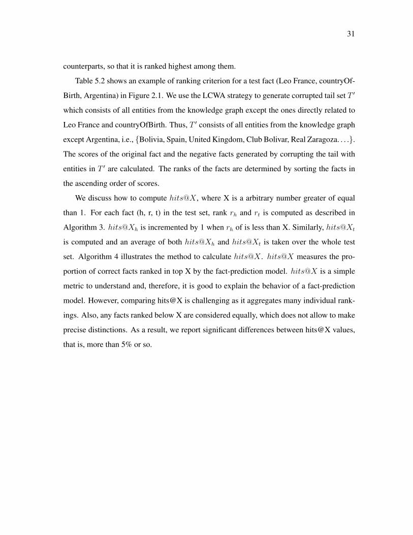
We discuss how to compute hits@X , where X is a arbitrary number greater of equal

than 1. For each fact (h, r, t) in the test set, rank rh and rt is computed as described in

Algorithm 3. hits@Xh is incremented by 1 when rh of is less than X. Similarly, hits@Xt

is computed and an average of both hits@Xh and hits@Xt is taken over the whole test

set. Algorithm 4 illustrates the method to calculate hits@X . hits@X measures the pro-

portion of correct facts ranked in top X by the fact-prediction model. hits@X is a simple

metric to understand and, therefore, it is good to explain the behavior of a fact-prediction

model. However, comparing hits@X is challenging as it aggregates many individual rank-

ings. Also, any facts ranked below X are considered equally, which does not allow to make

precise distinctions. As a result, we report significant differences between hits@X values,

that is, more than 5% or so.

32

Table 5.2: Example of ranking Criterion

Fact Score Rank(Leo France, countryOfBirth, Argentina) 64 1

(Leo France, countryOfBirth, Spain) 112 2(Leo France, countryOfBirth, Bolivia) 145 3

(Leo France, countryOfBirth, United Kingdom) 159 4(Leo France, countryOfBirth, Club Bolivar) 165 5

(Leo France, countryOfBirth, Real Zaragoza) 180 6

Algorithm 3: RankingCriterionInput: Test set GTE , corrupted head set H ′, corrupted tail set T ′, negative fact

generation strategy S, trained model M

Output: rank of (h, r, t) when head is corrupted rh, rank of (h, r, t) when tail is

corrupted rt

1 for (h, r, t) ∈ GTE do

2 Th = corrupth(S, (h, r, t)) ;

3 Tt = corruptt(S, (h, r, t)) ;

4 rh ← 1 rt ← 1 for (h′, r, t) ∈ Th do

5 if score(M, (h′, r, t)) < score(M, (h, r, t)) then

6 rh ← rh + 1

7 end

8 end

9 for (h, r, t′) ∈ Tt do

10 if score(M, (h, r, t′)) < score(M, (h, r, t)) then

11 rt ← rt + 1

12 end

13 end

14 end

33

Algorithm 4: ComputeHits@XInput: Test set GTE , arbitrary number X , corrupted head set H ′, corrupted tail set

T ′, negative fact generation strategy S, trained model M

Output: hits@X

1 for (h, r, t) ∈ GTE do

2 rh, rt ← RankingCriterion(GTE, X,H′, T ′, S,M);

3 hits@Xh ← 0 ;

4 hits@Xt ← 0 ;

5 if rh ≤ X then

6 hits@Xh ← hits@Xh + 1

7 end

8 if rt ≤ X then

9 hits@Xt ← hits@Xt + 1

10 end

11 end

12 hits@X = 12|T |(hits@Xh + hits@Xt)

5.5 Results

We evaluated TransE (E), TransD (D), and TransH (H) using naive, LCWA, TLCWA, and

NLCWA and reported hits@10, i.e., the percentage of facts ranked 10th or above in GTE

for the datasets listed in Table 5.1. Since each negative fact generation strategy is expected

to produce a different number of negative facts with different levels of semantic plausibility,

the model is trained using one strategy at a time and tested using all strategies. A robust

model can discard the maximum percentage of negative facts produced by each testing

strategy.

34

Table 5.3: Training with naıve

Naıve LCWA TLCWA NLCWAD E H D E H D E H D E H

FB13 1 .78 .76 .26 .18 .18 .27 .29 .29 .27 .29 .29FB15K237 1 .99 .99 .19 .14 .13 .27 .25 .25 .23 .20 .19NELL-995 .95 .85 .85 .43 .27 .26 .54 .28 .29 .53 .28 .28WN18RR .84 .80 .79 .01 .02 .02 .03 .03 .03 .01 .02 .02YAGO3-10 .95 .70 .69 .12 .05 .05 .14 .13 .13 .13 .13 .13

Table 5.4: Training with LCWA

Naıve LCWA TLCWA NLCWAD E H D E H D E H D E H

FB13 .72 .51 .56 .39 .20 .23 .39 .30 .33 .39 .30 .33FB15K237 .98 .96 .96 .45 .35 .36 .48 .37 .39 .47 .36 .37NELL-995 .84 .54 .57 .55 .27 .27 .62 .29 .29 .61 .28 .29WN18RR .68 .60 .60 .45 .37 .37 .46 .38 .39 .45 .38 .38YAGO3-10 .83 .51 .49 .38 .08 .08 .40 .17 .18 .39 .17 .18

Training with naıve: When the model is trained using naıve, it achieves high accuracy

when tested with naıve itself (Table 5.3). The model’s accuracy drops significantly on

testing with LCWA, TLCWA, and NLCWA. In the case of WN18RR, the accuracy is close

to zero. We believe such a vast difference in accuracy is because the model can recognize

more of nonsensical facts produced by naıve rather than challenging, semantically plausible

facts produced by other strategies. The variation in the accuracy by testing strategy is

evident across all translation-based models.

Training with LCWA: Contrasting to the model trained with naıve (Table 5.3), the

model trained with LCWA (Table 5.4) has lower accuracy when tested with naıve. For

all datasets, the difference is more than 10-30% except for FB15K237. The accuracy in-

creases significantly when tested with other strategies. However, the accuracy appears to

be similar when tested with either LCWA, TLCWA, or NLCWA except for NELL.

35

Table 5.5: Training with TLCWA

Naıve LCWA TLCWA NLCWAD E H D E H D E H D E H

FB13 .14 .01 .01 .12 0 0 .43 .15 .15 .41 .15 .15FB15K237 .46 .22 .22 .17 .06 .08 .54 .42 .43 .31 .14 .16NELL-995 .53 .24 .25 .42 .16 .16 .81 .59 .59 .74 .40 .40WN18RR .59 .42 .43 .45 .34 .34 .51 .39 .40 .49 .37 .37YAGO3-10 .36 .15 .16 .19 .06 .07 .48 .26 .29 .40 .19 .20

Table 5.6: Training with NLCWA

Naıve LCWA TLCWA NLCWAD E H D E H D E H D E H

FB13 .22 .06 .04 .10 .01 0 .43 .16 .16 .42 .16 .16FB15K237 .85 .79 .71 .37 .26 .26 .51 .41 .40 .49 .37 .38NELL-995 .68 .45 .46 .56 .33 .33 .79 .57 .60 .78 .56 .56WN18RR .59 .48 .48 .45 .36 .36 .49 .39 .39 .48 .38 .38YAGO3-10 .52 .26 .23 .26 .07 .06 .49 .24 .25 .46 .20 .20

Training with TLCWA: Compared to the models trained with naıve (Table 5.3) and

LCWA (Table 5.4), the model trained with TLCWA (Table 5.5) achieves lower accuracy

when tested with naıve and LCWA. Since TLCWA takes into account more restrictive neg-

ative facts for training, the model fails to recognize most of the negative facts generated

by naıve and LCWA. The accuracy increases consistently on testing with TLCWA and

NLCWA for all datasets except when FB13 is tested with TransE and TransH.

Training with NLCWA: The model trained with NLCWA (Table 5.6) performs slightly

better on testing with naıve and LCWA as compared to the model trained with TLCWA

(Table 5.5). However, we do not observe major differences in the accuracy on testing

with TLCWA and NLCWA. NLCWA considers additional entities for corruption based on

the compatibility of relations in the neighborhood. Seldom compatible relations are not

found in the neighborhood and the model simply relies on entities generated with TLCWA.

Hence, the accuracy of the model trained with TLCWA and NLCWA does not lie far from

each other.

36

Table 5.7: Training with naıve + NLCWA

Naıve LCWA TLCWA NLCWAD E H D E H D E H D E H

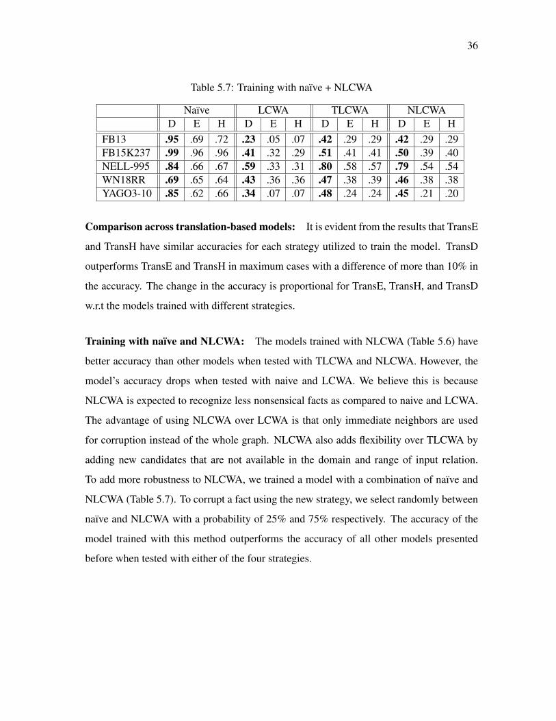
FB13 .95 .69 .72 .23 .05 .07 .42 .29 .29 .42 .29 .29FB15K237 .99 .96 .96 .41 .32 .29 .51 .41 .41 .50 .39 .40NELL-995 .84 .66 .67 .59 .33 .31 .80 .58 .57 .79 .54 .54WN18RR .69 .65 .64 .43 .36 .36 .47 .38 .39 .46 .38 .38YAGO3-10 .85 .62 .66 .34 .07 .07 .48 .24 .24 .45 .21 .20

Comparison across translation-based models: It is evident from the results that TransE

and TransH have similar accuracies for each strategy utilized to train the model. TransD

outperforms TransE and TransH in maximum cases with a difference of more than 10% in

the accuracy. The change in the accuracy is proportional for TransE, TransH, and TransD

w.r.t the models trained with different strategies.

Training with naıve and NLCWA: The models trained with NLCWA (Table 5.6) have

better accuracy than other models when tested with TLCWA and NLCWA. However, the

model’s accuracy drops when tested with naive and LCWA. We believe this is because

NLCWA is expected to recognize less nonsensical facts as compared to naive and LCWA.

The advantage of using NLCWA over LCWA is that only immediate neighbors are used

for corruption instead of the whole graph. NLCWA also adds flexibility over TLCWA by

adding new candidates that are not available in the domain and range of input relation.

To add more robustness to NLCWA, we trained a model with a combination of naıve and

NLCWA (Table 5.7). To corrupt a fact using the new strategy, we select randomly between

naıve and NLCWA with a probability of 25% and 75% respectively. The accuracy of the

model trained with this method outperforms the accuracy of all other models presented

before when tested with either of the four strategies.

37

Chapter 6

Conclusions

6.1 Conclusion

Negative facts produced with naıve and LCWA strategies are expected to be nonsensical

rather than semantically plausible. NLCWA and TLCWA are expected to produce fewer

nonsensical and more semantically plausible negative facts. We observed that the accuracy

of the model varies w.r.t the different strategies used. When models are trained with naıve

and LCWA strategies, they recognize better nonsensical facts than semantically plausible

facts. Models trained with NLCWA and TLCWA are good at recognizing semantically

plausible facts but struggle to recognize nonsensical facts. A model trained with a combi-

nation of NLCWA and naıve performs similar to LCWA, i.e., NLCWA+ naıve ≈ LCWA.

This suggests that models can be trained using subgraphs based on neighboring facts in-

stead of whole graphs.

6.2 Future Work

The local-closed world assumption uses the entire knowledge graph to generate negative

facts which are expensive. Therefore, utilizing neighborhood-based strategies we can train

individual models based on subgraphs. Different negative fact generation strategies should

be reevaluated based on individual models.

Currently, the datasets are randomly split that alters the topology of the knowledge

graph and the training split does not resemble the original graph. Thus, new ways of split-

ting can be incorporated in further analysis. Current metrics are calculated based on only

38

the ranks of facts that do not consider the number of negative facts generated per positive

fact. Designing a new metric that weighs the number of negative equivalents could be

useful for further study.

In NLCWA, we consider the immediate neighbors of relations for generating possible

candidates for corruption. Although this gives us additional candidates as compared to

that in TLCWA, it does not give us the complete set of entities for corruption. Instead

of depending on the immediate neighbors, we can extend the search to k-neighbors and

reassess the model accuracy.

39

Bibliography

[1] Farahnaz Akrami, Mohammed Saeef, Qingheng Zhang, Wei Hu, and Chengkai Li.Realistic re-evaluation of knowledge graph completion methods: An experimentalstudy, 03 2020.

[2] Soren Auer, Christian Bizer, Georgi Kobilarov, Jens Lehmann, Richard Cyganiak, andZachary Ives. Dbpedia: A nucleus for a web of open data. In Proceedings of the 6thInternational The Semantic Web and 2nd Asian Conference on Asian Semantic WebConference, ISWC’07/ASWC’07, page 722–735, Berlin, Heidelberg, 2007. Springer-Verlag.

[3] Laure Berti-Equille. Ml-based knowledge graph curation: Current solutions and chal-lenges. In Companion Proceedings of The 2019 World Wide Web Conference, WWW’19, page 938–939, New York, NY, USA, 2019. Association for Computing Machin-ery.

[4] Kurt Bollacker, Colin Evans, Praveen Paritosh, Tim Sturge, and Jamie Taylor. Free-base: a collaboratively created graph database for structuring human knowledge. InProceedings of the 2008 ACM SIGMOD international conference on Management ofdata, pages 1247–1250, 2008.

[5] Antoine Bordes and Evgeniy Gabrilovich. Constructing and mining web-scale knowl-edge graphs: Kdd 2014 tutorial. In Proceedings of the 20th ACM SIGKDD Interna-tional Conference on Knowledge Discovery and Data Mining, KDD ’14, page 1967,New York, NY, USA, 2014. Association for Computing Machinery.

[6] Antoine Bordes, Nicolas Usunier, Alberto Garcia-Duran, Jason Weston, and OksanaYakhnenko. Translating embeddings for modeling multi-relational data. In Proceed-ings of the 26th International Conference on Neural Information Processing Systems -Volume 2, NIPS’13, page 2787–2795, Red Hook, NY, USA, 2013. Curran AssociatesInc.

40

[7] David Carral, Cristina Feier, Bernardo Cuenca Grau, Pascal Hitzler, and Ian Horrocks.Pushing the boundaries of tractable ontology reasoning. In Peter Mika, Tania Tu-dorache, Abraham Bernstein, Chris Welty, Craig Knoblock, Denny Vrandecic, PaulGroth, Natasha Noy, Krzysztof Janowicz, and Carole Goble, editors, The SemanticWeb – ISWC 2014, pages 148–163, Cham, 2014. Springer International Publishing.

[8] Tim Dettmers, Pasquale Minervini, Pontus Stenetorp, and Sebastian Riedel. Con-volutional 2d knowledge graph embeddings. In Thirty-Second AAAI Conference onArtificial Intelligence, 2018.

[9] Xin Luna Dong, Evgeniy Gabrilovich, Geremy Heitz, Wilko Horn, Ni Lao, KevinMurphy, Thomas Strohmann, Shaohua Sun, and Wei Zhang. Knowledge vault: Aweb-scale approach to probabilistic knowledge fusion. In The 20th ACM SIGKDDInternational Conference on Knowledge Discovery and Data Mining, KDD ’14, NewYork, NY, USA - August 24 - 27, 2014, pages 601–610, 2014. Evgeniy GabrilovichWilko Horn Ni Lao Kevin Murphy Thomas Strohmann Shaohua Sun Wei ZhangGeremy Heitz.

[10] Lucas Drumond, Steffen Rendle, and Lars Schmidt-Thieme. Predicting rdf triplesin incomplete knowledge bases with tensor factorization. In Proceedings of the 27thAnnual ACM Symposium on Applied Computing, SAC ’12, page 326–331, New York,NY, USA, 2012. Association for Computing Machinery.

[11] Christiane Fellbaum. Wordnet. The encyclopedia of applied linguistics, 2012.

[12] Luis Antonio Galarraga, Christina Teflioudi, Katja Hose, and Fabian Suchanek.Amie: association rule mining under incomplete evidence in ontological knowledgebases. In Proceedings of the 22nd international conference on World Wide Web, pages413–422, 2013.

[13] Shu Guo, Quan Wang, Bin Wang, Lihong Wang, and Li Guo. Semantically smoothknowledge graph embedding. In Proceedings of the 53rd Annual Meeting of theAssociation for Computational Linguistics and the 7th International Joint Conferenceon Natural Language Processing (Volume 1: Long Papers), pages 84–94, 2015.

[14] Xu Han, Shulin Cao, Xin Lv, Yankai Lin, Zhiyuan Liu, Maosong Sun, and JuanziLi. OpenKE: An open toolkit for knowledge embedding. In Proceedings of the2018 Conference on Empirical Methods in Natural Language Processing: System

41

Demonstrations, pages 139–144, Brussels, Belgium, November 2018. Associationfor Computational Linguistics.

[15] Aidan Hogan, Eva Blomqvist, Michael Cochez, Claudia d’Amato, Gerard de Melo,Claudio Gutierrez, Jose Labra Gayo, Sabrina Kirrane, Sebastian Neumaier, AxelPolleres, Roberto Navigli, Axel-Cyrille Ngonga Ngomo, Sabbir Rashid, AnisaRula, Lukas Schmelzeisen, Juan Sequeda, Steffen Staab, and Antoine Zimmermann.Knowledge graphs. 03 2020.

[16] Viet-Phi Huynh and Paolo Papotti. A benchmark for fact checking algorithms builton knowledge bases. In Proceedings of the 28th ACM International Conference onInformation and Knowledge Management, CIKM ’19, page 689–698, New York, NY,USA, 2019. Association for Computing Machinery.

[17] Guoliang Ji, Shizhu He, Liheng Xu, Kang Liu, and Jun Zhao. Knowledge graph em-bedding via dynamic mapping matrix. In Proceedings of the 53rd annual meetingof the association for computational linguistics and the 7th international joint con-ference on natural language processing (volume 1: Long papers), pages 687–696,2015.

[18] Bhushan Kotnis and Vivi Nastase. Analysis of the impact of negative sampling onlink prediction in knowledge graphs. arXiv preprint arXiv:1708.06816, 2017.

[19] Denis Krompaß, Stephan Baier, and Volker Tresp. Type-constrained representationlearning in knowledge graphs. In International semantic web conference, pages 640–655. Springer, 2015.

[20] Yankai Lin, Zhiyuan Liu, Huanbo Luan, Maosong Sun, Siwei Rao, and Song Liu.Modeling relation paths for representation learning of knowledge bases. arXivpreprint arXiv:1506.00379, 2015.

[21] Yankai Lin, Zhiyuan Liu, Maosong Sun, Yang Liu, and Xuan Zhu. Learning entityand relation embeddings for knowledge graph completion. In Twenty-ninth AAAIconference on artificial intelligence, 2015.

[22] Farzaneh Mahdisoltani, Joanna Biega, and Fabian M Suchanek. Yago3: A knowledgebase from multilingual wikipedias. 2013.

42

[23] T. Mitchell, W. Cohen, E. Hruschka, P. Talukdar, J. Betteridge, A. Carlson, B. Dalvi,M. Gardner, B. Kisiel, J. Krishnamurthy, N. Lao, K. Mazaitis, T. Mohamed, N. Nakas-hole, E. Platanios, A. Ritter, M. Samadi, B. Settles, R. Wang, D. Wijaya, A. Gupta,X. Chen, A. Saparov, M. Greaves, and J. Welling. Never-ending learning. In Pro-ceedings of the Twenty-Ninth AAAI Conference on Artificial Intelligence (AAAI-15),2015.

[24] Heiko Paulheim. Knowledge graph refinement: A survey of approaches and evalua-tion methods. Semantic Web, 8:489–508, 12 2016.

[25] Heiko Paulheim and Christian Bizer. Type inference on noisy rdf data. In Interna-tional semantic web conference, pages 510–525. Springer, 2013.

[26] Ian S. Robinson, Jim Webber, and Emil Eifrem. Graph databases. 2013.

[27] Sebastian Ruder. An overview of gradient descent optimization algorithms. arXivpreprint arXiv:1609.04747, 2016.

[28] Richard Socher, Danqi Chen, Christopher D Manning, and Andrew Ng. Reasoningwith neural tensor networks for knowledge base completion. In Advances in neuralinformation processing systems, pages 926–934, 2013.

[29] Kristina Toutanova and Danqi Chen. Observed versus latent features for knowledgebase and text inference. In Proceedings of the 3rd Workshop on Continuous VectorSpace Models and their Compositionality, pages 57–66, 2015.

[30] Kristina Toutanova, Xi Victoria Lin, Wen-tau Yih, Hoifung Poon, and Chris Quirk.Compositional learning of embeddings for relation paths in knowledge base and text.In Proceedings of the 54th Annual Meeting of the Association for Computational Lin-guistics (Volume 1: Long Papers), pages 1434–1444, 2016.

[31] Denny Vrandecic and Markus Krotzsch. Wikidata: A free collaborative knowledge-base. Commun. ACM, 57(10):78–85, September 2014.

[32] Quan Wang, Zhendong Mao, Bin Wang, and Li Guo. Knowledge graph embedding:A survey of approaches and applications. IEEE Transactions on Knowledge and DataEngineering, PP:1–1, 09 2017.

43

[33] Zhen Wang, Jianwen Zhang, Jianlin Feng, and Zheng Chen. Knowledge graph andtext jointly embedding. In Proceedings of the 2014 conference on empirical methodsin natural language processing (EMNLP), pages 1591–1601, 2014.

[34] Zhen Wang, Jianwen Zhang, Jianlin Feng, and Zheng Chen. Knowledge graph em-bedding by translating on hyperplanes. In Twenty-Eighth AAAI conference on artifi-cial intelligence, 2014.

[35] Robert West, Evgeniy Gabrilovich, Kevin Murphy, Shaohua Sun, Rahul Gupta, andDekang Lin. Knowledge base completion via search-based question answering. InProceedings of the 23rd International Conference on World Wide Web, WWW ’14,page 515–526, New York, NY, USA, 2014. Association for Computing Machinery.

[36] Robert West, Evgeniy Gabrilovich, Kevin Murphy, Shaohua Sun, Rahul Gupta, andDekang Lin. Knowledge base completion via search-based question answering. InProceedings of the 23rd International Conference on World Wide Web, WWW ’14,page 515–526, New York, NY, USA, 2014. Association for Computing Machinery.

[37] Ruobing Xie, Zhiyuan Liu, and Maosong Sun. Representation learning of knowledgegraphs with hierarchical types. In IJCAI, pages 2965–2971, 2016.

[38] Huaping Zhong, Jianwen Zhang, Zhen Wang, Hai Wan, and Zheng Chen. Aligningknowledge and text embeddings by entity descriptions. In Proceedings of the 2015Conference on Empirical Methods in Natural Language Processing, pages 267–272,2015.

44

Appendix A

Code Listing

The datasets, code for translation-based models, and negative fact generation strategies are

available here: https://github.com/crrivero/ImpactNegativeTriples.

A.1 Python code to generate negative facts

The code to generate negative facts during training and testing is listed below. The

negativeFactGeneration class creates the corrupted head and tail sets H’ and T’ for either

of the negative fact generation strategies mentioned in Chapter 3. The constructor of the

class creates the domain, range, dictionary to store the head associated with every relation

and tail, and dictionary to store the tail associated with every relation and head. The

corruptHeadTail function accepts the corruptionMode and compatible relations as input

for each fact and produces two sets of corrupted head H’ and tail T’: headCorruptedDict

and tailCorruptedDict.

1 c l a s s n e g a t i v e F a c t G e n e r a t i o n ( ) :23 def i n i t ( s e l f , d a t a s e t ) :4 s e l f . e n t i t y S e t = s e t ( )5 s e l f . h e a d S e t = s e t ( )6 s e l f . t a i l S e t = s e t ( )7 s e l f . domain = {}8 s e l f . range = {}9 s e l f . h e a d D i c t = {}

10 s e l f . t a i l D i c t = {}11 s e l f . h e a d C o r r u p t e d D i c t = {}12 s e l f . t a i l C o r r u p t e d D i c t = {}

45

13 s e l f . newDomain = {}14 s e l f . newRange = {}15 s e l f . d a t a s e t = d a t a s e t1617 f o r ( h , r , t ) in s e l f . d a t a s e t :18 s e l f . e n t i t y S e t . add ( h )19 s e l f . e n t i t y S e t . add ( t )20 s e l f . h e a d S e t . add ( h )21 s e l f . t a i l S e t . add ( t )22 i f r not in s e l f . domain :23 s e l f . domain [ r ] = s e t ( )24 s e l f . domain . add ( h )25 i f r not in s e l f . range :26 s e l f . range [ r ] = s e t ( )27 s e l f . range . add ( t )28 i f r not in s e l f . h e a d D i c t :29 s e l f . h e a d D i c t [ r ] = {}30 e l s e :31 i f t not in s e l f . h e a d D i c t [ r ] :32 s e l f . h e a d D i c t [ r ] [ t ] = s e t ( )33 s e l f . h e a d D i c t [ r ] [ t ] . add ( h )34 i f r not in s e l f . t a i l D i c t :35 s e l f . t a i l D i c t [ r ] = {}36 e l s e :37 i f h not in s e l f . t a i l D i c t [ r ] :38 s e l f . t a i l D i c t [ r ] [ h ] = s e t ( )39 s e l f . t a i l D i c t [ r ] [ h ] . add ( t )4041 def c o r r u p t H e a d T a i l ( s e l f , co r rup t ionMode , c o m p a t i b l e R e l a t i o n s ) :42 f o r ( h , r , t ) in s e l f . d a t a s e t :43 i f c o r r u p t i o n M o d e == ” Naive ” :44 s e l f . h e a d C o r r u p t e d D i c t [ r ] [ t ] = \45 s e l f . e n t i t y S e t − s e l f . h e a d S e t46 s e l f . t a i l C o r r u p t e d D i c t [ r ] [ h ] = \47 s e l f . e n t i t y S e t − s e l f . t a i l S e t48 e l i f c o r r u p t i o n M o d e == ”LCWA” :49 s e l f . h e a d C o r r u p t e d D i c t [ r ] [ t ] = \50 s e l f . e n t i t y S e t − s e l f . h e a d D i c t [ r ] [ t ]51 s e l f . t a i l C o r r u p t e d D i c t [ r ] [ h ] = \52 s e l f . e n t i t y S e t − s e l f . t a i l D i c t [ r ] [ h ]53 e l i f c o r r u p t i o n M o d e == ”TLCWA” :54 s e l f . h e a d C o r r u p t e d D i c t [ r ] [ t ] = \55 s e l f . domain [ r ] − s e l f . h e a d D i c t [ r ] [ t ]56 s e l f . t a i l C o r r u p t e d D i c t [ r ] [ h ] = \57 s e l f . range [ r ] − s e l f . t a i l D i c t [ r ] [ h ]58 e l i f c o r r u p t i o n M o d e == ”NLCWA” or c o r r u p t i o n M o d e ==”GNLCWA” :

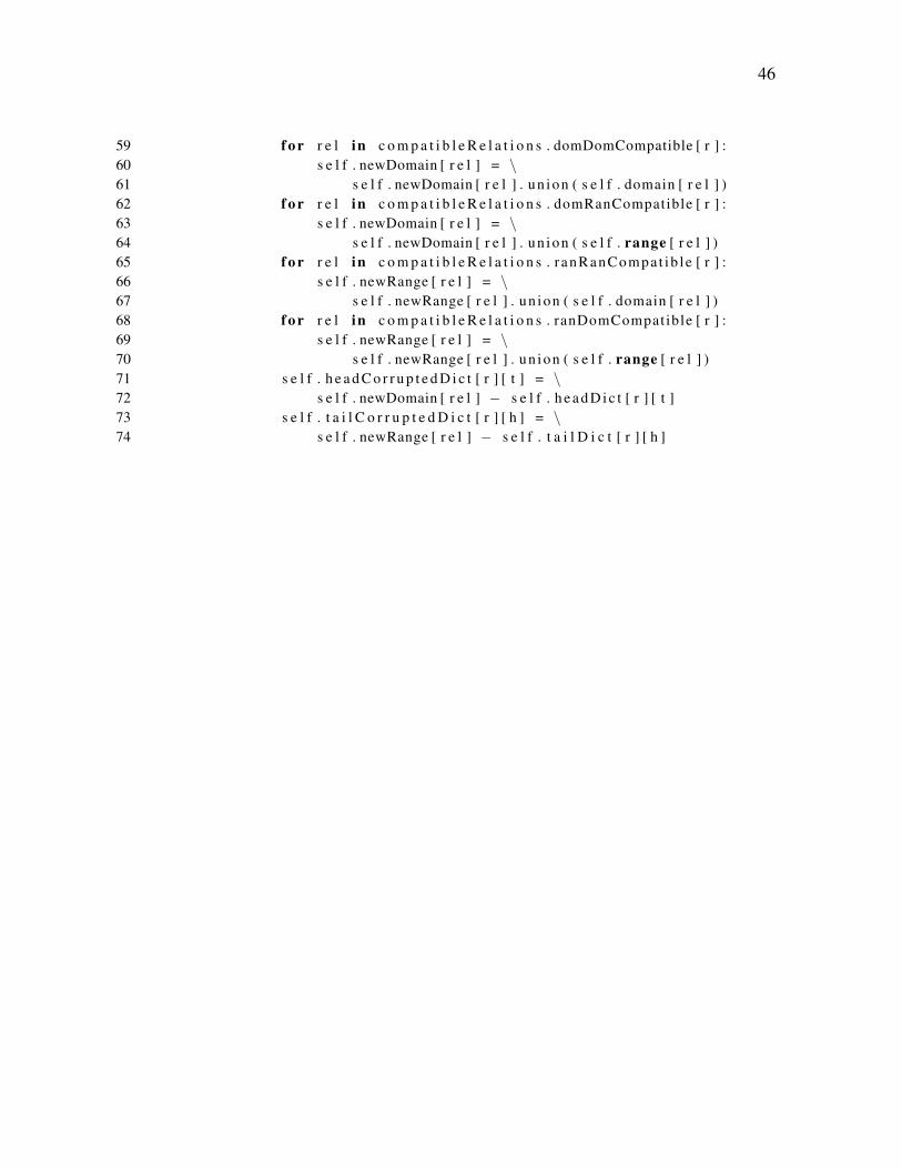
46

59 f o r r e l in c o m p a t i b l e R e l a t i o n s . domDomCompatible [ r ] :60 s e l f . newDomain [ r e l ] = \61 s e l f . newDomain [ r e l ] . un ion ( s e l f . domain [ r e l ] )62 f o r r e l in c o m p a t i b l e R e l a t i o n s . domRanCompatible [ r ] :63 s e l f . newDomain [ r e l ] = \64 s e l f . newDomain [ r e l ] . un ion ( s e l f . range [ r e l ] )65 f o r r e l in c o m p a t i b l e R e l a t i o n s . r anRanCompa t ib l e [ r ] :66 s e l f . newRange [ r e l ] = \67 s e l f . newRange [ r e l ] . un ion ( s e l f . domain [ r e l ] )68 f o r r e l in c o m p a t i b l e R e l a t i o n s . ranDomCompatible [ r ] :69 s e l f . newRange [ r e l ] = \70 s e l f . newRange [ r e l ] . un ion ( s e l f . range [ r e l ] )71 s e l f . h e a d C o r r u p t e d D i c t [ r ] [ t ] = \72 s e l f . newDomain [ r e l ] − s e l f . h e a d D i c t [ r ] [ t ]73 s e l f . t a i l C o r r u p t e d D i c t [ r ] [ h ] = \74 s e l f . newRange [ r e l ] − s e l f . t a i l D i c t [ r ] [ h ]