Analyzing the analysts: When do

recommendations add value?

Narasimhan Jegadeesh University of Illinois at Urbana-Champaign

Joonghyuk Kim

Case Western Reserve University

Susan D. Krische University of Illinois at Urbana-Champaign

Charles M. C. Lee* Cornell University

Current Draft: November 6, 2001

Comments welcomed

* This paper subsumes two earlier manuscripts titled “Stock Characteristics and Analyst Stock Recommendations” and “The Information Content of Analyst Stock Recommendations.” We have benefited from the comments of Bill Beaver, Louis Chan, Tom Dyckman, Paul Irvine, Josef Lakonishok, Michael Weisbach, and Kent Womack, as well as workshop participants at University of California – Berkeley, Case Western Reserve University, Cornell University, Dartmouth College, Emory University, Georgetown University, University of Illinois at Urbana-Champaign, Rice University, the University of Rochester, University of Southern California, University of Colorado, and the Prudential Securities Quantitative Research Conference. We would also like to thank Zacks Investment Research for providing the analyst recommendation data and I/B/E/S for providing the analyst earnings forecasts. First Call Corporation als o provided us with recommendations data used in one of our earlier manuscripts.

2

Analyzing the analysts: When do

recommendations add value?

Abstract

We show that financial analysts from sell-side firms generally recommend

“glamour” (i.e., positive momentum, high growth, high volume, and

relatively expensive) stocks. Naïve adherence to these recommendations

can be costly, because the level of the consensus recommendation adds

value only among stocks with positive quantitative characteristics (i.e.,

high value and positive momentum stocks). Among stocks with negative

quantitative characteristics, higher consensus recommendations are

associated with worse subsequent returns. In contrast, the quarterly

change in the consensus recommendation is a robust return predictor that

appears to contain information orthogonal to a large range of other

predictive variables.

1. Introduction

Financial researchers and practitioners have long been interested in understanding how

the activities of financial analysts affect capital market efficiency. Currently in the

United States, over 3,000 analysts work for more than 350 sell-side investment firms.1

These analysts produce corporate earnings forecasts, write reports on individual

companies, provide industry and sector analyses, and issue stock recommendations.

Most prior studies have concluded that the information they produce promotes market

efficiency by helping investors to value companies’ assets more accurately.2

Analysts gather and process a variety of information about different stocks, form their

beliefs about the intrinsic stock values relative to their current market prices, and finally

rate the investment potential of each stock. As Elton, Gruber, and Grossman (1986, page

699) observe, these recommendations represent “one of the few cases in evaluating

information content where the forecaster is recommending a clear and unequivocal

course of action rather than producing an estimate of a number, the interpretation of

which is up to the user.” In short, these recommendations offer a unique opportunity to

study analyst judgment and preferences across large samples of stocks.

In this study, we investigate analyst preferences across stocks, and evaluate the sources of

the investment value provided by analyst stock recommendations and recommendation

changes. We expect this research to be of interest to both financial academics and

practitioners. From an academic perspective, the study contributes to a better

understanding of how analysts evaluate stocks, and their role in the price formation

process. From the perspective of investors, this research enhances our understanding of

the usefulness (and limitations) of analyst recommendations in investment decisions.

1 See www.bulldogresearch.com. These statistics do not include “Associates” and other junior analysts that

provide research support. 2 For reviews of this literature, see Schipper (1991) and Brown (2000).

2

Finally, from the perspective of sell-side analysts, our study provides a decision aid for

making better recommendations (in terms of improved returns prediction).3

The first part of the study presents a descriptive profile of the firms preferred by analysts.

This research is designed to provide insights on analysts’ consistency with various stock

characteristics in developing their stock recommendations.4 The firm characteristics we

consider are measures that have a demonstrated ability to forecast cross-sectional returns

in prior studies. In the context of this study, these variables serve three purposes. First,

they allow us to examine the extent to which the predictive power of stock

recommendations is due to analysts' tendency to recommend stocks that appear attractive

based on other well-known pricing anomalies.5 Second, they help us to understand how

analyst recommendations are related to “momentum” and “contrarian” investment

strategies. Finally, these predictive variables allow us to evaluate the extent to which

analysts incorporate concurrently available information in their recommendations.

Our results show that analysts generally prefer “glamour” stocks to “value” stocks.

Stocks that receive higher recommendations (as well as more favorable recommendation

revisions) tend to have positive momentum (both price and earnings) and high trading

volume (as measured by their turnover ratio). They exhibit greater past sales growth, and

are expected to grow their earnings faster in the future. These stocks also tend to have

higher valuation multiples, more positive accounting accruals, and they invest a greater

proportion of their total assets in capital expenditures.

3 This statement assumes that analysts are interested in improving the predictive power of their

recommendations. As we discuss later, due to incentive issues, optimal returns prediction may not be the primary goal of analysts.

4 Our approach is similar in spirit to Brunswick’s lens model analysis, common in experimental research, in which a decision-maker assesses various information cues to predict a criterion event (e.g., see Libby (1981) for further discussions). Examples of this research related to analysts’ stock recommendations include Pankoff and Virgil (1970) and Mear and Firth (1987, 1990); see also Ebert and Kruse (1978).

5 Prior studies controlled for firm characteristics, such as book-to-market, firm size, and price momentum (e.g., see Womack (1996) and Barber et al. (2001a)). We investigate a much larger set of variables including accounting accruals, capital expenditures, past trading volume, past growth, and forecasted future growth.

3

However, we show that this preference for growth stocks is not always in line with the

interests of the investing public. Specifically, we find that analyst recommendations fail

to incorporate the predictive power of most so-called “contrarian” indicators. In the case

of seven out of eight contrarian signals, the correlation with analysts’ stock

recommendations is directionally opposite to the variable’s correlation with future

returns.

The analysts’ penchant for growth firms is consistent with the economic incentives

imposed by their operating environment. Most sell-side analysts work for brokerage

houses whose primary businesses are investment banking, and sales and trading. Growth

firms and firms with higher trading activity make more attractive clients to the brokerage

firms. These incentives may cause analysts to, knowingly or otherwise, tilt their attention

and stock recommendations in favor of growth and high volume stocks.

We find that, in spite of their general disagreement with the other predictive variables,

stocks favorably recommended by the analysts outperform stocks unfavorably

recommend by them. This result is consistent with the evidence documented by Barber,

Lehavy, McNichols, and Trueman (2001a). However, we find that the level of analyst

recommendation derives its predictive power largely from a tilt towards high momentum

stocks. After controlling for the return predictability of the other signals, we find that the

marginal predictive ability of the level of analyst recommendation is not significant.

We find that a key reason for the poor performance of the level variable is due to

analysts’ failure to quickly downgrade stocks rejected by the other signals. For stocks

where the other signals predict low future returns, favorably recommended stocks

significantly underperform unfavorably recommended stocks. For this subset of stocks,

perhaps favorable analyst recommendations temporarily support prices and delay the

eventual incorporation of information in the predictive signals into stock prices.

However, within the subset of stocks where other signals predict high future returns,

stocks favorably recommended by analysts outperform stocks unfavorably recommended

by them.

4

We also find that upgraded stocks outperform downgraded stocks, consistent with the

findings in Womack (1996). The predictive power of recommendation changes

(revisions) is more robust than the predictive power of the level of analyst

recommendations. Specifically, we find that recommendation changes add value to

characteristic-based investment strategies that include 12 other predictive variables.

In sum, our results show that analyst recommendations exhibit a style bias in favor of

growth over value. That is, they prefer positive momentum stocks with higher growth

trajectories that look expensive on most valuation metrics. In the parlance of the

behavioral finance literature (e.g., Hong and Stein (1999)), sell-side analysts are better

characterized as “trend chasers” than “news watchers.” We believe analysts’ penchant

for growth-style stocks is consistent with their job incentives. Nevertheless, this behavior

reduces the effectiveness of their recommendations as a predictor of subsequent returns.

Partly due to this bias, the level of analyst recommendation provides little incremental

investment value over the other investment signals. However, in spite of a similar bias,

recent changes in recommendations provide incremental value. This finding suggests

that either: (1) sell-side analysts bring information to market through their

recommendation changes that is largely orthogonal to the other signals, or, (2) they create

their own price momentum by virtue of their stature as “opinion makers.” In our

concluding section, we discuss implications of these findings for academic research on

behavioral finance and financial accounting.

The remainder of the paper is organized as follows. Section 2 describes the motivation

for this study and develops our hypotheses in the context of prior studies. Section 3

presents our research methodology and sample selection procedures. Sections 4 and 5

evaluate the incremental investment value of recommendations and changes in

recommendations. Section 6 summarizes our findings and discusses some of their

implications.

5

2. Analyst recommendations and stock characteristics

This paper provides a link between the literature on analyst recommendations and studies

on the predictability of cross-sectional returns. The first part of the study provides a

descriptive profile of firms that receive stronger recommendations, as well as firms that

analysts tend to upgrade (downgrade). This part of our analysis is similar in spirit to

recent studies by Finger and Landsman (1999) and Stickel (1999). However, given our

interest in the role of analyst recommendations in investment decisions, our focus is on

explanatory variables that have a demonstrated ability to predict future returns. Our

main interest lies in the correlation of these variables with contemporaneous

recommendations.

The twelve predictive variables we examine are nominated by prior studies in accounting

and finance. We evaluate the predictive ability of analyst recommendations in light of

these variables. Womack (1996) and Elton et al. (1986) show that firms that receive buy

(sell) recommendations tend to earn higher (lower) abnormal returns in the subsequent

one to six months.6 Barber et al. (2001a) extend the investigation to consensus

recommendations, documenting the potential to earn higher returns by buying the most

highly recommended stocks and short selling the least favorably recommended stocks.

We investigate the extent to which this price drift phenomenon is due to analysts'

tendency to issue recommendations consistent with a wide set of investment strategies.

We also compare and contrast the predictive ability of consensus recommendation levels

and changes. To our knowledge this is the first study to conduct such a comparison.

2.1 Predictive Variables

We consider twelve variables that have demonstrated their ability to predict cross-

sectional returns. The Appendix contains detailed information on how each variable is

computed. These variables are also summarized below.

6 Specifically, Womack (1996) examine new added-to-buy and added-to-sell recommendations, while Elton

et al. (1986) examine excess returns in the first calendar month after brokerage recommendation changes.

6

2.1.1 Momentum and Trading Volume – The first five explanatory variables are based on

a stock’s recent trading activities and earnings news. Jegadeesh and Titman (1993) show

that firms with higher (lower) price momentum earn higher (lower) returns over the next

12 months. We capture the price momentum effect with two variables: RETP (RET2P)

is the cumulative market-adjusted return for each stock in months –6 through –1 (−12

through –7) preceding the month of the recommendation.

Prior studies also show that recent earnings momentum predicts cross-sectional returns

(e.g., Chan, Jegadeesh, Lakonishok (1996), Bernard and Thomas (1989)). Specifically,

firms with upward revisions in earnings and positive earnings surprises earn higher

subsequent returns. We capture the earnings momentum effect with two variables:

FREV is the analyst earnings forecast revision computed as a rolling sum of over the six

months prior to the month of the recommendation, scaled by price. SUE is the

unexpected earnings for the most recent quarter, scaled by its time-series standard

deviation over the eight preceding quarters.

TURN is a measure of the average daily volume turnover for the stock in the six months

preceding the month of the recommendation. Lee and Swaminathan (2000) show that

high (low) volume stocks exhibit glamour (value) characteristics, and earn lower (higher)

returns in subsequent months.7 They argue that TURN is a contrarian signal, and that

high (low) turnover stocks are over-valued (under-valued) by investors.

If analysts based their recommendations on the predictive attributes of price (and

earnings) momentum, as well as trading volume, we would expect past winners and

lower-volume stocks (past losers and higher-volume stocks) to receive the most favorable

(least favorable) recommendations.

7 As noted in Lee and Swaminathan (2000), trading volume for NASDAQ stocks is inflated by the

presence of inter-dealer trades, and is not comparable to the volume reported for stocks traded on the NYSE or AMEX. To adjust for this effect, we compute a percentile rank score by exchange.

7

2.1.2 Valuation Multiples – We also consider two valuation multiples: EP (the earnings-

to-price ratio) and BP (the book-to-price ratio). Both variables are widely used in value-

based investment strategies. Starting with Basu (1977), a number of academic studies

show that high EP firms subsequently outperform low EP firms. Similarly, Fama and

French (1992), among others, show that high BP firms subsequently earn higher returns

than low BP firms. Academic opinions differ on whether these higher returns represent

contrarian profits or a fair reward for risk.8 In either case, if analysts pay attention to the

predictive attribute of these multiples, we would expect high EP (and high BP) firms to

receive more favorable recommendations.

2.1.3 Growth Indicators – We include two growth indicators: LTG (the mean analyst

forecast of expect long-term growth in earnings) and SGI (the rate of growth in sales

over the past year). Lakonishok, Shleifer and Vishny (1994) show that firms with high

past growth in sales earn lower subsequent returns. They argue that high growth firms

are glamour stocks that are over-valued by the market.9 In the same spirit, La Porta

(1996) shows that firms with high forecasted earnings growth (high LTG firms) also earn

lower subsequent returns. If analysts rely on these large sample results, low SGI (and

low LTG) firms should receive more favorable recommendations.

2.1.4 Firm Size – Fama and French (1992), among others, show that small firms have

generally earned higher returns than large firms. While opinions differ on the robustness

of the result and the interpretation of this variable, we include a control for firm size.

Specifically, we compute SIZE as the natural log of a firm’s market capitalization at the

end of its most recent fiscal quarter.

2.1.5 Fundamental Indicators – Finally, we include two fundamental indicators from the

accounting literature: TA (total accruals divided by total assets) and CAPEX (capital

8 See, for example, the discussions in Fama and French (1992) and Lakonishok et al. (1994) for two

alternative interpretations of the evidence. 9 Lakonishok et al. (1994) use a variable that measures the change in sales over the past five years. Our

variable is the one-year growth rate in sales, which Beneish (1999) shows is useful in detecting firms that manipulate their earnings.

8

expenditures divided by total assets). TA provides a measure of the quality of earnings,

and could signal earnings manipulation. For example, if firms excessively capitalize

overheads into inventories, or if they fail to write off inventories in a timely manner, then

the inventory component of accruals will rise. Such accounting gimmicks lead to

positive accruals. Sloan (1996) finds that firms with low accruals (more negative TA)

earn higher future returns than firms with high accruals. He argues that the accrual-

component of earnings is less persistent, and that the market does not take this effect into

account in a timely fashion.

However, Chan, Chan, Jegadeesh and Lakonishok (2001) point out that firms with large

sales growth will experience large increases in accounts receivables and inventory,

mainly to support the increased levels of sales. In fact, Chan et al. (2001) find that the

decile of firms with the largest accruals experience sales growth of 22% per year over the

prior three year period compared to 7% per year sales growth for the decile of low

accrual firms. They also find large earnings growth for high accrual firms. Therefore,

accruals may be symptoms of managerial manipulation in some instances, but high

accruals are also associated with strong past operating performance.

Beneish, Lee, and Tarpley (2001) show that growth firms with high CAPEX also tend to

earn lower returns. Such firms are over represented in the population of extreme losers

(so called “torpedoed” stocks). They argue that high CAPEX firms are growth firms that

tend to over-extend themselves. Again, if analysts pay attention to these results, lower

TA (and lower CAPEX) firms should receive more favorable recommendations.

To summarize, all twelve variables we use have demonstrated an ability to predict cross-

sectional returns in prior studies. While not an exhaustive list, these variables do capture

much of what is known about large-sample tendencies in expected returns. To the extent

that analysts are either explicitly or intuitively aware of these tendencies, these variables

may be reflected in their stock recommendations. If so, we would expect the variables to

be correlated with analyst recommendations in the same way they are correlated with

future returns.

9

3. Sample Selection and Research Design

3.1 Sample Selection

Our initial sample consists of all the stocks in the Zacks Investment Research

recommendations database for the period 1985 through 1998.10 Zacks collects the

recommendations from contributors and assigns standardized numerical ratings (1=strong

buy, 3=hold, 5=strong sell). To allow for a more intuitive interpretation of the

quantitative results, we code the recommendations so that more favorable

recommendations receive a higher score (e.g., 5=strong buy, 3=hold, 1=strong sell).

For each firm, we calculate the consensus recommendation level (CONS) and the

consensus recommendation change (CHGCONS) at the end of each calendar quarter.

The consensus recommendation level is the mean of all outstanding recommendations for

a given firm, issued a minimum of two days and a maximum of 12 months prior to the

calendar quarter end. We only use the most recent recommendation for a given analyst.

The consensus recommendation change is the increase (or decrease) in the consensus

recommendation level, from the end of the prior calendar quarter to the end of the current

calendar quarter.

For each observation, we require that the firm’s market price information be available in

the CRSP database, that its earnings forecasts be available in the I/B/E/S database, and

that its accounting information be available on the merged quarterly COMPUSTAT

database. These data constraints ensure the availability of basic financial information for

each firm in our sample. A firm-quarter observation is included in our final sample only

if all twelve of the investment signals (previously discussed, and described in detail in the

Appendix) are available for that quarter.

10 Zacks obtains the recommendations from written reports provided by brokerage firms and uses the date

of the recommendation as the date of the brokerage firm report. The academic database from Zacks does not include recommendations from several large brokerage houses, most notably Merrill Lynch, Goldman Sachs, and Donaldson, Lufkin, and Jenrette.

10

Figure 1 illustrates the data collection periods for each of our empirical measures. For a

consensus recommendation level observed at the end of quarter t, we use market-related

data (past returns, and trading volume) and analyst-related data that are collected up to 12

months prior to the end of quarter t. For accounting-related data, we identify the most

recent quarter for which an earnings announcement was made at least two months prior to

the end of quarter t, and calculate the accounting data based on the rolling-sum of this

and the three prior quarters. Subsequent return accumulation begins with the first trading

day of quarter t+1.

These procedures ensure that: (1) the latest annual financial statements are available to

the analysts at the time of their recommendation, (2) this financial information is

reasonably fresh for all sample firms, and (3) future returns reflect potentially tradable

strategies.

3.2 Data Description

Our data collection procedure yielded an average of 971.4 firm-observations per quarter

over the 56 quarters. Table 1 provides descriptive statistics on the number of observations

by year (Panel A), by exchange (Panel B), and by NYSE size decile (Panel C). Panel A

shows that the average number of firm-observations has increased over time from 1985

through 1998. Panel B shows that approximately 56% (44%) of our observations consists

of NASDAQ (NYSE/AMEX) firms. Finally, Panel C shows these observations are

evenly distributed across the NYSE size deciles, but that size varies by exchange.

Additional analyses (not reported) show that these firms span a large number of different

industries, with no single industry representing more than 8.1% of the total sample.

Table 2 reports information on the distribution of the consensus recommendation levels

and changes. Recall that, to allow for a more intuitive interpretation of the quantitative

results, we code the recommendations so that more favorable recommendations receive a

higher score (e.g., 5=strong buy, 1=strong sell). For both the consensus recommendation

levels and changes, we also group the firm-observations into quintiles, calculated

separately for each quarter. The quintiles are labeled 0.00, 0.25, and so on to 1.00, where

11

0.00 contains the quintile of firms with the least favorable ratings and 1.00 contains the

quintile of firms with the most favorable ratings. In the case of recommendation changes,

all “no change” observations are included in the middle change quintile.

Panel A of table 2 reports descriptive statistics for five consensus recommendation level

quintiles, calculated separately for each of the 56 quarters (1.00=strong buy, 0.50=hold,

0.00=strong sell). It is clear from these results that analysts rarely issue sell or strong-sell

recommendations. The mean consensus recommendation level in the bottom consensus

level quintile is only a hold (2.76).11

Panel B reports the change in analyst recommendations, defined as the current quarter

recommendation level minus the prior quarter recommendation level. Quintiles are

calculated separately for each of the 55 quarters (1.00=strong increase, 0.50=hold,

0.00=strong decrease), but with all “no change” observations included in the middle

quintile. In our sample, analysts were slightly more likely to downgrade a firm than

upgrade it (mean change = −0.01).

Panel C provides evidence on the negative correlation between the level of the prior

consensus recommendation, and changes in the consensus. A firm that received a

relatively high (low) prior recommendation is much more likely to be down (up) graded.

For example, 32.2% of the firms in the top quintile in terms of the prior consensus appear

in the bottom quintile in terms of changes in the consensus recommendation. Conversely,

29.0% of the firms in the bottom quintile of prior consensus recommendations appear in

the top changes quintile. In subsequent tests, we control for this strong negative

correlation.

11 Commercial services that report analyst recommendations (e.g., Zacks, First Call and IBES), generally

assign a lower score to more favorable recommendations (i.e., 1=strong buy, 5=strong sell). To reconcile our score with the score reported by these services, subtract our score from 6. For example, the mean consensus recommendation level in our sample is equivalent to a rating of 2.33 (6.00 - 3.67) in Zacks. The mean consensus in the bottom levels quintile is equivalent to a Zacks rating of 3.24 (6.00 – 2.76).

12

4. Empirical Results

4.1 Analyst Recommendations and Future Returns

Table 3 provides evidence on the predictive ability of analyst stock recommendations.

For this table, we only report results for a six-month holding period. Panel A reports the

Spearman rank correlation between the two recommendation measures and market-

adjusted returns for the six months following the month of recommendation. These

correlations are computed each quarter. Table values represent the mean and median

correlations over 56 quarters for levels and 55 quarters for changes. The Mean results are

based on two-sided T-tests with Hansen-Hodrick autocorrelation adjusted statistics; the

Median results are based on two-sided Wilcoxon signed-rank tests. The table reports the

correlation for the continuous variables, as well as the categorical variables based on

quintile assignments as defined in Table 2.

Table 3 confirms prior studies in that both CONS and CHGCONS are correlated with

future returns. Specifically, firms that receive more favorable recommendations (buys or

upgrades) earn higher subsequent returns than firms that receive less favorable

recommendations (sells/holds or downgrades). Recall that our recommendation variables

are based on month-end information. Therefore, these results likely under-estimate the

predictive power of analyst recommendations, as much of the associated price adjustment

takes place in the first 2-3 weeks after the news release.12

The next two panels report the mean and median market-adjusted return in quintile

portfolios sorted each quarter by CONS, the analyst recommendation level (Panel B), and

by CHGCONS, the change in analyst recommendation (Panel C). Table values represent

the mean market-adjusted returns for each quintile portfolio. For CONS, the mean

difference between top and bottom quintile is 2.3% over the next six months. For the

12 Our results are similar in magnitude to Womack (1996), who examined individual recommendations

(specifically, he examines new buy or new sell recommendations). Compared to his study, we probably understate total returns because our holding period does not begin until the beginning of the next calendar month. Barber et al. (2001a) and Elton et al. (1986) test somewhat different implicit strategies, making direct comparisons more difficult.

13

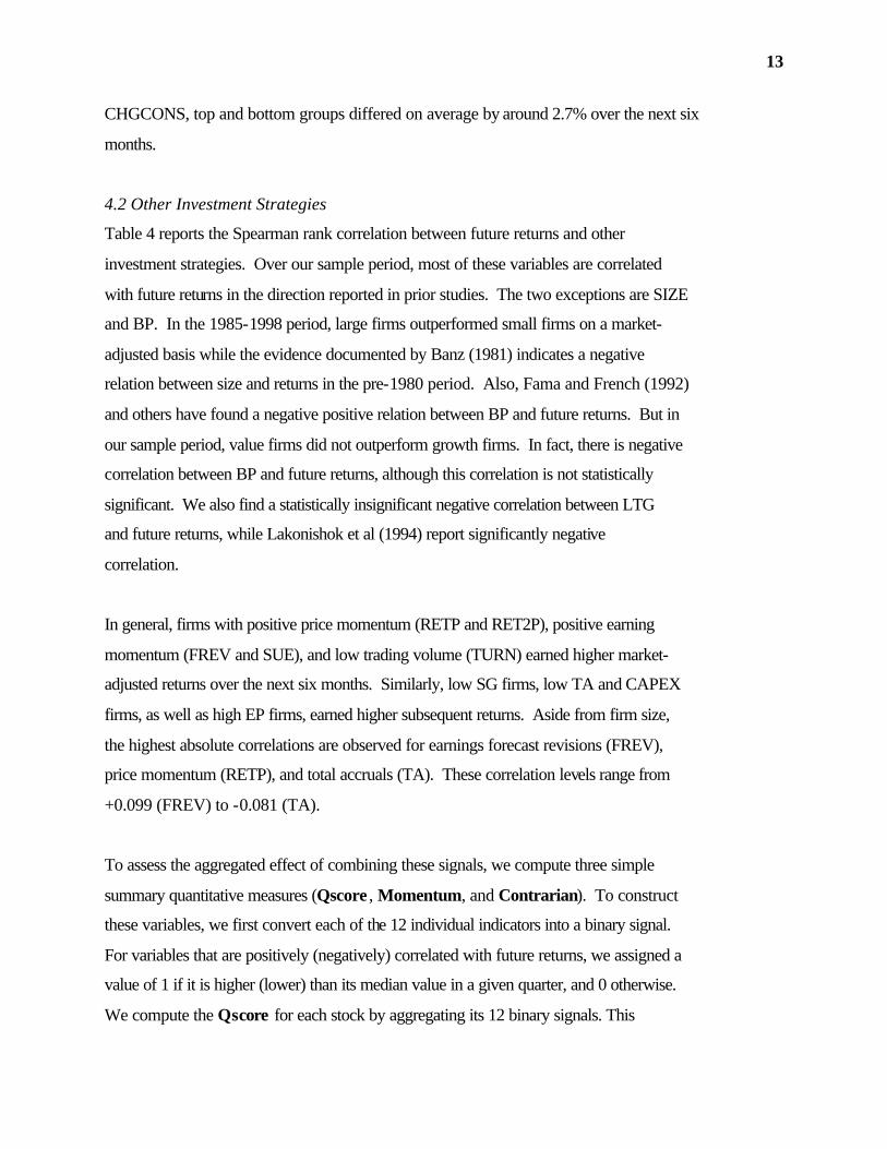
CHGCONS, top and bottom groups differed on average by around 2.7% over the next six

months.

4.2 Other Investment Strategies

Table 4 reports the Spearman rank correlation between future returns and other

investment strategies. Over our sample period, most of these variables are correlated

with future returns in the direction reported in prior studies. The two exceptions are SIZE

and BP. In the 1985-1998 period, large firms outperformed small firms on a market-

adjusted basis while the evidence documented by Banz (1981) indicates a negative

relation between size and returns in the pre-1980 period. Also, Fama and French (1992)

and others have found a negative positive relation between BP and future returns. But in

our sample period, value firms did not outperform growth firms. In fact, there is negative

correlation between BP and future returns, although this correlation is not statistically

significant. We also find a statistically insignificant negative correlation between LTG

and future returns, while Lakonishok et al (1994) report significantly negative

correlation.

In general, firms with positive price momentum (RETP and RET2P), positive earning

momentum (FREV and SUE), and low trading volume (TURN) earned higher market-

adjusted returns over the next six months. Similarly, low SG firms, low TA and CAPEX

firms, as well as high EP firms, earned higher subsequent returns. Aside from firm size,

the highest absolute correlations are observed for earnings forecast revisions (FREV),

price momentum (RETP), and total accruals (TA). These correlation levels range from

+0.099 (FREV) to -0.081 (TA).

To assess the aggregated effect of combining these signals, we compute three simple

summary quantitative measures (Qscore , Momentum, and Contrarian). To construct

these variables, we first convert each of the 12 individual indicators into a binary signal.

For variables that are positively (negatively) correlated with future returns, we assigned a

value of 1 if it is higher (lower) than its median value in a given quarter, and 0 otherwise.

We compute the Qscore for each stock by aggregating its 12 binary signals. This

14

aggregation process gives us a measure that captures how these signals work together in

quantitative investment strategies. We chose this simple measure rather than conduct a

search for a more efficient return predictor because it is not our goal to create an optimal

measure to predict future returns.

We also separately compute a Momentum score by aggregating the binary scores across

the momentum signals RETP, RET2P, FREV, and SUE. We aggregate the remaining

scores across the remaining signals to obtain the Contrarian score. We label these

signals as contrarian because typically when these signals are associated with high future

growth in earnings or sales, they tend to be associated with low future returns.

Under the column heading “% Positive”, Table 4 reports the percent of total observations

that received a value of “1” for each investment signal. Under the column heading

“Correlation”, we report the Spearman rank correlation of these binary variables with

future returns. As expected, correlation levels are slightly lower when we move from the

continuous variable to this binary coding. However, the binary versions of most

variables still exhibit statistically significant correlations with future returns. The “Mean

net portfolio return” is the mean difference in returns between the portfolio of top firms

(with binary variable equal to 1) and the portfolio of bottom firms (with binary variable

equal to 0). The final column in this table indicates the percentage of the 56 quarters in

which the net portfolio return was above 0%.

Table 5 examines the correlation between three summary quantitative variables and

future returns, defined as the market-adjusted return over the next six months. The three

summary variables are: Momentum (the sum of the four momentum signals: RETP,

RET2P, FREV, and SUE), Contrarian (the sum of the remaining eight signals), and

QScore (the sum of all twelve binary signals). Panel A reports the Spearman rank

correlation between each summary measure and future returns. We report results for both

a continuous measure and a quintile measure of the summary variable (see Table 2).

Panel B reports future returns grouped by QScore quintiles, Panel C reports future returns

15

grouped by Momentum quintiles, and Panel D reports future returns for firms grouped by

Contrarian quintiles.

Panel A shows that all three summary variables are positively correlated with future

returns. QScore has the highest mean Spearman rank correlation (0.125), but both

Momentum and Contrarian are positively correlated with future returns (approximately

0.09). Panel B shows that the mean (median) difference between top and bottom QScore

quintile returns is 5.71% (7.70%). The mean (median) difference for the Momentum

ranking (Panel C) is approximately equal, at 5.73% (6.20%). The mean (median) return

difference between the extreme Contrarian quintiles (Panel D) is 3.64% (7.86%). For all

three variables, the mean and median returns decline monotonically as we move down the

five quintiles. Clearly, these summary variables are correlated with future returns during

our sample period.

4.3 Analyst Recommendations and Investment Strategies

Thus far, we have established the predictive ability of the investment signals in our

sample. We have also documented the predictive ability of the analyst stock

recommendations. In this section, we examine the relation between analyst

recommendations and various investment signals.

Table 6 reports the mean and median value of each of the 12 investment signals by

consensus recommendation quintile. Under the heading “Normative Direction,” we show

the direction of correlation between each variable and future market-adjusted return as

indicated by prior research. Under the heading “Actual Direction” we report the direction

of correlation between that variable and the analysts’ consensus recommendation in our

sample. We also report the Spearman rank correlation between each variable and the

consensus recommendation. In addition, we provide T-tests of the null that the mean

value is the same for the top and bottom consensus recommendation quintiles.

Table 6 shows that analysts’ consensus recommendations correspond well with the

Momentum indicators. Specifically, analysts exhibit a strong preference for positive

16

momentum stocks. In fact, the Spearman rank correlation between analyst

recommendations and the four momentum variables range from 26.9% to 34.6%. In

particular, analysts seem to recommend most strongly firms with recent upward earnings

forecast revisions (FREV) and positive earnings surprises (SUE).

But perhaps the most striking result in Table 6 is the consistency with which analyst

stock recommendations contradict the expected normative usage of the Contrarian

variables. In seven out of eight cases, the actual direction of the analysts’ preference is

opposite to the normative direction for predicting future stock returns. Analysts prefer

stocks with high recent turnover (TURN) over stocks with low turnover. They also

prefer large SIZE, low BP, high SG, high LTG, high TA, and high CAPEX stocks. In

fact, the only contrarian variable that analysts seem to get “right” is EP – they prefer

stocks that have higher earnings-to-price ratios to stocks that have lower earnings-to-

price ratios.13

Table 7 provides additional evidence in a multivariate setting. This table reports results

when each recommendation variable is regressed on the 12 explanatory variables. Panel

A (B) reports results when the dependent variable is the level of (change in) the

consensus recommendation. With few exceptions, Table 7 confirms the univariate results

reported in Table 6. Panel A shows that, with the exception of BP, the level of the

consensus recommendation continues to run counter to the Contrarian variables. Panel B

shows that changes in the consensus recommendation are also consistent with the

Momentum variables, and counter to the Contrarian variables. In other words, analysts

tend to revise their recommendations upwards (downwards) for positive (negative)

momentum stocks. However, they also tend to revise their recommendation upwards for

high TURN, high LTG, high SG, and high CAPEX firms.

13 Bradshaw (2000) shows that analyst recommendations are correlated with a firm’s PEG ratio. Our

results contain both components of the PEG ratio (the P/E ratio and the forecasted earnings growth). These findings are consistent, because even in our sample, analysts exhibit a strong preference for high LTG firms (Spearman rank correlation of 27.2%).

17

An interesting exception is the total accruals variable (TA). While the level of the

consensus recommendation is positively correlated with TA, the change in the consensus

appears is negatively correlated with TA. These results suggest that analysts revise their

recommendations in a manner consistent with the information content of accruals. In

other words, while mean recommendation levels favor firms with income increasing

accruals, when analysts revise their recommendations, firms with income decreasing

(income increasing) accruals tend to receive upward (downward) revisions. The

implication is that analysts do not initially pay sufficient attention to the quality of

earnings as revealed by TA, but they adjust in the right direction over time.

The general picture that emerges from the analysis is that analysts favorably recommend

stocks with strong past operating performance and stocks that are expected to deliver

healthy improvements in operating performance in the future. High SUE for the most

favorably recommended stocks indicates that these stocks had strong operating

performance in the past. Large FREV indicate that analysts have favorably revised their

expectations about the future operating performance of these stocks. In the same spirit,

high recent returns capture favorable revisions in market expectations about future

operating performance.

The contrarian signals that analysts prefer also suggest that they pick stocks with strong

operating performance. For example, analysts prefer low BP firms and high TA firms.

Low BP firms generally have higher returns-on-equity (ROE), and are expected to enjoy

faster growth in profitability in the future. Similarly, high TA firms on average have

faster sales growth than low TA firms (see Chan et al. 2000). Historically, however, the

contrarian characteristics that analysts prefer (with the exception of EP) are associated

with lower future returns. These findings indicate that when there is a conflict between

indicators of strong operating performance, and the large sample empirical relation

between the signals and future returns, analysts tend to make their recommendations on

the basis of strong past operating performance.

18

In sum, these findings show that the momentum signals preferred by analysts will help in

the performance of their recommendations, but their contrarian signal preferences will

likely hurt their performance. In the next section, we evaluate the predictive power of

analyst recommendations in conjunction with the other twelve signals.

5. Incremental Value of Analyst Recommendations

In this section, we evaluate the incremental value of analyst recommendations, and

changes in these recommendations, when these signals are used in conjunction with other

predictive signals.

5.1 Multivariate Analysis

We first examine the relation between future returns and QCON and QCHGCON. As a

starting point, we define future returns as the market–adjusted return in the six months

after the month of the recommendation (RETF). Table 8 reports the regression

coefficients averaged across the quarters in the sample. Because RETF overlaps across

quarters, we use autocorrelation-consistent standard errors to compute the t-statistic.14

Model A1 in Panel A is a univariate regression, with RETF as the dependent variable and

QCON as the independent variables each quarter. The results show that the coefficient

on QCON is positive and statistically significant in this regression, indicating that when

used alone, it helps predict future returns.

To assess whether QCON incrementally predicts returns when used in conjunction with

the 12 characteristic-based signals, we consider three different regression specifications.

In the first multivariate regression, we use the QCON and Qscore as independent

variables (Model A2). These results show that QCON loses its statistical significant once

QScore is introduced.

14 Since the return overlap is over one quarter, we allow for the first-order serial correlation to be different

from zero while computing the autocorrelation-consistent standard errors.

19

Next, we consider a regression model where we use QCON and the 12 signals as separate

independent variables (Model A3). This specification pits each of these signals against

QCON individually rather than at an aggregated level. With the exception of BP and

SIZE, the other investment signals are all correlated with future returns in the expected

direction. However, only RETP, FREV, TA, and CAPEX, are individually significant.

QCON is not significant in this regression.

Collectively, the evidence from Model A2 and Model A3 suggests that while QCONS is

weakly correlated with returns, its contribution is minor when considered in conjunction

with the other signals. However, these models may be somewhat handicapped against

QCON because they allow the slope coefficients for the independent variables to take the

``right'' sign in predicting returns. In most instances, the binary contrarian signals are

negatively correlated with QCON but they are positively correlated with future returns.

As a final test, we fit a regression where the independent variable that we use in addition

to QCON is and its fitted value (Qfitcon) from the regression in Table 7, Panel A (Model

A4). Interestingly, QCON is not statistically significant in this regression, but Qfitcon is

significant. This evidence indicates that the investment value of QCON is largely due to

its tilt towards firm characteristics that are related to future returns.

Table 8, Panel B reports the results for regressions with QCHGCONS. Model B1 shows

that QCHGCONS is able to predict future returns. The estimated coefficient (2.25%) can

be interpreted as the hedge return between the extreme CHGCONS quintiles over the

next six months. Notice that the estimated coefficient and the t-statistic on QCHGCONS

both decrease as we introduce QScore and the other control variables (Models B2 to B3).

In the last regression specification (Model B4), we include the fitted value (Qfitchgcon)

for QCHGCON from the regression in Table 7, as well as QCHGCON, in the regression.

Model B3 shows that this variable remains statistically significant in the presence of all

12 other investment signals. Model B4 shows that it is significant even with the inclusion

of Qfitchgcon. This evidence shows that QCHGCONS is incrementally useful in

20

predicting returns. In fact, in Models B3 and B4, it is the explanatory variable associated

with the highest t-statistic.15

5.2 Two-way analysis

Although analyst recommendations do not add value to the general population of stocks

when used in conjunction with other characteristics, it is possible that they may add

incremental value for subsets of stocks. In this subsection, we examine the performance

of analyst recommendations and recommendation changes within quintiles of stocks

ranked partitioned based on the summary scores.

Table 9 reports results of a two-way analysis, in which firms are sorted by their

quantitative summary score (QScore), as well as by their analyst recommendation (CONS

or CHGCONS). Panel A of this table reports results for the level of the consensus

recommendation (CONS). Panel B reports results for individual recommendations

(CHGCONS). Panel C reports results for a combined strategy involving both level and

change quintiles. For this panel, Worst (Best) firms are firms that are in both the lowest

(highest) CONS and the lowest (highest) CHGCONS quintile. All other firms are

assigned to a middle category.

Panel A reports six month market-adjusted returns of firms sorted by CONS and QScore.

Looking along the bottom row of each panel, it is clear that the QScore variable has

significant predictive power for returns after controlling for the analyst recommendation.

High QScore firms earn significantly higher subsequent returns in all analyst

recommendation categories. QScore performs particularly well among firms with the

highest analyst recommendation. In that category, the return difference between top and

bottom QScore firms is 9.10% over the next six months.

15 The holding period for the strategies tested in our paper includes the year 1999, but not 2000. Barber et

al. (2001b) report that during the calendar year 2000, stocks least favorably recommended by analysts earned higher subsequent returns than stocks that are highly recommended. However, their tests only examine the level of the consensus variable, which has marginal predictive power even during our sample period.

21

The results along the right column of each panel show that analyst recommendations

(CONS) have some limited predictive power after controlling for QScore, but this power

is conditional on the QScore quintile. Specifically, CONS is only useful among high

QScore firms. In the highest QScore quintile, top CONS quintile firms earn 3.24% more

than bottom CONS quintile firms over the next six months. However, for firms with a

low QScore, the return to a CONS strategy is negative. This result suggests that among

low QScore stocks, firms more highly recommended by the analysts actually do worse in

the future than firms with low recommendations.

Another result that emerges from this table is that when analyst recommendations and the

QScore signal disagree, the QScore signal tends to dominate. The cells along the off

diagonal of each panel (toward the lower-left and upper-right corners) report mean

returns when the QScore and the analyst recommendation signals are in disagreement. In

Panel A, firms in the lower-left corner (High QScore firms with low recommendations)

earn higher average returns than firms in the upper-right corner (Low QScore firms with

high recommendations). The return difference of 5.86% (labeled “DISAGREE”) is

statistically significant at the 1% level. Evidently, when the two signals conflict, the

QScore results in more reliable returns predictions.

Finally, when the two signals agree, we find the highest predictive power for returns. In

the lower-right corner of each panel, labeled “AGREE”, we report the return differential

when analyst recommendations are combined with the QScore indicator. These cells

show the mean return differential between firms with the best recommendations and

highest QScores (Best-and-High), and firms with the worst recommendations and lowest

QScores (Worst-and-Low). In all three panels, the Best-and-High group earns higher

returns than the Worst-and-Low group. The returns differential ranges from 7.03% to

9.35% over the next six months, which is greater than returns earned by considering

either signal alone.

Figure 2 depicts the cumulative excess return from various hedge strategies involving

both analyst recommendations and the QScore. The results for the six-month holding

22

period are the same as those reported in Table 9, but Figure 2 extends Table 9 by

reporting the cumulative excess return over different holding periods (1, 3, 6, 9 and 12

months). Each graph reports the returns to three strategies. The High-Low strategy

involves taking an equal-weighted long position in the top QScore quintile firms and

short selling an equal-weighted position in the bottom QScore quintile firms. The Best-

Worst strategy involves buying the highest recommended firms and selling the lowest

recommended firms. The Combined strategy buys the Best-and-High group and sells the

Worst-and-Low group.

As indicated by Panel A, the level of the consensus recommendation (CONS) has limited

ability to predict returns. The hedge return to the ANALYST variable in this graph never

exceeds 2.2% (at the six month horizon). When used in combination with QScore, this

variable adds a modest 1.5% to the mean QScore strategy’s return over six months.

Panels B shows that portfolios formed on the basis of the change in the consensus

recommendation (CHGCONS) performs somewhat better. When CHGCONS is used

alone, the Increase-Decrease hedge strategy based on top and bottom quintiles generates

2.7% over six months, and 3.6% over 12 months. When combined with QScore, this

variable adds approximately 2% to the QScore strategy returns over six months.

Panel C reports the results when both CONS and CHGCONS are used. As indicated in

Table 9, this double filter results in fewer positions being taken (an average of 13.3 buys

and 24.3 shorts per month). At the same time, the cumulative excess return based on the

analyst variable alone increases to 5.3% over six months. When used it combination with

QScore, this combined strategy adds almost 4% to the excess return of the QScore

strategy over six months. These results suggest that the two analyst recommendation

measures are not redundant for returns prediction.

Table 10 provides a more comprehensive analysis of the cumulative excess returns to

analyst recommendation strategies over various holding periods. To construct this table,

firms are grouped each quarter into quintiles by their quantitative score (QScore,

Momentum, and Contrarian), as well as consensus recommendation (either CONS or

23

CHGCONS). Panel A reports the mean difference in market-adjusted returns between

the extreme CONS quintiles (BUY-SELL) within each quantitative measure quintile over

55 quarters. Panel B repeats the analysis for CHGCONS. We report the cumulative

excess return for 1, 3, 6, 9, and 12 month holding periods for each strategy. Positive

(negative) table values indicate that the strategy generated mean favorable (unfavorable)

excess returns over the holding period.

Several facts emerge from this table. First, as we have seen earlier, CHGCONS is a

better predictor of returns than CONS. Panel B shows that CHGCONS strategies

generate positive returns over all holding periods and in all quintiles formed on QScore,

Momentum, and Contrarian. In contrast, a strategy based on CONS is far less consistent.

Panel A shows that, controlling for QScore, a CONS based strategy is almost as likely to

yield negative excess returns as positive excess returns.

Second, analysts are more likely to add value to contrarian investing strategies. In both

panels, the analysts seem to better compliment the Contrarian strategy than the

Momentum strategy. This result perhaps is not surprising, because we have seen earlier

that some of the analyst’s predictive power derives from their tendency to select positive

momentum stocks.

Third, Table 10 shows that the main reason the CONS strategy is less reliable is because

it generates positive excess returns only in high QScore quintiles. In low QScore

quintiles, the excess returns to a CONS based strategy are reliably negative. In other

words, when selecting among firms with unfavorable quantitative signals, it is better to

invest against analyst recommendations than to invest according to these

recommendations. This result is quite striking and is stronger as the holding period

lengthens. Moreover, it is observed within both Momentum quintile partitions and

Contrarian quintile partitions.

Figure 3 provides a graphic illustration of the different roles played by CONS and

CHGCONS in return prediction. These figures show the difference in mean returns

24

between the extreme recommendation quintiles across the quintiles of each quantitative

investment signal. Across the bottom of each figure is the holding period of the strategy.

The darker bars correspond to low quintiles by each summary quantitative score (QScore,

Momentum, and Contrarian), the lighter bars correspond to high quintiles.

Panel A shows that the CONS strategy yields positive returns for high QScore quintiles

(lighter bars), but the same strategy yields negative returns for low QScore quintiles

(darker bars). Apparently the level of the consensus recommendation (CONS) is a

favorable indicator of future returns only when a firm is in the higher QScore (or higher

Momentum, higher Contrarian) quintiles. In other words, analysts seem to be able to

further identify the superior firms among a set of firms that already have favorable

fundamental or operating characteristics. However, when a firm is in the lower

Momentum or Contrarian quintiles, analyst recommendations operate in the wrong

direction, and it would be unwise to follow their stock picks. In fact, when a firm has

unfavorable fundamental or operating characteristics, it is better to trade against the

consensus analyst recommendations.

Panel B shows that the same pattern does not appear for CHGCONS. In all sub-

portfolios and over all holding periods, this strategy results in positive excess returns. In

other words, the analysts revise their recommendations in a manner that is consistent with

subsequent returns. However, the level of their consensus recommendation is only a

useful return predictor when it is confirming the quantitative investment signals.

In sum, Tables 8 through 10 show that the predictive power of analyst stock

recommendations derives largely from their correlation with the other explanatory

variables. The usefulness of the consensus level measure (QCON) is conditional on the

quantitative investment signal. Specifically, QCON is a useful predictor of returns only

when it serves to confirm favorable quantitative signals. The incremental usefulness for

returns prediction is most pronounced for the change of the consensus recommendation

(QCHGCON).

25

6. Conclusion

In making a stock recommendation, financial analysts explicitly express their expectation

about the relative near-term return performance of a given firm. In this study, we

examine the relation of their recommendations to other concurrently available public

information. We focus on variables that prior studies show have some predictive power

for future returns, and critically evaluate the investment value of these recommendations

in light of the other signals.

We find that analysts prefer growth stocks that appear over-valued by traditional

measures. On further analysis, we find that analyst recommendations are positively

correlated with momentum indicators but negatively correlated with contrarian indicators.

The stocks that receive more favorable recommendations typically have more positive

price momentum, higher trading volume (turnover), higher past and projected growth,

more positive accounting accruals, and more aggressive capital expenditures. In short,

analysts seem to recommend a set of stocks that are quite different from the stocks that

would have been nominated by quantitative investment strategies. In the parlance of

Hong and Stein (1999), financial analysts appear to be “trend chasers” rather than

fundamental “news watchers.”

We find that the level of the consensus analyst recommendation does not contain

incremental information for the general population of stocks when it is used in

conjunction with other predictive signals. For the subset of firms with favorable

momentum and contrarian signals, we find that firms favored by analysts tend to

outperform firms that are less favored. However, for the subset with less favorable

quantitative signals, the stocks that analysts recommended most favorably by analysts

actually underperform the stocks that they recommend less favorably. Perhaps, for this

subset of firms, favorable analyst recommendations actually help delay the eventual

convergence of price to the underlying fundamentals.

26

The explanatory power of the change in the consensus analyst recommendation is more

robust than that of the level of the recommendation. Changes in recommendations over

the prior quarter predict future returns when used separately and when used in

conjunction with other predictive signals. These findings suggest that the return-relevant

information contained in analyst recommendation changes is, to a large extent,

orthogonal to the information contained in the other variables.

One interpretation of our finding is that recommendation changes capture qualitative

aspects of a firm’s operations (e.g., managerial abilities, strategic alliances, intangible

assets, or other growth opportunities) that do not appear in the quantitative signals we

examine. Since we do not control for industry-related effects, it is possible that analyst

recommendation revisions reflect news about a firm’s competitive position in its industry.

The evidence is at least consistent with the analysts’ claim that they bring some new

information to market. Our findings show this information is better reflected through

changes in their recommendation than through its absolute level.

An alternative hypothesis is that the recommendations themselves cause the subsequent

price drift through the publicity surrounding them, and the subsequent marketing of these

stocks by the affiliated sales forces (Logue (1986)). In this scenario, analysts do not

actually bring new information to market via their research efforts. One way to test this

hypothesis is to check for return reversals over longer horizons. However, given our

limited sample period, it would be difficult to distinguish this scenario from the one in

which analysts are facilitating the price formation process. We regard this as an

interesting area for further research.

Our results suggest that financial analysts may be able to improve their stock

recommendations by paying more attention to the large sample attributes of expected

returns. We have identified a number of specific signals that analysts do not generally

incorporate into their recommendations. If their disregard for these signals is not

deliberate, our results may help analysts to improve their future recommendations.

Specifically, our results suggest that if analysts want to generate recommendations with

27

greater predictive power for returns, they should grant more favorable recommendations

to firms with lower trading volume, higher EP ratios, lower LTG and SG measures, more

negative (income decreasing) accruals, and lower capital expenditures.16

From an investment perspective, our results suggest analyst recommendations play a dual

role in the price formation process. On the one hand, analysts seem over-enamored with

growth and glamour stocks. To the extent that their opinion affects public sentiment, this

evidence is consistent with the view that they contribute to noise trading in the market.

On the other hand, these findings suggest analyst recommendations can still play a useful

role in investment strategies. When analyst recommendations conflict with a combined

investment signal (the QScore), the QScore dominates. However, within individual

QScore categories, analyst recommendations can be incrementally useful in returns

prediction. The change in the consensus recommendation, in particular, has significant

ability to forecast near-term (3 to 12 month) cross-sectional returns.

In contemplating its usage in investment strategies, readers need to consider several

factors. First, transaction costs issues are not explored in this study. Second, it is

possible that the top quintile stocks are riskier than the bottom quintile stocks along some

unknown dimension. This possibility is made less likely by our inclusion of 12 control

variables known to be associated with expected returns. Nevertheless, the possibility

cannot be ruled out. Finally, we show that in some circumstances (i.e., among firms with

poor quantitative scores), it is dangerous to follow analyst recommendations. Consistent

with the claim of some pundits (e.g., Der Hovanesian (2001)), the level of the analyst

recommendation itself can sometimes be a contrarian signal.

Our results suggest that fundamental analysts and investment houses that employ large-

sample quantitative techniques could each learn something from the other. Behavioral

16 This assumes that our results are not due to incentive issues. For example, if analysts recommend high

volume stocks because they are more likely to generate higher trading commissions, they are unlikely to modify their recommendations in light of our findings. The integration of these signals into analysts’ recommendations may also be hindered by psychological factors, such as analysts’ relative confidence in their own judgments (Nelson, Krische, and Bloomfield (2000)).

28

research shows that, in many cases, the combination of a human decision-maker and a

mechanical decision-aid produces the best performance (see, e.g., Blattberg and Hoch

(1990)). Assuming they are interested in predicting intermediate-horizon (3 to 12 month

ahead) returns, sell-side analysts should pay more attention to the results of large-sample

studies. On the other hand, quantitative investors could also benefit by augmenting their

stock selection process with the consensus recommendation of sell-side analysts.

Finally, we believe these results also have implications for studies in behavioral finance.

One of the major challenges confronting this emerging literature is the identification of

factors that drive investor (or noise trader) sentiment. Black (1986, page 531) defines

noise trading as “ trading on noise as if it were information.” Shiller (1984) argues that

investor sentiments arise when investors trade on pseudo-signals, such as the forecasts of

Wall Street gurus. Our results suggest that the preferences of sell-side analysts could

play a role in explaining a particular type of noise trading.

Specifically, we find that sell-side analysts (and those who follow their

recommendations) are over-enamored with high-volume, high-multiple, stocks. Lee and

Swaminathan (2000) characterize these stocks as “late-stage” momentum plays, and

show that they are particularly susceptible to subsequent price reversals. In the same

spirit, Hong and Stein (1999) argue that traders investing in late-stage momentum stocks

impose an externality on other traders by “piling on” in stocks that have already moved

too far from their fundamental value. This behavior leads to negative serial correlation in

returns over the long horizon, as prices eventually correct. Using analysts’ expressed

preferences, as revealed in their stock recommendations, we begin to put a face on the

stocks preferred by these noise traders.

29

References

Abarbanell, J. S., and R. Lehavy, 1999, Can stock recommendations predict earnings

management and analyst earnings forecast errors? Working paper, UNC-Chapel Hill

and UC-Berkeley, May.

Barber, Brad, Reuven Lehavy, Maureen McNichols, and Brett Trueman, 2001a, Can

investors profit from the prophets? Security analyst recommendations and stock

returns, Journal of Finance 56, 531-563.

, 2001b, Prophets and losses: Reassessing the returns to analysts’

stock recommendations, Working paper, UC-Davis, UC-Berkeley, and Stanford

University, May.

Basu, Sanjoy, 1977, Investment performance of common stocks in relation to their price

earnings ratios: A test of the efficient market hypothesis, Journal of Finance, 32, 663-

682.

Beneish, M. Daniel, 1999, The detection of earnings manipulation, Financial Analysts

Journal 55, September/October, 24-36.

Beneish, D. M., C. M. C. Lee, and R. Tarpley, 2001, Contextual fundamental analysis

through the prediction of extreme returns, Review of Accounting Studies, 6, 165-189.

Bernard, Victor L., and Jacob K. Thomas, 1989, Post-earnings-announcement drift:

Delayed price response or risk premium? , Journal of Accounting Research

(Supplement) 27, 1-36.

Black, Fischer, 1986, Presidential address: Noise, Journal of Finance 41, 529-543.

Blattberg, R. C., and J. S. Hoch, 1990, Database models and managerial intuition: 50%

model and 50% manager, Management Science, 36, 887-899.

30

Bradshaw, Mark, 2000, How do analysts use their earnings forecasts in generating stock

recommendations? University of Michigan working paper, January.

Brown, Lawrence D., ed., 2000, I/B/E/S Research Bibliography, Sixth Edition, I/B/E/S

International Incorporated.

Chan, Konan, Louis K. Chan, Narasimhan Jegadeesh, and Josef Lakonishok, 2001,

Earnings quality and stock returns, University of Illinois working paper, October.

Chan, Louis K., Narasimhan Jegadeesh, and Josef Lakonishok, 1996, Momentum

strategy, Journal of Finance 51, 1681-1713.

Collins, Daniel W. and Paul Hribar, 2000, Earnings-based and accrual-based market

anomalies: one effect or two? Journal of Accounting and Economics 29, 101-124.

Der Hovanesian, Mara, 2001, A definite ‘sell’? Gimme 100 shares, Business Week, April

2, 66-67.

Ebert, Ronald J., and Thomas E. Kruse, 1978, Bootstrapping the security analyst, Journal

of Applied Psychology, 63(1), 110-119.

Elton, J. Edwin, Martin J. Gruber, and Seth Grossman, 1986, Discrete expectational data

and portfolio performance, Journal of Finance, 41, 699-713.

Fama, E. F. and K. R. French, 1992, The cross-section of expected stock returns, Journal

of Finance 47, 427-465.

Finger, Catherine A., and Wayne R. Landsman, 1999, What do analysts’ stock

recommendations really mean? University of Illinois and U.N.C. – Chapel Hill

working paper, March.

31

Hong, Harrison, and Jeremy C. Stein, 1999, A unified theory of underreaction,

momentum trading and overreaction in asset markets, Journal of Finance 54, 2143-

2184.

Jegadeesh, N., and S. Titman, 1993, Returns to buying winners and selling losers:

Implications for stock market efficiency, Journal of Finance 48, 65-91.

La Porta, Raphael, 1996, Expectations and the cross-section of stock returns, Journal of

Finance 51, 1715-1742.

Lakonishok, Josef, Andrei Shleifer, and Robert W. Vishny, 1994, Contrarian investment,

extrapolation, and risk, Journal of Finance 49, 1541-1578.

Lee, C. M. C., and B. Swaminathan, 2000, Price momentum and trading volume, Journal

of Finance 55, 2017-2070.

Libby, R., 1981, Accounting and human information processing: Theory and application.

Englewood Cliffs, N. J.: Prentice-Hall.

Logue, Dennis E., 1986, Discussion: Discrete expectational data and portfolio

performance, Journal of Finance, 41, 713.

Mear, Ross, and Michael Firth, 1987, Assessing the accuracy of financial analyst security

return predictions, Accounting, Organizations and Society, 12(4), 331-340.

Mear, Ross, and Michael Firth, 1990, A parsimonious description of individual

differences in financial analyst judgment, Journal of Accounting, Auditing and

Finance, 5(4), 501-520.

Nelson, M. W., S. D. Krische, and R. J. Bloomfield, 2000, Psychological factors affecting

investors’ reliance on disciplined trading strategies, Cornell University working

paper, September.

32

Pankoff, Lyn D., and Robert L. Virgil, 1970, Some preliminary findings from a

laboratory experiment on the usefulness of financial accounting information to

security analysts, Journal of Accounting Research, 8(S), 1-48.

Schipper, K., 1991, Analysts’ forecasts, Accounting Horizons 5, 105-121.

Shiller, Robert J., 1984, Stock prices and social dynamics, The Brookings Papers on

Economic Activity 2, 457-510.

Sloan, R. G., 1996, Do stock prices fully reflect information in accruals and cash flows

about future earnings? The Accounting Review 71, 289-315.

Stickel, Scott E., 1999, Analyst incentives and the financial characteristics of Wall Street

darlings and dogs, La Salle University working paper, April.

Womack, Kent, 1996, Do brokerage analysts’ recommendations have investment value?

Journal of Finance, 51, 137-167.

33

APPENDIX: Investment Signals This appendix provides a detailed description of the twelve investment signals used in the study. All these explanatory variables were windsored at the 2½ and 97½ percentiles within each quarter. [text] refers to the data source, where D# is the item number from Quarterly Compustat. For ease of exposition, firm-specific subscripts have been omitted. In all cases, the related consensus recommendation levels and changes are collected at the end of quarter t, which has month-end m. q denotes the most recent quarter for which an earnings announcement was made. We require the announcement to be made at least two months prior to the end of quarter t, and that q ≥ t–4.

Variable Description Calculation Detail [Source]

1. RETP Cumulative market-adjusted return for the preceding six months (months –6 through –1)

[ ]{ }[ ]{ } where,1)returnmonthly market weighted-value1(

1)returnmonthly 1(1

6

16

−+Π−

−+Π−

−=

−−=

im

mi

im

mi

m = month-end of quarter t [CRSP]

2. RET2P Cumulative market-adjusted return for the second preceding six months (months –12 through –7)

[ ]{ }[ ]{ } where,1)returnmonthly market weighted-value1(

1)returnmonthly 1(7

12

712

−+Π−

−+Π−

−=

−−=

im

mi

im

mi

m = month-end of quarter t [CRSP]

3. TURN Average daily volume turnover whereexchange,by ,

gOutstandin SharesmeDaily volurank Percentile 1

∑ =

n

n

i

n = number of days available for 6 months preceding the end of quarter t (months m-6 though m-1) [CRSP]

4. SIZE Market cap (natural log) Sizet = LN (P,t * Shares Outstandingt ) = LN (price at the end of the quarter t [D14], multiplied by common shares outstanding at the end of quarter t [D61])

5. FREV Analyst earnings forecast revisions to price where,5

01

1∑ =

−i

-im-

-im-m-i

Pff

fm = mean consensus analyst FY1 forecast at month m , the month-end of quarter t [IBES]

Pm-1 = price at the end of month m-1, relative to the month-end of quarter t [CRSP]

Thus,

ratios price torevisions monthssix preceding of sum rolling 5

01

1 =

−∑ =i

-im-

-im-m-i

Pff

6. LTG Long-term growth forecast Mean consensus long-term growth forecast at end of quarter t [IBES]

7. SUE Standardized unexpected earnings ( ) where,4

q

qq

s

-EPSEPS −

q = most recent quarter for which an earnings announcement was made a minimum two months prior to the end of quarter t, with q ≥ t-4

EPSq – EPSq-4 = unexpected earnings for quarter q, with EPS defined as earnings per share (diluted) excluding extraordinary items [D9], adjusted for stock distributions [D17]

σq = standard deviation of unexpected earnings over eight preceding quarters (quarters q-7 though q)

34

APPENDIX: Investment Signals (Continued)

Variable Description Calculation Detail [Source]

8. SG Sales growth where,

2

23

0 4

3

0

∑∑

= −−

= −

i iq

i iq

][DSales

][DSales

q = most recent quarter for which an earnings announcement was made a minimum two months prior to the end of quarter t, with q ≥ t-4

Thus, quartersfour precedingfor sales of sum rolling3

0=∑ = −i iqSales

and quartersfour ofset preceding secondfor sales of sum rolling3

0 4 =∑ = −−i iqSales

9 TA Total accruals to total assets (based on balance sheet accounts)

( )( )

( ) ] [D

][D

][D

][D][D

][D][D

44 2TATA

5 onamortizati andon Depreciati -

35 taxesDeferred -

45 LTDCurrent -49 sLiabilitieCurrent -

36 Cash-40 AssetsCurrent

4-qq

q

q

qq

qq

+

∆

∆∆

∆∆

, where

q = most recent quarter for which an earnings announcement was made a minimum two months prior to the end of quarter t, with q ≥ t-4

∆Xq = Xq – Xq-4 e.g., 5-t1-t1-t AssetsCurrent AssetsCurrent AssetsCurrent −=∆

10 CAPEX Capital expenditures to total assets (see example at end of this table) ( ) where,

4424 ][DTATA

CAPEX

qq

q

−+

q = most recent quarter for which an earnings announcement was made a minimum two months prior to the end of quarter t, with q ≥ t-4

CAPEXq = rolling sum of four quarters (quarters q-3 through q) of Capital Expenditures [D90] (As D90 is fiscal-year-to-date, adjustments are made as needed to calculate the rolling sum of the preceding four quarters see example at end of appendix.)

11. BP Book to price where,

Mktcap

equitycommon of Book value

t

q

q = most recent quarter for which an earnings announcement was made a minimum two months prior to the end of quarter t, with q ≥ t-4

Book value of common equityq = book value of total common equity at the end of quarter q [D59]

Mktcapt = Pt * Shares Outstandingt = price at the end of the quarter t [D14], multiplied by common shares outstanding at the end of quarter t [D61]

12 EP Earnings to price where,

3

0

t

i iq

P

EPS∑ = −

q = most recent quarter for which an earnings announcement was made a minimum two months prior to the end of quarter t, with q ≥ t-4

EPSq = earnings per share before extraordinary items for quarter q [D19]

Pit = price at the end of the quarter t [D14]

Thus, priceby deflated quarters,four precedingfor EPS of sum rolling

3

0 =∑ = −

t

i iq

P

EPS

35

APPENDIX: Investment Signals (Continued)

Example of rolling sum of four quarters for cash flow variables (CAPEX [D90]):

We compute a trailing-twelve-month estimate of a firm’s capital expenditure using a technique featured in Collins and Hribar (2000). To illustrate, consider the following fictitious time-series for ABC Company’s capital expenditure (CAPEX). Assume ABC Company has a December year-end, and announces quarterly earnings 30 days after each quarter-end.

Year Qtr Item D90 1990 1 100 1990 2 300 1990 3 700 1990 4 1500 1991 1 150 1991 2 300 1991 3 850 1991 4 1200

If we form a portfolio at t = December 31, 1991, the most recent quarter for which an earnings announcement was made is q = September 30, 1991 (3rd quarter of 1991). We require that the earnings announcement for quarter q is a minimum two months prior to the end of quarter t, and that q >= t-4. Thus, for the CAPEX calculation at q = September 30, 1991 (3rd quarter of 1991). To compute CAPEX, we include the first three quarters of 1991's capital expenditures (850), plus the last quarter of 1990 (1500 - 700). Therefore, the rolling sum of four quarters for ABC as of the 3rd quarter of 1991 is CAPEX=850+800=1650.

36

Table 1: Description of Sample Firms This table provides descriptive statistics on the firms included in our sample, averaged over the 56 quarters during the period 1985–1998. The sample consists of all firms with current individual stock recommendations in the Zacks database (defined as recommendations that have been outstanding for less than one year), provided the firm also has the required CRSP and Compustat information. Exchange listing is obtained at the time of the consensus recommendation. PANEL A: Year

Year

Mean Obs

per Quarter

Mean %age

per Quarter

Mean Consensus per Quarter

1985 404.75 3.0% 3.211986 618.75 4.5% 3.451987 670.75 4.9% 3.611988 714.50 5.3% 3.651989 854.25 6.3% 3.561990 946.75 7.0% 3.601991 966.50 7.1% 3.581992 1,009.25 7.4% 3.681993 1,137.25 8.4% 3.701994 1,291.75 9.5% 3.841995 1,201.00 8.8% 3.821996 1,243.00 9.1% 3.791997 1,257.00 9.2% 3.921998 1,284.50 9.4% 3.97Total sample 971.43 3.67 PANEL B: Exchange

Exchange

Mean Obs

per Quarter

Mean %age

per Quarter NASD 569.66 56.3%NYSE 263.96 28.6%AMEX 131.64 14.3%Other 6.16 0.7%Total sample 971.43 100.0% PANEL C: NYSE Size Decile

NYSE Mean NASD firms NYSE/AMEX firms Total sample Mkt Cap Capitaliza-

tion Mean Obs Mean %age Mean Obs Mean %age Mean Obs Mean %age

Decile ($000's) per Quarter per Quarter per Quarter per Quarter per Quarter per Quarter 10 (Largest) 8.99 13.79 1.3% 73.16 7.8% 86.95 9.0%9 7.84 25.82 2.4% 64.38 6.9% 90.20 9.3%8 7.19 35.98 3.4% 52.98 5.7% 88.96 9.1%7 6.66 42.98 4.3% 45.04 4.9% 88.02 9.1%6 6.19 48.34 4.8% 38.77 4.2% 87.11 8.9%5 5.74 59.25 6.1% 34.02 3.7% 93.27 9.8%4 5.31 64.14 6.5% 30.38 3.4% 94.52 9.9%3 4.87 78.16 7.7% 28.16 3.2% 106.32 11.0%2 4.37 87.95 8.7% 20.04 2.3% 107.98 10.9%1 (Smallest) 3.60 113.25 11.3% 14.86 1.6% 128.11 12.8%Total sample 6.08 569.66 56.3% 401.77 43.7% 971.43 100.0%

37

Table 2: Description of Analyst Recommendations This table provides descriptive statistics on the analyst recommendations in our sample. Only firms with the required CRSP and Compustat information are included. We use all individual recommendations in the Zacks database that have been outstanding for less than one year. Each recommendation is reverse–scored from 5 (strong buy) to 1 (strong sell). We then compute a consensus recommendation, defined as the mean of all individual recommendations computed two days prior to the end of each calendar quarter. Firms are grouped into quintiles at the beginning of the next quarter based on either the level of, or the change in, the existing consensus recommendation. Panel A reports summary statistics on the recommendations in each of the level quintiles. Panel B reports summary statistics on the recommendations in each of the change quintiles, with all “no change” observations included in the middle quintile. Panel C reports the frequency distribution of observations each change quintile, conditional on its level quintile membership in the prior quarter. PANEL A: Consensus Recommendation Level Quintiles (Strong BUY=5, HOLD=3, Strong SELL=1)

Quintile Coded as Mean Obs Mean Std Dev Minimum Maximum Best=BUY 1.00 176.91 4.62 0.140 4.42 4.87 0.75 194.77 4.07 0.171 3.77 4.38 0.50 200.27 3.72 0.196 3.27 4.04 0.25 186.32 3.37 0.179 2.95 3.75 Worst=SELL 0.00 213.16 2.76 0.238 1.81 3.13 Total sample (56 quarters) 971.43 3.67 0.198 3.09 3.99 PANEL B: Consensus Recommendation Change Quintiles (Change = Current – Prior)

Quintile Coded as Mean Obs Mean Std Dev Minimum Maximum Best=Increase 1.00 192.07 0.52 0.121 0.37 1.06 0.75 144.75 0.12 0.050 0.05 0.35 0.50 294.24 0.00 0.003 –0.01 0.02 0.25 144.80 –0.11 0.032 –0.23 –0.06 Worst=Decrease 0.00 198.60 –0.55 0.085 –0.88 –0.41 Total sample (55 quarters) 957.05 –0.01 0.033 –0.07 0.09 PANEL C: Change in Consensus, Conditioned on Prior Consensus Level

Change in Consensus Quintiles Prior Consensus

Quintile Worst =

Decrease Best =

Increase Total

sample Best = BUY 32.2% 14.8% 37.3% 9.8% 5.8% 18.3%

25.5% 17.6% 25.2% 16.7% 15.1% 20.2% 20.1% 19.3% 21.5% 18.2% 20.9% 20.7% 16.7% 17.4% 19.6% 20.3% 26.0% 19.1%Worst = SELL 9.3% 5.9% 46.4% 9.5% 29.0% 21.8%Total sample 20.4% 14.9% 30.2% 14.9% 19.7% 100.0%

38

Table 3: Analyst Recommendations and Future Returns This table examines the correla tion between analyst recommendations and future returns. Future returns are defined as the market–adjusted return in the six months after the month of the recommendation (RETF). Two different measures of analyst recommendations are used: the consensus recommendation level (CONS), and the change in the consensus measured over the prior quarter (CHGCONS). Panel A reports the Spearman rank correlation between each analyst recommendation measure and future returns. We report results for both a continuous measure and a categorical measure of analyst recommendation (see Table 2). Panel B reports future returns for firms grouped by their consensus recommendation level (CONS), and Panel C reports future returns grouped by the change in the consensus recommendation (CHGCONS). ***, **, * indicates two–sided statistical significance at 1%, 5%, and 10%, respectively. Median results are based on Wilcoxon signed-rank tests, Mean results are based on t–statistics calculated with Hansen-Hodrick autocorrelation consistent standard errors. PANEL A: Spearman Rank Correlations with Future Returns

Continuous Expl. Variable

Categorical Expl. Variable

Explanatory Variable

Mean Median Mean Median Consensus level (“CONS”) +0.0312*** +0.0276 ** +0.0311*** +0.0350**

Consensus change (“CHGCONS”) +0.0333*** +0.0384 *** +0.0317*** +0.0286***

PANEL B: Market–Adjusted Returns by Consensus Recommendation Level Quintile

Quintile Coded as Mean Median

Best = BUY 1.00 –0.003 –0.024 0.75 –0.008 –0.024 0.50 –0.015 –0.032 0.25 –0.018 –0.033 Worst = SELL 0.00 –0.027 –0.055 BUY – SELL +0.023 +0.034

** ***

PANEL C: Market–Adjusted Returns by Consensus Recommendation Change Quintile

Quintile Coded as Mean Median

Best = Increase 1.00 –0.004 –0.025 0.75 –0.007 –0.015 0.50 –0.022 –0.044 0.25 –0.004 –0.023 Worst = Decrease 0.00 –0.031 –0.051 Increase – Decrease +0.027 +0.031

*** ***

39

Table 4: Quantitative Investment Signals and Future Returns This table examines the Spearman rank correlation between future returns (RETF) and various quantitative investment signals. RETF is the market–adjusted return in the six months following the month of the recommendation. The twelve quantitative investment signals are describe in detail in the Appendix. For variables that are positively (negatively) correlated with future returns, the binary variable assumes a value of 1 if the explanatory variable is higher (lower) than the median for that quarter, and 0 otherwise. The net portfolio return is the mean difference in future returns between the portfolio of top firms (with binary variable equal to 1) and the portfolio of bottom firms (with the binary variable equal to 0). The %positive portfolio returns indicates the percentage of the 56 quarters in which the net portfolio return was above 0%. *** (**) [*] indicates statistical significance at 1% (5%) [10%] in two–tailed T-tests.

Binary Explanatory Variable

Explanatory Variable

Continuous Explanatory

Variable Definition %

Positive Correlation Mean net portfolio return

%Positive portfolio returns

RETP +0.080 *** 1 if greater than median 0 otherwise

49.98% +0.064 *** +0.032 *** 76.79%

RET2P +0.043 *** 1 if greater than median 0 otherwise

50.01% +0.039 *** +0.013 ** 62.50%

TURN –0.034 ** 1 if less than median 0 otherwise

50.24% +0.033 *** +0.002 62.50%

SIZE +0.088 *** 1 if greater than median 0 otherwise

50.02% +0.077 *** +0.016 * 64.29%

FREV +0.099 *** 1 if greater than median 0 otherwise

49.99% +0.091 *** +0.042 *** 83.93%

LTG –0.006 1 if less than median 0 otherwise

50.00% +0.008 −0.000 53.57%

SUE +0.053 *** 1 if greater than median 0 otherwise

50.00% +0.040 *** +0.018 *** 67.86%

SG –0.025 * 1 if less than median 0 otherwise

49.99% +0.025 ** +0.004 57.14%

TA –0.081 *** 1 if less than median 0 otherwise

50.01% +0.063 *** +0.029 *** 85.71%

CAPEX –0.021 ** 1 if less than median 0 otherwise

50.01% +0.023 *** +0.015 *** 69.64%

BP –0.016 1 if greater than median 0 otherwise

49.98% +0.010 +0.000 50.00%

EP +0.038 *** 1 if greater than median 0 otherwise

49.96% +0.029 *** +0.004 55.36%

40

Table 5: Summary Quantitative Variables and Future Returns This table examines the correlation between the three summary quantitative variables and future returns. The dependent variable is future returns (RETF), defined as the market–adjusted return in the six months after portfolio formation. Three different summary variables are used: Momentum (the sum of four momentum signals: RETP, RET2P, FREV, SUE), Contrarian (the sum of the remaining eight investment signals), and QScore (the sum of all twelve binary investment signals). Each individual signal is described in detail in the Appendix. Panel A reports the Spearman rank correlation between each sum measure and future returns. We report results for both a continuous measure and a quintile measure of the sum variable (see Table 2). Panel B reports future returns grouped by QScore quintiles, Panel C reports future returns grouped by Momentum quintiles, and Panel D reports future returns for firms grouped by Contrarian quintiles. ***, **, * indicate two–sided statistical significance at 1%, 5%, and 10%, respectively, based on t–statistics calculated with Hansen-Hodrick autocorrelation consistent standard errors. PANEL A: Spearman Rank Correlations with Future Returns

Continuous Expl. Variable Expl. Variable Quintile Explanatory Variable Mean Median Mean Median

QScore +0.1253 *** +0.1273 *** +0.1236 *** +0.1253 ***

Momentum +0.0865 *** +0.0908 *** +0.0865 *** +0.0908 ***

Contrarian +0.0925 *** +0.1016 *** +0.0916 *** +0.1010 ***

PANEL B: Market-adjusted Returns by QScore Quintile

FScore Sum Coded as Mean Obs per Qtr Mean Median

Best = 8, 9, 10, 11, 12 1.00 228.52 +0.0094 –0.0047 7 0.75 161.80 +0.0042 –0.0107 6 0.50 176.59 –0.0096 –0.0379 5 0.25 160.95 –0.0299 –0.0551 Worst = 0, 1, 2, 3, 4 0.00 226.09 –0.0477 –0.0803 Best – Worst +0.0571 +0.0770

*** ***

PANEL C: Market–Adjusted Returns by Momentum Quintile

Momentum Sum Coded as Mean Obs per Qtr Mean Median

Best = 4 1.00 161.84 +0.0141 –0.0047 3 0.75 217.88 –0.0012 –0.0219 2 0.50 195.77 –0.0165 –0.0308 1 0.25 217.89 –0.0305 –0.0548 Worst = 0 0.00 160.57 –0.0432 –0.0624

Best – Worst +0.0573 +0.0620 *** ***

PANEL D: Market–Adjusted Returns by Contrarian Quintile

Contrarian Sum Coded as Mean Obs per Qtr Mean Median

Best = 6, 7, 8 1.00 149.46 –0.0025 –0.0099 5 0.75 200.00 –0.0008 –0.0240 4 0.50 247.66 –0.0141 –0.0370 3 0.25 207.84 –0.0235 –0.0525 Worst = 0, 1, 2 0.00 148.98 –0.0390 –0.0802

Best – Worst +0.0364 +0.0786 *** ***

TABLE 6: Descriptive Statistics by Consensus Recommendation Quintile This table examines the relation between the level of the consensus recommendation and twelve investment signals. The signals are described in detail in the Appendix. To construct this table, we sort all firms into quintiles in each of the 56 quarters by the level of their consensus stock recommendation. Table values represent the mean and median value of the investment signal for each recommendation quintile across the 56 quarters. Normative Direction indicates the sign of the variable’s correlation with future returns from prior studies. Actual Direction indicates the sign of the variable’s correlation with the analysts’ consensus recommendation. Shaded rows represent variables for which the two directions are inconsistent. Correlation is the mean Spearman rank correlation between the consensus recommendation and a given investment signal across the 56 quarters. T–test is a test of the null that the mean value for the highest recommendation quintile equals the mean of the lowest quintile across the 56 quarters. *** indicates two–sided significance at 1%, based on t–statistics calculated with Hansen-Hodrick autocorrelation consistent standard errors. Consensus Recommendation Quintile

Explanatory Variable

Normative Direction

BUY 1.00

0.75

0.50

0.25

SELL 0.00

Actual Direction

Correlation

T–test

Momentum Variables (Price or Earning) RETP Mean + 0.1508 0.1192 0.0827 0.0277 –0.0241 + 26.89% 6.95 Median 0.1407 0.1033 0.0795 0.0254 –0.0278 *** ***

RET2P Mean + 0.1758 0.1384 0.0946 0.0430 –0.0146 + 27.90% 7.63 Median 0.1533 0.1223 0.0747 0.0392 –0.0178 *** ***

FREV Mean + –0.3274 –0.4703 –0.7619 –1.4352 –2.6510 + 34.59% 8.21 Median 0.0000 –0.0175 –0.1618 –0.5450 –1.3660 *** ***

SUE Mean + 1.0068 0.8898 0.5319 0.1230 –0.2711 + 32.10% 8.59 Median 0.7246 0.6403 0.2946 0.0910 –0.1496 *** ***

Contrarian Variables (Fundamental or Growth) EP Mean + 0.0580 0.0551 0.0543 0.0465 0.0262 + 11.89% 4.83 Median 0.0567 0.0544 0.0563 0.0539 0.0498 *** ***

BP Mean + 0.4727 0.4832 0.5281 0.5996 0.7499 – –30.11% –8.52 Median 0.4211 0.4261 0.4676 0.5483 0.6784 *** ***

SIZE Mean – 5.5629 6.1999 6.4940 6.2727 5.2186 + 4.29% 1.81 Median 5.3657 5.9694 6.4410 6.3039 5.0130 *** ***

TURN Mean – 52.2900 53.1011 52.5706 50.0011 41.1517 + 11.82% 3.82 Median 53.2500 54.0000 53.2500 50.0000 36.7500 *** ***

SG Mean – 1.2203 1.1875 1.1356 1.1032 1.0728 + 29.64% 7.41 Median 1.1737 1.1432 1.1053 1.0799 1.0459 *** ***

LTG Mean – 24.0312 20.1197 14.4616 9.7340 3.4313 + 27.24% 6.51 Median 18.8900 15.5600 11.5975 7.7900 1.1500 *** ***

TA Mean – 0.0213 0.0148 0.0052 0.0025 0.0018 + 10.62% 2.82 Median 0.0091 0.0064 –0.0028 –0.0046 –0.0048 *** ***

CAPEX Mean – 0.0887 0.0901 0.0897 0.0872 0.0766 + 4.24% 1.88 Median 0.0658 0.0721 0.0701 0.0702 0.0604 *** ***

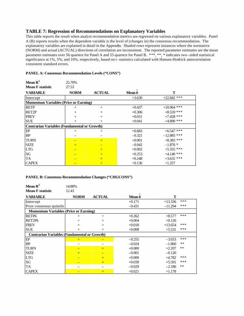
TABLE 7: Regression of Recommendations on Explanatory Variables This table reports the result when analyst recommendation metrics are regressed on various explanatory variables. Panel A (B) reports results when the dependent variable is the level of (changes in) the consensus recommendation. The explanatory variables are explained in detail in the Appendix. Shaded rows represent instances where the normative (NORM) and actual (ACTUAL) directions of correlation are inconsistent. The reported parameter estimates are the mean parameter estimates over 56 quarters for Panel A and 55 quarters for Panel B. ***, **, * indicates two–sided statistical significance at 1%, 5%, and 10%, respectively, based on t–statistics calculated with Hansen-Hodrick autocorrelation consistent standard errors. PANEL A: Consensus Recommendation Levels (“CONS”) Mean R2 25.70% Mean F statistic 27.53 VARIABLE NORM ACTUAL Mean

β T

Intercept +3.630 +22.842 *** Momentum Variables (Price or Earning) RETP + + +0.437 +10.964 *** RET2P + + +0.306 +8.559 *** FREV + + +0.031 +7.428 *** SUE + + +0.041 +4.890 *** Contrarian Variables (Fundamental or Growth) EP + + +0.683 +6.547 *** BP – – –0.321 –12.885 *** TURN – + +0.001 +8.383 *** SIZE + – –0.042 –1.876 * LTG – + +0.002 +5.355 *** SG – + +0.253 +4.140 *** TA – + +0.248 +3.632 *** CAPEX – + +0.136 +1.257

PANEL B: Consensus Recommendation Changes (“CHGCONS”) Mean R2 14.88% Mean F statistic 12.43

VARIABLE NORM ACTUAL Mean β T

Intercept +0.171 +13.336 *** Prior consensus quintile –0.431 –11.294 ***

Momentum Variables (Price or Earning) RETP6 + + +0.262 +8.577 *** RET2P6 + + +0.004 +0.126

FREV + + +0.018 +13.654 *** SUE + + +0.008 +5.531 ***

Contrarian Variables (Fundamental or Growth) EP + – –0.255 –3.033 *** BP – – –0.024 –1.860 ** TURN – + +0.000 +2.207 ** SIZE + – –0.001 –0.120

LTG – + +0.000 +4.782 *** SG – + +0.039 +5.591 *** TA – – –0.029 –2.186 **

CAPEX – + +0.021 +1.178

TABLE 8: Future Returns, Analyst Recommendations, and Investment Signals This table reports regressions of future returns on analyst recommendations and on various investment signals. Future returns are defined as the market–adjusted return in the six months after the month of the recommendation (RETF). Analyst recommendations used are: the quintile of the consensus recommendation level (QCON), and the quintile of the change in the consensus measured over the prior quarter (QCHGCON). QFITCON and QFITCHGCON are fitted values of QCON and QCHGCON from Panels A and B of Table 7, respectively. The reported parameter estimates are the mean parameter estimates from the quarterly regressions. ***, **, * indicates two–sided statistical significance at 1%, 5%, and 10%, respectively, based on t–statistics calculated with Hansen-Hodrick autocorrelation consistent standard errors. PANEL A: Consensus Recommendation Levels Quintiles (QCON)

Model A1 Model A2 Model A3 Model A4

Analysts

Alone Analysts &

QScore Analysts &

Binary Signals Analysts & Fitted Value

Parameter Estimate T-stat Estimate T-stat Estimate T-stat Estimate T-stat

Intercept -0.0257 -2.13** -0.0484 -2.79*** -0.0673 -2.65 ** -0.0336 -2.58** QCON 0.0226 1.83* 0.0108 1.22 0.0076 1.31 0.0074 1.42 QScore 0.0562 3.23*** QFITCON 0.0300 3.26*** RETP 0.0175 3.31 *** RET2P 0.0019 0.32 FREV 0.0324 17.99 *** SUE 0.0017 0.31 EP 0.0021 0.57 BP -0.0089 -1.41 TURN 0.0011 0.17 SIZE 0.0078 0.66 LTG 0.0007 0.11 SG 0.0007 0.44 TA 0.0268 9.46 *** CAPEX 0.0134 2.58 ** PANEL B: Consensus Recommendation Changes Quintiles (QCHGCON)

Model B1 Model B2 Model B3 Model B4

Analysts

Alone Analysts &

QScore Analysts &

Binary Signals Analysts & Fitted Value

Parameter Estimate T-stat Estimate T-stat Estimate T-stat Estimate T-stat

Intercept -0.0262 -1.85 * -0.0522 -2.86*** -0.0690 -2.64 ** -.0316 -1.96* QCHGCON 0.0225 5.26 *** 0.0190 3.80*** 0.0159 15.73 *** 0.0173 4.07*** QScore 0.0551 3.34*** QFITCHGCON 0.0159 2.75*** RETP 0.0176 3.51 *** RET2P 0.0014 0.31 FREV 0.0319 15.00 *** SUE 0.0027 0.52 EP 0.0011 0.61 BP -0.0080 -1.27 TURN 0.0000 0.00 SIZE 0.0065 0.56 LTG -0.0004 -0.06 SG 0.0002 0.10 TA 0.0261 10.18 *** CAPEX 0.0132 2.43 **

TABLE 9: Future Returns by Quantitative Scores and Analyst Recommendations This table reports the market-adjusted return in the six months following the recommendation. Firms are grouped by their quantitative measures (QScores) and consensus recommendations. Panels A, B, and C report results for the recommendation level quintiles (QCON), change quintiles (QCHGCON), and a combined strategy of level and change quintiles, respectively. ***, **, * indicate two-sided statistical significance at 1%, 5%, and 10%, respectively. PANEL A: Market–Adjusted Returns by Recommendation Level Quintile and QScore Quintile

Consensus Recommendation Level Quintile Worst=SELL: 0.00 0.25 0.50 0.75 1.00: Best=BUY

QScore Quintile Obs Mean Obs Mean Obs Mean Obs Mean Obs Mean BUY−SELL t p Worst=LOW 0.00 72.51 –0.0445 48.07 –0.0350 41.24 –0.0355 34.76 –0.0510 32.87 –0.0652 –0.0207 –1.37 0.25 42.51 –0.0318 31.33 –0.0250 29.93 –0.0269 30.55 –0.0275 29.09 –0.0358 –0.0040 –0.22 0.50 37.47 –0.0080 32.82 –0.0155 35.09 –0.0074 36.69 –0.0158 36.91 +0.0020 +0.0100 +0.58 0.75 26.67 –0.0049 28.49 –0.0131 35.96 –0.0080 38.29 +0.0101 34.85 +0.0226 +0.0276 +1.83** Best=HIGH 1.00 30.27 –0.0066 44.04 +0.0020 58.42 –0.0002 55.13 +0.0196 44.15 +0.0258 +0.0324 +3.30***

HIGH–LOW +0.0379 +0.0370 +0.0353 +0.0706 +0.0910 t +2.23 +2.73 +2.72 +4.77 +7.87 p *** *** *** *** ***

Overall analysts’ level recommendations = Buy−Sell (see also Table 3 Panel B) +0.0216 +1.66* Overall quantitative strategy = High−Low (see also Table 5 Panel B) +0.0541 +4.47*** DISAGREE = Low&Buy–High&Sell –0.0586 –4.03*** AGREE = High&Buy–Low&Sell +0.0703 +3.78*** PANEL B: Market–Adjusted Returns by Recommendation Change Quintile and QScore Quintile

Consensus Recommendation Change Quintile Worst=DECR: 0.00 0.25 0.50 0.75 1.00: Best=INCR

QScore Quintile

Obs Mean Obs Mean Obs Mean Obs Mean Obs Mean

Incr−Decr t p

Worst=LOW 0.00 59.42 –0.0623 29.65 –0.0270 72.49 –0.0553 25.02 –0.0368 39.84 –0.0326 +0.0297 +2.92*** 0.25 35.60 –0.0502 21.91 –0.0088 50.76 –0.0346 21.44 –0.0228 31.64 –0.0141 +0.0361 +4.55*** 0.50 33.82 –0.0229 25.44 –0.0043 55.36 –0.0138 26.36 –0.0053 35.93 +0.0022 +0.0251 +2.25** 0.75 28.33 –0.0035 25.65 –0.0033 47.55 +0.0041 26.38 +0.0040 34.60 +0.0112 +0.0148 +1.17 Best=HIGH 1.00 35.33 +0.0026 40.51 +0.0206 62.78 +0.0037 43.67 +0.0067 47.36 +0.0162 +0.0136 +1.83**

HIGH–LOW +0.0649 +0.0475 +0.0590 +0.0435 +0.0488 t +4.06 +2.55 +5.73 +2.86 +3.48 p *** *** *** *** ***

Overall Analysts’ change recommendations = Incr−Decr (see also Table 3 Panel C) +0.0268 +6.07*** Overall Quantitative strategy = High−Low (see also Table 5 Panel B) +0.0541 +4.47*** DISAGREE = Low&Incr–High&Decr –0.0352 –2.33*** AGREE = High&Incr–Low&Decr +0.0785 +5.29***

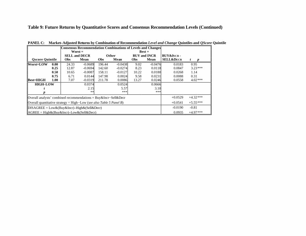
Table 9: Future Returns by Quantitative Scores and Consensus Recommendation Levels (Continued) PANEL C: Market–Adjusted Returns by Combination of Recommendation Level and Change Quintiles and QScore Quintile

Consensus Recommendation Combinations of Levels and Changes Worst =

SELL and DECR Other Best =

BUY and INCR Qscore Quintile Obs Mean Obs Mean Obs Mean

BUY&INCR − SELL&DECR t p

Worst=LOW 0.00 24.33 -0.0689 196.44 -0.0438 9.02 -0.0476 0.0183 0.95 0.25 12.87 -0.0694 142.60 -0.0274 8.23 0.0118 0.0847 3.23*** 0.50 10.65 -0.0087 158.11 -0.0127 10.22 0.0180 0.0268 1.14 0.75 6.71 0.0144 147.98 0.0024 9.58 0.0231 0.0088 0.31 Best=HIGH 1.00 7.07 -0.0319 211.78 0.0086 13.27 0.0246 0.0558 4.02***

HIGH–LOW 0.0374 0.0524 0.0666t 2.15 5.57 3.10p ** *** ***

Overall analysts’ combined recommendations = Buy&Incr−Sell&Decr +0.0529 +4.32*** Overall quantitative strategy = High−Low (see also Table 5 Panel B) +0.0541 +5.55*** DISAGREE = Low&(Buy&Incr)–High&(Sell&Decr) -0.0190 -0.81 AGREE = High&(Buy&Incr)–Low&(Sell&Decr) 0.0935 +4.97***

TABLE 10: Cumulative Excess Returns Over Various Holding Periods This table reports the market-adjusted returns over various holding periods following the recommendation. Firms are grouped by their quantitative measure (QScore, Momentum, Contrarian) and consensus recommendations. Panel A reports the mean difference in market-adjusted returns between the extreme consensus recommendation level quintiles (BUY-SELL) within each of the quantitative measure quintiles. Panels B repeats the analyses for changes in recommendations. ***, **, * indicate two-sided statistical significance at 1%, 5%, and 10%, respectively, based on t–statistics calculated with Hansen-Hodrick autocorrelation consistent standard errors. PANEL A: Mean market–adjusted return difference between extreme recommendation

level quintiles (BUY-SELL) within each quantitative quintile Within Quantitative Quintile

Holding Period Worst=LOW: 0.00 0.25 0.50 0.75

Best=HIGH: 1.00

Within QScore Quintile 1 month -0.0024 -0.0091 0.0045 0.0062 0.0071** 3 months -0.0051 -0.0014 0.0115 0.0223*** 0.0192*** 6 months -0.0207 -0.0040 0.0100 0.0276** 0.0324*** 9 months -0.0451** -0.0363* 0.0080 0.0415** 0.0448*** 12 months -0.0732*** -0.0390 -0.0038 0.0379 0.0502***

Within Momentum Quintile 1 month 0.0002 -0.0068 0.0006 0.0033 0.0054 3 months 0.0009 -0.0077 0.0031 0.0071 0.0262*** 6 months -0.0060 -0.0251** 0.0013 0.0083 0.0279*** 9 months -0.0198 -0.0468*** 0.0074 -0.0005 0.0380*** 12 months -0.0495 -0.0663*** 0.0004 0.0035 0.0363*

Within Contrarian Quintile 1 month 0.0005 0.0047 0.0045 0.0111*** 0.0057 3 months 0.0150 0.0169*** 0.0183*** 0.0284*** 0.0235*** 6 months 0.0041 0.0303*** 0.0255*** 0.0348*** 0.0474*** 9 months -0.0206 0.0226 0.0307** 0.0393** 0.0610*** 12 months -0.0446 0.0159 0.0259 0.0349 0.0695***

PANEL B: Mean market–adjusted return difference between extreme recommendation change quintiles (BUY-SELL) within each quantitative quintile

Within Quantitative Quintile Holding Period Worst=LOW:

0.00 0.25 0.50 0.75 Best=HIGH:

1.00 Within QScore Quintile

1 month 0.0108*** 0.0087*** 0.0095*** 0.0065** 0.0062** 3 months 0.0166*** 0.0213*** 0.0156*** 0.0088 0.0114*** 6 months 0.0297*** 0.0361*** 0.0251*** 0.0148 0.0136** 9 months 0.0280*** 0.0528*** 0.0309*** 0.0253* 0.0186*** 12 months 0.0208 0.0511*** 0.0323** 0.0356*** 0.0245***

Within Momentum Quintile 1 month 0.0016 0.0129*** 0.0122*** 0.0090*** 0.0038 3 months 0.0114* 0.0156*** 0.0144*** 0.0164*** 0.0119* 6 months 0.0257*** 0.0251*** 0.0337*** 0.0214*** 0.0166 9 months 0.0264*** 0.0368*** 0.0459*** 0.0223*** 0.0325*** 12 months 0.0124 0.0276 0.0448*** 0.0346*** 0.0463***

Within Contrarian Quintile 1 month 0.0183*** 0.0043 0.0072*** 0.0092*** 0.0106*** 3 months 0.0309*** 0.0132** 0.0165*** 0.0067 0.0165*** 6 months 0.0450*** 0.0313** 0.0170*** 0.0137 0.0288*** 9 months 0.0522*** 0.0292*** 0.0330*** 0.0297*** 0.0260*** 12 months 0.0624*** 0.0269** 0.0240** 0.0336*** 0.0322***

FIGURE 1: Data accumulation periods relative to portfolio formation date

PANEL A: Dependent variables: Consensus level and change in consensus

Accumulation over 12 months

Two day window preceding tCurrent consensus recommendation level Ò

Accumulation over 12 months

Two day window preceding t-1Prior consensus recommendation level Ò

changeChange in consensus recommendation

PANEL B: Independent variables: Investment signals

Months –6 to 0

ÒAnalyst-based:FREV and LTG

Market-based:RETP, RET2P,TURN, and SIZE

Months –12 to – 7 Months –6 to – 1

Ò

Accounting-based:

Rolling sum of 4 qtrs

Max 4 qtr preceding periodTwo month window preceding tq = most recent quarter

for which earnings announcement made

t+1t–1t–4 t–3 t–2t–5 t+2 t+3 t+4 t+5Preceding6 months

begins

Precedingyear begins

Subsequentyear ends

Subsequent6 months

ends

Consensust

Quarter-end: t–8 t–7 t–6t–92nd precedingyear begins

SUE, SG, CAPEX, TA, EP, and BP

Deflator for selected variables incorporates 2nd preceding year info

q

FIGURE 2. Cumulative Excess Returns to Analyst Recommendation Strategies (Level and Change) in Combination

with Quantitative Quintiles

PANEL A: Consensus Recommendation Levels Quintiles (QCON), Separately and in Combination with Quantitative Quintiles (QScore)

0.0120.0190.0220.016

0.004

0.0680.0730.070

0.044

0.017

0.000

0.010

0.020

0.030

0.040

0.050

0.060

0.070

0.080

0.090

0.100

1 month 3 months 6 months 9 months 12 months

Mea

n E

xces

s R

etur

ns

QSCORE: High-Low ANALYSTS: Buy-Sell COMBINED: High/Buy-Low/Sell

PANEL B: Consensus Recommendation Changes Quintiles (QCHGCON), Separately and in Combination with Quantitative Quintiles (QScore)

0.0360.0350.027

0.017

0.009

0.077

0.091

0.079

0.048

0.025

0.000

0.010

0.020

0.030

0.040

0.050

0.060

0.070

0.080

0.090

0.100

1 month 3 months 6 months 9 months 12 months

Mea

n E

xces

s R

etur

ns

QSCORE: High-Low ANALYSTS: Incr-Decr COMBINED: High/Incr-Low/Decr

PANEL C: Consensus Recommendation Levels Quintiles (QCON) and Changes Quintiles (QCHGCON), Separately and in Combination with Quantitative Quintiles (QScore)

0.0560.063

0.053

0.028

0.015

0.069

0.0910.093

0.055

0.027

0.000

0.010

0.020

0.030

0.040

0.050

0.060

0.070

0.080

0.090

0.100

1 month 3 months 6 months 9 months 12 months

Mea

n E

xces

s R

etur

ns

QSCORE: High-Low ANALYSTS: Buy/Incr-Sell/Decr COMBINED: High/Buy/Incr-Low/Sell/Decr

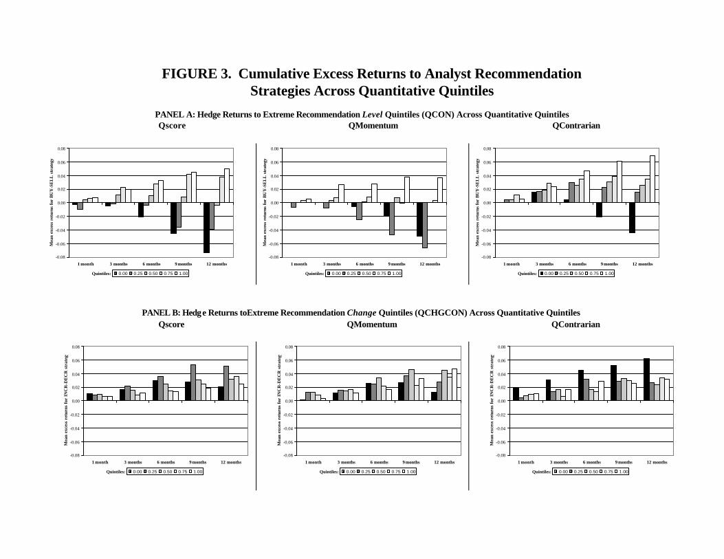
FIGURE 3. Cumulative Excess Returns to Analyst Recommendation Strategies Across Quantitative Quintiles

PANEL A: Hedge Returns to Extreme Recommendation Level Quintiles (QCON) Across Quantitative Quintiles Qscore QMomentum QContrarian

-0.08

-0.06

-0.04

-0.02

0.00

0.02

0.04

0.06

0.08

1 month 3 months 6 months 9 months 12 months

Mea

n ex

cess

ret

urns

for

BU

Y-S

EL

L s

trat

egy

0.00 0.25 0.50 0.75 1.00Quintiles:

-0.08

-0.06

-0.04

-0.02

0.00

0.02

0.04

0.06

0.08

1 month 3 months 6 months 9 months 12 monthsM

ean

exce

ss r

etur

ns f

or B

UY

-SE

LL

str

ateg

y

0.00 0.25 0.50 0.75 1.00Quintiles:

-0.08

-0.06

-0.04

-0.02

0.00

0.02

0.04

0.06

0.08

1 month 3 months 6 months 9 months 12 months

Mea

n ex

cess

ret

urns

for

BU

Y-S

EL

L s

trat

egy

0.00 0.25 0.50 0.75 1.00Quintiles:

PANEL B: Hedge Returns toExtreme Recommendation Change Quintiles (QCHGCON) Across Quantitative Quintiles Qscore QMomentum QContrarian

-0.08

-0.06

-0.04

-0.02

0.00

0.02

0.04

0.06

0.08

1 month 3 months 6 months 9 months 12 months

Mea

n ex

cess

ret

urns

for

IN

CR

-DE

CR

str

ateg

y

0.00 0.25 0.50 0.75 1.00Quintiles:

-0.08

-0.06

-0.04

-0.02

0.00

0.02

0.04

0.06

0.08

1 month 3 months 6 months 9 months 12 months

Mea

n ex

cess

ret

urns

for

IN

CR

-DE

CR

str

ateg

y

0.00 0.25 0.50 0.75 1.00Quintiles:

-0.08

-0.06

-0.04

-0.02

0.00

0.02

0.04

0.06

0.08

1 month 3 months 6 months 9 months 12 months

Mea

n ex

cess

ret

urns

for

IN

CR

-DE

CR

str

ateg

y

0.00 0.25 0.50 0.75 1.00Quintiles: