1

Analyzing Taiwan’s Air Pollution: An Application of the CGE Model and the Concept of Green National Product

Yun-Peng Chu*, Shih-Mo Lin**, and Ching-Wei Kuo***

Abstract

The purposes of this paper are to establish a link between the concept of green national product and that of CGE modeling, and demonstrate empirically the existence of significant differences between the value of conventional GNP and that of Green GNP. We first derive theoretically the framework of Green GNP under two different definitions, SEEA and ENRAP, taking into account pollution and pollution prevention activities. Then, we employ a 28-sector static CGE model for Taiwan to assess the effects of the policy of mandatory reduction in air pollution emission on Taiwan’s macroeconomic variables as well as sectoral resource allocation. The social accounting matrix used by the CGE model is compiled on the basis of the 1997 national income data (aggregates) and 1996 input-output data (structure). The model is then supplemented by the pollution generation coefficients, the emission coefficients and the abatement costs, which are computed from the Trial Compilation of Green National Product prepared by the Directorate-General of Budgeting, Accounting, and Statistics (DGBAS). Three kinds of air pollutants are considered: Sulfur Oxides (SOx), Nitrogen Oxides (NOx), and Volatile Organic Compounds (VOC). Simulation results generated from the model are used to compute two measures of Green National Product, the EDPII under the United Nations’ SEEA system, and an alternative measure, which is derivable from maximizing the present value of future consumption stream and is closer to the ENRAP system, in addition to the conventional GNP and other macroeconomic and sectoral variables. It is found that although a more stringent air pollution control policy will raise costs and thereby reduce the conventional GNP, the Green National Product, which reflects social welfare better than the conventional GNP does, will increase by either measure. Sectorally, industries with heavier air pollution generations tend to lose resources to the other sectors, as expected. *Research Fellow, ISSP, Academia Sinica and Professor of Industrial Economics, National Central University. **Professor of International Trade, Chung Yuan Christian University. ***Associate Research Fellow, ITRI, Taiwan.

2

Analyzing Taiwan’s Air Pollution: An Application of the CGE Model and the Concept of Green National Product

Yun-Peng Chu1, Shih-Mo Lin2, and Ching-Wei Kuo3

1. Introduction

The concept of Green NDP differs from that of traditional NDP by accounting for the

parts of depletion in natural resources and degradation of the environment, which are not

included in the computation of the traditional NDP. As such, it is closer to the social welfare

concept in economics than is traditional NDP. It is therefore a more preferable goal of

policies. Since the publication of SEEA (1993) by the United Nations, many institutions and

countries have involved in studying and implementing the construction of Green Domestic

Product, including the United Nations, Japan, Korea, and so on.

The government of Taiwan has already devoted to the Trial Compilation of Green NDP

since 2000 (DGBAS, 2000). Taiwan’s construction is based on the method recommended by

SEEA (1993). As such, it leaves at least two rooms for improvement. One is to take into

account the effect suggested by Aaheim and Nyborg (1995). Aaheim and Nyborg point out

that the SEEA framework subtracts the monetary degradation called “maintenance cost”

associated with untreated pollution from the Traditional Net Domestic Product, as if the

imputation of this monetary amount and the traditional NDP are independent of each other. In

the real world, if government policies require large reduction in the untreated wastes, the

private sector will change their behavior. So the traditional NDP would not be independent of

the changing policy, and that is why Aaheim and Nyborg stressed the importance of taking

the general equilibrium aspect into consideration when compiling Green NDP. The above is

1 Research Fellow, ISSP, Academia Sinica and Professor of Industrial Economics, National Central University. 2 Professor of International Trade, Chung Yuan Christian University. 3 Associate Research Fellow, ITRI, Taiwan.

3

the first reason why we write this paper. Specifically, this paper uses a general equilibrium

model to catch the inter-sectoral and macroeconomic effects of tighter air pollution control

policies and then compute Green NDP based on the simulation results of the model.

The second reason for improvement, as Chu (2000) points out, is that maintenance cost

as defined by SEEA (1993) is actually the “benefits” of environmental pollution. In a

theoretically correct formulation of Green NDP, as developed by Chu (2000), such benefits

should not be subtracted, where should be subtracted from Traditional NDP is the “cost” of

“environmental pollution”.

The new draft handbook of Green National Product prepared by the London Group has

taken this point into account. So they define a new measure of Green NDP, among many

other options, which subtracts damages of pollution rather than the benefits of pollution from

traditional NDP. And this is the second reason and contribution of our paper, because this

paper will compute not only the SEEA (1993) Green NDP, but also an alternative Green NDP,

which subtracts damages of air pollution from traditional NDP rather than the maintenance

cost. We will call this new measure Revised Green NDP.

In what follows, we will review some related literature in section 2, explain the

theoretical framework in section 3, and describe the modeling inputs in section 4. Section 5

gives the figures, and finally concluding remarks are given in section 6.

2. Review of literature (1) Air pollution: CGE studies

Conrad and Schroder (1993) use a dynamic CGE model to assess the impact on

economy of difference kinds of environmental policy tools, and it is found that the

imposition of emission fee is the first best policy, while the second best policy be subsidizing

the pollution abatement activities by the firms. Bergman (1990) uses a CGE model to assess

4

the effects of nuclear power policies on GNP and the sectoral allocation of resources. Its

model contains 45 sectors and covers the period of 1985 to 2000. It is found that if policies

are undertaken to reduce the SOx and NOx emission from the 1980 base level, the Swedish

GNP will be reduced substantially.

Xie (1996) uses a CGE model to assess the impact of a wastewater emission fee on the

economy of China. He found that an increase in tax rate will result in a reduction of domestic

product, an increase in price and unemployment, but a decrease in pollution emissions. Yang

(2001) uses a 18-sector CGE model to assess the effects of trade liberalization on the

emission of CO2 in Taiwan, and found that trade liberalization will result in an increase in

total CO2 emission. In addition, resources will flow from low to high carbon content

products.

Wiebelt (2001) uses an open economy CGE model to assess the effects of

environmental tax on hazardous waste in South African mining industry. It is found that the

imposition of tax will increase the production cost, lowering the international

competitiveness of the mining products. In addition, the miners will be adversely affected.

Abimanyu (2000) uses a CGE model called INDORANI to simulate the effects of reducing

agriculture trade distortion and government subsidy on economic and environmental

variables. It is found that although the effect on GDP is positive, the environment will be

adversely affected.

Garbaccio, Ho, and Jorgenson (1999) construct a dynamic CGE model for China to

assess the effects of carbon taxation. They found that under the neutral carbon taxation policy,

China could achieve the “double dividend” effect. Morris, et al. (1999) use a CGE model

called FEIM to assess the effects of air pollution tax on the economy of Hungary, but their

results show that the double dividend effect would not be significant.

Lai and Wang (1997) use a 13-sector CGE model to assess the effects of tighter air

pollution control policies on the petroleum chemical industry and some macroeconomic and

5

sectoral variables. It is found that because the enterprises have to devote more resources to

pollution control, the real GDP will be adversely affected. Chiang (1995) uses a CGE

model to assess the effects of end-of-pipe air pollution control policies on Taiwan’s

macroeconomic and sectoral variables. He takes into account the operation as well as the air

pollution control equipment investment expenditure and finds that the increase in operation

and maintenance cost will result an increase in prices, resulting in a decrease in GDP and

total output. On the other hand, the increase in air pollution control equipment investment

will have much smaller effects.

All the above studies are very useful for the problems concerned with, and have all been

able to catch the general equilibrium effects of policy changes. But so far there has not seen

to be any CGE model that involves in the computation of Green NDP. So our paper will be

CGE-based and involved in the computation of Green NDP at the same time.

(2) Green GDP Studies

Adjustments of conventional national product measures to reflect changes in the value

of environmental assets, popularly known as green accounting, have gained considerable

attention in recent years. In the U.S., intensive work on environmental accounting began in

the Bureau of Economic Analysis (BEA) of the U.S. Department of Commerce in 1992.

Shortly after the first publication of the U.S. Integrated Environmental and Economic

Satellite Accounts (IEESA) in 1994, however, Congress directed the Commerce Department

to suspend further work in this area and to obtain an external review of environmental

accounting. A panel was then organized by the National Research Council and charged to do

the work. The final report of the panel was recently released (Nordhaus and Kokkelenberg,

1999). There the panel concludes that “extending the U.S. national income and product

accounts to include assets and production activities associated with natural resources and the

environment is an important goal; and that developing a set of comprehensive non-market

6

economic accounts is a high priority for the nation.” The panel explicitly recommends that

“Congress authorize and fund Bureau of Economic Affairs of the Department of Commerce

to recommence its work on developing natural-resource and environmental accounts.”

Elsewhere the work continued without pause in many countries.4

3. Methodology 3.1 CGE Model

This paper uses a revised version of the DMR model, in which a total of 28 sectors are

included. The entire equation system is shown in Table 1, it includes the price determination,

production, income, consumption, saving, market clearing, environmental and air pollution

equations. This section will only explain in more details the part of equations that are directly

associated with air pollution, because the other specifications are pretty standard.

(1) Production function

iiiii

ji

jii

jijji

jiji

jijji

jiii

ji

jii

jijji

jiji

jijji

jiiii

LKAXTHETANAANTDC

AANTGCNTUABCTHETANAANCPCAAAANLPG

AANFOCAANDCAANGCAAAANNGC

AANCCNPOSTCNUABCTHETASAASTDC

AASTGCSTUABCTHETASAASCPCAAAASLPG

AASFOCAASDCAASGCAAAASNGC

AASCCSPOSTCSUABCX

αα−⋅−⋅⋅+

⋅⋅−−⋅⋅++⋅+

⋅+⋅+⋅++⋅+

⋅+⋅−−⋅⋅+

⋅⋅−−⋅⋅++⋅+

⋅+⋅+⋅++⋅+

⋅+⋅−=

1,10

,9

,13,24,12

,11,10

,9,24,3

,2

,10

,9

,13,24,12

,11,10

,9,24,3

,2

)))1()957563456.09992786733.0((

))1())597089127.0(042436543.0

70007291326.0)40291087.0(((

))1()957563456.09992786733.0((

))1())597089127.0(042436543.0

70007291326.0)40291087.0(((1(

(1)

Where,

Xi = sectoral domestic output

4 See the survey in Peskin (1999). For recent efforts by Japan and Korea along the United Nation’s System of Integrated Environmental and Economic Accounting or SEEA (CECE et. al, 1993, and UN, 1998) line, see Economic Planning Agency, Japan, 1998, and UNDP, 1998; and for efforts along the ENRAP (Environmental and Natural Resources Accounting Project as implemented in the Philippines) line, see IRG, 1996.

7

AXi = technology parameter (constant of production function)

Ki = sectoral capital stock

Li = sectoral labor demand

αi (alpha) = labor share

AAji = input-output coefficient

SPOSTCi and NPOSTCi:= SOx and NOx process emission factor respectively

SCCi (NCCi) = SOx (NOx) combustion emission factor associated with coal

SNGCi (NNGCi) = SOx (NOx) combustion emission factor associated with natural gas

SGCi (NGCi) = SOx (NOx) combustion emission factor associated with gasoline

STGCi (NTGCi)= SOx(NOx) combustion emission factor associated with gasoline

SDCi (NDCi) = SOx(NOx) transportation emission factor associated with diesel

STDCi (NTDCi) =SOx(NOx) transportation emission factor associated with diesel

SFOCi (NFOCi) = SOx (NOx) combustion emission factor associated with fuel oil

SLPGCi (NLPGCi) = SOx (NOx) combustion emission factor associated with liquid petroleum gas

SCPCi (NCPCi) = SOx(NOx) combustion emission factor associated with coal products

SUABCi (NUABCi)= SOx (NOx) unit abatement cost

STUABCi (NTUABCi) = SOx (NOx) unit abatement cost of transportation pollution

THETAS (THETAN) = SOx (NOx) emission-reduced rate (air control policy)

According to many studies including Liu (1999), Gray and Shadbegian (1993), Barbera

and McConnell (1990), and Conrad and Wastl (1995), tighter environmental control typically

will result in higher cost. Although there have been examples of tighter pollution control

result in higher productivity, such as Royston (1979), but evidence are spare and may involve

some information asymmetry.

So in this paper we will still adopt the standard assumption, that is, tighter control will

result in higher cost. Specifically, the pollution control activities are specified as having an

effect on the technology parameter of the production function. So, when the sector is required

by new policy to adopt tighter control, the technology parameter AXi would be multiply by

8

))1()(1( b

b

XTHETAPOSTCXUABC −⋅⋅

− , where UABC is unit abatement cost, POCTC is process

emission factor, Xb is sectoral domestic output in baseline, and THETA is emission-reduced

rate associated with air control policy.

There are many kinds of air pollutants, but not all of them have sufficient data to justify

the inclusion in the model. So in this paper we will only consider Sulfur Oxides (SOx) and

Nitrogen Oxides (NOx). The parameter used in the study are POSTC, UABC, THETA,

sectoral process emission, sectoral combustion emission, and etc. Combustion emission can

be further divided into two parts, one is combustion associated with production, and the other

is transportation emission.

To compute combustion emission, we first compute the different type of fuels used in

the production and transportation process by the various sectors. These fuels include gasoline,

diesel, fuel oil, natural gas, coal and coal products. All six types are used in production, but

only gasoline and diesel are used in transportation.

(2) Environmental equations

(2.1) Sectoral process emission�

THETASSPOSTCXSOxMQU iii ⋅⋅= (2)

THETANNPOSTCXNOxMQU iii ⋅⋅= (3)

Where SOxMQUi and NOxMQUi are sectoral SOx and NOx process emission. The definition of the other variables is the same with production function.

(2.2) Sectoral combustion and transportation emission�

THETASAASCPCAAAASLPGAASFOCAASTDCAASDC

AASTGCAASGCAAAASNGCAASCCXSOxF

jijjiji

jiji

jiji

jjijiii

⋅⋅++⋅+⋅+⋅+⋅+⋅+⋅+

+⋅+⋅=

))597089.0(957563456.0042436543.0

39992708673.070007291326.0)402910872.0((

,13,24,12,11

,10,10

,9,9

,24,3,2

9

(4)

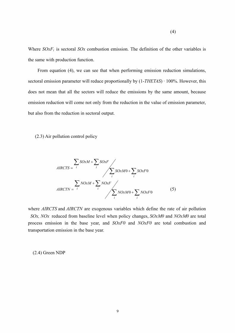
Where SOxFi is sectoral SOx combustion emission. The definition of the other variables is

the same with production function.

From equation (4), we can see that when performing emission reduction simulations,

sectoral emission parameter will reduce proportionally by (1-THETAS) · 100%. However, this

does not mean that all the sectors will reduce the emissions by the same amount, because

emission reduction will come not only from the reduction in the value of emission parameter,

but also from the reduction in sectoral output.

(2.3) Air pollution control policy

∑∑∑∑

+

+

=

ii

iiSOxFSOxM

SOxFSOxMAIRCTS

00

∑∑∑∑

+

+

=

ii

iiNOxFNOxM

NOxFNOxMAIRCTN

00 (5)

where AIRCTS and AIRCTN are exogenous variables which define the rate of air pollution�SOx, NOx�reduced from baseline level when policy changes, SOxM0 and NOxM0 are total process emission in the base year, and SOxF0 and NOxF0 are total combustion and transportation emission in the base year.

(2.4) Green NDP

10

⋅⋅⋅+

⋅⋅⋅⋅+

⋅⋅⋅−

⋅⋅⋅−+

⋅

−

⋅⋅⋅+

⋅⋅⋅⋅+

⋅⋅⋅−

⋅⋅⋅−+

⋅

−−=

∑

∑

∑

∑

i iii

iiii

iiii

iii

ixix

i

i iii

iiii

iiii

iii

ixix

i

LTHETANNTDCAALX

LTHETANNTGCAALXNTUABC

LTHETANNTDCAALX

LTHETANNTGCAALXLFNOLMNO

NUABC

LTHETASSTDCAALX

LTHETASSTGCAALXSTUABC

LTHETASSTDCAALX

LTHETASSTGCAALXLFSOLMSO

SUABC

LTDEPRLRGDPSGNDP

.95756.0.

.99927.0.

.95756.0.

.99927.0...

.95756.0.

.99927.0.

.95756.0.

.99927.0...

..

,10

,9

,10

,9

,10

,9

,10

,9

�6�

( ) ( )

+⋅++⋅⋅−−= ∑∑

iixix

iixix LFNOLMNOLFSOLMSOLTDEPRLRGDPRGNDP ..000172.0..0035.02757.18..

�7�

Equations (6) and (7) described above are the SEEA (1993) Green NDP and an alternative, revised measure of damage based Green NDP. The last term of the RHS of equation (6) is total maintenance cost, and the last term of equation (7) is total damage cost.

(3) Assumptions

(3.1) Domestic products and imports are imperfect substitutes. The domestic composite

goods supply (Qi) is a CES function of domestic production (Di) and Imports.

(3.2) Domestic products and Exports are perfect substitutes.

(3.3) Exchange rate is fixed.

(3.4) The current model is static, so sectoral capital stocks are exogenously given and

fixed.

3.2 Green GDP Model

Given the growing importance of green accounting, there are unfortunately still clouds

11

of doubts around it both theoretically and empirically. Here we attempt to clarify some of the

concepts concerning the treatment of important variables including defensive spending,

direct service of environment, and depreciation in the process of constructing the green

national product. It will be done by comparing both the United Nations’ SEEA (System of

Integrated Environmental and Economic Accounting) and the Philippine ENRAP

(Environmental and Natural Resources Accounting Project) framework (closely associated

with Professor Henry Peskin5) with a theoretically ideal system of national product, which

the paper will build as an extension of the Hamilton’s (1994, 1996) analysis.6

In particular, Hamilton’s Models 2 and 5 in his 1996 paper as well as some parts of Model 1 in his 1994 paper will be integrated into one model, which will subsequently be transformed and re-interpreted. The idea is to develop a formulation that is as simple as possible, but powerful enough to address the issues at hand. It will be clear that the model to be presented is enough for the purpose, and possible extensions of the model to include other aspects such as exhaustible resources would be intuitive.

(1) The Model

Mostly following Chu (2000), the following symbols are defined:

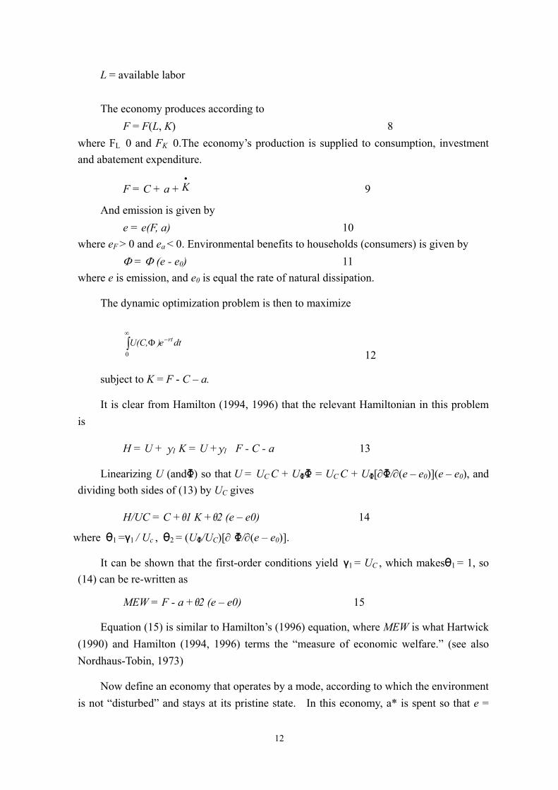
U = utility C = consumption K = capital stock (produced assets) F = production g = net natural growth of resource d = dissipation rate of the stock of pollution e = pollution emissions a = abatement expenditure by producers Φ = environmental benefits to households

5 For an earlier work on the comparison between SEEA and ENRAP that is from ENRAP’s viewpoints, see Peskin and delos Angeles, 1998. 6 Weitzman (1976) shows that the present value of future consumption would be maximized by maximizing in each period the “national product” as conventionally defined, if the economy is on the dynamically optimal path. Solow (1986) subsequently shows that national product can be conceived as the interest on total accumulated wealth, and is followed by Usher (1994) who shows the Hamiltonian in the dynamic optimization specification is the return to wealth, defined as the present value of future consumption. Hartwick (1990), Mäler (1991) both extends Weitzman’s model to analyze different aspects of the problem, while Hamilton (1994, 1996) attempts to synthesize and integrate the analysis by presenting a series of models that touch upon almost all of the important aspects of concern.

12

L = available labor

The economy produces according to F = F(L, K) �8�

where FL�0 and FK�0.The economy’s production is supplied to consumption, investment and abatement expenditure.

F = C + a +•

K �9�

And emission is given by e = e(F, a) �10�

where eF > 0 and ea < 0. Environmental benefits to households (consumers) is given by Φ = Φ (e - e0) �11�

where e is emission, and e0 is equal the rate of natural dissipation.

The dynamic optimization problem is then to maximize

dte)U(C, rt−∞

∫ Φ0 �12�

subject to K �= F - C – a.

It is clear from Hamilton (1994, 1996) that the relevant Hamiltonian in this problem is

H = U + γ1 K� = U +γ1�F - C - a� �13�

Linearizing U (andΦ) so that U = UC C + UΦΦ = UC C + UΦ[∂Φ/∂(e – e0)](e – e0), and dividing both sides of (13) by UC gives

H/UC = C +θ1 K �+θ2 (e – e0) �14�

where θ1 =γ1 / Uc , θ2 = (UΦ/UC)[∂ Φ/∂(e – e0)].

It can be shown that the first-order conditions yield γ1 = UC , which makesθ1 = 1, so (14) can be re-written as

MEW = F - a +θ2 (e – e0) �15�

Equation (15) is similar to Hamilton’s (1996) equation, where MEW is what Hartwick (1990) and Hamilton (1994, 1996) terms the “measure of economic welfare.” (see also Nordhaus-Tobin, 1973)

Now define an economy that operates by a mode, according to which the environment is not “disturbed” and stays at its pristine state. In this economy, a* is spent so that e =

13

(F* , a*) = d = e0.

Variables at such a hypothetical state have been denoted by an asterisk. Now we define the “sustainable” green NNP as gNNP* = F* - a*

“Regular” green NNP (called “MEW”) can then be defined as gNNP* plus deviations (called “Vi’s”) from that mode of activities:

MEW = gNNP = gNNP* + Σi=1,2Vi �16�

V1 is what the actual abatement expenditure falls short of a*, the level at which the environment would not be “disturbed.” So this means the money firms save when they use the environment as a dumping place beyond natural dissipation levels. It therefore measures the additional service of the environment to producers who dispose of their wastes in the environment in excess of the natural absorptive capacity. The term V2 is the remaining cost borne by consumers due to the fall in environment even after taking defensive actions.

So the sum of terms V1 and V2 actually represent the “net benefits” to an economy when it deviates from the “clean” or “sustainable” mode of production, i.e., it is the “net benefits of deviation.”

Turn now to the question of conventional NNP. Hamilton defines conventional NNP as total production, F (Hamilton, 1996, p. 22), and argues in his Model 2 that a should be deducted because it is actually an “intermediate consumption.” We will here simply make the assumption that either a has been recorded as an intermediate consumption (and so is not part of conventional NNP), or that it has been otherwise imputed as such and deducted. By so doing, we will define conventional NNP as F - a. We will call conventional NNP so defined “cNNP.”

Now let us give green NNP an alternative interpretation. Under the sustainable mode, cNNP* = F* - a* = gNNP*

It would be useful to examine the relationship among cNNP*, gNNP and cNNP. Let us then re-write equation (16)

MEW = gNNP = gNNP* + Σi=1,2Vi = cNNP* + Σi=1,2Vi

= cNNP* + (cNNP – cNNP*) +θ2 (e – e0) �17�

That is, when the environment is brought back into the picture, benefits V1 (waste disposal) would have been recorded by the conventional NNP. But conventional NNP is obviously an unsatisfactory candidate to maximize, because the term V2 is left out. And this is precisely why the green accounting exercise is valuable.

14

(2) The SEEA and Revised Approaches and the Green NDP

SEEA (Version IV.2 in 1993, 1998) defines gNNP as cNNP minus “depletion” and “degradation” of natural resources. The depletion is estimated at net rent cost, or at user-cost, while degradation is estimated at the hypothetical abatement cost of bringing down pollution from the existing (post-treatment) level to a level that does not harm the environment (called “maintenance cost”).

ENRAP has the “factor cost” and the “expenditure” side of the accounts. On the former side, gNNP equals cNNP plus waste disposal services (a negative number, as it is seen as a “subsidy” from nature) plus “net environmental benefits” minus “depreciation of ‘natural assets’ such as minerals, forests and fishery.”7 On the latter side, gNNP equals cNNP minus environmental damages (workday loss and medical costs) plus direct services of the environment to consumers minus “depreciation of natural assets.”

Imputed the SEEA (1993) gNNP and the Revised gNNP, our model ignored the depletion of natural resources and direct services of the environment.

4. Input Data The model uses the 1997 National Income as the main input of data. Basically, all

aggregate figures are taken from that publication, but sectoral distribution is based on the

1996 Input-Output Tables. The pollution-related variables including the emission factors and

the abatement cost are based on various research reports from the Environmental Protection

Agency. The estimation of air pollution damages is based on Liang (1993). The specific steps

of compilation is explained as follows:

(1) The dose response function of respiratory disease resulting from SOx and NOx air

pollution are as follows:

NOx : 9.03875 * 10-6 (per person per day/PPb)

SOx : 1.42133 *10-4 (per person per day /PPb)

(2) Using the emission factors (Table 10) to compute the amount of air pollution resulting

from various energy consumption.

15

(3) Linking the air pollution concentration indicators to total emissions. The method is based

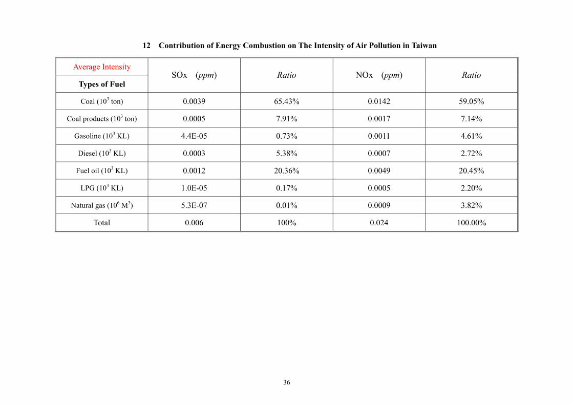
on Liang (1993), but the data have been updated. The results are shown in Table 12.

(4) Using the Shaw et al. (1992) results to assess the avoidance cost. Based on their study, the

average person in Taiwan is willing to pay NT$450 per day for the avoidance of the

disease in 1992. We multiply this figure by the consumer price index to get the 1997

amount of NT$520.10.

(5) Unit damage (private health cost per unit of air pollution emission) equals concentration

ratio times probability of disease, times population, then times private health cost per

instance of disease.

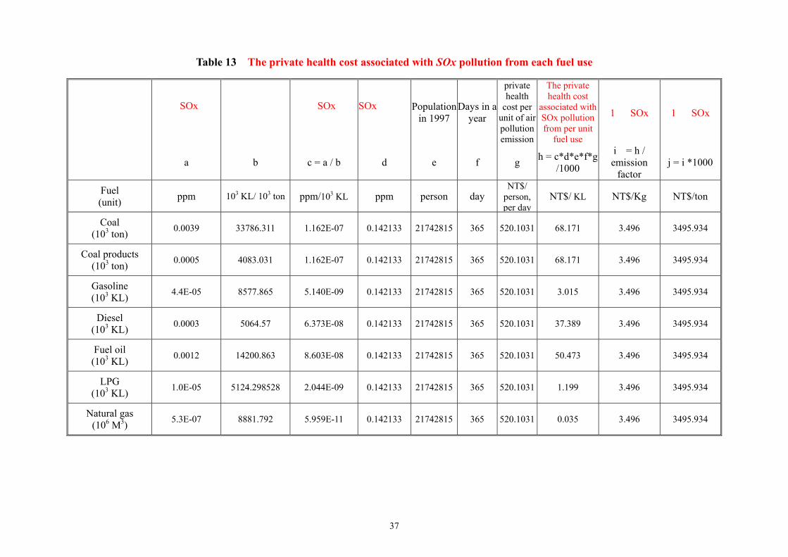
And this can be further specified according to different types of fuel use, as follows.

�1�The private health cost associated with SOx pollution per unit coal used:

= (ton

ppm310311.33786

003925958.0 ) * ( 0.142133 / ppm) * 21742815 persons * 365 days *

520.1031 NT$/per person, day = 68170.71959�NT$/per 103 ton�

�2�The private health cost associated with SOx pollution per unit coal products used:

= (ton

ppm310031.4083

000474447.0 ) * ( 0.142133 / ppm) * 21742815 persons * 365 days

*520.1031 NT$/per person, day

= 68170.71959�NT$/per 103 ton�

�3�The private health cost associated with SOx pollution per unit gasoline used:

= (KL

ppm310865.8557

0000440868.0 ) * ( 0.142133 / ppm) * 21742815 persons * 365 days

*520.1031 NT$/per person, day

= 3015.24337�NT$/per 103 KL�

�4�The private health cost associated with SOx pollution per unit diesel used:

= (KL

ppm31057.5064

00032277.0 ) * ( 0.142133 / ppm) * 21742815 persons * 365 days

*520.1031 NT$/per person, day

7 Imputed household production is included in ENRAP but ignored here for simplicity.

16

= 37389.01774�NT$/per 103 KL�

�5�The private health cost associated with SOx pollution per unit fuel oil used:

= (KL

ppm310863.14200

001221735.0 ) * ( 0.142133 / ppm) * 21742815 persons * 365 days

*520.1031 NT$/per person, day

= 50472.55200�NT$/per 103 KL�

�6�The private health cost associated with SOx pollution per unit LPG used:

= (KL

ppm310298528.5124

0000104737.0 ) * (0.142133/ ppm) * 21742815 persons * 365 days

*520.1031 NT$/per person, day

= 1199.10548�NT$/per 103 KL�

�7�The private health cost associated with SOx pollution per unit natural gas used:

= (3610792.8881

620000005292.0

m

ppm ) * ( 0.142133 / ppm) * 21742815 persons * 365 days

*520.1031 NT$/per person, day

= 34.95934�NT$/per 106 m3�

The private health cost associated with NOx pollution is computed by similar methods,

and will not be repeated here. It is worth noting, however, that private health cost is not the

only cost associated with air pollution. Typically, the deterioration in health will also incur a

substantial amount of external cost. Liang (1993) computes the external cost and concludes

the total social cost should be 18.2757 times the private health cost. Therefore, we use this

multiplier to derive the total social cost of health damage associated with SOx and NOx

pollution.

5. Scenarios and Analysis

(1) Scenarios

In addition to the baseline, our model computes the effects of three different scenarios as

shown in the following table.

17

Scenarios Definition

Scenario 1 Economy-wide SOx and NOx emissions are reduced by 10% from baseline. Unit abatement cost is unchanged. (See Table 9)

Scenario 2 Economy-wide SOx and NOx emissions are reduced by 20% from baseline. Unit abatement cost is unchanged. (See Table 9)

Scenario 3 Economy-wide SOx and NOx emissions are reduced by 20%, but unit abatement cost is 1.2 times the baseline level.

Scenario 3 is designed to reflect the possibility that as the mandatory reduction in air

pollution becomes more stringent, firms have to pay higher abatement cost than before,

according to the concept of an increase in abatement cost.

(2) Macroeconomic effects

Table 15 reports the macroeconomic effects of baseline and three scenarios. It shows

that domestic total output will be reduced by 0.009%, 0.018% and 0.019% respectively under

the three scenarios. GDP will be reduced by 0.007%, 0.013% and 0.015% respectively under

the three scenarios, while total labor compensation will be decreased by 0.014%, 0.028% and

0.033% respectively under the three scenarios.

There will be deterioration in trade surplus as exports fall and imports rise under the

three scenarios. These results are due mainly to the effects of domestic price rise as a result

of tighter air pollution control policies.

(3) Sectoral effects

The sectoral net price determines the direction of movement of labor. In sectors where

the net price rises employment will be higher and also will be their output, and vice versa for

18

sectors suffering from lower net price. However, in our simulations, because part of labor

input must be used to control air pollution, so sectoral real output does not have to rise as a

result the increase in employment.

Sectoral effects can be found in Table 16, the column in the middle of Table 16 shows

the effects of policy change on sectoral distribution of GDP. In the table, the ten sectors (with

GDP exceeding ten thousand millions dollars in baseline solution) that suffer the largest

decrease in GDP are shaded. They are in the order of the decrease in GDP: (1) Power

Generation, (2) Glass And Ceramics, (3) Petrochemical, (4) Fuel Oil Production, (5) Paper

And Printing Processing, (6) Textile Mill Products, (7) Other Mining, (8) Iron and Steel, (9)

Gasoline Production, and (10) Other Manufacturing.

These results are not surprising as sectors that have either higher emission factors or

abatement cost or both suffer the most from the tighter pressure. Unlike the traditional CGE

model, the direction in which sectoral GDP changes needs not to be the same as employment.

As the evident from Table 16, this is because under our assumptions, pollution abatement

uses the same technology as regular production. So in order to respond to stringent pollution

abatement, firms have to devote more labor resources to the purpose. As such, it is possible

to see as in the case of power generation, an increase in employment will be associated with a

decrease in sectoral GDP.

The direction of change in Green NDP is positive under all scenarios. Table 17 shows

that the SEEA Green NDP will rise 0.02% and 0.024% under scenario 1 and 2 respectively.

The effects on the damage-based revised Green NDP are even bigger. It rises 0.027% and

0.053% under two scenarios. Such changes are in sharp contrast with the reduction of GNP

as shown in the first row of the Table for the scenario 3. Under scenario 3 the unit abatement

cost becomes higher, so other things being equal, more resources have to be spend to achieve

the same level of total reduction in air pollution. Not surprisingly, under scenario 3 the

traditional GNP is reduced by larger amount than in scenarios 1 and 2. The SEEA Green

19

NDP or the Revised Green NDP both reveal smaller gains under scenario 3 than under

scenario 2.

6. Conclusions and Remarks

This paper uses a 1997 static 28-sector CGE model to assess the effects of tighter air

pollution control on the macroeconomic and sectoral variables. It also computes the SEEA

(1993) Green NDP and an alternative, revised measure of damage-based Green NDP. The

motivations for this paper are two folds:

(1) To use a CGE model to compute Green NDP in order to catch the general

equilibrium effects, which are ignored in the traditional computation of Green NDP.

(2) To distinguish from the traditional CGE literature by taking into account the effects

of policies on measures of Green National Product.

The three scenarios considered are respectively, (1) economy-wide SOx and NOx

emissions being reduced by 10% and 20% at existing unit abatement cost; (2) economy-wide

SOx and NOx emissions being reduced by 20% at higher unit abatement cost. Under these

three scenarios we compute the macroeconomic and sectoral effects as well as the Green

National Product.

Two definitions of Green National Product are used in the model. The first is SEEA

(1993) definition, under which Green Net Domestic Product is equal to traditional NDP

minus maintenance cost associated with air pollution. Under the second definition, what we

called the Revised Green Net Domestic Product is equal to traditional NDP minus the

damage cost of air pollution, where damages are defined as the social cost of the adverse

effect of air pollution on human health.

The main findings of this paper are as follows:

(1) Tighter air pollution control measures will result in the decrease in GDP, total wage

payment, and household income. Total exports will fall while total imports will rise, as

20

result of the increase in prices of domestic products.

(2) Under tighter air pollution control policy, sectors with higher emission per unit of

production, or unit abatement cost, or both will suffer the larger decrease in their output

and GDP. These sectors have higher larger emission per unit of production either because

(a) their emission factor in the process of production is higher; (b) they use more

intensively those fuels that have higher emission factors; (c) they use intensively those

fuels with higher emission factors in transportation.

(3) The direction of change in Green NDP is positive under all scenarios. However, the

effects on the damage-based revised Green NDP are even bigger. Under scenario 3 the unit

abatement cost becomes higher, so other things being equal, more resources have to be

spend to achieve the same level of total reduction in air pollution. As such, under scenario 3

the traditional GNP is reduced by a larger amount than in scenarios 1 and 2. And the SEEA

Green NDP or the Revised Green NDP both reveal smaller gains under scenario 3 than

under scenario 2.

References

1. Aaheim, A. and Nyborg, K., 1995, “On the Interpretation and Applicability of A Green National Product”, Review of Income and Wealth, Series 41, Number 1, March 1995

2. Abimanyu, A., 2000, “Impact of Agriculture Trade and Subsidy Policy on the Macroeconomy, Distribution and Environment in Indonesia: A Strategy for Future Industrial Development,” Developing Economies, 38(4), pp. 547-571.

3. Adelman, I. and Robinson, S., 1988,“Macroeconomic Adjustment and Income Distribution: Alternative Models Applied to Two Economics,” Journal of Development Economics, 29, pp. 23-44.

4. Alberini, A., Maureen Cropper, Tsu-Tan Fu, Alan Krupnick, Jin-Tan Liu, Daigee Shaw and Winston Harrington, 1997 “Valuing Health Effects of Air Pollution in Developing Countries: The Case of Taiwan”, Journal of Environmental Economics and Management 34, pp. 107-126.

21

5. Armington, P., 1996, “A Theory of Demand for Products Distinguished by Place of Production”, IMF Staff Papers, Vol.16, 159-76.

6. Barbera, Anthony J. and McConnell, Virginia D. “The Impact of Environmental Regulation on Industry Productivity: Direct and Indirect Effect,” Journal of Environment Economics and Management, Jan. 1990, 18(1), pp.50-65.

7. Bovenberg, A. L. and Goulder, L. H., 1996, “Optima Environmental Taxation in the Presence of Other Taxes: General-Equilibrium Analyses”, The American Economic Review, Vol. 86 no. 4, pp. 985-1000.

8. Chiang, C.J., 1996, The Effects of Air Pollution Abatement Policy on Taiwan’s Economy, Unpublished Master’s thesis, Graduate Institute of Industrial Economics, TamKang University.

9. Chu,Yun-Peng, 1999 , “Green Accounting:SEEA and ENRAP Compared”, working paper.

10. Conrad, K. and Schroder, M., 1993, “Choosing Environmental Policy Instruments Using General Equilibrium Models”, Journal of Policy Modeling 15(5&6): 521-543.

11. Ferng, J. J., 1998, “The Economic Impacts of Pollutant Emission Charges in Taiwan: With Environmental Feedback Effects on a Regional Scale”, National Chung-Hsing University, working paper.

12. Garbaccio, R.F., Ho, M. S., and Jorgenson, D. W., 1999, “Controlling Carbon Emissions in China,” Environment and Development Economics, 4(4), pp. 493-518.

13. Gray, Wayne B. and Shadbegian, Ronald J. “Environmental Regulation and Manufacturing productivity at The Plant Level.” Discussion Paper, U.S. Department of Commerce, Center for Economic Studies, Washington, DC, 1993.

14. Hamilton, K., 1994, “Green Adjustment to GDP”, Resources Policy, Vol. 20, No. 3, pp. 155-168.

15. Hamilton, K., 1996, “Pollution and Pollution Abatement in The National Accounts”, Review of Income and Wealth Series 42, pp. 13-33.

16. Hazilla, M. and Raymond J. Kopp, 1990, “Social Cost of Environmental Quality Regulations: A General Equilibrium Analysis”, Journal of Policy Economy, vol. 98, no. 4.

17. Jorgenson, D. W. and P. J. Wilcoxen, 1990, “Intertemporal General Equilibrium Modeling of U.S. Environmental Regulation”, Journal of Policy Modeling 12(4): 715-744.

18. Liang, C.Y., 1995, “The Effects of Air Pollution Abatement Fee on the Social Cost and Economy of Taiwan,” Review of Economic Issues, pp. 100-118. (In Chinese)

22

19. Mäler, K.-G., 1991, “National Accounts and Environmental Resources”, Environmental and Resource Economics 1:1-15.

20. Morris, G.E. et al., 1999, “Integrating Environmental Taxes on Local Air Pollutants with Fiscal Reform in Hungary: Simulations with a Computable General Equilibrium Model,” Environment and Development Economics, 4(4), pp. 537-564.

21. Peskin, H. M., 1976, “A National Accounting Framework for Environmental Assessments,” Journal of Environmental Economics and Management, 2(4,April), pp. 255-262 .

22. Peskin, H. M., 1996, “Alternative Resource and Environmental Accounting Approaches and their Contribution to Policy,” paper prepared for the international conference ‘Applications of Environmental Accounting’.

23. Peskin, H. M. and Marian S. delos Angeles, 1998, “Full Accounting for Environmental Services: Contrasting the SEEA and ENRAP Approaches,” paper prepared at the IX Pacific Science Association Inter-Congress.

24. Robinson, S., Kilkenny, M. and Hanson, K., 1989, “The USDA/ERS Computable General Equilibrium Model of the United States”, Maureen Kilkenny’s Draft.

25. Royston, M. G., 1979, Pollution Prevention Pays, N.Y.: Pergamon.

26. Shaw, D.G., et al., 1993, An Investigation on the Effects of Air Pollution on Human Health, Project Report submitted to the Chiang’s Foundation. (In Chinese)

27. Weitzman, ML., 1976, “On the Welfare Significance of National Product in a Dynamic Economy,” Quarterly Journal of Economics 90, pp. 156-162.

28. Wen, L-C. , Bor, Y. and N-F. Kuo, 1998, “The Economic Effects on Taiwan’s Economy of Air Pollution Emission Fees Program: A CGE Model Assessment,” paper prepared at the 9th Pacific Science Association.

29. Wiebelt, M., 2001, “Harzadous Waste Management in South African Mining: A CGE Analysis of the Economic Impacts,” Development Southern Africa, 18(2), pp. 169-187.

30. Xie, J., 1996, “Environmental Policy Analysis – A General Equilibrium Approach,” mimeographed.

31. Yang, H.Y., 2001, “Trade Liberalization and Pollution: A General Equilibrium Analysis of Carbon Dioxide Emissions in Taiwan,” Economic Modeling, 18, pp. 435-454.

23

Table 1 CGE Model Equations

Price Block Equations No. of equations

Import price )1( iii tmERPWPM += 28

Composite goods price iiiiii QMPMDPDP /)( += 28

Net price ∑−−= jijiii AAPtdPDPN )1( 28

Capital price ∑= ijij KFPPK 28

I. Price Index RGDPNGDPPP /= 1

Quantity Block Equations No. of equations

Sectoral production function

iiiiiji

jii

jijji

jiji

jijji

jiii

ji

jii

jijji

jiji

jijji

jiiii

LKAXTHETANAANTDC

AANTGCNTUABC

THETANAANCPCAAAANLPG

AANFOCAANDC

AANGCAAAANNGC

AANCCNPOSTCNUABC

THETASAASTDC

AASTGCSTUABC

THETASAASCPCAAAASLPG

AASFOCAASDC

AASGCAAAASNGC

AASCCSPOSTCSUABCX

αα−⋅−⋅⋅+

⋅⋅−

−⋅⋅++⋅+

⋅+⋅+

⋅++⋅+

⋅+⋅−

−⋅⋅+

⋅⋅−

−⋅⋅++⋅+

⋅+⋅+

⋅++⋅+

⋅+⋅−=

1,10

,9

,13,24,12

,11,10

,9,24,3

,2

,10

,9

,13,24,12

,11,10

,9,24,3

,2

)))1()957563456.0

9992786733.0((

))1())597089127.0(

042436543.0

70007291326.0)40291087.0(

((

))1()957563456.0

9992786733.0((

))1())597089127.0(

042436543.0

70007291326.0)40291087.0(

((1(

28

Composite goods supply iiiiiiiii DMBQ ρρρ δδ /1))1(( −−− −+= 28

Intermediate Demand ∑=j

jiji XAAINTD 28

Labor demand iiiii XPNWL αλ = 28

Investment demand )( GINVRINVinvcoeINV ii += 28

Export Demand ))/(()( ERiPDiPSTARLogiecoepieconstLogiLogE += )(WTVLogiecoetw+ 28

Income � Expenditure Block Equations No. of equations

II. Total labor income

)()"28(" LROWROWLERPPSPGWWLTWAGEi

ii −⋅+⋅+= ∑λ 1

Total depreciation ∑ ⋅+=j

ijj SPKGDEPRdeprateKPKTDEPR )"28(" 1

Tariff revenue ∑=i

iii ERMPWtmTARIFF 1

Total indirect tax ∑=i

iii PDXtdTTD 1

24

Table 1 CGE Model Equations - continued

Income � Expenditure Block Equations No. of equations

III. Capital income )(

))"28("(

))"28("(

ROWLERLROWROWKERPPSPKPGDEPRTDEPR

SPGWTWAGEXPNTPROFi

ii

⋅+−⋅+⋅−−

⋅−−= ∑ 1

Household income )( TRROWHERTRGHPP

TWAGETPROFprofcoehHOUSEY⋅+

++⋅= 1

Household income tax HOUSEYtaxcoehTAXH ⋅= 1

Household saving HOUSEYsavrathHOUSAV ⋅= 1

Household expenditure ROWTRH)PPTAXHHOUSAV(HOUSEYconcoehPC iii ⋅−−−= 28

Government savings )(

)"28(")"28(")1(

TRROWGERROWTRGTRGHPP

SPGWSPKGDEPRi iGiP

TAXHTPROFprocoehTARIFFTTDGOVSAV

⋅−+−

⋅−⋅∑ −−+−++=

1

Total Saving GOVSAVHOUSAVTDEPRS ++= 1

Market Cleaning Equations No. of equations

Composite goods demand iiiii INVGCINTDQ +++= 28

Labor market equilibrium ∑ =

i

si LL 1

IV. Loanable market

∑ −=⋅+i

ii INVABRSPinvcoeGINVRINV )( 1

Doemestic product market equilibrium

0=−− iii DEX 27

Net investment abroad

)

(

ROWTRGROWTRHLROWTRROWGER

ROWKERROWLERPPERMPW

TRROWHERPPEPDINVABR

iii

iii

−−−⋅

+⋅+⋅+

−⋅⋅+=

∑∑

1

Import Demand iiiiiiii PMPDDM σσ δδ ))1/(()/(/ −⋅= 28

MoverD i

ii D

MMOVERD =

28

Environmental Equations No. of equations

Process emission THETASSPOSTCXSOxMQU iii ⋅⋅=

THETANNPOSTCXNOxMQU iii ⋅⋅= 56

25

Table 1 CGE Model Equations - continued

Environmental Equations No. of equations

Combustion emission

THETASAASCPCAAAASLPGAASFOCAASTDCAASDC

AASTGCAASGCAAAASNGCAASCCXSOxFQU

jijjiji

jiji

jiji

jjijiii

⋅⋅++⋅+⋅+∗+⋅+⋅+⋅+

+⋅+⋅=

))597089.0(957563456.0042436543.0

39992708673.070007291326.0)402910872.0((

,13,24,12,11

,10,10

,9,9

,24,3,2

THETANAANCPCAAAANLPGAANFOCAANTDCAANDC

AANSTGCAANGCAAAANNGCAANCCXNOxFQU

jijjiji

jiji

jiji

jjijiii

⋅⋅++⋅+⋅+⋅+⋅+

⋅+⋅++⋅+⋅=

))597089.0(957563456.0042436543.0

39992708673.070007291326.0)402910872.0((

,13,24,12,11

,10,10

,9,9

,24,3,2

56

SOx emission control ∑∑∑∑

+

+=

ii

iiSOxFSOxM

SOxFSOxMAIRCTS 00 1

NOx emission control ∑∑

∑∑+

+=

ii

iiNOxFNOxM

NOxFNOxMAIRCTN 00 1

Gross National Product Identities No. of equations

Nominal GDP )"26(")"26("

))((

SPKGWSPKGDEPRi

ERiMiPWiEiPDiGiINViCiPNGDP

⋅+⋅+

∑ −+++= 1

Real GDP iMi

itmGDEPRGWXAARGDP ii j

ji ∑+++−= ∑ ∑ )1( 1

SEEA Green NDP

⋅⋅⋅+

⋅⋅⋅⋅+

⋅⋅⋅−

⋅⋅⋅−+

⋅

−

⋅⋅+

⋅⋅⋅+

⋅⋅−

⋅⋅−+

⋅

−−=

∑

∑

∑

∑

i iii

iiii

iiii

iii

ixix

i

i ii

iii

iii

iii

ixix

i

LTHETANNTDCAALX

LTHETANNTGCAALXNTUABC

LTHETANNTDCAALX

LTHETANNTGCAALXLFNOLMNO

NUABC

STDAALX

STGCAALXSTUABC

STDCAALX

STGCAALXLFSOLMSO

SUABC

LTDEPRLRGDPSGNDP

.95756.0.

.99927.0.

.95756.0.

.99927.0...

95756.0.

99927.0.

95756.0.

99927.0...

..

,10

,9

,10

,9

,10

,9

,10

,9

1

Revised Green NDP

( )( )

+⋅+

+⋅⋅−−= ∑

∑

iixix

iixix

LFNOLMNO

LFSOLMSOLTDEPRLRGDPRGNDP ..000172.0

..0035.02757.18..

1

26

Parameter definition:

AAji : input-output coefficient

KFji : capital formation matrix

AXi : constant of production function

αi (alpha): labor share on sector i

λi (lamda) : wage ratios on sector i

tdi : indirect tax on sector i

depratei : depreciation rate on sector i

concoehi : sectoral household comsumption ratio

taxcoeh : household income tax rate

savrath : household saving rate

concoeg i : sectoral government consumption ratio

invcoei : investment coefficient on sector i

tmi : tariff rate on sector i

econsti : constant in export demand function on sector i

ecoepi : exports price demand elasticity on sector i

ecoetwi : exports world trade volume elasticity on sector i

σi (sigma) :trade aggregation substitute elasticity

δi (delta): Armington function share parameter

ρi (rhoh):

iB (BABR): Armington function shift parameter

SPOSTCi and NPOSTCi: SOx and NOx process emission factor respectively

SCCi (NCCi) : SOx(NOx) combustion emission factor associated with coal

SNGCi (NNGCi) : SOx(NOx) combustion emission factor associated with natural gas

SGCi (NGCi) : SOx(NOx) combustion emission factor associated with gasoline

STGCi (NTGCi) : SOx(NOx) combustion emission factor associated with gasoline

SDCi (NDCi) : SOx(NOx) transportation emission factor associated with diesel

STDCi (NTDCi) : SOx(NOx) transportation emission factor associated with diesel

1-αi αi

27

SFOCi (NFOCi) : SOx (NOx) combustion emission factor associated with fuel oil

SLPGCi (NLPGCi) : SOx (NOx) combustion emission factor associated with liquid petroleum gas

SCPCi (NCPCi) : SOx (NOx) combustion emission factor associated with coal products

SUABCi (NUABCi): SOx (NOx) unit abatement cost

STUABCi (NTUABCi) : SOx (NOx) unit abatement cost of transportation pollution

THETAS (THETAN) : SOx (NOx) emission-reduced rate (air control policy)

28

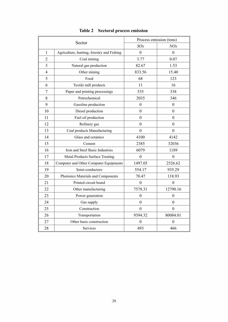
Table 2 Sectoral process emission

Process emission (tons) Sector

SOx NOx 1 Agriculture, hunting, forestry and Fishing 0 0 2 Coal mining 3.77 0.07 3 Natural gas production 82.67 1.53 4 Other mining 833.56 15.40 5 Food 68 123 6 Textile mill products 11 16 7 Paper and printing processings 535 338 8 Petrochemical 2035 346 9 Gasoline production 0 0

10 Diesel production 0 0 11 Fuel oil production 0 0 12 Refinery gas 0 0 13 Coal products Manufacturing 0 0 14 Glass and ceramics 4100 4142 15 Cement 2385 32036 16 Iron and Steel Basic Industries 6079 1189 17 Metal Products Surface Treating 0 0 18 Computer and Other Computer Equipments 1497.05 2526.62 19 Semi-conductors 554.17 935.29 20 Photonics Materials and Components 70.47 118.93 21 Printed circuit board 0 0 22 Other manufacturing 7578.31 12790.16 23 Power generation 0 0 24 Gas supply 0 0 25 Construction 0 0 26 Transportation 9394.32 80084.01 27 Other basic construction 0 0 28 Services 493 466

29

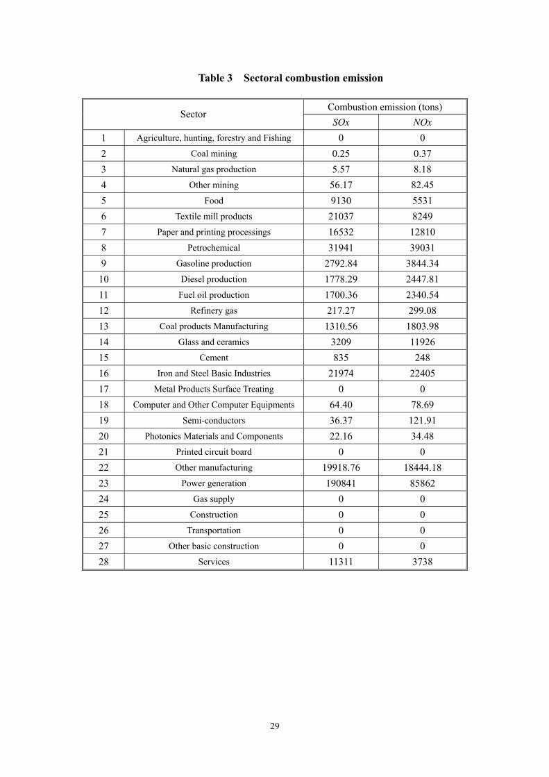
Table 3 Sectoral combustion emission

Combustion emission (tons) Sector

SOx NOx 1 Agriculture, hunting, forestry and Fishing 0 0 2 Coal mining 0.25 0.37 3 Natural gas production 5.57 8.18 4 Other mining 56.17 82.45 5 Food 9130 5531 6 Textile mill products 21037 8249 7 Paper and printing processings 16532 12810 8 Petrochemical 31941 39031 9 Gasoline production 2792.84 3844.34

10 Diesel production 1778.29 2447.81 11 Fuel oil production 1700.36 2340.54 12 Refinery gas 217.27 299.08 13 Coal products Manufacturing 1310.56 1803.98 14 Glass and ceramics 3209 11926 15 Cement 835 248 16 Iron and Steel Basic Industries 21974 22405 17 Metal Products Surface Treating 0 0 18 Computer and Other Computer Equipments 64.40 78.69 19 Semi-conductors 36.37 121.91 20 Photonics Materials and Components 22.16 34.48 21 Printed circuit board 0 0 22 Other manufacturing 19918.76 18444.18 23 Power generation 190841 85862 24 Gas supply 0 0 25 Construction 0 0 26 Transportation 0 0 27 Other basic construction 0 0 28 Services 11311 3738

30

Table 4 Sectoral Process Emission Factor

Emission factor (ton /MNT$) Sector Sectoral Domestic output ( MNT$) V. SOx NOx

Agriculture, hunting, forestry and 466418.79 0.0000 0.0000 Coal mining 267.00 0.0141 0.0003

Natural gas production 5861.99 0.0141 0.0003 Other mining 59105.01 0.0141 0.0003

Food 414220.55 0.0002 0.0003 Textile mill products 376703.28 0.0000 0.0000

Paper and printing processings 248476.02 0.0022 0.0014 Petrochemical 167959.74 0.0121 0.0021

Gasoline production 96896.37 0.0000 0.0000 Diesel production 61696.94 0.0000 0.0000

Fuel oil production 58993.11 0.0000 0.0000 Refinery gas 7538.21 0.0000 0.0000

Coal products Manufacturing 45469.20 0.0000 0.0000 Glass and ceramics 74533.13 0.0550 0.0556

Cement 102291.38 0.0233 0.3132 Iron and Steel Basic Industries 519472.99 0.0117 0.0023

Metal Products Surface Treating 30764.87 0.0000 0.0000 Computer and Other Computer 734025.78 0.0020 0.0034

Semi-conductors 271718.16 0.0020 0.0034 Photonics Materials and Components 34551.43 0.0020 0.0034

Printed circuit board 176933.28 0.0000 0.0000 Other manufacturing 3715758.66 0.0020 0.0034

Power generation 259108.02 0.0000 0.0000 Gas supply 31072.00 0.0000 0.0000

Construction 949183.00 0.0000 0.0000 Transportation 579802.00 0.0162 0.1381

Other basic construction 335370.86 0.0000 0.0000 Services 6135252.21 0.0001 0.0001

Table 5 Transportation Emission factor�ton /MNT$�

SOx SOx NOx NOx

Emission factor of gasoline

Emission factor of diesel

Emission factor of gasoline

Emission factor of diesel

The rest of sectors 0.0213 0.1296 0.3678 1.2500

Natural gas production 0.0000 0.1296 0.0000 1.2500

Gas supply 0.0213 0.0000 0.3678 0.0000

Transportation 0.0000 0.0000 0.0000 0.0000

31

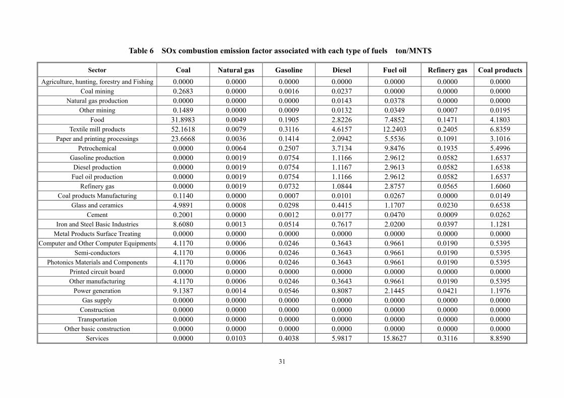
Table 6 SOx combustion emission factor associated with each type of fuels �ton/MNT$�

Sector Coal Natural gas Gasoline Diesel Fuel oil Refinery gas Coal products Agriculture, hunting, forestry and Fishing 0.0000 0.0000 0.0000 0.0000 0.0000 0.0000 0.0000

Coal mining 0.2683 0.0000 0.0016 0.0237 0.0000 0.0000 0.0000 Natural gas production 0.0000 0.0000 0.0000 0.0143 0.0378 0.0000 0.0000

Other mining 0.1489 0.0000 0.0009 0.0132 0.0349 0.0007 0.0195 Food 31.8983 0.0049 0.1905 2.8226 7.4852 0.1471 4.1803

Textile mill products 52.1618 0.0079 0.3116 4.6157 12.2403 0.2405 6.8359 Paper and printing processings 23.6668 0.0036 0.1414 2.0942 5.5536 0.1091 3.1016

Petrochemical 0.0000 0.0064 0.2507 3.7134 9.8476 0.1935 5.4996 Gasoline production 0.0000 0.0019 0.0754 1.1166 2.9612 0.0582 1.6537 Diesel production 0.0000 0.0019 0.0754 1.1167 2.9613 0.0582 1.6538

Fuel oil production 0.0000 0.0019 0.0754 1.1166 2.9612 0.0582 1.6537 Refinery gas 0.0000 0.0019 0.0732 1.0844 2.8757 0.0565 1.6060

Coal products Manufacturing 0.1140 0.0000 0.0007 0.0101 0.0267 0.0000 0.0149 Glass and ceramics 4.9891 0.0008 0.0298 0.4415 1.1707 0.0230 0.6538

Cement 0.2001 0.0000 0.0012 0.0177 0.0470 0.0009 0.0262 Iron and Steel Basic Industries 8.6080 0.0013 0.0514 0.7617 2.0200 0.0397 1.1281

Metal Products Surface Treating 0.0000 0.0000 0.0000 0.0000 0.0000 0.0000 0.0000 Computer and Other Computer Equipments 4.1170 0.0006 0.0246 0.3643 0.9661 0.0190 0.5395

Semi-conductors 4.1170 0.0006 0.0246 0.3643 0.9661 0.0190 0.5395 Photonics Materials and Components 4.1170 0.0006 0.0246 0.3643 0.9661 0.0190 0.5395

Printed circuit board 0.0000 0.0000 0.0000 0.0000 0.0000 0.0000 0.0000 Other manufacturing 4.1170 0.0006 0.0246 0.3643 0.9661 0.0190 0.5395

Power generation 9.1387 0.0014 0.0546 0.8087 2.1445 0.0421 1.1976 Gas supply 0.0000 0.0000 0.0000 0.0000 0.0000 0.0000 0.0000

Construction 0.0000 0.0000 0.0000 0.0000 0.0000 0.0000 0.0000 Transportation 0.0000 0.0000 0.0000 0.0000 0.0000 0.0000 0.0000

Other basic construction 0.0000 0.0000 0.0000 0.0000 0.0000 0.0000 0.0000 Services 0.0000 0.0103 0.4038 5.9817 15.8627 0.3116 8.8590

32

Table 7 NOx combustion emission factor associated with each type of fuels �ton/MNT$�

Sector Coal Natural gas Gasoline Diesel Fuel oil Refinery gas Coal products

Agriculture, hunting, forestry and Fishing 0.0000 0.0000 0.0000 0.0000 0.0000 0.0000 0.0000 Coal mining 0.3947 0.0000 0.0988 0.0107 0.0000 0.0000 0.0000

Natural gas production 0.0000 0.0092 0.0000 0.0009 0.0057 0.0000 0.0000 Other mining 0.1737 0.0504 0.0435 0.0047 0.0309 0.0106 0.0344

Food 21.4777 6.2269 5.3749 0.5800 3.8254 1.3168 4.2566 Textile mill products 25.8305 7.4888 6.4642 0.6975 4.6007 1.5837 5.1192

Paper and printing processings 21.0693 6.1084 5.2727 0.5689 3.7527 1.2917 4.1756 Petrochemical 0.0000 8.1684 7.0508 0.7608 5.0182 1.7274 5.5838

Gasoline production 0.0000 3.8169 3.2947 0.3555 2.3449 0.8072 2.6092 Diesel production 0.0000 3.8170 3.2948 0.3555 2.3450 0.8072 2.6093

Fuel oil production 0.0000 3.8169 3.2947 0.3555 2.3449 0.8072 2.6092 Refinery gas 0.0000 3.7067 3.1996 0.3452 2.2772 0.7839 2.5339

Coal products Manufacturing 0.1556 0.0000 0.0389 0.0042 0.0277 0.0000 0.0308 Glass and ceramics 9.0265 2.6170 2.2589 0.2437 1.6077 0.5534 1.7889

Cement 0.0597 0.0173 0.0149 0.0016 0.0106 0.0037 0.0118 Iron and Steel Basic Industries 6.9269 2.0083 1.7335 0.1870 1.2338 0.4247 1.3728

Metal Products Surface Treating 0.0000 0.0000 0.0000 0.0000 0.0000 0.0000 0.0000 Computer and Other Computer

i3.6558 1.0599 0.9149 0.0987 0.6511 0.2241 0.7245

Semi-conductors 3.6558 1.0599 0.9149 0.0987 0.6511 0.2241 0.7245 Photonics Materials and Components 3.6558 1.0599 0.9149 0.0987 0.6511 0.2241 0.7245

Printed circuit board 0.0000 0.0000 0.0000 0.0000 0.0000 0.0000 0.0000 Other manufacturing 3.6558 1.0599 0.9149 0.0987 0.6511 0.2241 0.7245

Power generation 3.8707 1.1222 0.9687 0.1045 0.6894 0.2373 0.7671 Gas supply 0.0000 0.0000 0.0000 0.0000 0.0000 0.0000 0.0000

Construction 0.0000 0.0000 0.0000 0.0000 0.0000 0.0000 0.0000 Transportation 0.0000 0.0000 0.0000 0.0000 0.0000 0.0000 0.0000

Other basic construction 0.0000 0.0000 0.0000 0.0000 0.0000 0.0000 0.0000 Services 0.0000 0.3437 1.6317 0.1761 1.1613 0.2898 1.2922

33

Table 8 Average Abatement Cost of Air Pollutants for US Industries, 1979~1985 Unit: NT$1997/ton

ISIC Sector PM SOx NOx,CO2 HC 3110 Food 2966.45 17971.14 7899.03 5587.96 3130 Beverages 5381.00 9347.75 411094.24 411094.24 3140 Tobacco 9244.27 5760.42 5760.42 414957.51 3210 Textiles 13659.45 13659.45 47566.62 47566.62 3211 Spinning 9382.25 18454.05 49360.28 6484.79 3220 Apparel 15349.63 2104.11 2104.11 2104.11 3230 Leather 4553.15 13004.07 290780.70 21834.42 3240 Footwear 18626.52 7140.17 34252.10 53740.96 3310 Wood 1621.20 1310.76 1310.76 1310.76 3320 Furniture 1483.22 862.34 862.34 862.34 3410 Paper Products 3000.94 12555.66 16280.96 16280.96 3411 Pulp, Paper 1483.22 5346.50 689.87 689.87 3420 Printing 14625.27 4035.75 10658.51 10589.52 3511 Industrial Chemicals 1586.70 2587.02 10486.04 7347.13 3512 Agricultural Chemicals 4380.68 17902.16 30664.77 11762.30 3513 Resins 2828.47 19385.38 7140.17 4242.71 3520 Chemical Products 7312.63 23490.11 1655.69 5415.49 3522 Drugs 9278.77 36045.77 15556.60 5967.39 3530 Refineries 11313.89 5691.44 2035.12 4173.72 3540 Petroleum, Coal 2035.12 67020.99 2656.00 2656.00 3550 Rubber 7554.09 38184.37 11831.29 11831.29 3560 Plastic 7554.09 83301.94 8105.99 8105.99 3610 Pottery 6381.31 3656.32 130799.58 130799.58 3620 Glass 6415.80 18971.46 11693.32 11693.32 3690 Non-Metal Products 689.87 7347.13 56810.89 57190.32 3710 Iron, Steel 6277.83 18212.60 3966.76 41495.75 3720 Non-Ferrous Metals 11727.81 5243.02 1690.18 22834.74 3810 Metal Products 11831.29 53913.43 15901.53 13762.93 3820 Other Machinery 8761.36 29491.99 17764.18 17764.18

3825 Office, Computing

Machinery 8450.92 8450.92 29802.44 32320.46 3830 Other Electrical Machinery 12866.10 16660.39 53775.46 7416.12 3832 Radio, TV 13590.46 63951.06 31182.18 37804.94 3840 Transport Equipment 21903.41 43668.85 16142.99 34700.52 3841 Shipbuilding 4311.69 28698.64 76886.14 76886.14 3843 Motor Vehicles 12072.75 52533.69 39840.06 84198.78 3850 Professional Goods 41668.22 105067.38 30078.38 47463.14 3900 Other Industries 1310.76 896.83 3794.29 3794.29

34

Table 9 Sectoral unit abatement cost

Sector SOx NOx Sector 1 to 4

(Agriculture, , hunting, forestry and Fishing, Coal mining, Natural gas

production, Other mining)

23552.00 7697.00

Food 17971.14 7899.03 Textile mill products 13659.45 47566.62

Paper and printing processings 7312.63 9209.78 Petrochemical 2587.02 10486.04

Gasoline production 67020.99 2656.00 Diesel production 67020.99 2656.00

Fuel oil production 67020.99 2656.00 Refinery gas 67020.99 2656.00

Coal products Manufacturing 67020.99 2656.00 Glass and ceramics 11313.89 71246.45

Cement 7347.13 56810.89 Iron and Steel Basic Industries 18212.60 3966.76

Metal Products Surface Treating 53913.43 15901.53 Computer and Other Computer

Equipments 8450.92 29802.43

Semi-conductors 105067.38 30078.38 Photonics Materials and Components 105067.38 30078.38

Printed circuit board 105067.38 30078.38 Other manufacturing 33700.21 34197.90

The rest sector (from sector 23 to 28) 23552.00 7697.00

35

Table 10 Emission factors of different types of fuel

Untreated emission factors Coal (103 ton)

Coal products (103 ton)

Gasoline (103 KL)

Diesel (103 KL) Fuel oil (103 KL) LPG (103 KL) Natural gas (106 M3)

SOx 19.5*(1) 19.5*(1) 17.25*(0.05) 17.25*(0.62) 19.25*(0.75) 0.343 0.01 NOx 9.1 9.1 2.8 2.8 7.5 2.24 2.24

Table 11 Energy Consumption and Pollution Emissions in Taiwan, 1997

Untreated Emission �ton� Types of fuel Final Energy

Consumption Transformation

Input

Final Energy Consumption and

Transformation Input SOx NOx

Coal (103 ton) 5,896.828 27,889.483 33,786.311 658,833.06 307,455

Coal products (103 ton) 4,083.031 0.000 4,083.031 79,619 37,156

Gasoline (103 KL) 8,552.043 25.822 8,577.865 7,398 24,018

Diesel (103 KL) 4,902.130 162.440 5,064.570 54,166 14,181

Fuel oil (103 KL) 7,451.519 6,749.344 14,200.863 205,025 106,506

LPG (103 KL) 5,103.400 20.899 5,124.299 1,758 11,478

Natural gas (106 M3) 2,687.385 6,194.407 8,881.792 89 19,895

Total 38,676 41,042 79,719 1,006,888 520,690

36

� 12 Contribution of Energy Combustion on The Intensity of Air Pollution in Taiwan

Average Intensity

Types of Fuel SOx (ppm) Ratio NOx (ppm) Ratio

Coal (103 ton) 0.0039 65.43% 0.0142 59.05%

Coal products (103 ton) 0.0005 7.91% 0.0017 7.14%

Gasoline (103 KL) 4.4E-05 0.73% 0.0011 4.61%

Diesel (103 KL) 0.0003 5.38% 0.0007 2.72%

Fuel oil (103 KL) 0.0012 20.36% 0.0049 20.45%

LPG (103 KL) 1.0E-05 0.17% 0.0005 2.20%

Natural gas (106 M3) 5.3E-07 0.01% 0.0009 3.82%

Total 0.006 100% 0.024 100.00%

37

Table 13 The private health cost associated with SOx pollution from each fuel use

����� SOx �������

���������� �����SOx����

�� SOx ������

���� Population

in 1997 Days in a

year

private health

cost per unit of air pollution emission

The private health cost

associated with SOx pollution from per unit

fuel use

���� 1 �� SOx �������

���� 1 �� SOx �������

a b c = a / b d e f g h = c*d*e*f*g/1000

i = h / emission

factor j = i *1000

Fuel (unit) ppm 103 KL/ 103 ton ppm/103 KL ppm person day

NT$/ person, per day

NT$/ KL NT$/Kg NT$/ton

Coal (103 ton) 0.0039 33786.311 1.162E-07 0.142133 21742815 365 520.1031 68.171 3.496 3495.934

Coal products (103 ton) 0.0005 4083.031 1.162E-07 0.142133 21742815 365 520.1031 68.171 3.496 3495.934

Gasoline (103 KL) 4.4E-05 8577.865 5.140E-09 0.142133 21742815 365 520.1031 3.015 3.496 3495.934

Diesel (103 KL) 0.0003 5064.57 6.373E-08 0.142133 21742815 365 520.1031 37.389 3.496 3495.934

Fuel oil (103 KL) 0.0012 14200.863 8.603E-08 0.142133 21742815 365 520.1031 50.473 3.496 3495.934

LPG (103 KL) 1.0E-05 5124.298528 2.044E-09 0.142133 21742815 365 520.1031 1.199 3.496 3495.934

Natural gas (106 M3) 5.3E-07 8881.792 5.959E-11 0.142133 21742815 365 520.1031 0.035 3.496 3495.934

38

Table 14 The private health cost associated with NOx pollution from each fuel use

����� NOx �������

���������� ����� NOx ��

���� NOx �������

��� Population

in 1997 Days in a year

private health cost per unit of

air pollution emission

The private health cost

associated with NOx pollution from per unit

fuel use

The private health cost of per kilogram

NOx emission

The private health cost of per

ton NOx emission

a b c = a / b d e f g h =

c*d*e*f*g /1000

i = h / emission

factor j = i *1000

Fuel (unit) ppm 103 KL/ 103 ton ppm/103 KL ppm person day

NT$/ person, per

dayNT$/ KL NT$/Kg NT$/ton

Coal (103 ton) 0.0142 33786.311 4.194E-07 0.000903875 21742815 365 520.1031 1.565 0.172 171.964

Coal products (103 ton) 0.0017 4083.031 4.194E-07 0.000903875 21742815 365 520.1031 1.565 0.172 171.964

Gasoline (103 KL) 0.0011 8577.865 1.291E-07 0.000903875 21742815 365 520.1031 0.482 0.172 171.964

Diesel (103 KL) 0.0007 5064.57 1.291E-07 0.000903875 21742815 365 520.1031 0.482 0.172 171.964

Fuel oil (103 KL) 0.0049 14200.863 3.457E-07 0.000903875 21742815 365 520.1031 1.290 0.172 171.964

LPG (103 KL) 0.0005 5124.298528 1.032E-07 0.000903875 21742815 365 520.1031 0.385 0.172 171.964

Natural gas (106 M3) 0.0009 8881.792 1.032E-07 0.000903875 21742815 365 520.1031 0.385 0.172 171.964

39

Table 15 Macroeconomic effects

Baseline result (MNT$)

Scenario 1 (MNT$) % of change Scenario 2

(MNT$) % of change Scenario 3 (MNT$) % of change

Gross Domestic Product 8131152.00 8130613.00 -0.00663 8130071.00 -0.01329 8129959.00 -0.01467

Domestic total output 15627050.27 15625677.62 -0.00878 15624300.59 -0.01760 15624078.80 -0.01901

Exports 4003495.22 4003364.56 -0.00326 4003233.61 -0.00653 4003226.71 -0.00671

Imports 3780185.31 3780375.99 0.00504 3780568.68 0.01014 3780479.91 0.00779

Indirect tax 573274.00 573230.20 -0.00764 573186.20 -0.01532 573187.10 -0.01516

Tariff tax 158030.00 158047.20 0.01088 158064.60 0.02189 158060.80 0.01949

Investment demand 1791300.49 1791511.90 0.01180 1791724.80 0.02369 1791661.40 0.02015

Total labor income 4260962.00 4260498.00 -0.01089 4260031.00 -0.02185 4259894.00 -0.02506

Wage rate 78.21 78.20 -0.01384 78.19 -0.02775 78.19 -0.03257

Total depreciation 771968.00 771992.50 0.00317 772017.20 0.00637 772023.40 0.00718

Capital Income 2568527.00 2568454.00 -0.00284 2568381.00 -0.00568 2568403.00 -0.00483

Household income 6895596.00 6895067.00 -0.00767 6894536.00 -0.01537 6894418.00 -0.01708 Current account

surplus 217225.00 216990.20 -0.10809 216752.10 -0.21770 216844.50 -0.17516

Household savings 1062990.00 1062908.00 -0.00771 1062827.00 -0.01533 1062808.00 -0.01712

Government savings 173568.00 173520.40 -0.02742 173472.70 -0.05491 173468.40 -0.05738 SOx emission-reduced

rate 8 1.00000 0.90056 -9.94377 0.80100 -19.89985 0.80118 -19.88182

NOx emission-reduced rate 1.00000 0.90033 -9.96733 0.80058 -19.94182 0.80069 -19.93124

40

Table 16 Sectoral Effects�% of change� Total air pollution X (Domestic output , MNT$ ) L (Labor, thousand)

Sector Baseline Result Scenario 1 Scenario 2 Scenario 3 Baseline Result Scenario 1 Scenario 2 Scenario 3 Baseline Result Scenario 1 Scenario 2 Scenario 3

1 8963.201** -9.966 -19.940 -19.929 466418.800 -0.0011 -0.0021 -0.0024 878.000 0.00006 0.00009 0.000522 6.073 -10.003 -20.006 -20.011 267.000 -0.0579 -0.1160 -0.1421 0.065 -0.056 -0.113 -0.1393 104.309 -9.995 -19.991 -19.990 5861.990 -0.0529 -0.1060 -0.1260 2.104 -0.063 -0.127 -0.1514 5461.183 -9.977 -19.959 -19.953 59105.010 -0.0172 -0.0344 -0.0414 10.831 -0.021 -0.041 -0.0505 15163.140 -9.961 -19.931 -19.917 414220.600 -0.0090 -0.0180 -0.0193 107.004 -0.005 -0.010 -0.0096 29519.720 -9.967 -19.941 -19.930 376703.300 -0.0182 -0.0364 -0.0425 167.311 0.000 -0.001 0.0017 30518.630 -9.979 -19.962 -19.954 248476.000 -0.0271 -0.0544 -0.0632 133.128 -0.023 -0.047 -0.0548 73431.340 -9.988 -19.978 -19.974 167959.700 -0.0345 -0.0692 -0.0814 19.360 -0.014 -0.029 -0.0309 6815.405 -9.972 -19.949 -19.940 96896.370 -0.0155 -0.0310 -0.0368 6.109 0.012 0.024 0.030

10 4339.577 -9.970 -19.946 -19.937 61696.940 -0.0135 -0.0270 -0.0328 3.890 0.017 0.034 0.04011 4149.401 -9.985 -19.974 -19.971 58993.110 -0.0309 -0.0619 -0.0745 3.719 -0.026 -0.053 -0.06412 530.628 -9.976 -19.957 -19.949 7538.215 -0.0199 -0.0399 -0.0480 0.434 0.001 0.002 0.00213 3130.726 -9.961 -19.931 -19.922 45469.200 -0.0041 -0.0080 -0.0140 1.501 0.087 0.174 0.18514 23488.960 -10.026 -20.045 -20.056 74533.130 -0.0728 -0.1458 -0.1749 36.214 0.113 0.225 0.27015 37005.140 -9.976 -19.957 -19.954 102291.400 -0.0116 -0.0233 -0.0338 49.994 0.264 0.529 0.62616 52513.770 -9.969 -19.946 -19.935 519473.000 -0.0164 -0.0329 -0.0383 91.605 -0.013 -0.027 -0.02917 148.418** -9.975 -19.955 -19.943 30764.870 -0.0105 -0.0209 -0.0199 19.646 -0.016 -0.032 -0.03018 4364.720 -9.958 -19.925 -19.912 734025.800 0.0007 0.0015 0.0020 225.803 0.003 0.007 0.00719 1799.425 -9.962 -19.932 -19.915 271718.200 -0.0025 -0.0050 -0.0009 79.587 0.004 0.008 0.00420 257.757 -9.965 -19.938 -19.924 34551.430 -0.0071 -0.0142 -0.0136 10.575 -0.005 -0.011 -0.02121 164.400** -9.967 -19.942 -19.931 176933.300 -0.0021 -0.0042 -0.0048 53.914 -0.004 -0.008 -0.00922 64005.070 -9.971 -19.948 -19.932 3715759.000 -0.0151 -0.0303 -0.0279 1560.206 -0.015 -0.029 -0.03323 283155.700 -10.044 -20.078 -20.092 259108.000 -0.1023 -0.2049 -0.2429 29.491 0.386 0.775 0.94124 39.565** -9.972 -19.951 -19.942 31072.000 -0.0072 -0.0144 -0.0171 2.394 -0.011 -0.021 -0.02525 3427.786** -9.958 -19.925 -19.916 949183.000 0.0084 0.0170 0.0139 885.000 0.011 0.023 0.01926 89478.340 -9.969 -19.944 -19.934 579802.000 -0.0041 -0.0082 -0.0096 289.167 0.010 0.019 0.02327 1980.864** -9.969 -19.945 -19.934 335370.900 -0.0045 -0.0091 -0.0090 178.949 -0.008 -0.016 -0.01628 28548.110 -9.959 -19.927 -19.913 5802858.000 -0.0022 -0.0044 -0.0049 4007.000 -0.003 -0.006 -0.007

41

Table 16 Sectoral Effects�% of change�-continued M �Imports, MNT$� E �Exports, MNT$� D �Domestic Demand, MNT$�

Sector Baseline Result Scenario 1 Scenario 2 Scenario 3 Baseline Result Scenario 1 Scenario 2 Scenario 3 Baseline Result Scenario 1 Scenario 2 Scenario 3

1 130985.200 -0.018 -0.036 -0.039 39037.870 0.003 0.005 0.006 427380.900 -0.0014 -0.0028 -0.00312 45526.880 -0.038 -0.076 -0.093 8.861 -0.021 -0.041 -0.051 258.139 -0.0592 -0.1186 -0.14523 15720.520 -0.050 -0.100 -0.118 1.108 -0.003 -0.006 -0.008 5860.883 -0.0529 -0.1061 -0.12614 179677.300 -0.015 -0.030 -0.036 1529.572 -0.002 -0.005 -0.006 57575.440 -0.0176 -0.0352 -0.04245 99116.070 -0.014 -0.027 -0.027 78388.080 0.001 0.001 0.001 335832.500 -0.0112 -0.0224 -0.02396 55712.650 -0.001 -0.003 0.005 268537.900 -0.013 -0.025 -0.031 108165.300 -0.0322 -0.0644 -0.07137 76638.230 0.013 0.026 0.036 31969.280 -0.018 -0.036 -0.045 216506.700 -0.0285 -0.0571 -0.06608 156916.700 0.005 0.011 0.019 22820.640 -0.017 -0.034 -0.043 145139.100 -0.0373 -0.0747 -0.08769 10637.940 0.012 0.025 0.031 230.377 -0.012 -0.024 -0.030 96666.000 -0.0155 -0.0310 -0.0368

10 4517.087 0.016 0.032 0.038 7714.316 -0.013 -0.026 -0.031 53982.630 -0.0136 -0.0272 -0.033111 17876.030 -0.021 -0.041 -0.049 9446.575 -0.006 -0.013 -0.016 49546.530 -0.0356 -0.0712 -0.085712 5453.473 0.004 0.009 0.011 5.538 -0.011 -0.021 -0.026 7532.677 -0.0199 -0.0399 -0.048013 921.504 0.102 0.205 0.219 53.164 -0.046 -0.092 -0.101 45416.030 -0.0040 -0.0079 -0.013814 20212.420 0.107 0.215 0.260 23267.000 -0.077 -0.155 -0.187 51266.140 -0.0707 -0.1416 -0.169615 5575.958 0.221 0.443 0.525 2438.898 -0.100 -0.200 -0.240 99852.480 -0.0095 -0.0189 -0.028716 163321.400 0.007 0.015 0.023 73648.730 -0.010 -0.020 -0.025 445824.300 -0.0175 -0.0350 -0.040517 0.000 0.000 0.000 0.000 0.000 0.000 0.000 0.000 30764.870 -0.0105 -0.0209 -0.019918 120242.000 0.000 -0.001 -0.002 579146.300 0.001 0.002 0.002 154879.500 0.0003 0.0006 0.000419 321902.600 -0.001 -0.003 -0.002 253156.900 -0.002 -0.005 -0.001 18561.240 -0.0039 -0.0078 -0.002820 47958.280 0.000 0.000 0.000 20457.060 -0.007 -0.014 -0.014 14094.370 -0.0070 -0.0141 -0.013321 36886.490 -0.005 -0.009 -0.008 143984.700 -0.001 -0.002 -0.003 32948.590 -0.0059 -0.0119 -0.011222 1680818.000 0.016 0.032 0.026 1745139.000 -0.003 -0.006 -0.006 1970620.000 -0.0257 -0.0516 -0.047823 1089.779 0.000 0.001 0.006 567.083 0.000 0.000 0.000 258540.900 -0.1025 -0.2053 -0.243424 121.341 -0.008 -0.015 -0.018 187.182 0.000 0.000 0.000 30884.820 -0.0072 -0.0144 -0.017325 8259.195 0.011 0.022 0.020 3931.920 0.000 0.000 0.000 945251.100 0.0085 0.0171 0.014026 104486.000 -0.006 -0.012 -0.013 243556.400 0.000 0.000 0.000 336245.600 -0.0071 -0.0142 -0.016627 18327.060 -0.013 -0.025 -0.026 63781.270 0.000 0.000 0.000 271589.600 -0.0056 -0.0112 -0.011128 451285.200 -0.008 -0.017 -0.019 390489.500 0.000 0.000 0.000 5412369.000 -0.0024 -0.0047 -0.0053

42

Table 16 Sectoral Effects�% of change�-continued Q (Composite goods, MNT$) INTD�Intermediate goods, MNT$�

Sector Baseline Result Scenario 1 Scenario 2 Scenario 3 Baseline

Result Scenario 1 Scenario 2 Scenario 3

1 564467.600 -0.0054 -0.0107 -0.0119 309369.400 -0.007 -0.015 -0.016 2 46001.390 -0.0380 -0.0760 -0.0930 35712.800 -0.052 -0.105 -0.126 3 22405.920 -0.0508 -0.1017 -0.1198 23240.740 -0.048 -0.097 -0.115 4 241666.300 -0.0156 -0.0312 -0.0374 237752.600 -0.016 -0.032 -0.038 5 447108.400 -0.0118 -0.0236 -0.0247 164612.100 -0.006 -0.012 -0.012 6 166335.800 -0.0214 -0.0429 -0.0447 191772.700 -0.016 -0.033 -0.035 7 295166.900 -0.0174 -0.0350 -0.0387 277260.700 -0.012 -0.025 -0.028 8 303680.700 -0.0151 -0.0302 -0.0321 254861.900 -0.020 -0.040 -0.042 9 122833.300 -0.0096 -0.0192 -0.0223 63118.120 -0.005 -0.009 -0.011

10 58499.710 -0.0113 -0.0226 -0.0276 51035.330 -0.014 -0.029 -0.034 11 68325.870 -0.0315 -0.0631 -0.0757 51838.860 -0.045 -0.091 -0.106 12 13624.760 -0.0091 -0.0182 -0.0216 12621.900 -0.011 -0.021 -0.025 13 46352.240 -0.0019 -0.0036 -0.0091 20310.890 -0.019 -0.039 -0.047 14 72561.470 -0.0184 -0.0369 -0.0436 69746.970 -0.009 -0.017 -0.021 15 106249.800 0.0043 0.0088 0.0045 111288.200 0.005 0.010 0.006 16 614535.000 -0.0106 -0.0213 -0.0232 573410.700 -0.012 -0.024 -0.026 17 30764.870 -0.0105 -0.0209 -0.0199 25967.820 -0.015 -0.029 -0.027 18 278483.600 0.0000 -0.0001 -0.0007 166417.200 -0.003 -0.006 -0.005 19 341778.800 -0.0016 -0.0032 -0.0020 300257.700 -0.003 -0.006 -0.004 20 62165.030 -0.0015 -0.0031 -0.0026 56472.880 -0.003 -0.006 -0.005 21 70641.750 -0.0053 -0.0106 -0.0094 78441.760 -0.004 -0.007 -0.006 22 3749634.000 -0.0059 -0.0119 -0.0128 2127307.000 -0.010 -0.020 -0.020 23 259630.700 -0.1021 -0.2045 -0.2424 233111.800 -0.023 -0.047 -0.053 24 31006.160 -0.0072 -0.0144 -0.0173 11815.330 -0.013 -0.025 -0.030 25 953510.300 0.0085 0.0171 0.0140 195110.500 -0.004 -0.008 -0.009 26 440731.600 -0.0068 -0.0136 -0.0158 202033.000 -0.007 -0.013 -0.015 27 289916.600 -0.0060 -0.0121 -0.0121 230121.700 -0.005 -0.010 -0.011 28 5863692.000 -0.0028 -0.0057 -0.0064 2424718.000 -0.007 -0.013 -0.014

43

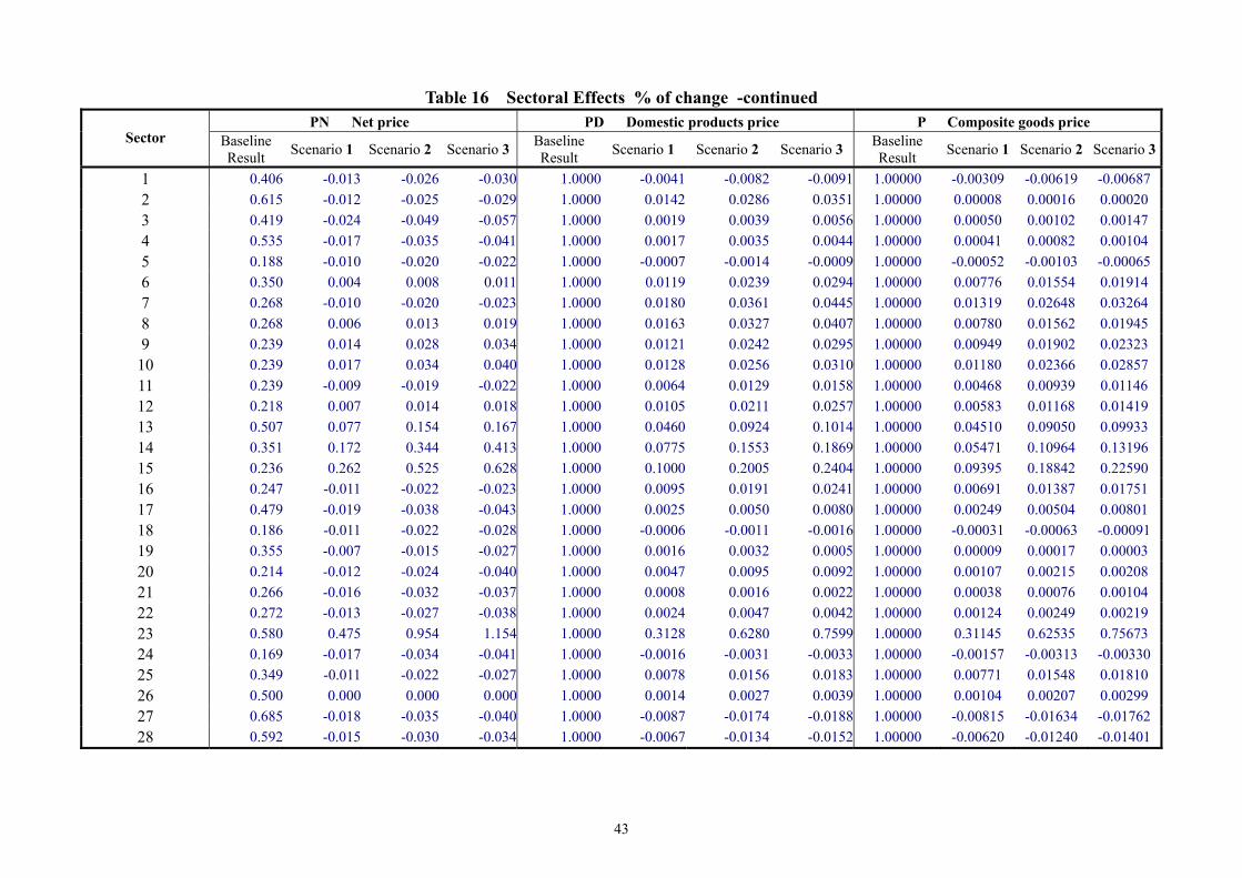
Table 16 Sectoral Effects�% of change�-continued PN �Net price� PD �Domestic products price� P �Composite goods price�

Sector Baseline Result Scenario 1 Scenario 2 Scenario 3 Baseline

Result Scenario 1 Scenario 2 Scenario 3 Baseline Result Scenario 1 Scenario 2 Scenario 3

1 0.406 -0.013 -0.026 -0.030 1.0000 -0.0041 -0.0082 -0.0091 1.00000 -0.00309 -0.00619 -0.00687 2 0.615 -0.012 -0.025 -0.029 1.0000 0.0142 0.0286 0.0351 1.00000 0.00008 0.00016 0.00020 3 0.419 -0.024 -0.049 -0.057 1.0000 0.0019 0.0039 0.0056 1.00000 0.00050 0.00102 0.00147 4 0.535 -0.017 -0.035 -0.041 1.0000 0.0017 0.0035 0.0044 1.00000 0.00041 0.00082 0.00104 5 0.188 -0.010 -0.020 -0.022 1.0000 -0.0007 -0.0014 -0.0009 1.00000 -0.00052 -0.00103 -0.00065 6 0.350 0.004 0.008 0.011 1.0000 0.0119 0.0239 0.0294 1.00000 0.00776 0.01554 0.01914 7 0.268 -0.010 -0.020 -0.023 1.0000 0.0180 0.0361 0.0445 1.00000 0.01319 0.02648 0.03264 8 0.268 0.006 0.013 0.019 1.0000 0.0163 0.0327 0.0407 1.00000 0.00780 0.01562 0.01945 9 0.239 0.014 0.028 0.034 1.0000 0.0121 0.0242 0.0295 1.00000 0.00949 0.01902 0.02323

10 0.239 0.017 0.034 0.040 1.0000 0.0128 0.0256 0.0310 1.00000 0.01180 0.02366 0.02857 11 0.239 -0.009 -0.019 -0.022 1.0000 0.0064 0.0129 0.0158 1.00000 0.00468 0.00939 0.01146 12 0.218 0.007 0.014 0.018 1.0000 0.0105 0.0211 0.0257 1.00000 0.00583 0.01168 0.01419 13 0.507 0.077 0.154 0.167 1.0000 0.0460 0.0924 0.1014 1.00000 0.04510 0.09050 0.09933 14 0.351 0.172 0.344 0.413 1.0000 0.0775 0.1553 0.1869 1.00000 0.05471 0.10964 0.13196 15 0.236 0.262 0.525 0.628 1.0000 0.1000 0.2005 0.2404 1.00000 0.09395 0.18842 0.22590 16 0.247 -0.011 -0.022 -0.023 1.0000 0.0095 0.0191 0.0241 1.00000 0.00691 0.01387 0.01751 17 0.479 -0.019 -0.038 -0.043 1.0000 0.0025 0.0050 0.0080 1.00000 0.00249 0.00504 0.00801 18 0.186 -0.011 -0.022 -0.028 1.0000 -0.0006 -0.0011 -0.0016 1.00000 -0.00031 -0.00063 -0.00091 19 0.355 -0.007 -0.015 -0.027 1.0000 0.0016 0.0032 0.0005 1.00000 0.00009 0.00017 0.00003 20 0.214 -0.012 -0.024 -0.040 1.0000 0.0047 0.0095 0.0092 1.00000 0.00107 0.00215 0.00208 21 0.266 -0.016 -0.032 -0.037 1.0000 0.0008 0.0016 0.0022 1.00000 0.00038 0.00076 0.00104 22 0.272 -0.013 -0.027 -0.038 1.0000 0.0024 0.0047 0.0042 1.00000 0.00124 0.00249 0.00219 23 0.580 0.475 0.954 1.154 1.0000 0.3128 0.6280 0.7599 1.00000 0.31145 0.62535 0.75673 24 0.169 -0.017 -0.034 -0.041 1.0000 -0.0016 -0.0031 -0.0033 1.00000 -0.00157 -0.00313 -0.00330 25 0.349 -0.011 -0.022 -0.027 1.0000 0.0078 0.0156 0.0183 1.00000 0.00771 0.01548 0.01810 26 0.500 0.000 0.000 0.000 1.0000 0.0014 0.0027 0.0039 1.00000 0.00104 0.00207 0.00299 27 0.685 -0.018 -0.035 -0.040 1.0000 -0.0087 -0.0174 -0.0188 1.00000 -0.00815 -0.01634 -0.01762 28 0.592 -0.015 -0.030 -0.034 1.0000 -0.0067 -0.0134 -0.0152 1.00000 -0.00620 -0.01240 -0.01401

44

Table 17 Green Domestic Product

Baseline result(MNT$)

Scenario 1 (MNT$) % of change Scenario 2

(MNT$) % of change Scenario 3 (MNT$) % of change

Gross Domestic Product 8131152.00 8130613.00 -0.006629 8130071.00 -0.013295 8129959.00 -0.014672

SOx maintenance cost 8079.73 7271.65 -10.001278 6463.60 -20.002271 7457.22 -7.704510

NOx maintenance cost 6263.47 5637.20 -9.998754 5010.92 -19.997782 5136.61 -17.990931

Total maintenance cost 14343.20 12908.85 -10.000209 11474.51 -20.000349 12593.84 -12.196442

SOx damage cost 23916.24 21524.62 -9.999983 19132.99 -20.000008 19132.99 -20.000008

NOx damage cost 1251.41 1126.27 -10.000000 1001.13 -20.000000 1001.13 -20.000000

Total damage cost 25167.65 22650.88 -10.000020 20134.12 -20.000000 20134.12 -20.000000

SEEA GREEN GDP 8116809.00 8117704.00 0.011027 8118597.00 0.022028 8117366.00 0.006862

Revised GREEN GDP 8105984.00 8107962.00 0.024402 8109937.00 0.048766 8109825.00 0.047385

Total Depreciation 771968.00 771992.50 0.003174 772017.20 0.006373 772023.40 0.007176

SEEA GREEN NDP 7344841.00 7345711.00 0.011845 7346580.00 0.023676 7345342.00 0.006821

ENRAP GREEN NDP 7334016.00 7335969.00 0.026629 7337920.00 0.053231 7337802.00 0.051622

SOx emission-reduced rate from baseline level 1.00 0.90 -10.00 0.80 -20.00 0.80 -20.00

NOx emission-reduced rate from baseline level 1.00 0.90 -10.00 0.80 -20.00 0.80 -20.00

45