ilable at ScienceDirect

Electoral Studies 30 (2011) 136–147

Contents lists ava

Electoral Studies

journal homepage: www.elsevier .com/locate/e lectstud

Analyzing partisanship in Central Mexico: A geographical approach

Manuel Suárez a,*, Irina Alberro b,1

a Instituto de Geografía, Universidad Nacional Autónoma de México, Circuito Exterior s/n, Ciudad Universitaria, Mexico DF 04510, MexicobCentro de Estudios Internacionales, El Colegio de México, Camino al Ajusco 20, Col. Pedregal de Sta. Teresa, México DF 10740, Mexico

a r t i c l e i n f o

Article history:Received 23 March 2010Received in revised form 10 November 2010Accepted 16 November 2010

Keywords:ElectionsPartisanshipSocioeconomicMexico

* Corresponding author. Tel.: þ52 55 56224333.E-mail addresses: msuarez@igg.unam.mx (M. Suá

mx (I. Alberro).1 Tel.: þ52 55 54493011; fax: þ52 55 56450464.

0261-3794/$ – see front matter � 2010 Elsevier Ltddoi:10.1016/j.electstud.2010.11.014

a b s t r a c t

The article explores the relevance of socioeconomic variables on partisanship in CentralMexico for the 2006 presidential election. We perform an exploratory canonical correla-tion analysis, a predictive binomial logit analysis and a further confirmatory set of OLSregression analyses. The analyses are based on a data set that uses electoral results as wellas census information, constructed as 1.6 km (one mile) radii GIS neighborhoods, whichallow for the integration of electoral and census geographies. The results suggest thatincome and education do not always influence party preferences in the same direction. Inparticular in the case of the vote for the left leaning party, these two variables havecontradicting effects.

� 2010 Elsevier Ltd. All rights reserved.

In the past years, journalists, pundits and researchersamong others, have argued that in electoral terms, Mexicocan be clearly divided according to socioeconomic status. Inparticular, in the 2006 election, many arguments suggestthat the North of the countrydwhich tends to be wealthierthan the Southdvoted for the right leaning party PartidoAcción Nacional (PAN) while the impoverished South wasmore prone to support the leftist Partido de la RevoluciónDemócratica (PRD).

Historically, Mexico was ruled by a unique and verypowerful party, the Partido Revolucionario Institucional(PRI), who retained power for over seven decades. Theconstituency of this party was very heterogeneous in socio-economic as well as geographical terms. Voters from thepoorest strata as well as very wealthy individuals tended tofavor the PRI throughout the country. Since the presidentialelection of 2000when the PRI lost the presidency to the PAN,both geographical aswell as socieconomic cleavages becameapparent. This recent phenomenon requires in depth anal-ysis. As Moreno mentions, “[D]uring the decade of thenineties, the Mexican electorate showed clear signs of being

rez), ialberro@colmex.

. All rights reserved.

divided in two political camps. One is older, with less years ofeducation, lives principally in ruralMexico, althoughyou canalso find him in the cities, has authoritarian tendencies andshares fundamental values [.] [T]he other one is younger,more educated, predominantly urban and has democratic,pro-liberal values” (Moreno, 2003. p. 12).

The generalized premise states that voters living in lessdeveloped areas are more likely to be attracted by the leftand its willingness to favor the situation of the less privi-leged groups. Whilst, the more developed north, with itsindustries, supports the PAN, who is able to provide a moreattractive economic environment for business and is lessconcerned with redistributing income towards the poor.For instance, in 2006, the campaign slogan used by thePRD’s candidate, Manuel López Obrador, “Por el bien detodos, primero los pobres” (For everyone’s well being, firstthe poor) clearly shows the focus of the electoral quarrel.

The purpose of this article is to analyze the relationshipbetween socioeconomic statuses and partisanship inCentral Mexico for the 2006 presidential election. On theone hand, we analyze the electoral results according to thetraditional political science vision of partisanship. Onthe other hand we simultaneously use a spatial frameworkto analyze the socioeconomic cleavages of partisanship,which translates into a canonical correlation analysis (CCA).The model allows observing the common variation and

M. Suárez, I. Alberro / Electoral Studies 30 (2011) 136–147 137

specific relevance of aggregated socioeconomic variables inthe decision to support each party (and failing to supportothers simultaneously) in what we have called electoraldimensions. We complement this analysis with a logisticregression, as it may well be a more intuitive (thoughsimpler) analysis that helps explain the results of the CCA.

We use the Central Mexico Region as our study areabecause of its several geographic advantages. (1) It is thedensest region in the country with one-third of the coun-try’s population; (2) it is an integrated region in socioeco-nomic terms, and (3) the six states that comprise the regionhave distinct party traditions as shown in Table 1.

For instance, there are states where the partisan pref-erence seems to fluctuate when electing different levels ofgovernment or between presidential elections. The state ofMexico shows an interesting pattern in this sense, wherethe PAN won in the 2000 electionwhile the leftist coalitionwon in 2006, but the governorship has been in the hands ofthe PRI without party alternation.

We also found it necessary to limit our analysis toa region because of the impossibility of using our meth-odology in a countrywide analysis. Due to spatialmismatches between electoral and census data, and theneed of using the smallest possible levels of aggregation,we use 1.6 km2 (1 mile) GIS generated neighborhoods thatallow the integration of electoral and socioeconomic data.Using this level of aggregation, a countrywide analysiswould be a daunting task.

Although our approach requires certain level of dataaggregation, it offers certain advantages when comparedwith both pre-electoral and exit polls. Mainly, it allowscombining census data (the richest source of socioeco-nomic information) with electoral results. While pre-elec-toral polls may have a great deal of socioeconomicvariables, we would be forced to analyze voting intention,not real vote. In the case of exit polls, they simply do nothave the extensive socioeconomic information such as theone we present in the analyses.

The traditional socioeconomic approach to explainvoting shows that in developed democracies, variables suchas income and education determine turnout and in somecases influence partisanship (Verba and Nie, 1972).According to the general consensus in the literature,education and income are both positively related to polit-ical participation (Verba and Nie, 1972; Almond and Verba,1963; Barnes and Kaase, 1979; and Milbrath, 1965).

In the case of the Mexican elections, Moreno finds thathigher levels of education tend to explain more support forthe PAN while lower levels of education tend to translateinto more support for the PRI. The variable does not seemparticularly relevant, according to his analysis, in the case

Table 1Central Mexico: presidential vote (2000–2006) and current governorship.

State Vote 2000 Vote 2006 Governor

Distrito Federal PAN PRD-PT-Convergencia PRDHidalgo PRI PRD-PT-Convergencia PRIMéxico PAN PRD-PT-Convergencia PRIMorelos PAN PRD-PT-Convergencia PANPuebla PAN PAN PRITlaxcala PRI PRD-PT-Convergencia PAN-PT

of the PRD. Similarly income also plays an important role inthe party identification of the Mexican voter. Individualswith lower levels of income tend to identify more with thePRI and the PRD while those who have higher levels ofincome tend to votemore often for the PAN. As it appears inthe Moreno study, education and incomemove in the samedirection when it comes to explain the likelihood of sup-porting one of the major three parties (Moreno, 2003).

Thus, although it is clear (and intuitive) that these twovariables should have a common variation effect on thedirection of votes, we find that in our study case, this in factis not true, and that the partial effects of income andeducation on the direction of votes actually vary betweenpolitical parties.

The rest of the paper is divided into four sections. First,wesummarize the relevant literature that helps frameour study.For this purpose, we review the work on socioeconomicstatus and partisanship from a comparative perspecti-vedmainly the cases of the United States and Mexicodanddiscuss some of the studies that have used a geographicalapproach in the analysis of the electorate in Mexico. In thesecond section we present our study area and providea summary of the socioeconomic characteristics of voters aswell as the electoral outcome. We then present our meth-odology in a third section. Finally, a fourth section shows ourresults, which we discuss in a fifth and concluding section.

1. Socioeconomic status and partisanship

1.1. The U.S. case

Scholars have long analyzed the relationship betweensocioeconomic status (SES) and turnout. Nonetheless, thereare different opinions regarding the specific role ofdifferent components of SES. It appears unclear whethereducation or income is a stronger predictor of electoralparticipation. Despite the fact that these different compo-nents of SES are highly correlated, there have been studiesthat isolate the specific effect of education and income. Forinstance, some authors argue that the level of educationhas no consistent impact on voting (Milbrath and Goel,1977). Other studies show that education was less impor-tant than income in order to understand voter turnout(Bennett and Klecka, 1970; Verba et al., 1978). Finally, somescholars find that the demographic variable that is moststrongly related to turnout is education (Campbell et al.,1960; Milbrath, 1965; Barber, 1969). Overall, all authorsargue that these two variables tend to have a similar effectin promoting a higher turnout. More recently, studies havefocused on analyzing the effect of these variables onpartisanship rather than just turnout. In this section, wewill briefly summarize and discuss the relevant literaturefor the cases of the US and Mexico.

In the United States there has been much debateregarding the socioeconomic cleavages of partisanship, inparticular the fact that blue statesdwhich are on averagericherdsupport Democrats while the red states, in theirmajority, vote Republican (Gelman et al. 2008; Frank,2004). In this section we discuss two of the most essen-tial variables related to socioeconomic statusdincome and

M. Suárez, I. Alberro / Electoral Studies 30 (2011) 136–147138

educationdand their impact on partisanship in general andmidterm elections in the US since 1980.

It is worth noticing that in the 1984 and 1988elections, turnout for the Republicans increased sig-nificantlydespecially forReagan’s re-electiondandalthoughwealthier countieswere stillmore likely to support this party,less affluent counties started voting for the Republican Party.During Clinton’s first election, it appears that income becameless relevant to define partisanship given that income differ-ences between counties became less significant to under-stand party preferences. The 1996 election followed a similarpattern than the 1992 one but, for the first time since 1980,the richest counties decreased their support for the Repub-lican Party. Interestingly by 2000, the relationship betweenincome and support for the Republican Party adopted aninverse U-shape. The poorest counties and the richest oneswere the less likely to support Bush,while countieswith closeto average income overwhelmingly voted Republican. Thesame pattern can be observed in 2004 (Alberro, 2007).

The complexity in the relationship between income andpartisanship is well summarized by Gelman et al.:

In poor states such as Mississippi, richer people aremuch more likely than poor people to vote Republican,whereas in rich states such as Connecticut, there is verylittle difference in vote choice between the rich and thepoor. This trend has gradually developed since the early1990s and has reached full flower in the elections of2000 and beyond. As a result, richer states now tend tofavor the Democratic candidate, yet in the nation asa whole richer people remain more likely than poorerpeople to vote Republican (Gelman et al., 2010).

Overall, it is clear that the Republican Party’s constituencychanged overtime significantly. From 1980 to 1992, richercounties were more prone to vote for Republican candidates.Nonetheless, when looking at the past two presidentialelections, it would be safe to conclude that Republicansobtained their votes mostly from average income countieswhile losing votes from the richest ones.When looking at theresults for the Democratic Party, it is also interesting to notethat incomewasconsistentlynegatively related to support forthis party in the 1980, 1984 and 1988 presidential elections.In those three cases, a marginal increase in the per-capitaincome of the counties immediately implied a reduction insupport for Democrats. Nonetheless, since 1992 this patternstarted to change such that the richest counties startedcastingmore votes for theDemocratic Party. In the next threeelections �1996, 2000 and 2004– the relationship betweenincome and support for the Democrats became decisivelyU-shaped such that thepoorest counties aswell as the richestones were the ones voting for Democrats in the electionswhile middle income counties were much less prone tosupport this party. Not surprisingly, the examination ofDemocratic support is almost a perfect inverse reflection ofpatterns of support for the Republicans throughout the yearsexcept for the fact that it helps us identify more clearly theshifts that started taking place in 1992 and that made richercounties more favorable to Democrats (Alberro, 2007).

Education has usually been negatively related tosupport for the Democratic Party. From 1980 to 1992,a marginal increase in the percentage of college educated

voters in a county lead to a decrease in support for theDemocrats although the percentage of votes obtained forthis party in the most educated counties tended to increaseslightly. In 1996, the tendency started to change andbecame more U-shaped such that most Democraticsupporters came from the least educated counties and themost educated ones, while counties with close to averageeducation were less likely to support the Democratic Party.This tendency became more and more acute in the 2000and 2004 elections. For instance, the difference in Demo-cratic support in 2004 between counties with averageeducation and the most educated ones was close to 25%.This relationship can also be seen when looking at thecorrelation between Republican votes and education. Themost educated counties have become increasingly lessprone to cast votes in favor of Republican candidates since2000. It should be noted, however, that education andincome tend to be highly correlated variables, thus thesetrends are not surprising (Alberro, 2007).

The literature on American elections provides animportant analytical framework to analyze other electionsin other democracies. The studies cited above show that therelationship between education, income and partisanshipare dynamic across different elections. Income and educa-tion do not always have the same effect on party prefer-ences. Following this academic tradition, in this paper weanalyze the role of income and education on partisanship inMexico, while controlling for a set of other socioeconomicvariables specifically geographical ones. These types ofstudies are rare in Mexico but they have acquired a recentpopularity in American politics as mentioned above.

1.2. The Mexican case

In his very influential study, Barry Ames (1970) foundthat in Mexico, an increase in turnout was positively linkedto the Partido Revolucionario Institutional vote and thatwhenever opposition parties’ presence was strong, elec-toral participation tended to diminish. Surprisingly, Amesalso found that contrary to expectations and to thepredictions of the comparative literature on electoralbehavior, turnout was especially high in poorer and lessurbanized areas. Gónzalez Casanova (1965) also arguedthat poor constituencies were more prone to vote for thePRI, and that those rural impoverished areas with lowlevels of education and precarious public services were thestronghold of that party.

Nonetheless, since the 1970s, the PRI began to lose itstraditional grip on social organizations losing then itscapacity to mobilize voters. Due to the economic crisis ofthe 1980s and the transformation of the previously inter-ventionist state model, the PRI had to reduce the direct andindirect spending that customarily lubricated the votingmachine and mobilized people throughout the country.Despite these significant transformations, the PRI remainedthe party capable of reaching the poorest groups. In 1988,the PRI had for the first time in modern Mexico, a seriouscontender for the presidency by a former member of theparty, Cuauhtémoc Cárdenas.

Poorer municipalities have remained the PRI’s strong-hold up until the last election in 2006, but the party’s

1.02.0

3.04.0

5.06.0

Marginality Index

setoVfonoitroporP

1 2 3 4 5 6 7 8 9 10

PANPRIPRD

Fig. 1. Proportion of votes per party and municipal marginality index,national presidential election, 1994. Source: Authors calculations with 1994election data and CONAPO 2005a marginality data.

1.02.0

3.04.0

5.06.0

Marginality Index

Prop

ortio

n of

Vot

es

PANPRIPRD

1 2 3 4 5 6 7 8 9 10

Fig. 2. Proportion of votes per party and municipal marginality index,national presidential election, 2000. Source: Authors calculations with 2000election data and CONAPO 2005a marginality data.

02.052.0

03.053.0

04.054.0

setoVfonoitroporP

PANPRIPRD

M. Suárez, I. Alberro / Electoral Studies 30 (2011) 136–147 139

dominance has gradually fallen, giving way to the PAN andPRD strengthening. Electoral data for the 1994, 2000 and2006 presidential elections show that poor constituenciesare still strong supporters of the PRI, however the electoralstrength of this party has been diminishing considerably,especially in municipalities with higher levels of welfare,where urban areas are located.

Similarly towhathappens in the studyof other countries,there is some debate regarding which socioeconomic vari-able tends to be determinant when analyzing partisanship.Education, for instance, has been identified by an importantnumber of researchers as a defining variable for supportingthe PAN. Accordingly, individuals with higher levels ofeducation aswell aswhole segments of the populationwithhigher levels of education aremore likely to support thePAN(Molinar and Weldon, 1990; Klesner, 1993,1998, Vilalta,2006). Income, on the other hand, is also an importantdeterminant of partisanship. In particular several authorshave proven that higher income voters are more likely tofavor the PAN and communities with high levels of incomeare less prone to support the PRI or the PRD.

Opposite to the studies above mentioned, Ortega (2008)concluded that different sociodemographic variables hel-ped understand the vote in favor of the PRD in the 2000presidential election in México, of which education waskey; and that an increase in the years of education had ledto an increase in the support for the party.

Figs. 1–3 show voting proportions for PRI, PAN and PRDfor the 1994, 2000, and 2006 elections, respectively, grou-ped into deciles of a municipal marginalization index(CONAPO, 2005a,b)2. Support for the PRI is high in

2 The marginality index is published by the National PopulationCouncil (CONAPO). It is a commonly used index that reflects povertylevels. It is constructed with a principal components analysis thatincludes income, education, level of urbanization and housingcharacteristics.

municipalities with a higher degree of marginality andlower in municipalities with low marginality indices. It isclear that although in general, support for PRI has dimin-ished; wealthier municipalities tend to show more signif-icant changes in their preferences for other parties,especially for the PAN. This maywell be an effect of changesin electoral participation. According to Klesner and Lawson(2001), nowadays, turnout patterns in Mexico are quitesimilar to those found in established democracies whereelectoral competition is strong. According to the authors,“[.] Mexico’s more affluent and politically engaged citi-zens are nowmore likely to participate than the poorer, less

51.0

Marginality Index

1 2 3 4 5 6 7 8 9 10

Fig. 3. Proportion of votes per party and municipal marginality index,national presidential election, 2006. Source: Authors calculations with 2006election data and CONAPO 2005b marginality data.

M. Suárez, I. Alberro / Electoral Studies 30 (2011) 136–147140

informed, and rural voters who for decades dutifullydelivered their votes to the PRI” (Klesner and Lawson, 2001,p. 19).

According to these authors, the drastic change inturnout took place in the decade of the 1990s when thePRI’s strength became compromised and voters who werepreviously co-opted by the PRI’s machinery became moreautonomous and felt less bound to support the ruling party.The authors conclude that: “[A]s Mexico urbanized and itscitizenry became better educated, the foundations of thePRI’s electoral machine began to crumble. Previouslycaptured PRI supporters were now freer to abstain, andpotential opposition voters could expect that their voteswould be counted honestly. As a result, patterns of electoralparticipation in Mexico began to change.” (Klesner andLawson, 2001, p.21).

In regards to the PAN, it is clear that at the municipallevel, this party has a strong support among richerconstituencies. Indeed, municipalities with high welfareindexes show higher support for the PAN, which also grewin the 1994–2006 period. It is worth noticing that while thePRI and PAN lines cross at the third decile of themarginalityindex in 2000, by 2006 they cross close to the median. Also,that by 2006 both PRI’s and PAN’s voting proportionsgradients as a function of marginality became steeper, andoverall have a clearer pattern.

Instead, in 1994 the PRD’s gradient of voting propor-tions was parallel to the PRI. By 2000, although it still fol-lowed a similar trend, the gradient became a little flatterand by 2006 there seems to be no clear pattern of support.Interestingly enough, for the 2006 election, the welfarelevels of the municipalities are simply not a good predictorof support for this party. This apparent lack of association isthe main focus of our analysis.

1.3. Space and partisanship

In a study using panel data for the 2006 election, Law-son mentions that the role of socioeconomic variables waspredictable, but the most salient predictor of partisanshipwas geographical area (Lawson, 2006). According to theauthor,

[A]lthough indicators of social statusdsuch as livingstandards, education, skin color, and occupa-tiondinfluence voting behavior at the margin, forordinary Mexicans, region is a far more importantpredictor of their partisan preferences.3 Consider, forinstance, the “classic” PRD voter in May 2006: a brown-skinned, low-incomemanwith amodest educationwhonever attends church. A person with this demographicprofile living in the north of the country had a 20%

3 Results are based on simulations from a multinomial logit model ofvote choice, in which the dependent variable took on one of four values(Calderón, López Obrador, Madrazo, or none/undecided). Independentvariables included: age, gender, living standards (as measured by anindex of material possessions, education, church attendance, region,political engagement, skin color, and urban or rural residence). Data aretaken from the Mexico 2006 Panel Study, Wave 2. For full results, seeLawson 2006, available at:http://web.mit.edu/polisci/research/mexico06/Pres.htm.

chance of favoring López Obradordfar lower than hisprobability of favoring Calderón. If his home was in thecenter of the country, however, his probability of sup-porting López Obrador rose to 34%. If he lived in thesouth, it was 44%, and if he resided in the Mexico Citymetropolitan area, it was 72%(Lawson, 2006, p. 9)

Similarly, Moreno suggests that class does not seem topredict partisanship. Moreover, a vast majority of Mexicansdo not vote based on the policy platform proposed byparties (Moreno, 2007). When studying the regionalcomponent of the vote, Cortina et al. (2010) show thatincome matters more in poor states than in rich ones indefining partisanship. In this paper we offer an alternativeapproach to study the role of key socioeconomic variablesto understand partisanship by using a canonical modelwhose basic advantage is to allow the construction ofa model with multiple variables in both sides of the equa-tion. The basic underlying principle is then to maximizethe canonical correlation between the two sides of theequations.

2. Study area

The Central Mexico Region (CMR) (Fig. 4) is an87,360 km2 area with a population of 34.3 million, close toone-third of the population in the country in 2005. It is thenation’s densest region, with only 4.7 percent of thecountry’s area. More than two thirds of its populationreside in nine metropolitan areas, including Mexico Citywith 19 million inhabitants. The region is comprised of sixstates: Hidalgo, México, Morelos, Tlaxcala, Puebla, andDistrito Federal (DF), the nation’s capital.

In the 2006 presidential election the registered voters inthe region represented 23.3 million and turnout was over62% of the registered voters. Overall, the voting results(valid votes) in the region were as follows: 31.3 percent forthe PAN, 47.0 percent for the PRD, 16.3 percent for the PRIand 4.5 percent for other parties (Table 2). Therewas awidemargin in favor of the PRD when comparing this region tothe rest of the country. Instead, support for both the PRI andthe PAN was largely underrepresented in this region whencompared to the national results which signals that geog-raphy matters when it comes to partisanship.

When comparing the region’s electoral results, it is clearthat the PRD’s national stronghold is the country’s capi-taldMexico City. The support for the PAN is more homo-genously distributed across states in the central regionwhile the PRI is weak in the DF and strong in Hidalgo andTlaxcala (the two poorest states in the region). As Fig. 4shows, support for the PRD is at its highest level inMexico City. The second and third largest cities, Puebla (2.2million) and Toluca (1.2million), showed higher support forthe PAN near the central cities and support for the PRD andthe PRI in their peripheries. This spatial pattern is impor-tant becausedcontrary to what we observe in the UnitedStates and Europedlow income housing tends to locate inthe periphery and not in the heart of the cities. Most of thesmaller cities have no clear winning party pattern judgingfrom our map.

Fig. 4. Central Mexico Region: electoral results per electoral section, 2006.

M. Suárez, I. Alberro / Electoral Studies 30 (2011) 136–147 141

Fig. 5 shows voting proportions for each of the threeparties according to the samemarginality index used in theprevious section. Contrary to the national results, in thecase of central Mexico, we can identify a voting pattern forthe PRD such that support increases in municipalities withlow levels of marginality. The vote for the PAN also

Table 2National and regional electoral results, 2006.

PAN PRI PRD Other

National 36.9 22.7 35.9 3.8Central Mexico 31.4 16.3 47.1 4.5Voting Proportions relative to the regionDistrito Federal 0.9 0.5 1.3 0.9Hidalgo 0.9 1.6 0.9 1México 1 1.1 0.9 1.1Morelos 1 1 1 1.2Tlaxcala 1.2 1.5 0.7 0.8Puebla 1.1 0.9 0.9 0.8

reflects a change in its tendency given that the partyobtained a higher level of votes in municipalities with highmarginality in the central region when compared to therest of the country although the tendency is less obvious.On the other hand, the PRI does show the same pattern asin the country as a whole, with increasing proportions ofvotes as the marginality index increases. These, however,are based on municipal figures.

A smaller scale of analysis: 1.6 Km2 (1 mile) neighbor-hoods (See section 3.1), depicts a more detailed votingmap.Table 3 shows mean values for selected socioeconomicvariables that we use in our analyses of the followingsections. Mean income was at its highest in neighborhoodswhere the PAN won and lowest where the PRI waspreferred. The PRD vote reflects an intermediate incomelevel. The same is true for education, access to healthcare,and percentage of Catholic population; although the gapsobserved in these variables between PAN and PRD arelower than the existent gap between these two parties and

2 4 6 8 10

1.02.0

3.04.0

5.0

Marginality Index

setovfonoitroporP

PANPRDPRI

Fig. 5. Central Mexico Region: proportion of votes per party and municipalmarginality index, presidential election, 2006. Source: Authors calculationswith 2006 election data and CONAPO 2005b marginality data.

M. Suárez, I. Alberro / Electoral Studies 30 (2011) 136–147142

the PRI. In general terms, the PRI voters tend to live in moreprecarious conditions at least in this region of the country.The percent of self-employed workers as well as the meannumber of occupants per dwelling unit seem to be higher inPRI winning areas, and lowest in PAN winning areas.

It is also worth noticing that while the difference inincome between places where the PANwins and where thePRD wins is 28 percent, the difference in education is only12 percent. Likewise, the quotient between education andincome is lower for places where the PAN wins (2.5) thanfor places where the PRD or PRI (3) win.

In the case of age, the PRD seems to have less support inplaces with higher percentages of elderly population incontrast to the PRI that is popular among this age group.Finally, the PRI has the highest numbers of home ownerswhile the PAN has the lowest one. This is possibly a result ofa PRI strategy that allowed during years (low-income)informal settlements to develop in the periphery of citieson state-owned land (Cruz Rodriguez, 2001). Votes for the

Table 3Socioeconomic characteristics of GIS neighborhoods per winning party inthe 2006 election.

Variable Winning Party

PAN PRD PRI

Mean income (minimum wages) 3.6 2.8 1.5Mean school years 9.3 8.3 4.5% Pop. 18–25 years old 13.6 13.6 11.7% Pop. 65 þ years old 6.0 4.6 6.2% Population with healthcare 50.0 48.1 12.4% Catholic population 80.0 79.0 75.6% Population with no religion 2.1 2.2 1.2% Self-employed 18.9 20.4 21.1% Female headed HH 25.6 23.0 21.1Mean occupants per DU 3.9 4.2 4.9% Home owners 68.6 70.9 82.1

Source: authors’ calculations electoral and population census data.

PRI were exchanged for the promise of urban services andland tenure (Eckstein, 1977).

3. Methodology

In order to see how partisanship is associated withsocioeconomic status we perform one exploratory canon-ical correlation analysis, one predictive binomial logitanalysis, a further confirmatory set of OLS regressionanalyses product of our findings of the first two as well asdescriptive graphs that help illustrate our findings. We firstdescribe our data, and then give details about the statisticalmethods used.

3.1. Data sources and data set construction

Data sources used in the analysis are the 2000 pop-ulation census tract level data and the 2006 presidentialelection results at the section level. Tract level data is thelowest aggregation level at which census results are pub-lished inMexico. Although electoral results are available forindividual voting booths, our methodology requires similaraggregation spatial units for both socioeconomic andvoting characteristics. However, there are both geometricand size differences between census tracts and electoralsections. On the one hand, both become larger as pop-ulation densities decrease with distance to city centers. Onthe other hand, the spatial match between sections andtracts is far from being perfect. A section may in some casesbe contained inside one tract, although the opposite is alsoplausible. In most cases, both sections and tracts overlapwith each other, making direct comparisons impossible.

To overcome this difficulty, we used circular areas of1.6 km radio (1 mile) that are calculated as GIS neighbor-hoods, otherwise known as a moving window. To do so, wecalculated densities per hectare for each of our variables ineach tract in the case of census data, and for each section inthe case of electoral results. We then converted our mapsinto 1-ha grid cells. These raster maps show for eachhectare, values for each of our variables (under an initialassumption that within tracts and sections, variables arehomogeneously distributed). GIS neighborhoods are thengenerated by summing the values of cells within a 1.6 kmradius of each hectare. In this manner, we are able toaggregate census and electoral data sets to areas of thesame sizewhich are spatially sampled at distances betweenpoints of 3.2 km in order to avoid artificial replication ofcases. The result of this procedure resulted in a sample sizeof n ¼ 1306 complete observations. The 1.6 km radius,though arbitrary, was selected as it represents a 20 minwalk: the maximum distance that a person is willing towalk without taking alternative forms of transportation(Suárez and Delgado, 2009). In the urban planning realm itis a commonly used distance to define neighborhoods.

3.2. Analyses

We limit our analysis of voting preferences to the threemain parties –the PAN, the PRD and the PRI– because therest of the parties is very small and have not a consolidatedconstituency thus clouding the interpretation of the results.

Table 4Canonical correlation analysisa: voting dimensions for three politicalparties and selected socioeconomic characteristics.

Dimensionsb

D1 D2 D3

PAN �1.24 1.74 �1.02PRD 0.02 0.77 2.21PRI 0.26 �2.77 �0.89

Mean school years �0.62 1.11 1.4Mean income �0.03 0.39 �2.02% Population 18–25 years old 0.01 0.01 �0.32% Population > 64 years old �0.10 0.44 �0.69% Population w/health care �0.01 �0.9 0.24% Catholics �0.07 0.19 0.08% No religion �0.15 0.13 0.16Mean household size �0.14 0.18 �0.08%Female headed HH �0.13 0.13 0.1Tenure (% renters) �0.45 �0.72 �0.21

Canonical correlation 0.66 0.38 0.28

a Table shows standardized canonical coefficients.b All dimensions significant at 0.001 or better.

M. Suárez, I. Alberro / Electoral Studies 30 (2011) 136–147 143

Since we are interested in finding how the socioeconomiccharacteristics of voters affect electoral results for the threemain parties, there are three dependent continuous vari-ables at play. One approach would be to run independentregressions for the voting outcomes of each party asa function of a set of socioeconomic variables of the pop-ulation and to compare the weight of the variables in eachregression in order to see the relative importance ofsocioeconomic characteristics in increasing the number ofvotes for each party. However, this approach requiresmaking the assumption that the number of votes for anyparty is independent from the number votes for the otherparties, which can obviously not be true. Instead, we usea statistical technique used in the behavioral sciencesknown as canonical correlation analysis.

Canonical correlation allows for a set of multiplecontinuous variables to be used as DV’s, and multiplecontinuous IV’s. Results are interpreted as dimensions,among which, groups of DV’s and IV’s correlate betweeneach other and within each other. Shortcomings of thistechnique are, on the one hand, that results are highlytheoretical, and subject to interpretation; thus, at the most,exploratory. On the other hand, the use of too many inde-pendent variables generates dimensions that are difficult tointerpret. It is, however, the only analysis that allowed us toobserve the interaction of voting patterns across partiesand throughout the socioeconomic characteristics ofvoters.

DV’s used in this analysis are the number of votes foreach party for each neighborhood sampled. Using absolutenumbers instead of percentages eliminates the possibilityof singularity. IV’s were selected due to their common usein electoral studies, and/or socioeconomic studies as well astheir availability in census data. Although different sets ofvariables can be used to approximate socioeconomic status,we chose those that rendered the most robust statisticalmodels. IV’s include the following census variables: meanyears of education, mean income, percent populationbetween 18 and 25 years of age, percent population 65years or older, percent Catholic population, percent pop-ulationwith no religion, percent working residents who areself-employed, tenure, mean household size and percentfemale-headed households. All DV’s and IV’s were stan-dardized prior to running the procedure.

Results of the canonical correlation analysis suggestedclear patterns between socioeconomic status and electoralresults and an interesting relationship between education,income and voting preference for the PRD and PAN.However, to see how these characteristics played a role inthe electoral results, we performed a second analysis topredict voting outcomes. The second analysis is a binomiallogit model that predicts the winning party for each of our1.6 km2 areas using the variables of our canonical correla-tion of analysis. We limit this second analysis to votingoutcomes between PRD and PAN because the number ofsections, and thus of sampled areas, where PRI won was sosmall; that they are simply outliers. Running a multinomiallogit analysis resulted in uninterpretable results. This is, infact, an advantage of the canonical correlation modelbecause even if a party does not win, the procedure doesconsider the number of votes for each party. With this

second analysis, we found a very satisfactory predictivecapability, but also, the relationship between income,education and voting preference for the PRD and PANseemed to remain. Thus, we further explored this rela-tionship in a third analysis, where we compared the rela-tionship between these two variables among places whereeach of the three parties won, with the use of simple OLSregressions, which was plotted.

4. Results

4.1. Voting dimensions

Table 4 shows the results of the canonical correlationanalysis as standardized coefficients. The table should beread, as would Beta coefficients in a linear regression. Eachcoefficient indicates the magnitude of the effect of a vari-able on its respective side of the equation for a specificdimension. In this case, however, there are multiple DV’s,thus, the direction of the IV’s coefficients in respect to thedirection of the DV’s coefficients is crucial to interpret themodel.

The analysis reveals three dimensions. All dimensionsshowamoderate to high canonical correlationwith the setsof variables. Dimension 1 (D1) is mostly influenced by a lownumber of votes for the PAN, around-average number ofvotes for PRD and PRI and low schooling. Dimension 2 (D2)is influenced by a low number of votes for the PRI anda high number of votes for the PAN, with schooling andaround-average income levels. It is also the dimensionwhere tenure has the most influence, having a negativecoefficient. Dimension 3 (D3) shows a high number of votesfor the PRD but not for the PRI or PAN, a high positiveinfluence of education and high negative influence ofincome! It is also the dimension where age plays the mostimportant role, with negative influence of both youngerand older populations. The rest of the variables does nothave a strong influence on canonical dimensions, but were

Table 5Logistic regressiona: winning party as a function of socioeconomiccharacteristics.

B Std. Error Odds/Ratio

Mean school years 0.463 0.133 1.6 *

Mean income �3.397 0.294 0.03 ***

% Population 18–25 years old �22.023 4.221 2.7E-10 **

% Population > 64 years old �21.956 4.316 2.9E-10 *

% Population w/health care 5.987 0.937 398.3 ***

% Catholics �0.594 0.024 0.6% No religion 61.328 10.970 4.3Eþ23 **

Mean household size �0.015 2.186 0.99 **

%Female headed HH 0.252 0.288 1.29Tenure (% owners) 2.167 0.832 8.73 ***

Constant 8.169 2.249 3.5Eþ03McFadden Roe Squared ¼ 0.331, Cases correctly classified ¼ 81%

*Significant at 0.1, **Significant at 0.05, ***Significant at 0.01 or better.a Reference category ¼ PAN. Source: Authors’ calculations with data

from INEGI, 2000 and IFE, 2006.

M. Suárez, I. Alberro / Electoral Studies 30 (2011) 136–147144

kept for consistency between the canonical correlationanalysis and the logistic model where they do explain, inpart, voting outcomes, and follow expected coefficients.

The canonical correlation analysis suggest that highnumbers of votes for the PRI are accompanied by a lowdegree of schooling (D2 and D3) and that a high number ofvotes for the PAN is correlated with high income (D3), andschooling (D1 and D2). The PRD, however, shows the mostinteresting relationship with these two variables. In D3,income and education show a high influence with oppositesigns, suggesting a lower income than PRI or PAN buthigher education levels than the other parties, all else beingequal.4 We further explore these results in the twofollowing analyses. The analysis also suggests a higherpercentage of the young electorate votes for the PRI andPAN, although higher numbers of votes for the PAN aremore associated with older voters (D2).

4.2. What is the effect of socioeconomic variableson the electoral results?

Our first analysis suggests the existence of votingdimensions, which are influenced mainly by income andeducation. This second analysis intends to predict whichparty will win as a response to the socioeconomic status ofthe population in a specific area, and what the independenteffect of each socioeconomic variable is on electoral results.

Table 5 shows the results of our bivariate logit analysis.The equation predicts the probability of the PRD winningover the PAN.

As suggested by the canonical correlation analysis, thereis a higher likelihood for the PRD to win as education levelsincrease, and income decreases. No serious multi-colinearity was detected that would significantly affect themodel, although this concern is addressed in our finalanalysis.

The directions of the age coefficients for the PRD suggestthat the likelihood of winning for this party would increasewith a larger proportion of middle aged voters, and thepresence of Catholics increases the likelihood of the PANwinning over the PRD. Instead, the presence of a largepopulation with no religion increases the likelihood of thePRD winning although the coefficient is not significant. Anincrease of female-headed households would seem tobenefit the PRD the most. Finally, household size does notplay an important role in predicting the electoral outcomebetween these two parties.

4.3. Education income and political preference

Traditionally the PRI’s constituency has been associatedwith low income and the PAN’s with high-income groups.The PRD’s constituency had not been fully identified in theliterature because, although diverse studies point at urban

4 We performed an additional canonical correlation analysis usinglegislative votes as DVs, The results of this second analysis would renderthe same interpretation as for the model that uses presidential votes. Allvariables showed the same directions in all three dimensions as in thepresidential model, except for the income variable in D2 which showeda negative coefficient close to zero.

communities with low income, these same studies showeither contradicting evidence in different parts of thecountry, or low correlations with socioeconomic status andthe vote for the PRD (Moreno, 2003; Alberro, 2007).

The fact is that education and income are generally,strongly correlated. So, it would be expected for lowincome and low-education levels to be associated withpreference for one political platform, and high income andeducation levels to associate with preference for anotherpolitical platform. This seems to be true when comparingPAN and PRI. The two preceding analyses suggest, however,that the case for the PRDmay be different. Thus, in this finalsection we pretend to unravel the opposing coefficientdirections between education and income for the PRD, incomparison with the other two parties.

Fig. 6 shows three independent OLS regression lines foreach party. In each of the models, cases represent 1.6 kmradii areas where each party won. Thus, only the areaswhere the PAN won are included in that party’s regression.The same is true for the other two models. The dependentvariable for each regression is income, and the independentvariable is education.

The models show the expected correlation between thetwo variables. As education levels rise, income rises too.The figure also shows, as expected, that lower income areaswill tend to favor the PRI as the winning party, while thePANwon in higher income areas. Areas where the PRDwonare mostly mid-income sites but overlap with high and lowincome places.

Both the PRD and PAN start wining sites at around 4.5years of education and 1.5 minimum wages, while ataround 6 years of education and 2.5 minimum wagesonwards, the PRI stops winning. It is at this point where thePAN and PRD’s regression lines cross and where, at thesame levels of income, sites where the PRD wins will tendto have higher education than those where PAN wins. Seenanother way, at the same levels of education, areas withhigher income will tend to give the PAN the winning vote,since the slope of the regression line for PRD is less steepthan those for the PRI or the PAN. This suggests that inplaces where the PRD wins, there is a milder influence ofeducation on income.

000500001

0005100002

)0002,sosePX

M(e

mocnInae

M

enoNyramirP

yradnoceS

loohcShgiH

.geDlacinhceT

egelloC

etaudarG

PANPRDPRI

Fig. 8. Work income and 95% confidence intervals by educational attain-ment per winning party. Source: Authors calculations with electoral andpopulation census data.

2 4 6 8 10 12

12

34

5

Mean school years

)segaw

mumini

m(e

mocninae

M

PRI

PAN

PRD

Fig. 6. OLS regressions of income as a function of education per winningparty, presidential election, 2006.

M. Suárez, I. Alberro / Electoral Studies 30 (2011) 136–147 145

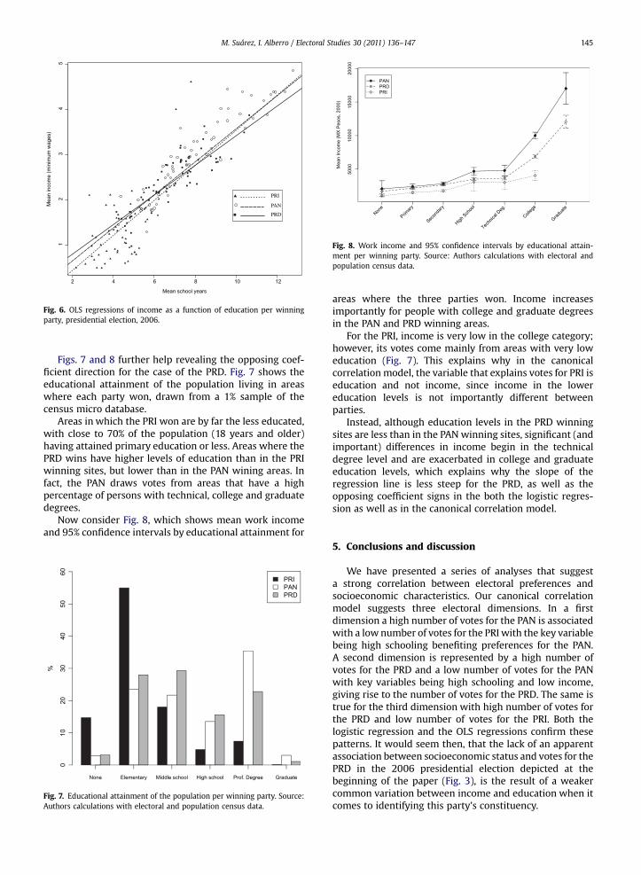
Figs. 7 and 8 further help revealing the opposing coef-ficient direction for the case of the PRD. Fig. 7 shows theeducational attainment of the population living in areaswhere each party won, drawn from a 1% sample of thecensus micro database.

Areas in which the PRI won are by far the less educated,with close to 70% of the population (18 years and older)having attained primary education or less. Areas where thePRD wins have higher levels of education than in the PRIwinning sites, but lower than in the PAN wining areas. Infact, the PAN draws votes from areas that have a highpercentage of persons with technical, college and graduatedegrees.

Now consider Fig. 8, which shows mean work incomeand 95% confidence intervals by educational attainment for

None Elementary Middle school High school Prof. Degree Graduate

%

001

0203

0405

06

PRIPANPRD

Fig. 7. Educational attainment of the population per winning party. Source:Authors calculations with electoral and population census data.

areas where the three parties won. Income increasesimportantly for people with college and graduate degreesin the PAN and PRD winning areas.

For the PRI, income is very low in the college category;however, its votes come mainly from areas with very loweducation (Fig. 7). This explains why in the canonicalcorrelation model, the variable that explains votes for PRI iseducation and not income, since income in the lowereducation levels is not importantly different betweenparties.

Instead, although education levels in the PRD winningsites are less than in the PAN winning sites, significant (andimportant) differences in income begin in the technicaldegree level and are exacerbated in college and graduateeducation levels, which explains why the slope of theregression line is less steep for the PRD, as well as theopposing coefficient signs in the both the logistic regres-sion as well as in the canonical correlation model.

5. Conclusions and discussion

We have presented a series of analyses that suggesta strong correlation between electoral preferences andsocioeconomic characteristics. Our canonical correlationmodel suggests three electoral dimensions. In a firstdimension a high number of votes for the PAN is associatedwith a lownumber of votes for the PRI with the key variablebeing high schooling benefiting preferences for the PAN.A second dimension is represented by a high number ofvotes for the PRD and a low number of votes for the PANwith key variables being high schooling and low income,giving rise to the number of votes for the PRD. The same istrue for the third dimension with high number of votes forthe PRD and low number of votes for the PRI. Both thelogistic regression and the OLS regressions confirm thesepatterns. It would seem then, that the lack of an apparentassociation between socioeconomic status and votes for thePRD in the 2006 presidential election depicted at thebeginning of the paper (Fig. 3), is the result of a weakercommon variation between income and education when itcomes to identifying this party’s constituency.

M. Suárez, I. Alberro / Electoral Studies 30 (2011) 136–147146

From the evidence presented in the paper, it can beclearly stated that preference for the PAN is associated withhigher income and education. It can also be clearly statedthat the preference for the PRI is associated with lowereducation and income. In the case of the PRD our analysessuggest that the preference for this partydat the same levelof educationdis associated with income levels that arelower than that of areas where people mainly vote for PANand the PRI.

The explanations for these patterns are straightforwardand well known regarding the preferences for the PAN andthe PRI, but subject to discussion in the case of the PRD.Historically the PAN has drawn its support from the middleclasses (Loaeza, 1988) who tend to have higher levels ofeducation and income than those belonging to morepopular sectors. The strengthening of the party that wouldlater become the PRI in the hands of Cárdenas implied themarginalization of the middle and upper classes. Loaezarefers to this process as a traumatic experience for thesesocial groups. The Partido Nacional Revolucionario (PNR),predecessor of the PRI, relied on the support of workers andpeasants and a corporatist structure around which thepolitical and social life of the country was structured.

Decades later we still observe that the social cements ofthe PRI remain although this party has lost popularity withsome groups mainly as a result of economic crisis that haveeroded the capability of greasing the electoral machinery.In turn the PAN, founded in 1939, was capable of rallyingthe support of youngsters issued from the middle classesand its main figure Manuel Gómez Morin became a strongcritic of the Cardenista regime. As opposition party duringseven decades, the PAN remained the party of choice ofthese middle and upper classes that had been explicitlymarginalized from the corporatist structure established byCárdenas and pivotal for the survival of the PRI.

In regards to our main finding, namely that the PRDdraws votes from areas where given the same level ofeducation, income is lower, we find two complementaryexplanations. On the one hand, voters who favored the PRDprofoundly disagreed with the Fox administration and itsperformance (48.4% of them disagree according to the 2006exit poll elaborated by Consulta Mitofsky, 2006). The 2006PRD voters were very critical of the administration andclearly wanted a change in the direction that the countrycould adopt, which could obviously be offered by the leftleaning party proposal.

In that sense, at least half of the voters who favored thePRD was punishing the ruling party and wanted a drasticchange. At the same time, we observe that those who votedfor the PRD had lower incomes than other voters (77% ofthem perceived less than three minimum wages accordingto Consulta Mitosfky), a fact that would be coherent withthe extensive literature proving that economic downturnslead to punishing through vote (Fiorina and Shpesle, 1990;Lau, 1985; Quattrone and Tversky, 1988). PRD voters havea history of protest through vote and 2006 was not theexception. At the time of its creation in 1988, the PRDseverely questioned the poor economic performance of thePRI administrations and demanded a more democraticpolitical system as well as a change in the status quo(Ortega, 2008). In the 2006 election PRD voters expressed

their feelings of relative deprivation and general dissatis-faction at the ballot box.

On the other hand, the fact that income and educationdo not move in the same direction in the case of the vote forthe PRD may well be the result of the occupational struc-ture. The Mexican economy has not been able to placenewly educated professionals in the formal job market,creating pockets of discontent and thus a fertile ground foropposition votes. This could also be the case for lesseducated areas where people feel they should be doingbetter economically speaking, but current federal govern-ment policies have done little to better their situation. Forthese groups of persons, that are geographically aggre-gated, there might be an interest in the left-wing economicmodel that favors more state intervention and socialprotection such as the one that the PRD offers.

The hypothesis presented above are consistent with thefact that those who voted for the PRD in the 2006 electionidentified poverty and unemployment as their mainconcerns while these problems were only secondary forvoters who favored other parties. Indeed, poverty wassignaled as themain problem facing the country by 34.9% ofthe PRD voters while unemployment was the mostimportant issue for 32.7% of them. In general, thesupporters of the PRD have a lower income than theircounterparts and a strong conviction that the countryoverall should be doing better and that their personalsituation should also improve.

This article represents in that sense an interestingcontribution on the socioeconomic determinants of parti-sanship. Although the literature to date has mostly focusedon the role of income and education and their relativeimportance in explaining turnout and preferences, there isstrong consensus that these two variables tend to influencethe outcome in the same direction and thus go hand inhand. This empirical study of the 2006 Mexican electionshows that in the case of the preferences for the left-wingpartydthe PRDdeducation is a key factor but whenever itis accompanied by higher levels of income, the likelihood ofsupport diminished. Income in turn tends to favor the PAN.

The analysis we have performed has certain limitations.First, it is limited because of the use of aggregate data. Thistype of information does not allow inferring the choices ofindividuals, only to understand general voting behavior.Our research is also limited by the fact that we look only atone election. Further research should address whether thepatterns we have found for the 2006 election hold for otherelectoral periods, for presidential and legislative votes.Analyzing mayoral elections would also contribute tofurther understand the relationship between Mexicansocioeconomic characteristics and partisanship. Still, webelieve that this study is a contribution in terms of itsmethodological innovationdthe use of a canonical modelto study turnoutdand the elaboration of a much moredetailed data set that gives us a closer geographical look atturnout at the GIS neighborhood level. This is an attractiveway to further elucidate voting behavior, to isolate regionaleffects and to understand the impact of different inde-pendent variables on partisanship especially in the case ofMexico as well as new democracies where electoral studiesstill require in depth analysis.

M. Suárez, I. Alberro / Electoral Studies 30 (2011) 136–147 147

At a time where there is a clear uprise of Latin Americangovernments from the left, especially in countries likeVenezuela, Ecuador and Brazil, it becomes even morerelevant to question if the constituencies of left leaningparties have a different –and more complexdrelationshipwith income and education than the constituencies thatfavor other parties. This paper provides an analysis in thatsense that can promote a better understanding of electoralpolitics in Mexico and provide a methodological basis forrich comparative studies.

Acknowledgements

The authors would like to thank Robert Work for hiscareful revision and suggestions on this paper.

References

Alberro, I., 2007. Do the poor go to the voting booth? A reevaluation of thesocioeconomic model of turnout in established and emergingdemocracies. Ph.D. dissertation, Northwestern University.

Almond, Gabriel, A., Sidney Verba, 1963. The Civic Culture. Political Atti-tudes and Democracy in Five Nations. Princeton University Press,Princeton, New Jersey, pp. 375.

Ames, B., 1970. Bases of support for Mexico’s Dominant party. TheAmerican Political Science Review 64 (1), 153–167.

Barber, J.D., 1969. Citizen Politics (Markham, Chicago).Barnes, Samuel, H., Max Kaase, 1963. Political Action: Mass Participation

in five Western Democracies. Sage Publications., Beverly Hills.California, pp. 607.

Bennett, S.E., Klecka, W.R., 1970. Social status and political participation:a multivariate analysis of predictive power. Midwest Journal ofPolitical Science 14 (2), 355–382.

Campbell, A., Converse Philip, E., Miller, W.E., Stokes, D.E., 1960. TheAmerican Voter. Wiley, New York.

CONAPO, 2005a. Indicadores Sociodemográficos, 2000@www.conapo.gob.mx.CONAPO, 2005b. Indicadores Sociodemográficos, 2005 @ www.conapo.

gob.mx.Consulta Mitofsky, 2006. www.consulta.com.mx.Cortina, J., Lasala Blanco, N., Gelman, A., 2010. One Vote, Many Mexico’s:

Income and Region in the 1994, 2000, and 2006 Presidential ElectionsUnder Review.

Cruz Rodriguez, María Soledad, 2001. Propiedad, poblamiento y periferiarural en la Zona Metropolitana de la Ciudad de México, Mexico,PERIU, UAM-A.

Eckstein, S., 1977. The Poverty of Revolution. The State and the Urban Poorin Mexico. Princeton University Press, Princeton, p. 301.

Fiorina, M., Shpesle, K., 1990. Negative voting: an explanation based onprincipal-agent theory. In: Ferejohn, J., Kuklinki, J. (Eds.), Informationand the Democratic Process. Urbana University: University of IllinoisPress.

Frank, T., 2004. What’s the Matter with Kansas? How Conservatives Wonthe Heart of America. Henry Holt and Company, LLC, New York.

Gelman, Andrew, et al., 2008. Red State, Blue State, Rich State, Poor State.Why Americans vote the way they do. Princeton University Press,Princeton, New Jersey, pp. 238.

Gelman, A., Kenworthy, L., Su, Yu-Sung, 2010. Income Inequality andpartisan voting in the US. Social Science Quarterly.

González Casanova, 1965. La Democracia en México. Ediciones Era,México D.F.

INEGI, 2000 XII Censo de población y vivienda 2000, Mexico, INEGI.Instituto Federal Electoral, 2006. Boletin 09. http://pac.ife.org.mx/notas/

09/pac_nota_participacion.html.Klesner, J., 1993. Modernization, economic crisis, and electoral alignment

in Mexico. Mexican Studies/Estudios Mexicanos 9 (2), 187–224.Klesner, J., 1998. Electoral alignment and the new party system in Mexico.

Documento presentado en el “Congress of the Latin American StudiesAssociation” (Chicago, IL).

Klesner, J.L., Lawson, C., 2001. ‘Adios’ to the PRI? Changing voter turnoutin Mexico’s political Transition. Mexican Studies/Estudios Mexicanos17 (1), 17–39.

Lau, R., 1985. Two explanations of Negativity effects in political behavior.American Journal of Political Science 29, 119–138.

Lawson, C., 2006. How did we get here? Mexican democracy after the2006 elections. Forthcoming. Political science and politics.

Loaeza, S., 1988. Clases medias y política en México. El Colegio de México,México.

Milbrath, L.W., 1965. Political Participation. Rand McNally, Chicago.Milbrath, L.W., Goel, M.L., 1977. Political Participation, second ed. Rand

McNally, Chicago.Molinar, J., Weldon, J., 1990. Elecciones de 1988 en México: crisis del

autoritarismo. Revista Mexicana de Sociología 52 (4), 229–362.Moreno, A., 2003. Democracia, Actitudes Políticas Y Conducta Electoral.

México: Fondo de Cultura Económica, México D.F.Moreno, A., Jan 2007. The 2006 Mexican presidential election: the

economy, Oil Revenues, and Ideology. PS: Political Science and Politics40, 15–19.

Ortega, R., 2008. Movilización Y Democracia España Y México. El Colegiode México, México D.F.

Quattrone, G., Tversky, A., 1988. Contrasting rational and psychological anal-ysis of political choice. American Political Science Review 82, 719–736.

Suárez, M., Delgado, J., 2009. Is Mexico city polycentric? A trip attractioncapacity approach. Urban Studies 46 (10), 2187–2211.

Verba,S.,Nie,N.H.,1972.Participation inAmerica.HarperandRow,NewYork.Verba, S., Norman,H.N.,Kim, Jae-On,1978. Participation andPolitical Equality:

a Seven Nation Comparison. Cambridge University Press, Cambridge.Vilalta, C., 2006. Sobre la Espacialidad de los Procesos Electorales Urbanos

y una Comparación entre las Técnicas de Regresión OLS y SAM.Estudios Demográficos Y Urbanos 21 (1), 83–122.