analyzing data from small n designs using multilevel models · analyzing data from small n designs...
TRANSCRIPT

Analyzing Data from Small N Designs Using Multilevel Models:
A Procedural Handbook
Eden Nagler, M.Phil
The Graduate Center, CUNY
David Rindskopf, PhD Co-Principal Investigator
The Graduate Center, CUNY
William Shadish, PhD Co-Principal Investigator
University of California - Merced Granting Agency: U.S. Department of Education Grant Title: Meta-Analysis of Single-Subject Designs Grant No. 75588-00-01
November 19, 2008

Analyzing Data from Small N Designs Using Multilevel Models: A Procedural Handbook
SECTION I. Introduction The purpose of this handbook is to clarify the steps in analyzing data from small-n designs using multilevel models. Within the manual, we have illustrated the procedures taken to conduct the analysis of a single-subject design small-n study of various single- and multiple-phase designs. Although we attempt to discuss our work in detail, readers should have some acquaintance with multilevel models (also called hierarchical models, or mixed effects models). The conceptual basis of these analyses is:
• Write a statistical model to summarize the behavior of each person • Test whether there are differences among people in various aspects of their
behavior; and if so • Test whether those differences are predicted by subject characteristics.
While searching through the literature for appropriate single-subject design studies to serve as pilots for this handbook, we looked to identify studies that adhered to several guidelines: Studies should include full graphs for at least 4 or 5 subjects Counts and/or measures displayed (as the dependent measure) should not be aggregated Data provided are as close to raw as possible
These demonstration datasets lead from simple to more complex designs and from simpler to more complex models. We begin with one-phase, treatment-only designs and continue through to four-phase ABAB reversal design studies. We demonstrate how to scan in graphed data and how to extract raw data from those graphs using computer software. We talk about how to deal with different types of dependent variables which require different statistical models (e.g., continuous, count or rate, proportion). Additionally, this type of data often contains autocorrelation. We also discuss this problem and one way of dealing with it. In Section II, we introduce procedures via demonstration with a dataset from a one-phase,
treatment-only study of a weight loss intervention where the outcome variable is a continuous variable. Here, we cover the following:
o Scanning graphs into Ungraph o Using Ungraph to extract raw data from graphs into spreadsheet (line graph) and then
export data into SPSS o Using SPSS to refine and set up data for HLM o Using HLM to set up a summary (mdm) file, specify and run models with a continuous
dependent variable (and both linear and quadratic effects), and create graphs of models
Section I – pg. 1

o Interpreting output In Section III, we expand the demonstration with a dataset from a two-phase (AB) design
study of a prompt-and-praise intervention for toddlers where the outcome variable is a count or rate. New material covered in this section includes the following:
o Introduction of Poisson distribution (prediction on a log scale), including a discussion of technical issues associated with a count as the DV (Poisson distribution, many zeros, using a log scale, etc)
o Using Ungraph to read in a scatterplot o Using HLM to set up and run a model to accommodate a rate as a DV o Interpreting HLM output with prediction on a log scale o Technical discussions of the following:
Considering the contribution of subject characteristics (L2 predictors) Exploring whether one subject stands out (when baseline for that subject is always
zero; comparing across alternative models) Constraining random effects (restricting between-subject variation to 0) and
comparing across models Exploring heterogeneity of Level-1 variance across phases (within-subject
variation) and comparing across models In Section IV, we further expand the demonstration with a dataset from a two-phase (AB)
design study of a collaborative teaming intervention for students with special needs where the outcome variable is a proportion (i.e., successes/trials). New material covered in this section includes the following:
o Introduction of Binomial distribution (prediction on a log odds scale) o Using SPSS to set up data for use of Binomial distribution model o Using HLM to set up model for a variable distributed as Binomial; set option for
Overdispersion, and run models as Binomial o Interpreting HLM output with prediction on a log odds scale o Technical discussion and demonstration on Overdispersion (including comparing across
models) Finally, in Section V, we demonstrate the steps with a dataset from a four-phase (ABAB)
reversal design study of a response card intervention for students exhibiting disruptive behavior where the outcome variable is again a proportion. New material covered in this section includes the following:
o Introduction of analyses of four-phase designs, including consideration of phase order o Using SPSS to set up data for use for a four-phase model, to test order effects and various
interactions o Using HLM to set up a model for the four-phase design, using the Binomial distribution,
testing order effects and various interactions o Special coding possibilities for a four-phase design o Interpreting HLM output from this type of design
Section I – pg. 2

SECTION II. One-Phase Designs One published study was selected to serve as an example to be used throughout this section:
Stuart, R.B. (1967). Behavioral control of overeating. Behavior Research & Therapy, 5, (357-365).
In this study, eight obese females were trained in self-control techniques to overcome overeating behaviors. Patients were weighed monthly throughout the 12-month program and these data were graphed individually. Data and graphs from this study will be used to illustrate various steps in the analysis discussed in this manual. The following pages will illustrate the steps necessary to get the data from print into HLM, to do an analysis, and interpret the output. These procedures utilize three computer packages: Ungraph, SPSS, and HLM. Screen shots are pasted within the instructions. Outline of steps to be covered: 1. Scan graphs into Ungraph 2. Define graph space in Ungraph 3. Read data from image to data file in Ungraph 4. Export data file into SPSS 5. Refine data as necessary in SPSS (recodes, transformations, merging Level-1 files, etc.) 6. Set up data in HLM (including setting up MDM file) 7. Run multilevel models in HLM 8. Create graphs of data and models in HLM 9. Interpret HLM output
Section II – pg. 1

Getting Data from Print into Ungraph
I. Scanning data to be read into Ungraph (via flatbed scanner):
1. Scan graphs into jpeg (or .emf, .wmf, .bmp, .dib, .png, .pbm, .pgm, .ppm, .pcc, .pcx, .dcx, .tiff, .afi, .vst, or .tga) format through any desired scanning software.
2. Save image of graph (e.g., to Desktop, My Documents folder, CD, flash drive, etc.) and
label for later retrieval. Example: Scanned Stuart (1967) graphs for each patient; all are in one jpeg file.
Next: Defining graph space in Ungraph
Section II – pg. 2

II. Defining graph space in Ungraph:
1. Start the Ungraph program.
(Note: If Ungraph was originally registered while connected to the Internet, then it will only open [with that same password] while connected to the Internet each time. It does not have to be connected at the same Internet port, just any live connection.)
2. Open the scanned image(s) in Ungraph:
Select File Open Browse to the intended image (scanned graph) and click Open so that the graph(s) is
displayed in the workspace. Scroll left/right, up/down to get the first subject’s graph fully visible in the
workspace. Use View Zoom In/Out as needed to optimize the view.
Example: Stuart (1967) – Patient 1 opened in Ungraph.
Section II – pg. 3

3. Define measures:
Select Edit Units Label X and Y accordingly (using information from the scanned graphs or the study
documentation) and click OK.
In our example, X is months and Y is lbs.
Example: Stuart (1967) – Patient 1 – defining units.
4. Define the Coordinate System:
Select Edit Define Coordinate System The program requires that you define 3 points for each graph. These do not have to be
points on the data line. In fact, you can be more precise if you choose points on the axes. Choose points that are relatively easily definable.
1. First scaling point – click on labeled point most to the right on the Y axis
(X=max, Y=min).
1
Section II – pg. 4

Example: Stuart (1967) – Patient 1 – First Scaling Point defined (1)
2. Deskewing point – this point must have the same Y value as above, so click on the intersection of the axes (which may or may not be the origin) (X=min, Y=min).
Example: Stuart (1967) – Patient 1 – D
2
eskewing Point defined (2)
Section II – pg. 5
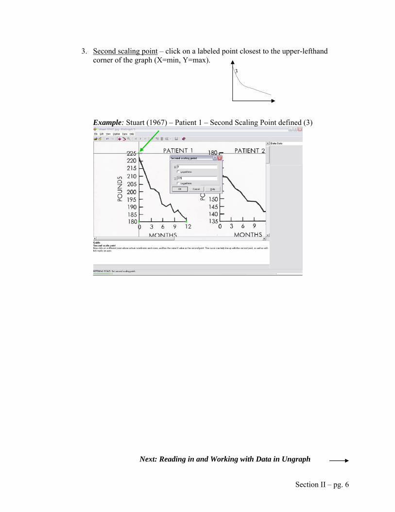
3. Second scaling point – click on a labeled point closest to the upper-lefthand corner of the graph (X=min, Y=max).
Example: Stuart (1967) – Patient 1 – Second Scaling Point defined (3)
3
Next: Reading in and Working with Data in Ungraph
Section II – pg. 6

III. Reading in & Working with data in Ungraph:
1. Reading data from graph:
If working with a line graph:
Select Digitize New Functional Line
Carefully click on left-most point on the graph line (on the Y axis) and watch Ungraph trace the line to the end. If the digitized line runs off beyond the actual line, you can click ALT
+ left-arrow ( ) to back up the digitization little by little You may need to try this step a few times before Ungraph follows the
line precisely. Click Undo (at bottom of screen) to erase any incorrectly-digitized line and start again.
Example: Stuart (1967) – Patient 1 – Digitize Functional Line
If the data are in a scatterplot:
Select Digitize New Scatter Carefully click on each data point in the graph to read in data
2. Working with extracted data:
Data values are computed as if they were collected continuously. For instance, even if data were actually collected once per month,
Ungraph may still show points for non-integer X values (e.g.,: 1.13 months, etc.), falsely assuming continuity.
Section II – pg. 7
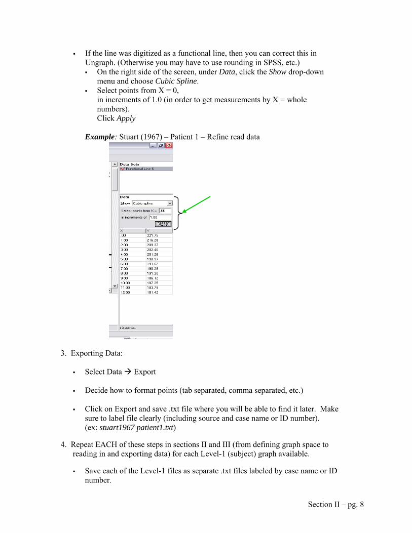
If the line was digitized as a functional line, then you can correct this in Ungraph. (Otherwise you may have to use rounding in SPSS, etc.) On the right side of the screen, under Data, click the Show drop-down
menu and choose Cubic Spline. Select points from X = 0,
in increments of 1.0 (in order to get measurements by X = whole numbers). Click Apply
Example: Stuart (1967) – Patient 1 – Refine read data
3. Exporting Data:
Select Data Export Decide how to format points (tab separated, comma separated, etc.)
Click on Export and save .txt file where you will be able to find it later. Make
sure to label file clearly (including source and case name or ID number). (ex: stuart1967 patient1.txt)
4. Repeat EACH of these steps in sections II and III (from defining graph space to reading in and exporting data) for each Level-1 (subject) graph available.
Save each of the Level-1 files as separate .txt files labeled by case name or ID
number.
Section II – pg. 8

Getting Data from Ungraph into SPSS
IV. Importing and Setting Up Level-1 Data in SPSS:
1. Open SPSS program.
2. Read text (.txt) file into SPSS:
Select File Read Text Data Browse to first Level-1 text (.txt) file (Patient 1)
Click Next 3 times (or until you get to the screen below)
At the screen that asks “Which delimiters appear between variables?”
(Delimited Step 4 of 6), check off whichever delimiters you specified when exporting data from Ungraph (tab, comma, etc).
Example: Stuart (1967) – Patient 1 – Reading text file into SPSS
Click Next to advance to the next screen Title variables:
Click on column V1 and enter name of variable; repeat for other variables.
Section II – pg. 9

Example: Stuart (1967) – Patient 1 – Reading text file into SPSS
Click Next to advance to the next screen Finally, click Finish to complete set-up of text data.
Example: Stuart (1967) – Reading text data into SPSS.
Section II – pg. 10

3. Dataset should now be displayed in Data View screen.
Title/label variables as necessary in Variable View. 4. Compute subject’s ID for data:
For this study, we computed Patient ID for each subject by running the following syntax (where the value “1” is changed for each subject respectively):
COMPUTE patient=1.
EXECUTE.
5. Save individual subject SPSS data files:
Save the SPSS data file for the first “patient” (in this study). Make sure to include the subject’s ID in the file name so that you will be able to identify it later. (ex: stuart1967 patient1.sav)
6. Repeat steps 1 through 5 above for each subject in the study (for each of the text files created from each of the graphs scanned) creating separate Level-1 files for each subject/patient/unit.
Be sure to compute appropriate subject ID’s for each subject.
For example, in the study used in this manual, we ended up with 8
separate Level-1 files. In the first, we computed patient=1, in the second, we computed patient=2,… and so on… until the eighth, when we computed patient=8.
As well, each file was saved with the same file name except for the
corresponding patient ID.
7. Now that you have uniform SPSS files for each subject, you must merge them. Merge data files for each subject into one Level-1 file. (Select Data Add cases, etc.)
8. Sort by subject ID.
Section II – pg. 11

Example: Stuart (1967) – Merged Level-1 SPSS file.
9. In the merged file, you may wish to make additional modifications to the
variables. For this dataset, we decided to make three such modifications/transformations:
First, we rounded “lbs” to the nearest whole number, with the following
syntax command:
COMPUTE pounds = rnd(lbs). EXECUTE.
Second, for more meaningful HLM interpretation, we decided to recode months so that 0 represented ending weight, instead of starting weight. We did this with the following syntax command:
COMPUTE months12 = months-12. EXECUTE.
Last, we computed a quadratic time term (months2) so that we may later test for a curvilinear trend when working in HLM. We ran the following syntax to compute this variable:
COMPUTE mon12sq = months12 ** 2. EXECUTE.
Section II – pg. 12

10. For some models, you will need to create indicator variables. See HLM 6 Manual
– Chapter 8. 11. After making all modifications and sorting by ID, re-save complete Level-1 file.
Example: Stuart (1967) – Complete Merged Level-1 SPSS file.
Next: Setting up Level-2 data in SPSS
V. Entering and Setting Up Level-2 Data in SPSS 1. Create SPSS file including any Level-2 data (subject characteristics) available:
Make sure to use corresponding subject IDs to those set up in Level-1 file.
There should be one row for each subject.
Section II – pg. 13

There should be one column for subject ID. Remember to use corresponding IDs to the Level-1 file. Also, variable name, type, etc should match Level-1 set-up of the ID variable.
Other columns should include data revealed in the study about each subject.
For example, in this study, we had data on Age, Marital Status, Total
Sessions attended, and Total Weight Loss.
2. You may decide later to go back and recenter or redefine these variables for more meaningful HLM interpretation.
For example, in this dataset, the average age of a subject was just above
30. In order to allow for simpler interpretation, we computed Age30 = age-30, so that Age30=0 would represent a person of about average age.
Example: Stuart (1967) – Level-2 Dataset in SPSS
Next: Getting data into HLM
Section II – pg. 14

Getting Data from SPSS into HLM
In this section, we discuss the simplest models that do not use indicator variables. In a later section, we will consider other models for the covariance structure. VI. Setting up MDM file: (Note: For HLM versions 5 and below, create an SSM file; for versions 6 and higher, create an MDM file.)
1. Open HLM program. (Make sure all related SPSS files are saved and closed.)
2. Select File Make new MDM file Stat package input Example: Stuart (1967) – Setting up new MDM.
3. On next window, leave HLM2 bubble selected and click OK. Example: Stuart (1967) – Setting up new MDM.
Section II – pg. 15

4. Label MDM file:
At top right of Make MDM screen, enter MDM file name, making sure to end in .mdm. Example: “stuart1967.mdm”
Make sure that Input File Type indicates SPSS/Windows.
5. Specify structure of data:
In this case, our data was nested within patients so under Nesting of input data we selected measures within persons.
6. Specify Level-1 data:
Under Level-1 Specification, click on Browse and browse to saved Level-1 SPSS file (the merged one). Click Open.
Once your Level-1 file has been identified, click on Choose Variables.
Check off your subject ID variable as ID.
Check off all other wanted variables as in MDM.
Click OK.
Example: Stuart (1967) – Choosing variables for Level-1 data.
Section II – pg. 16

7. Specify Level-2 data:
Under Level-2 Specification, click on Browse and browse to saved Level-2 SPSS file. Click Open.
Once your Level-2 file has been identified, click on Choose Variables.
Check off your subject ID variable as ID.
Check off all other wanted variables as in MDM.
Click OK.
Example: Stuart (1967) – Choosing variables for Level-2 data.
8. Save Response File:
On top left of Make MDM screen, click Save mdmt file. Name file and click Save.
9. Make MDM:
On bottom of screen, click on Make MDM. A black screen will appear and then close.
Section II – pg. 17

10. Check Stats:
On bottom of screen, click Check Stats. Examine descriptive statistics as a preliminary check on data.
11. Done:
Click on Done.
Next: Running Multilevel Models in HLM
Section II – pg. 18

Running Multilevel Models in HLM (Linear and Quadratic) VII. Setting up the model:
As evident from the graphs, each person lost weight at a fairly steady rate. We first fit a straight line for each person, allowing the slopes and intercepts to vary across people. Late, we test whether a curve would better describe the loss of weight over time.
LINEAR MODEL -
With MDM file (just created) open in HLM, 1. Choose outcome variable:
With Level-1 menu selected, click on POUNDS and then Outcome variable to
specify weight as outcome measure. Example: Stuart (1967) – Setting up models in HLM
Identify which Level-1 predictor variables you want in the model. (Often, the only such predictor variable will be a time-related variable.):
Click on MONTHS12 (or whichever variables you want in the Level-1
equation) and then add variable uncentered.
Section II – pg. 19

Example: Stuart (1967) – Setting up models in HLM
3. Activate Error terms: Make sure to activate relevant error terms (depending on model) in each
Level-2 equation by clicking on the error terms individually (r0 is included by default; others much be selected).
In this case, we activated all Level-2 error terms.
Example: Stuart (1967) – Setting up models in HLM
Section II – pg. 20

4. Title output and graphing files:
Click on Outcome
Fill in Title (this is the title that will appear printed at the top of the output text file).
Fill in Output File Name and location (this is the name and location where the output file will be saved); and Graph File Name and location (this is the name and location where the graph file will be saved).
Click OK to save these specifications and exit this screen. Example: Stuart (1967) – Setting up models in HLM
5. Exploratory Analysis:
Select Other Settings Exploratory Analysis (Level-2) Example: Stuart (1967) – Setting up Exploratory Analysis.
Section II – pg. 21

Click on each Level-2 variable that you want to include in the exploratory
analysis and click add. (In this case, we selected age30, marital status, and total sessions.):
Example: Stuart (1967) – Setting up Exploratory Analysis.
Click on Return to Model Mode at top right of screen.
6. Run the analysis
At the top of the screen, click on Run Analysis.
On the pop-up screen, click on Run model shown. Example: Stuart (1967) – Setting up Exploratory Analysis.
Section II – pg. 22

A black screen will appear, and then close. 7. View Output:
Select File View Output
Output text file will open in Notepad.
Note: You may also open the output file directly by browsing to its saved location (specified in Outcome menu) from outside HLM.
Example: Stuart (1967) – HLM output text file.
Section II – pg. 23
QUADRATIC MODEL The quadratic model was set up just like the linear model EXCEPT for the following: When defining the variables in the model, we also included MON12SQ (the quadratic
term) in the Level-1 equation. In the Exploratory Analysis, we requested the same Level-2 variables to be explored
in each of the equations, now also including the quadratic term equation. File names and titles were changed to identify this as the quadratic model.
Creating Graphs of the Data and Models in HLM
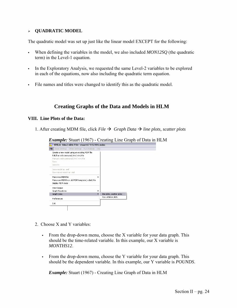
VIII. Line Plots of the Data: 1. After creating MDM file, click File Graph Data line plots, scatter plots
Example: Stuart (1967) - Creating Line Graph of Data in HLM
2. Choose X and Y variables:
From the drop-down menu, choose the X variable for your data graph. This should be the time-related variable. In this example, our X variable is MONTHS12.
From the drop-down menu, choose the Y variable for your data graph. This
should be the dependent variable. In this example, our Y variable is POUNDS. Example: Stuart (1967) - Creating Line Graph of Data in HLM
Section II – pg. 24

3. Select number of groups to display in graph:
From the drop-down menu at the top-right of the window, select the number
of groups to display. In this example, we are actually selecting the number of individuals for whom the graph will display nested measurements. Choose All groups (n=8).
Example: Stuart (1967) - Creating Line Graph of Data in HLM
4. Select Type of Plot: Under Type of plot, select Line plot and Straight line.
5. Select Pagination:
Section II – pg. 25

Under Pagination at bottom-right of screen, select All groups on same graph.
Example: Stuart (1967) - Creating Line Graph of Data in HLM
6. Click OK to make line plot of data.
Example: Stuart (1967) - Creating Line Graph of Data in HLM
IX. Line Plots of the Level-1 Model(s):
LINEAR MODEL GRAPHING
1. After running the linear model in HLM 6, Click File Graph Equations Level-1 equation graphing
Section II – pg. 26

Example: Stuart (1967) – Creating Line Graph of Linear Model
2. Select X focus variable:
From the drop-down menu, select the X focus variable for linear model graph. In this example, we chose MONTHS12.
Example: Stuart (1967) – Creating Line Graph of Linear Model
3. Select number of groups to display in graph: From the drop-down menu, select the number of groups to display. Choose
All groups (n=8).
Example: Stuart (1967) – Creating Line Graph of Linear Model
Section II – pg. 27

4. Click OK to get line graph of the linear prediction model. If the linear model is right, this describes the weight loss trajectory for each of the eight subjects.
Example: Stuart (1967) – Creating Line Graph of Linear Model
QUADRATIC MODEL GRAPHING
1. After running the quadratic model, Click File --> Graph Equations --> Level-1 equation graphing
Example: Stuart (1967) – Creating Line Graph of Quadratic Model
Section II – pg. 28

2. Select X focus variable:
From the drop-down menu, select the original X variable. (This will be further defined in a later step.) In this example, we chose MONTHS12.
Example: Stuart (1967) – Creating Line Graph of Quadratic Model
3. Select number of groups to display in graph: From the drop-down menu, select the number of groups to display. Choose
All groups (n=8).
Example: Stuart (1967) – Creating Line Graph of Quadratic Model
4. Specify relationship between original time variable (MONTHS12) and transformed/ quadratic time variable (MON12SQ).
Under Categories/transforms/interaction, click 1 and power of x/z to define
quadratic relationship.
Example: Stuart (1967) – Creating Line Graph of Quadratic Model
Section II – pg. 29

Choose transformed variable (in this case, MON12SQ) and define in terms of
original variable (here, MONTHS12 to the power of 2). Click OK.
Example: Stuart (1967) – Creating Line Graph of Quadratic Model
5. Click OK to get line graph of the quadratic prediction model. If the quadratic
model is right, this describes the weight loss trajectory for each of the eight subjects.
Section II – pg. 30

Example: Stuart (1967) – Creating Line Graph of Quadratic Model
Section II – pg. 31

Interpreting HLM Output
Note on typographic conventions Different fonts indicate different sources of information presented: Where we present our own interpretation and discussion, we use the Times New Roman font, as seen here. Where we present output from HLM, we use the Lucinda Console font, as used in the HLM Output text files opened in Notepad, and as seen here.
The Stuart (1967) study included data on eight subjects undergoing a weight loss program. Patients were weighed each month, and weight in pounds was recorded. Additional data were available on a few patient characteristics (e.g., age, marital status, total sessions attended). These variables had not been explored as potential explanatory factors in weight loss variations. Hierarchical linear modeling (HLM) was utilized to: (1) model the change in weight for each person, and (2) combine results of all women in the study so that we may examine trends across the study and between patients. Multiple observations on each individual (n=13 observations throughout the one-year treatment) were treated as nested within the patient. (We focus on statistical analysis here, but note that any inference about causal effect in this study requires strong assumptions. All patients received the same treatment, and there was no period to collect baseline data. Presumably these patients had stable weight for some long period of time before beginning treatment. Another implicit assumption is that most or all of the weight loss observed was due to treatment, and not to a “placebo” or Hawthorne effect, nor to natural changes in body chemistry.) A line graph, produced in SPSS, plotting weight in pounds by month of treatment for each patient is presented below. Each line represents the weight loss trend of one patient in the study over the 12-month treatment. The graph suggests that weight loss trends may not be uniform across patients (i.e., lines are not quite parallel). Hierarchical linear modeling (HLM) allow us to examine the significance of patient characteristics that may account for variations in weight loss slopes. As well, the line graph suggests that the line of best fit may not simply be linear but rather include a quadratic term to account for a slight curvature in the data. These speculations were examined and are discussed below.
Section II – pg. 32

Figure 1. Stuart (1967) – Line graph of weight loss by patient.
Weight Loss by Patient
(Stuart, 1967)
MONTHS12
0-1-2-3-4-5-6-7-8-9-10-11-12
PO
UN
DS
240
220
200
180
160
140
120
PATIENT
1
2
3
4
5
6
7
8
LINEAR MODEL – We initially chose the Stuart (1967) study to serve as a simple example in how to use HLM to analyze single subject studies. Though we later realized this data would not produce such a simple HLM interpretation (e.g., the need to include a quadratic term), we decided to discuss the simpler linear model as an introduction to the more complex model to follow. After setting up the MDM file, we identified POUNDS as the outcome variable and directed HLM to include MONTHS12 (computed previously in SPSS) in the model (uncentered). This resulted in a test of the model(s) displayed below. (These equations are from the HLM output and omit subscripts for observations and individuals.) Summary of the model specified (in equation format) --------------------------------------------------- Level-1 Model Y = P0 + P1*(MONTHS12) + E Level-2 Model P0 = B00 + R0 P1 = B10 + R1 The Level-1 equation above states that POUNDS (the weight for a patient at a particular time) is the sum of 3 terms: weight at the intercept (in this case, when MONTHS12=0, this is the ending weight), plus a term accounting for the rate of change in weight with time (MONTHS12), plus an error term. This simple linear model does not include any Level-2 predictors (patient characteristics). The Level-2 equations model the intercept and slope as:
Section II – pg. 33

P0 = The average ending weight for all patients (B00), plus an error term to allow each patient to vary from this grand mean (R0). P0 is the intercept of the regression line predicting weight from time.
P1 = The average rate of change in weight per month (MONTHS12) for the 8 participants (B10), plus an error term to allow each patient to vary from this grand mean effect (R1). Note: Remember that MONTHS12 was recoded so that 0=ending weight and -12=starting weight.
The following estimates were produced by HLM for this model: Final estimation of fixed effects: --------------------------------------------------------------- Standard Approx. Fixed Effect Coefficient Error T-ratio d.f. P-value --------------------------------------------------------------- For INTRCPT1,P0 INTRCPT2, B00 156.439560 5.053645 30.956 7 0.000 For MONTHS12 slope, P1 INTRCPT2, B10 -3.078984 0.233772 -13.171 7 0.000 --------------------------------------------------------------- The outcome variable is POUNDS When MONTHS12=0 (end of treatment), the overall average weight for all patients is 156.4396 (B00). This is the average ending weight for all patients. The average rate of change in weight per month (MONTHS12) is -3.0790 (B10); meaning that for each month in treatment (1-unit increase in MONTHS12), weight decreases, on average, just over 3 pounds. This decrease is statistically significant as the p-value for B10 is less than .05. Next, we must examine the variances of R0 and R1 (called taus in the HLM model) to determine if this average model fits suitably for all patients in the study. Final estimation of variance components: ---------------------------------------------------------------- Random Effect Standard Variance df Chi-square p-value Deviation Component ---------------------------------------------------------------- INTRCPT1, R0 14.23444 202.61939 7 843.67874 0.000 MONTHS12 slope,R1 0.63505 0.40329 7 90.26605 0.000 Level-1, E 2.48405 6.17052 ---------------------------------------------------------------- The between-patient variance on intercepts (again, in this case, the intercept is ending weight since MONTHS12=0 is end of treatment) is estimated to be 202.6194 (tau00), which corresponds to a standard deviation of 14.2344. The p-value shown tests the null hypothesis that ending weights for all patients are similar. The significant p-value (p<.001) indicates there is a significant amount of variation between patients on their ending weights. In other words, the variance is too big to assume it may be due only to
Section II – pg. 34
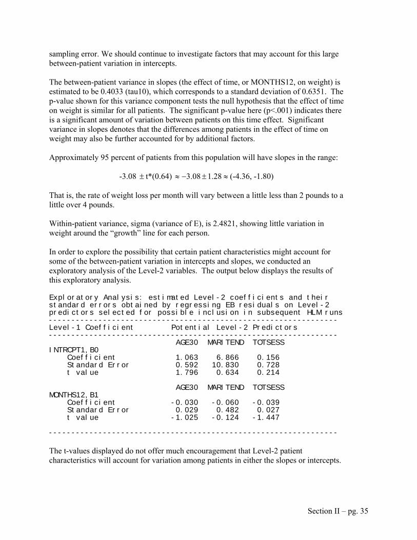
sampling error. We should continue to investigate factors that may account for this large between-patient variation in intercepts. The between-patient variance in slopes (the effect of time, or MONTHS12, on weight) is estimated to be 0.4033 (tau10), which corresponds to a standard deviation of 0.6351. The p-value shown for this variance component tests the null hypothesis that the effect of time on weight is similar for all patients. The significant p-value here (p<.001) indicates there is a significant amount of variation between patients on this time effect. Significant variance in slopes denotes that the differences among patients in the effect of time on weight may also be further accounted for by additional factors. Approximately 95 percent of patients from this population will have slopes in the range:
-3.08 t*(0.64) ± ≈±−≈ 28.108.3 (-4.36, -1.80) That is, the rate of weight loss per month will vary between a little less than 2 pounds to a little over 4 pounds. Within-patient variance, sigma (variance of E), is 2.4821, showing little variation in weight around the “growth” line for each person. In order to explore the possibility that certain patient characteristics might account for some of the between-patient variation in intercepts and slopes, we conducted an exploratory analysis of the Level-2 variables. The output below displays the results of this exploratory analysis. Exploratory Analysis: estimated Level-2 coefficients and their standard errors obtained by regressing EB residuals on Level-2 predictors selected for possible inclusion in subsequent HLM runs ---------------------------------------------------------------- Level-1 Coefficient Potential Level-2 Predictors ---------------------------------------------------------------- AGE30 MARITEND TOTSESS INTRCPT1,B0 Coefficient 1.063 6.866 0.156 Standard Error 0.592 10.830 0.728 t value 1.796 0.634 0.214 AGE30 MARITEND TOTSESS MONTHS12,B1 Coefficient -0.030 -0.060 -0.039 Standard Error 0.029 0.482 0.027 t value -1.025 -0.124 -1.447 ---------------------------------------------------------------- The t-values displayed do not offer much encouragement that Level-2 patient characteristics will account for variation among patients in either the slopes or intercepts.
Section II – pg. 35

In fact, further attempts at finding a better fitting model by including various patient characteristics (Level-2 variables) were not successful. In other words, no Level-2 variables in the data set could account for significant variation among patients in either the slopes or intercepts. Because we could not find a better fit of the linear model, and we had suspected that weight loss might have followed a curvilinear trend, we repeated the HLM analysis this time including a quadratic term for time (MON12SQ) in the Level-1 equation. QUADRATIC MODEL In order to explore the fit of a curvilinear trend in the data, we started with the same model as the simple linear equations discussed above but included an additional variable in the Level-1 model. We included MON12SQ (previously computed in SPSS), the squared time term, uncentered as well. This resulted in a test of the model displayed below. Summary of the model specified (in equation format) --------------------------------------------------- Level-1 Model Y = P0 + P1*(MONTHS12) + P2*(MON12SQ) + E Level-2 Model P0 = B00 + R0 P1 = B10 + R1 P2 = B20 + R2 The Level-1 equation states that a patient’s weight (POUNDS) is the sum of 4 quantities: weight at the end of treatment, the rate of weight loss toward the end of treatment (MONTHS12), the rate of change in this slope (MON12SQ), and an error term. The Level-2 equations model the intercepts and slopes (without any patient characteristics) as: P0 = The average ending weight for all patients (B00), plus an error term to allow each
patient to vary from this grand mean (R0). P0 is the intercept of the regression line predicting weight from time.
P1= The average rate of change in weight per month (MONTHS12) for all patients (B10) at the end of the study (near MONTHS12=0), plus an error term to allow each patient to vary from this grand mean effect (R1).
P2 = The average rate of change in slope for all patients (B20), plus an error term to allow for variation (R2).
The following estimates were produced for this model by HLM:
Section II – pg. 36

Final estimation of fixed effects: ---------------------------------------------------------------- Standard Approx. Fixed Effect Coefficient Error T-ratio d.f. P-value ---------------------------------------------------------------- For INTRCPT1, P0 INTRCPT2, B00 158.833791 5.321806 29.846 7 0.000 For MONTHS12 slope, P1 INTRCPT2, B10 -1.773039 0.358651 -4.944 7 0.001 For MON12SQ slope, P2 INTRCPT2, B20 0.108829 0.021467 5.070 7 0.001 ---------------------------------------------------------------- The outcome variable is POUNDS When we include the quadratic term, at MONTHS12=0 (end of treatment), the overall average weight for all patients is 158.8338 (B00). The average rate of change in pounds per month near the end of the study (MONTHS12) is -1.7730 (B10); meaning that toward the end of treatment, for each month in the program (1-unit increase in MONTHS12), weight decreases, on average, just less than 2 pounds. This decrease (effect) is statistically significant, as the p-value for B10 is less than .05. The average rate of change in this slope is 0.1088 (B20). In other words, the slope (or effect of time on weight loss) gets about 0.11 less steep per month. Patients lose the most weight per month towards the beginning of treatment, but this effect flattens out as treatment continues. The significant p-value (.001) indicates that this quadratic term adds an important piece to the prediction: There is, in fact, a curvilinear trend to be accounted for. Next, we must examine the taus to determine if this average model fits suitably for all patients in the study. Final estimation of variance components: ---------------------------------------------------------------- Random Effect Standard Variance df Chi-square P-value Deviation Component ---------------------------------------------------------------- INTRCPT1,R0 14.98754 224.62629 7 814.54023 0.000 MONTHS12 slope,R1 0.85863 0.73725 7 23.99148 0.001 MON12SQ slope, R2 0.04247 0.00180 7 12.85100 0.075 Level-1, E 1.94136 3.76889 ---------------------------------------------------------------- The between-patient variance on intercepts (ending weight) is estimated to be 224.6263 (tau00), which corresponds to a standard deviation of 14.9875. The between-patient variance on slopes (the effect of time, or MONTHS12, on weight) is estimated to be 0.7373 (tau11), which corresponds to a standard deviation of 0.8586. The significant p-value here (p=.001) indicates there is a statistically significant amount of
Section II – pg. 37

variation between patients on this time effect. In other words, at the end of 12 months, some are losing weight faster than others: approximately 95% have slopes between -1.77± 1.96*(.86) 1.77± 1.72 (-3.49, -.05). Some are losing weight as fast as almost 3.5 pounds per month and others are losing almost nothing.
≈ ≈
The between-patient variance on change in slopes (how much the rate of change of slopes varies, MON12SQ) is estimated to be 0.0018 (tau22). This is NOT statistically significant (p>.05), indicating we may not reject the null hypothesis that this curvilinear trend is the same across patients. Within-patient standard deviation, or sigma (σ), is 1.9413, slightly smaller than before, showing that we have accounted for slightly more variation in weight. In order to explore the possibility that certain patient characteristics might account for some of the significant between-patient variation in intercept (P0) and slope (P1), we conducted an exploratory analysis of the potential contributions of Level-2 variables. The output below displays the results of this exploratory analysis. Exploratory Analysis: estimated Level-2 coefficients and their standard errors obtained by regressing EB residuals on Level-2 predictors selected for possible inclusion in subsequent HLM runs ---------------------------------------------------------------- Level-1 Coefficient Potential Level-2 Predictors ---------------------------------------------------------------- AGE30 MARITEND TOTSESS INTRCPT1,B0 Coefficient 1.121 7.338 0.111 Standard Error 0.623 11.400 0.769 t value 1.799 0.644 0.144 AGE30 MARITEND TOTSESS MONTHS12,B1 Coefficient -0.001 0.197 -0.060 Standard Error 0.042 0.642 0.035 t value -0.019 0.307 -1.731 ---------------------------------------------------------------- Once again, the t-values displayed do not offer much encouragement that Level-2 patient characteristics will contribute anything significant to the prediction model. And again, further attempts at finding a better fitting quadratic model by including various patient characteristics (Level-2 variables) were not successful. In other words, no Level-2 variables added anything significant to the prediction. SUMMARY In the end, the best fitting model we could find included a quadratic term at Level-1 but no Level-2 predictors. This model is expressed by the following:
Section II – pg. 38

Level-1 Model Y = P0 + P1*(MONTHS12) + P2*(MON12SQ) Level-2 Model P0 = B00 + R0 P1 = B10 + R1 P2 = B20 + R2 with parameters estimated as: Coefficient (and p-value) Variance component (and p-
value) Intercept B00 = 158.8338 Tau00 = 224.6465, p<.001** Slope (MONTHS12) B10 = -1.7730, p = .001** Tau11 = 0.7373, p = .001** Quad. Term (MON12SQ)
B20 = 0.1088, p = .001** Tau22 = 0.0018, p = ns
The model for the average person (i.e., without error terms) is: Yij = 158.8338 – 1.7730*(MONTHS12) + 0.1088*(MON12SQ) Theoretically, it makes sense that patients in this study would lose weight at a faster rate at the beginning of treatment (when they were heavier) and at a slower (or flatter) rate towards the end of the one-year treatment (when they were lighter). Had we not explored the possibility of a quadratic term in the model, we would have instead used the average prediction equation, Yij = 156.4396 – 3.0790*(MONTHS12), which assumes that weight loss (slope) was constant throughout treatment. We can further verify the fit of the quadratic model over that of the linear model by visually examining the plots below.
Section II – pg. 39

Figure 2A. Actual data.
134.8
157.7
180.5
203.3
226.2
POU
ND
S
-12.60 -9.30 -6.00 -2.70 0.60
MONTHS12 Figure 2C. Quadratic Model Prediction
Figure 2B. Linear Model Prediction.
-12.00 -9.00 -6.00 -3.00 0137.8
157.2
176.7
196.2
215.7
MONTHS12
POU
ND
S
Yij = 156.4396 – 3.0790*(MONTHS12)
Yij = 158.8338 – 1.7730*(MONTHS12) + 0.1088*(MON12SQ)
-12.00 -9.00 -6.00 -3.00 0138.7
158.8
179.0
199.1
219.2
MONTHS12
POU
ND
S
We can see from these plots that the data (Figure 2A in the upper left-hand corner) seem slightly better fit by the quadratic model’s prediction beneath it (Figure 2C) than by the linear model’s prediction beside it (Figure 2B). This visual comparison gives us additional corroboration on selecting the quadratic model as the best fitting model.
Section II – pg. 40

SECTION III: Two-Phase Designs, Outcome = Rate An additional published study was selected to serve as an example throughout this section of the handbook. This example is used to: (1) show how to analyze data from a two-phase (AB) study; and, (2) illustrate ways of dealing with a count as a dependent variable and related issues that may arise during analysis and interpretation.
Dicarlo, C.F. & Reid, D.H. (2004). Increasing pretend toy play of toddlers with disabilities in an inclusive setting. Journal of Applied Behavior Analysis, 37(2), 197-207.
In this study, researchers observed the play behavior of five toddlers with disabilities. Observations took place in an inclusive classroom, over approximately forty 10-minute sessions, where the count of independent pretend toy play was tallied as the target behavior. The dependent variable in this dataset is a count, which must be accommodated in the analyses. Such accommodations will be discussed below. There were two phases in this study. For the first 16 to 28 sessions (depending on the subject), children were observed without intervention (baseline phase). For the remaining sessions, children were prompted and praised for independent pretend-play actions. This was the responsive teaching program, or treatment phase. Data must be coded so that count variations within and across the two phases can be examined. Phase coding will be discussed below. A series of line graphs, scanned and pasted from the original publication, plotting the count of play actions (Y) by session (X) for each subject, are presented below. For each, the data points to the left of the vertical line indicate observations made during the baseline phase and the points to the right of the vertical line indicate observations made during the treatment phase.
Section III – pg. 1

Figure III.1: DiCarlo & Reid (2004). Count of play actions by session and phase for subjects 1-5.
Because the dependent variable is a count (how many independent pretend toy play actions were observed in each interval), we used a Poisson distribution when analyzing the data (instead of a normal distribution). The Poisson is often used to model the number of events in a specific time period. We can see in the graphs above that across all subjects, in many sessions no pretend play actions were observed. In using a Poisson model, HLM will estimate the rate of behavior on a log scale; the log of 0 is negative infinity. This dependent variable zero trend, especially evident in the baseline phase, may then become a problem during analysis. More specific information about this problem and some potential ways of resolving it are discussed below. The graphs also suggest that changes or trends in count over sessions may not be uniform across students and that the treatment effect (or the change in intercept from baseline to treatment phase) may vary across students. Particularly, it looks like subject 3 (“Kirk”, the graph in the lower left-hand corner of the image) may not follow the same pattern as the other children. We will examine this inconsistency via HLM analyses by creating a dummy variable for this subject, and entering that dummy variable into the equation for treatment effect. We will examine whether or not such exploration is warranted and how it might be performed. Additional (Level-2) data were available on subjects’ chronological age and level of cognitive functioning. These variables had not been explored as potential explanatory factors in play action variation. We aimed to use hierarchical linear modeling (HLM) to: (1) model the change in the count of play actions for each child, (2) combine results of all students in the study so that we may examine trends across the study and between students, and, (3) model the change
Section III – pg. 2

in play action counts between phases. Multiple observations on each individual were treated as nested within the subject. Additionally, hierarchical linear modeling (HLM) will allow us to examine the significance of student characteristics (including a dummy variable indicating whether the child was Kirk or not) that may account for variations in intercepts and slopes. In order to perform such analyses and to simplify interpretation, several variables had to be recoded and/or created anew. Level-1 variable recodes and calculations include:
Phase was coded as 0 for baseline and 1 for treatment. (PHASE) Session was recentered so that 0 represented the session right before the phase
change. (SESSIONC) A variable for the session-by-phase interaction was computed by multiplying the
2 previous variables. (SESSxPHA = SESSIONC * PHASE) Level-2 variables also needed to be recoded and/or created:
Cognitive age was centered around its approximate mean, so that a cognitive age of 0 indicated a child of about average cognitive functioning for the sample. (COGAGE15)
Chronological age had to be extracted from the text of the study, as it was not overtly offered as data. (CHRONAGE)
A dummy variable for Kirk (subject 3) was created so that subject 3 had a 1 on this variable, and the remaining subjects had a 0. (KIRKDUM)
Therefore, a 0 on all Level-1 variables (session, phase, session-by-phase interaction) denotes the final baseline session. Intercepts for the computed models are then the predicted counts at the phase change. The full model (without any Level-2 predictors) is then: Level-1:
Log (FREQRNDij) = P0 + P1*(SESSIONC) + P2*(PHASE) + P3*(SESSxPHA) Level-2:
P0 = B00 + R0 P1 = B10 + R1 P2 = B20 + R2 P3 = B30 + R3
Details about how to create and/or transform the Level-1 and Level-2 variables are described below.
Section III – pg. 3

Getting Data from Print into Ungraph
I. Scanning data to be read into Ungraph (via flatbed scanner): Graphs from Dicarlo & Reid (2004) were scanned and saved in the same manner as previously explained. The diagram below displays the Dicarlo & Reid (2004) graphs as published. Example: Scanned Dicarlo & Reid (2004) graphs for each student.
Note: For each graph, you must decide if using Ungraph is worth your trouble. In this case, reading and entering data manually would probably have taken us the same amount of time as it did to use Ungraph to read in data (clicking on individual points, creating individual data files, and then merging data files back together). Regardless, we review this procedure, now with a scatterplot, for your consideration. II. Defining graph space in Ungraph:
Graph space was defined just as before: Open the scanned image(s) in Ungraph as before (File Open, scroll and zoom, etc.).
Define measures as before (Edit Units, label X and Y axes).
Section III – pg. 4

Define the Coordinate System as before (Edit Define Coordinate System, etc.).
Note: For this dataset, we defined the Y-axis scale as Count of Pretend Play Actions per Session, not average actions per minute, as is used in the original graph. Therefore, we multiplied the original Y-scale by 10 (as there were 10 minutes in each session) as we defined the coordinate system.
For example, when we clicked on the original Y=1.4 average actions/minute, we told Ungraph that it was actually 14 actions/session.
III. Reading in & exporting data:
Data from Dicarlo & Reid (2004) were read in differently than the Stuart (1967) data. Instead of digitizing it as a line graph, we digitized it as a scatterplot. (As well, in this case, data must be modified (e.g., rounded) in SPSS later on instead of immediately in Ungraph.) Reading data from graph:
Select Digitize New Scatter Carefully click on each data point in the graph to read in data
Export Data just as before. (Select Data Export) saving each subject’s data separately.
Repeat EACH of these steps in sections II and III (from Defining Graph Space to
Reading in and Exporting Data) for each Level-1 (subject) graph available.
Save each of the Level-1 files as separate .txt files labeled by case name or ID number.
Section III – pg. 5

Importing and Setting Up Data in SPSS
IV. Importing and Setting Up Level-1 Data in SPSS:
Data is imported and set up in SPSS just as before EXCEPT where variable names/types differ:
Open SPSS program. Read each text (.txt) file, one at a time, into SPSS as before, modifying variable titles as necessary. Dataset should now be displayed in Data View screen. (Title/label variables as necessary in Variable View.) Compute subject’s ID for data (COMPUTE subject=1, etc. in Syntax file). Save individual subject SPSS data files. Repeat steps 1 through 5 above for each subject in that study (for each of the text files created from each of the 5 graphs scanned) creating separate Level-1 files for each subject. Now that you have uniform SPSS files for each subject, you must merge them. Merge data files for each subject into one Level-1 file. (Select Data Add cases, etc.) Sort by subject ID. In the merged file, you may wish to make additional modifications to the variables. As discussed above, for this dataset, we decided to make modifications/transformations to the Level-1 data file with the syntax commands below:
First, we rounded SESSION (the X or time variable) to the nearest whole number, with the following syntax command: COMPUTE sessrnd = rnd(session). EXECUTE.
Then, for more meaningful HLM interpretation, we decided to transform SESSRND so that 0 represented the final session of the baseline phase.
We did this by looking at the original graphs and noting when treatment started for each individual subject. We then wrote and ran the following syntax command (the value subtracted from each subject’s SESSRND is the last session before the vertical line in the graph, indicating the phase change): If (subject=1) sessionc = sessrnd-15.
Section III – pg. 6
If (subject=2) sessionc = sessrnd-19. If (subject=3) sessionc = sessrnd-24. If (subject=4) sessionc = sessrnd-27. If (subject=5) sessionc = sessrnd-27. EXECUTE.
Next, we rounded FREQPLAY (the Y or dependent variable) to the nearest whole number, with the following syntax command: COMPUTE freqrnd = rnd(freqplay). EXECUTE. Note: We later checked these rounded counts against the data points on the original graph to ensure accuracy.
Fourth, we created a variable to indicate in which PHASE (baseline or treatment) a measurement was taken by running the following syntax: COMPUTE phase = 0. If (sessionc>0) phase = 1. EXECUTE.
Finally, we created an interaction variable so that we could later examine
whether or not there were any significant interactions between session (SESSIONC) and phase (i.e., did slopes differ by phase): COMPUTE sessXpha = sessionc*phase. EXECUTE.
After making all modifications and making sure to sort by subject ID, re-save complete Level-1 file and close.
V. Entering and Setting Up Level-2 Data in SPSS
Create an SPSS file including any Level-2 data (subject characteristics) available, as
before. In this study, we had data on chronological age (CHRONAGE) and cognitive
functioning age (COGAGE). As well, once we began to examine the data more rigorously, we realized that
subject #3 (Kirk) seemed to differ from all other subjects (see graphs for visual depiction). So, we decided to create a dummy variable to test this hypothesis. KIRKDUM was calculated as a 1 for Kirk and a 0 for all other subjects.
Transform any Level-2 variables as needed.
As discussed above, we centered or redefined COGAGE for more meaningful HLM interpretation. The average cognitive functioning age for this sample was around 15 months. In order to allow for simpler interpretation, we computed cogage15 = cogage-15, so that cogage15=0 would represent a child of about average cognitive age.
Section III – pg. 7

Our Level-2 data file then was left with 4 working variables: SUBJECT,
CHRONAGE, COGAGE15, and KIRKDUM.
Setting Up and Running Models in HLM (Poisson)
VI. Setting up MDM file in HLM6:
The MDM file for the Dicarlo & Reid (2004) data was set up just as the Stuart (1967) MDM.
Open HLM program. (making sure all related SPSS files are saved and closed)
Select File Make new MDM file Stat package input
On the next window, leave HLM2 bubble selected and click OK.
Label MDM file (entering file name ending in .mdm, and indicate Input File Type as SPSS/Windows)
Specify structure of data (again, this data is nested within subjects so under Nesting of input data we selected measures within persons)
Specify Level-1 data (browsing and opening Level-1 file and indicating subject ID and all other relevant Level-1 variables – FREQRND, SESSIONC, PHASE, SESSxPHA)
Specify Level-2 data (browsing and opening Level-2 file and indicating subject ID and all other relevant Level-2 variables – CHRONAGE, COGAGE15, and KIRKDUM)
Save Response File (clicking on Save mdmt file, naming and saving file)
Make MDM (clicking on Make MDM)
Check Stats (clicking Check Stats)
Click on Done.
VII. Setting up the model:
Because the dependent variable in this dataset is a count variable, there are several differences in how the HLM analyses were set up (e.g., estimation settings, distribution of outcome variable, etc) in comparison to the Stuart (1967) data. With MDM file (just created) open in HLM,
Section III – pg. 8

Choose outcome variable:
With Level-1 menu selected, click on FREQRND and then Outcome variable to specify the rounded count as the outcome measure.
Identify which Level-1 predictor variables you want in the model.
Click on SESSIONC and then add variable uncentered. Repeat for PHASE and SESSxPHA.
Activate Error terms: Make sure to activate relevant error terms (depending on model) in each Level-2 equation by clicking on the error terms individually ( ). ,..., 21 rr
In this case, we activated all Level-2 error terms.
Modify model set up to accommodate dependent variable type: Because the dependent variable in this study is a count variable, we must indicate to HLM that this variable has a Poisson distribution with constant exposure1.
Select Basic Settings and choose Poisson distribution (constant exposure) under Distribution of Outcome Variable
Title output and graphing files, while you are in Basic Settings:
Fill in Title (this is the title that will appear printed at the top of the output text file). Fill in Output File Name and location (this is the name and location where the output file will be saved); and Graph File Name and location (this is the name and location where the graph file will be saved). Click OK to exit this screen.
1 Exposure is a term from survival analysis. In this context, it is the amount of time for each observed session. Each was the same (10 minutes), so no special technique is needed; each count corresponds to the same rate for each subject.
Section III – pg. 9

Example: Dicarlo & Reid (2004) – Setting up models in HLM
Estimation Settings:
Select Other Settings Estimation Settings
Under Type of Likelihood, select Full maximum likelihood
Click OK to exit this screen.
Note: For a small number of subjects (as here, with n=5), Restricted maximum likelihood (RML) is more accurate than Full maximum likelihood (FML) (Raudenbush & Bryk, 2002, p. 53). But in order to compare model fits using likelihoods, we must use FML (Raudenbush & Bryk, 2002, p. 60).
Example: Dicarlo & Reid (2004) – Setting up models in HLM
Section III – pg. 10

Exploratory Analysis: Select Other Settings Exploratory Analysis (Level-2)
Click on each Level-2 variable that you want to include in the exploratory
analysis and click add. (In this case, we selected CHRONAGE, COGAGE15, and KIRKDUM.).
Click on Return to Model Mode at top right of screen.
Run the analysis
At the top of the screen, click on Run Analysis.
On the pop-up screen, click on Run model shown.
View Output:
Select File View Output
Section III – pg. 11

Interpreting HLM Output
Note on typographic conventions
Different fonts indicate different sources of information presented:
Where we present our own interpretation and discussion, we use the Times New Roman font, as seen here.
Where we present output from HLM, we use the Lucinda Console font, as used in the HLM Output text files opened in Notepad, and as seen here.
We first look at estimates produced from the analysis of the simple model presented in the preceding pages, including all session slope terms but excluding all Level-2 predictors. We focus on the estimates in the output section labeled “Unit Specific Model” to examine how changes in subject characteristics can affect a subject’s expected outcome. 1. Simple Non-Linear Model with Slopes After setting up the MDM file, we identified FREQRND as the outcome variable and directed HLM to include SESSIONC and PHASE (computed previously in SPSS) in the model. We also directed HLM to model the errors as a Poisson distribution, since the dependent variable is a count. In using a Poisson distribution, HLM estimates produced are on a log scale. (See Introduction for more information about this decision.) This resulted in a test of the model(s) displayed below. These equations are from the HLM output and omit subscripts for observations and individuals. Summary of the model specified (in equation format) --------------------------------------------------- Level-1 Model E(Y|B) = L V(Y|B) = L log[L] = P0 + P1*(SESSIONC) + P2*(PHASE) + P3*(SESSXPHA) Level-2 Model P0 = B00 + R0 P1 = B10 + R1 P2 = B20 + R2 P3 = B30 + R3 The Level-1 equation above states that the logarithm of FREQRND (or the rounded expected count of independent play actions) is the sum of 4 parts: the count at the intercept (in this case, the final baseline session), plus a term accounting for the rate of change in count with time (SESSIONC), plus a term accounting for the rate of change in count with phase change (PHASE), plus an interaction term allowing the rate of change in count with time to differ across phases (SESSxPHA).
Section III – pg. 12

This simple model does not include any Level-2 predictors (student characteristics). The Level-2 equations model the level 1 parameters as: P0 = The average log count at final baseline session for all subjects (B00), plus an error
term to allow each student to vary from this grand mean (R0). P1 = The average rate of change in log count per session (SESSIONC) during the baseline
phase, for the 5 participants (B10), plus an error term to allow each student to vary from this grand mean effect (R1). Note: Remember that SESSIONC was recoded so that 0=last baseline session
P2 = The average rate of change in log count as a subject switches from baseline to treatment phase (PHASE) for all students (B20), plus an error term to allow each student to vary from this grand mean (R2).
P3 = The average change in session effect (i.e., time slope) as a subject switches from baseline to treatment phase for all students (B30), plus an error term to allow each student to vary from this grand mean (R3).
The following estimates were produced by HLM for this model: Final estimation of fixed effects: (Unit-specific model) --------------------------------------------------------------- Standard Approx. Fixed Effect Coefficient Error T-ratio d.f. P-value ---------------------------------------------------------------- For INTRCPT1,P0 INTRCPT2,B00 -1.383793 0.694566 -1.992 4 0.114 For SESSIONC slope,P1 INTRCPT2,B10 -0.028647 0.036734 -0.780 4 0.479 For PHASE slope,P2 INTRCPT2,B20 2.668051 0.439396 6.072 4 0.000 For SESSXPHA slope,P3 INTRCPT2,B30 0.060713 0.029853 2.034 4 0.109 ---------------------------------------------------------------- When SESSIONC=0 and PHASE=0 and SESSXPHA=0 (i.e., the final baseline phase), the overall average log count of independent play actions for all students is -1.3839 (B00). [exp(-1.3838) = 0.2506] The average number of observed independent pretend play actions during the final session in phase 1 (baseline) is 0.252. Remember that we redefined the scale of the dependent variable when we defined the Y-axis in Ungraph to represent actual counts, which is appropriate for use with a Poisson distribution. Our dependent measure then indicates the number of play actions per 10-minute session, not per minute.
2 They p-value for this coefficient indicates whether the estimate of B00 (the baseline intercept) is significantly different from 0. This is not a hypothesis test of interest for this study.
Section III – pg. 13

The average rate of change in log count per session is -0.0286 (B10). This increase is not significant as the p-value for B10 is greater than .05. Conclusion: Baseline is flat, not changing over time (sessions). The average rate of change in log count as a student switches from baseline (PHASE=0) to treatment phase (PHASE=1) is 2.6680 (B20). This phase effect is significant as the p-value for B20 is less than .05 (or even .01). [exp(-1.3838 + 2.6680) = exp(1.2842) = 3.6118] The average number of observed independent pretend play actions per session during phase 2 (treatment) is 3.61. Lastly, the average interaction effect, or change in session effect between phases (B30), is exp(0.0607). This interaction effect is not significant. Therefore, the treatment phase is predicted to be flat (not changing over time) as well. Because neither of the session slope terms contributed anything significant to prediction, we decided to further simplify the model, re-running it without these terms. This round of analysis is presented next. 2. Simple Non-Linear Model without Slopes Procedures for setting up this model are congruent to the last, except for our deletion of SESSIONC and SESSxPHA from the equation. Output from this analysis is displayed below. Summary of the model specified (in equation format) --------------------------------------------------- Level-1 Model E(Y|B) = L V(Y|B) = L log[L] = P0 + P1*(PHASE) Level-2 Model P0 = B00 + R0 P1 = B10 + R1 Without the session slope terms in the equation, interpretation is simplified. The Level-1 equation above states that the logarithm of FREQRND (or the rounded count of independent play actions) is the sum of 2 parts: the count at the intercept (in this case, the final baseline session), plus a term accounting for the rate of change in count with a phase change.
Section III – pg. 14
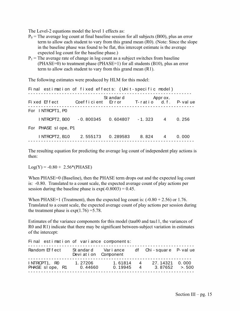
The Level-2 equations model the level 1 effects as: P0 = The average log count at final baseline session for all subjects (B00), plus an error
term to allow each student to vary from this grand mean (R0). (Note: Since the slope in the baseline phase was found to be flat, this intercept estimate is the average expected log count for the baseline phase.)
P1 = The average rate of change in log count as a subject switches from baseline (PHASE=0) to treatment phase (PHASE=1) for all students (B10), plus an error term to allow each student to vary from this grand mean (R1).
The following estimates were produced by HLM for this model: Final estimation of fixed effects: (Unit-specific model) --------------------------------------------------------------- Standard Approx. Fixed Effect Coefficient Error T-ratio d.f. P-value ---------------------------------------------------------------- For INTRCPT1,P0 INTRCPT2,B00 -0.800345 0.604807 -1.323 4 0.256 For PHASE slope,P1 INTRCPT2,B10 2.555173 0.289583 8.824 4 0.000 ---------------------------------------------------------------- The resulting equation for predicting the average log count of independent play actions is then: Log(Y) = -0.80 + 2.56*(PHASE) When PHASE=0 (Baseline), then the PHASE term drops out and the expected log count is: -0.80. Translated to a count scale, the expected average count of play actions per session during the baseline phase is exp(-0.8003) = 0.45. When PHASE=1 (Treatment), then the expected log count is: (-0.80 + 2.56) or 1.76. Translated to a count scale, the expected average count of play actions per session during the treatment phase is exp(1.76) =5.78. Estimates of the variance components for this model (tau00 and tau11, the variances of R0 and R1) indicate that there may be significant between-subject variation in estimates of the intercept: Final estimation of variance components: ---------------------------------------------------------------- Random Effect Standard Variance df Chi-square P-value Deviation Component --------------------------------------------------------------- INTRCPT1, R0 1.27206 1.61814 4 27.14321 0.000 PHASE slope, R1 0.44660 0.19945 4 3.87652 >.500 ----------------------------------------------------------------
Section III – pg. 15

The between-patient variance on intercepts (again, in this case, the average logarithm of the count of play actions per session during the baseline phase) is estimated to be 1.5181 (tau00), which corresponds to a standard deviation of 1.2721. The p-value shown tests the null hypothesis that baseline averages for all subjects are similar. The significant p-value (p<.001) indicates there is a significant amount of variation between subjects on their average baseline frequencies. In other words, the variance is too big to assume it may be due only to sampling error. The between-patient variance in phase slopes (the effect of phase change, or PHASE, on count) is estimated to be 0.1995 (tau11), which corresponds to a standard deviation of 0.4466. The p-value shown for this variance component tests the null hypothesis that the effect of phase change on average log count is similar for all subjects. The p-value here (p>.500) indicates that we cannot detect a significant amount of variation between subjects for this phase effect. We should point out here that due to the small sample size (n=5), there is low power to detect differences among people. But just because the p-value displayed here doesn’t indicate statistically significant variation in phase effects doesn’t mean there isn’t substantial variation in estimates. In fact, if we consider a standard deviation of 0.45 ( 2111tau ) and an estimate of 2.56 (B10) on the log scale, this gives us quite a wide range in estimates when translated back to a count scale, even for a person with an average baseline intercept: B10 1.96(± 2111tau ) = 2.56 1.96(0.45) ± = 2.56 0.88 = (1.68, 3.44) on a log scale, which is ± exp(1.68, 3.44) = (5.37, 31.19) on a count scale Treatment effects are then estimated to range from a factor of 5 to a factor of about 30. Remember that, once exponentiated to a count scale, this is multiplicative effect, meaning that if a student is average on the intercept, as they switch from baseline to treatment phase their expected number of observed play actions is predicted to increase multiplicatively anywhere from 5 to 30 times. The average baseline count was estimated as 0.45 [exp(B00)], so the average treatment phase count may range anywhere from 5.37*(0.45) = 2.42 to 31.19*(0.45) = 14.04. While this variation was not found to be statistically significant, a range of 2.42 to 14.04 on a count scale seems practically important. In order to explore the possibility that certain subject characteristics (Level-2 variables) might account for some of the between-subject variation found, we conducted an exploratory analysis of the potential contributions of Level-2 variables. The section of the output below suggests that COGAGE15 (subjects’ age of cognitive functioning, in months and centered around the approximate median for the sample) and/or KIRKDUM (a dummy variable for Kirk) might help to explain some of the between-subject variance in intercepts and phase effects. (See t-values below.)
Section III – pg. 16

Exploratory Analysis: estimated Level-2 coefficients and their standard errors obtained by regressing EB residuals on Level-2 predictors selected for possible inclusion in subsequent HLM runs ----------------------------------------------------------------Level-1 Coefficient Potential Level-2 Predictors ---------------------------------------------------------------- INTRCPT1,B0 CHRONAGE COGAGE15 KIRKDUM Coefficient 0.616 -0.448 -2.906 Standard Error 1.090 0.066 0.685 t value 0.566 -6.764 -4.244 PHASE,B1 CHRONAGE COGAGE15 KIRKDUM Coefficient -0.216 0.157 1.020 Standard Error 0.383 0.023 0.240 t value -0.566 6.764 4.244 ---------------------------------------------------------------- We investigated these possible Level-2 predictors by entering each into different parts of the model; the results are reported in a later section.
Section III – pg. 17

CONSIDERING THE CONTRIBUTION OF SUBJECT CHARACTERISTICS
(Level-2 Variables in the Prediction Model)
COGAGE15: Exploring subjects’ age of cognitive functioning as a predictor As was suggested by the Exploratory Analysis in the HLM output, certain subject characteristics might be able to explain some of the between-patient variance we found. The strongest suggestion was for COGAGE15, or the age in months of subjects’ cognitive functioning (i.e., had the largest absolute value of t). In the table below, estimates are presented for 3 models run in HLM. The first includes no Level-2 predictors in the model, the next allows COGAGE15 to predict the intercept (or baseline phase average), and the last lets COGAGE15 predict the phase effect. Table III.1. DiCarlo & Reid (2004): Summary Table of HLM Estimates for COGAGE15 on Intercept and Phase. Level-1 Model: log(FREQRND) = P0 + P1*( PHASE) NO L2 Predictors COGAGE15 on Intcpt COGAGE15 on Phase
P0 B00+R0 B00+B01*(COGAGE15)+R0 B00+R0 Level-2 Model P1 B10+R1 B 10+R1 B10+B11*(COGAGE15)+
R1 B00 -0.8003 0.0413 -0.6671 Intcpt B01 -0.3003** B20 2.5552** 2.3974** 2.8239**
Coefficient Estimates
Phase B21 -0.1688 R0 1.2721** 0.1836 1.1376** Variance
Components (SD’s) R1 0.4466 0.0106 0.7627**
Suggestions based on Exploratory Analysis
No other Level-2 variables suggested
COGAGE15 on Intcpt or KIRKDUM on Intcpt or Phase are suggested
No other Level-2 variables suggested
Allowing COGAGE15 to predict the intercept (the model in the center of the table) explains the most variance in both intercepts and phase effects. COGAGE15 significantly predicts the intercept and reduces the between-subject variance in both intercepts and phase effects to almost zero. The resulting equation for predicting the average log count of independent play actions would then be: Log(FREQRND) = P0 + P1*(PHASE) P0 = B00 + B01*(COGAGE15) + R0 P1 = B10 + R1
Section III – pg. 18

And is estimated as: Log(FREQRND) = 0.0413 - 0.3003*(COGAGE15) + 2.3974*(PHASE) Thus, a student close to the sample’s median age of cognitive functioning (COGAGE15=0 when cognitive functioning score = 15 months) in the baseline phase (PHASE=0) is expected to display about 0.04 (B00) log behaviors per session. This translates to an observed count of about 1 play action per session in the baseline phase [exp(0.0413) = 1.0422]. In the treatment phase (PHASE=1), this person is expected to produce about 2.40 (B10) log behaviors per session. This translates to an observed count of about 11 play actions per session in the treatment phase [exp(2.3974) = 10.9945]. Because this is a Poisson model (requiring exponentiation of estimates for translation to a count scale), the model is multiplicative. Therefore the coefficient for COGAGE15’s effect on the intercept of -0.3003 (B01) is not as easily translated or interpreted as the other coefficients. The baseline intercept (average) changes counterintuitively (within context) on a count scale. As COGAGE15 increases, the expected number of play actions observed during baseline decreases and vice versa. A student in this sample with a below-median score on cognitive functioning is predicted to start out higher (with more observed play actions) in the baseline phase than a person of above-median cognitive functioning. After looking at each subject’s cognitive age, we realized that Kirk’s age of cognitive functioning (22 months) was the highest of all 5 subjects, and exceeding the mean cognitive functioning score (17.20) by more than 1.5 standard deviations (SD=3.03), technically qualifying as an outlier. So perhaps it is not actually the cognitive functioning score that makes the difference, but simply being Kirk or not. We explore this possibility next.
KIRKDUM: Exploring whether or not one subject stands out We ran 4 different models in HLM each testing various patterns of Kirk’s possible contribution to the prediction:
1. A simple model with no Level-2 predictors, 2. A model that allows the dummy variable for Kirk to predict Intercept, 3. A model that allows the dummy variable for Kirk to predict Phase, and, 4. A model that allows the dummy variable for Kirk to predict Phase AND Intercept.
When using the untransformed dependent variable (FREQRND) however, we found that HLM had problems estimating some coefficients when Kirk was entered into the model to predict both the baseline intercept (P0) and phase effect (P1), likely due to the necessary use of the Poisson distribution and the high incidence of zeros; therefore we
Section III – pg. 19

also ran these 4 models with a transformed dependent variable. This transformation involves simply adding a small amount (e.g., .01) to each dependent measure taken to overcome the issue of so many zeros but still requires using a Poisson distribution. Except for the most complex model, estimates are quite parallel when using the two versions of the dependent variable. We present both sets of estimates next. Estimates provided by the HLM analyses using both (1) FREQRND and (2) FREQ.01 (i.e., FREQRND + .01) can be found in the summary tables below. Table III.2. DiCarlo & Reid (2004) – Summary Table of HLM Estimates for Poisson model (FML) Level-1 Model: log(L) = P0 + P1*( PHASE)
(1) DV = FREQRND
Model 1 Model 2 Model 3 Model 4 FREQRND NO L2
Predictors KIRKDUM on Intcpt KIRKDUM on Phase KIRKDUM on Phase
AND Intcpt P0 B00+R0 B00+B01*(KIRKDUM)+R0 B00+R0 B00+ B01*(KIRKDUM)+R0Level-2 Model P1 B10+R1 B 10+R1 B10+B11*(KIRKDUM)+ R1 B10+B11*(KIRKDUM)+ R1
B00 -0.8003 -0.2632 -0.5495 -0.2129 Intcpt B01 -1.9615* -32.3652 B20 2.5552** 2.3986** 2.5851** 2.3569**
Coefficient Estimates
Phase B21 -1.4278 30.3828 R0 1.2721** 0.5231* 0.7851** 0.5149* Variance
Components (SDs) R1 0.4466 0.2303 0.4198 0.2225 Likelihood Function -227.1363 -230.9100
Notes SE’s for B01 and B11 are each over 2,000,000.
(2) DV = FREQ+.01
Model 1 Model 2 Model 3 Model 4 FREQ.01 NO L2
Predictors KIRKDUM on Intcpt KIRKDUM on Phase KIRKDUM on Phase
AND Intcpt P0 B00+R0 B00+B01*(KIRKDUM)+R0 B00+R0 B00+ B01*(KIRKDUM)+R0Level-2 Model P1 B10+R1 B 10+R1 B10+B11*(KIRKDUM)+ R1 B10+B11*(KIRKDUM)+ R1
B00 -0.7649 -0.2442 -0.5260 -0.1987 Intcpt B01 -1.9571* -4.4065 B20 2.5225** 2.3817** 2.5649** 2.3439**
Coefficient Estimates Phase
B21 -1.4310 2.4322 R0 1.2336** 0.5151* 0.7687** 0.5077* Variance
Components (SDs) R1 0.4118 0.2228 0.4063 0.2154 Likelihood Function -225.7602 -229.5532
*=p<.05, **=p<.01
Section III – pg. 20

Using either version of the dependent variable, we find that, regardless of Kirk’s place in the model (or not), the expected number of play actions in the baseline phase (B00) is never significantly different from 0 (p>.05 across all models). As well, and again regardless of Kirk’s place in the model, the phase effect (B10) is always significant (p<.05 across all models), indicating a significant difference between baseline and treatment phase averages. The between-subject variance in intercepts (tau00) is always significant (p<.05 across all), though it is reduced when we model KIRKDUM on the intercept. The between-subject variance in phase effects (tau10) is never significant (p>.05 across all), though it is also reduced to some degree when Kirk is allowed to predict the intercept. KIRKDUM (being Kirk or not) does not significantly predict phase effect in either pattern in which it was entered. KIRKDUM does however significantly predict intercept. This is a surprising finding and another example of how statistical findings can challenge the assumptions we make by way of visual inspection. Simply looking at the original graphs, we didn’t detect that Kirk differed so much from the other subjects on the intercept (all had very few observed play actions in the baseline phase). However, output from these analyses show evidence that he does. Knowing whether or not a subject is Kirk (KIRKDUM) significantly predicts a subject’s average count in the baseline phase (B01). As well, when we let KIRKDUM predict the intercept, the between-patient variance on intercepts decreased substantially. When visually inspecting the graphs, we also did expect Kirk to differ from the other subjects on phase effect (he had many fewer observed play actions in the treatment phase than the others). However, output from these analyses suggest that this is not the case statistically. Knowing whether or not a subject is Kirk (KIRKDUM) does not help to predict the change in average count from baseline to treatment phase (B11). When we let KIRKDUM predict phase effect, the between-patient variance on phase effects barely changed.
Section III – pg. 21

ADVANCED TECHNICAL ISSUES
Constraining Random Effects: (BETWEEN-Subject Variation)
An alternative way of exploring whether or not there is significant variation in intercepts or phase effects is to constrain random effects (tau’s) in various patterns and then compare indicators of fit across these models. In constraining tau00, or tau11, or both tau00 AND tau11 to 0 and examining estimates of coefficients and likelihood functions, we can make observations about how much subjects vary from average expectations. Table III.3 summarizes the coefficient estimates, variance components (SD’s), and likelihood functions produced when 4 versions of this analysis were conducted:
2. No constraints on random effects; 3. Tau00 restricted to 0 (intercepts not allowed to vary across subjects); 4. Tau11 restricted to 0 (phase effects not allowed to vary across subjects); 5. Tau00 and Tau11 both restricted to 0
Table III.3. DiCarlo & Reid (2004) – Summary Table of HLM Estimates for Constraining Random Effects (FML) Level-1 Model: log(L) = P0 + P1*( PHASE)
FREQRND
No Constraints
Tau00 = 0 Tau11 = 0
Tau00 = 0 Tau11 = 0
P0 B00+R0 B00 B00 + R0 B00 Level-2 Model P1 B10+R1 B10 + R1 B10 B10
Intcpt B00 -0.8003 -0.4177* -0.5915 -0.4177 Coefficient Estimates Phase B20 2.5552** 2.1747** 2.3392** 2.2378*
R0 1.2721** 0.8387** Variance Components (SD’s) R1 0.4466 0.8160** Likelihood Function -227.1363 -243.2738 -226.0722
Comparing across likelihood functions, we can see that when we restrict Tau00 to 0 (not allowing intercepts to vary across subjects) the model doesn’t fit as well (LF = -243.2738) as when intercepts are allowed to vary in the unconstrained model (LF = -227.1363). It seems then that between-subject variation in intercepts should be considered in the model. However, omitting Tau11 (not allowing phase effects to vary) doesn’t seem to affect fit at all (LF = -226.0722). This means that it is reasonable to constrain the phase effect so that it is the same for all subjects.3 3 No likelihood function would print on the output for the model with both the intercept and the slope constrained.
Section III – pg. 22

Looking at Heterogeneity of Level-1 Variance across Phases: (WITHIN-Subject
Variation) One hypothesis for why significant between-subject variance in phase effects could not be detected is that it is hidden by the within-subject variation in the treatment phase. A visual inspection of the original graphs suggested that there may be greater within-subject variation in observations made during the treatment phase than in those made during the baseline phase. If data varies greatly within-subjects during the treatment phase, then averages taken are less accurate representations of what is happening in the treatment phase and estimates of change from baseline phase average to treatment phase average (phase effect) may not be well-detected. HLM 6 will examine such heterogeneity of Level-1 variance (sigma-squared) between phases as part of its Estimation Setting options, however the program will not allow this option to be selected for Poisson models. So although the technically correct way to analyze this model is to use a Poisson distribution, we performed some transformations on the dependent variable to allow us to use a linear model instead, permitting somewhat easier interpretation, helping to overcome the problems we encountered due to the high incidence of zero frequencies, and permitting a test of the heterogeneity of Level-1 (within-subject) variance across phases. Two transformations typically used in this situation, both of which allow us to use a linear rather than a Poisson distribution, include: (1) taking the square root of the dependent variable (and then squaring subsequent estimates); and, (2) adding a small amount (0.01) to the original rounded dependent variable and then taking the log of that sum (exponentiating estimates as we did with the Poisson). With each transformed outcome variable, a simple model with B00 (baseline intercept) and B10 (treatment effect) was run. Estimates are displayed in Table III.4. The final row of the table displays the results of the test of heterogeneity of Level-1 variances across phases.
Section III – pg. 23

Table III.4. DiCarlo & Reid (2004): Comparison of Transformed Dependent Variables. Transformed DV (1) FREQSQRT (2) LNFREQ01 Transformation Computation FREQRND LN(FREQRND + 0.01)
Level-1 Equation FREQSQRT = P0 + P1*(PHASE) LNFREQ01 = P0 + P1*(PHASE)
Level-2 Equations P0 = B00 + R0 P1 = B10 + R1
P0 = B00 + R0 P1 = B10 + R1
Coefficient Estimates
B00 = 0.3511 B10 = 2.0319*
B00 = -3.4627** B10 = 4.4720**
Variance Components (SD’S)
R0 = 0.0407 R1 = 0.9037**
R0 = 0.7453 R1 = 0.8731
Average Baseline (on Freq scale) 0.35112 = 0.1233 exp(-3.4627) = 0.0313
Average Treatment Phase (on Freq Scale)
0.1233 + 2.03192
= 0.1233 + 4.1286 = 4.2519
0.0313*exp(4.4720) = 0.0313*87.5316 = 2.7397
Deviance 256.1401 426.2514
Summary of Model Fit (Phase)
1. Homogeneous Sigma^2 = 256.1401 2. Heterogeneous Sigma^2 = 250.4821 Chi-square (model 1 vs. model 2) = 5.6580*
1. Homogeneous Sigma^2 = 426.2514 2. Heterogeneous Sigma^2 = 424.8636 Chi-square (model 1 vs. model 2) = 1.3875
The results on the log scale are very comparable to the Poisson model we fit in a previous section, and the analysis here corroborates those results. Once again, our assumptions via visual inspection are challenged by statistical findings. Although a visual examination of the data seemed to suggest greater heterogeneity of Level-1 data (within-subject variation) in the treatment phase than in the baseline phase, examining this statistically on a log scale shows that this is not actually the case.
Section III – pg. 24

SECTION IV. Two-Phase Designs, Outcome = Proportion A third published study was selected to extend the illustration of the analysis of data from a two-phase (A-B) study with a categorical dependent variable:
Hunt, P., Soto, G., Maier, J., Doering, K. (2003). Collaborative teaming to
support students at risk and students with severe disabilities in general education classrooms. Exceptional Children, 69(3), 315-332.
In this study, researchers observed the academic and social participation behavior of six elementary school students in general education inclusion classes at two schools. Three of these students had diagnosed severe disabilities. The other three students were identified as academically-at-risk. Observations took place in each classroom, over several months. The target behavior of interest for this analysis is focus student initiation of interactions with the teacher or other students. Each observation period was segregated into 60 intervals or trials. For each trial, the researcher noted whether or not the focus student had initiated a social interaction with the teacher or other students at least once. The percentage of trials where the student did initiate interactions was computed and recorded as the end measure for each day of observation. The dependent variable in this dataset is then a proportion (successful trials out of total trials), which must be accommodated in the analyses and in subsequent interpretation. Such accommodations are discussed below. There were two phases in the study. For the first three to eight observation days (depending on the subject), students were observed without intervention, in the baseline phase. After this baseline phase, a collaborative teaming process was implemented whereby teachers, aides, and parents collaborated to plan and implement individualized support plans including academic adaptations and communications and social supports for each child in the study. The remaining observations were made during the implementation of this treatment. Again, observations should be coded by phase so that proportion variations within and across the two phases can be examined. Line graphs, scanned and pasted from the original publication, plotting the percentage of intervals of focus student-initiated interactions to the teachers or other students (Y) by days of observation (X) for each subject, are presented below. For each, the data points to the left of the vertical line indicate observations taken during the baseline phase and the points to the right of the vertical line indicate observations taken during the treatment phase.
Section IV – pg. 1

Figure IV.1. Hunt, Soto, Maier & Doering (2003). Percentage of intervals of focus student-initiated interactions to the teachers or other students by day, and phase, for subjects 1-6.
Because the dependent variable is a proportion from a fixed number of binary (0, 1) observations, we chose to use a binomial distribution when analyzing the data (instead of a normal distribution). The binomial is used to model the number of events that took place where the total possible number of events is known. In this example, we know that for each day of observation, a total of 60 trials were observed. A 100% on the dependent measure would indicate that in 60 out of 60 trials the focus student was observed initiating an interaction. A measure of 50% would indicate the student initiated interactions during 30 of the 60 trials on that day. Additional (Level-2) data were available on subjects’ gender, type of disability (physical, speech/language, social), at-risk status, race/ethnicity and class location. At the time this study was published, these variables had not been explored as potential explanatory factors in the variation of initiated interactions.
Section IV – pg. 2

Multilevel modeling (using the HLM software) was again utilized to: (1) model the overall change in the proportion of initiated interactions for each student, (2) combine results of all students in the study so that we may examine trends across the study and between students, and, (3) model the change in proportion of initiated interactions between phases. HLM allowed us to examine the significance of student characteristics (e.g., gender, race/ethnicity, disability, etc) that may account for variations among intercepts and slopes. Does this treatment work differently for different types of students? In order to perform such analyses and to simplify interpretation, several variables had to be recoded and/or created anew. Level-1 variable recodes and calculations include:
The number of binomial trials was entered as 60 for each observation, to indicate the total number of possible trials on each day. (TRIALS)
The dependent variable was translated from a percent (out of 100) to a frequency, to indicate the number of successful trials for each day. (FREQ60)
Phase was coded as 0 for baseline and 1 for treatment. (PHASE) Day of observation was recentered so that 0 represented the observation right before the
phase change. (DAYSC) A variable for the day-by-phase interaction was computed by multiplying the two
previous variables. (DAYCxPHA) Level-2 variables also needed to be created from the text of the article. All were categorical:
Gender was coded as a 0 for Male and a 1 for Female. (FEMALE) Disability was coded as a 0 for “severely disabled” and a 1 for “academically-at-risk”.
(ATRISK) Physical disability was coded as a 0 for no physical disability and a 1 if the child had a
documented physical disability. (PHYSDIS) Speech/language disability was coded as a 0 for no speech/language disability and a 1 if
the child had a documented speech/language disability. (LANGDIS) Social disability was coded as a 0 for no social difficulties and a 1 if the child had
documented social difficulties. (SOCPROB) Race/Ethnicity was coded into two separate variables:
o BLACK was coded as a 0 for students who were not indicated as African American and a 1 for students who were indicated as being African American.
o LATINO was coded as a 0 for students who were not indicated as Latino or Hispanic and a 1 for students who were indicated as being Latino or Hispanic.
Class was coded as a 0 if the student was in Class A and a 1 if the student was in Class B. (CLASSB)
An interaction term was created to check for the crossover effect between class location (A or B) and disability (disabled or academically at-risk) by multiplying CLASSB and ATRISK, resulting in a binary (0,1) variable. (CLSxRISK)
Therefore, a 0 on all Level-1 variables (days, phase, days-by-phase interaction) denotes the final baseline session. Intercepts for the computed models are predicted proportions at the phase change. The full model (without any Level-2 predictors) is then:
Section IV – pg. 3

Level-1: Log[P/(1-P)] = P0 + P1*(DAYSC) + P2*(PHASE) + P3*(DAYCxPHA)
Level-2: P0 = B00 + R0 P1 = B10 + R1 P2 = B20 + R2 P3 = B30 + R3
Details about how to create and/or transform the Level-1 and Level-2 variables are described below. Note about using the Binomial distribution: Whereas the Poisson is used to model the frequency of some event in a given period of time (i.e., a rate as in Dicarlo & Reid (2004)), the Binomial is used to model the frequency of some binomial (yes, no) event out of a total known number of possible binary trials (i.e., a proportion). For both types of distributions, observations are assumed to be independent and identical. In other words, the outcome of one observation is not expected to affect the outcome of another observation and the probability of success on a trial is the same for all trials. Unlike normal distributions in which the variance is a completely separate parameter from the mean, in Binomial and Poisson distributions the variance is a function of the mean. For the Poisson distribution, the mean and the variance are equal. As the mean increases, so does the variance. Counts tend to vary more when their average value is higher (Agresti, 1996). For the Binomial, the variance is largest when the proportion is .5. These relations between the mean and variance of the distributions are also sometimes violated. When count data (including both rates and proportions) exhibit greater variability than would be expected by the Poisson or Binomial models, the result is usually overdispersion. Overdispersion can be caused by statistical dependence or heterogeneity among subjects (Agresti, 1996, 2002). We can accommodate for this in the analyses by selecting an option in HLM6 (Raudenbush & Bryk, 2002; Raudenbush et al, 2004). This accommodation is demonstrated in the following illustration.
Section IV – pg. 4
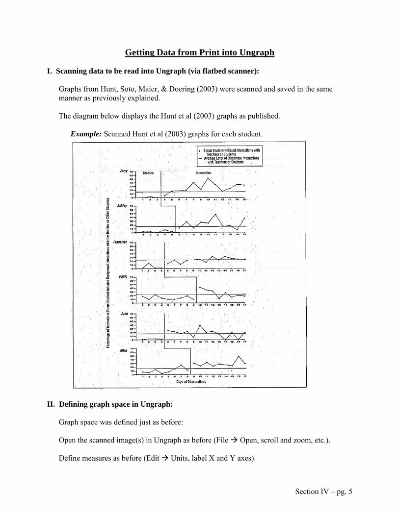
Getting Data from Print into Ungraph
I. Scanning data to be read into Ungraph (via flatbed scanner): Graphs from Hunt, Soto, Maier, & Doering (2003) were scanned and saved in the same manner as previously explained. The diagram below displays the Hunt et al (2003) graphs as published. Example: Scanned Hunt et al (2003) graphs for each student.
II. Defining graph space in Ungraph:
Graph space was defined just as before: Open the scanned image(s) in Ungraph as before (File Open, scroll and zoom, etc.). Define measures as before (Edit Units, label X and Y axes).
Section IV – pg. 5

Define the Coordinate System as before (Edit Define Coordinate System, etc.).
III. Reading in & exporting data:
Data from Hunt et al (2003) was read in and exported just as was data from Dicarlo & Reid (2004) (as a scatterplot). Read in data from graph just as before (Digitize New Scatter). Export Data just as before. (Select Data Export) saving each subject’s data separately.
Repeat each of these steps in sections II and III (from Defining Graph Space to Reading in
and Exporting Data) for each Level-1 (subject) graph available.
Save each of the Level-1 files as separate .txt files, labeled by case name or ID number.
Section IV – pg. 6
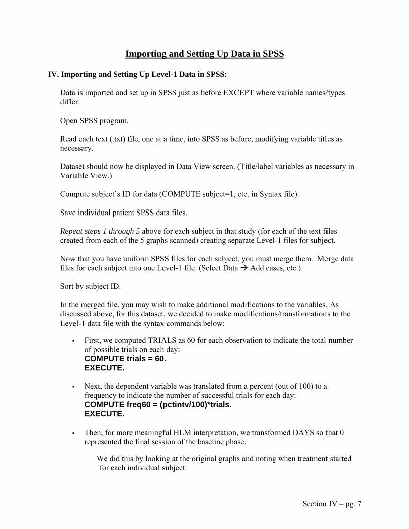
Importing and Setting Up Data in SPSS
IV. Importing and Setting Up Level-1 Data in SPSS:
Data is imported and set up in SPSS just as before EXCEPT where variable names/types differ:
Open SPSS program. Read each text (.txt) file, one at a time, into SPSS as before, modifying variable titles as necessary. Dataset should now be displayed in Data View screen. (Title/label variables as necessary in Variable View.) Compute subject’s ID for data (COMPUTE subject=1, etc. in Syntax file). Save individual patient SPSS data files. Repeat steps 1 through 5 above for each subject in that study (for each of the text files created from each of the 5 graphs scanned) creating separate Level-1 files for subject. Now that you have uniform SPSS files for each subject, you must merge them. Merge data files for each subject into one Level-1 file. (Select Data Add cases, etc.) Sort by subject ID. In the merged file, you may wish to make additional modifications to the variables. As discussed above, for this dataset, we decided to make modifications/transformations to the Level-1 data file with the syntax commands below:
First, we computed TRIALS as 60 for each observation to indicate the total number of possible trials on each day: COMPUTE trials = 60. EXECUTE.
Next, the dependent variable was translated from a percent (out of 100) to a frequency to indicate the number of successful trials for each day: COMPUTE freq60 = (pctintv/100)*trials. EXECUTE.
Then, for more meaningful HLM interpretation, we transformed DAYS so that 0
represented the final session of the baseline phase.
We did this by looking at the original graphs and noting when treatment started for each individual subject.
Section IV – pg. 7

We then wrote and ran the following syntax command (the value subtracted from each subject’s DAYS is the last observation day before the vertical line in the graph, indicating the phase change): If (subject=1) daysc = days - 3. If (subject=2) daysc = days - 5. If (subject=3) daysc = days - 4. If (subject=4) daysc = days - 9. If (subject=5) daysc = days - 4. If (subject=6) daysc = days - 8. EXECUTE.
We created a variable to indicate in which PHASE (baseline or treatment) a
measurement was taken by running the following syntax: COMPUTE phase = 0. If (daysc>0) phase = 1. EXECUTE.
Finally, we created an interaction variable so that we could later examine whether or
not there were any significant interactions between days (DAYSC) and phase (i.e., did slopes differ by phase): COMPUTE daycXpha = daysc*phase. EXECUTE.
12. After making all modifications and making sure to sort by subject ID, re-save complete Level-1 file and close.
VI. Entering and Setting Up Level-2 Data in SPSS
Create SPSS file including any Level-2 data (subject characteristics) available, as before.
In this study, data could be gathered from the text on each subject’s gender, disability
or at-risk status, race/ethnicity, class location, and type of disabilities: A dummy variable was created for each gender, disability/at-risk status, and
classroom location: FEMALE = 0 for males and 1 for females ATRISK = 0 for “severely disabled” and 1 for “academically at-risk” CLASSB = 0 for students in Class A and 1 for students in Class B
Additional dummy variables were created for each type of disability indicated: PHYSDIS = 0 for no physical disability and 1 if the child had a documented
physical disability LANGDIS = 0 for no speech/language disability and 1 if the child had a
documented speech/language disability SOCPROB = 0 for no social difficulties and 1 if the child had documented
social difficulties A set of 2 dummy variables were created to indicate race/ethnicity:
BLACK = 0 for students who were not indicated as being African American and 1 for students who were indicated as being African American
Section IV – pg. 8

LATINO = 0 for students who were not indicated as being Latino or Hispanic and 1 for students who were indicated as being Latino or Hispanic
Create or transform any additional Level-2 variables as necessary.
An interaction term (CLSXRISK) was created to check for the crossover effect
between class location (A or B) and disability status (being disabled or academically at-risk):
COMPUTE clsXrisk = classb*atrisk. EXECUTE.
Our Level-2 data file then was left with 10 working variables: SUBJECT, FEMALE,
ATRISK, CLASSB, PHYSDIS, LANGDIS, SOCPROB, BLACK, LATINO, and CLSXRISK.
Section IV – pg. 9

Setting Up and Running Models in HLM (Poisson)
VI. Setting up MDM file in HLM6:
The MDM file for the Hunt et al (2003) data was set up just as the preceding MDMs.
Open HLM program. (making sure all related SPSS files are saved and closed) Select File Make new MDM file Stat package input On next window, leave HLM2 bubble selected and click OK. Label MDM file (entering file name ending in .mdm, and indicate Input File Type as SPSS/Windows) Specify structure of data (again, this data is nested within subjects so under Nesting of input data we selected measures within persons) Specify Level-1 data (browsing and opening Level-1 file and indicating subject ID and all other relevant Level-1 variables – FREQ60, TRIALS, PHASE, DAYSC, DAYCxPHA). Specify Level-2 data (browsing and opening Level-2 file and indicating subject ID and all other relevant Level-2 variables – FEMALE, ATRISK, CLASSB, PHYSDIS, LANGDIS, SOCPROB, BLACK, LATINO, CLSXRISK). Save Response File (clicking on Save mdmt file, naming and saving file) Make MDM (clicking on Make MDM) Check Stats (clicking Check Stats) Click on Done.
VII. Setting up the model:
Because the dependent variable in this dataset is a proportion, there are new differences in how the HLM analyses were set up. With MDM file (just created) open in HLM,
Choose outcome variable:
With Level-1 menu selected, click on FREQ60 and then Outcome variable to specify it as the outcome measure.
Identify which Level-1 predictor variables you want in the model.
Section IV – pg. 10

Click on DAYSC and then add variable uncentered. Repeat for PHASE and DAYCxPHA.
Activate Error terms: Make sure to activate relevant error terms (depending on model) in each Level-2 equation by clicking on the error terms individually ( ). ,..., 21 rr
In this case, we activated all Level-2 error terms.
Modify model set up to accommodate dependent variable type:
Because the dependent variable in this study is a proportion (successful trials out of total trials), we must indicate to HLM that this variable has a Binomial distribution.
Select Basic Settings and choose Binomial distribution (number of trials) under
Distribution of Outcome Variable From the drop-down menu to the right of the binomial selection, highlight and
choose TRIALS as the indicator of number of trials.
Title output and graphing files, while you are in Basic Settings:
Fill in Title (this is the title that will appear printed at the top of the output text file). Fill in Output File Name and location (this is the name and location where the output
file will be saved); and Graph File Name and location (this is the name and location where the graph file will be saved).
Click OK to exit this screen.
Select Overdispersion option, while you are in Basic Settings:
Check the box labeled Overdispersion to allow accommodation for possible overdispersion discussed above. (Output will be examined to check that this accommodation is necessary. As well, the final model will be run both with and without this option selection to check that estimates of fixed effects remain stable.)
Section IV – pg. 11

Example: Hunt et al (2003) – Setting up models in HLM
Exploratory Analysis: Select Other Settings Exploratory Analysis (Level-2)
Click on each Level-2 variable that you want to include in the exploratory analysis
and click add. (In this case, we selected FEMALE, ATRISK, CLASSB, PHYSDIS, LANGDIS, SOCPROB, BLACK, LATINO, and CLSXRISK.)
Click on Return to Model Mode at top right of screen.
Run the analysis
At the top of the screen, click on Run Analysis.
On the pop-up screen, click on Run model shown.
View Output:
Select File View Output
Section IV – pg. 12
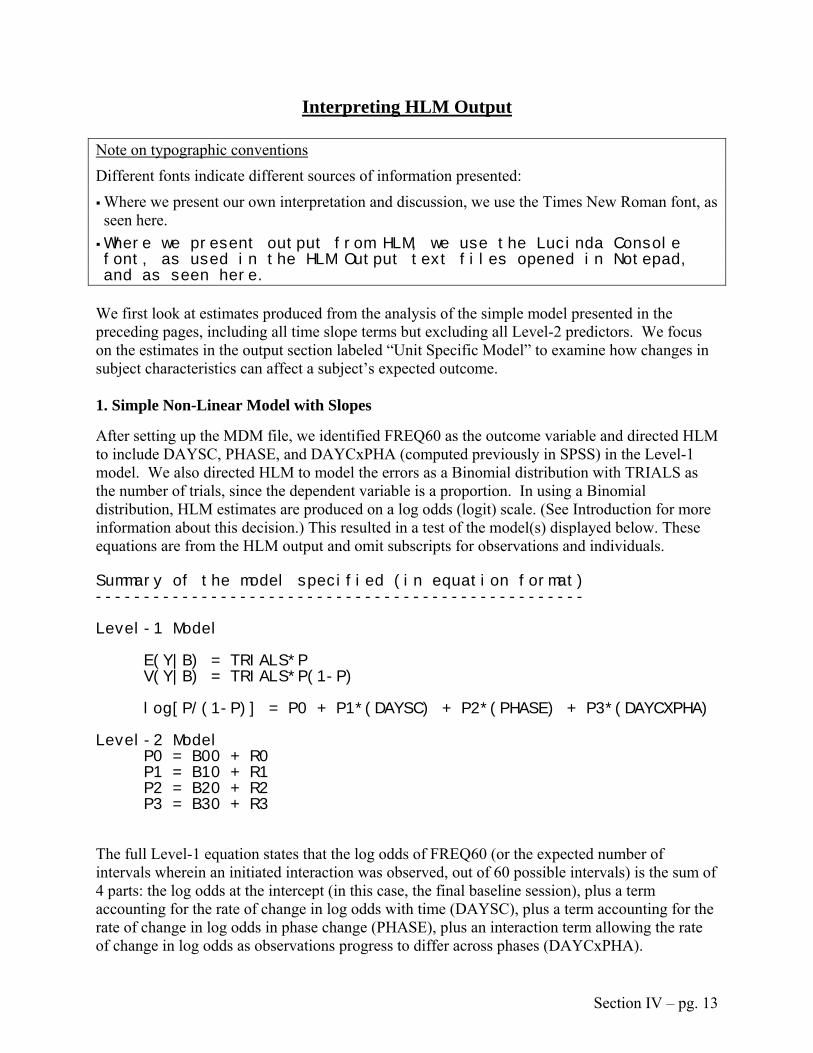
Interpreting HLM Output
Note on typographic conventions
Different fonts indicate different sources of information presented:
Where we present our own interpretation and discussion, we use the Times New Roman font, as seen here.
Where we present output from HLM, we use the Lucinda Console font, as used in the HLM Output text files opened in Notepad, and as seen here.
We first look at estimates produced from the analysis of the simple model presented in the preceding pages, including all time slope terms but excluding all Level-2 predictors. We focus on the estimates in the output section labeled “Unit Specific Model” to examine how changes in subject characteristics can affect a subject’s expected outcome. 1. Simple Non-Linear Model with Slopes After setting up the MDM file, we identified FREQ60 as the outcome variable and directed HLM to include DAYSC, PHASE, and DAYCxPHA (computed previously in SPSS) in the Level-1 model. We also directed HLM to model the errors as a Binomial distribution with TRIALS as the number of trials, since the dependent variable is a proportion. In using a Binomial distribution, HLM estimates are produced on a log odds (logit) scale. (See Introduction for more information about this decision.) This resulted in a test of the model(s) displayed below. These equations are from the HLM output and omit subscripts for observations and individuals. Summary of the model specified (in equation format) --------------------------------------------------- Level-1 Model E(Y|B) = TRIALS*P V(Y|B) = TRIALS*P(1-P) log[P/(1-P)] = P0 + P1*(DAYSC) + P2*(PHASE) + P3*(DAYCXPHA) Level-2 Model P0 = B00 + R0 P1 = B10 + R1 P2 = B20 + R2 P3 = B30 + R3 The full Level-1 equation states that the log odds of FREQ60 (or the expected number of intervals wherein an initiated interaction was observed, out of 60 possible intervals) is the sum of 4 parts: the log odds at the intercept (in this case, the final baseline session), plus a term accounting for the rate of change in log odds with time (DAYSC), plus a term accounting for the rate of change in log odds in phase change (PHASE), plus an interaction term allowing the rate of change in log odds as observations progress to differ across phases (DAYCxPHA).
Section IV – pg. 13

This full model does not include any Level-2 predictors (student characteristics). The Level-2 equations model the level 1 intercepts and slopes as:
P0 = The average log odds at final baseline session for all subjects (B00), plus an error term to allow each student to vary from this grand mean (R0).
P1 = The average rate of change in log odds per day of observation (DAYSC) during the baseline phase (B10), plus an error term to allow each student to vary from this grand mean effect (R1). (Remember that DAYSC was recoded so that 0=last baseline observation.)
P2 = The average rate of change in log odds as a subject switches from baseline to treatment phase (PHASE) for all students (B20), plus an error term to allow each student to vary from this grand mean (R2).
P3 = The average change in day-of-observation effect (i.e., time slope) as a subject switches from baseline to treatment phase for all students (B30), plus an error term to allow each student to vary from this grand mean (R3).
The following estimates were produced by HLM for this model: Final estimation of fixed effects: (Unit-specific model) ---------------------------------------------------------------- Standard Approx. Fixed Effect Coefficient Error T-ratio d.f. P-value ---------------------------------------------------------------- For INTRCPT1, P0 INTRCPT2, B00 -2.839034 0.463513 -6.125 5 0.000 For DAYSC slope, P1 INTRCPT2, B10 0.005931 0.085128 0.070 5 0.948 For PHASE slope, P2 INTRCPT2, B20 1.775542 0.437250 4.061 5 0.013 For DAYCXPHA slope, P3 INTRCPT2, B30 -0.017581 0.086423 -0.203 5 0.847 ---------------------------------------------------------------- When DAYSC=0 and PHASE=0 and DAYCXPHA=0 (i.e., the final baseline observation), the overall average log odds ratio for all students is –2.8390 (B00). [exp(-2.8390) = 0.0585; 0.0585/1.0585 = 0.0553] The expected probability of observing a student initiating an interaction during the final baseline observation is 0.05. The average rate of change in log odds per day of observation is -0.0059 (B10). This increase is not significant as the p-value for B10 is greater than .05. Therefore, we can conclude that the baseline trend is flat, not changing over time (days). The average rate of change in log odds as a student switches from baseline (PHASE=0) to treatment phase (PHASE=1) is 1.7755 (B20). This phase effect is significant as the p-value for B20 is less than .05 (or even .01). [exp(-2.8390 + 1.7755) = exp(-1.0635) = 0.3452;
Section IV – pg. 14
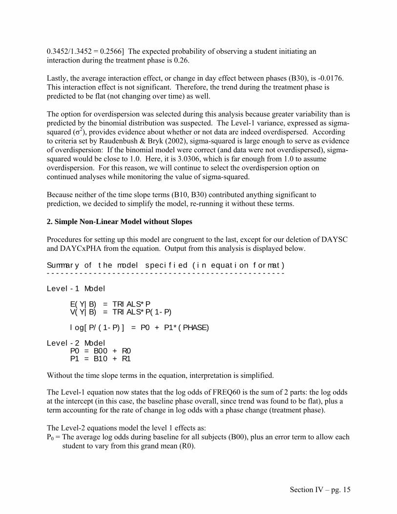
0.3452/1.3452 = 0.2566] The expected probability of observing a student initiating an interaction during the treatment phase is 0.26. Lastly, the average interaction effect, or change in day effect between phases (B30), is -0.0176. This interaction effect is not significant. Therefore, the trend during the treatment phase is predicted to be flat (not changing over time) as well. The option for overdispersion was selected during this analysis because greater variability than is predicted by the binomial distribution was suspected. The Level-1 variance, expressed as sigma-squared (σ2), provides evidence about whether or not data are indeed overdispersed. According to criteria set by Raudenbush & Bryk (2002), sigma-squared is large enough to serve as evidence of overdispersion: If the binomial model were correct (and data were not overdispersed), sigma-squared would be close to 1.0. Here, it is 3.0306, which is far enough from 1.0 to assume overdispersion. For this reason, we will continue to select the overdispersion option on continued analyses while monitoring the value of sigma-squared. Because neither of the time slope terms (B10, B30) contributed anything significant to prediction, we decided to simplify the model, re-running it without these terms. 2. Simple Non-Linear Model without Slopes Procedures for setting up this model are congruent to the last, except for our deletion of DAYSC and DAYCxPHA from the equation. Output from this analysis is displayed below. Summary of the model specified (in equation format) --------------------------------------------------- Level-1 Model E(Y|B) = TRIALS*P V(Y|B) = TRIALS*P(1-P) log[P/(1-P)] = P0 + P1*(PHASE) Level-2 Model P0 = B00 + R0 P1 = B10 + R1 Without the time slope terms in the equation, interpretation is simplified. The Level-1 equation now states that the log odds of FREQ60 is the sum of 2 parts: the log odds at the intercept (in this case, the baseline phase overall, since trend was found to be flat), plus a term accounting for the rate of change in log odds with a phase change (treatment phase). The Level-2 equations model the level 1 effects as: P0 = The average log odds during baseline for all subjects (B00), plus an error term to allow each
student to vary from this grand mean (R0).
Section IV – pg. 15

P1 = The average rate of change in log odds as a subject switches from baseline (PHASE=0) to treatment phase (PHASE=1) for all students (B10), plus an error term to allow each student to vary from this grand mean (R1).
The following estimates were produced by HLM for this model: Final estimation of fixed effects: (Unit-specific model) ---------------------------------------------------------------- Standard Approx. Fixed Effect Coefficient Error T-ratio d.f. P-value ---------------------------------------------------------------- For INTRCPT1,P0 INTRCPT2,B00 -2.860854 0.393467 -7.271 5 0.000 For PHASE slope,P1 INTRCPT2,B10 1.744330 0.350792 4.973 5 0.002 ---------------------------------------------------------------- When PHASE=0 (i.e., the baseline phase), the overall average log odds of initiating an interaction for all students is -2.8609 (B00). [exp(-2.8609) = 0.0572; 0.0572/1.0572 = 0.0541] The expected probability of observing a student initiating an interaction during the baseline phase is 0.05. The average rate of change in log odds as a student switches from baseline (PHASE=0) to treatment (PHASE=1) is 1.7443 (B10). This phase effect is significant as the p-value for B10 is less than .05. [exp(-2.8609 + 1.7443) = exp(-1.1166) = 0.3274; 0.3274/1.3274 = 0.2466] The expected probability of observing a student initiating an interaction during the treatment phase is the 0.25. Estimates of the variance components for this model (tau00 and tau11) indicate that there may be significant between-subject variation in estimates of the intercept and phase effect: Final estimation of variance components: ---------------------------------------------------------------- Random Effect Standard Variance df Chi-square P-value Deviation Component ---------------------------------------------------------------- INTRCPT1,R0 0.82576 0.68188 5 36.13696 0.000 PHASE slope,R1 0.67666 0.45787 5 18.74659 0.003 Level-1,E 1.81836 3.30643 ---------------------------------------------------------------- The between-subject variance on intercepts is estimated to be 0.6819 (tau00), which corresponds to a standard deviation of 0.8258. The p-value shown tests the null hypothesis that baseline averages for all subjects are similar. The significant p-value indicates there is a significant amount of variation between subjects on their average baseline frequencies. In other words, the variance is too big to assume it may be due only to sampling error.
Section IV – pg. 16

The between-subject variance in phase effect (the effect of phase change, or PHASE, on probability) is estimated to be 0.4579 (tau11), which corresponds to a standard deviation of 0.6767. The p-value shown for this variance component tests the null hypothesis that the effect of phase change on average probability is similar for all subjects. The significant p-value here indicates there is also a significant amount of variation between subjects on the effect of treatment. Once again, the value of sigma-squared (3.3064) suggests that accommodating for overdispersion is appropriate here. In order to explore the possibility that certain subject characteristics (Level-2 variables) might account for some of the between-subject variation found (i.e., that treatment might work different for different types of students), we conducted an exploratory analysis of the potential contributions of Level-2 variables. The section of output below suggests that CLSxRISK (the interaction between classroom and disability/at-risk status) might help to explain some of the between-subject variance in intercepts and phase effects (see associated t-values below). It should be noted that the effect of this created variable is speculative as there is no available evidence that the 2 subjects who are academically at-risk in Class B (and then stand out, as 1’s, on this created variable) should differ from the others. The variable was created and tested after a visual analysis of the graphs suggested that subjects 4 and 6 seem to show an unusual pattern in baseline and treatment proportions and that they were the only students in Class B labeled as academically at-risk rather than disabled.
Section IV – pg. 17

Exploratory Analysis: estimated Level-2 coefficients and their standard errors obtained by regressing EB residuals on Level-2 predictors selected for possible inclusion in subsequent HLM runs ---------------------------------------------------------------- Level-1 Coefficient Potential Level-2 Predictors ---------------------------------------------------------------- FEMALE ATRISK CLASSB PHYSDIS LANGDIS SOCPROB INTRCPT1,B0 Coefficient 0.246 0.879 0.552 -0.922 -0.922 -0.938 Standard Error 0.692 0.496 0.646 0.530 0.530 0.468 t value 0.355 1.773 0.854 -1.740 -1.740 -2.005 BLACK LATINO CLSXRISK INTRCPT1 slope,B0 Coefficient -0.552 -0.746 1.298 Standard Error 0.646 0.595 0.269 t value -0.854 -1.253 4.823 FEMALE ATRISK CLASSB PHYSDIS LANGDIS SOCPROB PHASE,B1 Coefficient -0.187 -0.713 -0.475 0.749 0.749 0.742 Standard Error 0.560 0.400 0.516 0.427 0.427 0.386 t value -0.334 -1.784 -0.920 1.755 1.755 1.923 BLACK LATINO CLSXRISK PHASE slope,B1 Coefficient 0.475 0.581 -1.056 Standard Error 0.516 0.488 0.209 t value 0.920 1.191 -5.044 ----------------------------------------------------------------
Section IV – pg. 18

3. CLSxRISK predicts Intercept and Phase Effects We investigated CLSxRISK as a possible Level-2 predictor by entering each into the model for the intercept (P0) and the phase effect (P1). Summary of the model specified (in equation format) --------------------------------------------------- Level-1 Model E(Y|B) = TRIALS*P V(Y|B) = TRIALS*P(1-P) log[P/(1-P)] = P0 + P1*(PHASE) Level-2 Model P0 = B00 + B01*(CLSXRISK) + R0 P1 = B10 + B11*(CLSXRISK) + R1 Adding CLSxRISK to the model at Level-2 does not change the Level-1 equation, on its own. The Level-1 equation still states that the log odds of FREQ60 is the sum of 2 parts: the log odds at the intercept (in this case, the baseline phase overall, since trend was found to be flat), plus a term accounting for the rate of change in log odds with a phase change (treatment phase). The Level-2 equations, however, do change: P0 = The average log odds during baseline for all subjects (B00), plus a term allowing for the
effect of being academically at-risk in Class B (B01), plus an error term to allow each student to vary from the mean effect (R0).
P1 = The average rate of change in log odds as a subject switches from baseline (PHASE=0) to treatment phase (PHASE=1) for all students (B10), plus a term allowing for the effect of being academically at-risk in Class B (B11), plus an error term to allow each student to vary from the mean effect (R1).
Final estimation of fixed effects: (Unit-specific model) ---------------------------------------------------------------- Standard Approx. Fixed Effect Coefficient Error T-ratio d.f. P-value ---------------------------------------------------------------- For INTRCPT1, P0 INTRCPT2, B00 -3.529487 0.361212 -9.771 4 0.000 CLSXRISK, B01 1.615009 0.409151 3.947 4 0.027 For PHASE slope, P1 INTRCPT2, B10 2.327101 0.387693 6.002 4 0.000 CLSXRISK, B11 -1.355424 0.480548 -2.821 4 0.049 ----------------------------------------------------------------
Section IV – pg. 19

When PHASE=0 (i.e., the baseline phase) and CLSxRISK=0 (i.e., not subjects 4 or 6), the overall average log odds of initiating an interaction is estimated to be -3.5295 (B00). [exp(-3.5295) = 0.0293; 0.0293/1.0293 = 0.0285] The expected probability of observing a student, other than subjects 4 and 6, initiating an interaction during the baseline phase is 0.03. Being subject 4 or 6 (CLSxRISK=1), changes the log odds of initiating an interaction during baseline by 1.6151. Therefore, the average log odds of initiating an interaction in the baseline for these 2 subjects is -3.5295 + 1.6151 = -1.9144. [exp(-1.9144) = 0.1474; 0.1474/1.1474 = 0.1285] The expected probability of observing student 4 or 6 (at-risk students in Class B) initiating an interaction during baseline is 0.13. The average rate of change in log odds as a student, other than 4 or 6, switches from baseline (PHASE=0) to treatment (PHASE=1) is 2.3271 (B10). This phase effect is significant as the p-value for B10 is less than .05. [exp(-3.5295 + 2.3271) = exp(-1.2024) = 0.3005; 0.3005/1.3005 = 0.2310] The expected probability of observing a student, other than 4 or 6, initiating an interaction during the treatment phase is the 0.23. Being subject 4 or 6 (CLSxRISK=1), changes the log odds effect of treatment on initiating an interaction by -1.3554. Therefore, the average log odds of initiating an interaction in the treatment phase for these 2 subjects is -3.5295 + 1.6151 + 2.3271 -1.3554 = - 0.9427. [exp(-0.9427) = 0.3896; 0.3896/1.3896 = 0.2804] The expected probability of observing student 4 or 6 (at-risk students in Class B) initiating an interaction during the treatment phase is 0.28. Estimates of the variance components for this model (tau00 and tau11) indicate that, once we include CLSxRISK in the model, there is no significant between-subject variation in estimates of the intercept and phase effect left. Final estimation of variance components: ---------------------------------------------------------------- Random Effect Standard Variance df Chi-square P-value Deviation Component ---------------------------------------------------------------- INTRCPT1,R0 0.12068 0.01456 4 2.82682 >.500 PHASE slope,R1 0.25877 0.06696 4 3.60923 >.500 Level-1,E 1.84119 3.38999 ---------------------------------------------------------------- This seems to be a well-fitting model with a better indication of model fit (LF=-197.5778) and the least amount of residual variation in estimates. Table IV.1 summarizes the estimates produced by all four models run.
Section IV – pg. 20

Table IV.1. Hunt, Soto, Maier, & Doering (2003): HLM Estimates, DV = Freq60 (calc’d from [(% of intervals/100)*60 intervals]) Run as Binomial Distribution with Trials = TRIALS(60) and Restricted ML estimation E(Y|B) = TRIALS*P FULL Level-1 Model: log[P/(1-P)] = P0 + P1*(DAYSC) + P2*(PHASE) + P3*(DAYCxPHA) SIMPLIFIED Level-1 Model: log[P/(1-P)] = P0 + P1*(PHASE)
Model 1 Model 2 Model 3 Model 4 with Overdispersion
FULL L1 model NO L2 Predictors
with OverdispersionSimplified L1 model NO L2 Predictors
with Overdispersion Simplified L1 model CLSxRISK on INTCPT
& PHASE
NO Overdispersion Simplified L1 model CLSxRISK on INTCPT
& PHASE P0 = B00+ R0 INTCPT B00+ R0 INTCPT B00+ B01*(CLSxRISK)+R0 B00+ B01*(CLSxRISK)+R0
P1 = B10+ R1 DAYSC P2 = B20+ R2 PHASE B10+ R1 PHASE B10+ B11*(CLSxRISK)+R1 B10+ B11*(CLSxRISK)+R1
Level-2 Model
P3 = B30+R3 DAYCXPHA B00 B00 -2.8390** B00 -2.8609** B00 -3.5295** B00 -3.5486** ---- ---- ----- ---- ----- B01 1.6151* B01 1.6235** B10 B10 0.0059 ---- ----- ---- ----- ---- ----- ---- ---- ----- ---- ----- ---- ----- ---- ----- B20 B20 1.7755** B10 1.7443** B10 2.3271** B10 2.3439** ---- ---- ----- ---- ----- B11 -1.3554* B11 -1.3624* B30 B30 -0.0176 ---- ----- ---- ----- ---- -----
Coefficient Estimates
---- ---- ----- ---- ----- ---- ----- ---- ----- σ2 σ2 3.0306 σ2 3.3064 σ2 3.3900 σ2 ----- R0 R0 0.9321** R0 0.8258** R0 0.1207 R0 0.2600* R1 R1 0.1117 R1 0.6767** R1 0.2588 R1 0.3964* R2 R2 0.7958 ---- ----- ---- ----- ---- -----
Variance Components (SDs) R3 R3 0.0841 ---- ----- ---- ----- ---- ----- Likelihood Function -202.2863 -199.6822 -197.5778 -248.0599
*=p<.05, **=p<.01 The best fitting model for this data is then Model 3 where being academically at-risk in Class B increases the logit during baseline and decreases the gain associated with treatment: Log[P/(1-P)] = P0 + P1*(PHASE) P0 = B00 + B01*(CLSxRISK) + R0 P1 = B10 + B11*(CLSxRISK) + R1 which can be combined and estimated by: Log[P/(1-P)] = [-3.5295 + 16151*(CLSxRISK)] + [2.3271*(PHASE) + (-1.3554)*(CLSxRISK)]
Section IV – pg. 21

Thus, for subjects 4 and 6, we can expect the target behavior to be observed during approximately 13% of the trials during baseline and 28% during treatment. For all other subjects, we can expect proportions of 3% and 23%, in each phase respectively.
Section IV – pg. 22

SECTION V. Four-Phase Designs A fourth published study was selected to extend the illustration of analyses of data from two-phase (AB) studies to a study with four phases (ABAB):
Lambert, M.C., Cartledge, G., Heward, W.L., Lo, Y. (2006). Effects of response
cards on disruptive behavior and academic responding during math lessons by fourth-grade urban students. Journal of Positive Behavior Interventions, 8(2), 88-99.
In this study, researchers assessed the effects of a response card program on the disruptive behavior and academic responding of students in two elementary school classes. The data analyzed in this section represent instances of disruptive behavior during baseline single-student responding (phase A), where the teacher called students one at a time as they raised their hands, and during a response card treatment condition (phase B), where every student wrote a response to each question on a laminated board and presented them simultaneously. Data collection efforts focused on nine fourth grade students (four males, five females) with a history of disciplinary issues. Each student was observed for ten 10-second intervals during each observation session. The number of intervals during which disruptive behaviors were observed was recorded (with a maximum of ten for each session). Between five and ten sessions were recorded for each of the four phases. The dependent variable in this dataset is then a proportion (number of trials with occurrences of disruptive behavior out of ten total trials) for each session. As in the analyses of data from the Hunt et al (2003) study, this type of dependent variable must be accommodated for by using a binomial distribution to model the data. Line graphs, scanned and pasted from the original publication, plotting the number of intervals when disruptive behavior was observed (with a maximum of 10 for each session) (Y) by days of observation (X) for each subject, are presented below. Figure V.1. Lambert, Cartledge, Heward, & Lo (2006). Number of Intervals of Disruptive Behavior Recorded during single-student responding ( ditions. SSR) and response card treatment (RC) con
Section V – pg. 1

Whereas previous examples demonstrated analyses with data from one- (treatment only) and st
dditional (Level-2) data were available on subjects’ class, gender, age, race and math grade red
ierarchical linear modeling (HLM) was again utilized to: (1) model the overall change in the f
LM allows us to examine the significance of student characteristics (e.g., gender, age, race, etc)
order to perform such analyses and to simplify interpretation, several variables had to be
The number of binomial trials was entered as 10 for each observation, to indicate the total
the rounded number of intervals of
of the first baseline
press whether a phase was part of the first AB pair (0) or the second AB
y multiplying two previous predictors: lying trt and
o teraction between session slope and treatment (computed by multiplying
o on between session slope and order (computed by multiplying sess1
o ay interaction between session slope, treatment, and order (computed by
evel-2 variables were available either in a table or from the text of the article:
Class was coded as a 0 if the student was in Class A and a 1 if the student was in Class B.
two-phase (AB) designs, this study utilized a four-phase (ABAB) reversal design. Phases mube coded to check for change in response patterns between baseline (A) and treatment (B) phasesas well as between first-pair phases (A1 and B1) and second-pair phases (A2 and B2). One such coding scheme will be discussed, demonstrated and interpreted. Aprior to intervention. At the time this study was published, these variables had not been exploas potential explanatory factors in the variation of initiated interactions. Hproportion of intervals with disruptive behavior recorded for each student, (2) combine results oall students in the study so that we may examine trends across the study and between students, and, (3) model the change in proportion intervals with disruptive behavior recorded between phases. Hthat may account for variations among intercepts and slopes. Does this treatment work differently for different types of students? Inrecoded and/or created anew. Level-1 variable recodes and calculations include:
number of possible trials on each day. (TRIALS) The dependent variable is a frequency, to indicate disruptive behavior recorded each observation day (DISRUPTr) Treatment was coded as 0 for baseline and 1 for treatment. (TRT)
Session (time) was recentered so that 0 represented the final sessionphase (SESS1) A variable to expair (1) was created (ORDER) Interaction terms were created bo TxO: interaction between treatment and order (computed by multip
order) s1trt: insess1 and trt) s1ord: interactiand order) s1trtord: 3-wmultiplying sess1, trt, and order)
L
(CLASSB)
Section V page 2

Race/ethnicity was coded as a 1 if the student was indicated as White and a 0 if s/he was not indicated as White (WHITE)
Age was entered in years (AGE) A pre-grade math grade was available and converted to a 4.0 scale from letter grades
(PREGRADE) Therefore, a 0 on all Level-1 variables (phase, sess1, order, all interactions) denotes the final session of the first baseline. Intercepts for the computed models are predicted proportions at the phase change. The full model (without any Level-2 predictors) is then:
Level-1:
Log[P/(1-P)] = P0 + P1*(SESS1) + P2*(PHASE) + P3*(ORDER) + P4*(TxO) + P5*(S1trt) + P6*(S1ord) + P7*(S1trtord)
Level-2: P0 = B00 + R0 P1 = B10 + R1 P2 = B20 + R2 P3 = B30 + R3 P4 = B40 + R4 P5 = B50 + R5 P6 = B60 + R6 P7 = B70 + R7
Details about how to create and/or transform the Level-1 and Level-2 variables are described below.
Section V page 3

Setting up and Running the Data
1. Importing and Setting Up Data in SPSS Graphs from Lambert et al (2006) were scanned and saved in the same manner as previously explained. Graph space was defined and data were read in a exported just as was data from previous scatterplots. Level-1 and Level-2 data were imported and set up in SPSS just as it was above.
2. Setting Up and Running Models in HLM (Binomial)
a) Setting up MDM file in HLM6:
The MDM file for the Lambert et al (2006) data was set up just as the preceding MDMs.
b) Setting up the model:
Because the dependent variable in this dataset is a proportion, analyses were set up as they were for Hunt et al (2003) – another study with a proportion as the outcome variable. An option in HLM6 was selected to indicate that the dependent variable should be
modeled on a binomial distribution (with 10 trials) and that overdispersion should be checked.
Section V page 4

Interpreting HLM Output We first look at estimates produced from the analysis of the full, simple model, including all Level-1 terms but excluding all Level-2 predictors. As we did for the last set of output, we focus on the estimates in the output section labeled “Unit Specific Model” to examine how changes in subject characteristics can affect a subject’s expected outcome. 1. Full Non-Linear Model with Slopes After setting up the MDM file, we identified DISRUPTR as the outcome variable and directed HLM to include SESS1, TRT, ORDER, TxO, S1TRT, S1ORD, and S1TRTORD in the Level-1 model. We also directed HLM to model the errors as a Binomial distribution with TRIALS as the number of trials, since the dependent variable is a proportion. In using a Binomial distribution, HLM estimates are produced on a log odds (logit) scale. This resulted in a test of the model(s) displayed below. These equations are from the HLM output and omit subscripts for observations and individuals. Summary of the model specified (in equation format) --------------------------------------------------- Level-1 Model E(Y|B) = TRIALS*P V(Y|B) = TRIALS*P(1-P) log[P/(1-P)] = P0 + P1*(SESS1) + P2*(TRT) + P3*(ORDER) +
P4*(TXO) + P5*(S1TRT) + P6*(S1ORD) + P7*(S1TRTORD)
Level-2 Model P0 = B00 + R0 P1 = B10 + R1 P2 = B20 + R2 P3 = B30 + R3 P4 = B40 + R4 P5 = B50 + R5 P6 = B60 + R6 P7 = B70 + R7 The full Level-1 equation states that the log odds of DISRUPTR (or the expected number of days wherein disruptive behavior was observed, out of 10 possible intervals) is the sum of eight parts: the log odds at the intercept (in this case, the final baseline session), plus a term accounting for the rate of change in log odds with implementation of the intervention (TRT), plus a term accounting for the rate of change in log odds with time (SESS1), plus a term accounting for the rate of change in log odds in phases from the first phase pair (A1, B1) to the second phase pair (A2, B2) (ORDER), plus four interaction terms (three 2-way interactions and one 3-way interaction).
Section V page 5

This full model does not include any Level-2 predictors (student characteristics). The Level-2 equations model the level 1 effects as:
P0 = The average log odds at final baseline session for all subjects (B00), plus an error term to allow each student to vary from this grand mean (R0).
P1 = The average rate of change in log odds per day of observation (SESS1) during the baseline phase (B10), plus an error term to allow each student to vary from this grand mean effect (R1). (Remember that SESS1 was recoded so that 0=last baseline observation.)
P2 = The average rate of change in log odds as a subject switches from baseline to treatment phase (TRT) for all students (B20), plus an error term to allow each student to vary from this grand mean (R2).
P3 = The average rate of change in log odds as a subject switches from observations in the first AB pair to observations in the second AB pair (B30), plus an error term to allow each student to vary from this grand mean (R3).
P4 = The average change in treatment effect (i.e., baseline-treatment comparison) as a subject switches from the first AB pair to the second AB pair (TxO) for all students (B40), plus an error term to allow each student to vary from this grand mean (R4).
P5 = The average change in session effect (i.e., time slope) as a subject switches from baseline to treatment phase (S1TRT) for all students (B50), plus an error term to allow each student to vary from this grand mean (R5).
P6 = The average change in session effect (i.e., time slope) as a subject switches from the first AB pair to the second AB pair (S1ORD) for all students (B60), plus an error term to allow each student to vary from this grand mean (R6).
P7 = The average change in the differing slopes in baseline vs. treatment phases, as a subject switches from the first AB pair to the second AB pair (S1TRTORD) (B70), plus an error term to allow each student to vary from this grand mean (R7).
The following estimates were produced by HLM for this model:
Section V page 6
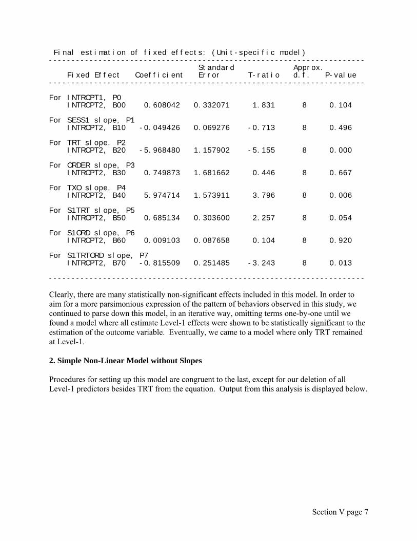
Final estimation of fixed effects: (Unit-specific model) ---------------------------------------------------------------------- Standard Approx. Fixed Effect Coefficient Error T-ratio d.f. P-value ---------------------------------------------------------------------- For INTRCPT1, P0 INTRCPT2, B00 0.608042 0.332071 1.831 8 0.104 For SESS1 slope, P1 INTRCPT2, B10 -0.049426 0.069276 -0.713 8 0.496 For TRT slope, P2 INTRCPT2, B20 -5.968480 1.157902 -5.155 8 0.000 For ORDER slope, P3 INTRCPT2, B30 0.749873 1.681662 0.446 8 0.667 For TXO slope, P4 INTRCPT2, B40 5.974714 1.573911 3.796 8 0.006 For S1TRT slope, P5 INTRCPT2, B50 0.685134 0.303600 2.257 8 0.054 For S1ORD slope, P6 INTRCPT2, B60 0.009103 0.087658 0.104 8 0.920 For S1TRTORD slope, P7 INTRCPT2, B70 -0.815509 0.251485 -3.243 8 0.013 ---------------------------------------------------------------------- Clearly, there are many statistically non-significant effects included in this model. In order to aim for a more parsimonious expression of the pattern of behaviors observed in this study, we continued to parse down this model, in an iterative way, omitting terms one-by-one until we found a model where all estimate Level-1 effects were shown to be statistically significant to the estimation of the outcome variable. Eventually, we came to a model where only TRT remained at Level-1. 2. Simple Non-Linear Model without Slopes Procedures for setting up this model are congruent to the last, except for our deletion of all Level-1 predictors besides TRT from the equation. Output from this analysis is displayed below.
Section V page 7

Summary of the model specified (in equation format) --------------------------------------------------- Level-1 Model E(Y|B) = TRIALS*P V(Y|B) = TRIALS*P(1-P) log[P/(1-P)] = P0 + P1*(TRT) Level-2 Model P0 = B00 + R0 P1 = B10 + R1 With much fewer terms in the equation, interpretation is simplified. The Level-1 equation now states that the log odds of DISRUPTR is the sum of 2 parts: the log odds at the intercept (in this case, the baseline phase overall, since trend was found to be flat), plus a term accounting for the rate of change in log odds with a phase change (treatment phase). The Level-2 equations model the intercepts and phase changes as: P0 = The average log odds during baseline for all subjects (B00), plus an error term to allow each
student to vary from this grand mean (R0). P1 = The average rate of change in log odds as a subject switches from baseline (TRT=0) to
treatment phase (TRT=1) for all students (B10), plus an error term to allow each student to vary from this grand mean (R1).
The following estimates were produced by HLM for this model: Final estimation of fixed effects: (Unit-specific model) ---------------------------------------------------------------- Standard Approx. Fixed Effect Coefficient Error T-ratio d.f. P-value ---------------------------------------------------------------- For INTRCPT1, P0 INTRCPT2, B00 0.612911 0.150045 4.085 8 0.004 For TRT slope, P1 INTRCPT2, B10 -2.363757 0.216575 -10.914 8 0.000 ---------------------------------------------------------------- When TRT=0 (i.e., the baseline phase), the overall average log odds of exhibiting a disruptive behavior for all students is 0.6129 (B00). [exp(0.6129) = 1.8568; 1.8568/2.8568= 0.6460] The expected probability of observing a disruptive behavior during the baseline phase is 0.65. The average rate of change in log odds as a student switches from baseline (TRT=0) to treatment (TRT=1) is -2.3638 (B10). This phase effect is significant as the p-value for B10 is less than .05. [exp(0.6129 – 2.3638) = exp(-1.7509) = 0.1736; 0.1736/1.1736 = 0.1479] The expected probability of observing a disruptive behavior during the treatment phase is the 0.15.
Section V page 8

Estimates of the variance components for this model (tau00 and tau11) indicate that there may be significant between-subject variation in estimates of the intercept: Final estimation of variance components: ---------------------------------------------------------------------- Random Effect Standard Variance df Chi-square P-value Deviation Component ---------------------------------------------------------------------- INTRCPT1, R0 0.34515 0.11913 8 19.53570 0.012 TRT slope, R1 0.40638 0.16514 8 13.74903 0.088 level-1, E 1.72296 2.96858 ---------------------------------------------------------------------- The between-subject variance on intercepts is estimated to be 0.1191 (tau00), which corresponds to a standard deviation of 0.3452. The p-value shown tests the null hypothesis that baseline averages for all subjects are similar. The significant p-value indicates there is a significant amount of variation between subjects on their average baseline frequencies. In other words, the variance is too big to assume it may be due only to sampling error. In order to explore the possibility that certain subject characteristics (Level-2 variables) might account for some of the between-subject variation found (i.e., that treatment might work different for different types of students), we conducted an exploratory analysis of the potential contributions of Level-2 variables. The section of output below suggests that CLASSB (the indicator that a student was in Class B, inseaad of A) might help to explain some of the between-subject variance in intercepts (see associated t-value below). Exploratory Analysis: estimated Level-2 coefficients and their standard errors obtained by regressing EB residuals on Level-2 predictors selected for possible inclusion in subsequent HLM runs ----------------------------------------------------------------
Level-1 Coefficient Potential Level-2 Predictors ----------------------------------------------------------------
CLASSB AGE WHITE PREGRADE
INTRCPT1,B0 Coefficient -0.309 -0.087 0.095 -0.113 Standard Error 0.153 0.303 0.303 0.079 t value -2.016 -0.286 0.314 -1.433
----------------------------------------------------------------
In an attempt to explain some of this between-subjects variation in baseline estimates (tau00), a final model was run entering CLASSB onto the model for the intercept (B00). 3. Simple Non-Linear Model with CLASSB on Intercept Output for this model are displayed below.
Section V page 9
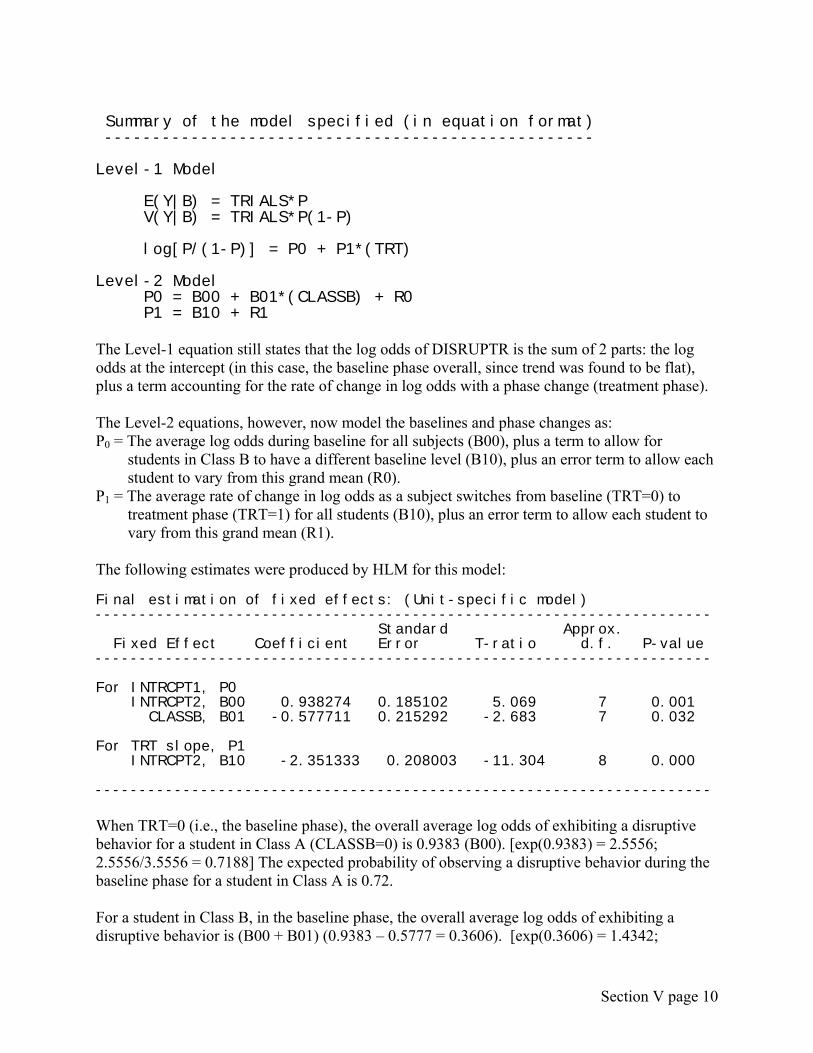
Summary of the model specified (in equation format) --------------------------------------------------- Level-1 Model E(Y|B) = TRIALS*P V(Y|B) = TRIALS*P(1-P) log[P/(1-P)] = P0 + P1*(TRT) Level-2 Model P0 = B00 + B01*(CLASSB) + R0 P1 = B10 + R1 The Level-1 equation still states that the log odds of DISRUPTR is the sum of 2 parts: the log odds at the intercept (in this case, the baseline phase overall, since trend was found to be flat), plus a term accounting for the rate of change in log odds with a phase change (treatment phase). The Level-2 equations, however, now model the baselines and phase changes as: P0 = The average log odds during baseline for all subjects (B00), plus a term to allow for
students in Class B to have a different baseline level (B10), plus an error term to allow each student to vary from this grand mean (R0).
P1 = The average rate of change in log odds as a subject switches from baseline (TRT=0) to treatment phase (TRT=1) for all students (B10), plus an error term to allow each student to vary from this grand mean (R1).
The following estimates were produced by HLM for this model: Final estimation of fixed effects: (Unit-specific model) ---------------------------------------------------------------------- Standard Approx. Fixed Effect Coefficient Error T-ratio d.f. P-value ---------------------------------------------------------------------- For INTRCPT1, P0 INTRCPT2, B00 0.938274 0.185102 5.069 7 0.001 CLASSB, B01 -0.577711 0.215292 -2.683 7 0.032 For TRT slope, P1 INTRCPT2, B10 -2.351333 0.208003 -11.304 8 0.000 ---------------------------------------------------------------------- When TRT=0 (i.e., the baseline phase), the overall average log odds of exhibiting a disruptive behavior for a student in Class A (CLASSB=0) is 0.9383 (B00). [exp(0.9383) = 2.5556; 2.5556/3.5556 = 0.7188] The expected probability of observing a disruptive behavior during the baseline phase for a student in Class A is 0.72. For a student in Class B, in the baseline phase, the overall average log odds of exhibiting a disruptive behavior is (B00 + B01) (0.9383 – 0.5777 = 0.3606). [exp(0.3606) = 1.4342;
Section V page 10

1.4342/2.4342 = 0.5892] The expected probability of observing a disruptive behavior during the baseline phase for a student in Class B is 0.59. The average rate of change in log odds as a student switches from baseline (TRT=0) to treatment (TRT=1) is -2.3638 (B10). This phase effect is significant as the p-value for B10 is less than .05. For Class A, [exp(0.9383 – 2.3513) = exp(-1.413) = 0.2434; 0.2434/1.2434= 0.1958] the expected probability of observing a disruptive behavior during the treatment phase is the 0.20. For Class B, [exp(0.9383 – 0.5777 – 2.3513) = exp(-1.9907) = 0.1366; 0.1366/1.1366 = 0.1202] the expected probability of observing a disruptive behavior during the treatment phase is the 0.12. Estimates of the variance components for this model (tau00 and tau11) indicate that there may still be significant between-subject variation in estimates of the intercept: Final estimation of variance components: ---------------------------------------------------------------------- Random Effect Standard Variance df Chi-square P-value Deviation Component ---------------------------------------------------------------------- INTRCPT1, R0 0.29867 0.08921 7 15.27190 0.032 TRT slope, R1 0.36355 0.13217 8 13.03756 0.110 level-1, E 1.73023 2.99370 ---------------------------------------------------------------------- However, it has been reduced (see variances) and the term for class in the model for the intercept did prove to significantly contribute to the estimation of the outcome variable. All in all, the estimated effect via HLM analyses is similar to that estimated via visual and descriptive analyses in the original publication. However, our HLM analyses also found a small but statistically significant different between the two classes; not in treatment effect but in starting level (baseline). Also, the original authors assumed they could average across phases (A’s: A1 and A2; B’s: B1 and B2). They were right, as we confirmed, but they did not have any basis for assuming this without checking. For these data, there are several models that fit reasonably well. No model is going to completely fit actual data because of great within-phase and within-subject variation. In a real analysis, you would compare inferences you’d make about the size of the treatment effect from the estimates derived from each model. If inferences across possible models are similar, then it doesn’t matter if you pick the “right” model or not.
Section V page 11

Alternative Methods of Coding Phases in ABAB Designs To code the four phases in an ABAB design, the most natural idea would be to have a main effect for treatment (A vs B), a main effect for the first AB phases compared with the second AB phases, and an interaction to see whether the effect of treatment is the same in both AB phase changes of the study. But many other methods of coding are possible, depending on what quantities are of interest. Here we will illustrate a nonstandard but potentially useful coding method, which we will call step coding. In some respects it resembles dummy coding, in that it only uses the numbers 0 and 1, but the coding is different in other aspects. Suppose that we want the intercept to represent behavior during the intial (baseline) phase of the study, and we want other effects to measure the changes as we go from one phase to another. That is, one effect should measure the change from A1 (the first A phase) to B1 (the first B phase); another effect should measure the next change, from B1 to A2; and the final effect should measure the final change, from A2 to B2. The coding needed to represent these effects is displayed in the following table, where the phases are labeled A1, B1, A2, and B2: Phase: A1 B1 A2 B2 A1 B1 0 1 1 1 B1 A2 0 0 1 1 A2 B2 0 0 0 1 The SPSS syntax to produce the coding for sessions and the step coding for phases is: compute sess.10 = session - 10. compute phase = 1 + trt + 2*order. compute a1b1 = (phase > 1). compute b1a2 = (phase > 2). compute a2b2 = (phase = 4). The SPSS code first creates a new variable for sessions which is the original session number minus 10; on this new variable, a 0 represents the 10th session and makes the intercept represent the child’s status on session 10 (the end of baseline). The next command creates a variable that goes from 1 to 4 to indicate the phase of the design; these are used in the following three commands to create the step coding. The meaning of these effects depends on all of them being present in the model; removing any of them changes the meanings of the remaining effects because they are not orthogonal. In the following models, we also included a term for session, coded so that 0 was the last session in the first phase of the study (phase A1). In addition, we allowed for overdispersion (as we did in fitting previous models).
Section V page 12

Discussion of model 1 Summary of the model specified (in equation format) --------------------------------------------------- The outcome variable is DISRUPT Level-1 Model E(Y|B) = TRIALS*P V(Y|B) = TRIALS*P(1-P) log[P/(1-P)] = B0 + B1*(SESS.10) + B2*(A1B1) + B3*(B1A2) + B4*(A2B2) Level-2 Model B0 = G00 + U0 B1 = G10 + U1 B2 = G20 + U2 B3 = G30 + U3 B4 = G40 + U4 This model says that (i) the logarithm of the odds of showing disruptive behavior is a function of a linear trend, as well as changes due to shifts between phases, and (ii) each of these effects may vary across individuals. Below are the estimates of the fixed effects for this model: Final estimation of fixed effects: (Unit-specific model) ---------------------------------------------------------------------- Standard Approx. Fixed Effect Coefficient Error T-ratio d.f. P-value ---------------------------------------------------------------------- For INTRCPT1, B0 INTRCPT2, G00 0.399955 0.295664 1.353 8 0.213 For SESS.10 slope, B1 INTRCPT2, G10 -0.049289 0.049237 -1.001 8 0.347 For A1B1 slope, B2 INTRCPT2, G20 -1.810020 0.642222 -2.818 8 0.023 For B1A2 slope, B3 INTRCPT2, G30 2.586380 0.438464 5.899 8 0.000 For A2B2 slope, B4 INTRCPT2, G40 -2.236028 0.451511 -4.952 8 0.001 ----------------------------------------------------------------------
Section V page 13
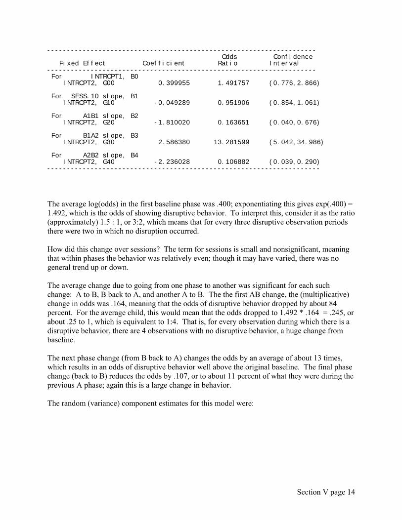
-------------------------------------------------------------------- Odds Confidence Fixed Effect Coefficient Ratio Interval -------------------------------------------------------------------- For INTRCPT1, B0 INTRCPT2, G00 0.399955 1.491757 (0.776,2.866) For SESS.10 slope, B1 INTRCPT2, G10 -0.049289 0.951906 (0.854,1.061) For A1B1 slope, B2 INTRCPT2, G20 -1.810020 0.163651 (0.040,0.676) For B1A2 slope, B3 INTRCPT2, G30 2.586380 13.281599 (5.042,34.986) For A2B2 slope, B4 INTRCPT2, G40 -2.236028 0.106882 (0.039,0.290) --------------------------------------------------------------------- The average log(odds) in the first baseline phase was .400; exponentiating this gives exp(.400) = 1.492, which is the odds of showing disruptive behavior. To interpret this, consider it as the ratio (approximately) 1.5 : 1, or 3:2, which means that for every three disruptive observation periods there were two in which no disruption occurred. How did this change over sessions? The term for sessions is small and nonsignificant, meaning that within phases the behavior was relatively even; though it may have varied, there was no general trend up or down. The average change due to going from one phase to another was significant for each such change: A to B, B back to A, and another A to B. The the first AB change, the (multiplicative) change in odds was .164, meaning that the odds of disruptive behavior dropped by about 84 percent. For the average child, this would mean that the odds dropped to 1.492 * .164 = .245, or about .25 to 1, which is equivalent to 1:4. That is, for every observation during which there is a disruptive behavior, there are 4 observations with no disruptive behavior, a huge change from baseline. The next phase change (from B back to A) changes the odds by an average of about 13 times, which results in an odds of disruptive behavior well above the original baseline. The final phase change (back to B) reduces the odds by .107, or to about 11 percent of what they were during the previous A phase; again this is a large change in behavior. The random (variance) component estimates for this model were:
Section V page 14

Sigma_squared = 2.69015 Final estimation of variance components: ----------------------------------------------------------------------------- Random Effect Standard Variance df Chi-square P-value Deviation Component ----------------------------------------------------------------------------- INTRCPT1, U0 0.70994 0.50401 8 21.85548 0.005 SESS.10 slope, U1 0.11654 0.01358 8 17.74587 0.023 A1B1 slope, U2 1.64518 2.70663 8 27.46904 0.001 B1A2 slope, U3 0.88800 0.78854 8 13.71427 0.089 A2B2 slope, U4 0.91680 0.84052 8 10.79698 0.213 level-1, R 1.64017 2.69015 ----------------------------------------------------------------------------- The random effects show that intercepts, slopes, and A1B1 effects all vary significantly across individuals, but B1A2 and A2B2 changes do not. The estimate of sigma squared is 2.69, well above the value of 1 for the model without overdispersion. We next investigate whether there is a difference between the two classrooms in which this study was conducted. We will test each effect in the design to see whether the classes differ in their general trend over session, in their status during the first phase, or during changes among the phases. Discussion of Model 2 Model 2 is specified as follows: Summary of the model specified (in equation format) --------------------------------------------------- The outcome variable is DISRUPT Level-1 Model E(Y|B) = TRIALS*P V(Y|B) = TRIALS*P(1-P) log[P/(1-P)] = B0 + B1*(SESS.10) + B2*(A1B1) + B3*(B1A2) + B4*(A2B2) Level-2 Model B0 = G00 + G01*(CLASSB) + U0 B1 = G10 + G11*(CLASSB) + U1 B2 = G20 + G21*(CLASSB) + U2 B3 = G30 + G31*(CLASSB) + U3 B4 = G40 + G41*(CLASSB) + U4 This model has the same level 1 equation as before, but each level 2 equation has a dummy variable for whether the child was (1) or was not (0) in class B. The estimates for the fixed effects in the model are in the table below:
Section V page 15

Final estimation of fixed effects: (Unit-specific model) ---------------------------------------------------------------------------- Standard Approx. Fixed Effect Coefficient Error T-ratio d.f. P-value ---------------------------------------------------------------------------- For INTRCPT1, B0 INTRCPT2, G00 -0.207357 0.365313 -0.568 7 0.588 CLASSB, G01 1.078133 0.495092 2.178 7 0.065 For SESS.10 slope, B1 INTRCPT2, G10 -0.169226 0.053472 -3.165 7 0.017 CLASSB, G11 0.209932 0.070095 2.995 7 0.021 For A1B1 slope, B2 INTRCPT2, G20 -0.335898 0.690661 -0.486 7 0.641 CLASSB, G21 -2.650404 0.946652 -2.800 7 0.027 For B1A2 slope, B3 INTRCPT2, G30 3.716603 0.517038 7.188 7 0.000 CLASSB, G31 -1.906540 0.688083 -2.771 7 0.028 For A2B2 slope, B4 INTRCPT2, G40 -1.690475 0.614778 -2.750 7 0.029 CLASSB, G41 -1.013752 0.857795 -1.182 7 0.276 ---------------------------------------------------------------------------- ---------------------------------------------------------------------- Odds Confidence Fixed Effect Coefficient Ratio Interval ---------------------------------------------------------------------- For INTRCPT1, B0 INTRCPT2, G00 -0.207357 0.812729 (0.363,1.821) CLASSB, G01 1.078133 2.939187 (0.985,8.774) For SESS.10 slope, B1 INTRCPT2, G10 -0.169226 0.844318 (0.750,0.950) CLASSB, G11 0.209932 1.233594 (1.057,1.440) For A1B1 slope, B2 INTRCPT2, G20 -0.335898 0.714696 (0.155,3.286) CLASSB, G21 -2.650404 0.070623 (0.009,0.572) For B1A2 slope, B3 INTRCPT2, G30 3.716603 41.124440 (13.124,128.862) CLASSB, G31 -1.906540 0.148594 (0.033,0.679) For A2B2 slope, B4 INTRCPT2, G40 -1.690475 0.184432 (0.047,0.717) CLASSB, G41 -1.013752 0.362855 (0.055,2.414) ----------------------------------------------------------------------
During the baseline phase, there is a large difference between the classes in disruptive behavior, although this effect barely misses statistical significance at the .05 level (again due to small sample size). In Class A, the average odds of disruptive behavior was .8, or about 4 periods of disruptive behavior for every 5 periods of nondisruptive behavior. In Class B, the average odds were (.80)(2.94) = 2.35, or nearly 5 periods of disruptive behavior for every 2 of nondisruptive behavior.
Section V page 16

The classes significantly differ in their average trend across sessions within phases. For Class A, disruptive behavior is slowly decreasing across time, regardless of phase: Each successive session has the odds decrease by .84, or about 16 percent. On the other hand, for Class B there is no time trend. The classes also differed significantly on the change from phase A1 to B1. In Class A, the odds of disruptive behavior decreased by a factor of .71, or a little over 2/3. In Class B, the odds decreased much more, by a factor of (.71)(.071) = .050 below their baseline, or to about 1/20th of their baseline rate. For the return to baseline (change from phase B1 to A2), Class A increased by an average factor of about 41 times, while Class B rebounded a smaller amount: (41.12)(.149) = 6.13. This is a large difference, and is statistically significant. The final change, from A2 to B2, was again a large drop in the average odds for class A (.18) and a somewhat larger (though not significantly different) drop for class B: (.1844)(.363) = .067. Final estimation of variance components: Sigma_squared = 2.72345 ----------------------------------------------------------------------------- Random Effect Standard Variance df Chi-square P-value Deviation Component ----------------------------------------------------------------------------- INTRCPT1, U0 0.50310 0.25311 7 12.44445 0.086 SESS.10 slope, U1 0.04522 0.00204 7 5.76728 >.500 A1B1 slope, U2 0.97555 0.95169 7 12.27001 0.091 B1A2 slope, U3 0.20672 0.04273 7 5.89174 >.500 A2B2 slope, U4 0.78245 0.61223 7 8.37865 0.300 level-1, R 1.65029 2.72345 -----------------------------------------------------------------------------
The variance components show that there is some qualitatively large variability among students within each class, but none of these is significant.
Section V page 17

Conclusion
Multilevel models provide a useful approach to modeling the behavior of individuals, where the measurements for each person comprise a short time series of the type often found in the single case design literature. These models allow us to capture variation across time in the behavior of individuals, and to determine how behavioral differences are related to person characteristics. We can easily analyze the typical types of dependent variables in single case designs: Counts during an interval (Poisson distribution) and counts of events out of a fixed number of trials (binomial distribution). However, many difficult issues arise in the analysis of even fairly simple-looking data patterns. Further work should investigate models including autoregressive parameters, although it may not be possible to get reasonable estimates of these models with so few subjects.