analyzing changing risk and planning alternatives … case... · analyzing changing risk and...

1

ANALYZING CHANGING RISK AND PLANNING ALTERNATIVES : A CASE

STUDY OF A SMALL ISLAND COUNTRY.

By:

Cees van Westen Faculty ITC, University of Twente, Netherlands

E‐mail: [email protected]

Version April 2015

2

TableofContents1. Objectives ....................................................................................................................................... 4

2. The ILWIS GIS software................................................................................................................... 6

3. Background ................................................................................................................................... 10

4. Information sources ...................................................................................................................... 12

5. Part A: Visualization of the input data ......................................................................................... 13

5.1 Input data: hazard maps ....................................................................................................... 13

5.2 Input data: Elements‐at‐risk ................................................................................................. 15

5.3 Input data: Vulnerability curves ........................................................................................... 16

5.4 Input data: administrative units........................................................................................... 17

5.5 Input data: Risk reduction alternatives ............................................................................... 18

5.5.1 Alternative 01: Engineering measures ......................................................................... 18

5.5.2 Alternative 02: Ecological measures ............................................................................ 19

5.5.3 Alternative 03: Relocation. ........................................................................................... 19

5.6 Input data: Possible future scenarios .................................................................................. 20

5.6.1 Scenario 01: Business as usual .................................................................................... 22

5.6.2 Scenario 02: Risk Informed planning ........................................................................... 23

5.6.3 Scenario 03: Worst case ............................................................................................... 25

5.6.4 Scenario 04: Realistic case ........................................................................................... 25

6. Part B: Risk analysis ...................................................................................................................... 27

6.1 Loss estimation ..................................................................................................................... 28

6.2 Risk analysis .......................................................................................................................... 30

7. Part C: Analyse the effect of possible risk reduction alternatives .............................................. 32

7.1 Loss analysis of the alternatives ........................................................................................... 32

7.2 Risk analysis of the alternatives ........................................................................................... 33

7.3 Cost benefit analysis of the alternatives .............................................................................. 34

7.3.1 Calculating the costs ..................................................................................................... 34

7.3.2 Entering the benefit values. ......................................................................................... 36

7.3.3 Net Present Value ......................................................................................................... 37

7.3.4 Internal Rate of Return ................................................................................................. 38

7.3.5 Comparing the alternatives and select the best one ................................................... 38

8. Part D: Evaluate the changes for the different scenarios. .......................................................... 39

3

8.1 Analysing the changes in land use ....................................................................................... 39

8.2 Analysing the changes in land values ................................................................................... 41

8.3 Analysing the changes in population ................................................................................... 43

8.4 Analysing the changes in risk for the different scenarios ................................................... 46

8.5 Create your own scenario ..................................................................................................... 47

8.6 Summary of your analysis .................................................................................................... 49

9. Part E: Evaluate which of the risk reduction alternatives would behave best under possible

future scenarios. ................................................................................................................................... 50

9.1 Loss calculation ..................................................................................................................... 50

9.2 Risk calculation ..................................................................................................................... 53

9.3 Cost‐benefit analysis ............................................................................................................. 56

9.4 Conclusions ........................................................................................................................... 57

10. References ................................................................................................................................. 58

4

1. Objectives

The overall aim of e use cases in this chapter is to evaluate possible changes in risk to different natural hazards, in an area along the coast of a small Caribbean island state. These changes may be related to possible risk reduction measures, but also to possible future scenarios related to land use change, population change, and climate change, and the effect of possible intervention alternatives on top of these possible future scenarios. The case study has a number of components: Part A: Analyse the input data required for such an analysis:

Hazard intensity and probability maps

Elements‐at‐risk maps in the form of land parcels and their attributes (land use type, economic value and number of people)

Vulnerability curves

Planning alternatives: in order to reduce the current risk three alternatives have been defined (engineering solutions, ecological solutions, and relocation)

Possible future scenarios: four possible future scenarios have been developed for this area: business as usual (rapid unplanned growth), risk informed planning (growth that follows the chosen alternative), worst case scenario (rapid unplanned growth combined with climate change) and climate change adaptation scenario (planned growth in a changing climatic situation)

Part B: Analyse the current risk to different hazards:

Calculate the number of elements‐at‐risk exposed to each of the hazard types and each of the return periods

Apply vulnerability matrices for estimating the vulnerability to the various hazard types.

Calculate the losses for each hazard type and return period

Integrate the losses for different return periods into annualized risk

Calculate the risk as population risk and economic risk. Part C: Analyse the effect of possible risk reduction alternatives:

Re‐calculate the risk after implementation of the risk reduction alternatives;

Determine the annual risk reduction;

Calculate the costs for implementing the risk reduction alternatives: investment costs, period of investment, maintenance costs, project lifetime;

Carry out a cost‐benefit analysis to identify the optimal alternative in terms of NPV (Net Present Value) and IRR (Internal Rate of Return)

Evaluate other factors (indicators) that are relevant in the final selection of the optimal alternative using a multi‐criteria evaluation approach.

5

Part D: Evaluate the changes for the different scenarios.

Analyse the changes in land use for the different scenarios in a number of future years (2020, 2030 and 2040) and explain the trends and possible drivers;

Analyse the changes in economic values for the different scenarios in a number of future years (2020, 2030 and 2040)

Analyse the changes in population for the different scenarios in a number of future years (2020, 2030 and 2040)

Analyse the changes in risk for the for the different scenarios in a number of future years (2020, 2030 and 2040)

Part E: Evaluate which of the risk reduction alternatives would behave best under possible future scenarios.

Analyse the changes in risk for risk reduction alternatives for the different scenarios in a number of future years (2020, 2030 and 2040);

Calculate annualized risk for each combination of risk reduction alternative and future year;

Calculate annualized risk reduction (benefit) for each combination of risk reduction alternative and future year by subtracting the annualized risk with and without the risk reduction alternative;

Use these different values for annualized risk reduction (benefits) in a cost‐benefit analysis that compares risk reduction alternatives by taking into account their behaviour under different possible future scenarios;

Determine the most “change proof” risk reduction alternative;

6

2. The ILWIS GIS software

In the development of the training materials one of the driving aspects

was that the exercises, the data and the software should be freely

available for all interested to learn about the dissemination results of the

PPRD‐EAST project. Therefore it was decided to base all the exercises on

Open Source software. We decided to use the ILWIS software, as this is

easy to learn, comprehensive and has an extensive set of tutorial material.

ILWIS is an acronym for the Integrated Land and Water Information System. It is a Geographic Information System (GIS) with Image Processing capabilities. ILWIS has been developed by the International Institute for Aerospace Survey and Earth Sciences (ITC), Enschede, The Netherlands up to release 3.3 in 2005. ILWIS comprises a complete package of image processing, spatial analysis and digital mapping. It is easy to learn and use; it has full on‐line help, extensive tutorials for direct use in courses and 25 case studies of various disciplines (See www.itc.nl)

Since July 2007, ILWIS software is freely available ('as‐is' and free of charge) as open source software (binaries and source code) under the 52°North initiative (GPL license). This software version is called ILWIS Open. ILWIS software can be downloaded for free from 52 North: http://52north.org/

As a GIS package, ILWIS allows you to input, manage, analyze and present geo‐graphical data. From the data you can generate information on the spatial and temporal patterns and processes on the earth surface.

Before you can start with the exercises you will have to download the software. We have decided to

use the version 3.4 which is not the most recent version of the ILWIS software, but one which is well

proven stable and has all the functionalities required for carrying out the exercises. The latest

versions of ILWIS have some major changes in terms of the visualisation and the exercise texts are

not adapted to that.

To install the software, please follow these steps:

Download the ILWIS software from the CHARIM website

Copy the file: Ilwis_3.4_Open.zip to your harddisk.

Unzip the file in a directory on the D (or C) drive. Not on the desktop.

Run ILWIS34Ssetup.exe to install the software.

The zip file also contains a directory Users Guide\ This folder contains the complete ILWIS 3.0 User's Guide (in .pdf format). with a file describing what changed in ILWIS 3.1. ILWIS 3.4 has new functionality, but the same file describes how to use the ILWIS 3.0 User's Guide with ILWIS 3.4. Data for these basic tutorials can be downloaded from http://www.itc.nl/ilwis/documentation/version3.asp

Before you use ILWIS first unzip the data of the first exercise (Exercise_Introduction) into a directory \exercise01\ on the C or D drive.

7

To start ILWIS, double‐click mouse the ILWIS icon on the desktop. After the opening screen you see the ILWIS Main window (see figure below). From this window you can manage your data and start all operations

Use the ILWIS Navigator (Navigation pane) to go to the sub‐ folder of the exercise. The Navigator lists all drives and directories (i.e. folders) in a tree structure.

The ILWIS Window contains a number of features:

Data catalog: displays the icons and names of the objects inside the selected directory.

Standard Toolbar: provides shortcuts for some regularly used menu commands

The Standard toolbar has the following buttons:

New Catalog Properties

Open Map Customize Catalog

Open Pixel Information List

Copy Details

Paste cd..

Delete

Navigation pane: allows for fast navigation, and can also be changed to display all operations

Menu bar: this is the main starting point for doing most of the operations in ILWIS. Check especially the options under Operations. The ILWIS Main window has six menus: File, Edit, Operations, View, Window and Help.

Command line: this is a central facility in ILWIS. Here you type calculation

8

statements (called MapCalc) which allows you to do a lot of analysis steps with raster maps. If you do an operation, the related ILWIS command is also displayed.

Object selection: this allows you to select which objects are displayed in the data catalog

Getting HELP : allows you to obtain information from any point within the program. The Help menu differs per window.

ILWIS uses different types of objects.

Data objects. Raster maps, polygon maps, segment maps, point maps, tables and columns are called data objects. They contain the actual data.

Service objects. Service objects are used by data objects; they contain accessories that data objects need besides the data itself. Domains, representations, coordinate systems and georeferences are called service objects.

9

Container objects. Container objects are collections of data objects and/or annotation: map lists, object collections, map views, layouts and annotation text.

Special objects. Special objects are histograms, sample sets, two‐dimensional tables, matrices, filters, user‐defined functions and scripts.

A vector map needs a coordinate system, a domain and a representation. These service objects are also needed for raster maps, together with another type of service object: a georeference. In this chapter we will focus our view on data and service objects.

10

3. Background

The use cases in this chapter can be used in different ways (see also the flow chart below):

A. Analyzing the current level of risk. In this workflow the stakeholders (e.g. local authorities) are interested to know the current level of risk in their municipality. They request expert organizations to provide them with hazard maps, asset maps, and vulnerability information, and use this information in risk modelling. They use the results in order to carry out a risk evaluation.

B. Analyzing the best alternatives for risk reduction. In this workflow the stakeholders want to analyse the best risk reduction alternative, or combination of alternatives. They define the alternatives, and request the expert organizations to provide them with updated hazard maps, assets information and vulnerability information reflecting the consequences of these alternatives. Once these hazard and asset maps are available for the scenarios, the new risk level is analysed, and compared with the existing risk level to estimate the level of risk reduction. This is then evaluated against the costs (both in terms of finances as well as in terms of other constraints) and the best risk reduction scenario is selected.

11

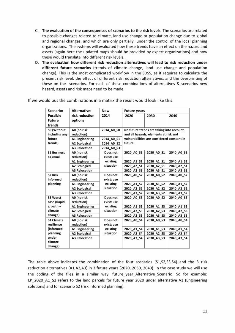
C. The evaluation of the consequences of scenarios to the risk levels. The scenarios are related to possible changes related to climate, land use change or population change due to global and regional changes, and which are only partially under the control of the local planning organizations. The systems will evaluated how these trends have an effect on the hazard and assets (again here the updated maps should be provided by expert organizations) and how these would translate into different risk levels.

D. The evaluation how different risk reduction alternatives will lead to risk reduction under different future scenarios (trends of climate change, land use change and population change). This is the most complicated workflow in the SDSS, as it requires to calculate the present risk level, the effect of different risk reduction alternatives, and the overprinting of these on the scenarios. For each of these combinations of alternatives & scenarios new hazard, assets and risk maps need to be made.

If we would put the combinations in a matrix the result would look like this:

Scenario: Possible Future trends

Alternative: risk reduction options

Now2014

Future years

2020 2030 2040

S0 (Without including any future trends)

A0 (no risk reduction)

2014_A0_S0 No future trends are taking into account, and all hazards, elements at risk and vulnerabilities are considered constant in future.

A1 Engineering 2014_A0_S1

A2 Ecological 2014_A0_S2

A3 Relocation 2014_A0_S3

S1 Business as usual


Does not exist: use existing situation

2020_A0_S1 2030_A0_S1 2040_A0_S1

A1 Engineering 2020_A1_S1 2030_A1_S1 2040_A1_S1

A2 Ecological 2020_A2_S1 2030_A2_S1 2040_A2_S1

A3 Relocation 2020_A3_S1 2030_A3_S1 2040_A3_S1

S2 Risk informed planning



2020_A0_S2 2030_A0_S2 2040_A0_S2




S3 Worst case (Rapid growth + climate change)



2020_A0_S3 2030_A0_S2 2040_A0_S3




S4 Climate resilience (informed planning under climate change)



2020_A0_S4 2030_A0_S3 2040_A0_S4




The table above indicates the combination of the four scenarios (S1,S2,S3,S4) and the 3 risk

reduction alternatives (A1,A2,A3) in 3 future years (2020, 2030, 2040). In the case study we will use

the coding of the files in a similar way: future_year_Alternative_Scenario. So for example:

LP_2020_A1_S2 refers to the land parcels for future year 2020 under alternative A1 (Engineering

solutions) and for scenario S2 (risk informed planning).

12

4. Information sources

The data set is based on original data that was prepared for an EU FP7 project SAFELAND

(http://www.safeland‐fp7.eu/) by the University of Salerno, Italy. The following persons have

developed the original hazard maps: Leonardo Cascini, Settimio Ferlisi and Sabatino Cuomo. They

also supplied the high resolution image, the DEM, building footprints, roads etc. The original hazard

maps have been modified in order to reflect the situation for the various alternatives. The land parcel

maps have all been generated by ourselves based on available high resolution images. The whole

dataset was modified to make it a generic case study reflecting a situation in an island country.

We also would like to thank Anna Scolobig from IIASA for her work on the risk reduction alternatives

(which we have taken as they were) the stakeholder involvement and the stakeholder roleplay

exercise.

Hari Narasimhan (ETH) and Emile Dopheide are thanked for their input in the cost‐benefit analysis.

Also we would like to thank Andrea Tripodi for his work in the development of the case study. Luc

Boerboom and Ziga Malek are thanked for their input in the thinking about possible future scenarios.

Kaixi Zhang is thanked for her feedback on the risk calculation method.

13

5. Part A: Visualization of the input data

The input data will be made available through a ZIP file: Case_study_Changing_Risk.zip .

Unzip the data in a directory on the harddisk (C or D drive, and not on desktop)

Open the ILWIS program and navigate to the directory where you unzipped the data

Display the raster map IMAGE and analyse what the current situation is.

(For showing in 3D in ILWIS 3.8, first select right‐click on Display Tools, select 3D properties, expand the Display Tools, expand 3D properties, double click Data Source, and select DTM.)

You can also display the hillshading image DTMShadow to get a better impression of the study area

You can also use Google Maps, Google Earth or Google Street View to navigate to the Nocera Inferiore area in Italy to check the situation yourself in more detail.

In the data window you can see the various input data which are either raster maps ( ) , polygons maps ( ), or segment maps ( ). Tables ( ) contain attribute information related to the maps. Domains ( ) are datafiles that explain what is in the maps, and can be compared to legends. Representations ( ) show how domains should displayed. Scripts ( ) are a sequenced list of ILWIS commands and expressions. By creating a script, we have combined many intermediate steps in the analysis so that you can do the exercise without knowing about GIS and ILWIS.

The study area has been affected some years ago by a landslide (in the vicinity of the quarry area, that has destroyed several buildings, and killed a number of people. The authorities in the area have become very worried because in a nearby area, a large number of debrisflows and landslides occurred some years ago. The authorities of the study area are now considering the need to carry out mitigation measures in the area as well. However, they are not sure of the type of measures and the effect of them on risk reduction, that is why they have ordered the hazard and risk study to be carried out.

5.1 Input data: hazard maps

We have made hazard maps for landslides,

debrisflows , mudflows and floods. For the work

the mudflows could be skipped if that is too much

work. The debrisflow, mudflow and flood maps have intensity data (impact pressure for mudflows

and debrisflows, and depth for flood). The landslide hazard maps do not have intensity maps, but

only spatial probability maps indicating the chance that a particular area will be affected by a

landslide.

14

The available maps are illustrated in the table below and in the figure below.

Map Hazard Return Period

Intensity Spatial probability

LS_SP_20_A0 Landslide 20 Not available yes



DF_IP_20_A0 Debrisflow 20 Impact pressure 1



FL_DE_20_A0 Flood 20 Waterdepth 1



The hazard data consists of the following components:

o Hazard type: LS= landslides, MF= mudflow, FL=Flood, DF=Debrisflows

o Return Period: this is the average frequency with which the events is expected to occur. This

is based on the analysis of the magnitude and frequency of the triggering rainfall , or of the

events themselves (e.g. flood discharge, or the number of landslides occurring in a particular

period)

o Intensity: the intensity indicates the spatially distributed effect of the hazard event. This can

be water depth for flooding, or impact pressure for debrisflows. These have been modelled

using specific hazard modelling software. These models require quite a lot of input data and

assumptions. In this exercise we will not deal with the methods how these were created. For

some types of hazards it may also not be possible to generate intensity maps, as data or

models are lacking. This is the case for landslide runout in our exercise.

15

o Spatial probability: the spatial probability indicates the chance that a particular location

would actually be affected by the hazard. This could be the result of uncertainty in the flood

modelling or runout modelling. Or it could also represent (in the absence of an intensity

map) the likelihood that a particular area will be affected by landslides based on the area of

the units, divided by the area of landslides that have occurred in the past. In this way we can

use it to reclassify so‐called landslide susceptibility maps into spatial probability maps.

o Alternatives: this indicates whether the hazard map is made for the current situation or for a

planned risk reduction alternative (A1, A2, A3)

Analyse the available hazard maps using ILWIS, by displaying them , creating histograms and by comparing the intensity and spatial probability values for the different return periods and hazard types.

You can also consult all the other maps at the same time using the Pixel Information window.

5.2 Input data: Elements‐at‐risk

We can use four types of elements‐at‐risk: building footprints, land parcels, line elements and point

elements. In the case study you will work only with land parcels. Each of them have information on:

o The use: indicating the land use type.

o The types: this is type of element‐at‐risk. Different types of

elements‐at‐risk can be affected differently by hazard events.

For the risk analysis this is important as this is linked to the

vulnerability curves, which will be explained later. The table

below gives the different types that have been used in this

exercise for buildings and for land parcels.

o The value: this is the replacement value of the elements‐at‐risk

in monetary units (Euros, US dollars etc).

o The people: the number of people that might be present in the

element‐at‐risk. Here you can decide to take the maximum

number of people or the people present at a given time (in case

when we are dealing with rapid events, the time of day/year is

also important for the population loss estimation). In this

exercise (we take here the maximum number of people.

Display the polygon map for the Land_Parcels of the current situation: LP_2014_A0_S0. Use the attriute Type to display the map. Observe the information that is available for each of the buildings. Check also the attribute table.

Display the land parcel maps for the other alternatives : LP_2014_A0. .

Compare the information of the buildings and the land parcels with repect to their attribute information on values and number of people.

16

We have made the data so that the building map and the land parcel maps have the same number of

people for the parcels in which buildings are located. For the other parcels we are using values per

m2 and multiplied these with the area of the land parcel, so that we can have an estimate of the total

maximum number of people. The same we did for the population. We took the values of the

buildings from the building footprint map, and used these for the value of the land parcels. For the

parcels without buildings we made an estimation based on the value per m2 and multiplied this with

the area.

See the Excel sheet for the detailed information, and also for calculation procedures.

We also provided some background documents that contains information on the replacement costs for the different land use types.

Displaying the hazard and elements at risk maps together. What can you conclude on the possible exposure? (We will actually calculate the exposure a bit later)

5.3 Input data: Vulnerability curves

Another very important component in the analysis are the vulnerability curves. A vulnerability curve

expresses the relation between the hazard intensity (e.g. water depth) and the degree of damage

which is expressed between 0 and 1 for a specific type of element‐at‐risk. Vulnerability curves are

derived from past disaster events by correlating observed intensities with observed damage and

deriving average regression lines from these. Vulnerability curves may also be derived through

computer modelling (e.g. finite element models where a particular uilding is exposed to a particular

intensity and the effect is calculated) or through expert opinion.

For this exercise we have made a number of vulnerability curves for all the combinations of the

hazard intensity types and the elements‐at‐risk types. We have used existing curves for the

literature, but needed to make a lot of changes as I didn’t have the curves for all of the units. The

vulnerability curves are stored in an Excel sheet. For the analysis these curves should be

implemented in the GIS (for the check analysis). I have made curves for buildings, and land parcels,

and separate curves for the physical losses (required for the economic risk analysis) and for the

population losses (people killed).

See Excel sheet: Vulnerability curves. The excel sheet contains the following vulnerability curves

Hazard type Intensity type Buildings (BU) Land parcels (LP)

Flood (FL) Waterdepth (in cm) (DE)

Physical vulnerability (PH) Population vulnerability (PO)


Debris flows and mudflows (DF)

Impact pressure (in KPa) (IP)



Landslides (LS) No intensity Single vulnerability value per type

Single vulnerability value per type

The codes in the table above indicate the various aspects of the vulnerability curves. For instance the

naming of the vulnerability curves should be as follows:

VUL_01_02_03_04:

01 refers to the hazard type (FL, DF, LS)

02 refers to the intensity measurement (WD, IP etc)

17

03 refers to the type of element at risk (BU, LP)

04 refers to the type of vulnerability (PH, PO)

For example:

VUL_FL_DE_LP_PH: Vulnerability curves for flooding, expressed in water depth, for land

parcela, and showing the physical vulnerability.

VUL_DF_IP_LP_PO: Vulnerability curves for debris flows, expressed in impact pressure, for

land parcels, and showing the population vulnerability.

Physical vulnerability curves for land parcels (for waterdepth in cm)

Physical vulnerability for debris flows (based on impact pressure in KPa )

5.4 Input data: administrative units

For the calculation of risk we also need an

administrative unit map, as we are going to

aggregate the losses eventually for particular units,

and the decision making is based on the risk within

these units. The administrative unit map contains

19 administrative units..

Display the administrative unit map on top of the image and/or the hillshading image.

0.00

0.20

0.40

0.60

0.80

1.00

1.20

0 50 100 150 200 250 300 350 400

Agricultural fields

Cultural heritage

Commercial

Farm

Natural Forest

Grassland

0.0

0.2

0.4

0.6

0.8

1.0

1.2

0 10 20 30 40

Masonry 1 floor

Masonry 2 floor

Masonry 3 floors

Reinforced concrete 1 floor

Reinforced concrete 2 floors

Reinforced Concrete 3 floors

Wooden 1 floor

18

5.5 Input data: Risk reduction alternatives

In this case study we are also evaluating three risk reduction alternatives: ‐ Alternative 1: engineering solutions ‐ Alternative 2: ecological solutions ‐ Alternative 3: relocation

5.5.1 Alternative 01: Engineering measures

This alternative aims at constructing active and passive control works using engineering measures:

Take out the soil in the landslide prone areas

Create storage basins that will retain the floods and debrisflows

Create water channels to guide the water

Create a monitoring and early warning system

We have made new land parcel maps for the alternative, and new hazard intensity maps. For the

alternative 1 we assume that the engineering works will block all debris flows and floods for return

periods up to 100 year. For return period of 200 years the engineering solutions might not be

sufficient, and the storage basins will overflow.

Display the maps related to this alternative. The map Alternative 1 shows the overall setting

The maps in the table below are the new hazard and elements‐at‐risk maps for this alternative.

Hazard type Return

period Intensity measure or spatial probability

Present situation:

Alternative 1: Engineering measures

Alternative 2: Ecological solutions

Alternative 3: Relocation

Landslide 20 Spatial Probability LS_SP_20_A0 LS_SP_20_A1 LS_SP_20_A2 LS_SP_20_A3




Debrisflow 20 Impact pressure DF_IP_020_A0 DF_IP_20_A1 DF_IP_20_A2 DF_IP_20_A3



Debrisflow 200 Impact pressure DF_IP_200_A1 DF_IP_200_A2

Flood 20 Water depth FL_DE_020_A0 FL_DE_20_A1 FL_DE_20_A2 FL_DE_20_A3



Flood 200 Water depth FL_DE_200_A1 FL_DE_200_A2

Land Parcel maps LP_2014_A0_S0 LP_2014_A1_S0 LP_2014_A2_S0 LP_2014_A3_S0

Table indicating the files names for the hazard maps and the elements‐at‐risk maps for the present

situation and for the three risk reduction alternatives.

19

5.5.2 Alternative 02: Ecological measures

This alternative aims at constructing active and passive control works using ecological solutions:

Take out the soil in the landslide prone areas

Use soil nailing in the upper slope to reduce the landslide susceptibility

Create water tanks that will retain some of the the floods

Create water channels to guide the water

A barrier of oak trees that will retain some of the debrisflows and mudflows

Create a natural park which will stop further development


The maps in the table above are the new hazard and elements‐at‐risk maps for this alternative.

5.5.3 Alternative 03:

Relocation.

This alternative aims at relocation the residential population from the most endangered administrative units indicated as blue spots in the figure :

Evacuation of the people requires that they have to be financially compensated, and that they are willing to collaborate, otherwise lengthy procedures and lawsuits are required which may take a lot of time.


The maps in the table above are the new hazard and elements‐at‐risk maps for this alternative.

20

5.6 Input data: Possible future scenarios

The analysis of changes involves the definition of a number of scenarios, which can be seen as trends, on which the users don’t have a direct influence. These can be in terms of:

Climate change: involving changes in the magnitude‐frequency of precipitation extremes and other relevant climatic stimuli (such as evaporation, days with snow cover) and in the occurrence in the time of the year of these extremes (e.g. related to changes in springtime temperature changes).

Land use change: long term land use changes relate to socio‐economic developments that might occur in an area.

Population change: also related to political and socio‐economic developments within a country.

The scenarios are possible developments, and several scenarios are possible for which it will be difficult or impossible to indicate their probability of occurrence. Scenarios of land use /land cover change can be developed using the so‐called DPSIR (European Environmental Agency, , which identify the Drivers of change (e.g. economic growth, economic crisis, changes in macro‐economic /political constellation, climate change) leading the certain pressures (e.g. increasing demand for land for residential purposes, increasing demand for natural resources), which will alter the existing state, and lead to an impact (e.g. increasing land prices, increasing risk to natural hazards, which may elicit societal response and will feedback on the drivers again (for more information, see : http://www.epa.gov/ged/tutorial/docs/DPSIR_Module_2.pdf) We would like to use four scenarios:

Name Land use change Climate change

Scenario 1 Business as usual Rapid growth without taking into account the risk information

No major change in climate expected

Scenario 2 Risk informed planning Rapid growth that takes into account the risk information and extends the alternatives in the planning

No major change in climate expected

Scenario 3 Worst case Rapid growth without taking into account the risk information

Climate change expected, leading to more frequent extreme events

Scenario 4 Most realistic Rapid growth that takes into account the risk information and extends the alternatives in the planning

Climate change expected, leading to more frequent extreme events

21

Scenario 1 (and 3) Scenario 2 (and 4)

Drivers

Pressure

State

Impact

Response

If we would put the combinations of scenarios and alternatives in a matrix the result would

look like this. The names of the elements‐at‐risk maps are given for each combination. Not

that:

for scenario 3 and 4 we are using the same element‐at‐risk maps as for scenario 1

and 2, but we change the frequency of the hazard events (the return periods);

The actual hazard maps used for the scenarios are the same as those for the

alternatives. We do not consider that the intensity will change. Only the return

periods of the hazards will change.

Possible future scenario: Now2014

Elements_at_risk maps : land_parcels

2020 2030 2040 S1 Business as usual LP_2014_A0_S0 LP_2020_A0_S1 LP_2030_A0_S1 LP_2040_A0_S1

S2 Risk informed planning LP_2014_A0_S0 LP_2020_A0_S2 LP_2030_A0_S2 LP_2040_A0_S2


LP_2014_A0_S0 LP_2020_A0_S1 LP_2030_A0_S1 LP_2040_A0_S1


LP_2014_A0_S0 LP_2020_A0_S2 LP_2030_A0_S2 LP_2040_A0_S2

The change in return periods due to climate change effects for scenario 3 and 4 are indicated

below:

New Return Period in Future Year

Old Return Period 2020 2030 2040

20 (± 5) 17 (± 6) 14 (± 7) 11 (± 8)

50 (± 10) 45 (± 12) 35 (± 14) 25 (± 16)

100 (± 20) 90 (± 23) 75 (± 26) 55 (± 30)

200 (± 40) 180 (± 44) 150 (± 49) 110 (± 53)

22

5.6.1 Scenario 01: Business as usual

This scenario is a land use change scenario only. We do not expect

a major climate change in this scenario. However the land use is

expected to change dramatically in this scenario. Land use

change will be in the form of a rapid urbanization of the study

area, occupying the flat areas from North to South. This occurs in

combination with a high demand for land leading to increasing

land prices and also to higher population densities.

The changes in land use are reflected in the land parcel map.

We use 3 future years : 2020, 2030 and 2040.

With respect to hazard types, we are considering flooding

(FL), debrisflows (DF) and landslides(LS) (and possibly

coastal hazards CO as well). We assume that the hazard

intensities and modelled areas stay the same, and the

return periods are also the same. So we can use the same

hazard maps as for the current situation.

With respect to elements‐at‐risk we are only considering

Land_Parcels. Now we take into account changes in population density and in the value of

elements‐at‐risk. We also take into account land‐use developments in the period until 2040.

For seeing the results of the modelling of values and population for the scenarios, see the Excel

sheet (Estimation of values and people for different scenarios). Also the calculation procedure is

explained there. Check this excel sheet.

We also incorporate the following four situations with respect to the design of alternatives:

o No risk reduction measures

o Engineering measures (Alternative 1)

o Ecological measures (Alternative 2)

o Relocation (Alternative 3)

If we would put the combinations in a matrix the result would look like this:

Possible future scenario:



2020 2030 2040 S1 Business as usual

A0 (no risk reduction) LP_2020_A0_S1 LP_2030_A0_S1 LP_2040_A0_S1

A1 Engineering LP_2020_A1_S1 LP_2030_A1_S1 LP_2040_A1_S1

A2 Ecological LP_2020_A2_S1 LP_2030_A2_S1 LP_2040_A2_S1

A3 Relocation LP_2020_A3_S1 LP_2030_A3_S1 LP_2040_A3_S1

23

5.6.2 Scenario 02: Risk Informed planning

In this scenario we have also rapid growth , however in the

development of the area, the risk information is taken into

consideration, and the development follows the alternatives

that have been defined. E.g. relocation will eventually lead to

relocation of all dangerous areas. Ecological alternatives will

lead to a park land area without much economic activities. In

this scenario there are no climate change effects taken into

account.


With respect to hazard types, we are considering

flooding, debrisflows and landslides. We assume that

the hazard intensities and modelled areas stay the

same, and also the return period. So we use the same

hazard maps as for the present situation

With respect to elements‐at‐risk we are only

considering Land_Parcels. We also take into account

changes in population density and in the value of

elements‐at‐risk. We also do not take into account land‐use developments in the period

until 2040. Therefore we use the land parcel maps for the present situation


24





Since this scenario uses existing maps in the database, we will indicate in the table below

which maps are used for which combination of Alternative‐Scenario‐Futur‐Year.

In the database there is no need to actually upload new maps for the specific combinations

of Alternative‐Scenario‐FutureYear. The real difference is only to assign new Return Periods

in the Hazard Data Sets. New maps are indicated in red, and new values in Orange.

We use the following maps:



Now2014


2020 2030 2040 S2 Risk informed planning

A0 (no risk reduction) Does not exist: use existing situation

LP_2020_A0_S2 LP_2030_A0_S2 LP_2040_A0_S2




25

5.6.3 Scenario 03: Worst case

This scenario is a climate change and land use change scenario. Both land use change and climate

change are expected to change dramatically in this scenario. Land use change will be in the form of a

rapid urbanization of the study area, occupying the flat areas from North to South. This occurs in

combination with a high demand for land leading to increasing land prices and also to higher

population densities. With respect to climate change, the drastic change results in an almost 50%

reduction of the return periods for the same triggering events.



With respect to hazard types, we are considering flooding, debrisflows and landslides. We

assume that the hazard intensities and modelled areas stay the same, but that the return

periods become smaller.



20 (± 5) 17 (± 6) 14 (± 7) 11 (± 8)

50 (± 10) 45 (± 12) 35 (± 14) 25 (± 16)

100 (± 20) 90 (± 23) 75 (± 26) 55 (± 30)

200 (± 40) 180 (± 44) 150 (± 49) 110 (± 53)

With respect to elements‐at‐risk we are only considering Land_Parcels. Now we take into

account changes in population density and in the value of elements‐at‐risk. We also take into

account land‐use developments in the period until 2040.









Now2014


2020 2030 2040 S3 Worst case (Rapid growth + climate change)


LP_2020_A0_S1 LP_2030_A0_S1 LP_2040_A0_S1




5.6.4 Scenario 04: Realistic case

This scenario is a climate change and land use change scenario. Both land use change and climate

change are expected to change dramatically in this scenario. In this scenario we have also rapid

growth , however in the development of the area, the risk information is taken into consideration,

and the development follows the alternatives that have been defined. E.g. relocation will eventually

lead to relocation of all dangerous areas. Ecological alternatives will lead to a park land area without

26

much economic activities. With respect to climate change, the drastic change results in an almost

50% reduction of the return periods for the same triggering events.



With respect to hazard types, we are considering flooding, debrisflows and landslides. We

assume that the hazard intensities and modelled areas stay the same, but that the return

periods become smaller.



20 (± 5) 17 (± 6) 14 (± 7) 11 (± 8)

50 (± 10) 45 (± 12) 35 (± 14) 25 (± 16)

100 (± 20) 90 (± 23) 75 (± 26) 55 (± 30)

200 (± 40) 180 (± 44) 150 (± 49) 110 (± 53)

With respect to elements‐at‐risk we are only considering Land_Parcels. Now we take into

account changes in population density and in the value of elements‐at‐risk. We also take into

account land‐use developments in the period until 2040.









Now2014


2020 2030 2040 S4 Climate resilience (informed planning under climate change)


LP_2020_A0_S2 LP_2030_A0_S2 LP_2040_A0_S2




27

6. Part B: Risk analysis

Risk is the probability of losses that may occur in the future due to different types of hazards. Hazards, such as floods, landslides, earthquakes, tsunami’s have a relation between the frequency of occurrence and the magnitude of the event. The intensity is the spatially distributed effect of a hazard event (e.g. water depth during a flood varies over an area based on the topography and other factors). Intensity maps for different return periods are obtained through hazard modelling. In this case study these data are provided for three types of hazards (floods, debrisflows, landslides). Also coastal hazards may be considered in this case study. Elements‐at‐risk are all objects, people , activities that may be affected by a hazardous event, and cause losses. The spatial overlay of hazard intensity maps and elements‐at‐risk maps is called exposure. Elements‐at‐risk exposed to a certain hazard intensity may be damaged to a certain degree. This is defined by vulnerability curves.

Loss analysis for each combination of a hazard map (for a given return period) and an elements‐at‐risk map. This done using the following steps:

Cross the intensity map with the elements‐at‐risk map. For land parcels and line elements these are subdivided into smaller units with the same intensity. For building footprints and points the maximum intensity is taken.

For each of the combination units of hazard intensity and elements‐at‐risk type, the intensity value is used in the lookup table of the vulnerability and the vulnerability value is then used. This is done separately for physical vulnerability and population vulnerability.

Then the loss is calculated: o Physical vulnerability * value * spatial probability (for economic losses) o Population vulnerability * people * spatial probability (for population losses)

Risk analysis is done after that: based on an administrative unit map, this map is crossed with the results of the loss estimation, and the losses are aggregated for the unit. When losses are calculated for at least three different hazard intensity maps with different return periods, the losses are plotted on the X‐Axis of a graph and the annual probabilities of these on the Y‐axis. The points are connected with a graph: so‐called risk curve. The area under the curve is calculated, and is define as the annual risk. The annual risk is used in the cost‐benefit analysis, where the difference in annual risk before and after the implementation of risk reduction measures (benefit) is compared with the costs of implementation.

28

6.1 Loss estimation

The Loss analysis has to be done for each combination of a hazard map (for a given return period) and an elements‐at‐risk map. Each loss estimation requires a number of steps, which make that doing this type of analysis manually is very time consuming. Therefore we are using an automated script, which combines a number of calculations and operations, and uses parameters. The script is called “Loss_calculation”. It does the following steps:

1. Rasterize the element‐at‐risk map (e.g. LP_2014_A0_S0) 2. Overlay the element at risk map with the hazard intensity map. This is done with the Cross

operation. For example the element‐at‐risk map LP_2014_A0_S0 is crossed with the hazard intensity map, e.g. FL_DE_20_A0

3. The resulting cross table (joint frequency table) contains all combinations of the land parcel code and the intensity values (e.g. water depths). Classify the results, according to the classification of the hazard intensity (e.g. domain class group FL_DE), so that the result is in the form of classes, which can be used to join with the vulnerability tables.

4. As land parcels are sometimes large and only part of them might be actually exposed to hazard intensity the script calculates the losses first for the parts of the land parcels with the same intensity.

5. In order to know which fraction of each land parcel has a certain intensity, the script reads in in the area of the whole land parcel from the attribute table of the land parcel map.

6. Then the script calculates the fraction of the land parcel (Area of the unit in the joint frequency table / the area of the entire land parcel).

7. Then the script joins with the attribute table of the land parcels and reads in the amount column either value or people, depending on the input provided by the user.)

8. The script uses this then to calculate the amount for each combination of land parcel and intensity class

9. The script joins with the attribute table of the land parcels and reads in the land use types. 10. The script joins with the vulnerability table (of the hazard type indicated) and reads in the

vulnerability values for all lands use types. The script needs to joint all 23 vulnerability types. 11. The vulnerability for each record is calculated by taking the vulnerability value of the column

that has the same land use code as in the record . 12. The script calculates a column that has an indication whether we are dealing with a spatial

probability map. This is done by creating a column SPCheck and then checking if the entered value is SP (Spatial Probability) or not.

13. If this is the case, we use the spatial probability, otherwise a value of 1. 14. The script then calculates the loss by multiplying the amount * vulnerability * spatial

probability. 15. In order to bring back the information at the level of the land parcels, the script aggregates

the loss for the land parcels and put the results in the table Results_LP 16. The script also aggregates the loss for the administrative units and stores the results in the

Table Results_Admin_units 17. The script aggregates the losses for the whole area and stores the results in the Table

Result_Total_area 18. The script then deletes all the intermediate files

Open the script Loss_calculation and have a look at the codes. We don’t ask you now to understand it.

29

The script stores the results in three tables:

Results_LP : the results for each land parcel. Generally this is too detailed.

Results_Admin_Unit: the results are stored per administrative unit. This is the level for which we want to calculate the risk.

Results_Total_Area: the results aggregated for the entire area. If you do a cost‐benefit analysis, using single values for the entire area could be used.

It is not really required that you understand each individual step of the analysis, because we have combined them into one file, called a script file that contains all above calculation steps. You can run the total analysis in one go. the only thing you need to specify is: for which combinations of hazard type, return period, and element‐at‐risk map do I make the loss assessment. This is done by indicating the variables in a script. the Loss_calculation script has the following variables. The script uses nine parameters, which you can change everytime, so you can use the script for all possible combinations:

%1 = Hazard Type (e.g. FL, DF, LS)

%2 = Intensity measure (e.g. DE, IP)

%3 = Return period (e.g. 020)

%4 = Future Year (2014, 2020, 2030, 2040)

%5 = Risk reduction alternative (A0, A1, A2,A3)

%6 = Scenario (S1, S2, S3, S4)

%7 = Physical or population Risk (PH or PO)

%8 = Value or People (If you select PH for %5 you should select Value, otherwise People)

%9 = Spatial Probability (either 1 or the letters SP)

You can run the script in various ways. On the command line type:

Run Loss_calculation

Open the script and press the run button. Then the following input screen shows . Fill in the right values. Make sure for the return period to fill in values without decimals (so 20 and not 20.000) and also for the future year.

Automate the loss calculation for many combinations You can also run the script bypassing the input screen. You can do that by typing the parameters behind the script name, separeted by spaces. For instance, on the command line:

Run Loss_calculation FL DE 20 2014 A0 S0 PH value You can also prepare an input script where you write all the combinations for which you want to calculate losses.

Open the script Loss_Input where you can adjust all the input lines, and after that run the input script. The script contains all the combinations of hazard maps , return periods, and alternatives for the current situation.

Make sure the input script contains the following lines: Run Loss_calculation FL DE 20 2014 A0 S0 PH value Run Loss_calculation FL DE 50 2014 A0 S0 PH value Run Loss_calculation FL DE 100 2014 A0 S0 PH value

30

Run Loss_calculation DF IP 20 2014 A0 S0 PH value Run Loss_calculation DF IP 50 2014 A0 S0 PH value Run Loss_calculation DF IP 100 2014 A0 S0 PH value Run Loss_calculation LS SP 20 2014 A0 S0 PH value Run Loss_calculation LS SP 50 2014 A0 S0 PH value Run Loss_calculation LS SP 100 2014 A0 S0 PH value

When you type : Run Loss_input and all the loss calculations are done in one go (it will take some minutes).

Check the results in the tables: Results_LP, Results_admin_units and Results_total_area.

6.2 Risk analysis

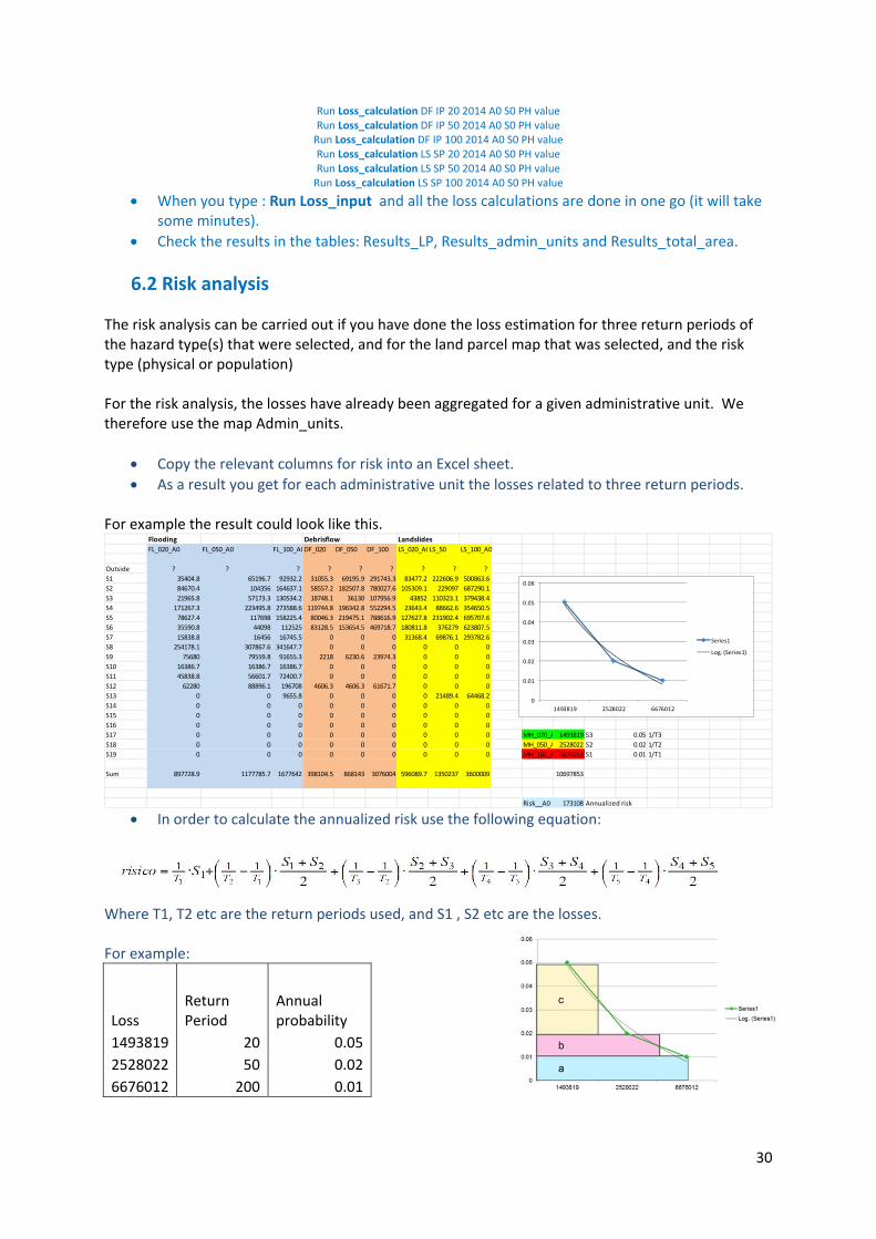
The risk analysis can be carried out if you have done the loss estimation for three return periods of the hazard type(s) that were selected, and for the land parcel map that was selected, and the risk type (physical or population) For the risk analysis, the losses have already been aggregated for a given administrative unit. We therefore use the map Admin_units.

Copy the relevant columns for risk into an Excel sheet.

As a result you get for each administrative unit the losses related to three return periods. For example the result could look like this.

In order to calculate the annualized risk use the following equation:

Where T1, T2 etc are the return periods used, and S1 , S2 etc are the losses. For example:

Loss Return Period

Annual probability

1493819 20 0.05

2528022 50 0.02

6676012 200 0.01

Flooding Debrisflow Landslides

FL_020_A0 FL_050_A0 FL_100_A0DF_020 DF_050 DF_100 LS_020_A0LS_50 LS_100_A0

Outside ? ? ? ? ? ? ? ? ?

S1 35404.8 65196.7 92932.2 31055.3 69195.9 291743.3 83477.2 222606.9 500863.6

S2 84670.4 104356 164637.1 58557.2 182507.8 780027.6 105309.1 229097 687290.1

S3 21965.8 57173.3 130534.2 18748.1 36130 107956.9 43852 110323.1 379438.4

S4 171267.3 223495.8 273588.6 119744.8 196342.8 552294.5 23643.4 88662.6 354650.5

S5 78627.4 117698 158225.4 80046.3 219475.1 788616.9 127627.8 231902.4 695707.6

S6 35590.8 44098 112525 83128.5 153654.5 469718.7 180811.8 376279 623807.5

S7 15838.8 16456 16745.5 0 0 0 31368.4 69876.1 293782.6

S8 254178.1 307867.6 341647.7 0 0 0 0 0 0

S9 75680 79559.8 91655.3 2218 6230.6 23974.3 0 0 0

S10 16386.7 16386.7 16386.7 0 0 0 0 0 0

S11 45838.8 56601.7 72400.7 0 0 0 0 0 0

S12 62280 88896.1 196708 4606.3 4606.3 61671.7 0 0 0

S13 0 0 9655.8 0 0 0 0 21489.4 64468.2

S14 0 0 0 0 0 0 0 0 0

S15 0 0 0 0 0 0 0 0 0

S16 0 0 0 0 0 0 0 0 0

S17 0 0 0 0 0 0 0 0 0 MH_020_A 1493819 S3 0.05 1/T3

S18 0 0 0 0 0 0 0 0 0 MH_050_A 2528022 S2 0.02 1/T2

S19 0 0 0 0 0 0 0 0 0 MH_100_A 6676012 S1 0.01 1/T1

Sum 897728.9 1177785.7 1677642 398104.5 868143 3076004 596089.7 1350237 3600009 10697853

Risk__A0 173108 Annualized risk

0

0.01

0.02

0.03

0.04

0.05

0.06

1493819 2528022 6676012

Series1

Log. (Series1)

31

Annual risk: = 0.01*6676012+(0.02‐0.01)*( 6676012+2528022)/2+(0.05‐0.02)*( 2528022+1493819)/2= 173108

When you are doing this for different hazard types it is also important to decide if the hazard types are dependent or not. This means if they are related to the same triggering event. In our case the hazards are all related to the same triggering: rainfall. This is important for the estimation of the risk, where we take the maximum loss per administrative unit of the various hazards, and do not add them up. We would therefore not add the losses for different hazards, but would take the maximum losses for each of the hazards. The risk analysis can also be done using a script: Risk_calculation. It can only be executed after you have calculated the losses using the script Loss_calculation. The data should be available in the table: Results_LP. It requires the individual losses for Floods (FL), Debrisflow (DF) and Landslides (LS) for three return periods. This script does the following:

For each land parcel it will calculate the maximum loss for the same return period resulting either from flooding, landslides or debrisflows, as these events are caused by the same trigger.

Then the resulting losses are aggregated by the administrative units;

Then the annual risk is calculated using the equation indicated above; The script uses the following parameters: %1 = Year %2 = Alternative %3 = Scenario %4 = First return period %5 = Second return period %6 = Third return period The three return periods %4 , %5 and %6 allow us later to change the return periods in scenarios 3 and 4 where we assume that due to climate change the frequency of the hazard events will increase. We will run the risk analysis for the current situation: Year = 2014 Alternative = A0 Scenario = S0 First return period = 20 Second return period = 50 Third return period = 100

Run the script Risk_Calculation and fill in these parameters. Make sure to delete the decimals for year, and return periods.

When the calculation is finished, open the table Risk_Results, and find out:

The administrative units with the highest risk

The total annualized risk for the entire area.

32

7. Part C: Analyse the effect of possible risk

reduction alternatives

After knowing how you calculate the loss using the script Loss_calculation and how to generate the risk curve using the script Risk_calculation, as was explained in the previous exercise, we will now evaluate the possibilities for risk reduction. The results of the previous exercise show the resulting loss values for the three hazard types (flooding, debrisflows and landslides) for different return periods (1 in 20 years, 1 in 50 years and 1 in 100 years). The results show the losses for the 19 administrative units in the study area. As you can see (see resulting table from the previous exercise) the results show that in some of the administrative units the risk is higher than in others. For instance administrative units 4,5 and 6 have high potential losses for all three hazards. Unit 8 has only flood losses. Unit 13 has predominantly landslide losses. You can also see that the average annual losses for the entire area, based on the three hazards are high: 173 thousand Dollars per year. Therefore it is important to take action and plan for risk reduction measures to reduce the risk A similar calculation can be done for population losses. The results for that also show that in some of the administrative units the population losses are high. This is the basis for evaluating which risk reduction alternatives would be the best to implement. In this exercise we will identify three risk reduction alternatives and reanalyse the risk, the calculate the risk reduction (which is the average annual risk after the implementation minus the current average annual risk). We will later also make an estimation of the costs for the alternatives and carry out a cost‐benefit analysis.



Now2014

Average Annual risk

Risk reduction



2014_A0_S0




7.1 Loss analysis of the alternatives

The first step to do is to reanalyse the losses , but now for the new situations that would exist if the risk reduction alternatives would be implemented. In the animation above you have seen the various input maps that are required for each of the three alternatives. They are also summarized in the three table below, whihc gives the example for alternative 1. As you can see from the animation, depending on the proposed risk reduction alternative, both hazard maps and elements‐and‐risk maps should be updated. For alternative 1: both hazard maps and elements‐at‐risk maps should be updated. Constructing the engineering measures will greatly reduce the flood, debrisflow and landslide hazards. However, as the most eastern watershed is not considered in the plans, there the flood and debris flow hazard will remain the same. The engineering works have been designed for a return period of 100 years. Therefore we have also modelled the 1 in 200 year event, and for this situation the engineering works will be partly overtopped. The construction of the storage basins requires to change the land

33

use and relocate some of the houses which are in the location of the storage basins. Therefore also a new elements‐at‐risk map is needed. For alternative 2: also both hazard maps and elements‐at‐risk maps should be remade, as they both will change as a consequence of the risk reduction alternative. The plantation of the protective forest will greatly reduce the hazards, however, not as much as the construction of the engineering works. It will also take a number of years before the trees in the protective forest are tall enough to have their full protection function. Also for the plantation of the protective forest some land parcels will have to cgange their land use and some buildings have to be relocated. For alternative 3 (relocation) only the elements will change. This alternative doesn't involve the reduction of hazards, but only the reduction of the exposed elements‐at‐risk (buildings). therefore the same hazard maps can be used as for the current situation. Similarly as the analysis which was done for the current risk we are doing this analysis in two steps:

‐ Loss analysis for each individual combination of hazard set (for a given date, hazard type and return period) and elements‐at‐risk (the land parcel map for the given scenario and future year).

‐ Risk analysis by combining the loss results for different hazards and return periods.

Loss analysis. We will use the script Loss_calculation for that.

Adapt the script Loss_input and add the specific combinations of alternatives, hazard types and elements‐at‐risk

The best is to copy the text in a text editor and adjust the parameters like the alternative.

The example on the right side show the situation for alternative 1

After generating the input script, you can run it and one by one the actual loss estimation script (Loss_calculation) is calculated, everytime with another set of input data.

Each time the results of the analysis are written in three tables with the results: Results_LP (for each landparcel the results are stored), Result_Admin_Units (results aggregated per administrative units) and Results_Total (Aggregated values for the entire area).

The calculation might take some time (probably about 15 minutes)

When the calculation is completed, check the results from the tables indicated above.

7.2 Risk analysis of the alternatives

The risk analysis which was done using a scrip Risk_calculation (see previous exercises) can now also be done for the different scenarios. Remember that the script has the following vairables:

%1 = Year %2 = Alternative %3 = Scenario %4 = First return period %5 = Second return period %6 = Third return period

We assume that flooding, landslides and debrisflows are depending on the same trigger, so we take the maximum losses for a given area from one of the three hazards. We assume that if a triggering events occurs it may trigger either landslides, flashfloods or debrisflows, and the area affected by

34

one would lead to a certain amount of losses. If another event also happens it will not cause twice the same damage. The input data for the risk analysis is handled through the scrip Risk_calculation_input. For running the alternatives 1 to 3 the following information should be available: Note that we first calculate the current risk, and then calculate the risk for the three alternatives.

Adapt the Risk_calculation_input script so that it represents the same situation as the one shown above.

Then run the script by typing on the command line: Run Risk_calculation_input

Next you use the script Risk_calculation with the input script Risk_calculation_ input, which should contain the following lines:

run risk_calculation 2014 A0 S0 20 50 100 run risk_calculation 2014 A1 S0 20 50 100 run risk_calculation 2014 A2 S0 20 50 100 run risk_calculation 2014 A3 S0 20 50 100

Run the script.

Copy to the results to an Excel table, and present them in a graph in which you show the average annual risk before and after the implementation of the alternative, and calculate the difference, which is the annual risk reduction or benefit;

7.3 Cost benefit analysis of the alternatives

After calculating the risk curves and annual risk for the current situation and for one or more of the

three alternatives, you can analyse which of the alternatives leads to the highest risk reduction (the

largest benefit). However, the costs for the alternative might be much higher. Therefore it is

important to also analyse the cost‐benefit relation.

7.3.1 Calculating the costs

In order to do that you need to estimate the costs for each of the alternatives. For that you need to

analyse:

The initial investment costs

The period over which these investment costs are made

In which year after the start of the construction are the benefits achieved.

The annual maintenance costs

The total duration of the project. In our case we will use a project lifetime of 50 years.

The initial investment costs are composed of all the costs needed to carry out the alternative. The

implementation of each alternative will have a number of components that each costs money. The

first part of the analysis is to identify all the individual cost options. The table below shows an

example of these.

Item Alternative 1: Engineering solutions

Alternative 2:Ecological solutions

Alternative 3: Relocation.

Item related to construction costs

Expropriating existing houses where green belt is constructed

Expropriating existing houses where green belt is constructed

Expropriating existing houses

35

Expropriating land where green belt is constructed

Expropriating land where green belt is constructed

Lawsuits

Construction of retention basins Planting trees Construction of new buildings (or)

Slope stabilization Constructing water tanks Giving compensation to expropriated owners

Slope stabilization

How long does the construction take?

In which year does the benefit start?

Annual maintenance costs

Project lifetime 50 years

The following aspects should be considered:

Items related to construction cost Time of construction

Benefit starts Annual Maintenance

Alternative 1: engineering solutions

Storage basins Slope stabilization Expropriation of land and

existing buildings where construction will take place

3 years 4th year From year 4


Expropriation of land and existing buildings where construction will take place

Slope stabilization Water tank construction

3 years From 4th year with 100% benefit in 10th year

From year 2


Compensation of owners of buildings

Expropriation of existing buildings

Lawsuits

10 years 100% benefit starts from 11th year

From year 11

36

For each of these items you need to make an estimation. The costs

estimation can be done in the following ways:

Calculating the area of land that will change. You can do that using the building maps or the land parcel maps of the present situation and of the alternatives (e.g. LP_2014_A0 as land parcel map of the current situation). This map also has value information and information on the number of people. When you overlay these with the land parcel map for the alternative (e.g. LP_2014_A1 for the parcel map of the first alternative) you can calculate how much area of land will change and their values.

You can also calculate the area of the land that is converted from the current situation to for example the tree belt under Alternative 2, or the number of retention basin under Alternative 1. You can then use values per m2 in the calculation.

Make an estimation of the unit costs per m2 that you are using in the analysis, or ask the staff for these values. See also the suggested values on the right side

Prepare an Excel sheet in which you make a line for each year, and a column for each of the components of the cost analysis. See example below:

Year Alternative 1: Engineering solutions

Alternative 2: Ecological solutions Alternative 3: Relocation

Storage basin construction

Slope stabilization

Maintenance

Total Expropriation

Tree planting

Slope stabilization

Maintenance

Total Expropriating existing houses

New buildings

Financial compen sation

Maintenance

Total

2014

2015

2016

2017

2018

2019

2020

2021

2022

2023

etc

2030

Etc

2040

etc

After filling in the values in the Excel sheet you can also calculate the overall costs per year for each of the alternatives (the columns: Total)

7.3.2 Entering the benefit values.

37

In the previous part of the exercise the benefits in terms of risk reduction have been calculated. The

table below gives a summary of the calculated reduction in annual risk reduction. The calculation on

the following pages gives the results of these calculation:

Current situation Alternative 1 Alternative 2 Alternative 3

Annualized risk

Risk Reduction ‐

Calculate the Risk Reduction (as the annualized risk for the current situation minus the annualized risk for the alternative) for the 3 alternatives.

Decide in which year the Risk Reduction will actually start. It may be possible that in the first years you have investments, but no risk reduction yet, as the alternative to reduce the risk is not finished.

Think about this for the 3 alternatives and decide in which year we will actually reach the risk reduction.

In the Excel sheet add for each of the alternatives a column, called Risk Reduction for each of the scenarios.

In the Excel sheet calculate the Incremental Benefits, by Calculating the difference between the Risk Reduction and the total of the costs per year. For the first years these values might be negative.

7.3.3 Net Present Value

We need to take into account that the same amount of money in the future will be less valuable

today. We will need therefore to calculate the so‐called net present value (NPV).

The Net Present Value (NPV) calculates the net present value of an investment by using a discount

rate and a series of future payments (negative values) and income (positive values).

Rate: is the rate of discount over the length of one period

Value 1 value 2 … are the “arguments” representing the payments and income.

NPV = the discounted benefits and costs at a given discount rate.

An example is given below:

38

In the Excel worksheet to the right of the table make a cell NPV ( Net Present Value) ;

In the cell next to it insert the name Interest rate (which is the same as discount rate) and enter the value of : 10 %.

In Excel: Click in your “NPV” cell and Insert Function; select Financial Functions.

Select: NPV

The Function Arguments Box opens ( see figure below);

Select for Interest Rate 6%

For value 1: select the whole column down all the incremental benefits; starting at year 1 up to year 40.

Click OK

Repeat the NPV calculation, but now with different discount rates

7.3.4 Internal Rate of Return

Now we are going to calculate the Internal rate of return. The Internal Rate of Return is the discount

rate/interest rate at which the NPV=0

In Excel: Click Insert Function and select Financial Functions.

Select: IRR

The Function Arguments Box opens;

Read the HELP file

For values: select the whole column down all the incremental benefits; starting at year 1 up to year 40.

Click OK.

7.3.5 Comparing the alternatives and select the best one

Now we will compare the NPV and IRR values for the various risk reduction alternatives.

Calculate the NPV and IRR for the three alternatives. Calculate the NPV for 3 interest rates

Compare the results.

Decide which of the three alternatives is the best based on the cost‐benefit evaluation.

NPV at 5 % interest rate



IRR

Alternative 1

Alternative 2

Alternative 3

39

8. Part D: Evaluate the changes for the different

scenarios.

The aim of this component is to analyse the changes in land use, values and population over time due to the different scenarios and the alternatives, and to describe the drivers, pressures , and changes. We do this using the land parcel maps for the different combinations. We have generated the various land parcel maps in such a way that they have the same polygon boundaries, but the contents (attributes: type, value and population) change from one situation to another.

Check that the polygon boundaries are the same by comparing different land parcel maps.

Use the PixelInfo programme and load in the series of land parcels maps that you would like to compare. Moving over the map with the mouse will show you how land use types change

from period to another.

8.1 Analysing the changes in land use

For analysing the changes in landuse we are going to calculate the area per land use type for the various land parcel maps of the scenarios, future years and alternatives.

Create a new table Results_landuse_change, using the domain landuse

In this table join with the table LP_2014_A0_S0 and aggregate the Area , grouping by Type.

Check the results in the table Results_landuse_change You can also automate this procedure using the script Landuse_change. This script uses three parameters: %1 = The scenario (S0,S1,S2) %2 = The alternative (A0,A1,A2,A3) %3 = The year

Open the script and check the statement.

Run the script for a particular combination of alternative, scenario and year. Best is to do that for the combination marked red in the table on the next page.

Adjust the script Landuse_change_input by entering the combinations that you want to analyse.

The example to the right shows how the Landuse_change_input script could be for analysing the changes in senario1

You can run this script by typing on the command line:

Run landuse_change_input

Present the results in a table, and in a graph in which you show the change in area per land use through time for the different scenarios and alternative combinations.

Discuss the results of the land use change given the particular scenario and alternative, and indicate:

Which developments in land use type do you observe?

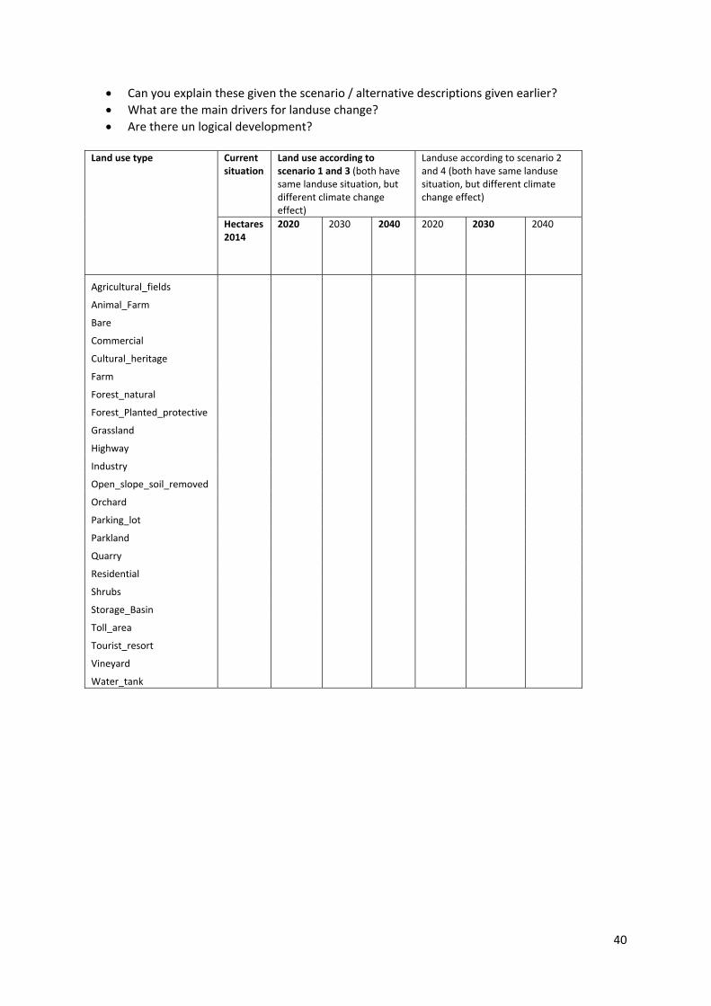
40

Can you explain these given the scenario / alternative descriptions given earlier?

What are the main drivers for landuse change?

Are there un logical development? Land use type Current

situation Land use according to scenario 1 and 3 (both have same landuse situation, but different climate change effect)

Landuse according to scenario 2 and 4 (both have same landuse situation, but different climate change effect)

Hectares 2014

2020 2030 2040 2020 2030 2040

Agricultural_fields

Animal_Farm

Bare

Commercial

Cultural_heritage

Farm

Forest_natural

Forest_Planted_protective

Grassland

Highway

Industry

Open_slope_soil_removed

Orchard

Parking_lot

Parkland

Quarry

Residential

Shrubs

Storage_Basin

Toll_area

Tourist_resort

Vineyard

Water_tank

41

8.2 Analysing the changes in land values

Land values are indicated per land parcel for each of the future scenarios and future years. The land values were estimated based on the land use. The values include the objects on the land and the values represent the replacement costs. In the value estimation the effect of inflation is not considered so that it is better to compare the situation of the different years. The following table gives the changes in land value per land use type: Estimated values for scenarios 1 and 3. Land use type Value

per m2 2014

Value per hectare 2014

Increase per year

Value per m2 2020

Increase per year

Value per m2 2030

increase per year

Value per m2 2040

Agricultural_fields 0.2 2000 0.01 0.2 0.01 0.2 0.01 0.3

Animal_Farm 300.0 3000000 0 300.0 0 300.0 0 300.0

Bare 0.0 0 0 0.0 0 0.0 0 0.0

Commercial 237.0 2370000 0.01 251.6 0.01 277.9 0.01 307.0

Cultural_heritage 396.0 3960000 0.02 446.0 0.02 543.6 0.02 662.7

Farm 211.0 2110000 0 211.0 0 211.0 0 211.0

Forest_natural 11.0 110000 0 11.0 0 11.0 0 11.0

Forest_Planted_protective 13.0 130000 0 13.0 0 13.0 0 13.0

Grassland 0.1 1000 0 0.1 0 0.1 0 0.1

Highway 250.0 2500000 0 250.0 0 250.0 0 250.0

Industry 300.0 3000000 0 300.0 0 300.0 0 300.0

Open_slope_soil_removed 0.0 0 0 0.0 0 0.0 0 0.0

Orchard 2.5 25000 0.01 2.7 0.01 2.9 0.03 3.9

Parking_lot 150.0 1500000 0 150.0 0.01 165.7 0.03 222.7

Parkland 15.0 150000 0 15.0 0 15.0 0 15.0

Quarry 0.1 1000 0 0.1 0 0.1 0 0.1

Residential 300.0 3000000 0.01 318.5 0.02 388.2 0.03 521.7

Shrubs 0.0 100 0 0.0 0 0.0 0 0.0

Storage_Basin 50.0 500000 0 50.0 0 50.0 0 50.0

Toll_area 350.0 3500000 0 350.0 0 350.0 0 350.0

Tourist_resort 266.0 2660000 0.02 299.6 0.03 402.6 0.04 595.9

Vineyard 12.0 120000 0.03 14.3 0.04 21.2 0.06 38.0

Water_tank 30.0 300000 0 30.0 0 30.0 0 30.0

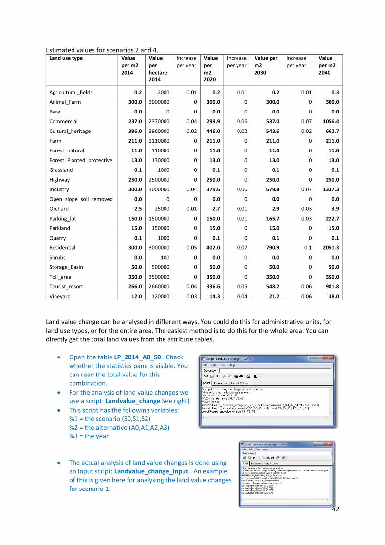
42

Estimated values for scenarios 2 and 4. Land use type Value

per m2 2014

Value per hectare 2014

Increase per year

Value per m2 2020

Increase per year

Value per m2 2030

increase per year

Value per m2 2040

Agricultural_fields 0.2 2000 0.01 0.2 0.01 0.2 0.01 0.3

Animal_Farm 300.0 3000000 0 300.0 0 300.0 0 300.0

Bare 0.0 0 0 0.0 0 0.0 0 0.0

Commercial 237.0 2370000 0.04 299.9 0.06 537.0 0.07 1056.4

Cultural_heritage 396.0 3960000 0.02 446.0 0.02 543.6 0.02 662.7

Farm 211.0 2110000 0 211.0 0 211.0 0 211.0

Forest_natural 11.0 110000 0 11.0 0 11.0 0 11.0

Forest_Planted_protective 13.0 130000 0 13.0 0 13.0 0 13.0

Grassland 0.1 1000 0 0.1 0 0.1 0 0.1

Highway 250.0 2500000 0 250.0 0 250.0 0 250.0

Industry 300.0 3000000 0.04 379.6 0.06 679.8 0.07 1337.3

Open_slope_soil_removed 0.0 0 0 0.0 0 0.0 0 0.0

Orchard 2.5 25000 0.01 2.7 0.01 2.9 0.03 3.9

Parking_lot 150.0 1500000 0 150.0 0.01 165.7 0.03 222.7

Parkland 15.0 150000 0 15.0 0 15.0 0 15.0

Quarry 0.1 1000 0 0.1 0 0.1 0 0.1

Residential 300.0 3000000 0.05 402.0 0.07 790.9 0.1 2051.3

Shrubs 0.0 100 0 0.0 0 0.0 0 0.0

Storage_Basin 50.0 500000 0 50.0 0 50.0 0 50.0

Toll_area 350.0 3500000 0 350.0 0 350.0 0 350.0

Tourist_resort 266.0 2660000 0.04 336.6 0.05 548.2 0.06 981.8

Vineyard 12.0 120000 0.03 14.3 0.04 21.2 0.06 38.0

Land value change can be analysed in different ways. You could do this for administrative units, for land use types, or for the entire area. The easiest method is to do this for the whole area. You can directly get the total land values from the attribute tables.

Open the table LP_2014_A0_S0. Check whether the statistics pane is visible. You can read the total value for this combination.

For the analysis of land value changes we use a script: Landvalue_change See right)

This script has the following variables: %1 = the scenario (S0,S1,S2) %2 = the alternative (A0,A1,A2,A3) %3 = the year

The actual analysis of land value changes is done using an input script: Landvalue_change_input. An example of this is given here for analysing the land value changes for scenario 1.

43

Run this script by typing: Run Landvalue_change_input

Adjust the Landvalue_change_input script so that also the other scenarios are included. Do this by copying the content in a text editor and changing them.

Then run the input script and after the calculation is done, investigate the results and write them in a table like the one below.

Note that the results for scenario 1 and 3 and for scenario 2 and 4 are the same as the land use for scenario 3 is the same as for scenario 1 and the ones from scenario 4 the same as scenario 2 (only the frequency of hazard events changes due to climate change effects).


Current situation

Future years






8.3 Analysing the changes in population

Also population densities and number of people are indicated per land parcel for each of the future scenarios and future years. The population data were estimated based on the land use. The number of people are considered maximum values, and not specific population scenarios (e.g. daytime night‐time, summer / winter etc.) have been considered. The tables below show the data on the basis of which the estimations were made: Scenario 1 and 3: Population data Land use type People

per m2 2014

People per hectare2014

Increase per year

People per m2 2020

Increase per year

People per m2 2030

increase per year

People per m2 2040


Agricultural_fields 0.00001 1 0 0.00001 0 0.00001 0 0.00001 1

Animal_Farm 0.00005 5 0 0.00005 0 0.00005 0 0.00005 5

Bare 0.00000 0 0 0.00000 0 0.00000 0 0.00000 0

Commercial 0.00500 500 0 0.00500 0 0.00500 0 0.00500 500

Cultural_heritage 0.00100 100 0 0.00100 0 0.00100 0 0.00100 100

Farm 0.00005 5 0 0.00005 0 0.00005 0 0.00005 5

Forest_natural 0.00001 1 0 0.00001 0 0.00001 0 0.00001 1

Forest_Planted_protective 0.00002 2 0 0.00002 0 0.00002 0 0.00002 2

Grassland 0.00000 0.1 0 0.00000 0 0.00000 0 0.00000 0

Highway 0.00500 500 0 0.00500 0 0.00500 0 0.00500 500

Industry 0.00100 100 0 0.00100 0 0.00100 0 0.00100 100

Open_slope_soil_removed 0.00000 0 0 0.00000 0 0.00000 0 0.00000 0

44

Orchard 0.00003 2.5 0 0.00003 0 0.00003 0 0.00003 3

Parking_lot 0.00100 100 0 0.00100 0 0.00100 0 0.00100 100

Parkland 0.00020 20 0 0.00020 0 0.00020 0 0.00020 20

Quarry 0.00005 5 0 0.00005 0 0.00005 0 0.00005 5

Residential 0.00040 40 0.01 0.00042 0.02 0.00052 0.03 0.00070 70

Shrubs 0.00000 0 0 0.00000 0 0.00000 0 0.00000 0

Storage_Basin 0.00000 0 0 0.00000 0 0.00000 0 0.00000 0

Toll_area 0.00500 500 0 0.00500 0 0.00500 0 0.00500 500

Tourist_resort 0.00150 150 0 0.00150 0 0.00150 0 0.00150 150

Vineyard 0.00020 20 0 0.00020 0 0.00020 0 0.00020 20

Water_tank 0.00000 0 0 0.00000 0 0.00000 0 0.00000 0

Scenario 2 and 4: Population data Land use type People

per m2 2014


Increase per year

People per m2 2020

Increase per year

People per m2 2030

increase per year

People per m2 2040


Agricultural_fields 0.00001 1 0 0.00001 0 0.00001 0 0.00001 1

Animal_Farm 0.00005 5 0 0.00005 0 0.00005 0 0.00005 5

Bare 0.00000 0 0 0.00000 0 0.00000 0 0.00000 0

Commercial 0.00500 500 0 0.00500 0 0.00500 0 0.00500 500

Cultural_heritage 0.00100 100 0 0.00100 0 0.00100 0 0.00100 100

Farm 0.00005 5 0 0.00005 0 0.00005 0 0.00005 5

Forest_natural 0.00001 1 0 0.00001 0 0.00001 0 0.00001 1

Forest_Planted_protective 0.00002 2 0 0.00002 0 0.00002 0 0.00002 2

Grassland 0.00000 0.1 0 0.00000 0 0.00000 0 0.00000 0

Highway 0.00500 500 0 0.00500 0 0.00500 0 0.00500 500

Industry 0.00100 100 0 0.00100 0 0.00100 0 0.00100 100

Open_slope_soil_removed 0.00000 0 0 0.00000 0 0.00000 0 0.00000 0

Orchard 0.00003 2.5 0 0.00003 0 0.00003 0 0.00003 3

Parking_lot 0.00100 100 0 0.00100 0 0.00100 0 0.00100 100

Parkland 0.00020 20 0 0.00020 0 0.00020 0 0.00020 20

Quarry 0.00005 5 0 0.00005 0 0.00005 0 0.00005 5

Residential 0.00040 40 0.05 0.00054 0.1 0.00139 0.1 0.00361 361

Shrubs 0.00000 0 0 0.00000 0 0.00000 0 0.00000 0

Storage_Basin 0.00000 0 0 0.00000 0 0.00000 0 0.00000 0

45

Toll_area 0.00500 500 0 0.00500 0 0.00500 0 0.00500 500

Tourist_resort 0.00150 150 0 0.00150 0 0.00150 0 0.00150 150

Vineyard 0.00020 20 0 0.00020 0 0.00020 0 0.00020 20

Water_tank 0.00000 0 0 0.00000 0 0.00000 0 0.00000 0

Population change can be analysed in different ways. You could do this for administrative units, for land use types, or for the entire area. The easiest method is to do this for the whole area. You can directly get the total population values from the attribute tables.

Open the table LP_2014_A0_S0. Check whether the statistics pane is visible. You can read the population information for this combination.

For the analysis of land value changes we use a script: Population_change See right)

This script has the following variables: %1 = the scenario (S0,S1,S2) %2 = the alternative (A0,A1,A2,A3) %3 = the year

The actual analysis of population changes is done using an input script: Population_change_input. An example of this is given here for analysing the population changes for scenario 1.

Run this script by typing:

Run Population_change_input

Adjust the Population_change_input script so that also the other scenarios are included. Do this by copying the content in a text editor and changing them.

Then run the input script and after the calculation is done, investigate the results and write them in a table like the one below.

Note that the results for scenario 1 and 3 and for scenario 2 and 4 are the same as the land use for scenario 3 is the same as for scenario 1 and the ones from scenario 4 the same as scenario 2 (only the frequency of hazard events changes due to climate change effects).


Current situation

Future years





46

8.4 Analysing the changes in risk for the different scenarios

Similarly as the analysis which was done for the current risk and for the evaluation of the best risk reduction alternative, we are doing this analysis in two steps:

‐ Loss analysis for each individual combination of hazard set (for a given date, hazard type and return period) and elements‐at‐risk (the land parcel map for the given scenario and future year).

‐ Risk analysis by combining the loss results for different hazards and return periods. Loss analysis. You can also analyse the changes in risk for the different scenarios. This will take more time, but you can use the script Loss_calculation for that.

Adapt the script Loss_input and add the specific combinations of scenarios, and future years

The best is to copy the text in a text editor and adjust the parameters like the future year and the scenario number.

The example on the right side show the situation for the scenario 1 for the current situation and for 3 future years: 2020, 2030 and 2040.

After generating the input script, you can run it and one by one the actual loss estimation script (Loss_calculation) is calculated, everytime with another set of input data.

Each time the results of the analysis are written in three tables with the results: Results_LP (for each landparcel the results are stored), Result_Admin_Units (results aggregated per administrative units) and Results_Total (Aggregated values for the entire area).

The calculation might take quite some time (probably at least one hour, since many calculations have to be made)

When the calculation is completed, check the results from the tables indicated above. Risk analysis The risk analysis which was done using a scrip Risk_calculation (see previous exercises) can now also be done for the different scenarios. Remember that the script has the following vairables:

%1 = Year %2 = Alternative %3 = Scenario %4 = First return period %5 = Second return period %6 = Third return period

We assume that flooding, landslides and debrisflows are depending on the same trigger, so we take the maximum losses for a given area from one of the three hazards. We assume that if a triggering events occurs it may trigger either landslides, flashfloods or debrisflows, and the area affected by one would lead to a certain amount of losses. If another event also happens it will not cause twice the same damage.

47

The input data for the risk analysis is handled through the scrip Risk_calculation_input. For running the scenarios 1 to 4 the following information should be available: Note that we first calculate the current risk, and then calculate the risk for the four different scenarios.

Scenario 1 and 2 use the same return periods as the current situation, as both of these scenarios only consider land use changes, and the losses for these were calculated in the loss calculation. There is no climate change effect considered, so therefore we use the same return periods as for the current situation.

However for scenarios 2 and 4 we adjust the return periods based on the change in expected frequencies that are coming from the climate change analysis. The table with these values was presented in the beginning in the section dealing with the input data.

Adapt the Risk_calculation_input script so that it represents the same situation as the one shown above.

Then run the script by typing on the command line: Run Risk_calculation_input

Calculate the annualized risk for the combinations indicated and put these in the table




Future years

2020 2030 2040

S1 Business as usual A0 (no risk reduction)

S2 Risk informed planning A0 (no risk reduction)





8.5 Create your own scenario

Optionally it would also be nice if you could also make your own scenario, and change the land use

types for the different future years based on your own assumptions. We are not going to use any

land use change model, but use logical reasoning instead. The idea is that future land use

developments should also take into account:

Avoid hazardous areas as much as possible;

Possible coastal hazards (storm surges and tsunamis) which would prohibit constructions

close to the coast;

48

Incorporate for population increase of 10% per decade;

You can do this using the following approach:

In the table LP_2014_A0_S0 create a new column Type_2020_A0_S5 which has the same landuse as 2014 by using the following equation in the table:

Type_2020_A0_S5:=Type

Overlay with the largest return periods of the hazard maps (DF_IP_100_A0, FL_DE_100_A0 and LS_IP_100_A0) using transparancies. Use pixelinfo and load in these maps.

Double click on a polygon of the map LP_2014_A0_S0 and change the land use type for 2020, and continue to do so for all relevant polygons.

Create a column Type_2030_A0_S5:= Type_2020_A0_S5 and edit the new changes.

Create a column Type_2040_A0_S5:= Type_2030_A0_S5 and edit the new changes.

Calculate the population changes, using the data from the Excel sheet (Estimation of values and people for different scenarios).

Analyse the changes in land use for the new scenario in the future years (2020, 2030 and 2040) and explain the trends and possible drivers;

49

8.6 Summary of your analysis

After analysing the land use change, land value change and population change, you can now give a more thorough evaluation of the changes and the drivers.

Analyse the changes in land use for the different scenarios in a number of future years (2020,

2030 and 2040) and explain the trends and possible drivers;

Analyse the changes in economic values for the different scenarios in a number of future years (2020, 2030 and 2040)

Analyse the changes in population for the different scenarios in a number of future years (2020, 2030 and 2040)

Analyse the changes in risk for the for the different scenarios in a number of future years (2020, 2030 and 2040)

50

9. Part E: Evaluate which of the risk reduction

alternatives would behave best under possible

future scenarios.

This part integrates the previous components. It will allow you to analyse which risk reduction alternative is the best change‐proof. The analysis follows the following steps:

Analyse the changes in risk for risk reduction alternatives for the different scenarios in a number of future years (2020, 2030 and 2040);

Calculate annualized risk for each combination of risk reduction alternative and future year;

Calculate annualized risk reduction (benefit) for each combination of risk reduction alternative and future year by subtracting the annualized risk with and without the risk reduction alternative;

Use these different values for annualized risk reduction (benefits) in a cost‐benefit analysis that compares risk reduction alternatives by taking inot account their behaviour under different possible future scenarios;

Determine the most “change proof” risk reduction alternative;

9.1 Loss calculation

The table below shows all combinations for scenario S1 , the no risk reduction situation, and the

three risk reduction alternatives, for 4 future years. For each combination there are 3 loss maps for

flooding (for 20, 50 and 100 year return period), 4 for debrisflows and 3 for landslides.



Now 2014

Future years

2020 2030 2040


A0 (no risk reduction) 2014_A0_S0 No future trends are taking into account, and all hazards, elements at risk and vulnerabilities are considered constant in future.




S1 Business as usual A0 (no risk reduction) Does not exist: use existing situation

2020_A0_S1 2030_A0_S1 2040_A0_S1






2020_A0_S2 2030_A0_S2 2040_A0_S2






2020_A0_S3 2030_A0_S2 2040_A0_S3




S4 Climate resilience (informed planning under


2020_A0_S4 2030_A0_S3 2040_A0_S4


51

climate change) A2 Ecological 2020_A2_S4 2030_A2_S3 2040_A2_S4


The cells in the table above all have a specific combination of elements‐at‐risk and hazard maps. For instance for the first two scenarios the following maps are needed. Red (e.g. LP_2020_A0_S1) = elements‐at‐risk maps. Green (e.g. FL_DE_020_A1) = hazard maps

SCenario Alternative 2020 2030 2040

S1 Business as usual A0 (no risk reduction) LP_2020_A0_S1 LP_2030_A0_S1 LP_2040_A0_S1

Landslides: LS_SP_020_A0, LS_SP_050_A0, LS_SP_100_A0 Floods: FL_DE_020_A0, FL_DE_050_A0, FL_DE_100_A0 Debrisflow: DF_IP_020_A0, DF_IP_050_A0, DF_IP_100_A0








A0 (no risk reduction) LP_2020_A0_S2 LP_2020_A0_S2 LP_2020_A0_S2








For these combinations the loss assessment needs to be done. The script Loss_Calculation has the following variables: %1 = Hazard Type (e.g. FL, DF, LS) %2 = Intensity measure (e.g. DE, IP) %3 = Return period (e.g. 020) %4 = Future Year (2014, 2020, 2030, 2040) %5 = Risk reduction alternative (A0, A1, A2,A3) %6 = Scenario (S1, S2, S3, S4) %7 = Physical or population Risk (PH or PO) %8 = Value or People (If you select PH for %5 you should select Value, otherwise People)

52

Adapt the script Loss_input and add the specific combinations of scenarios, alternatives and future years that you want to analyse.

The table on the next page shows all the loss combinations that should be calculated for scenario 1 in order to be able to calculate the multi‐hazard risk. So for each combination of scenario, future year and alternative we have loss for three hazard types (floods, landslides and debrisflow) and each of these for three return periods (20 , 50 and 100 years). For scenario 2 this would look similarly.

For scenario 3 the losses are basically the same as for scenario 1, because we are using the same land use scenario, and the same hazard maps. Only the frequency of the hazard events will differ, but this has not effect on the individual losses, but only on the risk .

The Loss_input script might need many lines, with different combinations of scenario, year, alternative, hazard type and return period. You can use a text editor to copy and past, and find&replace text easier.

Once the Loss_input script is completed, run it. It will take a considerable amount of time, so a coffee break might be useful

After completion it might be good to copy the result file: Result_LP to another directory as a back‐up.

The results will look like the ones in the table below:

Step Alternative: risk reduction options

Future years

2020 2030 2040

S1 Business as usual A0 (no risk reduction) Flood losses:

FL_20_2020_A0_S1_PH FL_50_2020_A0_S1_PH FL_100_2020_A0_S1_PH Debris flow losses DF_20_2020_A0_S1_PH DF_50_2020_A0_S1_PH DF_100_2020_A0_S1_PH Landslide losses LS_20_2020_A0_S1_PH LS_50_2020_A0_S1_PH

LS_100_2020_A0_S1_PH

Flood losses

FL_20_2030_A0_S1_PH FL_50_2030_A0_S1_PH FL_100_2030_A0_S1_PH Debris flow losses DF_20_2030_A0_S1_PH DF_50_2030_A0_S1_PH DF_100_2030_A0_S1_PH Landslide losses LS_20_2030_A0_S1_PH LS_50_2030_A0_S1_PH

LS_100_2030_A0_S1_PH

Flood losses FL_20_2040_A0_S1_PH FL_50_2040_A0_S1_PH FL_100_2040_A0_S1_PH Debris flow losses DF_20_2040_A0_S1_PH DF_50_2040_A0_S1_PH DF_100_2040_A0_S1_PH Landslide losses LS_20_2040_A0_S1_PH LS_50_2040_A0_S1_PH LS_100_2040_A0_S1_PH

A1 Engineering FL_20_2020_A1_S1_PH

FL_50_2020_A1_S1_PH FL_100_2020_A1_S1_PH DF_20_2020_A1_S1_PH DF_50_2020_A1_S1_PH DF_100_2020_A1_S1_PH LS_20_2020_A1_S1_PH LS_50_2020_A1_S1_PH

LS_100_2020_A1_S1_PH

FL_20_2030_A1_S1_PH


LS_100_2030_A1_S1_PH

FL_20_2040_A1_S1_PH FL_50_2040_A1_S1_PH FL_100_2040_A1_S1_PH DF_20_2040_A1_S1_PH DF_50_2040_A1_S1_PH DF_100_2040_A1_S1_PH LS_20_2040_A1_S1_PH LS_50_2040_A1_S1_PH LS_100_2040_A1_S1_PH

A2 Ecological FL_20_2020_A2_S1_PH


LS_100_2020_A2_S1_PH

FL_20_2030_A2_S1_PH


LS_100_2030_A2_S1_PH


53

A3 Relocation FL_20_2020_A3_S1_PH


LS_100_2020_A3_S1_PH

FL_20_2030_A3_S1_PH

FL_50_2030_A3_S1_PH FL_100_2030_A3_S1_PH DFL_20_2030_A3_S1_PH DF_50_2030_A3_S1_PH DF_100_2030_A3_S1_PH LS_20_2030_A3_S1_PH LS_50_2030_A3_S1_PH

LS_100_2030_A3_S1_PH



A0 (no risk reduction) Not filled in here because of the limited space but they would be looking like the ones filled in for

scenario 1. A1 Engineering

A2 Ecological

A3 Relocation

S3 Worst case (Rapid growth +

climate change)

A0 (no risk reduction) Losses same as S1 A0 Losses same as S1 A0 Losses same as S1 A0

A1 Engineering Losses same as S1 A1 Losses same as S1 A1 Losses same as S1 A1

A2 Ecological Losses same as S1 A2 Losses same as S1 A2 Losses same as S1 A2

A3 Relocation Losses same as S1 A3 Losses same as S1 A3 Losses same as S1 A3

S4 Climate resilience (informed planning under climate

change)

A0 (no risk reduction) Losses same as S2 A0 Losses same as S2 A0 Losses same as S2 A0

A1 Engineering Losses same as S2 A1 Losses same as S2 A1 Losses same as S2 A1

A2 Ecological Losses same as S2 A2 Losses same as S2 A2 Losses same as S2 A2

A3 Relocation Losses same as S2 A3 Losses same as S2 A3 Losses same as S2 A3

9.2 Risk calculation

Also the risk assessment script (Risk_calculation) has to be run for many combinations, basically for each combination of scenario, future year and alternative. Remember that the script Risk_calculation requires the following variables:

%1 = Year %2 = Alternativer %3 = Scenario %4 = First return period %5 = Second return period %6 = Third return period

Adapt the script Risk_input and add the specific combinations of scenarios, alternatives and future years that you want to analyse. `The example to the right shows the possible combinations for scenarios 1 and 2

Run the script Risk_Input and calculate the Annualized risk for the specific combinations of scenarios, alternatives and future years of scenario 1 and 2. These are the results indicated below in the green part in the table below.

Copy the results into an Excel table , so that for each combination you have an Average Annual Risk value.

54



Future years

2020 2030 2040 S1 Business as usual A0 (no risk reduction) Losses

AR_2020_A0_S1) Annualized risk (AR_2030_A0_S1)

Annualized risk(AR_2040_A0_S1)

A1 Engineering AR_2020_A1_S1 AR_2030_A1_S1 AR_2040_A1_S1

A2 Ecological AR_2020_A2_S1 AR_2030_A2_S1 AR_2040_A2_S1

A3 Relocation AR_2020_A3_S1 AR_2030_A3_S1 AR_2040_A3_S1


A0 (no risk reduction) AR_2020_A0_S2 AR_2030_A0_S2 AR_2040_A0_S2

A1 Engineering AR_2020_A1_S2 AR_2030_A1_S2 AR_2040_A1_S2

A2 Ecological AR_2020_A2_S2 AR_2030_A2_S2 AR_2040_A2_S2

A3 Relocation AR_2020_A3_S2 AR_2030_A3_S2 AR_2040_A3_S2



A1 Engineering

A2 Ecological

A3 Relocation



A1 Engineering

A2 Ecological

A3 Relocation

Calculate the Risk Reduction for the specific combinations of scenarios, alternatives and

future years of scenario 1 and 2. These are the results indicated below in the green part

below:



Future years

2020 2030 2040 S1 Business as usual A0 (no risk reduction) Losses

AR_2020_A0_S1) Annualized risk (AR_2030_A0_S1)

Annualized risk(AR_2040_A0_S1)

A1 Engineering Risk reduction =AR_2020_A0_S1 ‐ AR_2020_A1_S1

Risk reduction = AR_2030_A0_S1 ‐ AR_2030_A1_S1

Risk reduction =AR_2040_A0_S1 ‐ AR_2040_A1_S1

A2 Ecological Risk reduction =AR_2020_A0_S1 ‐ AR_2020_A2_S1



A3 Relocation Risk reduction =AR_2020_A0_S1 ‐ AR_2020_A3_S1




A0 (no risk reduction) Risk reduction =AR_2020_A0_S2 ‐ AR_2020_A0_S2



A1 Engineering Risk reduction =AR_2020_A0_S2 ‐ AR_2020_A1_S2


Risk reduction =AR_2040_A0_S2 AR_2040_A1_S2

A2 Ecological Risk reduction =AR_2020_A0_S2 ‐ AR_2020_A2_S2



A3 Relocation Risk reduction =AR_2020_A0_S2 ‐ AR_2020_A3_S2





A1 Engineering

A2 Ecological

A3 Relocation



A1 Engineering

A2 Ecological

A3 Relocation

For calculating the Annualized risk for the specific combinations of scenarios, alternatives and future years of scenario 3 and 4, we can use the calculated losses of scenario 1 and 2 and change the

55

frequency (return periods and annual probability ) of the hazards as indicated in the table below while taken the same values for the losses as for scenario 1 and scenario 2. These are the results indicated below in the green part

New Return Period in Future Year for scenarios 3 and 4


20 17 14 11

50 45 35 25

100 90 75 55

200 180 150 110

In the script Risk_input you can do that by adding the new return periods, for example:

Scenario 1: Scenario 3

run risk_calculation 2020 A0 S1 20 50 100 run risk_calculation 2030 A0 S1 20 50 100 run risk_calculation 2040 A0 S1 20 50 100 etc

run risk_calculation 2020 A0 S1 17 45 90 run risk_calculation 2030 A0 S1 14 35 75 run risk_calculation 2040 A0 S1 11 25 55 etc

Adapt the script Risk_input and add the specific combinations of scenarios, alternatives and future years that you want to analyse.

Run the script Risk_Input and calculate the Annualized risk for the specific combinations of scenarios, alternatives and future years of scenario 3 and 4. These are the results indicated below in the yellow part.

Calculate the annualized risk for the combinations indicated and put these in an Excel table.

Calculate the benefits for each situation by subtracting the annualized risk after implementation of a risk reduction alternative from the one before that.



Future years

2020 2030 2040 S1 Business as usual A0 (no risk reduction)

A1 Engineering Benefit S1 A1 2020

Benefit S1 A1 2030

Benefit S1 A1 2040

A2 Ecological Benefit S1 A2 2020

Benefit S1 A2 2030

Benefit S1 A2 2040

A3 Relocation Benefit S1 A32020

Benefit S1 A3 2030

Benefit S1 A3 2040

S2 Risk informed planning A0 (no risk reduction)


Benefit S2 A1 2030

Benefit S2 A2 2040


Benefit S2 A2 2030

Benefit S2 A2 2040


Benefit S2 A3 2030

Benefit S2 A3 2040




Benefit S3 A1 2030

Benefit S3 A1 2040


Benefit S3 A2 2030

Benefit S3 A2 2040


Benefit S3 A3 2030

Benefit S3 A3 2040




Benefit S4 A1 2030

Benefit S4 A2 2040


Benefit S4 A2 2030

Benefit S4 A2 2040

A3 Relocation Benefit S4 Benefit S4 A3 Benefit S4 A3 2040

56

A32020 2030

9.3 Cost‐benefit analysis

Once the benefits have been calculated, the cost‐benefit can be calculated. If you compare the

method explained in section 6.1 , the cost calculation stays the same, but the values for risk

reduction (the benefits) are now different for future years (the ones indicated in red below). These

values come from the benefits (annualized risk before – annualized risk after implementation of a

risk reduction alternative). The orange values inbetween are interpolated values between the

calculated ones (in the red cells).

Scenario 1 Year Alternative 1: Engineering

solutions Alternative 2: Ecological solutions Alternative 3: Relocation

Costs Risk Reduction

Incremental benefit

NPV

IRR


Incremental benefit

NPV

IRR


Incremental benefit

NPV IRR

2014

2015

2016

2017

2018

2019

2020 Benefit S1 A1 2020

Benefit S1 A2 2020

Benefit S1 A3 2020

2021

2022

2023

etc

2030 Benefit S1 A1 2030

Benefit S1 A2 2030

Benefit S1 A3 2030

Etc

2040 Benefit S1 A1 2040

Benefit S1 A2 2040

Benefit S1 A3 2040

etc

2064

Create in Excel 4 tables with the cost‐benefit calculations for the scenarios.

Calculate the Net Present Value and Internal Rate of Return for the Scenarios

57

9.4 Conclusions

Finally , in your report and presentation for this case study, present the results of part B, C, D,E.

We hope you are able to provide an answer to the questions:

Which risk reduction alternative is the best now?

Which risk reduction alternative is the best for each of the 4 scenarios?

Which is the most “change proof” risk reduction alternative?

In which scenario does the risk increase most?

In which scenario do we have the best development?

What would be the added effect of coastal hazards on the results?


Alternative: risk reduction options NPV IRR Which one is

best? S1 Business as usual

A1 Engineering

A2 Ecological

A3 Relocation


A1 Engineering

A2 Ecological

A3 Relocation


A1 Engineering

A2 Ecological

A3 Relocation


A1 Engineering

A2 Ecological

A3 Relocation

58

10. References

Cascini, L., Ferlisi, S., Sorbino,G. and Cuomo, S. (2011). Report of the activities carried out by the research group of Unisa. Deliverable D2.11. QRA case studies at selected “hotspots”. SafeLand. Living with landslide risk in Europe: Assessment, effects of global change, and risk management strategies. http://www.safeland‐fp7.eu/results/Documents/D2.11.pdf

Scolobig, A., J. Bayer, L. Cascini, Settimio Ferlisi (2011) Design and testing: a risk communication strategy and a deliberative process for choosing a set of mitigation and prevention measures. Deliverable D5.7. SafeLand. Living with landslide risk in Europe: Assessment, effects of global change, and risk management strategies http://www.safeland‐fp7.eu/results/Documents/D5.7.pdf

Narasimhan , H. , Faber , M. (2011) Quantitative risk‐cost‐benefit analysis of selected mitigation options for two case studies. Deliverable D5.3.. SafeLand. Living with landslide risk in Europe: Assessment, effects of global change, and risk management strategies http://www.safeland‐fp7.eu/results/Documents/D5.3_revised.pdf

59

Results.

42: Calculating risk for the current situation

The results show the resulting loss values for the three hazard types (flooding, debrisflows and

landslides) for different return periods (1 in 20 years, 1 in 50 years and 1 in 100 years). The table

shows the results for the 19 administrative units. As you can see the results show that in some of the

administrative units the risk is higher than in others. For instance administrative units 4,5 and 6 have

high potential losses for all three hazards. Unit 8 has only flood losses. Unit 13 has predominatly

landslide losses. You can also see that the average annual losses for the entire area, based on the

three hazards are high: 173 thousand Dollars per year. Therefore it is important to take action and

plan for risk reduction measures to reduce the risk.

A similar calculation can be done for population losses.

4.3

Calculation of average annual risk after the implementation of the alternatives:

Flooding Debrisflow Landslides

FL_020_A0 FL_050_A0 FL_100_A0DF_020 DF_050 DF_100 LS_020_A0LS_50 LS_100_A0

Outside ? ? ? ? ? ? ? ? ?

S1 35404.8 65196.7 92932.2 31055.3 69195.9 291743.3 83477.2 222606.9 500863.6

S2 84670.4 104356 164637.1 58557.2 182507.8 780027.6 105309.1 229097 687290.1

S3 21965.8 57173.3 130534.2 18748.1 36130 107956.9 43852 110323.1 379438.4

S4 171267.3 223495.8 273588.6 119744.8 196342.8 552294.5 23643.4 88662.6 354650.5

S5 78627.4 117698 158225.4 80046.3 219475.1 788616.9 127627.8 231902.4 695707.6

S6 35590.8 44098 112525 83128.5 153654.5 469718.7 180811.8 376279 623807.5

S7 15838.8 16456 16745.5 0 0 0 31368.4 69876.1 293782.6

S8 254178.1 307867.6 341647.7 0 0 0 0 0 0

S9 75680 79559.8 91655.3 2218 6230.6 23974.3 0 0 0

S10 16386.7 16386.7 16386.7 0 0 0 0 0 0

S11 45838.8 56601.7 72400.7 0 0 0 0 0 0

S12 62280 88896.1 196708 4606.3 4606.3 61671.7 0 0 0

S13 0 0 9655.8 0 0 0 0 21489.4 64468.2

S14 0 0 0 0 0 0 0 0 0

S15 0 0 0 0 0 0 0 0 0

S16 0 0 0 0 0 0 0 0 0

S17 0 0 0 0 0 0 0 0 0 MH_020_A 1493819 S3 0.05 1/T3

S18 0 0 0 0 0 0 0 0 0 MH_050_A 2528022 S2 0.02 1/T2

S19 0 0 0 0 0 0 0 0 0 MH_100_A 6676012 S1 0.01 1/T1

Sum 897728.9 1177785.7 1677642 398104.5 868143 3076004 596089.7 1350237 3600009 10697853

Risk__A0 173108 Annualized risk

0

0.01

0.02

0.03

0.04

0.05

0.06

1493819 2528022 6676012

Series1

Log. (Series1)

60

Cost estimation:

Items related to construction cost Time of construction

Benefit starts Annual Maintenance

Alternative 1: engineering solutions

Storage basins Slope stabilization Expropriation of land and

existing buildings where construction will take place

3 years 4th year From year 4


Expropriation of land and existing buildings where construction will take place

Slope stabilization Water tank construction

3 years From 4th year with 100% benefit in 10th year

From year 2


Compensation of owners of buildings

Expropriation of existing buildings

Lawsuits

10 years 100% benefit starts from 11th year

From year 11

61

Costs for alternative 1:

Results CBA Alternative 1:

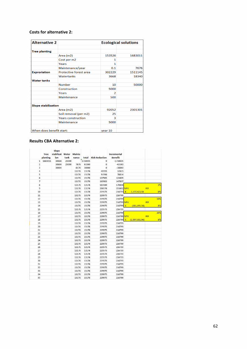
62



63



Summary results Cost‐Benefit analysis:

NPV at 5% Interest Rate



IRR

Alternative 1: Engineering solutions

€ 2,430,104.23 € 415,033.92 ‐ € 556,029.09 12%


€ 1,197,423.50 ‐ € 381,695.56 ‐ € 1,097,601.96 8%

Alternative 3: Relocation ‐ € 10,207,900.66 ‐ € 8,531,766.17 ‐ € 5,992,954.80 ‐5%

This means that alternative 3 is always the worst one": the NPV values are always negative.

Alternative 1 (Engineering solutions) is the best one, although the differences with alternative 2

(Ecological solutions) are not so very high.

64

Which alternative would be selected is not only depending on the Cost‐Benefit analysis . Also many

other factors might play a role, and the stakeholders might have other reasons why they would

prefer one particular alternative. Therefore a Multi‐Criteria evaluation would be the best next step,

in which stakeholders can bring in other indicators (social, environmental, legislation, support by

population etc.) and wight them against the risk related indicators and cost‐benefit related

indicators.

65

44: Analyzing the changes related to different scenarios.

Results Land use change

Land use according to scenario 1 and 3 (both have same landuse situation, but different climate change effect)


2014 2020 2030 2040 2020 2030 2040

Agricultural_fields 85205 54342 0 0 24435 4301 4301

Animal_Farm 9639 9639 4301 0 9639 9639 9639

Bare 31354 2785 2042 0 1314 743 743

Commercial 18772 61989 90410 151300 25144 36918 42070

Cultural_heritage 4289 4289 4831 4831 4289 4289 4289

Farm 117829 99823 67847 42893 110705 98036 91086

Forest_natural 2687779 2674466 2667449 2685162 2678630 2671613 2690797

Forest_Planted_protective 309301 304793 332458 332458 362170 362170 362170

Grassland 35890 39970 16558 16558 39645 20461 16558

Highway 55811 55811 55811 55811 55811 55811 55811

Industry 44465 55188 63389 76736 44465 39750 39750

Orchard 665137 618232 517087 357962 632086 582562 560447

Parking_lot 1166 5063 13858 17281 1166 1622 1622

Parkland 18556 33679 70149 74450 39868 58919 54722

Quarry 115095 128408 140650 140650 128408 140650 140650

Residential 125954 194402 327795 465811 195936 279402 335971

Shrubs 90855 69325 63607 43445 35471 31374 9569

Toll_area 13960 13960 13960 13960 13960 13960 13960

Tourist_resort 22934 47884 64110 76705 30619 49581 49581

Vineyard 293786 273729 231465 191764 314016 285976 264041

Water_tank 2813 2813 2813 2813 2813 2813 2813

Percentage change with respect to the current situation



2020 2030 2040 2020 2030 2040

Agricultural_fields 63.8 0.0 0.0 28.7 5.0 5.0

Animal_Farm 100.0 44.6 0.0 100.0 100.0 100.0

Bare 8.9 6.5 0.0 4.2 2.4 2.4

Commercial 330.2 481.6 806.0 133.9 196.7 224.1

Cultural_heritage 100.0 112.6 112.6 100.0 100.0 100.0

Farm 84.7 57.6 36.4 94.0 83.2 77.3

66

Forest_natural 99.5 99.2 99.9 99.7 99.4 100.1

Forest_Planted_protective 98.5 107.5 107.5 117.1 117.1 117.1

Grassland 111.4 46.1 46.1 110.5 57.0 46.1

Highway 100.0 100.0 100.0 100.0 100.0 100.0

Industry 124.1 142.6 172.6 100.0 89.4 89.4

Orchard 92.9 77.7 53.8 95.0 87.6 84.3

Parking_lot 434.2 1188.5 1482.1 100.0 139.1 139.1

Parkland 181.5 378.0 401.2 214.9 317.5 294.9

Quarry 111.6 122.2 122.2 111.6 122.2 122.2

Residential 154.3 260.2 369.8 155.6 221.8 266.7

Shrubs 76.3 70.0 47.8 39.0 34.5 10.5

Toll_area 100.0 100.0 100.0 100.0 100.0 100.0

Tourist_resort 208.8 279.5 334.5 133.5 216.2 216.2

Vineyard 93.2 78.8 65.3 106.9 97.3 89.9

Water_tank 100.0 100.0 100.0 100.0 100.0 100.0

Results Land use values



2014 2020 2030 2040 2020 2030 2040

Agricultural_fields 1.15E+04 5.66E+03 0.00E+00 0.00E+00 1.30E+04 2.52E+03 2.79E+03

Animal_Farm 6.27E+06 6.27E+06 1.29E+06 0.00E+00 4.82E+04 4.82E+04 4.82E+04

Bare 0.00E+00 0.00E+00 0.00E+00 0.00E+00 0.00E+00 0.00E+00 0.00E+00

Commercial 4.30E+06 1.54E+07 2.50E+07 4.63E+07 7.35E+06 1.95E+07 4.38E+07

Cultural_heritage 1.52E+06 1.71E+06 2.38E+06 2.90E+06 6.87E+05 8.38E+05 1.02E+06

Farm 1.82E+07 1.61E+07 1.21E+07 7.57E+06 1.66E+07 1.44E+07 1.39E+07

Forest_natural 2.95E+07 2.93E+07 2.93E+07 2.95E+07 1.38E+06 1.43E+06 1.64E+06

Forest_Planted_protective 4.02E+06 3.96E+06 4.32E+06 4.32E+06 9.90E+05 9.90E+05 9.90E+05

Grassland 1.55E+05 1.55E+05 1.53E+05 1.53E+05 1.66E+05 1.64E+05 1.64E+05

Highway 0.00E+00 0.00E+00 0.00E+00 0.00E+00 0.00E+00 0.00E+00 0.00E+00

Industry 9.76E+06 1.30E+07 1.54E+07 1.94E+07 6.84E+06 1.10E+07 2.16E+07

Open_slope_soil_removed 0.00E+00 0.00E+00 0.00E+00 0.00E+00 0.00E+00 0.00E+00 0.00E+00

Orchard 2.22E+06 2.03E+06 1.47E+06 1.41E+06 1.34E+06 1.39E+06 1.81E+06

Parking_lot 1.75E+05 7.59E+05 2.30E+06 3.85E+06 2.33E+03 7.81E+04 1.05E+05

Parkland 1.59E+05 3.86E+05 9.33E+05 9.97E+05 3.27E+05 6.13E+05 5.50E+05

67

Quarry 2.54E+05 2.56E+05 2.57E+05 2.57E+05 2.56E+05 2.57E+05 2.57E+05

Residential 2.32E+07 4.64E+07 1.08E+08 2.18E+08 5.89E+07 1.82E+08 5.88E+08

Shrubs 0.00E+00 0.00E+00 0.00E+00 0.00E+00 0.00E+00 0.00E+00 0.00E+00

Storage_Basin 0.00E+00 0.00E+00 0.00E+00 0.00E+00 0.00E+00 0.00E+00 0.00E+00

Toll_area 4.89E+06 4.89E+06 4.89E+06 4.89E+06 3.49E+04 3.49E+04 3.49E+04

Tourist_resort 4.70E+06 1.28E+07 2.56E+07 4.54E+07 8.60E+06 2.44E+07 4.37E+07

Vineyard 3.53E+06 3.92E+06 4.91E+06 7.28E+06 8.16E+05 1.18E+06 2.09E+06

Water_tank 8.44E+04 8.44E+04 8.44E+04 8.44E+04 9.85E+05 9.85E+05 9.85E+05

Total value 1.13E+08 1.57E+08 2.39E+08 3.92E+08 1.05E+08 2.59E+08 7.20E+08

Results Population changes



2014 2020 2030 2040 2020 2030 2040

Agricultural_fields 0 0 0 0 2 0 0

Animal_Farm 0 0 0 0 2 2 2

Bare 0 0 0 0 0 0 0

Commercial 119 335 477 781 151 210 235

Cultural_heritage 15 15 16 16 13 13 13

Farm 305 273 168 89 238 206 199

Forest_natural 22 22 22 22 22 22 22

Forest_Planted_protective 6 6 7 7 7 7 7

Grassland 2 2 2 2 16 16 16

Highway 0 0 0 0 0 0 0

Industry 110 121 129 143 111 95 95

Open_slope_soil_removed 0 0 0 0 0 0 0

Orchard 27 24 1 1 16 6 6

Parking_lot 1 5 14 17 2 2 2

Parkland 2 5 12 13 6 10 9

Quarry 5 6 7 7 6 7 7

Residential 553 604 815 1180 779 2135 5757

Shrubs 0 0 0 0 0 0 0

Storage_Basin 0 0 0 0 0 0 0

Toll_area 70 70 70 70 42 42 42

Tourist_resort 142 180 206 224 158 186 186

Vineyard 60 57 48 39 64 58 54

Water_tank 0 0 0 0 0 0 0

Total population 1439 1725 1994 2611 1635 3017 6652

Results Risk analysis