analytical study on thermal and mechanical design …/67531/metadc864854/m2/1/high...analytical...

The INL is a U.S. Department of Energy National Laboratory operated by Battelle Energy Alliance

INL/EXT-13-30047

Analytical Study on Thermal and Mechanical Design of Printed Circuit Heat Exchanger

Su-Jong Yoon Piyush Sabharwall Eung-Soo Kim

September 2013

DISCLAIMER This information was prepared as an account of work sponsored by an

agency of the U.S. Government. Neither the U.S. Government nor any agency thereof, nor any of their employees, makes any warranty, expressed or implied, or assumes any legal liability or responsibility for the accuracy, completeness, or usefulness, of any information, apparatus, product, or process disclosed, or represents that its use would not infringe privately owned rights. References herein to any specific commercial product, process, or service by trade name, trade mark, manufacturer, or otherwise, does not necessarily constitute or imply its endorsement, recommendation, or favoring by the U.S. Government or any agency thereof. The views and opinions of authors expressed herein do not necessarily state or reflect those of the U.S. Government or any agency thereof.

v

INL/EXT-13-30047

Analytical Study on Thermal and Mechanical Design of

Printed Circuit Heat Exchanger Su-Jong Yoon (INL)

Piyush Sabharwall (INL) Eung-Soo Kim (Seoul National University)

September 2013

Idaho National Laboratory Idaho Falls, Idaho 83415

http://www.inl.gov

Prepared for the U.S. Department of Energy Office of Nuclear Energy

Under DOE Idaho Operations Office Contract DE-AC07-05ID14517

vii

ABSTRACT The analytical methodologies for the thermal design, mechanical design, and

cost estimation of printed circuit heat exchanger are presented in this study. Three flow arrangements for PCHE of parallel flow, countercurrent flow and crossflow are taken into account. For each flow arrangement, the analytical solution of temperature profile of heat exchanger is introduced. The size and cost of printed circuit heat exchangers for advanced small modular reactors are also presented using various coolants such as sodium, molten salts, helium, and water.

ix

SUMMARY Printed Circuit Heat Exchanger (PCHE) is one of the candidate designs of

Very High Temperature Reactor (VHTR) or Advanced High Temperature Reactor (AHTR) heat exchanger (HX). Fine grooves in the plate of PCHE are made by using the technique that is employed for making printed circuit board. This heat exchanger is formed by the diffusion bonding of stacked plates whose grooved surfaces are the flow paths. Thermal design of heat exchanger is required to determine the size and effectiveness of heat exchanger. To evaluate the structural integrity, mechanical design of heat exchanger must be investigated. In a previous study, the parallel/counter flow PCHE analysis code was developed. The methodologies for the thermal and mechanical design of parallel/counter flow PCHE used in previous study are also summarized in this report.

The objective of this work is to develop the analysis code for the crossflow PCHE to determine the size and cost of crossflow PCHE for AHTR. The size of the crossflow PCHE is determined through thermal design process of heat exchanger. Two dimensional temperature profiles in primary and secondary sides of crossflow PCHE are obtained from the solution of analytical model of crossflow PCHE assuming a single pass, both with unmixed fluid, and no contribution from longitudinal heat conduction. The mechanical design of crossflow PCHE is to determine the criteria of geometric parameters of structure for maintaining the integrity of the heat exchanger. The method for mechanical design of crossflow PCHE is developed based on that of parallel/counter flow PCHE.

To verify the developed code, the grid sensitivity test and effectiveness- number of transfer units (NTU) analysis were carried out. The grid sensitivity test for the developed code was performed to evaluate the effect of grid number on the result. The result of grid sensitivity test shows that the effect of grid number is negligible. The effectiveness-NTU analysis was carried out to verify the developed code. The calculated effectiveness by the code and -NTU correlation for crossflow heat exchanger shows a good agreement with each other.

As a parametric study, uncertainty analyses for fluid properties and heat transfer correlation were performed. The uncertainty of fluid properties was investigated by assuming ±30% of uncertainty in fluid material properties. The result of uncertainty analysis shows that the uncertainty of fluid property was negligible in the thermal design of crossflow PCHE. Geometric parameters of crossflow PCHE was assessed by criteria of mechanical design for each coolant.

Cost estimation of heat exchanger is one of the important factors in the nuclear plant design. Operation cost per year decreased as the operation period increased. Total cost of the heat exchanger using Alloy 617 was cheaper than the other structural materials except for the molten salt heat exchanger. In the molten salt heat exchanger, the total cost was minimized by using Alloy 800H.

xi

CONTENTS

1. INTRODUCTION .............................................................................................................................. 11.1 Objective .................................................................................................................................. 11.2 Background .............................................................................................................................. 11.3 Printed Circuit Heat Exchanger ............................................................................................... 3

2. THERMAL AND MECHANICAL DESIGN OF PRINTED CIRCUIT HEAT EXCHANGER ................................................................................................................................... 52.1 Thermal and Mechanical Design of Crossflow Printed-Circuit Heat Exchanger ................... 5

2.1.1 Analytical Modeling of Crossflow Printed-Circuit Heat Exchanger .......................... 52.1.2 Analytical Solution of Crossflow Printed-Circuit Heat Exchanger ............................ 72.1.3 Thermal Design Method of Crossflow Printed-Circuit Heat Exchanger .................... 92.1.4 Mechanical Design of Crossflow Printed-Circuit Heat Exchanger .......................... 13

2.2 Thermal and Mechanical Design of Parallel/ Counter Flow Printed-Circuit Heat Exchanger............................................................................................................................... 142.2.1 Analytical Modeling of Parallel/Counter Flow Printed-Circuit Heat

Exchanger ................................................................................................................. 142.2.2 Analytical Solution of Parallel/Counter Flow Printed-Circuit Heat

Exchanger ................................................................................................................. 162.2.3 Thermal Design of Parallel/Counter Flow Printed-Circuit Heat Exchanger ............. 172.2.4 Mechanical Design of Parallel/Counter Flow Printed-Circuit Heat

Exchanger ................................................................................................................. 18

3. THERMAL-HYDRAULIC ANALYSIS OF CROSSFLOW PCHE ............................................... 193.1 Grid Sensitivity Test .............................................................................................................. 193.2 Effectiveness-NTU ( -NTU) Method Analysis ..................................................................... 203.3 Effect of Fluid Property Uncertainty ...................................................................................... 213.4 Effect of Heat Transfer Coefficient Correlations ................................................................... 24

4. MECHANICAL DESIGN OF CROSSFLOW PCHEs .................................................................... 28

5. ECONOMIC ANALYSIS OF CROSSFLOW PCHEs .................................................................... 295.1 Cost Estimation Method ......................................................................................................... 295.2 Results of Economic Analysis ............................................................................................... 30

6. CONCLUSION ................................................................................................................................ 33

7. REFERENCES ................................................................................................................................. 34

Appendix A Thermal Design of Parallel/Counter Flow PCHE ................................................................. 37

Appendix B Mechanical Design of Parallel /Counter Flow PCHE ........................................................... 40FIGURES

Figure 1-1. Criteria used in the classification of heat exchangers [1]. .......................................................... 1

Figure 1-2. Classification of heat exchanger according to the surface compactness [2]. ............................. 2

Figure 1-3. Heat transfer surface area density spectrum of heat exchanger surfaces [2]. ............................. 2

xii

Figure 1-4. Diffusion bonding process [3]. ................................................................................................... 3

Figure 1-5. Microscopic structure of diffusion bonded interface [4]. ........................................................... 3

Figure 2-1. Energy balance control volume for crossflow heat exchanger. .................................................. 5

Figure 2-2. Fluid temperature fields in a crossflow heat exchanger. ............................................................ 8

Figure 2-3. Schematic diagram of crossflow PCHE. .................................................................................... 9

Figure 2-4. Channel configuration and arrangement of PCHE. .................................................................. 14

Figure 2-5. Energy balance of counter flow heat exchanger [21]. .............................................................. 15

Figure 3-1. Effect of grid number on dimensionless mean temperature profile of crossflow heat exchanger. ................................................................................................................................... 20

Figure 3-2. Effectiveness-NTU comparison between -NTU method and crossflow PCHE analysis code. .............................................................................................................................. 21

Figure 3-3. Average temperature profile of primary fluid according to uncertainty of material property (Water). ........................................................................................................................ 22

Figure 3-4. Average temperature profile of secondary fluid according to uncertainty of material property (Water). ........................................................................................................................ 22

Figure 3-5. Average temperature profile of primary fluid according to uncertainty of material property (Helium). ...................................................................................................................... 22

Figure 3-6. Average temperature profile of secondary fluid according to uncertainty of material property (Helium). ...................................................................................................................... 23

Figure 3-7. Average temperature profile in primary side according to uncertainty of material property (Sodium). ...................................................................................................................... 23

Figure 3-8. Average temperature profile in secondary side according to uncertainty of material property (Sodium). ...................................................................................................................... 23

Figure 3-9. Average temperature profile in primary side according to uncertainty of material property (FLiBe). ........................................................................................................................ 24

Figure 3-10. Average temperature profile in secondary side according to uncertainty of material property (FLiNaK). ..................................................................................................................... 24

Figure 5-1. Total cost per year of crossflow PCHE (Water/Water). ........................................................... 31

Figure 5-2. Total cost per year of crossflow PCHE (Helium/Helium). ...................................................... 31

Figure 5-3. Total cost per year of crossflow PCHE (Sodium/Sodium). ..................................................... 31

Figure 5-4. Total cost per year of crossflow PCHE (FLiBe/FLiNaK). ....................................................... 32

Figure A-1. Temperature Profile of Parallel Flow PCHE. .......................................................................... 38

Figure A-2. Temperature Profile of Counter Flow PCHE. ......................................................................... 39

TABLES Table 1-1. Thermo-physical properties and cost of structural materials of PCHE. ...................................... 4

Table 2-1. Summary of single-phase heat transfer coefficient correlations. ............................................... 11

Table 3-1. Basic design parameters of PCHE. ............................................................................................ 19

xiii

Table 3-2. Typical temperature and pressure condition of advanced SMRs. ............................................. 19

Table 3-3. Grid sensitivity test results. ....................................................................................................... 19

Table 4-1. Assumptions and basic parameters of crossflow PCHE for mechanical design. ....................... 28

Table 4-2. Calculated pitch of channels and plate thickness of each coolant. ............................................ 28

Table 5-1. The result of economic analysis of crossflow PCHE. ............................................................... 30

Table A-1. Heat Exchanger Operating Conditions. .................................................................................... 37

Table A-2. Basic Geometry Parameters of Parallel/Counter Flow PCHE. ................................................. 37

Table A-3. Thermo-physical Properties of Coolants. ................................................................................. 37

Table A-4. Flow Parameters of Parallel and Counter Flow PCHE. ............................................................ 38

Table A-5. Overall Heat Transfer Characteristics of Parallel and Counter Flow PCHE. ........................... 38

Table B-1. Assumptions and input parameters of parallel/counter flow PCHE for mechanical design. ......................................................................................................................................... 40

xv

ACRONYMS AHTR Advanced High Temperature Reactor

HX Heat Exchanger

LMTD Log Mean Temperature Difference

MTD Mean Temperature Difference

PCHE Printed Circuit Heat Exchanger

PFHE Plate Fin Heat Exchanger

SMR Small Modular Reactor

VHTR Very High Temperature Reactor

NOMENCLATURE A Area or Overall heat transfer surface area, m2

C Flow stream heat capacity (= ·cp) or Cost, USD

C* The ratio of heat capacity rate (=Cmin/Cmax)

CM Material cost factor, USD/kg

Cop Operating cost factor, USD/Wh

CP Capital cost (material cost), USD

cp Heat capacity, J/(kg·K)

D Diameter, m

F LMTD correction factor

f Friction factor

h Convective heat transfer coefficient, W/(m2·K)

i Directional index, +1 for same direction, -1 for opposite direction

I0 Modified Bessel function of the first kind and zero order

k Thermal conductivity, W/(m·K)

L Length, m

Mass flow rate, kg/s

N Number of channel

NTU Number of transfer unit

Nu Nusselt number

OP Operating cost, USD

P Pressure, Pa or Pitch, m

p The order of scheme

Pe Peclet number

xvi

Pr Prandtl number

Q Heat duty, W

q Heat transfer rate, W

R Thermal resistance

R Heat capacity rate ratio

Re Reynolds number

T Temperature, K

Averaged (mean) temperature, K

t Thickness, m

U Overall heat transfer coefficient, W/(m2·K)

u Fluid velocity, m/s

V Fluid velocity, m/s

X Normalized location in x-coordinate (=x/L1·NTU1)

x X-axial location, m

Y Normalized location in y-coordinate (=y/L2·NTU2)

y Y-axial location, m

GREEK AND SYMBOLS Heat transfer surface area density, m2/m3

Difference

Wall thickness, m

Surface efficiency

Dimensionless temperature

Viscosity, Pa·s

Density, kg/m3

Stress

Richardson solution

Numerical solution by particular grid

Pumping power

Subscript c Channel

f Fin

j index of fluid channel, j=1 for primary side and j=2 for secondary side

h Hydraulic

xvii

max Maximum

min Minimum

p Primary or plate

s Secondary

tot Total

w Wall

1 Primary

2 Secondary

1

Analytical Study on Thermal and Mechanical Design of Printed Circuit Heat Exchanger

1. INTRODUCTION

1.1 Objective The work reported herein represents the analytical methodology for the printed circuit heat exchanger

(PCHE) with various flow configurations. Analytical methodologies for thermal design of parallel and/or counter flow PCHEs that have been developed in a previous study are summarized. The objective of this study is to develop the analytical method for thermal and mechanical designs of crossflow PCHE. Thermal design method is used to determine the size and thermal-hydraulic characteristics of crossflow PCHE. For a given design of the heat exchanger, the mechanical design method is applied to evaluate the structural integrity of heat exchanger.

1.2 Background Heat exchangers are the device for the energy transfer between two or more mediums that have

different temperatures. The heat exchanger can be classified according to the various criteria. Figure 1 shows the criteria used in the classification of heat exchanger by Hewitt et al. [1].

Figure 1. Criteria used in the classification of heat exchangers [1].

In a recuperator, the heat of hot stream transferred to the cold stream through a separating wall or through the interface between the streams. The concept of a recuperator is a well-known heat exchanger.

A B

(i) Recuperator / Regenerator

A

B

(a) Recuperator (b) Regenerator

(ii) Direct Contact / Transmural Heat Transfer

(a) Direct Contact Heat TransferHeat transfer across

Interface between fluids

(b) Transmural Heat TransferHeat transfer through

walls: fluids not in contact

A

B

A

A

B

(iii) Single Phase/ Two Phase

(a) Single Phase (b) Evaporation

A

B

A

B

A

B

(c) Condensation

(iv) Geometry

(a) Tubes (b) Plate (c) Enhanced Surfaces

(v) Flow Arrangements

(a) Parallel flow (b) Counter flow (c) Enhanced Surfaces

A

B

A

B

A

B

2

In a regenerator, heat from hot stream is first stored in a thermal mass and later extracted (or regenerated) from that mass by the cold stream. Thus, the concept of a regenerator is similar with the thermal storage. A heat exchanger can be classified by the heat transfer mechanism, geometry of the heat exchanger, flow arrangement, etc. Tubular heat exchangers, such as double-pipe type, shell-and-tube type, spiral tube type, etc., have been used widely in various engineering fields. For example, a U-tube-type steam generator in the commercial nuclear power plant is one of shell and tube-type heat exchangers.

The heat exchanger can be classified by the surface compactness. Figure 2 shows the heat exchanger classification criteria according to the surface compactness [2]. The one of major characteristics of compact heat exchanger is the large heat transfer surface area per unit volume of the heat exchanger, resulting in the reduced size, weight, and cost. According to Shah’s classification [2], a gas-to-fluid heat exchanger can be referred as a compact heat exchanger when its surface area density is greater than about 700 m2/m3 (213 ft2/ft3) or hydraulic diameter Dh is less than 6 mm (1/4 in.) for operating in a gas stream and greater than 400 m2/m3 (122 ft2/ft3) in a liquid or phase-change stream. The liquid, two-phase heat exchanger is classified as the compact heat exchanger when the surface area density on any one fluid side is greater than 400 m2/m3.

Heat transfer surface area density spectrum is shown in Figure 3.

Figure 2. Classification of heat exchanger according to the surface compactness [2].

Figure 3. Heat transfer surface area density spectrum of heat exchanger surfaces [2].

Gas-to-FluidCompact ( 700 m2/m3)

Non-compact ( < 700 m2/m3)

Liquid-to-Liquid &

Phase Change

Compact ( 400 m2/m3)

Non-compact ( < 400 m2/m3)

Heat Exchanger

* is the heat transfer surface area density

3

1.3 Printed Circuit Heat Exchanger PCHE is one of the candidate designs of Very High Temperature Reactor (VHTR) or Advanced High

Temperature Reactor (AHTR) heat exchanger (HX). Fine grooves in the plate of PCHE are made by using the technique that is employed for making printed circuit board. This heat exchanger is formed by the diffusion bonding of stacked plates whose grooved surfaces are the flow paths. The process of diffusion bonding is depicted in Figure 4. If the separated surfaces are atomically clean and perfectly flat, they can be bonded by interaction of the valence electrons of the separated pieces that forms a single crystal or a grain boundary without heating. However, the real surfaces are typically rough on the atomic scale and not atomically clean. In the diffusion bonding process, the pressure, which does not cause macro deformation, is applied to deform the interfacial boundary as shown in Figure 4(a). Then, the surface contaminants diffused away through the micro structure with a heating, typically in excess of 60% of the melting temperature, since the diffusion process strongly depends on the temperature. Figure 5 shows the microscopic view of the diffusion-bonded interface.

Figure 4. Diffusion bonding process [3].

Figure 5. Microscopic structure of diffusion-bonded interface [4].

4

The PCHE has been commercially manufactured by Heatric [5], a division of Meggitt Ltd. Figure 6 shows the PCHE manufactured by Heatric. The cross-sectional shape of flow channel is typically a semicircle. Heatric recommends the channel diameter of 2.0 mm to maximize thermal performance and economic efficiency [6].

Figure 6. Section of PCHE [7].

As a structural material of PCHE, the nickel-based alloys such as Alloy 800H, Alloy 617, and Hastelloy N, are under development. The thermo-physical properties of structural material have also an influence on the sizing and cost estimation of heat exchanger. According to the previous studies on the cost of heat exchangers [8,9], the material costs of Alloy 800H and Alloy 617 are assumed to be 120 USD/kg conservatively. The material cost of Hastelloy N is approximately 124 USD/kg [4]. The operating cost is 0.0000612 USD/Wh, which is based on the consumer price index average price data [8]. For high-temperature condition of 700°C, the thermo physical properties and material costs of PCHE structural materials are summarized in Table 1.

Table 1. Thermo-physical properties and cost of structural materials of PCHE.

Structural Material Density (kg/m3)

Thermal Conductivity (W/[m·K])

Heat Capacity (J/[kg·K])

Cost (USD/kg)

Alloy 617 [8] 8,360 23.9 586 120 Alloy 800H [9] 7,940 22.8 460 120 Hastelloy N [4] 8,860 23.6 523 124

5

2. THERMAL AND MECHANICAL DESIGN OF PRINTED CIRCUIT HEAT EXCHANGER

In this work, the thermal design and mechanical designs of the printed-circuit heat exchanger have been investigated. For the PCHE, three flow configurations can be considered: (1) parallel-flow HX, (2) counter-flow HX, and (3) crossflow HX.

The temperature distribution of PCHE is obtained by the analytical modeling and solution. The analytical models of parallel and counter flow configuration are relatively simpler than that of crossflow since the heat transfer in the crossflow heat exchanger is two-dimensional problem. In this report, thermal design and mechanical design methods of the PCHE have been summarized.

2.1 Thermal and Mechanical Design of Crossflow Printed-Circuit Heat Exchanger

2.1.1 Analytical Modeling of Crossflow Printed-Circuit Heat Exchanger For the one-pass crossflow design, a solution to the problem of both fluids unmixed in the heat

exchanger and the longitudinal conduction was obtained first by Nusselt [10] in the form of analytical series expansions by assuming the longitudinal conduction can be neglected. The analytical model of crossflow PCHE can be analyzed from the energy balance between the hot and cold fluid sides as shown in Figure 7.

Figure 7. Energy balance control volume for crossflow heat exchanger.

The energy balance equations as shown in Figure 7 could be written as:

Fluid 1:

(2-1)

Fluid 2:

(2-2)

Lx

Ly

Fluid 1

Fluid 2y

x

h1

h2

dx

dy

Heat transfersurface, Tw

dm1cp,1T1.

dm2cp,2T2.

y

x x x+dx

y+dy

y

dm1cp,1(T1+ T1/ x)dx.

dm2cp,2(T2+ T2/ y)dy.

Lx

Ly

6

In the above energy balance equations, the heat transfer from the hot fluid to the cold fluid can be calculated by the term dq that can be expressed by using the rate equations for convection and conduction as follow:

(2-3)

where and are surface efficiencies on fluid 1 and 2 sides, respectively.

By employing the definition of the overall heat transfer coefficient , but neglecting the fouling thermal resistances, the heat transfer rate dq can be given by:

(2-4)

where .

By substituting Equation (2-4) into Equations (1-1) and (1-2), and simplifying, the following differential equations for the crossflow heat exchanger are obtained:

(2-5)

(2-6)

with j=1, 2 (2-7)

where , .

The number of heat transfer unit, NTU, is a ratio of the overall thermal conductance to the smaller heat capacity rate. NTU is given by:

with j=1,2 (2-8)

where is a flow stream heat capacity rates of fluid j.

If the inlet temperature distributions are assumed to be uniform, the following two boundary conditions could be applied:

, (2-9)

7

2.1.2 Analytical Solution of Crossflow Printed-Circuit Heat Exchanger The solution of above systems of partial differential equations can be obtained by implementing the

Laplace transform and inverse transform. Exact solutions of this problem had been reported by Nusselt [10, 11]. There are various crossflow heat exchanger models [12–19], but it is proven that those all models are alternative expression of Nusselt’s model [20]. Thus, in this section, the crossflow heat exchanger model has been introduced based on the Nusselt model. First, the Laplace transforms for each variable can be defined as follows:

(2-10)

(2-11)

(2-12)

To obtain the solution of the partial differential equations, first, the Laplace transform for variable Y is applied to Equations (2-5) and (2-6).

(2-13)

(2-14)

Since the Laplace transform of the derivative of function is ,

Equation (2-14) can be expressed as follows:

(1-15)

By applying Laplace transform for variable X to Equation (2-13), the following expression can be obtained with the boundary condition of in Equation (2-9):

(2-16)

From algebraic Equations (2-15) and (2-16), and are given by

(2-17)

(2-18)

The following Laplace transform pairs and their relationship are used to obtain the solutions of Equations (2-17) and (2-18).

(2-19)

8

(2-20)

(2-21)

where, is the modified Bessel function of the first kind and zero order.

Thus, by applying the inverse Laplace transform of Equation (2-17) and (2-18), the final solutions are obtained:

(2-22)

(2-23)

Figure 8 shows the temperature distributions of and .

Figure 8. Fluid temperature fields in a crossflow heat exchanger.

9

2.1.3 Thermal Design Method of Crossflow Printed-Circuit Heat Exchanger Figure 9 shows the schematic diagram of the crossflow PCHE. The overall heat transfer coefficient, ,

and heat transfer surface area, can be calculated by the number of transfer units (NTU) method and the LMTD method [21].

Figure 9. Schematic diagram of crossflow PCHE.

First, the mass flow rate through each fluid side is calculated from the heat duty and the given temperature conditions by using following heat balance equations:

(2-24)

thus,

(2-25)

Also, the log-mean temperature difference, , is given by:

(2-26)

In LMTD method, the heat transfer rate in the heat exchanger is given by:

(2-27)

Where:

= is the overall heat transfer surface area

= is the LMTD correction factor

= is the true mean temperature difference (MTD)

= the overall heat transfer coefficient.

10

In this work, the value of LMTD correction factor is determined by the iterative method. At first, the value of F is assumed to be from 0.8 to 1. The geometry information such as the sizes of heat exchanger,

, , etc., are assumed. From the assumed geometry information, the overall heat transfer surface area A is calculated as follows:

(2-28)

where and are the number of flow channels in Fluid Sides 1 and 2, respectively. The number of flow channels in each fluid side is determined as follow:

(2-29)

(2-30)

(2-31)

Simplifying Equations (2-29)–(2-31) and substituting them in Equation (2-28) yield:

(2-32)

The mass flow rate through each fluid side can be obtained by Equation (2-24). The fluid velocity of each fluid side is calculated as follow:

with j=1, 2 (2-33)

where is total cross-sectional area of the fluid j.

The Reynolds number and Prandtl number of each fluid side are calculated as follow:

with j=1, 2 (2-34)

with j=1, 2 (2-35)

where is the thermal conductivity of the fluid j, and is the hydraulic diameter of fluid j side.

If the channel is assumed to be straight through the flow paths, the heat transfer can be estimated by the following heat transfer correlations [22]:

with j=1, 2 (2-36)

Above equation is known as Dittus-Boelter correlation. In this study, various Nusselt correlations were implemented to evaluate the effect of heat transfer correlation on the temperature profile of heat exchanger. Implemented heat transfer correlations are summarized in Table 2.

11

Table 2. Summary of single-phase heat transfer coefficient correlations.

Authors Channel Shape Working

Fluid Nusselt Number Correlation Valid Ranges Berbish [23] Semi-circular Air 8,200 < Re < 5.83 × 104 Kim et al. [24] Semi-circular He 350 < Re < 800, Pr = 0.66

Dittus-Boelter [28] Circular Any fluid for heating for cooling

104 < Re < 1.2 × 105, 0.7 < Pr < 120, L/D > 60

Gnielinski ( ) [26] Circular Any fluid 2,300 < Re < 5 × 106, 0.5 < Pr < 2,000

Lyon [27] Circular Liquid Metal

0 Pr 0.1, 300 < Pe < 104

Lubarsky and Kaufman [28]

Circular, Annular

Liquid Metal

0 Pr 0.1, 200 < Pe < 104

Reed [29] Circular Liquid Metal 100 < Pe

Taylor and Kirchgessner [29], Wieland [30]

Circular He 3.2 × 103 < Re < 6 × 104, 60 < L/D

Wu and Little [31] Rectangular N2 gas 3,000 < Re

Wang and Peng [32] Rectangular Water, Methanol 2,300 < Re

From the Nusselt number correlation, the heat transfer coefficient in each fluid side can be estimated

as follow:

with j=1, 2 (2-37)

Finally, the overall heat transfer coefficient for crossflow heat exchanger is given by:

(2-38)

To evaluate the temperature distribution in the crossflow heat exchanger, the analytical solution discussed in Section 2.1.2 is used and the NTU is determined. By using the overall heat transfer surface area in Equation (2-32), overall heat transfer coefficient in Equation (2-38), and the definition of the NTU from Equation (2-8), the value of NTU in each fluid side is determined as follow:

with j=1, 2 (2-39)

Temperature distribution of the crossflow heat exchanger can be calculated by the analytical solutions in Equations (2-22) and (2-23). In this work, the crossflow heat exchanger analysis code has been developed in the MATLAB. Solution equation of each fluid is solved by using the built-in-function of MATLAB code. Since Equations (2-22) and (2-23) are the normalized form of the temperature distribution, the actual temperature distribution is calculated by applying the required conditions of heat exchanger such as inlet and outlet temperatures of heat exchanger, the duty of heat transfer rate, etc. The actual temperature distribution can be obtained by converting the dimensionless temperature to

as shown below:

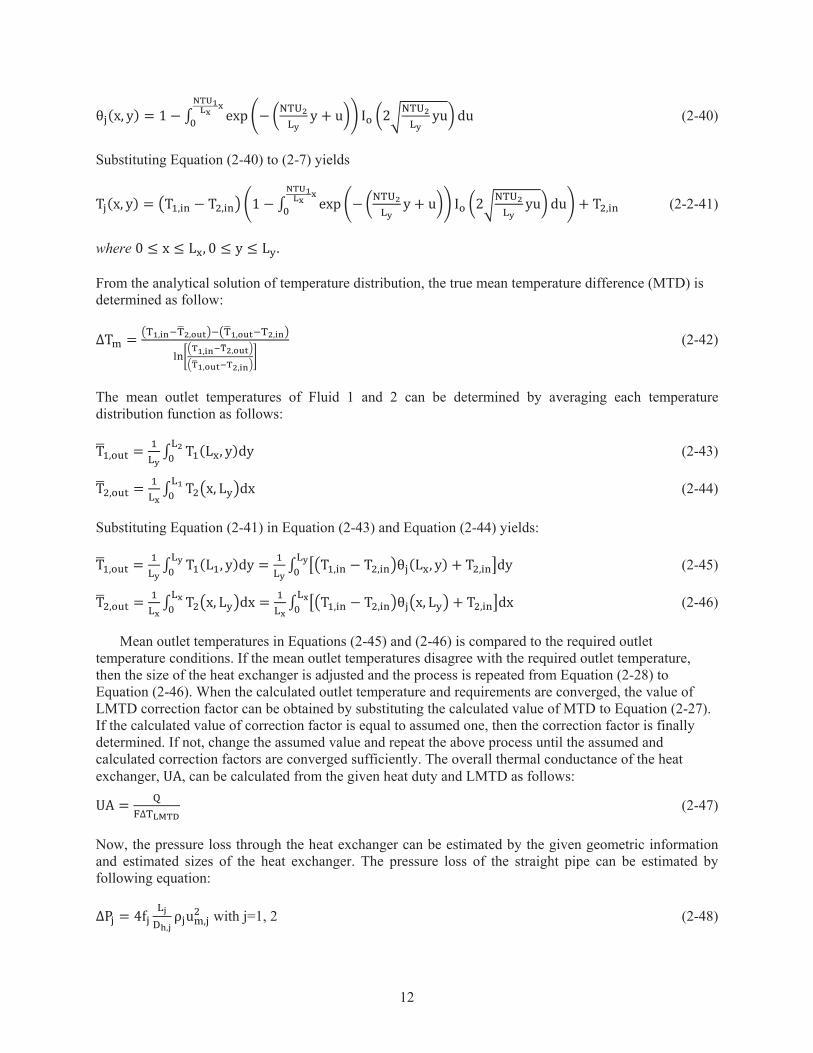
12

(2-40)

Substituting Equation (2-40) to (2-7) yields

(2-2-41)

where

From the analytical solution of temperature distribution, the true mean temperature difference (MTD) is determined as follow:

(2-42)

The mean outlet temperatures of Fluid 1 and 2 can be determined by averaging each temperature distribution function as follows:

(2-43)

(2-44)

Substituting Equation (2-41) in Equation (2-43) and Equation (2-44) yields:

(2-45)

(2-46)

Mean outlet temperatures in Equations (2-45) and (2-46) is compared to the required outlet temperature conditions. If the mean outlet temperatures disagree with the required outlet temperature, then the size of the heat exchanger is adjusted and the process is repeated from Equation (2-28) to Equation (2-46). When the calculated outlet temperature and requirements are converged, the value of LMTD correction factor can be obtained by substituting the calculated value of MTD to Equation (2-27). If the calculated value of correction factor is equal to assumed one, then the correction factor is finally determined. If not, change the assumed value and repeat the above process until the assumed and calculated correction factors are converged sufficiently. The overall thermal conductance of the heat exchanger, , can be calculated from the given heat duty and LMTD as follows:

(2-47)

Now, the pressure loss through the heat exchanger can be estimated by the given geometric information and estimated sizes of the heat exchanger. The pressure loss of the straight pipe can be estimated by following equation:

with j=1, 2 (2-48)

13

where

= pressure drop

= friction factor

L = length of channel

= hydraulic diameter of the channel

= mean flow velocity in the channel

j = index of fluid side.

Since the channel shape of PCHE is a semicircle, the pressure loss calculation using the friction factor correlation for a circular pipe can lead to an incorrect result. The flow channel of typical PCHE manufactured by Heatric is wavy (zigzag shaped). If the flow channel is wavy or zigzag shaped, the correlations for wavy or zigzag shaped channel should be employed. However, the straight pipe is assumed in this study so that the friction factor correlation by Berbish et al. [23] is employed to calculate the turbulent friction factor of semicircular straight pipe. The fully developed laminar friction factor [33] and turbulent friction factor of semicircular straight pipe are given by:

(2-49)

2.1.4 Mechanical Design of Crossflow Printed-Circuit Heat Exchanger To prevent the mechanical failure of the heat exchanger, the dimensions of the channel pitch and the

plate thickness should be larger than design criteria. The stress for both the plate-fin (PFHE) and printed-circuit heat exchangers (PCHE) is given by [33]:

(2-50)

where

= the absolute value of pressure difference between the two fluids

= is fin density

= is fin thickness.

The fin thickness in PFHE means the wall thickness between the flow channels in PCHE, since PCHE does not have typical fins. Equation (2-50) gives a maximum allowable pressure difference between the hot and cold fluid sides since the stress in Equation (2-50) should be lower than allowable stress of the structure. In order words, this equation gives the criterion of the minimum wall thickness for a given pressure difference. Thus, the minimum wall thickness is given by:

(2-51)

The fin density in PCHE, which is the number of channel walls per meter, is given by:

with j=1,2 (2-52)

14

The above fin density can be approximately expressed as a function of pitch as follow:

(2-53)

Therefore, the minimum wall thickness between the channels can be approximated as [34]:

(2-54)

Thus, the minimum pitch (P) of the channels can be calculated as:

(2-55)

In the PCHE, the plate can be assumed to be a thick-walled cylinder with an inner radius of D/2 and the outer radius of . Thus, the thickness of the plate [34] can be estimated by:

(2-56)

2.2 Thermal and Mechanical Design of Parallel/ Counter Flow Printed-Circuit Heat Exchanger

2.2.1 Analytical Modeling of Parallel/Counter Flow Printed-Circuit Heat Exchanger

Figure 10 shows the schematic diagram of channel configuration and arrangement of the parallel/counter flow PCHE. The definitions of the terms in the parallel/counter flow PCHE and the crossflow PCHE are basically the same.

Figure 10. Channel configuration and arrangement of PCHE.

15

Figure 11 shows the schematic diagram of energy balance of counter flow PCHE. The energy balance of the parallel flow PCHE is basically the same as the counter flow-type flow.

Figure 11. Energy balance of counter flow heat exchanger [21].

The energy balance equations in Equations (2-1)–(2-3) can be applied to the parallel/counter flow PCHE in the same manner. Thus, the energy balance equations of parallel/counter flow PCHE [21] are given by:

Fluid 1:

(2-57)

Fluid 2:

(2-58)

where is +1 or -1 for the same or opposite direction of the fluid 1 with respect to the positive direction of the x axis, respectively. In the same manner, is +1 or -1 for the same or opposite direction of the fluid 2, respectively, with respect to the positive direction of the x-axis.

If it is assumed that the distribution of the total heat transfer surface area along the channel length is uniform, a differential term is equal to . Thus, Equations (2-57) and (2-58) can be simplified as:

(2-59)

(2-60)

xT1,in

Th,out

T2,out T2,in

(mcp)2 = C2.

(mcp)1 = C1.T1

Heat transfer area Ax

q”

w

R=U-1 (= unit overall resistance)

dq

x

dA

C2T2

C1T1

Wall

x

C1(T1 + x)dT1dx

Cc(T2 + x)dT2dx

T2

16

To make a dimensionless form of above equations, the following dimensionless variables are defined by:

(Dimensionless temperature) (2-61)

(Dimensionless distance) (2-62)

Heat Capacity Rate Ratio is defined by:

(2-63)

The boundary conditions are given by:

(2-64)

(2-65)

Using the dimensionless variables from Equations (2-61) and (2-62) and NTU definition from Equation (2-39), the dimensionless forms of Equations (2-59) and (2-60) can be written as:

(2-66)

(2-67)

The dimensionless boundary conditions are given by:

(2-68)

(2-69)

2.2.2 Analytical Solution of Parallel/Counter Flow Printed-Circuit Heat Exchanger

The general solutions of the dimensionless temperature of parallel and counter flow PCHEs can be obtained by the Laplace transform method. The detailed solving procedure of the parallel/counter flow PCHE is similar to that of crossflow HX. The solution of each flow arrangement [21] is given by:

Parallel flow:

(2-70)

(2-71)

17

Counter flow:

(2-72)

(2-73)

2.2.3 Thermal Design of Parallel/Counter Flow Printed-Circuit Heat Exchanger Basically, the thermal design process of parallel/counter flow PCHE is similar to that of crossflow

PCHE. However, the overall heat transfer coefficient is obtained from the thermal resistance circuit shown in Figure 11 as follows:

(2-74)

where and are the heat transfer coefficients of Fluid 1 and 2 sides, respectively, and is the thermal resistance of the wall.

The mass flow rate through each fluid side can be obtained by Equation (2-24). The fluid velocity of each fluid side is calculated as follows:

with j=1, 2 (2-75)

where is total cross-sectional area of the fluid j.

The Reynolds number and Prandtl number of each fluid side are calculated as follows:

with j=1, 2 (2-76)

with j=1, 2 (2-77)

where

= thermal conductivity of the fluid j

= hydraulic diameter of fluid j side.

If the channel is assumed to be straight through the flow paths, the heat transfer can be estimated by the following heat transfer correlations [35]:

with j=1, 2 (2-78)

18

From the above Nusselt number correlation, the heat transfer coefficient in each fluid side can be estimated as follow:

with j=1, 2 (2-79)

The LMTDs of the parallel and counter flow configuration can be estimated by:

(2-80)

The overall heat transfer surface area is calculated as follow:

(2-81)

Note that the LMTD correction factor F is 1 for both the parallel and counter flow heat exchangers.

The numbers of flow channel in each side is calculated as follow:

with j=1, 2 (2-82)

The heat exchanger channel length can be estimated as follow:

with j=1, 2 (2-83)

The friction factor and pressure drop in the parallel/counter flow PCHE can be estimated by the same method used in the crossflow heat exchanger. Equations (2-48) and (2-49) are applied to estimate the pressure drop and friction factor of the flow channel, respectively. The result of thermal design of parallel/counter flow PCHE is summarized in Appendix A.

2.2.4 Mechanical Design of Parallel/Counter Flow Printed-Circuit Heat Exchanger

The mechanical design methodology of the crossflow heat exchanger can be applied to the parallel/counter flow PCHE. Thus, Equations (2-54), (2-55), and (2-56) can be applied to determine the minimum values of wall thickness between the channels, pitch, and plate thickness, respectively. The result of mechanical design of parallel/counter flow PCHE is summarized in Appendix B.

19

3. THERMAL-HYDRAULIC ANALYSIS OF CROSSFLOW PCHE Thermal design of heat exchanger is carried out to determine the size of heat exchanger that would

provide us the needed temperature at the outlet for the given inlet condition. This report focuses on the thermal-hydraulic analysis of crossflow PCHE. Temperature profile of parallel and counter flow PCHE is provided in Appendix A. The basic input parameters of PCHE used in this analysis is summarized in Table 3. Table 4 describes the typical temperature and pressure conditions of advanced small modular reactors (SMRs) according to the reactor coolants. Inlet and outlet temperatures of primary and secondary sides are determined based on the intermediate heat exchanger. Thus, the inlet temperature of the primary side shown in Table 4 is actually the outlet temperature of the reactor core. Thermal-hydraulic analysis of crossflow PCHE was carried out based on the values in Tables 3 and 4.

Table 3. Basic design parameters of PCHE. Geometric Parameters Value

Channel diameter , (m) 0.003 Channel pitch , (m) 0.0033 Plate thickness , (m) 0.00317 Fin thickness, tf, (m) 0.00013

Table 4. Typical temperature and pressure condition of heat exchanger for advanced SMRs.

Coolant Type

Coolants Operation Conditions

Primary/Secondary

Inlet/Outlet Temperature (°C)

Primary/Secondary Pressure (MPa) Primary Secondary

Water-cooled [36] Water/Water 323/295 200/293 15.0/5.0 Gas-cooled [37] He/He 950/637 351/925 7.0/7.0 Liquid Metal-cooled [38] Na/Na 545/390 320/526 0.1/0.1 Molten Salt-cooled [39] FLiBe/FLiNaK 700/650 600/690 0.1/0.1

3.1 Grid Sensitivity Test In this study, the temperature profile of crossflow PCHE is obtained by solving the system of

differential equations as described in Section 2. Since the temperature profile of crossflow PCHE is two-dimensional, two-dimensional grid are required to analyze the crossflow PCHE. In numerical simulation, the result is generally influenced by the grid. Thus, the outlet temperature of each channel can be varied due to the number of grid. In developed code, the mean outlet temperature of each fluid side is calculated by averaging the temperature at the outlet. Consequently, the number of grids can influence the mean outlet temperature. To investigate the grid effect, the grid sensitivity test was performed. Tested numbers of grid and results are summarized in Table 5. In grid sensitivity test, x and y-axial dimensions of heat exchanger, NTUs of primary and secondary sides are assumed to be a unity. The size of reference grid was 40 × 40.

Table 5. Grid sensitivity test results. Dimensionless Mean Outlet Temperature Numbers of Grids 5 × 5 10 × 10 20 × 20 40 × 40 80 × 80 160 × 160 320 × 320 Primary Side 0.52124 0.52251 0.52314 0.52346 0.52362 0.52370 0.52374 Secondary Side 0.47876 0.47749 0.47686 0.47654 0.47638 0.47630 0.47626

20

The grid sensitivity analysis by the Richardson extrapolation [40] was performed to estimate the numerical error due to the grid number. The approximation of exact solution is given by:

(3-1)

where is a numerical solution and the order of the scheme is defined by:

(3-2)

Figure 12 shows the dimensionless mean outlet temperatures of the primary and secondary sides. The dimensionless temperature in the grid sensitivity test was defined in Equation (2-7). The Richardson solutions of primary and secondary fluids were 0.5238 and 0.4762, respectively. The maximum relative errors between the reference grid (40 × 40) and Richardson solution of primary and secondary fluids were 0.48% and 0.53%, respectively. Consequently, the grid sensitivity test results show that the effect of grid number is negligible.

Figure 12. Effect of grid number on dimensionless mean temperature profile of crossflow heat exchanger.

3.2 Effectiveness-NTU ( -NTU) Method Analysis The effectiveness of the heat exchanger, , is the ratio of the actual heat transfer rate to the maximum

possible heat transfer rate of the exchanger and is defined by:

(3-3)

The -NTU method [10] is one of general methods applied for the thermal design of heat exchanger. In this method, the effectiveness of crossflow heat exchanger is a function of NTU. The relationship between the effectiveness and NTU of both unmixed fluids crossflow heat exchanger [41] is given by:

(3-4)

where is the ratio of minimum to maximum heat capacity rate of fluid.

The effectiveness of crossflow PCHE calculated by the developed code is compared with that of the -NTU method. Figure 13 shows the effectiveness-NTU plots by the developed code and -NTU method.

The effectiveness of a heat exchanger increases as the NTU increases. The effectiveness increases rapidly as the ratio of heat capacity rate decreases.

0 40 80 120 160 200 240 280 3200.517

0.518

0.519

0.520

0.521

0.522

0.523

0.524

secondary=0.4762

Dim

ensi

onle

ss m

ean

outle

t tem

pera

ture

of

sec

onda

ry fl

uid

Dim

ensi

onle

ss m

ean

outle

t tem

pera

ture

of

prim

ary

fluid

Number of grids

Primary Secondary

primary=0.5238

0.476

0.477

0.478

0.479

0.480

0.481

0.482

0.483

21

Figure 13. Effectiveness-NTU comparison between -NTU method and crossflow PCHE analysis code.

3.3 Effect of Fluid Property Uncertainty The uncertainty of fluid property can be propagated into the calculated temperature profile of the heat

exchanger. To evaluate the effect of uncertainty of fluid property, the uncertainty of fluid property was assumed to be ±30%. In this sensitivity test, the fluid properties in both primary and secondary side are changed at the same time. Tested variables are thermal conductivity, heat capacity and viscosity. In this calculation, the heat duty, the temperatures, and the pressures in Table 4 were employed. Hastelloy N is employed as the structural material. Gnielinski heat transfer correlation was used to calculate the heat transfer coefficient. The dimensions in x, y, and z axial directions of heat exchanger were assumed to be 0.9897 m, 0.9897 m, and 0.634 m, respectively. Corresponding numbers of flow channels are 300, 300, and 100, respectively.

Figures 14–21 show the average temperature profiles according to the uncertainty of thermo-physical property for each coolant. The density change did not have an effect on the temperature profile. In the developed code, when the heat duty is given, the mass flow rate is determined from Equation (2-24). Then, the density is used to calculate the fluid velocity and Reynolds number. Since the product of density and fluid velocity is constant by Equation (2-33), the Reynolds number is not changed by the density. Consequently, the uncertainty of fluid density does not have an effect on the temperature. Uncertainties of heat capacity and dynamic viscosity resulted in the same temperature profile. The temperature profile of the crossflow analytical model is determined by the size of heat exchanger and NTU value. In this crossflow model, NTU can be approximated as a function of the product of heat capacity and dynamic viscosity so that the changes of these two parameters resulted in the same value of NTU. Uncertainty of thermal conductivity led to the maximum deviation of temperature profile except the sodium case. The effect of thermal conductivity was relatively smaller than heat capacity and dynamic viscosity for the fluid of low Prandtl number. Overall, the relative deviation of the temperature profile according to the uncertainty of fluid property was very small. Maximum deviation was 2.38%, which occurred by the thermal conductivity in the primary side of helium flow. Consequently, it is concluded that the effect of fluid property on the analytical solution of crossflow heat exchanger was not as critical as expected.

0 1 2 3 4 5 6 7 8 9 100.0

0.1

0.2

0.3

0.4

0.5

0.6

0.7

0.8

0.9

1.0

1.1

Effe

ctiv

enes

sNTU

-NTU method PCHE analysis code C*=0.1 C*=0.1 C*=0.3 C*=0.3 C*=0.5 C*=0.5 C*=0.7 C*=0.7 C*=1 C*=1

22

Figure 14. Average temperature profile of primary fluid according to uncertainty of material property (Water).

Figure 15. Average temperature profile of secondary fluid according to uncertainty of material property (Water).

Figure 16. Average temperature profile of primary fluid according to uncertainty of material property (Helium).

0.0 0.2 0.4 0.6 0.8 1.0260

270

280

290

300

310

320

-0.47%

Aver

aged

tem

pera

ture

(o C)

Distance from the inlet (m)

k (-30%) cp(-30%) (-30%) Reference k (+30%) cp(+30%) (+30%)

+0.75%

0.0 0.2 0.4 0.6 0.8 1.0200

210

220

230

240

250

260

Ave

rage

d te

mpe

ratu

re (o C

)



+0.48%

-0.77%

0.0 0.2 0.4 0.6 0.8 1.0500

550

600

650

700

750

800

850

900

950

Aver

aged

tem

pera

ture

(o C)



+2.38%

-1.52%

23

Figure 17. Average temperature profile of secondary fluid according to uncertainty of material property (Helium).

Figure 18. Average temperature profile in primary side according to uncertainty of material property (Sodium).

Figure 19. Average temperature profile in secondary side according to uncertainty of material property (Sodium).

0.0 0.2 0.4 0.6 0.8 1.0350

400

450

500

550

600

650

700

750

800

Ave

rage

d te

mpe

ratu

re (o C

)


Reference k (-30%) cp(-30%) (-30%) k (+30%) cp(+30%) (+30%)

+1.05%

-1.65%

0.0 0.2 0.4 0.6 0.8 1.0360

380

400

420

440

460

480

500

520

540

560

Ave

rage

d te

mpe

ratu

re (o C

)



+0.7%

-0.47%

0.0 0.2 0.4 0.6 0.8 1.0320

340

360

380

400

420

440

460

480

500

Ave

rage

d te

mpe

ratu

re (o C

)



-0.54%

+0.37%

24

Figure 20. Average temperature profile in primary side according to uncertainty of material property (FLiBe).

Figure 21. Average temperature profile in secondary side according to uncertainty of material property (FLiNaK).

3.4 Effect of Heat Transfer Coefficient Correlations Comparative analyses were carried out to evaluate the effect of heat transfer correlations on the

temperature profile. In this analysis, the heat duty, the temperatures and pressures in Table 4 were employed. Hastelloy N was employed as the structural material. The number of channel in x, y and z axial directions were assumed to be 300, 300 and 100, and corresponding dimensions are 0.9897 m, 0.9897 m, and 0.634 m, respectively.

Figures 22 and 23 show the temperature profiles in the primary and secondary side with water as coolant, respectively. The Lubarsky and Kaufman’s correlation showed the highest temperature of primary side and lowest temperature of secondary side. Wu and Little’s and Kim et al.’s correlations showed the lowest temperature of primary side and highest temperature of secondary side. These two correlations predicted the heat transfer coefficients similarly for Prandtl number in the range of 0.5~1.0. Thus, the same temperature profile trend was observed in the water and helium flows of which Prandtl numbers were approximately 1.0 and 0.66, respectively. The maximum deviation among the averaged outlet temperature was 39.45 K, which was caused by the Lubarsky and Kaufman’s correlation and Kim et al.’s correlation. Figures 24 and 25 show the temperature profiles with helium flows which showed

0.0 0.2 0.4 0.6 0.8 1.0650

660

670

680

690

700

-0.51%

Ave

rage

d te

mpe

ratu

re (o C

)



+0.62%

0.0 0.2 0.4 0.6 0.8 1.0600

610

620

630

640

650

-0.64%

Ave

rage

d te

mpe

ratu

re (o C

)


Reference k (-30%) cp(-30%) (-30%) k (+30%) cp(+30%) (+30%)

+0.53%

25

similar trends as observed in the case with water. The maximum deviation among the averaged outlet temperature was approximately 196.01 K, which was caused by the Lubarsky and Kaufman’s correlation and Kim et al.’s correlation.

Figures 26 and 27 show the temperature profiles with sodium. In this case, the effect of heat transfer correlation was smaller than the other cases. For the fluids with very low Prandtl numbers, most of empirical correlations predicted a low-heat transfer coefficient, and the difference between them was also small. Maximum deviation of averaged outlet temperature was 15.34 K, which was caused by Gnielinski’s correlation and Kim et al.’s correlation. Figures 28 and 29 show the temperature profiles of molten salt flows. The Prandtl number for molten salt is approximately 10.0. Contrary to the sodium flow, the molten salt is a fluid with a high Prandtl number. Not only the empirical correlations developed for liquid metals but also Dittus-Boelter correlation and Gnielinski’s correlations predicted a higher heat transfer coefficient. Consequently, these correlations predicted similar temperature profiles. Maximum deviation of averaged outlet temperature was 31.04 K, by using Wang and Peng’s correlation and Lyon’s correlation.

By comparing heat transfer correlations for each fluid, it is found that the effect of heat transfer correlations was largest in the helium flow. The deviation of temperature profiles by the heat transfer correlation decreased for very low or very high Prandtl number fluids. It was not easy to determine a heat transfer correlation that can be applied generally irrespective of coolant types. Consequently, the experimental and computational validations are deemed to be required for the design of crossflow PCHE. In addition, the appropriate heat transfer correlation for each fluid type should be applied.

Figure 22. Temperature profile in primary side by the heat transfer correlations (Water).

Figure 23. Temperature profile in secondary side by the heat transfer correlations (Water).

0.0 0.2 0.4 0.6 0.8 1.0240

270

300

330

360

Wang and Peng

Wu and Little, Kim et al.

Ave

rage

tem

pera

tre (o C

)

Distrance from the Inlet (m)

Gnielinski Berbish Dittus-Boelter Kim et al Lyon Lubarsky and Kaufman Reed Taylor and Kirchgessner, Wieland Wu and Little Wang and Peng

Lubarsky and Kaufman

T=39 K

0.0 0.2 0.4 0.6 0.8 1.0200

220

240

260

280

Ave

rage

tem

pera

tre (o C

)



Wu and Little, Kim et al.

Wang and Peng


T=39 K

26

Figure 24. Temperature profile in primary side by the heat transfer correlations (Helium).

Figure 25. Temperature profile in secondary side by the heat transfer correlations (Helium).

Figure 26. Temperature profile in primary side by the heat transfer correlations (Sodium).

0.0 0.2 0.4 0.6 0.8 1.0400

500

600

700

800

900

1000

Kim et al.

Wang and Peng


Aver

age

tem

pera

tre (o C

)



Wu and Little

T=196 K

0.0 0.2 0.4 0.6 0.8 1.0

400

500

600

700

800

900

Aver

age

tem

pera

tre (o C

)




Wang and Peng

Wu and Little

Kim et al.

T=196 K

0.0 0.2 0.4 0.6 0.8 1.0350

400

450

500

550

Ave

rage

tem

pera

tre (o C

)



Gnielinski

Berbish, Wu and Little, and Kim et al. T=15 K

27

Figure 27. Temperature profile in secondary side by the heat transfer correlations (Sodium).

Figure 28. Temperature profile in primary side by the heat transfer correlations (Molten Salt).

Figure 29. Temperature profile in secondary side by the heat transfer correlations (Molten Salt).

0.0 0.2 0.4 0.6 0.8 1.0300

350

400

450

500

550

Gnielinski

Berbish, Wu and Little, and Kim et al.

Ave

rage

tem

pera

tre (o C

)



T=15 K

0.0 0.2 0.4 0.6 0.8 1.0620

640

660

680

700

720

Lyon

Ave

rage

tem

pera

tre (o C

)



Wang and Peng

T=31 K

0.0 0.2 0.4 0.6 0.8 1.0560

580

600

620

640

660

Ave

rage

tem

pera

tre (o C

)



T=31 K

Wang and Peng

Lyon

28

4. MECHANICAL DESIGN OF CROSSFLOW PCHEs The assumptions and basic parameters of crossflow PCHE for mechanical design are summarized in

Table 6.

Table 6. Assumptions and basic parameters of crossflow PCHE for mechanical design. Parameter Water/Water Sodium/Sodium M-S/M-S He/He

Primary side pressure(Pp), (Pa) 1.5 × 107 1.01 × 105 1.01 × 105 7.0 × 106 Secondary side pressure(Ps), (Pa) 5.0 × 106 1.01 × 105 1.01 × 105 7.0 × 106 Channel diameter (D), (m) 0.003 Channel pitch (P), (m) 0.0033 Plate thickness (tp), (m) 0.00317 Maximum allowable stress( max), (Pa) 2.18 × 108

Equations (2-55) and (2-56) are applied to determine the minimum values of pitch of channels and

plate thickness, respectively. Calculated pitch of channels and plate thickness of each coolant are summarized in Table 7. The calculated pitch of channels and plate thickness of each coolant satisfied the criteria of mechanical design.

Table 7. Calculated pitch of channels and plate thickness of each coolant. Parameter Water/Water Sodium/Sodium M-S/M-S He/He

Channel pitch (P), (m) 0.0031 0.003 0.003 0.003 Plate thickness (tp), (m) 0.0016 0.0015 0.0015 0.0015

29

5. ECONOMIC ANALYSIS OF CROSSFLOW PCHEs 5.1 Cost Estimation Method

The cost of heat exchanger is one of the important factors for development of heat exchanger. The total cost of a heat exchanger consists of capital cost and operating cost. The capital cost is related to the material cost of the heat exchanger so that it can be estimated based on its weight. Therefore, the capital cost depends on the structural material and size of the heat exchanger. The total mass of heat exchanger is given by:

(5-1)

The volume of the heat exchanger can be approximated as follow:

(5-2)

The capital cost (CP) can be calculated by multiplying the cost factor of material (CM) and the total mass of heat exchanger (MHX) as follow:

(5-3)

On the other hand, the operating cost is estimated based on the thermal hydraulic condition of the heat exchanger. Since the operating cost is defined as the cost to operate the circulation pump of the heat exchanger, it is important to optimize the design of heat exchanger to reduce the pressure loss, and in turn, reducing the operating cost. To estimate the operating cost, the pumping power of the heat exchanger is used. The pumping powers of the heat exchanger in hot and cold fluid sides can be defined by [8]:

(5-4)

(5-5)

where

= is a mass flow rate

= pressure loss, and is a density of fluid.

Thus, the operating cost can be approximated as follow [8]:

(5-6)

where

= cost per time (e.g., electricity cost per time)

= the total duration of operation.

Therefore, the total cost of heat exchanger becomes:

(5-7)

30

5.2 Results of Economic Analysis In this crossflow PCHE analysis code, the size of heat exchanger is determined by iterative

calculation to meet the given heat duty and temperature requirements. In this economic analysis, the heat duty and temperature requirements as shown in Table 4 and three nickel based structural alloys as shown in Table 1 were used. The maximum operating period of heat exchanger is assumed to be 20 years. In this analysis, the height of heat exchanger, Lz, was fixed to 0.634 m to reduce the number of cases. If the height of the heat exchanger can be varied, the length and width of the heat exchanger are determined for each height so that various heat exchanger sizes can be generated. Economic analysis results are summarized in Table 8. For the given requirements of each coolant, the size of heat exchanger, average outlet temperature, capital cost and operation cost were determined.

Table 8. The result of economic analysis of crossflow PCHE.

Coolants

Heat exchanger size (m)

Average outlet temperature( C)

Cost, (USD) (Operation period: 20 year)

Primary Secondary Structural Material Capital Operation

Water 0.396 1.518

0.634

295.3 293.6 Alloy 617 3.82·105 1.40·109 Alloy 800H 3.62·105 1.44·109 Hastelloy N 4.18·105 1.41·109

Helium 1.128 2.095 637.8 925.3 Alloy 617 1.50·106 9.48·109 Alloy 800H 1.43·106 9.49·109 Hastelloy N 1.65·106 9.48·109

Sodium 1.214 1.613 390.2 526.0 Alloy 617 1.25·106 1.27·108 Alloy 800H 1.18·106 1.28·108 Hastelloy N 1.36·106 1.27·108

Molten Salt 6.352 11.880 651.0 690.2

Alloy 617 4.80·107 9.12·106 Alloy 800H 4.56·107 9.12·106 Hastelloy N 5.26·107 9.12·106

The capital cost of crossflow PCHE was relatively smaller than the operation cost except for molten salt heat exchanger. Due to the large size of the molten salt heat exchanger, its capital cost was estimated to be larger than operation cost. The capital cost of the molten salt heat exchanger was higher than the others, but the operation cost was much lower. The operation cost of the helium heat exchanger was the highest. Figures 30–33 show the total cost per year of the heat exchangers according to the operation period. Operation cost per year decreased as the operation period increased. Total cost of the heat exchanger using Alloy 617 was cheaper than the other structural materials except for the molten salt heat exchanger. In the molten salt heat exchanger, the total cost was minimized by using Alloy 800H. The total cost per year of molten salt heat exchanger decreased rapidly as the operation period increased.

31

Figure 30. Total cost per year of crossflow PCHE (Water/Water).

Figure 31. Total cost per year of crossflow PCHE (Helium/Helium).

Figure 32. Total cost per year of crossflow PCHE (Sodium/Sodium).

3 6 9 12 15 18 217E6

7.05E6

7.1E6

7.15E6

7.2E6

7.25E6

7.3E6

7.35E6

7.4E6

Tota

l cos

t per

yea

r (U

SD

/yr)

Operation period (yr)

Alloy 617 Alloy 800H Hastelloy N

3 6 9 12 15 18 21

4.737E8

4.74E8

4.743E8

4.746E8

4.749E8

4.752E8

4.755E8

Tota

l cos

t per

yea

r (U

SD

/yr)



3 6 9 12 15 18 216.3E6

6.4E6

6.5E6

6.6E6

6.7E6

6.8E6

Tota

l cos

t per

yea

r (U

SD

/yr)



32

Figure 33. Total cost per year of crossflow PCHE (FLiBe/FLiNaK).

3 6 9 12 15 18 212E6

4E6

6E6

8E6

1E7

1.2E7

Tota

l cos

t per

yea

r (U

SD/y

r)



33

6. CONCLUSION In this study, the methodologies for thermal and mechanical designs of printed circuit heat exchanger

with parallel, counter, and crossflow configuration were reported. The analytical solutions for temperature profiles in primary and secondary sides were described for each flow configuration. This work focused on the crossflow PCHE because parallel and counter flow PCHEs were studied previously (INL/EXT-11-23076). Thus, in this study, the crossflow PCHE analysis code has been developed to evaluate the size and cost of heat exchangers by implementing the analytical solution of single pass, both unmixed fluids crossflow heat exchanger model. Two-dimensional temperature distribution of crossflow PCHE was calculated by the analytical solution. General methods for thermal design and cost estimation of heat exchangers were employed to determine the size and cost of heat exchanger, respectively.

The grid sensitivity test of the code showed that the effect of grid on the temperature profile was negligible. The effectiveness calculated by the code showed a good agreement with that by well-known -NTU method. The uncertainty of fluid property was propagated into the temperature distribution, but its

effect was small enough to be inconsequential. The heat transfer correlations had a considerable influence on the temperature profile. The temperature profile of crossflow PCHE using helium gases showed the largest deviation by the heat transfer correlations. The deviation of temperature profiles by the heat transfer correlation decreased for a very low or a very high Prandtl number of fluids. However, it was not easy to determine the most accurate heat transfer correlation for the heat exchangers using various combinations of coolants. Consequently, experimental and computational validations are required to determine the best heat transfer correlation for each coolant.

Costs of crossflow PCHE for the high temperature reactor designs were investigated. Capital costs of PCHE for water, helium, and sodium flows were lower than their operation costs, whereas capital cost of molten salt heat exchanger was higher than its operation cost. Total cost of heat exchanger using Alloy 617 was cheaper than the other structural materials except for the molten salt heat exchanger. In the molten salt heat exchanger, the total cost was minimized by using Alloy 800H, and in future potential Hastelloy N linear could be used to enhance corrosion resistance.

34

7. REFERENCES 1. Hewitt, G. F., Shires, G. L., Bott, T. R., Process Heat Transfer, CRC Press, Boca Raton, Florida,

1994.

2. Shah, R. K., Willmott, A. J., Thermal Energy Storage and Regeneration, Hemisphere/McGraw-Hill, Washington, DC, 1981.

3. AWs, Diffusion Welding and Diffusion Brazing, Chapter 12, pp. 437–442, Welding Handbook, 9th Ed., American Welding Society, 2007.

4. Sabharwall, P., E. S. Kim, A. Siahpush, N. Anderson, M. Glazoff, B. Phoenix, R. Mizia, D. Clark, M. McKellar, M.W. Patterson, “Feasibility Study of Secondary Heat Exchanger Concepts for the Advanced High Temperature Reactor,” INL/EXT-11-23076, 2011.

5. Heatric Homepage, Available online at http://www.heatric.com, accessed April 16, 2013.

6. Grady, C., “PCHE – Printed Circuit Heat Exchangers,” Presentation at the Heatric Workshop at MIT on 2nd October 2003, Cambridge: MA, 2003.

7. Southall, D., “Diffusion Bonding in Compact Heat Exchangers,” Proceeding of ICAPP’09, Tokyo, Japan, May 10–14, 2009.

8. Kim, E. S., C. H. Oh, S. Sherman, “Simplified Optimum Sizing and Cost Analysis for Compact Heat Exchanger in VHTR,” Nuclear Engineering and Design, Vol. 238, pp. 2635–2647, 2008.

9. Kim, I. H., “Experimental and numerical investigations of thermal-hydraulic characteristics for the design of a Printed Circuit Heat Exchanger (PCHE) in HTGRs,” Ph.D. Thesis, KAIST, 2012.

10. Nusselt, W., “Der Warmeiibergang im Kreuzstrom,” Z. Ver.dt. Ing. 55, pp. 2021–2024, 1911.

11. Nusselt, W., “Eine neue Formel fur den Warmedurchgangim Kreuzstrom,” Tech. Mech. Thermo-Dynam., Berl. 1, pp. 417–422, 1930.

12. Smith, D. M., “Mean Temperature-difference in Cross Flow,” Engineering Vol.138, pp. 479–481 and pp. 606–607, 1934.

13. Binnie, A. M., and E. G. C. Poole, “The Theory of the Single Pass Cross-flow Heat Interchanger,” Proc. Cambr. Phil. Sot., 33, pp. 403–411, 1937.

14. Mason, J. L., Heat Transfer in Crossflow, Proc. Second U.S. National Congress of Applied Mechanics, American Society of Mechanical Engineers, New York, pp. 801–803, 1955.

15. Kiihl, H., Probleme des Kreuzstrom- Warmeaustauschers, Springer, Berlin, 1959.

16. Schedwill, H., “Termische Auslegung von Kreuzstromwarmeaustauchern,” Fortsch.-Ber. VDI-Z, Reihe 6, Nr.19, 1968.

17. Ishimaru,T., N. Kokubo, and R. Izumi, “Performance of Crossflow Heat Exchanger,” Bull. Jup. Soc. mech. Engrs, 19, pp. 1336–1343, 1976.

18. Romie, F. E., “Transient Response of Gas-to-gas Crossflow Heat Exchangers with neither Gas Mixed,” Trans. Am. Sec. Mech. Engrs, J. Heat Transfer, 105, pp. 563–570, 1983.

19. Lach, J., “The Exact Solution of the Nusselt’s Model of the Cross-flow Recuperator,” Int. J. Heat Mass Transfer, 26, pp. 1597–1601, 1983.

20. Baclic, B. S., and P. J. Heggs, “On the Search for New Solutions of the Single-pass Crossflow Heat Exchanger Problem,” Int. J. Heat Mass Transfer. Vol. 28, No. 10, pp. 1965–1976, 1985.

35

21. Shah, R. K., D. P. Sekulic, Fundamentals of Heat Exchanger Design, John Wiley & Sons, Inc., Hoboken, New Jersey, 2003.

22. Welty, J. R., C. E. Wicks, R. E. Wilson, Fundamentals of Momentum, Heat, and Mass Transfer, John Wiley & Sons, 1984.

23. Berbish, N. S., M. Moawed, M. Ammar, R. I. Afifi, “Heat Transfer and Friction Factor of Turbulent Flow through a Horizontal Semi-circular Duct,” Heat and Mass Transfer, Vol. 47, pp.377–384, 2011.

24. Kim, I. H., H. C. No, J. I. Lee, B. G. Jeon, “Thermal Hydraulic Performance Analysis of the Printed Circuit Heat Exchanger using a Helium Test Facility and CFD Simulations,” Nuclear Engineering and Design, Vol. 239, pp. 2399–2408, 2009.

25. Winterton, R. H. S., “Where did the Dittus-Boelter equation come from?,” International Journal of Heat and Mass Transfer, Vol. 41, Nos 4 5, pp. 809–810, 1998.

26. Gnielinski, V., “New Equation for Heat and Mass Transfer in Turbulent Pipe and Channel Flow,” International Chemical Engineering, Vol.16, pp. 359–368, 1976.

27. Lyon, R. N., Liquid Metal Heat Transfer Coefficients, Chemical Engineering Progress, Vol. 47, pp.75–79, 1951.

28. Lubarsky, B., S. J. Kaufman, “Review of Experimental Investigations of Liquid Metal Heat Transfer,” NACA Report 1270, Lewis Flight Propulsion Laboratory, 1956.

29. Kakac, S., R. K. Shah, W. Aung, Handbook of Single Phase Convective Heat Transfer, John Wiley & Sons, 1987.

30. Wieland, W. F., “Measurement of Local Heat Transfer Coefficients for Flow of Hydrogen and Helium in a Smooth Tube at High Surface to Fluid Bulk Temperature Ratios,” Paper Presented at AIChE Symposium on Nuclear Engineering Heat Transfer, Chicago, Ill., December 1962.

31. Wu, P., W. A. Little, “Measurement of the Heat Transfer Characteristics of Gas Flow in Fine Channel Heat Exchanger used for Microminiature Refrigerators,” Cryogenics, Vol. 24, Issue 8, pp. 415–420, 1984.

32. Wang, B. X., X. F. Peng, “Experimental Investigation on Liquid Forced Convection Heat Transfer through Microchannels,” International Journal of Heat and Mass Transfer, Vol. 37, Supplement 1, pp. 73–82, 1994.

33. Hesselgreaves, J. E., Compact Heat Exchangers: Selection, Design and Operation, Pergamon Press, 2001.

34. Oh, C. H., E. S. Kim, “Heat Exchanger Design Options and Tritium Transport Study for the VHTR System,” INL/EXT-08-14799, 2008.

35. Welty, J. R., C. E. Wicks, R. E. Wilson, Fundamentals of Momentum, Heat, and Mass Transfer, John Wiley & Sons, 1984.

36. Lee, Won Jae, “The SMART Reactor,” 4th Annual Asian Pacific Nuclear Energy Forum, June 18–19, 2010.

37. Richards, M., A. Shenoy, K. Schultz, L. Brown, E. Harvego, M. Jean Phillippe Coupey, S. M. Moshin Reza, F. Okamoto, “H2-MHR Conceptual Designs Based on the SI Process and HTE,” 3rd Information Exchange Meeting on Nuclear Production of Hydrogen and Second HTTR Workshop on Hydrogen Production Technologies, October 5–7, Japan Atomic Energy Research Institute, Oarai, Japan, 2005.

38. Hahn, Do Hee, et al., “Conceptual Design of the Sodium Cooled Fast Reactor KALIMER 600,” Nuclear Engineering and Technology, Vol. 39, No.3, pp. 193–206, 2007.

36

39. Greene, S. R., et al., “Pre Conceptual Design of a Fluoride Salt Cooled Small Module Advanced High Temperature Reactor (SmAHTR),” ORNL report, ORNL/TM 2010/199, 2010.

40. Richardson, L. F., “The Approximate Arithmetical Solution by Finite Differences of Physical Problems Involving Differential Equations, with an Application to the Stresses in a Masonry Dam,” Philos. Trans. Roy. Soc. London Ser. A, Vol. 210, pp. 307–357, 1910.

41. Triboix, A., “Exact and Approximate Formulas for Cross Flow Heat Exchangers with Unmixed Fluids,” International Communications in Heat and Mass Transfer, Vol.36, pp. 121–124, 2009.

37

Appendix A

Thermal Design of Parallel/Counter Flow PCHE Thermal design of parallel/counter flow PCHE was performed in previous study [4]. In this report,

thus, the results of previous study will be introduced.

Heat exchanger operating conditions are summarized in Table A-1.

Table A-1. Heat exchanger operating conditions. Parameters Primary Side Secondary Side

Heat Duty, MWth 3400 Fluid Material Molten Salt Steam/water Inlet Temperature, oC 679 251 Outlet Temperature, oC 587 593 Pressure, MPa 0.1 25

The geometric parameters of parallel/counter flow PCHE are summarized in Table A-2.

Table A-2. Basic geometry parameters of parallel/counter flow PCHE. Parameters Value

Channel Diameter, m 0.003 Channel Pitch, m 0.0033 Channel Thickness, m 0.00317 Channel Horizontal Distance, m 3×10-4 Surface Area Density, 1/m 737.252 Ratio of Free Flow Area to Frontal Area 0.338 Effective Diameter, m 1.833×10-3

The primary coolant was molten-salt (KF-ZrF4) and the secondary coolant was water/steam. The

basic properties of the coolants and structural material are summarized in Table A-3.

Table A-3. Thermo-physical properties of coolants.

Parameters Molten-Salt (KF-ZrF4)

Water (Average)

Density, kg/m3 2800 337 Thermal Conductivity, W/(m·K) 0.45 0.29 Heat Capacity, J/(kg·K) 1046.7 6510 Viscosity, Poise 0.051 5.23×10-4 Structural Material (Hastelloy N) Thermal Conductivity, W/(m·K) 23.5

38

The flow parameters for the parallel and counter flow PCHE are summarized in Table A-4. The values of flow parameters of parallel and counter flow PCHE are equal to each other.

Table A-4. Flow parameters of parallel and counter flow PCHE. Parameters Value

Mass Flow in the Primary Side (Hot Channel), kg/s 35307.65 Mass Flow in the Secondary Side (Cold Channel), kg/s 1640.89 Coolant Velocity in Primary Side, m/s 0.95 Coolant Velocity in Secondary Side, m/s 0.75 Reynolds Number in Primary Side 1020.57 Reynolds Number in Secondary Side 8764.60 Prandtl Number in Primary Side 11.35 Prandtl Number in Secondary Side 1.14 Nusselt Number in Primary Side 3.66 Nusselt Number in Secondary Side 34.52 Colburn Factor in Primary Side 1.59×10-3 Colburn Factor in Secondary Side 3.77×10-3

The overall heat transfer characteristics of parallel and counter flow PCHE are summarized in

Table A-5.

Table A-5. Overall heat transfer characteristics of parallel and counter flow PCHE. Parameters Value

Overall Heat Transfer Coefficient, W/(m2·K) 760.34 Heat Transfer Surface Area, m2 24375.31 Log Mean Temperature Difference, K 0.86 Heat Exchanger Channel Length, m 0.86

Figures A-1 and A-2 show the temperature profiles of parallel and counter flow PCHE.

Figure A-1. Temperature profile of parallel flow PCHE.

39

Figure A-2. Temperature profile of counter flow PCHE.

40

Appendix B

Mechanical Design of Parallel /Counter Flow PCHE The basic assumptions and input parameters of parallel and counter flow PCHEs are summarized in

Table B-1. The working fluids of primary and secondary sides in this analysis were molten salt and steam/water, respectively.

Table B-1. Assumptions and input parameters of parallel/counter flow PCHE for mechanical design. Parameter Value Note

Channel diameter (D), m 0.003 Assumption Channel pitch (P), m 0.0033 Assumption Plate thickness (tp), m 0.00317 Assumption Primary side pressure(Pp), Pa 2.5 × 107 Based on supercritical Rankine cycle Secondary side pressure(Ps), Pa 1.01 × 105 Based on molten salt intermediate loop Maximum allowable stress( max), Pa 2.18 × 108 Yield stress for Alloy N at 700°C

The pitch of the channels can be estimated by:

(B-1)

In the PCHE, the plate can be assumed to be a thick-walled cylinder with an inner radius of d/2 and an outer radius of tp. Therefore, the thickness of the plate, tp can be estimated by:

(B-2)

In conclusion, the assumed pitch of channels and plate thickness satisfied the criteria of mechanical design.

analytical study on thermal and mechanical design …/67531/metadc864854/m2/1/high...analytical...

Documents