analytical modeling and simulation of metal cutting … · shear zone model was revisited. a more...
TRANSCRIPT

ANALYTICAL MODELING AND SIMULATION OF
METAL CUTTING FORCES FOR ENGINEERING
ALLOYS
by
Lei Pang
A Thesis Submitted in Partial Fulfillment
of the Requirements for the Degree of
Doctor of Philosophy
in
The Faculty of Engineering and Applied Science
University of Ontario Institute of Technology
April 2012
© Lei Pang, 2012

i
ABSTRACT
In the current research, an analytical chip formation model and the methodology to
determine material flow data have been developed. The efforts have been made to
address work hardening and thermal softening effects and allow the material to flow
continuously through an opened-up deformation zone. Oxley's analysis of machining is
extended to the application of various engineering materials. The basic model is
extended to the simulation of end milling process and validated by comparing the
predictions with experimental data for AISI1045 steel and three other materials (AL-
6061, AL7075 and Ti-6Al-4V) from open literatures.
The thorough boundary conditions of the velocity field in the primary shear zone are
further identified and analyzed. Based on the detailed analysis on the boundary
conditions of the velocity and shear strain rate fields, the thick “equidistant parallel-sided”
shear zone model was revisited. A more realistic nonlinear shear strain rate distribution
has been proposed under the frame of non-equidistant primary shear zone configuration,
so that all the boundary conditions can be satisfied.
Based on the developed model, inverse analysis in conjugation of genetic algorithm
based searching scheme is developed to identify material flow stress data under the
condition of metal cutting.

ii
On the chip-tool interface, The chip-tool interface is assumed to consist of the secondary
shear zone and elastic friction zone(i.e. sticking zone and sliding zone). The normal
stress distribution over the entire contact length is represented by a power law equation,
in which the exponent is determined based on the force and moment equilibrium. The
shear stress distribution for the entire contact length is assumed to be independent of the
normal stress. The shear stress is assumed to be constant for the plastic contact region
and exponentially distributed over the elastic contact region, with the maximum equal to
the shear flow stress at the end of sticking zone and zero at the end of total contact. The
total contact length is derived as a function governed by the shape of normal stress
distribution. The length of the sticking zone is determined as the distance from the
cutting edge to the location where the local coefficient of friction reaches a critical value
that initiates the bulk yield of the chip. Considering the shape of the secondary shear
zone, the length of the sticking zone can also be determined by angle relations. The
maximum thickness of the secondary shear zone is determined by the equality of the
sticking lengths calculated by two means. With an arbitrary input of the sliding friction
coefficient, various processing parameters as well as contact stress distributions during
orthogonal metal cutting can be obtained.

iii
ACKNOWLEDGMENTS
I would like to express my sincere appreciation to my supervisor, Professor Hossam A.
Kishawy, not only for his brilliant guidance that all professors I believe are willing to
afford, but his always trust and care that make me fortunate to work under him as well.
My appreciation extends to Prof. D. Zhang, Prof. M. Hassan, Prof. A. Mohany and Prof.
H. Gabbar for being on my dissertation committee and providing valuable comments.

iv
TABLE OF CONTENTS
ABSTRACT………….. ...................................................................................................... i
ACKNOWLEDGMENTS ................................................................................................ iii
TABLE OF CONTENTS .................................................................................................. iv
LIST OF TABLES ..............................................................................................................x
LIST OF SYMBOLS ........................................................................................................ xi
CHAPTER 1. INTRODUCTION .....................................................................................1
1.1 Background ...............................................................................................1
1.2 Research objectives ...................................................................................3
1.3 Thesis outline ............................................................................................4
CHAPTER 2. LITERATURE REVIEW ..........................................................................7
2.1 Orthogonal and oblique cutting process ....................................................7
2.2 Thin shear plane models ..........................................................................10
2.3 Thick deformation zone models ..............................................................18
2.4 Oxley's predictive machining theory .......................................................25
CHAPTER 3. EXTENSION OF OXLEY'S MACHINING THEORY FOR VARIOUS
MATERIALS ..........................................................................................35
3.1 Introduction .............................................................................................35
3.2 Description of Johnson-Cook material model .........................................36

v
3.3 Generic constitutive equation based analysis ..........................................37
3.4 Conclusion ...............................................................................................44
CHAPTER 4. END MILLING SIMULATION .............................................................47
4.1 Introduction .............................................................................................47
4.2 Mechanics of milling process ..................................................................48
4.3 Geometry of milling process ...................................................................52
4.4 Mechanistic models for milling process ..................................................53
4.5 Analytical modeling of milling forces .....................................................59
4.5.1. Angular position ......................................................................................60
4.5.2. Chip load calculation ...............................................................................63
4.5.3. Entry and Exit angle ................................................................................68
4.5.4. Milling force prediction ...........................................................................71
4.5.5. Results and verification ...........................................................................79
4.6 Conclusion ...............................................................................................92
CHAPTER 5. PHENOMENOLOGICAL MODELING OF DEFORMATION
DURING METAL CUTTING ................................................................93
5.1 Introduction .............................................................................................93
5.2 Velocity, strain and strain rate during chip formation .............................94
5.3 Results and discussion ...........................................................................111
5.4 Conclusion .............................................................................................122

vi
CHAPTER 6. IDENTIFICATION OF MATERIAL CONSTITUTIVE EQUATION
FOR METAL CUTTING ......................................................................123
6.1 Introduction ...........................................................................................123
6.2 Inverse analysis in the primary shear zone ............................................126
6.3 Development of Genetic Algorithm for the system identification ........127
6.3.1. Encoding ................................................................................................128
6.3.2. Selection scheme ...................................................................................129
6.3.3. Mutation and crossover operator ...........................................................130
6.3.4. Terminating criteria ...............................................................................133
6.4 Results and discussions .........................................................................135
6.5 Conclusion .............................................................................................144
CHAPTER 7. TRIBOLOGICAL ANALYSIS AT THE CHIP-TOOL INTERFACE.145
7.1 Introduction ...........................................................................................145
7.2 Modeling dual zone chip-tool interface .................................................147
7.3 Results and discussion ...........................................................................155
7.4 Conclusion .............................................................................................157
CHAPTER 8. THESIS SUMMARY AND FUTURE WORK ....................................158
8.1 Thesis summary .....................................................................................158
8.2 Future work ...........................................................................................159
REFERENCES…………. ..............................................................................................161

vii
LIST OF FIGURES
Figure 2-1 Plastic deformation zones in metal cutting .......................................................8
Figure 2-2 Orthogonal metal cutting process......................................................................9
Figure 2-3 Oblique metal cutting process .........................................................................10
Figure 2-4 'Deck-of-Cards' chip formation model ............................................................11
Figure 2-5 Merchant's shear plane force circle .................................................................15
Figure 2-6 Lee and Shaffer's slipline filed model .............................................................17
Figure 2-7 Okushima and Hitomi's model ........................................................................20
Figure 2-8 Zorev's schematic representation of lines of slip in chip formation zone .......22
Figure 2-9 Oxley's shear zone model ................................................................................23
Figure 2-10 Simplified representation of parallel-sided deformation zones ....................27
Figure 3-1 The assumed curve of the main shear plane as a slipline ................................39
Figure 3-2 Forces acting on the chip as a free body .........................................................45
Figure 3-3 Flow chart of the methodology for the simulation of orthogonal cutting
process .............................................................................................................46
Figure 4-1 Up milling .......................................................................................................49
Figure 4-2 Down milling ..................................................................................................50
Figure 4-3 Face milling .....................................................................................................51
Figure 4-4 Semented milling tool model ..........................................................................60
Figure 4-5 Geometry of cutting tool .................................................................................62
Figure 4-6 Chipload in end milling ...................................................................................64
Figure 4-7 Radial offset runout of the milling cutter ........................................................66

viii
Figure 4-8 Chip thickness diagram during end milling[19] ..............................................67
Figure 4-9 Demonstration of immersion angles ...............................................................69
Figure 4-10 Immersion angles under the condition of runout ..........................................71
Figure 4-11 Conventional Oblique Cutting Forces ...........................................................72
Figure 4-12 Tube-end oblique cutting forces....................................................................75
Figure 4-13 Flow chart of analytical simulation of end milling process ..........................78
Figure 4-14 Comparison of predicted cutting forces based on Oxley‟s original model
with measured data for AISI 1045 ................................................................82
Figure 4-15 Comparison of predicted cutting forces based on modified Oxley‟s model
with measured data for AISI 1045 ................................................................84
Figure 4-16 Comparison of predicted cutting forces based on modified Oxley‟s model
with measured data for AL6061-T6 ..............................................................88
Figure 4-17 Comparison of predicted cutting forces based on modified Oxley‟s model
with measured data for Ti6Al4V ..................................................................89
Figure 4-18 Comparison of predicted cutting forces based on modified Oxley‟s model
with measured data for AL7075 ....................................................................90
Figure 5-1 Simplified non-equidistance primary shear zone ............................................95
Figure 5-2 Demonstration of the distribution of tangential velocity and shear strain rate
in the primary shear zone ..............................................................................102
Figure 5-3 Primary shear zone proportion ......................................................................107
Figure 5-4 Shear strain rate distribution through the primary shear zone ......................108
Figure 5-5 Tangential velocity distribution through the primary shear zone .................109
Figure 5-6 Shear strain distribution through the primary shear zone .............................110
Figure 5-7 Machining forces for 0.20% carbon steel: .................113

ix
Figure 5-8 Chip thickness for 0.20% carbon steel: ......................113
Figure 5-9 Predicted thickness and the proportion factor of the primary shear zone for
0.20% carbon steel: ..................................................114
Figure 5-10 Secondary shear zone thickness for 0.20% carbon steel: ............................117
Figure 5-11 Predicted shear strain rate, shear strain and velocity distributions across the
primary shear zone for 0.20% carbon steel:
..............................................................................................................119
Figure 5-12 Comparison of predicted machining forces with experimental data [38] for
AISI 1045 steel: .....................................................................121
Figure 6-1 Chromosome strings arrangement .................................................................128
Figure 6-2 Demonstration of multi-point mutation ........................................................132
Figure 6-3 Flow chart of identification of Johnson-Cook parameters using genetic
algorithm ........................................................................................................134
Figure 6-4 Error of the best result for each generation ...................................................136
Figure 6-5 Comparison of shear angle with the data used for system identification ......139
Figure 6-6 Comparison of cutting forces with data used for system identification ........140
Figure 6-7 Comparison of the cutting forces using GA determined JC parameters with
the experimental data from[38] ...................................................................143
Figure 7-1 Distribution of normal and shear stress at chip-tool interface ......................146
Figure 7-2 Triangular dual zone model ..........................................................................148
Figure 7-3 Flow chart of dual friction zone chip formation model ................................154
Figure 7-4 Comparison of cutting forces predicted by dual zone friction model ...........156

x
LIST OF TABLES
Table 4-1 Cutting conditions for end milling of AISI1045 ..............................................80
Table 4-2 Chemical composition of AISI1045 .................................................................80
Table 4-3 Cutting conditions for end milling of Al6061-T6 ............................................85
Table 4-4 Cutting conditions for end milling of Ti-6Al-4V .............................................85
Table 4-5 Cutting conditions for end milling of Al-T7075 ..............................................86
Table 5-1 Orthogonal Cutting Conditions For AISI 1045 (w=1.6 mm) [38] .................120
Table 6-1 Experimental data of orthogonal cutting of AISI1045 for the identification of
JC parameters [44] ..........................................................................................137
Table 6-2 GA operation parameters ................................................................................137
Table 6-3 JC parameters for AISI 1045 obtained in the current work ............................138
Table 6-4 JC parameters for AISI1045 obtained from previous studies ........................138

xi
LIST OF SYMBOLS
Cutting width of the elemental flutes (the axial depth of a disk element)
Unit vector in cutting force direction
Radial depth of cut
The objective value of the ith individual
The thickness of the primary shear zone
Shear flow stress at the main shear plane AB
Shear flow stress at the chip-tool interface
The length of the primary shear zone
Total contact length at the chip-tool interface
Length of sticking zone
Total number of flutes on the milling cutter
Unit vector in radial force direction
Unit vector in thrust force direction
Uncut chip thickness (Chip load)
Chip thickness
Instantaneous uncut chip thickness during milling
The width of cut
The ratio of to
Friction force at the chip-tool interface
Cutting force
The fitness of the ith individual

xii
The maximum objective value in the current solution space
Force component normal to the shear plane
Radial force
Shear force
Thrust force
Thermal conductivity of the work material
Normal force on the tool rake face
Hydrostatic stress at the free surface
Hydrostatic stress at the tool tip
Crossover rate
Mutation rate
The probability of the individual being chosen as a parent
Resultant force
Radius of the milling cutter
Thermal number
Specific heat of the work material
Temperature at the plane AB
Temperature at the chip-tool interface
Melting temperature
Velocity modified temperature
Ambient temperature
Cutting velocity
Chip velocity

xiii
Shear velocity
Velocity tangential to the primary shear zone boundaries
The tangential velocity at the lower boundary
The tangential velocity at the upper boundary
Velocity perpendicular to the primary shear zone boundaries
Tool rake angle
Runout location angle
Mean friction angle
Helix angle of the milling tools
The proportion of the heat conducted into the workpiece
Ratio of the thickness of the secondary shear zone to the chip thickness
Equivalent strain
Equivalent strain rate
Shear angle
Entry angle
Exit angle
The shear strain field through the primary shear zone
The shear strain at the plane AB
The shear strain at the upper boundary of the primary shear zone
The shear strain rate field through the primary shear zone
The shear strain rate at the plane AB
Chip flow angle

xiv
The proportion of the lower part to the total width of the primary shear zone
Sliding coefficient of friction
Apparent coefficient of friction at the chip-tool interface
The density of the work material
Normal stress at the chip-tool interface
The maximum normal stress at the chip-tool interface
Equivalent flow stress
Shear stress at the chip-tool interface

1
CHAPTER 1.
INTRODUCTIONEquation Chapter (Next) Section 1
1.1 Background
Machining operations are widely employed in different industries to produce a variety of
products. Chip formation is a fundamental feature of all traditional machining processes,
such as turning, milling, drilling, broaching, etc. Excessive cutting forces are generated
during the chip formation process. Cutting forces determine the machine tool power
requirements and bearing loads, and cause deflections of the workpiece, cutting tool,
fixture, and even the machine tool structure. As a result, an understanding of what is
happening during the metal removal process is necessary for the study of machining
mechanics as well as for the tool design and the machine tool building.

2
Chip formation is affected by various factors, such as tool geometry, workpiece material
properties, tool material properties and cutting conditions. The most fundamental and
commonly accepted assumptions for the analysis of the chip formation are as follows:
1) A large ratio of cutting width to unreformed chip thickness exists to satisfy the
plane-strain-condition requirement for the analysis.
2) The cutting tool is perfectly sharp and no plowing force is involved.
3) The produced chip is continuous without built up edge and flows freely over the
tool rake face.
4) Cutting velocity is constant.
Two plastic deformation zones, namely the primary shear zone (PSZ) and the secondary
shear zone (SSZ) have been experimentally observed and commonly accepted by the
machining research community as the major areas in which the intensive research has
been focused on. The main research areas of interest during developing machining
theories are 1) the determination of the processing parameters, such as the stress state,
strain and strain rate distributions, and the heat generated in these two deformation zones
based on the plasticity theory; 2) the prediction of the energy spent during machining
based on the force equilibrium and energy conservation. Due to the large strain, the high
strain rate, the high temperature and the complex tribological behavior at the chip-tool
interface encountered in the machining process, the mechanics during the chip formation
has not yet been well understood. Furthermore, modern plasticity based theoretical
modeling of metal cutting process highly depends on the accuracy of material
3
constitutive equations as well. Therefore, the accurate identification of the material
parameters under the conditions similar to that encountered in metal cutting is crucial.
Split Hopkinson Pressure Bar (SHPB) tests have been commonly used to obtain material
constants at various strain rate and temperature levels. However, much higher strain,
strain rate and the temperature are commonly observed in real metal cutting process.
Moreover, in the laboratory material tests, the distributions of the strain, strain rate and
the temperature in the specimens are usually controlled to be uniform, which are not the
case during metal cutting. Therefore, a robust metal cutting model is needed to provide
an insight into the physics of chip formation process; accurately predict various
processing parameters with known material properties; and inversely, with several
measured processing parameters, obtain the material mechanical properties for the
conditions encountered in metal cutting process.
1.2 Research objectives
The objectives of this work are to perform a fundamental study towards the better
understanding the chip formation process and develop a predictive model for the
orthogonal machining process of conventional engineering alloys; based on the
developed model, inverse analysis will be applied with optimization techniques to
identify the material mechanical properties by minimizing a particular norm of the
difference between the calculated and experimental machining data, in an attempt to

4
reach the extreme conditions (large strain, large strain rate and high temperature)
encountered in metal chip formation process.
With the developed chip formation model, combined with the methodology to determine
material properties, the author is hoping to establish a generalized system, in which less
empirical work and more physical insight are involved, that metal cutting process as a
physical phenomena can be better understood and analyzed.
1.3 Thesis outline
The thesis consists of eight chapters.
Chapter 1 briefly introduces the background of the current work based on which the
research objectives are outlined.
Chapter 2 reviews the classical work related to the mechanics of chip formation. The
issues existing in the previous models towards the better understanding of machining
process will be reviewed and discussed.

5
In Chapter 3, Oxley's predictive machining theory is extended to use Johnson-Cook
constitutive equation to represent material flow behavior in plastic domain, so that the
model can be applied to various engineering materials.
The model is further extended for the oblique metal cutting conditions in Chapter 4. The
simulation of Up and down end milling process is taken as an example to examine the
predictive capability of the model for the most commonly used engineering materials
(AISI 1045,AL-6061, AL7075 and Ti-6Al-4V).
With the basic valid model, in Chapter 5 the velocity, strain and strain rate fields in the
primary shear zone during orthogonal metal cutting are analyzed. Based on theory of
engineering plasticity, the location of main shear plane is investigated.
Based on the configuration of primary shear zone obtained in Chapter 5, inverse analysis
is carried out in Chapter 6 to obtain Johnson-Cook material constants under the
conditions of metal cutting. A genetic algorithm based methodology is developed to
carry out the system identification.

6
In Chapter 7, the developed model is further modified to consider sticking and sliding
friction zones at the chip-tool interface, followed by the thesis summary and suggestions
for future work in Chapter 8.

7
CHAPTER 2.
LITERATURE REVIEW Equation Chapter (Next) Section 1
Intensive efforts have been made by many researchers towards the development of the
predictive machining models. In this chapter, the geometric definition of orthogonal and
oblique cutting will firstly be introduced and the classic works of the orthogonal
machining theory will be introduced.
2.1 Orthogonal and oblique cutting process
Metal cutting is the process of removing a layer of metal in the form of chips from a
blank to give the desired shapes and dimensions with specified quality of surface finish.
In metal cutting, as shown in Figure 2-1, the chip is formed by a shear process mainly
confined to a narrow plastic deformation zone that extends from the cutting edge to the
work surface. This narrow zone is referred to as the primary shear zone since the chip is
basically formed in the zone. Besides, two other deformation zones exist during metal

8
cutting: the secondary shear zone along the chip-tool interface due to the high normal
stress on the tool rake face; the tertiary shear zone along the work-tool interface due to
the high pressure at the tool tip.
Figure 2-1 Plastic deformation zones in metal cutting
Orthogonal and oblique cutting are the two most fundamental machining types. The
analysis of other more complicated machining processes such as milling, drilling etc. can
be derived from the study of these two basic processes. The cutting tool in orthogonal
cutting, as shown in Figure 2-2, has a straight cutting edge, which is perpendicular to the

9
cutting velocity direction. The cutting edge engages into the workpiece with the depth of
cut "t" with both ends extending out of the workpiece. In oblique cutting, as shown in
Figure 2-3, the straight cutting edge is inclined with an acute angle (inclination angle)
from the direction normal to the cutting velocity.
Figure 2-2 Orthogonal metal cutting process
10
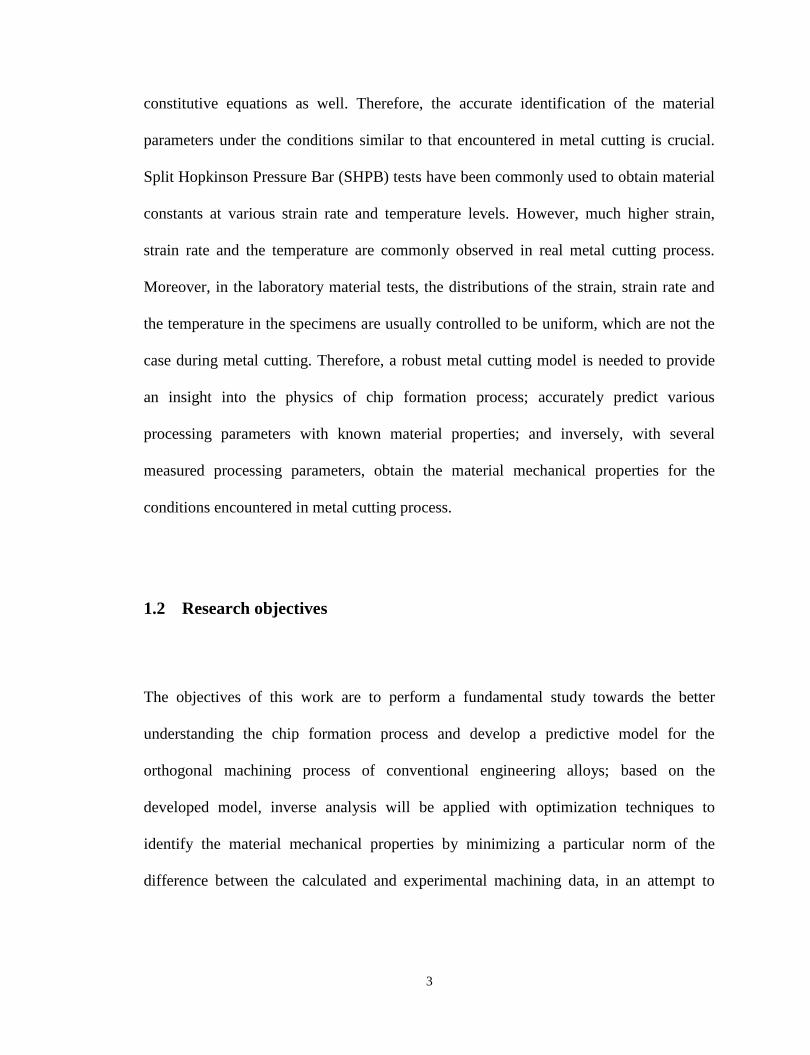
Figure 2-3 Oblique metal cutting process
In industry, most of cutting processes are performed under oblique cutting conditions.
However, the simplicity and adequacy of the orthogonal metal cutting in describing the
mechanics of machining make it favorable to researchers during the investigation of chip
formation processes. Furthermore, the orthogonal cutting is experimentally advantageous
and able to produce a reasonably good approximation of material responses to metal
cutting operation under various conditions.
2.2 Thin shear plane models
Piispanen's work, first published in 1937 and published in English in 1948 [1], applied
'pack of cards' analogy to explain the deformation pattern during chip formation process.

11
As shown in Figure 2-4, the chip formation process is represented by a deck of cards
inclined to the cutting direction with an angle . As the tool moves relative to the
workpiece, it engages one card at a time and causes it to slide over its neighbor. Each
chip segment (each card) is represented by a small thin parallelogram. Slipping occurs
between each chip segment along the shear plane.
The assumption and simplifications of the card model can be summarized as:
1) Shear action occurs on a perfectly plane surface.
2) Exaggerates the inhomogeneity of strain.
3) Does not account for the chip curl.
4) Assumes no BUE formation.
5) Interprets the tool face friction as elastic rather than plastic.
Figure 2-4 'Deck-of-Cards' chip formation model

12
In spite of the simplicity, limitations, and assumptions, this analogy of the chip formation
process presents a good illustration of how the shearing action occurs.
The first quantitative analysis of the cutting forces based on the upper bound theory was
made by Merchant[2, 3]. It was assumed that the chip of the rigid perfectly plastic
material is formed as a result of the intensive shearing along a thin shear plane, which
forms an angle with the cutting tool moving direction. The first and the most
remarkable contribution from Merchant‟s analysis is that the geometrical relationships
among the various pairs of perpendicular force components are defined in a circle with
the diameter representing the resultant force R, as shown in Figure 2-5. The force
components at the shear plane ( ), the friction force and normal force at the
chip-tool interface ( and ), the main cutting force ( ) and thrust force ( ) can be
related through the shear angle , the tool rake angle and the friction angle as shown
below
cos sins c tF F F (2.1)
sinnF R (2.2)
cos
sFR
(2.3)
sinF R (2.4)
cosN R (2.5)

13
coscF R (2.6)
sintF R (2.7)
The second contribution is that the shear angle is determined in terms of the rake
angle and the friction angle by minimizing the energy consumption during the cutting
process.
1
4 2
(2.8)
If the shear stress at the shear plane and the friction angle at the chip-tool interface
are known, with the given tool geometry and cutting conditions, the orthogonal cutting
forces can be predicted using the equations mentioned above.
The third contribution is the hodograph obtained based on the upper bound analysis. The
assumption that all the deformation takes place at a single shear plane across which the
work material turns into the chip, leads to the hodograph shown in the Figure 2-5. It can
be seen that the work material with the initial cutting velocity U suddenly changes to the
chip with the velocity . This sudden change of the velocity produces a velocity
discontinuity along the shear plane, the so-called shear velocity . With this hodograph,

14
the chip velocity and the shear velocity are able to be related to the known cutting
velocity.
sin
cosc
VV
(2.9)
cos
coss
VV
(2.10)
The force circle, the shear angle equation and the hodograph have been serving as the
foundation for the machining process research since then. The major limitations of
Merchant‟s analysis are:
1) The material is assumed to be rigid perfectly plastic, so that the effects of the
strain, strain rate and the temperature are not considered.
2) The shear strain rate along the shear plane is infinite due to the sudden change of
the velocity across the infinitely thin shear plane.
3) During the derivation of the shear angle relation, the shear angle was isolated as a
constant so that the interrelations among the shear angle and other processing
parameters were not taken into account.

15
Figure 2-5 Merchant's shear plane force circle
Lee and Shaffer [4] introduced the slip-line field analysis dealing with the plane plastic
flow problems in the plasticity theory into the area of metal cutting based on the
following assumptions:
4) The work material is rigid perfectly plastic, meaning that during the deforming
process, plastic strain overwhelmingly dominates and that the shear flow stress is
invariant throughout the deformation zone.
5) The deformation rate has no influence on the material behavior.
6) The effect of temperature increase during deformation is negligible.
7) The inertia effect as a result of material acceleration during deformation is
neglected.

16
Under these assumptions, Lee and Shaffer constructed a slip line field that consists of
two orthogonal classes of so-called slip lines, indicating the two orthogonal maximum
shear stress directions at the specific point in the plastic deformation zone, as shown in
Figure 2-6. The lower boundary of the field is formed by an idealized shear plane AC,
extending from the tool cutting edge to the point where the chip and work material free
surface intersect, and all the deformation is assumed to take place at this plane. It can be
easily realized that this shear plane is very similar to that in Merchant‟s analysis. Since
AC is the direction of the maximum shear stress, a line AB on which the shear stress is
zero is constructed along the direction 45 degree away from AC, and it serves as the
upper boundary of the field. It should be noted that in the triangular plastic zone ABC ,
no deformation occurs but the material is stressed to its yield point. Finally, assuming
that the stresses acting at the tool-chip interface are uniform, the principle stresses at AC
will meet this boundary at the angle or / 2 .The shear angle is then related to
tool rake angle and friction angle using Mohr's circle as:
4
(2.11)
Although the plastic deformation zone was realized and proposed, Lee and Shaffer did
not resolve the physics-related conflicts that result from the single shear plane model,
that is, the infinite stress and strain rate gradient across the shear plane.

17
Figure 2-6 Lee and Shaffer's slipline filed model

18
2.3 Thick deformation zone models
Okushima and Hitomi [5] assumed that rather than along a single shear plane, the
shearing should fulfill a transitional region that transforms the work material to the
steady chip. As shown in Figure 2-7, the transitional region AOB is bounded by straight
lines OA and OB, where the plastic deformation initiates and finishes respectively. OC is
the shear plane used by previous studies. Assuming the work material is rigid perfectly
plastic, the stress in the area of AOB must be in the yield state and therefore the shear
stresses on both boundaries must be equal to the yield shear flow stress,
0OA OB
(2.12)
2 2
2
cos cosOB
R
bt
(2.13)
Assuming the uniform distribution, the shear stresses on both boundaries and along the
tool-chip interface OD is obtained by means of the resultant force R on the work material
side and the chip side:
1 1
1
sin cosOA
R
bt
(2.14)
2 2
2
cos cosOB
R
bt
(2.15)

19
0
sinOD
R
bl
(2.16)
Where 1 and 2 are the inclination angles of the lower boundary and upper boundary of
the shear zone to the cutting direction. is the mean friction angle, l is the contact
length of the tool-chip interface. 1t and 2t are the uncut chip thickness and deformed
chip thickness respectively.
Equating equations (2.14~2.16), the inclination angles of lower boundary and upper
boundary can be determined.
11
2 2 2
K (2.17)
22
2 2 2
K (2.18)
1 11
2sin sin sin
tK
l
(2.19)
1 2
2
2sin sin cos
tK
l
(2.20)
From the geometry, the shear strain inside the shear zone at any given transitional line
can be expressed as follows:

20
''
'cot coti i i i
A P
AQ (2.21)
Where i is the inclination angle of the arbitrary radial plane, and i is formed by the
tangential to the point of interest on the free surface and the cutting direction. In
particular, the shear strain on the starting and ending boundary lines of flow region are
given by:
1 0 (2.22)
2 2 2cot tan (2.23)
Figure 2-7 Okushima and Hitomi's model

21
The most distinguished contribution from this work is the gradual change of the shear
strain, although in a discrete manner, can be expressed in terms of the tool rake angle and
the average friction angle. However, the effect of work hardening and the thermal
softening are still excluded.
Considering the fact that each plastic deformation is caused by shear and therefore
characterized by lines of maximum shear stress (sliplines), Zorev [6] depicted the shape
of the deformation zone with the basic knowledge of plasticity.
As shown in Figure 2-8, since LM is the free surface and sliplines stands for the planes
of maximum shear stress, each slipline should meet the free surface with an equal angle
of . To satisfy this boundary condition, these lines must be curved instead of straight.
For example, if line OL is straight, it would form an angle smaller than with the free
surface. Furthermore, there must be a deformation zone (the dotted lines) around point O
to initiate the deformation. The most part of this zone is on the chip-tool interface and
called secondary deformation zone. The shape of this zone should be influenced by the
friction boundary conditions at the chip-tool interface.

22
Figure 2-8 Zorev's schematic representation of lines of slip in chip formation
zone
All models reviewed above only reflect a particular aspect of metal cutting. The
influence of variations of cutting conditions and that of workpiece material are not
considered.
Oxley and coworkers devoted great effort into the investigation of the influence of the
material properties and the effect of strain, strain rate and temperature on the chip
formation process in a series of work [7-9], and all the achievement was crystallized in
the excellent book [10].

23
Two plastic deformation zones, namely the primary shear zone and the secondary shear
zone are considered and the shearing process are analyzed in the model, as shown in
Figure 2-9. In the primary shear zone, the so-called shear plane is opened up so that the
continuous flow of the material can be considered. Once the material particles pass
through the primary shear zone, further plastic shearing occurs in the secondary shear
zone till the end of the tool-chip contact.
Figure 2-9 Oxley's shear zone model

24
The basis of the theory is to analyze the stress distributions along the AB and tool-chip
contact interface in terms of shear angle (angle made by AB and cutting velocity) based
on the cutting conditions and work material properties. The effect of the work hardening
and thermal softening on the plastic flow behavior was taken into account. The shear
angle is selected in a manner that resultant forces transmitted by AB and the interface
are in equilibrium. Once is determined, the various components of force can be
determined from geometry relations. The most significant contribution is that Oxley and
co-workers used the velocity modified temperature concept to describe material
properties as a function of strain rate and temperature. The velocity modified temperature,
defined as mod
0
1 lg ABT T
increases as the temperature increases and decreases
as the strain rate increases. The parameters and 0 are the constants for a given
material. The flow stress is related to the strain through the power law
mod
1 mod
n TT , where both strength coefficient 1 and the strain hardening
exponent n , are functions of velocity modified temperature. The detailed demonstration
of the methodology will be introduced in the later sessions.
The following is the list of assumptions and limitations in the Oxley's model:
1) The shear strain rate is constant through the shear zone.
2) The shear stress is constant along shear plane AB.

25
3) Half of the overall shear strain occurs at AB.
4) The effect of temperature gradient is neglected.
5) The effect of strain rate gradient is neglected.
6) The distribution of the hydrostatic pressure alone AB is linear with A BP P .
7) The distribution of normal stress at chip-tool rake interface is uniform.
8) The shear stress along chip-tool rake interface is constant.
9) Sticking dominates in secondary shear zone and the shear strength in the chip
material adjacent to the tool-chip interface will be used to represent the friction
parameter.
10) The hodograph is adopted from that for single shear plane model so that velocity
discontinuity still exists.
Although sweeping assumptions and simplifications were utilized, Oxley's machining
theory still serve as a great breakthrough toward the understanding of the machining
process.
2.4 Oxley's predictive machining theory
Based on experimental observations of the material deformation, Oxley and coworkers,
under the assumptions of plain strain and steady state conditions, developed a class of
theoretical relationships between orthogonal machining process variables and workpiece

26
material properties, tool geometry and cutting conditions. The essential machining
characteristics, such as temperature in metal cutting deformation zones, deformed chip
geometries, cutting forces etc, can be obtained mathematically, meaning no need for pre-
experiments to calibrate several specific cutting constants, which are essential in
traditional machining models.
To account for the effect of work hardening of the material, the shear plane AB need to
open up to form a deformation zone, so that there is space and time for the material to be
deformed and hardened. As shown in the simplified Oxley‟s parallel-sided chip
formation model (Figure 2-10), the primary shear zone is assumed to be parallel-sided
and the secondary shear zone is simplified as a rectangle with constant thickness. The
geometry of the primary deformation zone is defined through the parameter 0C , which
represents the ratio of the length of primary deformation zone ( ) to its thickness. The
parameter is used to represent the relative thickness of the secondary deformation
zone with respect to the deformed chip thickness.

27
Figure 2-10 Simplified representation of parallel-sided deformation zones
Utilizing the same velocity diagram as in the single shear plane model, the chip velocity
V , the shear velocity SV and normal velocity on the main shear plane NV can be related
to the cutting velocity U ,
sin
cos
UV
(2.24)
cos
cosS
UV
(2.25)

28
sinNV U (2.26)
Assuming the distance from CD to AB is equal to that from AB to EF and the strain
distribution is linear, the shear strain at AB is then taken as half of the total strain
1 1 cos
2 2 sin cos
SAB
N
V
V
(2.27)
By assuming a maximum value at AB, the average value of shear strain rate along AB is
developed in terms of the shear velocity and the thickness of the primary shear zone.
0S
AB
AB
VC
l (2.28)
in which the length of the main shear plane AB, in terms of feed rate is determined by
geometric relation.
1
sinAB
tl
(2.29)
The shear strain and strain rate in the secondary shear zone, considering its rectangular
shape, are expressed as follows.
int
2
H
t
(2.30)

29
int
2
V
t
(2.31)
in which H is the chip tool contact length, is the chip thickness, so that is the
thickness of the secondary shear zone.
Applying Boothroyd temperature model [11], the temperature at AB is given by the
following equation.
AB w szT T T (2.32)
1
cos1
cos
Ssz
FT
St w
(2.33)
The specific heat S and thermal conductivity K are expressed as fitted empirical
equations in terms of the temperature and the percentage of chemical components in the
carbon steels.
420 0.504 ABS T (2.34)
4
0418.68 0.065 0.065 1.0033 11.095 10 ABK K T (2.35)
0 1/ (5.8 1.6[ ] 4.1[ ] 1.4[ ] 5[ ] [ ] 0.6[ ] 0.6[ ])i n r oK C S M P Ni C M (2.36)

30
is the proportion of heat conducted into the workpiece which can be determined,
through a non-dimensional thermal number TR ,with empirical equations (2.37~2.39)
obtained by curve fitting to Boothroyd‟s experimental results.
0.5 0.35lg tan for 0.04 tan 10.0T TR R (2.37)
0.3 0.15lg tan for tan 10.0T TR R (2.38)
1T
SUtR
K
(2.39)
With the obtained temperature and shear strain rate, the velocity modified temperature
, a variable that combines the effects of temperature and strain rate, is applied to
describe material flow behavior by Equations (2.40) and (2.41),
mod
1 mod
n T
AB T (2.40)
mod
0
1 lg ABABT T
(2.41)
in which the equivalent flow stress, strain and strain rate are related to the shear stress,
strain and strain rate according to the Von Mises flow rule using Equations (2.42~2.44).
3AB ABk (2.42)

31
3
ABAB
(2.43)
3
ABAB
(2.44)
Once ABk is determined, the shear force at AB can be obtained from the geometric
relations given in the Merchant's circle (see Figure 2-5).
1
sin
ABS
k t wF
(2.45)
By noting that both material thermal properties and shear force are interrelated with
temperature, the temperature along AB should be calculated iteratively until it reaches
steady state.
Applying the appropriate stress equilibrium equation along shear plane AB, the angle
between resultant force and shear force is given as follows.
0
1tan 1 2
4C n
(2.46)
The mean friction angle can be found geometrically by the relation
(2.47)
32
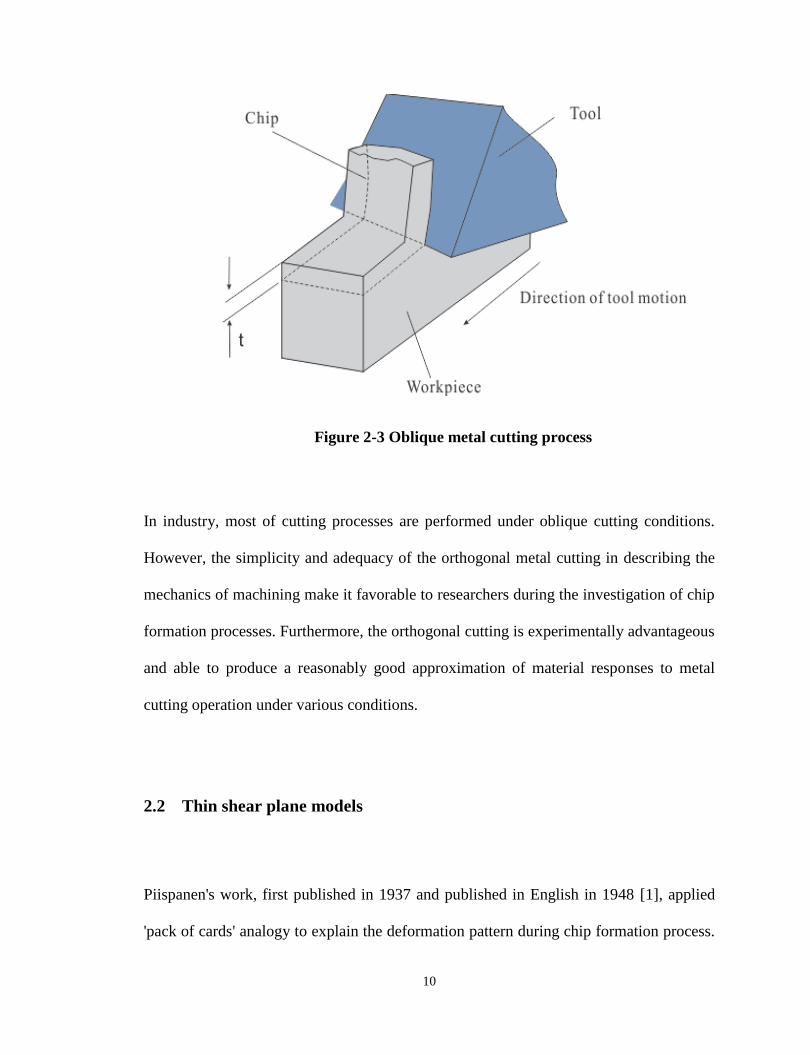
After all the calculations above, the deformed chip thickness and desired force
components can be determined with a given shear angle.
1
2
cos
sin
tt
(2.48)
cos
SFR
(2.49)
cos( )CF R (2.50)
sin( )TF R (2.51)
sinF R (2.52)
cosN R (2.53)
Assuming uniform distribution of the normal stress along the tool-chip interface, the tool
chip contact length is obtained by satisfying the condition that the moment of the normal
force about point B equals the moment of the resultant force along AB.
01
0
sin1
cos sin3 1 2
4
C ntH
C n
(2.54)
The average temperature at the tool-chip interface is defined as
int w sz MT T T T (2.55)

33
1
22 20.06 0.195 0.5lg
10
T TR t R t
h h
M CT T
(2.56)
1
sin
cosC
FT
St w
(2.57)
Iteration is needed as well until the steady state is reached.
The maximum shear strain rate, which is assumed to occur at the tool-chip interface for
the secondary shear zone, can be found from Equation (2.58).
int
2
V
t
(2.58)
Realizing the fact that the flow stress will be overestimated if Equation (2.40) is applied
to the secondary shear zone, Oxley used this equation with strain always equal to one to
neglect the influence of strain greater than 1 on flow stress. Therefore, the chip flow
stress expression for secondary deformation zone is modified as
1
3chipK
(2.59)
The shear stress at tool-chip interface can also be expressed in terms of the resultant
force obtained from the stress analysis on AB, that is
int
F
hw (2.60)

34
Trying out a range of values, the final shear angle is selected as the one that meets the
condition that resolved shear stress at the tool-chip interface expressed in Equation (2.59)
and the shear flow stress formulated by Equation (2.60) are in equilibrium.
For the uniform normal stress distribution as assumed, the average normal stress at the
tool-chip interface is given by
NN
hw (2.61)
In order to determine , the normal stress on the tool-chip interface is also found from
the stress boundary condition at B by working from A along AB, and it can be expressed
as
0
11 2 2
2N
AB
C nK
(2.62)
The final value of can now be fixed at the one that makes the normal stress at tool-
chip interface calculated both way equal to each other.
Finally, the constant is determined by considering the minimum work principles. That
is, the whole analysis is repeated for a set of different values and the final is taken as
the one minimizing the cutting force.

35
CHAPTER 3.
EXTENSION OF OXLEY'S MACHINING THEORY
FOR VARIOUS MATERIALSEquation Chapter (Next) Section 1
3.1 Introduction
The predictive machining theory developed by Oxley and coworkers, in which the
machining characteristic factors are predicted from input data of workpiece material
properties, tool geometry and cutting conditions, is an enlightening example of how to
analyze the metal cutting and provides us the possibility of expressing the machining
process physically and mathematically. However, there is still some challenging work to
prepare for the prediction. It is essential to conduct high speed compression tests for
preparing proper material property data such as flow stress versus velocity modified
temperature and strain-hardening index versus velocity modified temperature. A curve
fitting method is also needed to express the flow stress and strain-hardening index in the
universal formulae for different kinds of cutting conditions of the experimental

36
workpiece material. This fact makes the availability of whole class of solutions restricted
to a relatively narrow range of materials. . In order to apply Oxley‟s machining theory to
a wider range of materials, Johnson-Cook constitutive material model [12], in which the
constants are available for most commonly machined materials, is adopted in this work
to represent the material flow stress or flow behavior under cutting conditions.
3.2 Description of Johnson-Cook material model
The general structure of Johnson-Cook material model is given in equation
0
0 0
1 ln 1
m
n
m
T TA B C
T T
(3.1)
In the above equation, is the equivalent flow stress, is the plastic equivalent strain,
and 0 are equivalent strain rate and reference strain rate respectively, and T ,mT ,
0T
represent instantaneous temperature of the material, melting temperature of the material
and the ambient temperature, respectively. The five material constants A, B, C, m, n are
the constants that need to be determined from experiments. The physical significance of
the five parameters are
1) A represents the initial yield strength
2) B and n account for the strain hardening effect.
3) C accounts for the deformation rate sensitivity.

37
4) m considers the thermal softening effect.
3.3 Generic constitutive equation based analysis
Based on the Johnson-Cook model and Von Mises‟ flow rule, the material shear flow
stress at AB can be expressed as:
0
11 ln 1
3
m
n AB wABAB AB
m w
T Tk A B C
T T
(3.2)
The equilibrium equations of the slipline field are in the form
1 1 2
2 0 along linep k
kS S S
(3.3)
2 2 1
2 0 along linep k
kS S S
(3.4)
Assuming the material is perfectly plastic, the solution of Equations (3.3) and (3.4) leads
to the well known Hencky's equations.
2 along linep k const (3.5)

38
2 along linep k const (3.6)
When strain hardening effect is considered, Equation (3.3) and (3.4) can be solved as
1
2
2 along linek
p k dS ConstS
(3.7)
2
1
2 along linek
p k dS ConstS
(3.8)
As discussed in section 2.42, the main shear plane as a slipline must be curved in order
to satisfy the boundary conditions. Oxley [10] assumed the sliplines are in the shape as
shown in Figure 3-1. The shear plane A'B' is considered as a line and the chip-tool
interface is taken as a line. The line is assumed to be straight for the most part (AB),
in order to simplify the calculation. The line turns from point A to A' to meet free
surface with an angle in order to satisfy the free surface boundary condition. On the
other, the line turns from B to orthogonally meet the tool rake face at B'. However, the
length of AA' and BB' are assumed to be short enough for the effect of strain hardening
from A to A' and B to B' to be ignored. Another word, the straight line AB can represent
the main shear plane.

39
Figure 3-1 The assumed curve of the main shear plane as a slipline
According to Hencky's equation,
' '2 2A AB A A AB AP k P k (3.9)
in which
'4
A
A
(3.10)
Since A' is the intersection of slipline and free surface,

40
'A ABP k (3.11)
Substituting Equation (3.10) and (3.11) into (3.9), the hydrostatic stress at point A is
obtained.
1 24
A ABP k
(3.12)
Similarly, AB turns an angle of ( to the point B'. therefore, the normal stress on
the chip-tool interface can be expressed as
' 2N B B ABP P k (3.13)
Applying Equation (3.3) and noting that the slipline AB is straight, i.e.
, one can
obtain
1
0 2
ABB
A
lP
P
dkdP dS
dS
(3.14)
Further assuming does not change along , Equation (3.14) becomes
2
A B AB
dkP P l
dS (3.15)
in which the shear flow stress is a function of shear strain , shear strain rate and
temperature , so that
2 2 2 2
dk k k k T
dS S S T S
(3.16)

41
The second and the third terms in Equation (3.16) can be taken as zero since 1) at main
shear plane AB, the strain rate reaches the maximum and 2) the gradient of temperature
is negligible at the steady state. Thus, the following relation exists.
2 2 AB
dk dk d dt
dS d dt dS
(3.17)
where k is shear stress, is shear strain, 2s is the thickness of primary shear zone
and t is time.
For the Von Mises material, the first term on the right hand side of Equation (3.17) can
be written as
/ 3 1
33
AB AB AB
AB ABAB
dk d d
d dd
(3.18)
Using Johnson-Cook model, following equation can be obtained:
1
0
1 ln 1
m
n AB wAB ABAB
AB m w
T TdnB C
d T T
(3.19)
By noting that AB
d
dt
is the shear strain rate along AB and
2 AB
dt
ds is the reciprocal of the
velocity normal to AB, as shown in Equation (3.20) and (3.21) respectively.
0 0
cos
cos
S
AB AB AB
Vd UC C
dt l l
(3.20)

42
2
1
sinAB
dt
ds U (3.21)
The change rate of flow stress normal to AB 2
dk
ds can finally be expressed with Equation
(3.22) :
0
2
2n
ABAB
n
AB AB
C nBkdk
ds l A B
(3.22)
Since the slip lines are assumed to be straight, the equilibrium of the slip line field gives
0
2
2n
ABA B AB AB n
AB
C nBdkP P l k
ds A B
(3.23)
Substituting Equation (3.12) into (3.23), the hydrostatic stress at point B can be obtained.
021 2
4
n
ABB AB n
AB
C nBP k
A B
(3.24)
Once the hydrostatic stresses AP and BP are determined, with the assumption of linear
distribution of normal pressure on the shear plane AB, the normal force acting on AB NF ,
the shear force along AB SF , and the angle made by resultant force and the line AB
can be obtained.
2
A BN AB
P PF l w
(3.25)
S AB ABF k l w (3.26)

43
0tan 1 24
n
N AB
n
S AB
F C nB
F A B
(3.27)
Taking the chip as a free body bounded with the main shear plane AB and the chip-tool
interface, and assuming that the resultant force R acting on the shear plane AB is
collinear with the resultant force R' on the chip-tool interface, the forces exerting on the
chip are shown in Figure 3-2. and are the location of R and R' measured from
cutting edge (point B). Angle and are the angles made by R with the shear plane and
by R' with the normal force on the chip-tool interface respectively.
Taking the moment of the resultant force R about the tool tip B, one can see
02
ABl
A BA BAB sh B
AB
P PP Pwl X P x xdx
l
(3.28)
Solving Equation (3.28) leads to
2
3
A Bsh AB
A B
P PX l
P P
(3.29)
From sin law, can be expressed in term of
int
sin
cosshX X
(3.30)

44
Assuming uniform distribution of the normal stress on the tool rake face, the chip tool
contact length H is
int2H X (3.31)
Substituting Equation(3.12), (3.24), (3.29) and (3.30) into Equation (3.31), the chip-tool
contact length H can be obtained.
01 1
0
sin 2 sin21
3 cos sin cos sin3 1 2
4
n
ABA B
nA BAB
C nBt P P tH
P PC nB
(3.32)
The flow chart is given in Figure 3-3.
3.4 Conclusion
In this chapter, Oxley's parallel-sided thick zone model is extended by substituting
Johnson-Cook‟s constitutive material model for the counterpart used by Oxley and
Coworkers. This approach generalized the applicability of the model to a wide range of
materials commonly used in industry. The result developed in this chapter is the very
basis for the further extension and modification of the theory in later chapters. Therefore,
the preliminary verification is omitted for this chapter. The experimental verification of
the models in Chapter 4~Chapter 7 will be presented correspondingly.

45
Figure 3-2 Forces acting on the chip as a free body

46
Figure 3-3 Flow chart of the methodology for the simulation of orthogonal
cutting process

47
CHAPTER 4.
END MILLING SIMULATION Equation Chapter (Next) Section 1
4.1 Introduction
Milling operations are one of the most common machining operations in industry.
Milling, as a versatile material removal process, can be used for face finishing, edge
finishing, material removal, etc. Most complicated shapes can be machined with close
tolerances by using milling operations.
Most of the current models for analysis of 3D milling processes are empirically based
semi-analytical models with the primary aim of predicting cutting forces without getting
involved in the physics of the process and root cause of different phenomena occurring
in machining. These models require experimentation to find a few calibration constants
that establish a close relationship between the model predictions and measured values for
different cutting parameters. These techniques (mechanistic methods) are reliable,

48
however, the coefficients that govern the force models are often restricted to a particular
operation and the condition tested.
In this chapter, an analytical force model for the helical end milling tool is developed by
extending the orthogonal chip formation model developed in Chapter 3 to that for
oblique cutting conditions.
4.2 Mechanics of milling process
Milling is a process of removing material from the workpiece by feeding the work piece
past a rotating multipoint cutter. Since the milling cutter is held in a rotating spindle with
a fixed axis while the workpiece clamped on the table is moving linearly toward the
cutter, the path of each of the milling cutter teeth forms an arc of trochoidal. As a result,
varying but periodic chip thickness is generated at each tooth-passing interval.
In practice, there are three types of milling operations commonly used in industry:
1. Up milling operation, also referred to as conventional milling, is characterized by
the opposite direction of cutter rotation to the workpiece feed direction. In up
milling, the formation of chip begins with a small load as the flute begins to cut
and then increases gradually to the maximum right at the location where the flute
exits the cutting region. See Figure 4-1.

49
Figure 4-1 Up milling
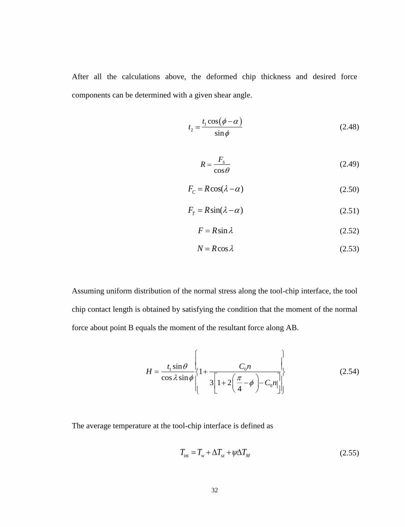
2. Down milling operation, also known as climb milling, works in an inverse
manner to up milling. That is, the cutter rotates in the same direction as the
motion of the feed and the chip load decreases from a maximum value to zero
during the cutter flute passing through the cutting region. See Figure 4-2.
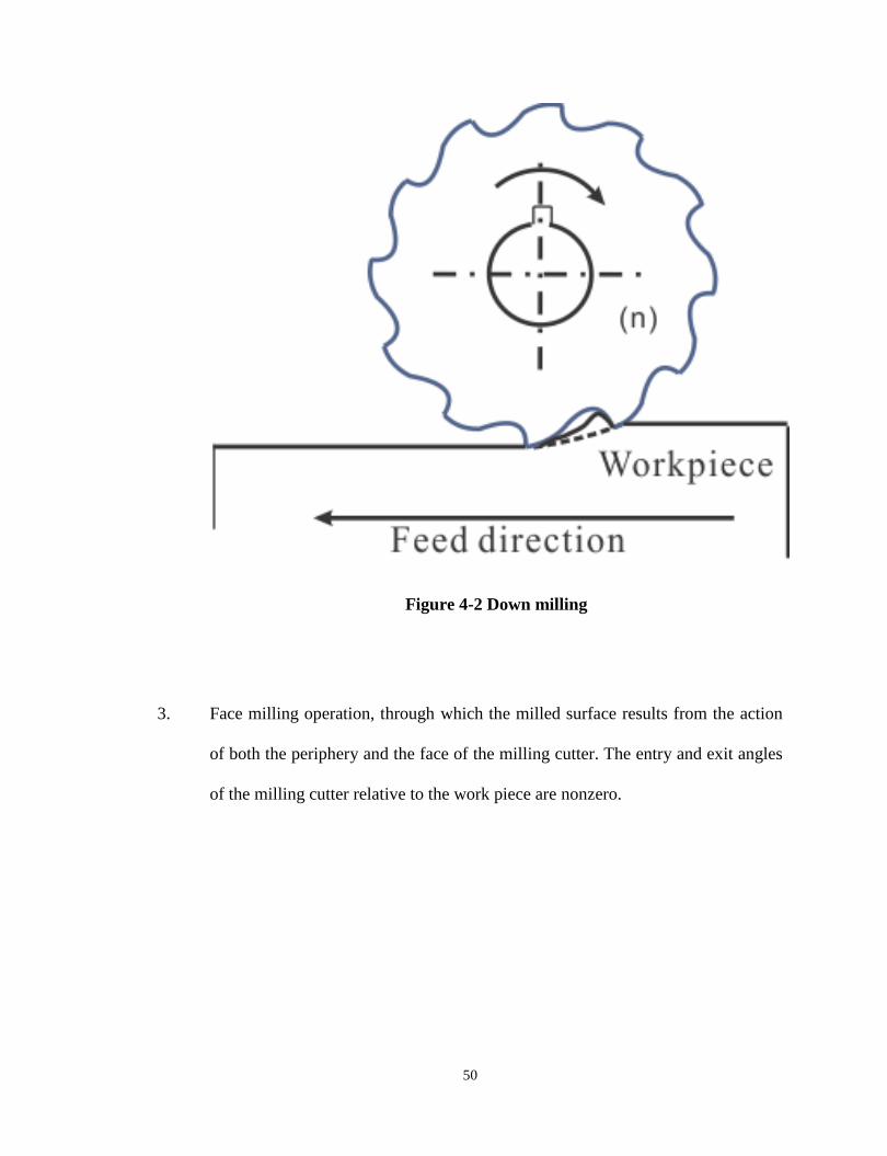
50
Figure 4-2 Down milling
3. Face milling operation, through which the milled surface results from the action
of both the periphery and the face of the milling cutter. The entry and exit angles
of the milling cutter relative to the work piece are nonzero.

51
Figure 4-3 Face milling
The complexity of the milling tooth track makes the milling process inimical to
mathematical treatments. On the other hand, the great similarities existing between
milling and conventional oblique cutting operations could facilitate the analysis by
treating the operation of every single flute as that of a single point cutting tool with
relatively complicated geometry and kinematics.
52
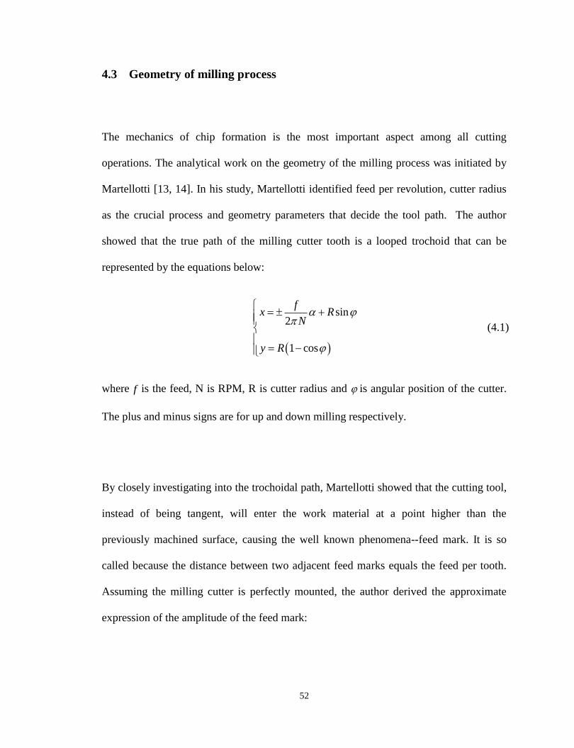
4.3 Geometry of milling process
The mechanics of chip formation is the most important aspect among all cutting
operations. The analytical work on the geometry of the milling process was initiated by
Martellotti [13, 14]. In his study, Martellotti identified feed per revolution, cutter radius
as the crucial process and geometry parameters that decide the tool path. The author
showed that the true path of the milling cutter tooth is a looped trochoid that can be
represented by the equations below:
sin2
1 cos
fx R
N
y R
(4.1)
where f is the feed, N is RPM, R is cutter radius and is angular position of the cutter.
The plus and minus signs are for up and down milling respectively.
By closely investigating into the trochoidal path, Martellotti showed that the cutting tool,
instead of being tangent, will enter the work material at a point higher than the
previously machined surface, causing the well known phenomena--feed mark. It is so
called because the distance between two adjacent feed marks equals the feed per tooth.
Assuming the milling cutter is perfectly mounted, the author derived the approximate
expression of the amplitude of the feed mark:

53
2
8
tfhR
(4.2)
Under the condition of tool eccentricity, a wavy machined surface will be generated with
a frequency equal to that of the cutter rotation. He also illustrated that the severity of the
feed mark could be diminished by decreasing feed per tooth and increasing cutter radius.
Martellotti has also shown that the tooth path is almost circular for light feeds. In most
real cutting condition, it is always true that feeds are much smaller than cutter radius.
Therefore, the tooth path is simplified to a circle by Martellotti and the chip thickness
equation was derived:
sinct f (4.3)
Because of its reasonable accuracy, this equation has been used in almost all milling
studies. Other than this, the average chip thickness, obtained by integrating Equation
(4.2) over the rotational range from entry to exit angles and divided by the range of the
cut, is derived as following:
en
ex
c c
en
f Rdt t d
R
(4.4)
4.4 Mechanistic models for milling process

54
Milling force models generally fall into five categories according to increasing levels of
sophistication and accuracy, as classified by Smith and Tlusty [15]:
Average rigid force, static deflection model
Instantaneous rigid force model
Instantaneous rigid force, static deflection model
Instantaneous force with static deflection feedback
Regenerative force, dynamic deflection model
The simplest milling force model is the “average rigid force model” which assumes that
the average power consumed in the cutting is proportional to the material removal rate.
The average cutting forces calculated this way are then applied to calculate static
deflections of the tool treated as a cantilever beam. The work of Wang [16] is a standard
example of this kind of model. Although the “average rigid force model” is a very good
“first approximation”, as mentioned by Smith and Tlusty [15], it considers neither force
variations inherent in intermittent cutting nor the influence of the tool deflection on the
cutting forces. For more accurate predictions, the cutting forces at the tooth tip should be
considered.
The “instantaneous rigid force model” calculates the milling forces based on the
instantaneous chip load. This way, the weakness cited from the “average rigid model” is
basically overwhelmed. However, the deflection of the cutter is not considered in the
force calculation. The “instantaneous rigid force, static deflection model” is developed

55
essentially based on the “instantaneous rigid model” and includes the static deflection
calculation. It‟s called “static deflection” for the reason that the cutter deflection is
considered as proportional to the cutting forces, without taking system inertia into
consideration. The “instantaneous force with static deflection feedback model” is further
improved from previous models by an iterative deflection calculation, in which the force
and deflection are correlated. Finally, the “regenerative force, dynamic deflection model”
combines all the advantages of previous models and further accounts for system inertia.
The chatter and forced vibration phenomena associated with milling operations can also
be accurately depicted by this model.
In general, except the “average rigid force, static deflection model”, the other four kinds
of models are based on the same root—the instantaneous force. Because it is more
realistic, most researches on the milling process have been following this idea.
The pioneer work, based on Martellotti‟s analysis of the kinematics of the milling
process, was started by Konnisberger and Sabberval [17, 18]. They studied tangential
forces in detail and showed that two components of the cutting force vector could be
predicted by using tangential and radial force components at any location on the cutting
edge. The local tangential force is related to the instantaneous chip section and the local
radial force is proportional to the tangential force:
x
t t cF K bt (4.5)

56
r r tF K F (4.6)
where tF is tangential force, rF is radial force, b is the width of cut, ct is the
instantaneous chip thickness calculated by Equation (4.3), tK , rF are defined as specific
cutting forces, representing the cutting forces per unit area and vary with width of cut,
depth of cut and feed. x is a process constant having common values of 0.7 to 0.8.
The same method was utilized by Kline [19, 20] to study problems of cornering and
forging cuts. He considered the milling cutter consisting of a series of orthogonal cutter
disk segments. Each segment is rotating with respect to adjacent segment having
different chip thickness. The total force acting on the cutter at a given angular position
can be obtained by analysing local cutting model and summing up the forces acting on
the individual cutter segments. Other than this, Kline considered the effect of cutter
runout and incorporated it into the calculation of chip load. Furthermore, by assuming
the cutter to be a cantilever beam, the tool deflection was calculated from the cutting
forces predicted from the proposed model and was used to analyze the machined surface
error. So far, the “milling force model” has developed to the third level, “Instantaneous
rigid force, static deflection model”.
Sutherland and Devor [21] improved Kline‟s method to predict cutting forces in flexible
end milling systems. In this model, the effect of system deflections on the chip load was
taken into account and the instantaneous chip thickness was solved based on the balance

57
between cutting forces and resulted cutter deflections. Later, based on the pioneer
investigation on the end milling dynamics by Tlusty [22], Sutherland [23] further
sublimated the model to the vertex, the “Regenerative force, dynamic deflection model”.
Armarego and Deshpande [24] further studied and discussed the importance of both
cutter runout and deflection on the cutting force fluctuations. In this study, three models,
namely the „ideal‟ model for rigid cutter with no eccentricity, the rigid cutter
„eccentricity‟ model and the more comprehensive „deflection‟ model, were assessed by
experimental data. It‟s shown in this study that:
All three models provide good predictions of average cutting forces and torques.
Both the „eccentricity‟ and „deflection‟ models yield satisfactory results for force
fluctuation predictions.
The „deflection‟ model gives the best result in all cases, especially for the heavy
cutting conditions under which undesirable cutter deflections commonly happen.
However, the efficacy of this comprehensive model is traded off by the excessive
computer processing time.
Yucesan et. al [25-27] considered rake angle and evaluated the varying friction and
pressure acting on the tool-chip interface. They developed a 3D cutting force prediction
system for helix end milling process, in which cutting force coefficients ( nK , fK ) and
chip flow angle ( c ) are considered to vary with cutter rotation angle:

58
n n cdF K dA (4.7)
f f n cdF K K dA (4.8)
where nK and fK are specific cutting coefficients. The values of these specific energies
depend on the tool and workpiece materials as well as tool geometry and cutting
conditions. Yucesan and coworkers observed the high dependence of nK and fK on the
chip thickness ( ct ), cutting speed ( V ) and normal rake angle ( n ), the empirical
equations relating the specific energies to them were developed:
0 1 2 3 4ln ln ln ln ln lnn c n cK a a t a V a a t V (4.9)
0 1 2 3 4ln ln ln ln ln lnf c n cK b b t b V b b t V (4.10)
where 0 4a a and 0 4b b are experimentally determined. Once the normal and friction
forces are determined, they can be transformed into global coordinate system.
Wang and Liang [28, 29] analysed the flat-end milling forces via angular convolution
and established a close form angular convolution model for the prediction of cutting
forces in the cylindrical end milling processes.
Following these works, a numerous of mechanistic models have been developed based
on either one or more works described above. All of these models are assuming that the

59
cutting forces can be related to the chip load through cutting specific energies which
have to be determined from calibration experiments.
4.5 Analytical modeling of milling forces
In the current study, the milling force simulation is based on the orthogonal force model
developed in Chapter 3, so that experimental calibrations can be avoided. Geometric
considerations must be made to use the analytical orthogonal model described in the
previous chapter. As shown in Figure 4-4, the cutting flutes are modeled as discrete
linear segments. Every flute on each segment can be treated as a single point cutting tool
executing oblique cutting. Orthogonal cutting force model can be applied after the
oblique-to-orthogonal conversion. The total force acting on the milling cutter can be
found by summing up the forces acting on every flute segment of a given disk for a
given tool angular position.

60
Figure 4-4 Segmented milling tool model
4.5.1. Angular position
In order to model the milling process, the position of every cutting point in the fixed tool
coordinate system needs to be known. Referring to Figure 4-5, if i, j and k are defined as
the flute number, the rotational increment number and the segment number respectively,
every flute segment has a particular angular position for a set i-j-k combinations.
The angular position of the cutter is denoted by:

61
( )j j (4.11)
where is the angular increment as the tool rotates.
At the moment when the cutter starts to rotates, if the bottom of any of the flute is
located at the position with zero rotation angle, the angular position of the bottom on any
other flute can be defined as
2
p
d
in
(4.12)
where dn is the total number of flutes on the cutter. The term 2
dn
is the so-called pitch
angle, the angular spacing between cutting flutes on an evenly fluted milling cutter.
Because of the helix angle, angular positions of each point along a specific cutting flute
in the tool coordinate system are different. This angular difference is defined as lag angle
l . For a specific flute, the angular position at the k_th axial segment with respect to the
bottom can be expressed in terms of the helix angle hx ,
tan( )l hx
a
ak
R
(4.13)
In which a is cutting width of the elemental flutes (the axial depth of a disk element),
aR is the radius of the milling cutter.

62
Combining these elements, a generalized expression of the angular position for an
arbitrary cutting point in the tool coordinate system can be derived as
2
( , , ) tan( )hx
d a
ai j k j i k
n R
(4.14)
Figure 4-5 Geometry of cutting tool

63
4.5.2. Chip load calculation
Uncut chip thickness in milling operation can be defined as the portion left between two
consecutive flute segments on the same disk. It‟s contributed by feed-per-tooth, but
changes as the tool rotates. By assuming the tooth path to be circle, as suggested by
Martellotti [13], the instantaneous uncut chip thickness , as shown geometrically in
Figure 4-6, is calculated as following.
( , , ) sin , ,u xt i j k f i j k (4.15)
This formula applies only to the condition under which the rotation axis of the spindle
coincides with the geometrical axis of the milling cutter. In this case, each tooth has
exactly the same radius and removes the same amount of material.

64
Figure 4-6 Chipload in end milling
Cutter runout, referring to the state of tool cutting points rotating about an axis different
from the geometrical axis, is a commonly existing phenomenon in machining. It can
either be in the form of an offset, a tilt, or a combination of both.
The type of runout involving a cutter axis offset is termed radial runout, while the type
involving a cutter axis tilt is referred to as axial runout [30]. The magnitude of axial
runout is usually small relative to the axial depth of cut, plus considering the difficulty of
measurement, only radial offset will be considered in this study.

65
Figure 4-7 shows an end mill radial offset in a tool holder, where the runout angle run
is defined to be the angle between the negative Y axis direction and the line connecting
the spindle rotation center and the tool geometry center. is runout amplitude. When
radial offset exists, each flute at every point along the axis of the cutter experiences a
different chip thickness than predicted by Martellotti‟s approximate equation. The chip
thickness generated by a specific cutting point depends on the effective radius of the
flute and the effective radius of the other flutes as well. From the geometry in Figure 4-7,
the following expression can be derived as the radial length from center of rotation to the
cutting edge at given index numbers i and k.
2 2( , ) 2 cos( ( , 0, ))e a run a run runR k i R R i j k (4.16)
(a) Schematic demonstration of radial runout

66
(b) Runout, cutter radius and effective cutter radius
Figure 4-7 Radial offset runout of the milling cutter
Once the effective radius is known, the chip thickness h at a specific angular position, as
illustrated in Figure 4-8, is
( , , ) ( , )eh i j k R k i d (4.17)
where
2 2 2( , 1) cos ( ( , , )) sin( ( , , ))e x xd R k i f i j k f i j k (4.18)

67
Figure 4-8 Chip thickness diagram during end milling[19]
To account for the situation when runout is very serious, Equation (4.17) can be
modified as
( , , ) ( , ) ( , ( , , )) ( , , ) sin( ( , , ))e e xh i j k R k i R k i m i j k m i j k f i j k (4.19)
( , , )m i j k is an integer, counting from 1 to the value of the total flute number. For
example, if the cutter contains 4 flutes, ( , , )m i j k will count from 1 to 4. Every time if the
previous cutting flute has removed the material, the value of ( , , )m i j k is set to 1 when
calculating the uncut chip thickness for the current cutting flute at the same height. If the
previous cutting flute failed to cut, the value of ( , , )m i j k is increased by 1. In simulation,

68
for example, if the first flute cut, the second and the third flute have all failed to cut, the
value of ( , , )m i j k is set to 3.
4.5.3. Entry and Exit angle
Because milling is an intermittent cutting process, an additional factor should be
considered when modeling the milling process: whether or not the flute is engaged into
cutting. The angular region in which the cutter is engaged in cutting is known as the
immersion angle. The angles at which the flute begins to cut and exit to cut are called
entry angle and exit angle, respectively. An illustration of the immersion angle for two
main types of milling is shown in Figure 4-9.

69
Figure 4-9 Demonstration of immersion angles

70
For up milling with a cutter radius aR and radial depth of cut ad , the entry angle en is
zero and the exit angle ex is given by
1cos 1 aex
a
d
R
(4.20)
When the cutter offset exists, the approximation of zero entry angle may not be able to
reflect the cutting geometry accurately. From the geometry of Figure 4-10, the general
expression of the entry angle en can be derived by using the cosine law:
2 2 2
1 ( , , ) ( , ) ( , ( , , ))( , , ) cos
2 ( , , ) ( , ) 2
x a aen
a x
m i j k f R k i R k i m i j ki j k
m i j k R k i f
(4.21)
It can be seen that when runout doesn‟t exist, Equation (4.21) becomes
1cos2 2
xen
a
f
R
(4.22)
when a xR f , 0en .
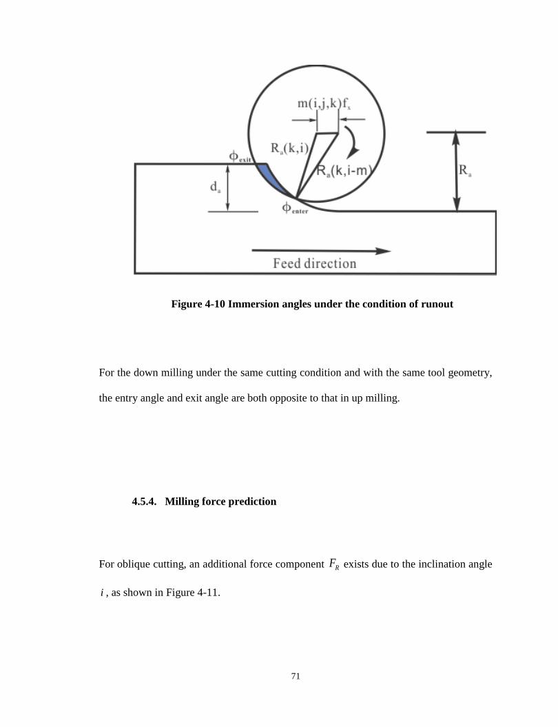
71
Figure 4-10 Immersion angles under the condition of runout
For the down milling under the same cutting condition and with the same tool geometry,
the entry angle and exit angle are both opposite to that in up milling.
4.5.4. Milling force prediction
For oblique cutting, an additional force component RF exists due to the inclination angle
i , as shown in Figure 4-11.

72
Figure 4-11 Conventional Oblique Cutting Forces
As stated in [10], for a given normal rake angle n and other cutting conditions, the
forces CF and tF are almost independent of inclination angle i , and the chip flow angle
c approximately satisfies Stabler‟ flow rule [31], which can be expressed as:
c i (4.23)
It means that the cutting force CF and the thrust force tF in oblique cutting can be
determined from the orthogonal theory by taking inclination angle as zero. By noting this

73
and realizing that the resultant force R must be acting in the plane containing tool-chip
friction force and normal to the tool rake face, Hu et.al [32] developed an expression for
rF in the following way:
With regard to Figure 4-11, the resultant force R can be expressed in vector form
ˆˆ ˆC t rR F c Ft F r (4.24)
c , t , r are unit vectors in cutting force, thrust force and radial force directions,
respectively.
The three unit vectors along the main cutting edge, normal to main cutting edge and the
chip flow direction can, from geometry, be expressed in terms of the normal rake angle
n and the chip flow angle c , as shown in the following equations.
ˆ ˆ ˆsin cosa ic ir (4.25)
ˆ ˆˆ ˆsin cos cos sin sinn n nb ic t ir (4.26)
ˆˆ ˆsin cosc cq a b (4.27)
The unit vector normal to the rake face plane (i.e. the plane made by a and b ) is found by
the cross product of a and b :

74
ˆ ˆˆ ˆ ˆ ˆcos cos sin cos sinn n nn b a ic t ir (4.28)
The unit vector normal to the plane where the resultant force R lies in (i.e. the plane
made by n and q ) can be expressed in the same way:
ˆ ˆ ˆ
ˆˆ (sin cos sin cos sin ) cos sin
ˆ (cos cos sin sin sin )
c n c n c
c n c
p q n
i i c t
i i r
(4.29)
Noting that R and p are normal to each other, their inner product should be zero:
ˆ 0p R (4.30)
Finally, the radial force rF is derived:
sin cos sin tan cos tan
sin sin tan cos
C n c t n c
r
n c
F i i FF
i i
(4.31)
Once rF was obtained, based on the geometrical analysis on tube end cutting with side
cutting angle sC (Figure 4-12) the cutting force components in the machine tool
coordinate system was achieved:
1 CP F (4.32)
2 cos sint s r sP F C F C (4.33)
3 sin cost s r sP F C F C (4.34)

75
Where the positive directions of 1P , 2P and 3P are taken as the cutting velocity, negative
feed and outward radial directions.
Figure 4-12 Tube-end oblique cutting forces
Utilizing the geometrical similarities between end tube turning and face milling, Young
et.al [33] developed a face milling force model for single edge fly cut. The whole cutting
process was modeled as an end tube turning process with a variable chip thickness.
For the peripheral part of the end miller, the side angle sC is 0. Equation (4.32~4.34)
then becomes:

76
1 CP F (4.35)
2 tP F (4.36)
3 rP F (4.37)
The ploughing force contributed by end cutting edge is normally disregarded since it is
very small compared to the cutting force contributed by the peripheral flutes.
After the forces are predicted for each segment, the total forces in the X, Y, Z directions
are found by summing up the individual flute segment forces that have been transformed
from the coordinate system defining oblique cutting.
Equations (4.38) to (4.40) will be one part of solutions from Oxley‟s predictive
machining theory for oblique cutting.
( , , ) cos( )CF i j k R (4.38)
( , , ) sin( )tF i j k R (4.39)
sin cos sin tan cos tan
( , , )sin sin tan cos
C t
r
F i i FF i j k
i i
(4.40)
Equations (4.41) to (4.43) are the elemental forces acting on each flute segment of a
defined disk at a given rotational position.

77
( , , ) cos sinx C ijk t ijkF i j k F F (4.41)
( , , ) sin cosy C ijk t ijkF i j k F F (4.42)
( , , )z rF i j k F (4.43)
Equations (4.44) to (4.46) are total forces in X, Y, Z directions at a given rotational
position.
1 1
, ,dN K
x x
i k
F j F i j k
(4.44)
1 1
, ,fN K
y y
i k
F j F i j k
(4.45)
1 1
, ,fN K
z z
i k
F j F i j k
(4.46)
The flow chart is shown in Figure 4-13.

78
Figure 4-13 Flow chart of analytical simulation of end milling process

79
4.5.5. Results and verification
In order to verify the predictive milling force model, a set of experiments has been
carried out on AISI 1045 with CNC milling machine under 4 combinations of different
cutting conditions.
A HSS flat-end mill with four flutes, 12.7mm diameter, 5o normal rake angle and 30o
helix angle was used in the experiment. A list of specific cutting conditions for the tests
is shown in Table 4-1.The material used in the experiments is AISI 1045 prepared in a
block shape. Six holes are drilled into the block in order to be attached to the
dynamometer. The chemical composition of AISI 1045 is listed in Table 4-2.
The comparisons of predicted cutting force profiles based both on the original Oxley‟s
machining theory and the one modified with Johnson-Cook material model, with data
from milling test on AISI 1045 are shown in Figure 4-14 and Figure 4-15. The modified
model is further verified by comparing the simulated results with published data for AL-
6061-T6 [34], Ti-6Al-4V [26] and AL-7075-T6 [27]. The cutting conditions are listed in
Table 4-3, Table 4-4 and Table 4-5. The comparisons are shown in Figure 4-16, Figure
4-17 and Figure 4-18 respectively. xF , yF and zF represent forces in the feed, normal to
the feed and the axial directions. Each plot pictures the cutting force profiles for one
revolution of the milling cutter.

80
Table 4-1 Cutting conditions for end milling of AISI1045
Material: AISI1045
Exp.No Feed Feed rate
Cutting
speed
Spindle
speed
Axial
cutting
depth
Type
of
milling
Radial
depth Runout
Runout
angle
(mm/min) (mm/tooth) (m/min) (RPM) (mm) (mm) (mm) (degree)
1 76.2 0.0381 19.95 500 3.81 down 6.35 0.007 41
2 88.9 0.0445 19.95 500 5.08 down 6.35 0.007 41
3 76.2 0.0381 23.94 600 3.81 down 6.35 0.007 41
4 88.9 0.0381 23.94 600 3.81 down 6.35 0.007 41
Table 4-2 Chemical composition of AISI1045
Carbon (C) Manganese (Mn) Silicon (Si) Phosphorus (P) Sulfur (S)
0.42-0.50 0.60-0.90 0.15-0.35 0.035 max 0.040 max

81
(a) Test 1
(b) Test 2
0 50 100 150 200 250 300 350 400-200
-100
0
100
200
300
400
500
600
Rotation angle (degree)
Fo
rces
(N)
OX-AISI1045-Test#1
Fy
Fx
Fz
predicted
experimental
0 50 100 150 200 250 300 350 400-200
0
200
400
600
800
1000
Rotation angle (degree)
Fo
rces
(N)
OX-AISI1045-Test #2
predicted
experimental
Fy
Fx
Fz

82
(c) Test 3
(d) Test 4
Figure 4-14 Comparison of predicted cutting forces based on Oxley’s
original model with measured data for AISI 1045
0 50 100 150 200 250 300 350 400-200
-100
0
100
200
300
400
500
600
Rotation angle (degree)
Fo
rces
(N)
OX-AISI1045-Test#3
Fx
Fz
Fy
predicted
experimental
0 50 100 150 200 250 300 350 400-200
0
200
400
600
800
Rotation angle (degree)
Fo
rces
(N)
OX-AISI1045-Test #4
Fx
Fz
prediected
experimental
Fy

83
(a) Test 1
(b) Test2
0 50 100 150 200 250 300 350 400-200
-100
0
100
200
300
400
500
600
Rotation angle (degree)
Fo
rces
(N)
AISI1045-Test #1
experimental
Fz
Fx
Fy
predicted
0 50 100 150 200 250 300 350 400-400
-200
0
200
400
600
800
1000
Rotation angle (degree)
Fo
rces
(N)
AISI1045-Test #2
Fy
Fx
Fz
experimentalpredicted
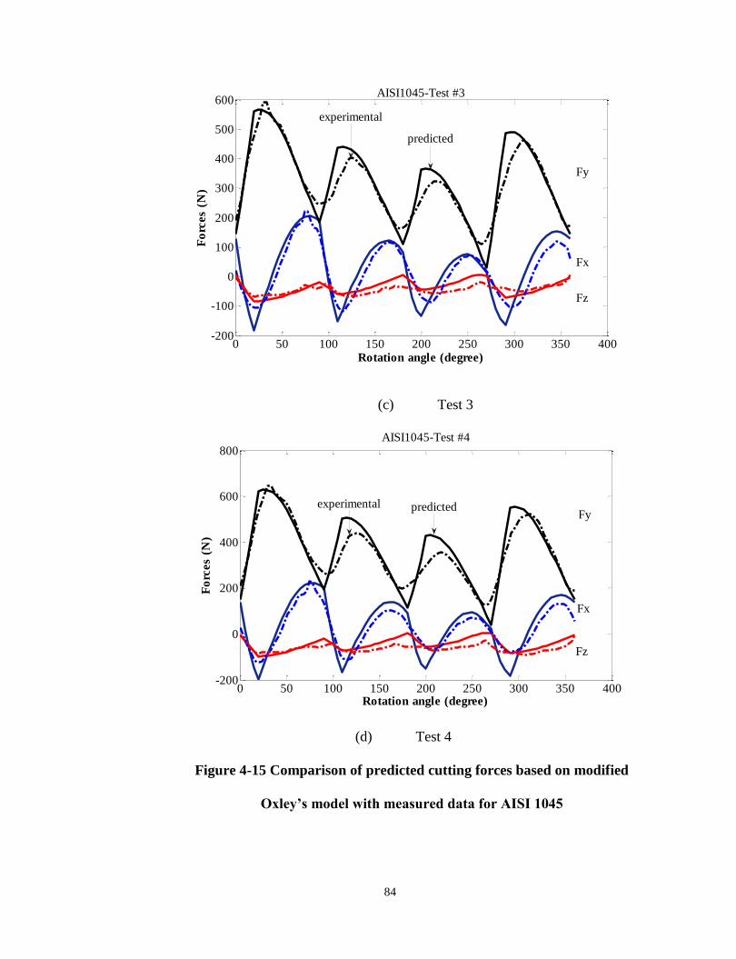
84
(c) Test 3
(d) Test 4
Figure 4-15 Comparison of predicted cutting forces based on modified
Oxley’s model with measured data for AISI 1045
0 50 100 150 200 250 300 350 400-200
-100
0
100
200
300
400
500
600
Rotation angle (degree)
Fo
rces
(N)
AISI1045-Test #3
Fz
Fx
Fy
experimental
predicted
0 50 100 150 200 250 300 350 400-200
0
200
400
600
800
Rotation angle (degree)
Fo
rces
(N)
AISI1045-Test #4
Fz
Fy
Fx
predictedexperimental
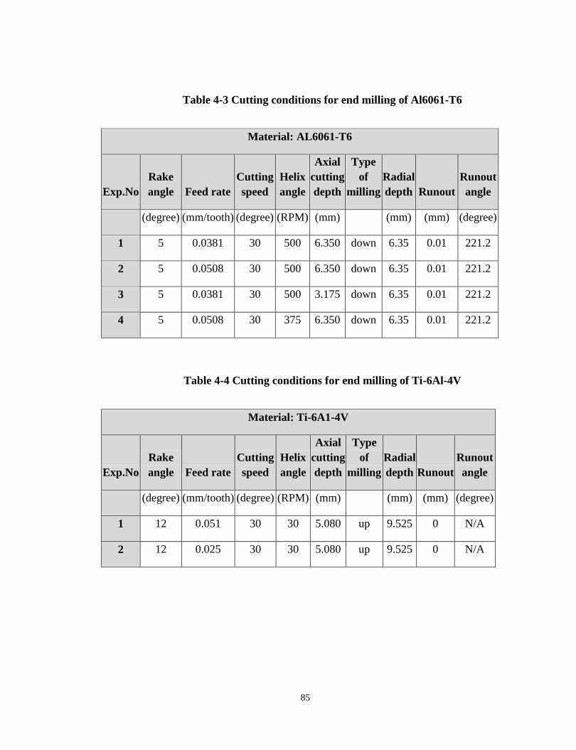
85
Table 4-3 Cutting conditions for end milling of Al6061-T6
Material: AL6061-T6
Exp.No
Rake
angle Feed rate
Cutting
speed
Helix
angle
Axial
cutting
depth
Type
of
milling
Radial
depth Runout
Runout
angle
(degree) (mm/tooth) (degree) (RPM) (mm) (mm) (mm) (degree)
1 5 0.0381 30 500 6.350 down 6.35 0.01 221.2
2 5 0.0508 30 500 6.350 down 6.35 0.01 221.2
3 5 0.0381 30 500 3.175 down 6.35 0.01 221.2
4 5 0.0508 30 375 6.350 down 6.35 0.01 221.2
Table 4-4 Cutting conditions for end milling of Ti-6Al-4V
Material: Ti-6A1-4V
Exp.No
Rake
angle Feed rate
Cutting
speed
Helix
angle
Axial
cutting
depth
Type
of
milling
Radial
depth Runout
Runout
angle
(degree) (mm/tooth) (degree) (RPM) (mm) (mm) (mm) (degree)
1 12 0.051 30 30 5.080 up 9.525 0 N/A
2 12 0.025 30 30 5.080 up 9.525 0 N/A

86
Table 4-5 Cutting conditions for end milling of Al-T7075
Material: T7075 Aluminum alloy
Exp.No
Rake
angle Feed rate
Helix
angle
Spindle
speed
Axial
cutting
depth
Type
of
milling
Radial
depth Runout
Runout
angle
(degree) (mm/tooth) (degree) (RPM) (mm) (mm) (mm) (degree)
1 5 0.052 30 1167 8.900 up 10.16 0 N/A
2 5 0.076 30 1167 8.900 up 10.16 0 N/A
(a) Test 1
0 50 100 150 200 250 300 350 400-200
-100
0
100
200
300
400
500
Rotation angle (degree)
Fo
rces
(N)
AL6061-Test #1
Fz
Fx
Fy
experimental
predicted

87
(b) Test 2
(c) Test 3
0 50 100 150 200 250 300 350 400-200
-100
0
100
200
300
400
500
600
Rotation angle (degree)
Fo
rces
(N)
AL6061-Test #2
Fz
Fx
Fy
experimental
predicted
0 50 100 150 200 250 300 350 400-100
-50
0
50
100
150
200
250
Rotation angle (degree)
Fo
rces
(N)
AL6061-Test #3
predicted
experimental
Fx
Fz
Fy
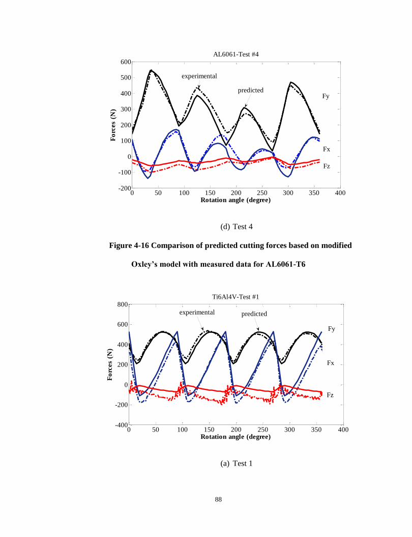
88
(d) Test 4
Figure 4-16 Comparison of predicted cutting forces based on modified
Oxley’s model with measured data for AL6061-T6
(a) Test 1
0 50 100 150 200 250 300 350 400-200
-100
0
100
200
300
400
500
600
Rotation angle (degree)
Fo
rces
(N)
AL6061-Test #4
Fy
Fx
Fz
predicted
experimental
0 50 100 150 200 250 300 350 400-400
-200
0
200
400
600
800
Rotation angle (degree)
Fo
rces
(N)
Ti6Al4V-Test #1
Fy
Fx
Fz
predictedexperimental

89
(b) Test 2
Figure 4-17 Comparison of predicted cutting forces based on modified
Oxley’s model with measured data for Ti6Al4V
(a) Test 1
0 50 100 150 200 250 300 350 400-200
-100
0
100
200
300
400
500
Rotation angle (degree)
Fo
rces
(N)
Ti6Al4V-Test #2
Fx
predictedFy
Fz
experimental
0 50 100 150 200 250 300 350 400-200
0
200
400
600
800
Rotation angle (degree)
Fo
rces
(N)
AL7075-Test #1
Fy
Fx
Fz
predictedexperimental

90
(b) Test 2
Figure 4-18 Comparison of predicted cutting forces based on modified
Oxley’s model with measured data for AL7075
As shown in these helix end milling force profiles, several features can be noticed.
The cutting forces in all three directions increase gradually to the peak values,
instead of jumping directly to the peak. This is due to the effect of the helix angle.
Without helix angle, a specific cutting flute will engage into material at the same
time. Because of the lag angle caused by the helix angle, the cutting flute will
engage into material gradually from the bottom up to the height of the axial depth
of cut. Therefore, the peak force values are reached at the moment when the total
chip thickness contributed by all the elements along the helix flute is the
maximum. The larger the helix angle, the later the peak value be achieved.
0 50 100 150 200 250 300 350 400-400
-200
0
200
400
600
800
1000
Rotation angle (degree)
Fo
rces
(N)
AL7075-Test #2
Fz
Fx
Fy
experimental predicted

91
yF acts constantly in positive direction. This is obvious because the force
components contributed by both cF and rF are all in the positive Y direction
during the whole cutting engagement.
xF oscillates from negative to positive as the flutes engage and disengage. This
feature is contributed to the opposite x components of the cF and rF . When the
cutting flute begins to cut, the direction of cF is perpendicular to the feed
direction, while rF acts in the same direction as the feed. Therefore, xF acts in
the negative feed direction. As the tool rotates, the domination of rF is attained
by cF gradually. It is easy to find that the contribution from cF and rF will
reach the balance at the rotation angle of / 4 , meaning that xF will be zero at
this moment if c rF F . The fact that for most cutting conditions and materials
c rF F is always true makes xF reach zero earlier.
The effect of runout can be seen vividly in all the plots. The first flute experiences
the largest chip thickness and the third flute experiences the smallest. More
importantly, it can be seen that it is the cutting radius difference, not the effective
cutting radius itself that contributes the effect of runout. Referring to the runout
geometry in this experiment, the order of the effective cutting length from high to
low for the four cutting flutes is 1-2-4-3, while the order of peak forces is 1-4-2-3.

92
This fact indicates that the fourth flute experienced larger chip thickness than the
second flute did, although the second flute has a longer effective cutting radius.
The reason is that the second flute has a shorter effective radius than the first one,
so a portion of chip thickness supposed to be left for it is “robbed” by the first
flute. On the other hand, although the fourth flute has a shorter effective length
than the second one, it “enjoyed” a large portion of chip thickness left by the
shortest flute, the third flute. The conclusion could be reached that the radial
runout offset redistributes the share of chip load. The MMR might not be
influenced so much.
All these features discussed above are captured very well by the developed force model.
By using Johnson-Cook material model to represent material behaviour, almost the same
results are achieved.
4.6 Conclusion
In this chapter, an analytical end milling force model was developed and verified. An
analysis of the cutting forces for helix end milling processes was performed and an
application of Oxley‟s orthogonal machining theory to the end milling force prediction
was achieved. The end milling force profile under the condition of cutter offset is able to
be simulated by the model, with the input data of cutting conditions, machine tool
geometry and the work material properties.

93
CHAPTER 5.
PHENOMENOLOGICAL MODELING OF
DEFORMATION DURING METAL CUTTING
Equation Chapter (Next) Section 1
5.1 Introduction
In Oxley's machining theory, the efforts have been made to address work hardening and
thermal softening effects and allow the material to flow continuously through an opened-
up deformation zone. However, the strain, strain rate and temperature were calculated
based on the average values. The distributions of these processing parameters, which are
essential to describe the continuous flow, were not taken into account. In particular, the
hodograph was adopted from the single shear plane model, in which the velocity field
allowing for the continuous deformation was not described, and the issue of velocity
discontinuity has not been resolved. In this chapter, the prediction of various processing
parameters is based on the methodology developed in Chapter 3, while the strain, strain

94
rate and velocity fields in the primary shear zone that allows the continuous deformation
has been analyzed, in an attempt to provide an improved insight into the flow behavior in
the primary shear zone. With the detailed analysis on the boundary conditions of the
velocity and shear strain rate fields, the thick “equidistant parallel-sided” shear zone
model was revisited. A more realistic nonlinear shear strain rate distribution has been
proposed under the frame of non-equidistant primary shear zone configuration, so that all
the boundary conditions can be satisfied.
5.2 Velocity, strain and strain rate during chip formation
In Oxley's parallel-sided shear zone model shown in Figure 2-10, the shear zone is
bounded by the lower boundary CD where the deformation starts and upper boundary EF
where the deformation ends. An approximation was made where CD and EF are assumed
to be parallel to and equidistant from AB. The hodograph utilized in the analysis was the
same as that in single shear plane model without considering the material continuity. In
addition the total shear strain at upper boundary EF was calculated in a way identical to
that proposed by Merchant [2] and the strain at AB was taken as one half of the total
strain , as shown in Equation (2.27). This result is the direct consequence of the
equidistance assumption and the absence of the strain distribution expression across the
primary shear zone.

95
Based on the experimental data, Oxley [10] showed that the strain rate distribution is a
bell-shaped curve through the primary shear zone and the maximum shear strain rate
occurs at AB. However, the strain rate distribution was not formulated or utilized in the
analysis and instead the shear strain rate at AB is used and calculated by Equation (2.28).
Based on the engineering plasticity, several researchers reevaluated the orthogonal metal
cutting mechanics in the primary shear zone [35-38]. In their studies, the coordinate
system is commonly set based on the shear angle, as shown in Figure 5-1, where the x
direction is set along the shear zone boundaries and the y direction is perpendicular.
Figure 5-1 Simplified non-equidistance primary shear zone

96
Since the boundaries CD and EF are assumed to be slip lines, Geiringer‟s Equation
holds:
0x ydV V d (5.1)
Because the slip lines are simplified to be straight, Equation (5.1) implies that is
constant along x direction, or
0xV
x
(5.2)
The continuity of incompressible plastic materials requires
0yx
VV
x y
(5.3)
Equation (5.2) and (5.3) imply that the velocity component normal to the shear plane AB
is constant across the parallel-sided shear zone and therefore all the analysis in the
primary shear zone can be considered as one dimension. For a given cutting speed , the
entry and exit boundary conditions for the velocity field can be obtained.
1 0
2
cos
sin tan
sin
x x y
x x y h
y y
V V U
V V U
V V y U
(5.4)

97
The velocity discontinuity is defined as the difference between and [37]:
*
2 1
cos
cosx x xV V V U
(5.5)
It should be noted that equals in magnitude. Comparing Equation (5.5) and (2.28),
it also can be seen that
in Eq. (2) is actually the mean shear strain rate of the primary
shear zone, since the mean shear strain rate
is expressed as:
*
2 1x x xm
V V V
h h
(5.6)
In this study, it should be noticed that the simple shear is assumed to occur along parallel
planes and therefore the main frame remains unchanged during plastic deformation. Thus,
the shear strain rate can be related to the shear strain and velocity, as shown in Equation
(5.7) and (5.8) respectively.
y x x
V V dV
x y dy
(5.7)
y
d dy dV
dt t y dt dy
(5.8)
Substituting Equation (5.7) into Equation (5.8) and integrating with respect to y, the
relation between velocity and shear strain field can be expressed such that:
1
cotx
y
y V yV
(5.9)

98
As can be seen from Equation (5.4), as long as the shear angle is greater than the rake
angle, the sign of are opposite, indicating that there must be a plane, in the
primary shear zone, at which the tangential velocity is zero. This plane is the potential
sliding plane [37] and it is therefore reasonable to assume it as the main shear plane, at
which the discontinuity of the shear stress and velocity could take place and the shear
strain rate is the maximum. Many researchers observed from quick stop analysis that the
primary shear zone is divided by the main shear plane into two unequal regions. The
lower region (from CD to AB) is wider than the upper region (from AB to EF). The
detailed review can be found in the work by Tounsi, et al. [35]. Astakhov, et al. [37]
further realized that in the lower wide region the velocity ratio changes with lower rate,
but in the upper narrow region it changes with higher rate. They also observed based on
experimental data that the non-uniform distribution of the tangential velocity in the
primary deformation zone is proportional to at moderate cutting speed.
From the above analysis, if is defined as the proportion of the lower part to the total
width of the deformation zone, the boundary conditions of the velocity and shear strain
rate fields in the primary shear zone are as follows:
1) The primary shear zone is unequally divided by the main shear plane AB (
).

99
2) The quantities defining plastic deformation depends only on y, the direction
perpendicular to the main shear plane.
3) The tangential velocity is and at lower and upper deformation boundaries
respectively (Equation (5.4)).
4) The tangential velocity is zero at main shear plane AB.
0x y hV
(5.10)
5) The shear strain rate at main shear plane AB is the maximum and is zero at lower
and upper boundaries.
ABy h
(5.11)
0
0y
(5.12)
0y h
(5.13)
6) Since the material particles move toward the primary shear zone with constant
speed, the change rate of the velocity and the corresponding shear strain rate are
zero before the lower boundary CD is reached. Similarly, after passing through
the upper boundary EF, the strain rate of the particles reduces to zero again. If
the strain rate distribution is assumed to be represented by a smooth differentiable
curve across the entire primary shear zone from CD to EF (including both inner
sides and outer sides), there must be an extremely thin buffer zone around CD
and EF, in which the gradient of the shear strain rate with respect to y is zero. In

100
this study, the locations around CD and EF that the gradient of the shear strain
rate reaches zero are defined as lower and upper boundaries respectively.
Furthermore, the assumed differentiable nature of the curve leads to the fact that
the gradient of the shear strain rate with respect to y is also zero at the main shear
plane AB where the shear strain rate reaches the maximum, i.e.,
0y h
d
dy
(5.14)
0
0y
d
dy
(5.15)
0y h
d
dy
(5.16)
7) A fourth order polynomial curve in terms of y and h could describe the velocity
distribution in the primary shear zone for moderate cutting speed [37] .
According to these characteristics and boundary conditions, the pattern of velocity and
shear strain rate distribution may be illustrated in Figure 5-2. Based on these conditions
and considering a 4th
order polynomial curve is possible to describe the velocity field for
moderate cutting speeds, the following piecewise strain rate distribution is proposed.
2 2
2 2
Dy y Ehy + Fh 0
γ =
d h - y y + ehy + fh
y h
y h h
(5.17)

101
In which are coefficients that need to be determined.
It can be seen Equations (5.12) and (5.13) are satisfied by Equation (5.17). The gradient
of shear strain rate through the primary shear zone can be expressed as:
2 2
2 2
3 2 0
3 2 1
D y Ehy Fh y hd
dyd y e hy f e h y h h
(5.18)
Considering the boundary conditions of Equation (5.4), the velocity field can be obtained
by the spatial integration of shear strain rate.
4 3 2 2
1
0
2
2
2 2
1 1 1
4 3 2
3 2 41
12 1 2 6
h
x
xh
x
h
dy V D y Ehy Fh y
V
y e hydy V d h y
e f h
(5.19)

102
Figure 5-2 Demonstration of the distribution of tangential velocity and shear
strain rate in the primary shear zone
For h , in order to satisfy Equation (5.15),
0F (5.20)
In order to satisfy Equation (5.14)
3 2F E (5.21)

103
Substituting Equation (5.20) into (5.21),
3
2E (5.22)
In order to satisfy Equation (5.11),
3 3
2 3
AB h DE
D h
(5.23)
From Equations (5.21) and (5.23), the constants can be expressed in terms of and h,
as shown in Equation (5.24).
3 3
2 ABDh
(5.24)
In order to satisfy Equation (5.10), the shear strain rate at main shear plane AB can be
obtained.
12 xAB
V
h
(5.25)
Similarly, from conditions(5.11),(5.14) and (5.16) for h , coefficients
can be obtained.

104
33
2
1
ABdh
(5.26)
3 1
2e
(5.27)
3 1
2f
(5.28)
Satisfying Equation (5.10) by Equation (5.19), the shear strain rate at AB can also be
calculated as
22
1
xAB
V
h
(5.29)
The combination of Equation (5.25) and (5.29) lead to the expression of .
1 1
*
1 2
x x
x x x
V V
V V V
(5.30)
Considering
and , and
can finally be expressed as
cos cos
cos
(5.31)

105
*
2 2xAB m
V
h (5.32)
Finally, replacing in Equations (5.17) and (5.19), shear strain rate and
velocity fields can be obtained, as shown in Equations (5.33) and (5.34)
2
3 3
2
33
3 2 0 h
3 2 h h
1
AB
AB
y h yy
h
y
h y h h yy
(5.33)
4 3 4 4
1 4 4
4 3 2 2 3 3
2 44
2 0
2 2 6 2 6
1
x
x
x V
y hy hV y h
h
V yy h h y h y h h y
V A y h hh
(5.34)
where
3 2
4
4 6 2
1VA
(5.35)

106
Using the velocity distribution in Eq. (20) the shear strain distribution in Eq. (11) can be
determined and the corresponding shear strain at the main shear plane can be given by:
cotAB EFy h
(5.36)
Figure 5-3 shows the effect of shear angle on the proportion factor for different values of
rake angle. From the illustrated results, in order to make the main shear plane right at the
middle of the shear zone a combination of large negative rake angle and large shear
angle must occurred. However, this circumstance could hardly happen since cutting
tools with large negative rake angle result in the severe plastic deformation leading to
large chip ratio and therefore small shear angle. On the other hand, could be equal to or
even greater than one if a large positive rake angle is used and very small shear angle
occurred simultaneously. However, this situation is also unrealistic because large shear
angles are always the consequences of using cutting tools with large positive rake angles,
at least when continuous chip formation is assumed. Therefore, from the above analysis,
always falls into the range between 0.5 and 1. This observation is in agreement with
reported experimental observations [35] that the entry zone (from CD to AB) was found
to be wider than the exit zone (from AB to EF).

107
Figure 5-3 Primary shear zone proportion
Figure 5-4~Figure 5-6 show the distributions of the shear strain rate, tangential velocity
and the shear strain across the shear zone for different values of primary shear zone
thickness. One can see from the illustrated results that the proportional factor,
when and , which is unrealistic. In a more realistic case for shear angle
( when cutting with a zero rake, ) the obtained proportional factor
, indicating that the main shear plane AB is closer to the upper deformation
boundary and implying a higher rate of velocity changes in the upper region. This is in
accordance with the experimental observation in [37]. Also, It can be seen from these
figures that for the same total shear strain, the thickness of the primary shear zone (or )
determines how fast the plastic deformation process proceeds. The thinner the primary
shear zone thickness, the faster the progress of the deformation, ie. higher strain rate.
-0.3
0.0
0.3
0.5
0.8
1.0
1.3
1.5
0 20 40 60 80 100
Pro
po
rtio
n o
f th
e P
SZ
(λ)
Shear angle φ (degree)
=-20° =-10° =0° =10° =20°
AB is in the middle of

108
(a) Asymmetric distribution
(b) Symmetric distribution
Figure 5-4 Shear strain rate distribution through the primary shear zone
0
50
100
150
200
250
300
350
400
450
-40 -30 -20 -10 0 10 20
shea
r st
rain
ra
te (
10
00
/S-1
)
Distance from the shear plane AB (μm)
h=20 m
h=30 m
h=50 m
U=200 m/min φ=30O
α=-5O
λ=0.7
AB
0
100
200
300
400
500
600
-30 -20 -10 0 10 20 30
shea
r st
rain
ra
te (
10
00
/S-1
)
Distance from the shear plane AB (μm)
h=20 m
h=30 m
h=50 m
U=200 m/min φ=40O
α=-10O
λ=0.5
AB

109
(a) Asymmetric distribution
(b) Symmetric distribution
Figure 5-5 Tangential velocity distribution through the primary shear zone
-3.5
-3
-2.5
-2
-1.5
-1
-0.5
0
0.5
1
1.5
-40 -30 -20 -10 0 10 20
Ta
ng
enti
al
Vel
oci
ty (
m/s
)
Distance from the shear plane AB (μm)
h=20 m
h=30 m
h=50 m
U=200 m/min φ=30O
α=-5O
λ=0.7
AB
-3
-2
-1
0
1
2
3
-30 -20 -10 0 10 20 30
Ta
ng
enti
al
Vel
oci
ty (
m/s
)
Distance from the shear plane AB (μm)
h=20 m
h=30 m
h=50 m
U=200 m/min φ=40O
α=-10O
λ=0.5
AB

110
(a) Asymmetric distribution
(b) Symmetric distribution
Figure 5-6 Shear strain distribution through the primary shear zone
0.00
0.50
1.00
1.50
2.00
2.50
3.00
-40 -30 -20 -10 0 10 20
Sh
ear
stra
in
Distance from the shear plane AB (μm)
h=20 m
h=30 m
h=50 m
U=200 m/min φ=30O
α=-5O
λ=0.7
AB
0.00
0.50
1.00
1.50
2.00
2.50
3.00
-30 -20 -10 0 10 20 30
Sh
ear
stra
in
Distance from the shear plane AB (μm)
h=20 m
h=30 m
h=50 m
U=200 m/min φ=40O
α=-10O
λ=0.5
AB

111
5.3 Results and discussion
In this chapter, Oxley‟s machining theory has been modified to consider the shear strain
and strain rate distribution across the primary shear zone. The presented analysis based
on the velocity and strain field for the incompressible material reveals that the location of
the main shear plane is not right in the middle of the primary shear zone, but can be
related to the material properties and cutting conditions. In this section, the comparison
will be made between the current and Oxley‟s results when predicting process
parameters such as cutting forces, chip thickness and secondary shear zone thickness.
The work materials used for comparison in this work are 0.20% carbon steel and AISI
1045 steel. The experimental data for 0.20% carbon steel is adopted form [10] and that
for AISI 1045 steel is adopted from [39].
Figure 5-7 and Figure 5-8present the predicted and measured machining forces and chip
thickness for 0.20% carbon steel. The marks with the solid fill are the data when built-
up-edge were observed. It can be seen that there is no significant difference between the
current and Oxley‟s predictions. This may be explained by the fact that the cutting forces
are determined by both work hardening and thermal softening effects. With the “unequal
distance” primary shear zone, the predicted shear strain, shear strain rate and
temperatures in the current study are all higher than that by Oxley‟s original method. So
that the resultant effect of work hardening and thermal softening makes the results
similar. However, the uncertainty about the location of the main shear plane is eliminated

112
in the current work. Instead of , the predicted location of the main shear plane is
closer to the upper boundary of the primary shear zone, which was discussed earlier, and
it tends to move towards the lower boundary as the cutting speed increases, as shown in
Figure 5-9.
Figure 5-9 (a) presents the predicted thickness of the primary shear zone. Oxley's
predictions are quite similar to that in the current study; they both decrease with the
increase in cutting speed and uncut chip thickness. However, the uncertainty about the
location of the main shear plane is eliminated in the current work, as can be seen in
Figure 5-9(b) that varies with the cutting speed and uncut chip thickness. The increase
in both cutting speed and the uncut chip thickness decreases , indicating that the
deformation process will be more symmetric when cutting material with high feed and
high cutting speed.
(a) Cutting force
0
1000
2000
3000
4000
5000
6000
0 100 200 300 400 500
Cu
ttin
g F
orc
e (N
)
Cutting Speed (m/min)
t1=0.5mm
t1=0.25mm
t1=0.125mm
Oxley's prediction
Current prediction
Experiment

113
(b) Thrust force
Figure 5-7 Machining forces for 0.20% carbon steel:
Figure 5-8 Chip thickness for 0.20% carbon steel:
0
500
1000
1500
2000
2500
3000
3500
4000
4500
5000
0 100 200 300 400 500
Th
rust
Fo
rce
(N)
Cutting Speed (m/min)
t1=0.5mm
t1=0.25mm
t1=0.125mm
Oxley's prediction
Current prediction
Experiment
0
0.5
1
1.5
2
2.5
0 100 200 300 400 500
Ch
ip t
hic
kn
ess
(mm
)
Cutting Speed (m/min)
t1=0.5mm
t1=0.25mm
t1=0.125mm
Oxley's prediction
Current prediction
Experiment

114
(a) Thickness of the primary shear zone
(b) Proportion factor ( ) of the primary shear zone
Figure 5-9 Predicted thickness and the proportion factor of the primary
shear zone for 0.20% carbon steel:
-0.1
6E-16
0.1
0.2
0.3
0.4
0.5
0.6
0 100 200 300 400 500
PS
Z t
hic
kn
ess
(mm
)
Cutting Speed (m/min)
t1=0.125mm
t1=0.5mm
t1=0.25mm
Oxley‟s prediction
Current prediction
0.7
0.75
0.8
0.85
0.9
0.95
1
0 100 200 300 400 500
Pro
po
rtio
n f
act
or
of
PS
Z (
l)
Cutting Speed (m/min)
t1=0.5mm
t1=0.25mm
t1=0.125mm

115
Figure 5-10 presents the thickness of the secondary shear zone at various uncut chip
thickness. As can be seen, the predicted values in the current work are lower than that
predicted by Oxley's model when cutting speed is low and they tend to coincide at high
cutting speeds, particularly for the high feed rate. The difference between the current and
previous predicted results can be explained by the dependence of the thickness of the
secondary shear zone on the severeness of the further shear at the chip-tool interface. The
more severe the shearing, the thinner the secondary shear zone. In order to balance the
resultant force transmitted from the primary shear zone, the shear stress at the chip-tool
interface and on the main shear plane are interrelated, and is affected by the
combined effects of work hardening and thermal softening. Since in the current
study, the predicted shear strain, strain rate and temperature at main shear plane are
higher than Oxley‟s prediction. The lower cutting speed results in the lower temperature,
so that the effect of work hardening predominates on the main shear plane. Therefore,
when cutting speed is low, the currently predicted shear stress is higher and the
corresponding thickness of the secondary shear zone is lower. When the cutting speed
increases, the resulted high temperature counteracts the effect of work hardening and
makes the magnitude of similar to that predicted by Oxley. Consequently,
compared to Oxley‟s prediction, the thickness of the secondary shear zone is lower in the
current study, especially at lower cutting speeds. However, it is important to note that the
current prediction shows improved agreement with the mean value of the experimental
data.

116
(a)
(b)
0
0.01
0.02
0.03
0.04
0.05
0.06
0.07
0.08
0 50 100 150 200 250 300 350 400 450
SS
Z t
hic
kn
ess
(mm
)
Cutting Speed (m/min)
Oxley's prediction
Current prediction
Experiment
0
0.02
0.04
0.06
0.08
0.1
0.12
0.14
0 50 100 150 200 250 300 350 400 450
SS
Z t
hic
kn
ess
(mm
)
Cutting Speed (m/min)
Oxley's prediction
Current prediction
Experiment

117
(c)
Figure 5-10 Secondary shear zone thickness for 0.20% carbon steel:
Figure 5-11shows the predicted shear strain rate, shear strain and velocity distributions
across the primary shear zone. As can be seen in Figure 5-11(a), the location of the main
shear plane AB is shifting towards the lower boundary of the plastic deformation zone
when cutting speed increases. Moreover, not only the average magnitude, but also the
gradient of the shear strain rate and tangential velocity is increased, reflecting the fact
that the time left for the gradual plastic deformation is less during cutting with higher
speed and the chip formation process tends to be localized at the main shear plane. On
the other hand, the total shear strain at the exit boundary decreases with the increase in
the cutting speed, as shown in Figure 5-11(b). In fact, the total shear strain is the
accumulation of the local shear strains on all the layers across the plastic deformation
0
0.02
0.04
0.06
0.08
0.1
0.12
0.14
0.16
0.18
0.2
0 50 100 150 200 250 300 350 400 450
SS
Z t
hic
kn
ess
(mm
)
Cutting Speed (m/min)
Oxley's prediction
Current prediction
Experiment

118
zone. The lower cutting speed provides more time and space for the work material to
respond to the external force, as can be seen in Figure 5-11(c). As the result, the width of
primary shear zone is increased by the decrease in the cutting speed, indicating that more
material particles are involved in the plastic deformation and contribute shear strains to
the total shear strain. Consequently, the developed strain energy is larger and the cutting
energy needed to remove the material is higher. This can be reflected from the higher
machining forces at lower cutting speeds.
(a) Shear strain rate distribution
0
1,000
2,000
3,000
4,000
5,000
6,000
0 0.2 0.4 0.6 0.8 1 1.2
Sh
ear
stra
in r
ate
(S
-1)
Nondimensional distance from the entry boundary of the primary
shear zone
U=100 m/min
U=200 m/min
U=400 m/min
AB
Entry boundary Exit boundary

119
(b) Tangential velocity distribution
(c) Shear strain distribution
Figure 5-11 Predicted shear strain rate, shear strain and velocity
distributions across the primary shear zone for 0.20% carbon steel:
0.00
0.50
1.00
1.50
2.00
2.50
3.00
3.50
4.00
4.50
-3.5 -3 -2.5 -2 -1.5 -1 -0.5 0 0.5 1
Sh
ear
stra
in
Distance from the shear plane AB (mm)
U=100 m/min
U=200 m/min
U=400 m/min
AB
-7
-6
-5
-4
-3
-2
-1
0
1
2
-3.5 -3 -2.5 -2 -1.5 -1 -0.5 0 0.5 1
Ta
ng
enti
al
Vel
oci
ty (
m/s
)
Distance from the shear plane AB (mm)
U=100 m/min
U=200 m/min
U=400 m/min
AB

120
Furthermore, another set of data was selected from the experimental work done by
Ivester et al [39], to evaluate the effect of modifications under various cutting conditions.
The cutting conditions are listed in Table 5-1. In their work, the orthogonal cutting tests
were conducted form 4 laboratories using the same cutting tools. The upper bound (solid
line) and the lower bound (dash line) of the measured forces are shown in Figure 5-12. It
can be seen again that no distinguishable difference can be found between two models.
One can see that the predicted cutting forces basically fall into the boundaries. However,
most thrust forces are underestimated. This may be attributed to the assumption of the
perfectly sharp tool applied in the current study.
Table 5-1 Orthogonal Cutting Conditions For AISI 1045 (w=1.6 mm) [39]
Test
V
(m/min)
t1
(mm)
α
(degree)
1 200 0.15 -7
2 200 0.15 5
3 200 0.30 -7
4 200 0.30 5
5 300 0.15 -7
6 300 0.15 5
7 300 0.30 -7
8 300 0.30 5

121
(a) Cutting force
(b) Thrust force
Figure 5-12 Comparison of predicted machining forces with experimental
data [39] for AISI 1045 steel:
300
500
700
900
1100
1300
1500
1 2 3 4 5 6 7 8
Cu
ttin
g F
orc
e (N
)
Test Number
Oxley prediction
Current prediction
100
200
300
400
500
600
700
800
900
1000
1100
1 2 3 4 5 6 7 8
Th
rust
Fo
rce
(N)
Test Number
Oxley prediction
Current prediction

122
5.4 Conclusion
In this chapter, an attempt has been made to modify Oxley‟s machining theory by
considering the effect of shear strain, strain rate distributions. A more realistic bell-
shaped strain rate distribution through the primary shear zone was proposed in an
attempt to satisfy all the velocity field boundary conditions. The proportion parameter ( )
of the primary shear zone was determined as part of the solution, so that Oxley‟s “equi-
distance” assumption was eliminated. The effect of the modification made to Oxley‟s
model was evaluated in terms of machining forces, chip thickness and secondary shear
zone thickness. It has been found that the main shear plane, at which the shear strain rate
reaches the maximum, hardly locates at the middle of the primary shear zone in the
moderate range of cutting speed. Instead, it is closer to the upper boundary of the plastic
deformation zone and dependant on where the tangential velocity of work material
particle changes direction. Although the modified model predicts higher strain, strain rate
and temperature at the main shear plane, the machining forces are quite similar to that by
Oxley‟s original model. However, this coincidence is encouraging since the modified
model is more phenomenological and several uncertainties are eliminated from the
previous model.

123
CHAPTER 6.
IDENTIFICATION OF MATERIAL
CONSTITUTIVE EQUATION FOR METAL
CUTTING Equation Chapter (Next) Section 1
6.1 Introduction
With the development of computer technology, the numerical methods, such as Finite
Difference and Finite Element Analysis have been widely applied to the simulation of
metal cutting processes. One of the obstacles that hinder the further application of CAE
technology is the successful identification of the set of parameters in the material
constitutive model. Furthermore, plasticity based analytical modeling of metal cutting
process, as the one in the current study, highly depends on the accuracy of material
model as well. Therefore, the accurate identification of the material parameters under the
conditions similar to that encountered in metal cutting is crucial. Split Hopkinson
Pressure Bar (SHPB) tests have been commonly used to obtain material constants at

124
various strain rate and temperature levels. However, much higher strain rate are
commonly observed in real metal cutting process, and due to the extremely high heating
rate during chip formation, there is no enough time for complete phase transformation,
anneal softening, age hardening, or even blue brittleness effects to occur[40].
Inverse analysis applies optimization techniques to identify the material parameters by
minimizing a particular norm of the difference between the calculated and experimental
machining data, in an attempt to reach the extreme conditions (high strain, strain rate and
temperature) encountered in metal chip formation process. Shatla et al [41] developed a
methodology using “OXCUT” and 2D orthogonal slot milling test to obtain modified
Johnson-Cook parameters. A multi-directional Downhill Simplex Algorithm was chosen
to minimize the sum of deviations between the measured and calculated cutting and
thrust forces. This methodology was further improved by Sartkulvanich et al [42] by
measuring the thickness of primary and secondary shear zone thickness. The Johnson-
Cook model for low carbon steels was modified to take the blue brittleness effect into
account. Chandrasekaran and M‟Saoubi [43] used milling test to obtain Johnson-Cook
constants as well. In their study, the data from SHPB tests was applied as starting point
for least square search. Instead of cutting and thrust forces, the shear stress along the
primary deformation zone was used to create the objective function, making the inverse
analysis at the tool-chip interface unnecessary. Lei et al [44] calculated strain rate based
on a triangular shear zone. The shear plane temperature was measured with the infrared
camera through a small opening in the shield placed in front of the cutting tool, and the

125
angle formed between upper/lower boundary and the shear plane AB was measured from
a photograph of the microstructure associated with the side of the chip. Tounsi et al [35]
re-evaluated the velocity field, stress and strain states in the primary shear zone based on
the plastic incompressibility. In their study, the primary shear zone was assumed not
equi-distant and the thickness was assumed one half of the feed rate. An expression was
derived to define the portion of primary shear zone in terms of shear angle and tool rake
angle. Based on the developed strain, strain rate and the temperature along shear plane
AB, a least-square approximation technique was applied to determine the Johnson-Cook
constants. Pujana et al [40] applied inverse analysis to the secondary shear zone. With
the measured tool-rake face temperature and the thickness of secondary shear zone, the
Johnson-Cook constants were tuned based on the experimental characterization results.
Ozel and Zeren [45] applied Gauss-Newton algorithm to obtain Johnson-Cook constants
by utilizing measured forces and chip thickness obtained through orthogonal cutting tests.
In their methodology, the assumption of the primary shear zone thickness was eliminated
and the shear strain rate constant was obtained by the inverse analysis of Oxley‟s
theory.
In these optimization methods the proper starting points are needed. Improper starting
points could lead to local optimum instead of global optimum. In order to overcome this
obstacle, in this Chapter, an attempt has been made to develop a Genetic Algorithm for
the identification of Johnson-Cook parameters under the conditions encountered in metal

126
cutting process. The methodology is based on the methodology of the primary shear zone
developed in the previous chapter, in conjugation with orthogonal cutting tests.
6.2 Inverse analysis in the primary shear zone
First of all, the cutting force , thrust force and chip thickness should be measured
from experiment. The shear angle can then be determined.
1
1 2
1
2
cos
tan
1 sin
t
t
t
t
(6.1)
Secondly, the shear strain, shear strain rate and temperature can be calculated with
equations (5.36), (5.32) and (2.32), and substituted into Johnson-Cook equation (3.1), to
obtain the calculated flow stress . 0C has to be known in prior to calculate shear strain
rate. From the slip line field analysis described in chapter 3, 0C can be expressed in terms
of equivalent flow stress ,
0
3
2
n
ABA B n
AB AB
A BC P P
n
(6.2)
where AP can be calculated from Equation (3.12) and BP can be derived based on the
known experiment data.

127
1
2sinsin cosB A c tP P F F
t w
(6.3)
On the other hand, the average flow stress on the shear plane can be obtained by force
relations with the measured data,
exp
1
3sincos sinc tF F
wt
(6.4)
Finally, in order to identify the five flow stress parameters, an error function may be built
to be minimized through a certain optimization algorithm, as shown in Equation(6.5).
2
1
1, , , , min 1
Ncal
i AB
A B n C mN
(6.5)
To carry out the minimization of Equation (6.5), a Genetic Algorithm was developed to
carry out the minimization and will be introduced in the next section.
6.3 Development of Genetic Algorithm for the system identification
Genetic algorithm (GA), first developed by Holland [46], is a selective random search
algorithm designed to achieve a global optimum within a large space of solutions. It
resembles the process of natural selection in search for better characteristics within a
changing population. GA has been used as efficient optimizers and employ the concept

128
„survival of the fittest‟ among string structures. The initial solutions of GA algorithm are
usually randomly generated and form the current generation. The current generation goes
through the following procedure and generates new solutions. The procedure is then
repeated until the certain termination criteria are satisfied.
6.3.1. Encoding
The GA starts with a randomly generated population of n individuals and l-bit
chromosomes, as demonstrated in Figure 6-1.
Figure 6-1 Chromosome strings arrangement
In this study, the chromosome length for each variable is 30 and therefore each
individual in the current population is represented by a 150-bits string, in order to
account for five Johnson-Cook parameters.

129
6.3.2. Selection scheme
Roulette selection combined with elitism was adopted as the selection scheme so that the
improvement for each generation can be achieved without sacrificing population
diversity. In this study, an elitist strategy is executed by allowing top 5% of parent
solutions to propagate directly to the new generation. The left M individuals are put into
the selection pool. For each individual, the probability of being chosen as a parent
depends on the fitness , which can be calculated by the following equations.
max, , , , , , , ,i iF A B n C m F g A B n C m (6.6)
, , , ,
, , , ,
i
i
F A B n C mP i
F A B n C m
(6.7)
1
1M
i
P i
(6.8)
In which M is the population size, is the objective value of the ith individual and
is the maximum objective value in the current solution space. Based on the fitness
value, the individuals are selected by spinning the Roulette wheel. The individual with
higher fitness value has higher possibility to be selected for further genetic operation.
Therefore, it is possible and very common that a certain individual is chosen more than
one time. After the selection, the mating pool of M solutions is established and ready to
go through the crossover and mutation operations.

130
6.3.3. Mutation and crossover operator
Crossover is the mechanism of generating new solutions by mating selected parent. The
number of parent solutions selected for the operation is commonly governed by a user
defined crossover rate Pc. Single point-crossover, Multipoint-crossover, and Uniform-
crossover are widely applied strategies. In this study, the Single point-crossover and
Multipoint-crossover operation is integrated in such a manner, as shown below, in order
to improve the offspring diversity.
For the given two parent solutions represented by binary strings, for instance,
Parent1: 1 1 1 0 1 0 0 1 1 0 1 1 1 1 0 1 1 0 1 0 0 1
Parent2: 0 1 0 0 1 0 1 1 1 0 1 1 0 1 0 0 1 0 1 0 0 1
two crossover points, 5 and 10 are randomly selected,
Parent1:
1 1 1 0 1 0 0 1 1 0 1 1 1 1 0 1 1 0 1 0 0 1
Parent2:
0 1 0 0 1 0 1 1 1 0 1 1 0 1 0 0 1 0 1 0 0 1
two offspring solutions can then be generated by exchanging the sub-stings between the
two crossover points.

131
Offspring1:
1 1 1 0 1 0 1 1 1 0 1 1 0 1 0 1 1 0 1 0 0 1
Offspring2:
0 1 0 0 1 0 0 1 1 0 1 1 1 1 0 0 1 0 1 0 0 1
However, if the two randomly selected crossover points are very close to each other, say,
3 and 5, we can see that the two generated offspring are exactly same as the two parents.
Parent1:
1 1 1 0 1 0 0 1 1 0 1 1 1 1 0 1 1 0 1 0 0 1
Parent2:
0 1 0 0 1 0 1 1 1 0 1 1 0 1 0 0 1 0 1 0 0 1
In order to avoid the redundancy, if the space of the two crossover points is less than 5,
another random number is selected between them and the Single point-Crossover
operator will be used. Therefore, in this example, the two offspring become
Offspring1:
1 1 1 0 1 0 1 1 1 0 1 1 0 1 0 0 1 0 1 0 0 1
Offspring2:
1 1 1 0 1 0 1 1 1 0 1 1 0 1 0 0 1 0 1 0 0 1
In GA, mutation is the random process of selecting one element of the chromosome and
replacing it with a randomly generated gene. Usually, mutation is performed as a
background parameter with very low probability. Mutation guarantees that the

132
probability of search at any given area is never zero. Moreover, it provides an
opportunity of recovering good qualities lost by other genetic operations. The probability
of mutation, Pm, is usually ranged between 0.001-0.01 [47]. In the current study, the
multi-point mutation was used. In order to achieve computing efficiency, the
„simultaneous operation‟ was performed instead of traditional „line-by-line operation‟.
That is, generate i j numbers between 0 and 1; compare each number with mutation
rate Pm; if it is less than Pm, binary integer (BIN) with the same index becomes (1-BIN).
A demonstration is shown in Figure 6-2.
Figure 6-2 Demonstration of multi-point mutation

133
6.3.4. Terminating criteria
Since GA is a stochastic search method, it is very difficult to assign convergence criteria.
Terminate criteria are usually forced into a GA program by 1) specifying maximum
number of generations; 2) terminating if no improvement occurs in last certain number of
generations and 3) terminating if a solution is found whose objective function value or a
user- designed error function value is below a predefined value. The third criterion saves
unnecessary computation time when the algorithm can rapidly reach the global optima
and therefore was adopted in this study. The error between experimental data and the
calculated results is defined in Equation (6.9)
exp
1 exp
1i i
NAB
ii
eN
(6.9)
The program is terminated when e , meaning that the error is smaller than 5%. A
simplified flow chart for the identification process is shown in Figure 6-3.

134
Figure 6-3 Flow chart of identification of Johnson-Cook parameters using
genetic algorithm

135
6.4 Results and discussions
The experimental data used by Ozel and Zeren [45] to identify the Johnson-Cook
constants for AISI 1045 steel (as shown in Table 6-1) was adopted in this study, as the
input to obtain JC parameters under the conditions of metal cutting.
The operation parameters used in the GA algorithm is given in Table 6-2. One of the
attractive GA characteristics is to achieve global optimum without setting starting points.
In most previous studies, the JC parameters obtained from SHPB test were adopted as
the reference to set starting points. In the current study, three tests base on different
searching scheme were carried out in an attempt to examine the effectiveness of the
developed algorithm.
1) SHPB based: The searching ranges for each parameter were set based on SHPB
test from [48].
2) Reasonable constraint: The searching ranges were reasonably extended without
sacrificing the physical significance of each parameter.
3) No constraint: The searching ranges were set extremely large so that it can be
considered as constraint-free for each parameter.

136
The obtained JC parameters for AISI 1045 in the above three cases, along with those
obtained by Ozel and Zeren [45] and Jasper et al [48] are listed in Table 6-3 and Table
6-4 respectively.
The developed GA algorithm was found very efficient to achieve convergence. Figure
6-4 shows the error defined by Equation (6.9) for each generation. In the developed
MATLAB code, the concept of “parallel computation” was fully utilized and therefore
the large population size can be applied without losing much computing efficiency. Due
to the large population size, the error (5.8%) is acceptable even for the first generation.
Because of the “elitism” used in the selection scheme, the improvement for each
generation compared to the previous one was guaranteed. Under the terminating criterion
discussed in the previous section, the global optimum was found less than 50 generations
and the corresponding computing time was about 3 seconds when tested on the
LENOVO T500 laptop computer.
Figure 6-4 Error of the best result for each generation
5 10 15 20 25 30 35 40 45 50
5
5.2
5.4
5.6
5.8
6
Number of Generations
Err
or
(%)

137
Table 6-1 Experimental data of orthogonal cutting of AISI1045 for the
identification of JC parameters [45]
Test V (m/min) t1 (mm) t2 (mm) FC (N) Ft (N) ϕ (degree)
1 100 0.125 0.40 1400 1300 16.9
2 200 0.125 0.30 1300 900 21.8
3 400 0.125 0.30 1200 900 21.8
4 100 0.250 0.70 2500 1800 19.0
5 200 0.250 0.55 2500 1500 23.5
6 400 0.250 0.50 2200 1300 25.5
7 100 0.500 1.10 4500 2500 23.5
8 200 0.500 0.90 4200 2000 27.8
Table 6-2 GA operation parameters
Population
size
Chromosome
length
Crossover
rate (Pc)
Mutation rate
(Pm)
400 150 0.8 0.1
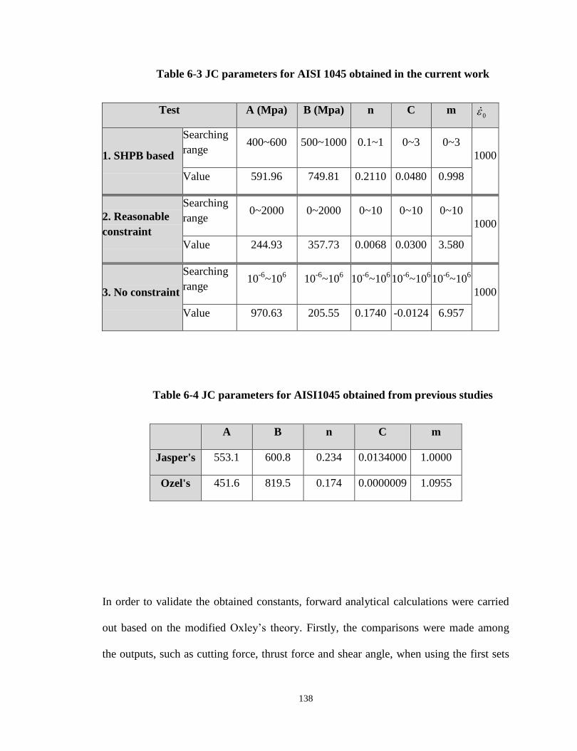
138
Table 6-3 JC parameters for AISI 1045 obtained in the current work
Test A (Mpa) B (Mpa) n C m
1. SHPB based
Searching
range 400~600 500~1000 0.1~1 0~3 0~3
1000
Value 591.96 749.81 0.2110 0.0480 0.998
2. Reasonable
constraint
Searching
range 0~2000 0~2000 0~10 0~10 0~10
1000
Value 244.93 357.73 0.0068 0.0300 3.580
3. No constraint
Searching
range 10
-6~10
6 10
-6~10
6 10
-6~10
6 10
-6~10
6 10
-6~10
6
1000
Value 970.63 205.55 0.1740 -0.0124 6.957
Table 6-4 JC parameters for AISI1045 obtained from previous studies
A B n C m
Jasper's 553.1 600.8 0.234 0.0134000 1.0000
Ozel's 451.6 819.5 0.174 0.0000009 1.0955
In order to validate the obtained constants, forward analytical calculations were carried
out based on the modified Oxley‟s theory. Firstly, the comparisons were made among
the outputs, such as cutting force, thrust force and shear angle, when using the first sets
0

139
of JC parameters in Table 6-3 and the ones from Table 6-4, since they are all based on
SHPB test. The experimental data used in this stage was the one used for the system
identification. As shown in Figure 6-5 and Figure 6-6, the new identified constants give
the best results in terms of shear angle. The cutting force and thrust force results are very
close among using three different sets of Johnson-Cook parameters and the effectiveness
of the developed methodology can basically be verified.
Figure 6-5 Comparison of shear angle with the data used for system
identification
0
5
10
15
20
25
30
35
1 2 3 4 5 6 7 8
Sh
ear
An
gle
(d
egre
e)
Test Number
experimental Ozel's Jasper's GA (SHPB based)

140
(a) Cutting force
(b) Thrust force
Figure 6-6 Comparison of cutting forces with data used for system
identification
0
500
1000
1500
2000
2500
3000
3500
4000
4500
5000
1 2 3 4 5 6 7 8
Cu
ttin
g F
orc
e (N
)
Test Number
experimental Ozel's Jasper's GA
0
500
1000
1500
2000
2500
3000
1 2 3 4 5 6 7 8
Th
rust
Fo
rce
(N)
Test Number
experimental Ozel's Jasper's GA

141
Furthermore, the experimental work done by Ivester et al [39] is utilized to verify the
developed method under various cutting conditions as shown in Table 5-1. The cutting
force predictions were carried out by using all the three sets of JC parameters obtained
from different searching schemes. The comparison was made between our results and the
duplicated results from [49], in which the PSZ is assumed equi-distant and JC parameters
are adopted from [48].
As can be seen in Figure 6-7 , most cutting forces and thrust forces calculated based on
non-equidistance PSZ analysis and newly obtained JC parameters fall into the
boundaries, except for the Test 2 and Test 6 which are relatively far below the lower
bound. The reason can be attributed to the fact that the cutting tool was assumed to be
sharp in the theoretical calculation and therefore the size effect was not taken into
account. However, the feed rates for these two tests are small and the acute rake angles
intensify the size effect. The predictions based on equidistant PSZ [49] greatly
underestimate the thrust forces. The underestimation of thrust forces is a long-lasting
problem during machining process simulations, either in analytical or numerical
simulations that material properties are obtained from SHPB tests. Based on the non-
equidistance PSZ analysis, the thrust force predictions using JC parameters obtained
from all three searching schemes showed improved results. It is also interesting to note
that the best results were achieved by using JC parameters obtained from “No constraint”
searching scheme. However, the physical significance of the five constants cannot be
maintained (see test 3 in Table 6-3), especially for „C‟ that is supposed to stand for the

142
strain rate hardening effect and now seems to become a „strain rate softening‟ factor. On
the other hand, among all three sets of JC parameters, „SHPB based‟ parameters, which
strictly preserve the physical significance, result in the worst prediction results during the
analytical simulation. This observation may suggest that the material deformation
behavior strongly depends on the combination (simultaneous variation) of the strain
hardening, strain rate hardening and thermal softening effects during metal cutting. Each
JC parameter alone or partial combination of several parameters cannot present any of
these effects. Since the condition of simultaneous variation of strain, strain rate and
temperature can hardly be achieved in any of the existing laboratory tests, it may not be
proper to take SHPB data as the reference to calibrate JC parameters for machining.

143
(a) Cutting force
(b) Thrust force
Figure 6-7 Comparison of the cutting forces using GA determined JC
parameters with the experimental data from[39]
300
500
700
900
1100
1300
1500
0 1 2 3 4 5 6 7 8
Cu
ttin
g F
orc
e (N
)
Test Number
No constraint
SHPB based
Resonable constraint
Calculation from [49]
100
200
300
400
500
600
700
800
900
1000
1100
0 1 2 3 4 5 6 7 8
Th
rust
Fo
rce
Test Number
No constraint
SHPB based
Resonable constraint
Calculation from [49]

144
6.5 Conclusion
In this chapter, an attempt has been made to identify the parameters for Johnson-Cook
material model. A MATLAB code was developed to deal with nonlinear multivariable
optimization problems using genetic algorithm. The combination of elitism and Roulette
wheel strategy is utilized as selection scheme, so that the improvement can be achieved
for each generation. The integrated single-point and multi-point crossover operator was
proposed to diversify the binary strings. The proposed “simultaneous multipoint
mutation” operator takes advantage of MATLAB‟s “parallel computing scheme” and
greatly improves the computing efficiency. Three identification tests based on different
searching scheme were carried out. The obtained Johnson-Cook parameters, along with
the parameters obtained by other researchers, were used in the forward analytical
machining simulation to examine their effectiveness. All machining force predictions
based on the proposed non-equidistance PSZ analysis showed improved results. The JC
parameters obtained without the reference of SHPB data result in the best agreement
with experimental data, suggesting that 1) Johnson-Cook constitutive equation can
fundamentally be applied to the simulation of machining process and 2) the flow
behavior of the material during machining is quite different from that under laboratory
conditions and therefore the calibration of JC constants for machining should base on the
machining tests without considering SHPB data.

145
CHAPTER 7.
TRIBOLOGICAL ANALYSIS AT THE CHIP-TOOL
INTERFACE Equation Chapter (Next) Section 1
7.1 Introduction
Chip-tool interface friction is a critical factor in determining the quality of machining
operations. It is influenced by many factors such as the stresses exerting on the cutting
tool rake face, mechanical and thermal properties of work piece and cutting tool,
tribological conditions at the chip-tool interface etc. In turn, the frictional behavior
influences the geometry of the cutting process. Early thin shear plane chip formation
models [1, 3, 5] did not take any of these factors into consideration. Instead, the
tribological behavior was represented by Coulumb coefficient of friction a
that
experimentally determined from the measured cutting forces, as shown in Equation (7.1).
tan
tan
T Ca
C T
F F
F F
(7.1)

146
In Oxley's analysis, the tribology at the chip-tool interface was assumed to be fully
represented by the shearing in the secondary shear zone. However, experimental
observations of the chip-tool interface [6, 50] suggest that the contact condition consists
of two tribological regions along the total contact length (lc). The first region is the
sticking zone near the cutting edge in which there is no relative motion between chip and
tool due to the high normal pressure. The contact nature in this region is governed by the
pure shear and the shear flow stress is uniformly distributed. Right after the sticking zone,
the second region is the sliding zone from the end of SSZ to the boundary of the contact,
in which the elastic friction dominates due to the decreased normal pressure. The normal
and shear stress distributions were suggested being the pattern shown in Figure 7-1.
Figure 7-1 Distribution of normal and shear stress at chip-tool interface

147
Many researchers have carried out experimental investigations to explain the tribology at
the tool-chip interface. However, most of the achievements are still qualitative. The
quantitative or the analytical studies are few. In particular, the work done by Karpat and
Ozel [51] and by Ozlu et al. [52] represents the state of the art in the analytical analysis
of the machining tribology. However, in [51], the coefficient of friction was calculated
based on the analysis in the secondary deformation zone, so that the reaction of the
work-tool couples was not considered at all. In [52], a more realistic method was used to
obtain the coefficient of friction for different work-tool combinations using cutting and
non-cutting tests. However, the Merchant's simple shear angle equation which is derived
for perfectly plastic material was used for the primary shear zone analysis. Moreover, the
secondary shear zone was not analyzed. In this chapter, the stress distribution in the dual
zone chip-tool interface is analyzed and incorporated in the developed chip formation
model.
7.2 Modeling dual zone chip-tool interface
In this Chapter, the focus is on the incorporation of the more realistic dual friction zone
at the chip-tool interface into the chip formation model developed in Chapter 5. As
shown in Figure 7-2, the sticking zone is assumed to be of triangular shape, followed by
the sliding zone till the end of contact length (lc).

148
Figure 7-2 Triangular dual zone model
In the region close to the cutting edge, it is well accepted that the high normal load
makes the real contact area approach the apparent contact area and the relative motion
between the chip and the tool rake face seizes up, and the zone is called the sticking
zone. In sticking zone, the shear stress at the chip-tool interface reaches the shear flow
stress of the work material. The effective flow stress ( ), if Von Mises‟ material is
assumed, is . Thus, at the location where the sticking just occurs, i.e., the normal
pressure equals , the coefficient of friction is
0.5773
cr
k k
k
(7.2)

149
From this point towards the tool cutting edge, the normal stress increases and the shear
stress keeps constant. Thus the normal stress higher than the effective flow stress (or the
coefficient of friction is less than 0.577) is expected at any location in the sticking zone.
Accordingly, the distribution of the friction coefficient can be given by
0
( )
p
cr p
kx l
p xx
x l
(7.3)
According to the pattern of normal stress shown in Figure 7-1, the normal stress
distribution at the chip-tool interface can be expressed by the power law equation
( ) 1 0N c
c
xx x l
l
(7.4)
in which N is the maximum normal stress and x is measured from the tool tip to the end
of chip-tool contact along the rake face.
The corresponding shear stress distribution, according to the sticking-sliding
configuration, can be given as
0
c p
p c
k x lx
p x l x l
(7.5)
The normal force at the chip-tool interface can be obtained by integrating the normal
stress distribution along the chip-tool contact,

150
0
11
cl
cN N
c
wlxN wdx
l
(7.6)
Thus, the maximum normal pressure at the chip-tool interface is
1
N
c
Nwl
(7.7)
On the other hand, assuming slip line AB turns through an angle to meet the
interface at right angles[10], then
022 1 2
2
n
ABN B AB AB n
AB
C nBP k k
A B
(7.8)
The moment of the force resultant at the chip-tool interface about the tool tip B is
int
0
1
cl
N
c
xN X wxdx
l
(7.9)
Substituting Equation (7.6) into Equation (7.9) and solving for the total contact length lc,
the following expression can be obtained.
int2cl X (7.10)
substituting Equation (7.8) and Equation (7.10) into Equation (7.7), the power law
exponent can be solved as
'
int
'
int
2 N
N
wX N
N wX
(7.11)

151
Friction force at the chip-tool interface can be obtained by piecewise integration of the
shear stress distribution in the form of Equation (7.5)
0
1
c
p
p
ll
C N
cl
xF k wdx wdx
l
(7.12)
Thus,
1
11
1
p
c
c
C N
p
ll
lFk
l w
(7.13)
On the other hand, the shear flow stress can be calculated with Johnson-Cook
constitutive equation
' int intint
0
11 ln 1
3
m
n wc
m w
T Tk A B C
T T
(7.14)
in which the equivalent strain, equivalent strain rate and the chip-tool interface
temperature can be estimated as follows [48]
int
1 1
2sin3AB
(7.15)
int
2
1
3
CV
t
(7.16)

152
1
22 20.06 0.195 0.5lg
int
1
sin10
cos
T TR t R t
h h
w sz
FT T T
St w
(7.17)
The length of sticking zone can be obtained from the geometry of the secondary shear
zone
2
sinp
tl
(7.18)
On the other hand, to accommodate the fact that the plastic contact ends at the location
where the sticking zone length can also be determined by satisfying
the equality
'
1
31
C
p
N
c
k
l
l
(7.19)
Noting that is the equivalent flow stress ,
can be solved as
1
' 1 Cp c
N
l l
(7.20)

153
It has been found by the authors and the work as in [53] that cutting force is not sensitive
to after using Johnson-Cook equation. In this study, Oxley's methodology is modified
as follows:
Assuming various C0
The shear angle should be the one that makes kc kc
Giving other parameters, both Equation. (7.18) and Eq. (7.20) are the functions of
, so the final can be obtained by making lp lp .
C0 is chosen based on the minimum energy principle.
The flow chart is shown in Figure 7-3.

154
Figure 7-3 Flow chart of dual friction zone chip formation model

155
7.3 Results and discussion
From the methodology described above, the cutting forces can be determined as long as
the Johnson-cook parameters are determined. The five Johnson-cook parameters for AISI
1045 used in this study is obtained using the inverse analysis: A=591.96 MPa; B=749.81
Mpa; n=0.2108; C=0.0048; m=0.998. The coefficient of friction is set 0 6.
Force data from the experimental work in [39] is used to verify the developed method.
The comparisons of cutting forces and thrust forces are shown in Figure 7-4.
It can be seen that the overall cutting forces and thrust forces are slightly overestimated.
It has been believed that the coefficient of friction on the sliding zone varies with tool-
work couples. In this study, the coefficient of friction is set as 0.6. However, different
will definitely influence the machining forces and other processing parameters.
Furthermore, different Johnson-Cook constants will also influence the predicted results.

156
(a) Cutting force
(b) Thrust force
Figure 7-4 Comparison of cutting forces predicted by dual zone friction
model
300
500
700
900
1100
1300
1500
0 1 2 3 4 5 6 7 8
Cu
ttin
g F
orc
e (N
)
Test Number
experimental
upper bound experimental
lower bound Prediction
100
200
300
400
500
600
700
800
900
1000
1100
0 1 2 3 4 5 6 7 8
Th
rust
Fo
rce
Test Number
experimental
upper bound experimental
lower bound Prediction

157
7.4 Conclusion
In this chapter, frictional behavior at the chip-tool interface is analyzed based on the dual
friction zone hypothesis. A triangular secondary shear zone is assumed. According to
Von Mise's flow rule, 0.577 is chosen as the critical coefficient of friction to define the
boundary of sticking and sliding zones.. With the input of sliding coefficient of friction,
a new methodology is proposed to carry out the cutting force simulation. In comparison
of previous models, the new model is closer to the physics of metal cutting and able to
provide more information, such as stress distributions on the tool rake face, the length of
sticking and sliding zone, etc. The accurate determination of sliding friction coefficient
under the conditions of metal cutting would lead to the improved model and profound
analysis in the effect of cutting conditions on these processing parameters.

158
CHAPTER 8.
THESIS SUMMARY AND FUTURE WORK
8.1 Thesis summary
In the current work, the focus is on the investigation of mechanics and the development
of analytical chip formation model during metal cutting. Oxley's predictive machining
theory [10], in which material properties are the major input for the model development,
is selected as the groundwork that the current research is based on.
Oxley's model was firstly extended to allowing for the application to various engineering
materials and the simulation of end milling process. The model was further modified to
consider the velocity field across the primary shear zone, leading to a more
phenomenological description of the continuous deformation during chip formation. An
inverse analysis methodology that combines the newly developed chip formation model
and optimization algorithm was then developed to determine the flow stress data of the

159
material under the conditions of metal cutting. Taking advantage of the global searching
nature of genetic algorithm, three tests were carried out based on different searching
schemes. Without setting any constraint on searching range, the obtained results was
found surpassing all other searching schemes in which the physical significance of each
parameter of interest is more or less retained. This result led to the conclusion that SHPB
data obtained under laboratory conditions may not be the proper reference to calibrate
material properties for machining. Lastly, the tribological analysis was carried at the
chip-tool interface, along with the newly proposed methodology for the determination of
various processing parameters.
The effort made in this dissertation is primarily for the establishment of a generalized
algorithm by which the better presentation of the material deformation, the determination
of material flow properties and the prediction of processing parameters of interest can be
systematically integrated.
8.2 Future work
The velocity field in the secondary deformation zone can be further analyzed, so
that the variation of the chip flow velocity on the tool rake face, shear strain and
strain rate along and across the secondary shear zone can be investigated.

160
Inverse analysis can be applied to chip-tool interface, in an attempt to identify
tribological characteristics as a function of cutting conditions and material
properties.

161
REFERENCES
1 Piispanen, V. Theory of formation of metal chips. Journal of Applied Physics,
1948, 19(10), 876-881.
2 Merchant, M.E. Mechanics of the metal cutting process. I. Orthogonal cutting
and a type 2 chip. Journal of Applied Physics, 1945, 16(5), 267-275.
3 Merchant, M.E. Mechanics of the metal cutting process. Ii. Plasticity conditions
in orthogonal cutting. Journal of Applied Physics, 1945, 16(6), 318-324.
4 Lee, E.H. and Shaffer, B.W. Theory of plasticity applied to problem of
machining. American Society of Mechanical Engineers -- Transactions -- Journal
of Applied Mechanics, 1952, 19(2), 234-239.
5 Okushima, K. and Hitomi, K. An analysis of the mechanism of orthogonal
cutting and its application to discontinuous chip formation. Journal of
Engineering for Industry, Transactions of the ASME, 1961, 545-556.
6 Zorev, N.N. Interrelationship between shear processes occurring along tool face
and on shear plane in metal cutting. Proceedings of the International Production
Engineering Research Conference, Sep 9-12 1963, pp. 42-49 (American Society
of Mechanical Engineers (ASME), New York, NY, United States, 1963).
7 Oxley, P.L.B. A strain-hardening solution for the "shear angle" in orthogonal
metal cutting. International Journal of Mechanical Sciences, 1961, 3(1-2), 68-79.
8 Oxley, P.L.B. and Hastings, W.F. Predicting the strain rate in the zone of
intense shear in which the chip is formed in machining from the dynamic flow
stress properties of the work material and the cutting conditions. Proceedings of
the Royal Society of London. Series A, Mathematical and Physical Sciences, 1977,
356(1686), 395-410.

162
9 Oxley, R. Mechanics of orthogonal machining. Allowing for the effects of strain
rate and temperature on tool-chip friction. 1968, 183(22), 417-438.
10 Oxley, P.L.B. The mechanics of machining: An analytical approach to assessing
machinability. (Ellis Horwood, 1989).
11 Boothroyd, G. Temperatures in orthogonal metal cutting. Proceedings of the
Institution of Mechanical Engineers, 1963, 177(29), 789-810.
12 Johnson, G.J. and Cook, W.H. A constitutive model and data for metals
subjected to large strains, high strain rates and high temperatures. Proceedings of
the 7th International Symposium on Ballistics, pp. 541-5471983).
13 Martellotti, M.E. Analysis of milling process. American Society of Mechanical
Engineers -- Transactions, 1941, 63(8), 677-695.
14 Martellotti, M.E. Analysis of milling process, part ii -- down milling. American
Society of Mechanical Engineers -- Transactions, 1945, 67(4), 233-251.
15 Smith, S. and Tlusty, J. Overview of modeling and simulation of the milling
process. Journal of engineering for industry, 1991, 113(2), 169-175.
16 Wang, W.P. Solid modeling for optimizing metal removal of three-dimensional
nc end milling. Journal of Manufacturing Systems, 1988, 7(1), 57-65.
17 Koenigsberger, F. and Sabberwal, A.J.P. An investigation into the cutting
force pulsations during milling operations. International Journal of Machine Tool
Design and Research, 1961, 1(1-2), 15-33.
18 Sabberwal, A.J.P. Cutting forces in down milling. International Journal of
Machine Tool Design and Research, 1962, 2(1), 27-41.
19 Kline, W.A., DeVor, R.E. and Lindberg, J.R. The prediction of cutting forces
in end milling with application to cornering cuts. International Journal of
Machine Tool Design and Research, 1982, 22(1), 7-22.

163
20 Kline, W.A. and DeVor, R.E. The effect of runout on cutting geometry and
forces in end milling. International Journal of Machine Tool Design and
Research, 1983, 23(2-3), 123-140.
21 Sutherland, J.W. and DeVor, R.E. Improved method for cutting force and
surface error prediction in flexible end milling systems. Journal of engineering
for industry, 1986, 108(Compendex), 269-279.
22 Tlusty, J. and MacNeil, P. Dynamics of cutting forces in end milling. Annals of
the CIRP, 1975, 24(1), 21-25.
23 Sutherland, J.W. Dynamic model of the cutting force system in the end milling
process. Sensors and Controls for Manufacturing - 1988, November 27, 1988 -
December 2, 1988, pp. 53-62 (Publ by American Soc of Mechanical Engineers
(ASME), Chicago, MI, USA, 1988).
24 Armarego, E.J.A. and Deshpande, N.P. Computerized end-milling force
predictions with cutting models allowing for eccentricity and cutter deflections.
CIRP Annals - Manufacturing Technology, 1991, 40(1), 25-29.
25 Yucesan, G., Xie, Q. and Bayoumi, E. Determination of process parameters
through a mechanistic force model of milling operations. International Journal of
Machine Tools and Manufacture, 1993, 33(4), 627-641.
26 Yucesan, G. and Altintas, Y. Improved modelling of cutting force coefficients
in peripheral milling. International Journal of Machine Tools and Manufacture,
1994, 34(4), 473-487.
27 Bayoumi, A.E., Yucesan, G. and Kendall, L.A. Analytic mechanistic cutting
force model for milling operations: A case study of helical milling operation.
Journal of engineering for industry, 1994, 116(3), 331-339.
28 Liang, S.Y. and Wang, J.J.J. Milling force convolution modeling for
identification of cutter axis offset. International Journal of Machine Tools and
Manufacture, 1994, 34(8), 1177-1190.
29 Wang, J.J.J., Liang, S.Y. and Book, W.J. Convolution analysis of milling force
pulsation. Journal of engineering for industry, 1994, 116(1), 17-25.

164
30 Junz Wang, J.J. and Liang, S.Y. Chip load kinematics in milling with radial
cutter runout. Journal of engineering for industry, 1996, 118(1), 111-116.
31 Stabler, G.V. Fundamental geometry of cutting tools. Institution of Mechanical
Engineers -- Proceedings, 1951, 165(63), 14-21.
32 Hu, R.S., Mathew, P., Oxley, P.L.B. and Young, H.T. Allowing for end cutting
edge effects in predicting forces in bar turning with oblique machining conditions.
Proceedings of the Institution of Mechanical Engineers. Part C. Mechanical
engineering science, 1986, 200(C2), 89-99.
33 Young, H.-T., Mathew, P. and Oxley, P.L.B. Predicting cutting forces in face
milling. International Journal of Machine Tools and Manufacture, 1994, 34(6),
771-783.
34 Yalcin, C. A flexible-tool mechanistic milling force model. (University of New
Hampshire, 2003).
35 Tounsi, N., Vincenti, J., Otho, A. and Elbestawi, M.A. From the basic
mechanics of orthogonal metal cutting toward the identification of the
constitutive equation. International Journal of Machine Tools and Manufacture,
2002, 42(12), 1373-1383.
36 Dudzinski, D. and Molinari, A. A modelling of cutting for viscoplastic
materials. International Journal of Mechanical Sciences, 1997, 39(4), 369-389.
37 Astakhov, V.P., Osman, M.O.M. and Hayajneh, M.T. Re-evaluation of the
basic mechanics of orthogonal metal cutting: Velocity diagram, virtual work
equation and upper-bound theorem. International Journal of Machine Tools and
Manufacture, 2001, 41(3), 393-418.
38 Moufki, A., Molinari, A. and Dudzinski, D. Modelling of orthogonal cutting
with a temperature dependent friction law. Journal of the Mechanics and Physics
of Solids, 1998, 46(10), 2103-2138.
39 Ivester, R.W., Kennedy, M., Davies, M., Stevenson, R., Thiele, J., Furness, R.
and Athavale, S. Assessment of machining models: Progress report. Machining
Science and Technology: An International Journal, 2000, 4(3), 511 - 538.

165
40 Pujana, J., Arrazola, P.J., M'Saoubi, R. and Chandrasekaran, H. Analysis of
the inverse identification of constitutive equations applied in orthogonal cutting
process. International Journal of Machine Tools and Manufacture, 2007,
47(Compendex), 2153-2161.
41 Shatla, M., Kerk, C. and Altan, T. Process modeling in machining. Part i:
Determination of flow stress data. International Journal of Machine Tools and
Manufacture, 2001, 41(10), 1511-1534.
42 Sartkulvanich, P., Koppka, F. and Altan, T. Determination of flow stress for
metal cutting simulation--a progress report. Journal of Materials Processing
Technology, 2004, 146(1), 61-71.
43 Chandrasekaran, H., M'Saoubi, R. and Chazal, H. Modelling of material flow
stress in chip formation process from orthogonal milling and split hopkinson bar
tests. Machining Science and Technology, 2005, 9(Compendex), 131-145.
44 Lei, S., Shin, Y.C. and Incropera, F.P. Material constitutive modeling under
high strain rates and temperatures through orthogonal machining tests. Journal of
Manufacturing Science and Engineering, 1999, 121(4), 577-585.
45 Ozel, T. and Zeren, E. A methodology to determine work material flow stress
and tool-chip interfacial friction properties by using analysis of machining.
Journal of Manufacturing Science and Engineering, 2006, 128(1), 119-129.
46 Holland, J.H. Adaption in natural and artificial systems. (The MIT Press, 1992).
47 Hillier, F.S. and Lieberman, G.J. Introduction to operation research, 8th
edition. (McGraw Hill, 2005).
48 Jaspers, S. and Dautzenberg, J.H. Material behaviour in conditions similar to
metal cutting: Flow stress in the primary shear zone. Journal of Materials
Processing Technology, 2002, 122(2-3), 322-330.
49 Lalwani, D.I., Mehta, N.K. and Jain, P.K. Extension of oxley's predictive
machining theory for johnson and cook flow stress model. Journal of Materials
Processing Technology, 2009, 209(12-13), 5305-5312.

166
50 Childs, T.H.C., Mahdi, M.I. and Barrow, G. On the stress distribution between
the chip and tool during metal turning. CIRP Annals - Manufacturing Technology,
1989, 38(1), 55-58.
51 Karpat, Y. and Ozel, T. Predictive analytical and thermal modeling of
orthogonal cutting process---part i: Predictions of tool forces, stresses, and
temperature distributions. Journal of Manufacturing Science and Engineering,
2006, 128(2), 435-444.
52 Ozlu, E., Budak, E. and Molinari, A. Analytical and experimental investigation
of rake contact and friction behavior in metal cutting. International Journal of
Machine Tools and Manufacture, 2009, 49(11), 865-875.
53 Adibi-Sedeh, A.H., Madhavan, V. and Bahr, B. Extension of oxley's analysis
of machining to use different material models. Journal of Manufacturing Science
and Engineering, 2003, 125(4), 656-666.