analytical evaluation of the accuracy of … 2.8. force-creep curves for various rail and wheel...

ANALYTICAL EVALUATION OF THE ACCURACY OF ROLLER RIG

DATA FOR STUDYING CREEPAGE IN RAIL VEHICLES

Alexander Keylin

Thesis submitted to the faculty of Virginia Polytechnic Institute and State

University in partial fulfillment of the requirements for the degree of

MASTER OF SCIENCE

In

Mechanical Engineering

Mehdi Ahmadian, Committee Chair

Corina Sandu

Saeid Taheri

December 3, 2012

Blacksburg, VA

Keywords: roller rigs, wheel-rail contact, friction modeling, normal contact,

tangent contact, rolling contact.

ANALYTICAL EVALUATION OF THE ACCURACY OF ROLLER RIG DATA FOR STUDYING

CREEPAGE IN RAIL VEHICLES

Alexander Keylin

ABSTRACT

The primary purpose of this research is to investigate the effectiveness of a scaled roller rig for

accurately assessing the contact mechanics and dynamics between a profiled steel wheel and rail, as is

commonly used in rail vehicles. The established creep models of Kalker and Johnson and Vermeulen are

used to establish correction factors, scaling factors, and transformation factors that allow us to relate the

results from a scaled rig to those of a tangent track. Correction factors, which are defined as the ratios of

a given quantity (such as creep coefficient) between a roller rig and a track, are derived and used to relate

the results between a full-size rig and a full-size track. Scaling factors are derived to relate the same

quantities between roller rigs of different scales. Finally, transformation factors are derived by combining

scaling factors with correction factors in order to relate the results from a scaled roller rig to a full-size

tangent track. Close-end formulae for creep force correction, scaling, and transformation factors are

provided in the thesis, along with their full derivation and an explanation of their limitations; these

formulae can be used to calculate the correction factors for any wheel-rail geometry and scaling.

For Kalker’s theory, it is shown that the correction factor for creep coefficients is strictly a function of

wheel and rail geometry, primarily the wheel and roller diameter ratio. For Johnson and Vermeulen’s

theory, the effects of creepage, scale, and load on the creep force correction factor are demonstrated. It is

shown that INRETS’ scaling strategy causes the normalized creep curve to be identical for both a full-size

and a scaled roller rig. It is also shown that the creep force correction factors for Johnson and

Vermeulen’s model increase linearly with creepage, starting with the values predicted by Kalker’s theory.

Therefore, Kalker’s theory provides a conservative estimate for creep force correction factors. A case

study is presented to demonstrate the creep curves, as well as the correction and transformation factors,

for a typical wheel-rail configuration. Additionally, two studies by other authors that calculate the

correction factor for Kalker’s creep coefficients for specific wheel-rail geometries are reviewed and show

full agreement with the results that are predicted by the formulae derived in this study. Based on a review

of existing and past roller rigs, as well as the findings of this thesis, a number of recommendations are

given for the design of a roller rig for the purpose of assessing the wheel-rail contact mechanics. A

scaling strategy (INRETS’) is suggested, and equations for power consumption of a roller rig are derived.

Recommendations for sensors and actuators necessary for such a rig are also given. Special attention is

given to the resolution and accuracy of velocity sensors, which are required to properly measure and plot

the creep curves.

iii

Acknowledgements

First of all, I would like to thank the Federal Railroad Administration and our program manager, Mr.

Ali Tajaddini, for providing the funding for the project of which this thesis is a part. Without their support,

this research would not have been possible.

I would like to thank my coauthors – Dr. Mehdi Ahmadian, Mr. Ali Tajaddini, and Mr. Mehdi Taheri –

on the conference paper which became the foundation for this thesis.

I would like to thank my research advisor and committee chair, Dr. Mehdi Ahmadian, for giving me

the opportunity to conduct this research, for providing guidance, and for being extremely supportive and

understanding when my classes, volunteer work, and other life circumstances interfered with my research

duties. Special thanks are also due to the members of my committee, Professors Corina Sandu and Saeid

Taheri.

I am grateful to the personnel of the Blacksburg Fire Department for being equally understanding and

for helping me balance my studies with my duties to the department.

I am thankful to the faculty of the University of Pittsburgh, most notably Dr. Daniel Cole, Dr. Mark

Kimber, Dr. Ian Nettleship, and Dr. Jeffrey Vipperman, for encouraging me to pursue a graduate degree.

Last, but not least, I am extremely grateful to my parents, Vladimir and Svetlana Keylin, without

whom I would not have been able to accomplish anything I have achieved. Thank you for everything.

iv

Contents

1 Introduction ........................................................................................................................................... 1

1.1 Motivation ..................................................................................................................................... 1

1.2 Problem Statement ........................................................................................................................ 2

1.3 Research Approach and Main Contribution .................................................................................. 2

1.4 Dissertation Outline ...................................................................................................................... 3

2 Literature Survey ................................................................................................................................... 4

2.1 Approach ....................................................................................................................................... 4

2.2 Normal Contact Problem .............................................................................................................. 4

2.3 Tangent Contact Problem .............................................................................................................. 6

2.4 Roller Rigs .................................................................................................................................. 13

3 Development of Key Relations ............................................................................................................ 16

3.1 The Normal Contact Problem ..................................................................................................... 16

3.1.1 The Formulation ...................................................................................................................... 16

3.1.2 Surface Curvatures and Radii ................................................................................................. 17

3.2 General Remarks on Creepages and Creep Forces ..................................................................... 20

3.2.1 The Definition of Creepages ................................................................................................... 20

3.2.2 The Relationships between Creepages and Creep Forces ....................................................... 22

3.3 Specific Creepage Theories......................................................................................................... 24

3.3.1 Kalker’s Linear Theory ........................................................................................................... 24

3.3.2 Johnson and Vermeulen’s Theory ........................................................................................... 25

4 Comparison Methodology ................................................................................................................... 27

4.1 General Remarks ......................................................................................................................... 27

4.2 Creepage Variation ...................................................................................................................... 27

4.3 Scaling......................................................................................................................................... 28

4.3.1 Normal Contact Problem ........................................................................................................ 28



4.4 Roller Rig vs. Track Correction Factors ..................................................................................... 33

4.4.1 Normal Contact ....................................................................................................................... 33



4.5 Transformation Factors ............................................................................................................... 38


v


4.6 Influence of Specific Scaling Strategies ..................................................................................... 40

4.6.1 General Remarks ..................................................................................................................... 40

4.6.2 MMU’s Strategy ...................................................................................................................... 41

4.6.3 DLR’s Strategy ........................................................................................................................ 44

4.6.4 INRETS’ Strategy ................................................................................................................... 46

5 Case Study ........................................................................................................................................... 48

5.1 Case Study Data .......................................................................................................................... 48

5.2 Kalker’s Linear Theory ............................................................................................................... 48

5.3 Johnson and Vermeulen’s Theory ............................................................................................... 54

5.4 Results of Other Studies .............................................................................................................. 59

5.5 Key Findings ............................................................................................................................... 59

6 Roller Rig Design Considerations ....................................................................................................... 60

6.1 General Considerations ............................................................................................................... 60

6.2 Scaling......................................................................................................................................... 64

6.3 Sensors ........................................................................................................................................ 64

6.4 Actuators and Constraints ........................................................................................................... 66

6.5 Power Consumption .................................................................................................................... 67

6.5.1 General Considerations ........................................................................................................... 67

6.5.2 Jaschinski’s (DLR) Scaling Strategy with Density SF of 1 .................................................... 67

6.5.3 Jaschinski’s Strategy with a Non-unity Density SF ................................................................ 68

6.5.4 Pascal’s (INRETS) Scaling Strategy ....................................................................................... 68

6.5.5 Iwnicki’s (MMU) Scaling Strategy ......................................................................................... 69

6.5.6 Modified Power Equations ...................................................................................................... 69

6.6 Data Processing ........................................................................................................................... 71

7 Summary and Conclusions .................................................................................................................. 72

7.1 Summary ..................................................................................................................................... 72

7.2 Conclusions ................................................................................................................................. 72

7.3 Future Work ................................................................................................................................ 73

8 References ........................................................................................................................................... 74

vi

List of Figures

Figure 2.1. Redtenbacher’s model for normal contact. ................................................................................. 5

Figure 2.2. True shape of wheel-rail contact patch as a function of contact point location. ......................... 6

Figure 2.3. Wheel/rail contact patch according to Boedecker. ...................................................................... 7

Figure 2.4. Tangential stress distribution (solid line) according to Carter. ................................................... 8

Figure 2.5. Kalker’s FASTSIM algorithm, adapted from [2] ........................................................................ 9

Figure 2.6. Dependency of force-creep curve slope onto surface roughness, adapted from [4] ................. 10

Figure 2.7. A decrease in creep force at large creepages............................................................................. 11

Figure 2.8. Force-creep curves for various rail and wheel surface conditions. ........................................... 11

Figure 2.9. Slope and maximum of force-creep curve under the conditions of wet vs. dry friction. .......... 12

Figure 3.1. Hertzian contact problem, adapted from[16]. ........................................................................... 16

Figure 3.2. Contact patch shape for various wheel locations with respect to the rail. ................................ 18

Figure 3.3. Example of a variation of the wheel and rail’s transverse radii. All dimensions are in mm. .... 18

Figure 3.4. Velocities of wheel and rail/roller at the point of contact, adapted from [2] ............................ 21

Figure 3.5. Creepage curve according to Coulomb’s model. ...................................................................... 22

Figure 3.6. Creepage curve according to Kalker’s linear model, adjusted for saturation. .......................... 23

Figure 3.7. A “generic” creepage curve according to the nonlinear theories. ............................................. 23

Figure 5.1. Correction factor for creep forces per unit creepage as a function of a roller’s rolling radius

(r21): full-size and 1/5-scale roller rigs, adapted from [1] ........................................................................... 48

Figure 5.2. TF for creep forces per unit creepage as a function of a roller radius: full-size and 1/5-scale

roller rigs, adapted from [1] ........................................................................................................................ 49

Figure 5.3. Transformation factor for creep forces per unit creepage as a function of length SF, adapted

from [1] ....................................................................................................................................................... 50

Figure 5.4. Correction factor for creep forces per unit creepage as a function of wheel and roller radii

ratio: full-size and 1/5-scale roller rigs, adapted from [1] .......................................................................... 51

Figure 5.5. Transformation factor for creep forces per unit creepage as a function of wheel and roller radii

ratio: full-size and 1/5-scale roller rigs, adapted from [1] .......................................................................... 51

Figure 5.6. CF and TF for creep forces per unit creepage as a function of length SF with roller radius

fixed, adapted from [1] ............................................................................................................................... 52

Figure 5.7. CF for creep forces per unit creepage as a function of roller radius; load scaling factor is equal

to the r11/r21 ratio; full-size and 1/5-scale rigs, adapted from [1] ................................................................ 53

Figure 5.8. TF for creep forces per unit creepage as a function of roller radius; load scaling factor is equal

to the r11/r21 ratio; full-size and 1/5-scale rigs, adapted from [1].............................................................. 53

Figure 5.9. Normalized creep curves and creep force correction factors for a full-size track and roller rig.

.................................................................................................................................................................... 54

vii

Figure 5.10. Correction factors for longitudinal and lateral creep forces as functions of creepages. Dashed

lines represent non-linear relationship, solid lines represent adjusted linear approximation; dotted-dashed

(-.-.) lines represent the difference between linear and non-linear functions (right-hand vertical scale);

base roller rig configuration ........................................................................................................................ 56


lines represent non-linear relationship; solid lines represent adjusted linear approximation; dotted-dashed


load per wheel is 170 kN ............................................................................................................................ 56


lines represent non-linear relationship; solid lines represent adjusted linear approximation; dotted-dashed


roller radius is 2m, other parameters are as in base configuration. ............................................................. 57

Figure 5.13. Creep curves and creep force correction factors for a 1/5-scale roller rig scaled according to

INRETS’ strategy (𝑓𝑙 = 5, 𝑓𝑤 = 25). ...................................................................................................... 58

Figure 6.1. Vertical plane roller. (Source: [89]) .......................................................................................... 61

Figure 6.2. Internal vertical plane roller. (Source: [89]) ............................................................................. 61

Figure 6.3. Horizontal roller rig. (Source: [89]) ......................................................................................... 61

Figure 6.4. Short-stroke oscillating rail. (Source: [89]) .............................................................................. 62

Figure 6.5. High-speed shooting rail. (Source: [89]) .................................................................................. 62

Figure 6.6. Modified roller rig. (Source: [89]) ............................................................................................ 63

List of Tables

Table 1: Roller rig concepts with top scores. (Source: [89]) ....................................................................... 63

Table 2. Anticipated sensor requirements for a roller rig. (Source: [89]) ................................................... 65

viii

Nomenclature

Wheel and rail geometry:

𝑟0: rolling radius of the wheel

𝑟11: rolling radius of the wheel (adjusted for conicity)

𝑟12: transverse radius of the wheel

𝑟21: rolling radius of the roller

𝑟22: transverse radius of the roller

𝛾: wheel conicity angle

Normal contact:

𝑎, 𝑏: Hertzian contact ellipse radii

𝐴, 𝐵: contact surfaces curvature parameters

𝑔𝑎𝑏: contact patch radii ratio (a/b)

𝑒: contact patch geometry parameter

𝑚,𝑛: Hertzian contact ellipse parameters

𝑁: vertical load per wheel (adjusted for conicity)

𝑄: vertical load per wheel (unadjusted)

Tangent contact:

𝑐11, 𝑐22, 𝑐23: Kalker’s linear creepage coefficients (longitudinal, lateral-yaw, and lateral-spin)

𝑓11, 𝑓22, 𝑓23: Kalker’s creep forces per unit creepage

𝐹: total creep force

𝐹𝑥: longitudinal creep force

𝐹𝑦: lateral creep force

𝜇: friction coefficient

𝜈𝑥: longitudinal creepage

𝜈𝑦: lateral creepage

𝜈𝑥,𝑠𝑎𝑡: longitudinal saturation creepage

𝜈𝑦,𝑠𝑎𝑡: lateral saturation creepage

𝜏: reduced total creepage

𝜏𝑥: reduced longitudinal creepage

𝜏𝑦: reduced lateral creepage

ix

𝜏𝑥,𝑠𝑎𝑡: reduced longitudinal saturation creepage

𝜏𝑦,𝑠𝑎𝑡: reduced lateral saturation creepage

𝜑: spin creepage

Material properties:

𝐸: Young’s modulus

𝐺: shear modulus

𝜈: Poisson’s ratio

𝜌: density

Correction factors (CF):

𝑐𝑎𝑏: CF for 𝑎𝑏

𝑐𝑏𝑎: CF for 𝑏

𝑎

𝑐𝐴𝐵: correction factor for 𝐴

𝐵

𝑐𝐴+𝐵: CF for (𝐴 + 𝐵)

𝑐𝑐11, 𝑐𝑐22, 𝑐𝑐23: CF for Kalker’s linear creepage coefficients

𝑐𝑓11, 𝑐𝑓22, 𝑐𝑓23: CF for creep forces per unit creepage

𝑐𝐹: CF for total creep force

𝑐𝐹𝑥: CF for longitudinal creep force

𝑐𝐹𝑦: CF for lateral creep force

𝑐𝜏: CF for reduced creepage

𝑐𝜏𝑥: CF for reduced longitudinal creepage

𝑐𝜏𝑦: CF for reduced lateral creepage

𝑐𝜏𝑥,𝑠𝑎𝑡: CF for reduced longitudinal saturation creepage

𝑐𝜏𝑦,𝑠𝑎𝑦: CF for reduced lateral saturation creepage

Scaling factors (SF):

𝑓𝑎: acceleration SF

𝑓𝑎𝑏: SF for 𝑎𝑏

𝑓𝑏𝑎: SF for 𝑏

𝑎

𝑓𝐴𝐵: SF for 𝐴

𝐵

x

𝑓𝐴+𝐵: SF for (𝐴 + 𝐵)

𝑓𝑐: damping SF

𝑓𝑐𝑇: torsion damping SF

𝑓𝐸: Young’s modulus SF

𝑓𝐹: creep force SF

𝑓𝐹𝑜𝑟𝑐𝑒: force (unspecified) SF

𝑓𝐹𝑥: longitudinal creep force SF

𝑓𝐹𝑦: lateral creep force SF

𝑓𝑘: stiffness SF

𝑓𝑘𝑇: torsion stiffness SF

𝑓𝑘𝑥: elastic force SF

𝑓𝑙: length SF

𝑓𝑚𝑎: inertial forces SF

𝑓𝑚𝑔: gravity force SF

𝑓𝑃𝑅: Poisson’s ratio SF

𝑓𝑡: time SF

𝑓𝑇: torque SF

𝑓𝑉: velocity SF

𝑓𝑤: wheel load/normal force SF

𝑓𝜌: density SF

𝑓𝜎: stress SF

𝑓𝜏𝑥,𝑠𝑎𝑡: SF for reduced longitudinal saturation creepage

𝑓𝜏𝑦,𝑠𝑎𝑦: SF for reduced lateral saturation creepage

Transformation factors (TF):

𝑇𝑓11, 𝑇𝑓22, 𝑇𝑓23: TF for creep forces per unit creepage

𝑇𝐹: TF for total creep force

𝑇𝐹𝑥: longitudinal creep force TF

𝑇𝐹𝑦: lateral creep force TF

𝑇𝜏𝑥,𝑠𝑎𝑡: TF for reduced longitudinal saturation creepage

𝑇𝜏𝑦,𝑠𝑎𝑦: TF for reduced lateral saturation creepage

1

1 Introduction

1.1 Motivation

The term “roller rig,” as it is used here, describes a testing fixture that is being used to evaluate

locomotives, railcars, and their components. A roller rig normally consists of one or more rollers, i.e.,

wheels that have their tread shaped like the crown of a rail. A piece of rolling stock that is being tested is

placed onto the roller, and either the roller, the axle of the rolling stock, or both are actuated while the

tested piece is constrained in the longitudinal direction. This method of testing allows examination of the

behavior of the rolling stock on a track without actually placing it onto the track. This method has a

number of advantages:

1. Construction and maintenance of railroad track specifically for the purpose of testing the

rolling stock is expensive, and typically a roller rig is a more affordable alternative; use of an

existing track for testing can also be expensive due to the inability to use the track for

commercial purposes while it is being used for testing.

2. Using a roller rig gives a researcher more control over experimental conditions. Parameters

such as gauge, alignment, rail cant, rail profile, rail surface roughness and its condition (dry,

wet, oily, etc.) can be relatively easily controlled on a roller rig, but not on a track.

3. Experiments on a roller rig can be more data-rich, because it is easier to instrument a roller

than a track of substantial length. Furthermore, rollers, unlike rails, can easily be actuated, i.e.

force and excitation can be applied to them to study the response of the tested rolling stock.

4. Tests that would be too expensive or impossible to conduct on a track due to safety reasons

can easily be conducted on a roller rig (e.g., conditions of near-derailment).

Because of these advantages, roller rigs have been extensively used since the early 20th century and

are still used today. Examples of research conducted on roller rigs include, but are not limited to:

1. Investigation of longitudinal and lateral dynamics of wheelsets, bogies (trucks), and car

bodies.

2. Investigation and experimental validation of wheel-rail contact theories.

3. Investigation of wheel and rail wear and damage.

4. Testing of rolling stock suspension elements.

5. Testing of traction motors and brakes.

6. Evaluation of friction modifiers and other measures directed at reducing railroad operating

expenses and increasing the safety of operation.

2

Nevertheless, the advantages of roller rigs come at a cost. Due to differences in geometry, wheel-

roller contact is inherently different from wheel-rail contact. Dynamic behavior of rolling stock is also

affected by the need to constrain the longitudinal motion of the rolling stock relative to the rollers.

Additional difficulties are presented by scaling a roller rig. These differences must be carefully accounted

for such that the researcher can correctly extrapolate the behavior of rolling stock onto a test stand onto its

behavior on an actual track.

This thesis was written as part of a larger research project that evaluates the feasibility of constructing

a roller rig whose main purpose would be the evaluation of existing wheel-rail contact theories, and also

gives recommendations on its implementation (actuators, sensors, scaling, etc.)

1.2 Problem Statement

The first goal of this work is to clearly describe the difference between wheel-rail and wheel-roller

creepage behavior. Although this has been done in other studies that we will describe below, these studies

tend to describe the difference for specific testing configurations, while we are attempting to present

clearly-derived, preferably closed-end formulae that can be used for any given wheel and rail/roller

profiles, loads, scaling factors and scaling strategies.

The second goal is to provide recommendations on the design of a roller rig. Rather than

recommending a specific design, we analyze the existing roller rigs and try to provide researchers with

guidelines to help them design a roller rig with a specific purpose in mind. The pros and cons of different

design solutions are discussed.

1.3 Research Approach and Main Contribution

The task of describing the difference between creep curves in cases of wheel-rail and wheel-roller

contact is divided into three stages.

First, we examine the difference in creepage behavior arising from rail/roller geometry for a full-size

rail vehicle. We then explore the influence of scaling the vehicle and the rail/roller onto the creepage

behavior, and finally, we combine the results.

We will use two creepage theories: Kalker’s linear theory and Johnson and Vermeulen’s theory. Both

will be described in detail later. Kalker’s theory was chosen because it is very widely used, gives closed-

end relationships, and is relatively easy to work with. As such, it has become the de facto creepage model

over the years; furthermore, it serves as a foundation for later and more sophisticated theories. Johnson

and Vermeulen’s theory was chosen because it is non-linear (i.e. accounts for contact patch saturation)

3

while still giving closed-end relationships; this theory has been widely acclaimed and experimentally

verified.

1.4 Dissertation Outline

Chapter 2 discusses the wheel-rail creepage phenomenon and the history of its research from the 19th

century to present years, as well as the history of roller rigs. We begin with the normal (vertical) contact

between wheel and rail, continue with tangent contact, and end with an overview of various creepage

theories and various roller rigs that were used historically and/or that are still in use or being developed

today.

In Chapter 3, we give a detailed discussion of both Kalker’s and Johnson and Vermeulen’s theories,

which will serve as a basis for our analysis in the next chapter.

In Chapter 4, we derive the correction and transformation factors between tangent track and roller rigs

of various scales and scaling strategies, starting with a difference in normal contact and concluding with

the discussion of specific scaling strategies.

In Chapter 5, we present a case study to illustrate the relationships we obtained in Chapter 4. We also

compare our findings to those of other authors and briefly discuss the differences.

In Chapter 6, we state our considerations regarding the design of a roller rig.

Finally, Chapter 7 presents a summary of findings and recommendations for future work.

Portions of this thesis (primarily Chapters 4 and 5) are based on the paper produced by the author and

his coauthors for the ASME 2012 Rail Transportation Division Fall Technical Conference [1].

4

2 Literature Survey

2.1 Approach

The search of the relevant literature is conducted using a number of review articles [2-8]. The works

cited in each of the review articles are examined, and then the sources cited in these works are examined.

The Google Scholar search engine was used to locate more recent works that referenced the examined

sources. Additional searches were conducted in Google Scholar using keywords such as “roller rig,”

“wheel-rail contact,” “creepage,” “Kalker’s coefficients,” etc.

2.2 Normal Contact Problem

The problem of finding the traction forces can be broken down into two parts:

1. Finding the dimensions and shape of the contact patch, as well as the normal pressure distribution

in it (i.e. the normal contact problem).

2. Finding the relationship between creepages and tangential forces (a.k.a. creep forces) based on

the shape of the patch (i.e., the tangent contact problem).

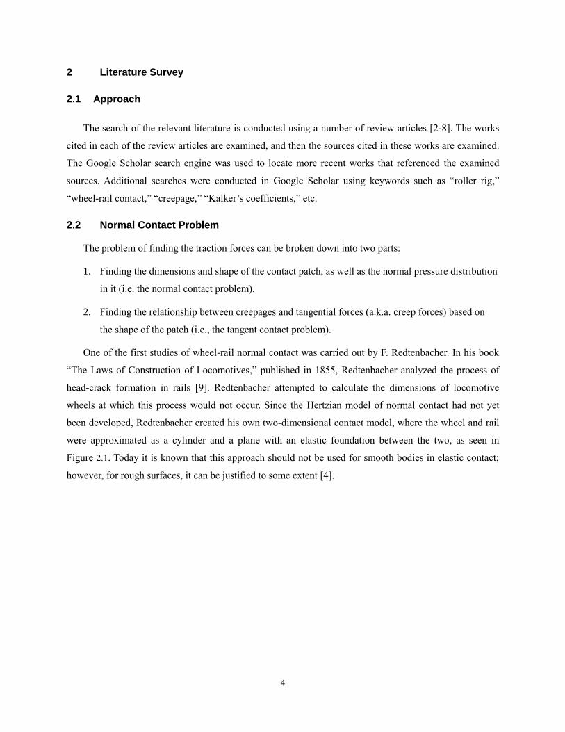
One of the first studies of wheel-rail normal contact was carried out by F. Redtenbacher. In his book

“The Laws of Construction of Locomotives,” published in 1855, Redtenbacher analyzed the process of

head-crack formation in rails [9]. Redtenbacher attempted to calculate the dimensions of locomotive

wheels at which this process would not occur. Since the Hertzian model of normal contact had not yet

been developed, Redtenbacher created his own two-dimensional contact model, where the wheel and rail

were approximated as a cylinder and a plane with an elastic foundation between the two, as seen in

Figure 2.1. Today it is known that this approach should not be used for smooth bodies in elastic contact;

however, for rough surfaces, it can be justified to some extent [4].

5

Figure 2.1. Redtenbacher’s model for normal contact.

(Source: Redtenbacher’s work, adapted from [4])

Nearly 30 years later, Hertz published two influential works on contact mechanics, which described

the distribution of normal force and the dimensions of contact patch between contact surfaces [10, 11].

Although Hertzian theory rests on a number of rather restrictive assumptions, it is still widely used in

studying wheel-rail contact mechanics and dynamics, and serves as a foundation for many tangent contact

theories, both empirical and analytical [2, 4, 12]. We will discuss Hertzian theory in detail later in this

paper.

Nevertheless, the dimensions of contact patch given by Hertzian theory are often a poor

representation of the true contact shape, as indicated in Figure 2.2, primarily due to non-constant surface

curvatures [4, 13, 14]. For this reason, a number of non-Hertzian and semi-Hertzian normal contact

theories have been used to describe wheel-rail normal contact [2, 15-24]. Some of these theories are

modifications of Hertzian theory, and some are based on different principles. These theories tend to be

computationally intensive, allowing their use in some wheel-rail software, but preventing establishing

simple, close-form relationships, as intended in this study.

6

Figure 2.2. True shape of wheel-rail contact patch as a function of contact point location.

(Source: Piotrowski’s work, adapted from [4])

2.3 Tangent Contact Problem

The most simplistic way to solve the tangent contact problem is by assuming that the wheel and the

rail are perfectly rigid bodies, and applying Coulomb’s law. In this case, the traction or braking force will

be a function of normal force and Coulomb’s friction coefficient. This approach can be useful for certain

7

kinds of dynamics problems, but is of little use if one is trying to solve problems dealing with wheel and

rail wear, traction losses, etc., thereby necessitating the development of rolling contact theories [12].

A number of authors cite Carter’s 1916 work [25] as the first study of longitudinal rail-wheel contact

[2, 7, 12]. Nearly 30 years before Carter, Boedecker published a paper on stability of a rigid two-axle

bogie, in which he presented what was possibly the first study of tangent wheel-rail contact [26].

Boedecker assumed a circular contact patch and applied localized Coulomb’s friction law, yielding a

simple but fully non-linear model, as shown in Figure 2.3 [4]. This model has not become widely used.

Figure 2.3. Wheel/rail contact patch according to Boedecker.

(Source: Boedecker’s work, adapted from [4])

Similarly to Boedecker, Carter was studying the stability of a rigid bogie, but his model of tangent

contact was very different. In his 1916 publication, Carter described the concept of creepage (relative

motion between the surfaces in rolling contact) and stated that traction or braking force (aka creep force)

is proportional to the creepage. Carter did not derive or explain this assumption, nor did he derive the

proportionality constant. It is possible that Carter was influenced by Reynolds’ work; in 1874, Reynolds

introduced the concept of creepage between belts and pulleys, and noted that such a concept could apply

to rolling wheels as well [7, 27].

In 1926, Carter published an article in which he quantified the linear relationship between creepage

and creep force [28]. In this paper, he treated wheel-rail contact as a two-dimensional problem of contact

between a cylinder and a plane. Based on Love’s derivation of normal stresses and strains in an elastic

medium, Carter described the distribution of tangential stresses in the contact zone, as shown in Figure 2.4

[29]. Furthermore, he described the saturation of the creep force with increasing creepage and predicted

frictional losses in a locomotive driving wheel [7, 12, 28].

8

Figure 2.4. Tangential stress distribution (solid line) according to Carter.

(Source: Carter’s work, adapted from [4])

Fromm, also in 1926, solved a similar problem in a different way [30]. Although he shared some

assumptions with Carter, he analyzed the contact between two cylinders, rather than between a cylinder

and a plane. Due to the complexity of the solution, only numerical solutions could be obtained [4].

Carter’s work was not recognized immediately, but later gained acceptance and eventually was widely

used until the 1960s [2, 4]. In 1950, Poritsky published results similar to Carter’s [7, 31].

In 1958, Johnson derived an approximate three-dimensional solution to the rolling contact problem,

considering both longitudinal and lateral creep forces [32]. Johnson analyzed an elastic sphere rolling on

an elastic plane and assumed that the overall contact patch is circular, and that the adhesion region is also

circular and is tangent to the leading edge of the contact patch, as shown in 1938 by Cattaneo [7, 33, 34].

Johnson verified his findings experimentally and also investigated the effects of spin creepage on lateral

creep force [7, 35].

In 1963, Haines and Ollerton expanded Carter’s theory onto a more general case where a contact

patch is elliptical (although they only described longitudinal creepage) [36]. They separated the elliptical

contact patch into longitudinal strips and assumed that Carter’s longitudinal shear stress distribution

applied to each strip [7, 36]. This allowed them to clarify the shape of the adhesion area (which they

described as “lemon-shaped”) within the contact patch. Meanwhile, Vermeulen and Johnson expanded on

Johnson’s earlier work and obtained an approximate solution for creep forces in the case of an elliptical

contact patch, neglecting the spin creepage [7, 32, 34]. Vermeulen and Johnson’s findings, along with

Kalker’s, are discussed in more detail later in this paper.

During the 1960s, De Pater and Kalker had developed a complete analytical solution to wheel-rail

contact theory; their solution is now referred to as linear theory [7, 12]. De Pater started with the

9

simplified case (circular contact patch and zero Poisson ratio), and Kalker expanded his findings to a

more general case of an elliptical contact with a non-zero Poisson ratio [2, 12, 37, 38]. This resulted in the

introduction of Kalker’s famous coefficients, which describe the linear relationship between creepage and

creep forces in longitudinal and lateral directions. Although De Pater and Kalker’s solution was, in a

sense, more complete than those of other authors, it was only applicable to low creepages at which slip

area in a contact patch is much less than adhesion area. In other words, Kalker’s linear theory does not

account for saturation.

Although Vermeulen and Johnson’s original work was done before Kalker had introduced his

coefficients, the relationships found by them are now commonly stated in terms of Kalker’s coefficients,

thanks to the work of Shen, Hendrick and Elkins [39]. This work combines Kalker’s accuracy at low

creepages with Vermeulen and Johnson’s ability to describe saturation.

More recently, several empirical methods to describe the creep curve have been developed [2], such

as Kalker’s empirical proposition, as well as Ohyama’s and CHOPAYA’s (Ayasse–Chollet–Pascal)

exponential saturation law [13, 40]. These methods present closed-form force-creep models (neglecting

the spin creep); however, they are still somewhat inferior to Johnson and Vermeulen’s model in terms of

simplicity and ease of computation.

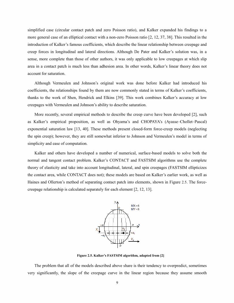
Kalker and others have developed a number of numerical, surface-based models to solve both the

normal and tangent contact problem. Kalker’s CONTACT and FASTSIM algorithms use the complete

theory of elasticity and take into account longitudinal, lateral, and spin creepages (FASTSIM ellipticizes

the contact area, while CONTACT does not); these models are based on Kalker’s earlier work, as well as

Haines and Ollerton’s method of separating contact patch into elements, shown in Figure 2.5. The force-

creepage relationship is calculated separately for each element [2, 12, 13].

Figure 2.5. Kalker’s FASTSIM algorithm, adapted from [2]

The problem that all of the models described above share is their tendency to overpredict, sometimes

very significantly, the slope of the creepage curve in the linear region because they assume smooth

10

contact surfaces and fail to account for the roughness of the real wheels and rails, as seen in Figure 2.6 [4,

41].

Figure 2.6. Dependency of force-creep curve slope onto surface roughness, adapted from [4]

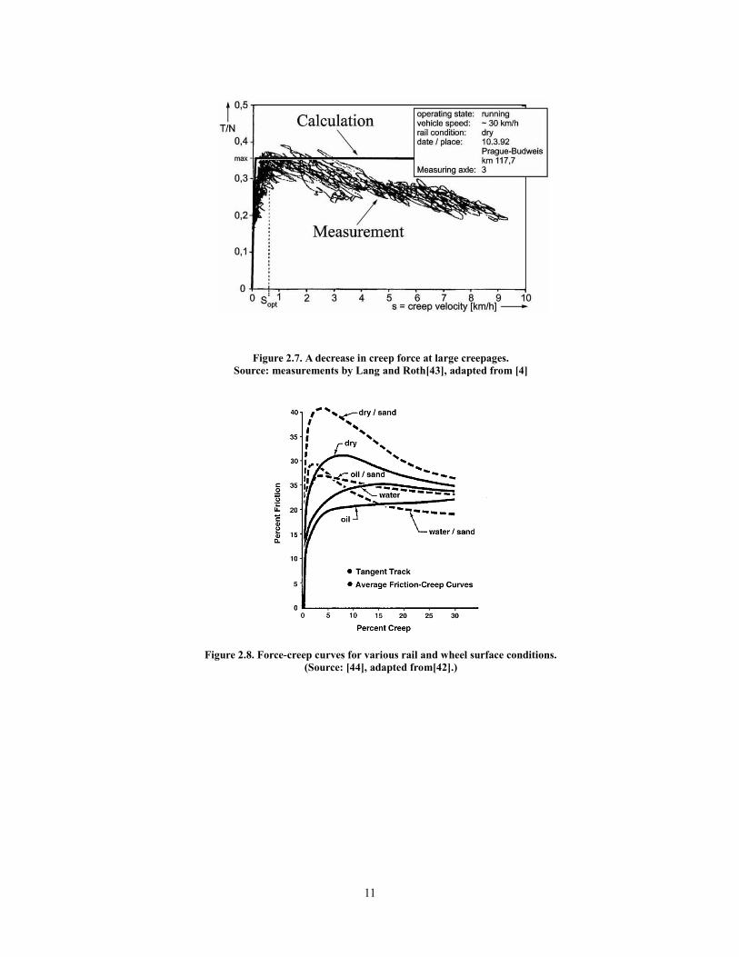
The behavior of creep force past the saturation point presents an additional challenge. The theories

discussed so far predict a constant creep force as the creepage increases past the saturation point.

However, it is known from experiments that creep force reaches a maximum and then decreases with the

increase in creepage, as shown in Figure 2.7, presumably due to an increase in temperature of surfaces at

the point of contact [4]. Furthermore, the shape of the creep curve varies significantly with surface

condition, as seen in Figure 2.8 and Figure 2.9 [42].

11

Figure 2.7. A decrease in creep force at large creepages.

Source: measurements by Lang and Roth[43], adapted from [4]

Figure 2.8. Force-creep curves for various rail and wheel surface conditions.

(Source: [44], adapted from[42].)

12

Figure 2.9. Slope and maximum of force-creep curve under the conditions of wet vs. dry friction.

(Source: [45])

These discrepancies have recently been investigated by multiple scholars [4, 42, 45-47]. Empirical

expressions have been proposed that describe friction coefficient as a function of creep velocity; in

addition, correction factors for Kalker’s coefficients as a function of rail surface condition have been

measured and published [45].

Recently, several studies have proposed the use of beam and bristle adhesion models (normally used

for modeling automobile tires) to describe the wheel-rail force-creepage relationship in order to develop a

control system for wheel slip [48, 49]. The authors claim a good fit between theoretical and experimental

data for a wide range of conditions.

A simplified empirical model was recently developed by Malvezzi et al. for the purpose of

constructing a scaled roller rig [50, 51]. The model describes the adhesion peak and decrease at high

creepages, which are discussed above.

Matsumoto et al. introduced the “thin film lubrication theory” and “boundary lubrication theory” into

FASTSIM in order to predict creep characteristics in the presence of a friction modifier [52].

A model of wheel-rail tangential contact under the conditions of degraded adhesion (i.e. in the

presence of contaminants between the two surfaces) has recently been proposed by Pugi et al. [53]. The

authors point out that at very high creepages, the coefficient of friction may actually increase due to the

destruction of contaminant and polishing of the contact surfaces.

13

2.4 Roller Rigs

Zhang et al., as well as Jaschinski et al., provide an excellent overview of the history of roller rigs

from the early 1900s up to the early 2000s [3, 5].

In 1904, one of the first roller rigs was built at the Swindon Works in Britain. It was a full-size rig that

was designed to study the performance of steam locomotives, specifically, their pulling power at different

speeds [54].

In the 1920s, Carter used a scaled tangent track rig to conduct experiments in rail vehicle dynamics

[3]. In the 1930s, model tests were conducted on a roller rig in Japan by Musashi, although not much

information about it is available. One-tenth- and one-fifth-scale roller rigs were used at The Railway

Technical Research Institute in Japan during the 1950s to support design efforts for rail vehicle

suspension [55]. In 1957, a full-scale, two-axle roller rig was constructed at RTRI and was used for more

than 30 years. The rig used an eccentric roller to create sinusoidal excitation and was utilized to study

hunting, derailment, regenerative braking and various aspects of dynamics of new types of bogies, in part

to support the development of Shinkansen high-speed trains [56]. The rig was upgraded in 1989 to

increase its maximum speed to 500 km/h, and to supplement each roller with actuators for lateral, vertical,

and roll vibration.

In the 1950s, the C&O – B&O railroad in the United States conducted multiple tests on a one-tenth

scale roller rig to facilitate the development of new passenger and freight railcars [3].

In 1963-1964, British Railways constructed a number of roller rigs, both scaled and full-size, to

conduct a number of studies of vehicle dynamics. An additional four-axle roller rig was built in 1969, but

it did not see much use because a more advanced test track was completed [57] .

In 1979-1982, Sweet et al. at Princeton University performed investigations concerning the

mechanics of derailment using a fifth-scale model of a freight bogie. Forces in the model were carefully

scaled according to similarity laws [58, 59].

In the 1970s, various studies were done on a scaled roller rig at RWTH Aachen in Germany [60].

During the same decade, the roller rig of the Deutsche Bahn AG was constructed in Munich. This is a

full-size, four-axle roller rig capable of achieving speeds of up to 500 km/h and allowing the simulation of

various track irregularities using hydraulic actuators. The rig has been used to verify various theoretical

models as well as to conduct commercial tests. Jaschinski gives a thorough description of the rig’s design

and of various studies conducted on it, such as investigations of creepage, vibration, ride comfort and

stability, failure tests, testing of active systems, etc. [61-64].

14

In 1978, a full-size, four-axle roller rig (auxiliary support stands were available to accommodate six-

or eight-axle locomotives and railcars) called the Roll Dynamics Unit (RDU) in Pueblo, Colorado became

operational [65]. The unit was equipped with hydraulic actuators to apply forces to a bogie side frame, a

sophisticated data acquisition system, and flywheels for simulation of inertia associated with braking and

acceleration. RDU was used to test locomotive traction motors, as well as to study general vehicle-track

dynamics. The researchers who operated that rig, which has since been decommissioned, noted that test

setup was very useful in studying rail vehicle lateral dynamics, but using it to study creep forces proved

problematic [66].

In the 1980s, a number of scaled roller rigs were used at DLR in Oberpfaffenhofen [67-69]. One of

these rigs, a one-fifth-scale, two-axle setup, was used to develop the software package SIMPACK; this rig

is thoroughly described by Jaschinski et al.

A unique roller rig operated from 1984 until 1992 at INRETS in Grenoble, France. This unit consisted

of a 13-m diameter roller, which could be driven at speeds up to 250 km/h. Combined with a test bogie of

¼ scale, this rig allowed the researchers to obtain wheel-rail contact conditions very similar to those seen

on a tangent track [70]. Numerous experiments were performed on it, most of them dealing with hunting

stability and with measuring Kalker’s coefficients [71]. The results were used to develop the simulation

software VOCO.

In 1992, a roller rig at the Rail Technology Unit of the Manchester Metropolitan University became

operational [72, 73].

Jaschinski et al. and Zhang et al. briefly describe additional roller rigs, such as a full-size rig in

Chengdu, nearly identical to the rig in Munich, and a full-size Curved Track Simulator in Ottawa (the

latter has since been dismantled).

Some of the most recently constructed roller rigs include the two roller rigs (a full-scale, two-axle rig

and its scaled copy) at the Research Centre of Firenze Osmannoro, Italy [51, 74]. The rigs simulate

degraded adhesion conditions to test rail vehicle response; rather than physically introducing a

contaminant at the interface, its presence is being simulated by controlling the angular speeds of the

rollers.

A full-scale, one-axle roller rig is being used by Voestalpine Schienen GmbH in Linz, Austria [75].

This rig utilizes a short (1.5-m) piece of rail, rather than a roller, and is being used to investigate rail wear

and rolling contact fatigue. Consequently, the speed of the wheel is limited to 0.5 m/s.

A one-tenth-scale, two-axle roller rig has been used by Matsumoto et al. in Japan [52] to investigate

creepage under various surface conditions, especially in the presence of a friction modifier. Small

15

creepages can be accurately produced by controlling the differential gear and measuring torque in real

time.

A one-fourth-scale roller rig with a single 1070-mm roller, known as JD-1, exists at the Tribology

Research Institute in Chengdu, China. It has been used to study rail corrugation in particular, and rail-

wheel adhesion behavior in general [76, 77].

A one-tenth-scale track exists at the Chiba Experimental Station, IIS, The University of Tokyo. The

track’s total length is 25m, and it features tangent sections, as well as transition curve and constant curve

sections. It has been successfully used to test scale models of bogies [78, 79].

Korea Railroad Research Institute uses a one-fifth-scale, two-axle roller rig and a one-fifth-scale, 27-

m track to test bogies as well as entire rail vehicles. The track consists of two tangent sections and a curve

[80, 81].

Scaling strategies used in some of the rigs described above (DLR rig, INRETS rig, and MMU rig) are

described later in this thesis.

16

3 Development of Key Relations

3.1 The Normal Contact Problem

3.1.1 The Formulation

The traditional method used to solve the first problem is via Hertzian contact theory. We will follow

the process as outlined by Ayasse and Chollet [2].

Hertzian theory is based on a number of key assumptions [2, 4]:

1. The kinematic equations and the materials elastic properties are linear.

2. Wheel and rail material exhibit completely elastic behavior (no plastic deformation).

3. Wheel and rail material is homogeneous and its properties are isotropic.

4. The contact surfaces are perfectly smooth and there is no friction between them.

5. Contact surfaces curvature is constant within the contact patch.

6. Contact surfaces radii of curvature are much larger than the dimensions of the contact patch.

We treat wheel and rail as elastic bodies 1 and 2; each of the two bodies has a longitudinal (rolling)

radius ri1 and a transverse radius ri2, where i is the index of the body (1 or 2).

Specifically, as shown in Figure 3.1, r11 is an effective rolling radius of the wheel (defined later), r12 is

the transverse radius of the wheel (in a purely conical wheel, it is considered infinite), r21 is the rolling

radius of the rail or roller (infinite in a case of tangent track, and finite in a case of roller), and r22 is the

crown radius of the rail or roller.

Figure 3.1. Hertzian contact problem, adapted from[16].

17

3.1.2 Surface Curvatures and Radii

There are multiple formulations to the Hertzian problem. In this particular case, Ayasse and Chollet

define the variables A and B that describe the longitudinal and transverse curvature of the two bodies at

the point of contact.

𝐴 =1

2(

1

𝑟11+

1

𝑟21) 3.1

𝐵 =1

2(

1

𝑟12+

1

𝑟22) 3.2

Note, however, that r11 is not the actual rolling radius of the wheel, but is an effective rolling radius.

Ayasse and Chollet define it in terms of an actual rolling radius r0 and wheel conicity 𝛾 at the point of

contact:

1

𝑟11=

cos 𝛾

𝑟0 3.3

Solving Eq. 3.3 for r11 we obtain:

𝑟11 =𝑟0

cos 𝛾 3.4

For typical values of wheel conicity (between 0 and 5 degrees), the difference between r11 and r0 is

<0.5% , so this correction may not be necessary and we can assume that r11 is the rolling radius of the

wheel. Similarly, the angle of attack (yaw angle) of the wheel, 𝛼𝑦𝑎𝑤, is in the same range, so correcting

the radii or curvature for this angle seems unnecessary and is not reported in the literature.

According to Hertzian formulation, the contact patch will have the shape of an ellipse. Assuming that

the wheel and rail are made of the same material, the contact ellipse radii’s exact values can be

determined via:

𝑎 = 𝑚(3𝑁(1 − 𝜈2)

2𝐸(𝐴 + 𝐵))

13

3.5

𝑏 = 𝑛 (3𝑁(1 − 𝜈2)

2𝐸(𝐴 + 𝐵))

13

3.6

In this case, a is the longitudinal radius (along the direction of rolling), and b is the transverse radius,

as shown for various wheel positions in Figure 3.2.

18

Figure 3.2. Contact patch shape for various wheel locations with respect to the rail.

(Source: [12])

The magnitudes of the radii will vary depending on the location of the wheel-rail contact point due to

the fact that the wheel and the rail’s transverse curvatures are non-constant, as seen in Figure 3.3.

Figure 3.3. Example of a variation of the wheel and rail’s transverse radii. All dimensions are in mm.

(Source: Piotrowski’s work, adapted from [4])

The Hertzian coefficients m and n can be determined by calculating elliptical integrals or by

interpolating from tables [12, 82]:

𝑚 = (2𝑔2𝐄(𝑒)

𝜋)

13

3.7

𝑛 = (2𝐄(𝑒)

𝜋𝑔𝑎𝑏)

13

3.8

Where:

𝑔𝑎𝑏 =𝑎

𝑏 3.9

19

𝑒 = (1 −1

𝑔𝑎𝑏2 ) 3.10

and E(e) is the complete elliptical integral of the second kind.

In order to obtain an easy-to-manipulate, closed-form solution, we will use an analytical

approximation:

𝑏

𝑎=

𝑛

𝑚≈ (

𝐴

𝐵)0.63

3.11

(𝑚𝑛)32 ≈

(

1 +

𝐴𝐵

2√𝐴𝐵 )

0.63

3.12

Ayasse and Chollet note that when A/B is close to 1, the exponent would be 2/3 rather than 0.63.

However, 0.63 is a better approximation for slender ellipses, and it gives an error of no more than 5% for

b/a between 1/25 and 25.

Solving Eq. 3.11 for n:

𝑛 = 𝑚(𝐴

𝐵)0.63

3.13

Similarly, solving 3.12 for n:

𝑛 =1

𝑚

(

1 +

𝐴𝐵

2√𝐴𝐵 )

0.42

3.14

Combining 3.13 and 3.14 we obtain:

𝑚(𝐴

𝐵)0.63

=1

𝑚

(

1 +

𝐴𝐵

2√𝐴𝐵 )

0.42

3.15

We then solve 3.15 for m:

𝑚 = √

(

1 +

𝐴𝐵

2√𝐴𝐵 )

0.42

(𝐴

𝐵)−0.63

= (𝐴

𝐵)−0.315

(

1 +

𝐴𝐵

2√𝐴𝐵 )

0.21

3.16

20

Combining 3.13 and 3.16, we have

𝑛 = (𝐴

𝐵)0.315

(

1 +

𝐴𝐵

2√𝐴𝐵 )

0.21

3.17

Knowing Hertzian coefficients m and n, we can obtain contact ellipse radii a and b via Eqs. 3.5

and 3.6.

Note that normal load N in Eqs. 3.5 and 3.6 can be adjusted for wheel conicity at the point of contact:

𝑁 = 𝑄 cos 𝛾 3.18

However, this influence is very minor (for the wheel conicity of 5 degrees, cos 𝛾 = 0.996195) and

can be safely neglected in most applications, just like the correction in Eq. 3.4.

The main limitations of Hertzian contact theory are the assumption of one-point contact, the

assumption that ellipse radii are much smaller than the contact surfaces’ radii of curvature, and the

assumption that these curvatures are constant in the vicinity of the contact point. While these assumptions

are reasonable in the case of a tread contact on an unworn wheel, they become problematic in the case of

flange contact, as well as in severely worn wheels and rails, where multipoint or conformal contact may

occur.

3.2 General Remarks on Creepages and Creep Forces

3.2.1 The Definition of Creepages

In order for creep forces to appear, there must be a small apparent slip between the wheel and the rail

surface. If this slip is normalized against the wheel and rail’s absolute velocities, it is called creepage. We

will use the definitions of creepages that are given by Ayasse and Chollet and illustrated in Figure 3.4 [2].

21

Figure 3.4. Velocities of wheel and rail/roller at the point of contact, adapted from [2]

If we take V0 and V1 to be the absolute linear velocities of the wheel and rail/roller at the point of

contact, and Ω0 and Ω1 to be, respectively, their angular velocities, we can define the creepages in terms

of these velocities’ projections onto the x-axis (longitudinal), y-axis (lateral), and z-axis (vertical), as

shown in Figure 3.4:

𝜈𝑥 =proj(𝑥)(𝑉0

− 𝑉1 )

12 (𝑉0

+ 𝑉1 )

3.19

𝜈𝑦 =proj(𝑦)(𝑉0

− 𝑉1 )

12 (𝑉0

+ 𝑉1 )

3.20

𝜑 =proj(𝑧)(Ω0

− Ω1 )

12 (𝑉0

+ 𝑉1 )

3.21

Note that longitudinal and lateral creepages are dimensionless quantities, while rotation, or spin

creepage, has dimensions of m-1

. We will discuss the implications of this fact later.

Also note that creepage is not always normalized against the average velocity of the wheel and rail, as

described here; a number of authors normalize it against the train speed with respect to a static frame of

22

reference. This difference is of little significance at low creepages, but can be substantial at high

creepages [83].

Although longitudinal, lateral, and spin creepages depend on the speeds of the wheel and rail, they do

not influence each other, i.e., a change in longitudinal creepage will not cause a change in lateral

creepage, and vice versa. Furthermore, according to creep theories that are discussed here, creepages do

not influence the shape of the contact patch, its size, or the normal pressure distribution within it.

3.2.2 The Relationships between Creepages and Creep Forces

All of the theories discussed below state that the creep forces and moments are functions of these

creepages. In other words, creep forces depend not on absolute or relative velocities of the wheel and rail

per se, but on these relative velocities normalized against their absolute velocities.

The two extremes are Coulomb’s model and Kalker’s linear model.

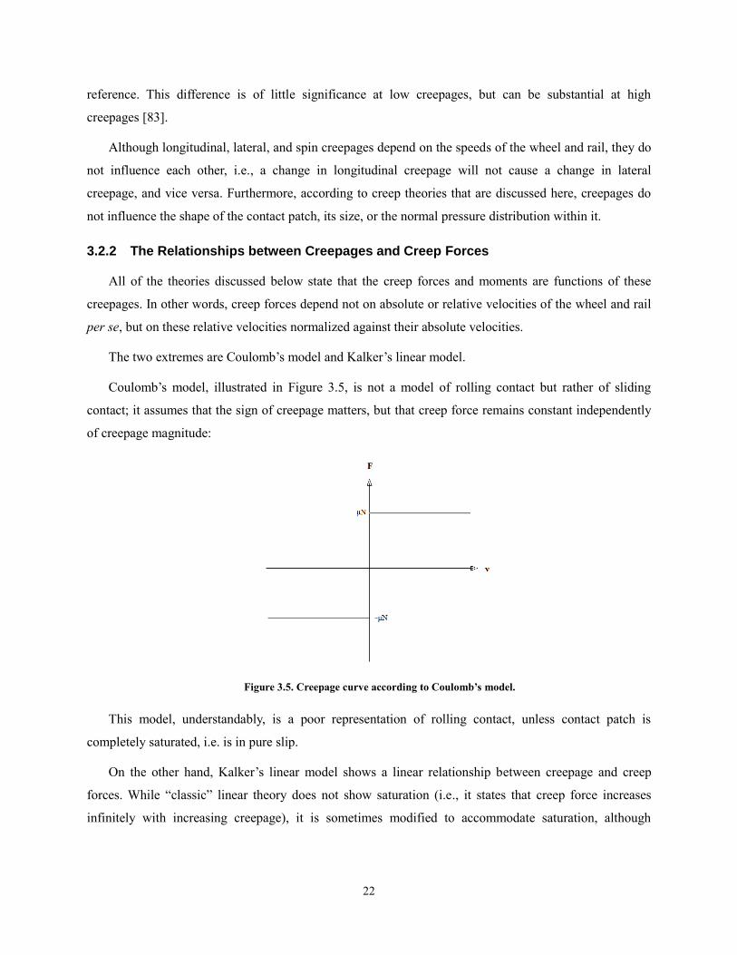
Coulomb’s model, illustrated in Figure 3.5, is not a model of rolling contact but rather of sliding

contact; it assumes that the sign of creepage matters, but that creep force remains constant independently

of creepage magnitude:

Figure 3.5. Creepage curve according to Coulomb’s model.

This model, understandably, is a poor representation of rolling contact, unless contact patch is

completely saturated, i.e. is in pure slip.

On the other hand, Kalker’s linear model shows a linear relationship between creepage and creep

forces. While “classic” linear theory does not show saturation (i.e., it states that creep force increases

infinitely with increasing creepage), it is sometimes modified to accommodate saturation, although

23

somewhat crudely (see, for instance, “Kalker’s linear theory with saturation” option in the multibody

simulation software package SIMPACK), as seen in Figure 3.6.

Figure 3.6. Creepage curve according to Kalker’s linear model, adjusted for saturation.

Non-linear models fall, in terms of creepage curve, somewhere between these two extremes; at very

low creepages they behave similarly to Kalker’s linear model, then they gradually approach saturation, as

shown in Figure 3.7.

Figure 3.7. A “generic” creepage curve according to the nonlinear theories.

(Source: [24])

We will now discuss some of these theories more closely.

24

3.3 Specific Creepage Theories

3.3.1 Kalker’s Linear Theory

The definitions of slip and creepage given in Eqs. 6.26 to 3.21 treat the wheel and rail as rigid bodies.

In reality, both bodies deform near the point of contact, and the points in the contact patch are being

displaced from their original locations. The part of the contact patch where the rate of displacement

“cancels” the apparent slip becomes the adhesion area; the rest of the patch is in slip, i.e. there is not only

apparent rigid-body slip, but also true slip of surfaces past each other [84]. Kalker’s linear theory assumes

that for small creepages, slip area is negligibly small compared to the adhesion area. Under this

assumption, and also assuming Hertzian normal force distribution, Kalker derives the tangential stresses

at various points throughout the adhesion area. By integrating these stresses over the area of the contact

patch, Kalker obtains the total creep forces per unit creepage (essentially, the slope of the creepage curve

in Figure 3.6).

The dependency between creepage and creep forces and moments can be expressed in a matrix form

[84]:

[

𝐹𝑥𝐹𝑦𝑀𝑧

] = −𝐺𝑎𝑏 [

𝑐11 0 0

0 𝑐22 √𝑎𝑏𝑐23

0 −√𝑎𝑏 𝑐33

] [

𝜈𝑥

𝜈𝑦

𝜑] 3.22

The quantities c11, c22, c23, and c33 are referred to as Kalker’s creepage coefficients; typically, tables

are used to calculate them from dimensions of the contact patch and the materials’ Poisson ratio.

Alternatively, Ayasse and Chollet list the following polynomial approximations for some of these

coefficients; these are valid for a steel wheel and rail, providing the b/a ratio is within the interval 1/25 to

25 [2]:

𝑐11 = 3.2893 +

0.975

𝑏𝑎

−0.012

(𝑏𝑎)

2 3.23

𝑐22 = 2.4014 +

1.3179

𝑏𝑎

−0.02

(𝑏𝑎)

2 3.24

𝑐23 = 0.4147 +

1.0184

𝑏𝑎

+0.0565

(𝑏𝑎)

2 −0.0013

(𝑏𝑎)

3 3.25

Since these coefficients are functions of b/a, it will be useful to obtain this ratio from Eqs. 3.1, 3.2,

and 3.11:

25

𝑏

𝑎=

𝑛

𝑚= (

𝐴

𝐵)0.63

= (

1𝑟11

+1𝑟21

1𝑟12

+1𝑟22

)

0.63

3.26

Often in literature on this subject, the authors are concerned primarily with longitudinal and lateral

creep forces Fx and Fy, essentially ignoring the moment Mz [2, 85]. In such cases, the relationship shown

in Eq. 6.26 will be described next.

For longitudinal traction force:

𝐹𝑥 = 𝑓11𝜈𝑥 3.27

For lateral force:

𝐹𝑦 = 𝑓22𝜈𝑦 + 𝑓23𝜑 3.28

Where f11, f22, and f23 are Kalker’s creep forces per unit creepage, defined as follows:

𝑓11 = −𝐺𝑎𝑏𝑐11 3.29

𝑓22 = −𝐺𝑎𝑏𝑐22 3.30

𝑓23 = 𝐺𝑎𝑏√𝑎𝑏𝑐23 3.31

As mentioned earlier, longitudinal and lateral creepages are non-dimensional, while spin creepage, by

default, has dimensions of m-1

. If we normalized the spin creepages by √𝑎𝑏, then Eq. 3.31 would not have

the term √𝑎𝑏 in it.

3.3.2 Johnson and Vermeulen’s Theory

Vermeulen and Johnson’s theory is an approximate one: it operates on longitudinal and lateral

creepages only, ignoring the spin creepage [2, 85]. It introduces the notion of reduced longitudinal and

lateral creepages:

𝜏𝑥 =𝐺𝑎𝑏𝑐11𝜈𝑥

3𝜇𝑁 3.32

𝜏𝑦 =𝐺𝑎𝑏𝑐22𝜈𝑦

3𝜇𝑁 3.33

The total reduced creepage coefficient is a function of longitudinal and lateral creepages:

26

𝜏 = √𝜏𝑥2 + 𝜏𝑦

2 = √(𝐺𝑎𝑏𝑐11𝜈𝑥

3𝜇𝑁)2

+ (𝐺𝑎𝑏𝑐22𝜈𝑦

3𝜇𝑁)

2

=𝐺𝑎𝑏

3𝜇𝑁√𝑐11

2 𝜈𝑥2 + 𝑐22

2 𝜈𝑦2

3.34

When the total reduced creepage coefficient reaches 1, contact patch is fully saturated, i.e. is in 100%

slip. Past this point, friction force is described by the Coulomb law:

𝐹

𝜇𝑁= 1, 𝜏 > 1 3.35

Before the saturation, friction force is described by:

𝐹

𝜇𝑁= 1 − (1 − 𝜏)3 = 1 − (1 −

𝐺𝑎𝑏

3𝜇𝑁√𝑐11

2 𝜈𝑥2 + 𝑐22

2 𝜈𝑦2)

3

,

0 < 𝜏 < 1

3.36

For pure longitudinal creepage:

𝐹

𝜇𝑁= 1 − (1 − 𝜏)3 = 1 − (1 −

𝐺𝑎𝑏𝑐11𝜈𝑥

3𝜇𝑁)3

, 0 < 𝜏 < 1 3.37

For pure lateral creepage:

𝐹

𝜇𝑁= 1 − (1 − 𝜏)3 = 1 − (1 −

𝐺𝑎𝑏𝑐22𝜈𝑦

3𝜇𝑁)

3

, 0 < 𝜏 < 1 3.38

Now we can find the saturation point (i.e. creepage at which saturation occurs) in pure longitudinal

creepage:

𝜏𝑠𝑎𝑡 = 𝜏𝑥,𝑠𝑎𝑡 =𝐺𝑎𝑏𝑐11𝜈𝑥,𝑠𝑎𝑡

3𝜇𝑁= 1 3.39

Solving for 𝜈𝑥,𝑠𝑎𝑡 yields:

𝜈𝑥,𝑠𝑎𝑡 =3𝜇𝑁

𝐺𝑎𝑏𝑐11 3.40

Similarly, the saturation point in pure lateral creepage is:

𝜈𝑦,𝑠𝑎𝑡 =3𝜇𝑁

𝐺𝑎𝑏𝑐22 3.41

27

4 Comparison Methodology

4.1 General Remarks

In order to quantify the relationship between different wheel-rail configurations, we define the

concepts of scaling factor, correction factor, and transformation factor.

Scaling factor (SF) is a term commonly used in literature on roller rigs. It refers to the ratio of a

certain quality (length, velocity, mass, etc.) between full-size and scaled models. For instance, a creep

force scaling factor of 5 means that creep forces in the model are 1/5 of the corresponding forces in a full-

size model.

Correction factor (CF) in this paper will denote the ratio of a certain quality between roller rig and

tangent track of the same scale. That is, we will use this term when comparing a wheelset on a roller to

the same wheelset (with the same geometric dimensions, under the same load, of the same material, etc.)

placed on a roller (the roller’s transverse radius will be the same as the transverse radius of the rail on the

corresponding tangent track). For example, a creep force correction factor of 0.5 means that a wheelset on

a roller will experience a creep force that is 50% from what it would experience on a tangent track, all

other factors being the same.

Finally, a transformation factor (TF) is a combination of SF and CF. It will allow us to compare a full-

size tangent track to a scaled roller rig. For instance, if a creep force scaling factor is X, and a correction

factor between a roller rig and a track is Y, the transformation factor for creep force between the scaled

roller rig and a full-size tangent track will be X-1

Y.

We will use the notation fx for scaling factors, cx for correction factors, and Tx for transformation

factors.

It will be assumed that the wheelset and the tangent track’s material has the same Young’s modulus,

shear modulus, and Poisson’s ratio as that of the roller rig.

4.2 Creepage Variation

Due to a finite rolling radius of a roller in a roller rig, there is a variation not only in creep force per

unit creepage (as will be described below), but also in creepage itself.

Recall that creepage is defined by the relative tangential velocities between the wheel and rail/roller

surface at the point of contact, as described by Eqs. 3.19 to 3.21. A small lateral displacement will cause a

change in effective rolling radius of a roller and, therefore, a change in tangential velocity. Consider a

simple case of pure longitudinal creepage. Eq. 3.19 in this case is simplified to:

28

𝜈𝑥 =(𝜔𝑜𝑟𝑜 − 𝜔1𝑟1)

12(𝜔𝑜𝑟𝑜 + 𝜔1𝑟1)

4.1

If the point of contact changes slightly such that the wheel’s effective rolling radius remains constant but

the roller’s rolling radius changes by Δ𝑟1, then the longitudinal creepage becomes

𝜈𝑥 =(𝜔𝑜𝑟𝑜 − 𝜔1(𝑟1 + Δ𝑟1))

12 (𝜔𝑜𝑟𝑜 + 𝜔1(𝑟1 + Δ𝑟1))

≅(𝜔𝑜𝑟𝑜 − 𝜔1(𝑟1 + Δ𝑟1))

12 (𝜔𝑜𝑟𝑜 + 𝜔1𝑟1)

4.2

The change in creepage due to change in contact point is

Δ𝜈𝑥 ≅𝜔1Δ𝑟1

12(𝜔𝑜𝑟𝑜 + 𝜔1𝑟1)

≅Δ𝑟1𝑟1

4.3

The approximation is valid for small creepages (i.e. when tangential velocities of the wheel and roller are

very close).

Further discussion of creepage variation between a tangent track and a roller rig can be found in the

articles by Bosso et al. and Dukkipati [85, 86].

4.3 Scaling

4.3.1 Normal Contact Problem

Consider an experimental rig (involving either a roller or a tangent track) in which all lengths are

scaled by a factor fl, and load per wheel is scaled by fw.

From Eq. 3.26 we can conclude that in this case, the contact patch radii ratios of full-scale and scaled

models will exhibit the following relationship:

𝑓𝑏𝑎 =

(𝑏𝑎)

𝑓𝑢𝑙𝑙 𝑠𝑐𝑎𝑙𝑒

(𝑏𝑎)

𝑠𝑐𝑎𝑙𝑒𝑑

=

(

1𝑓𝑙𝑟11

+1

𝑓𝑙𝑟211

𝑓𝑙𝑟12+

1𝑓𝑙𝑟22

)

0.63

(

1𝑟11

+1𝑟21

1𝑟12

+1

𝑟22

)

0.63

=(𝑓𝑙𝑟12𝑟21𝑟22 + 𝑓𝑙𝑟11𝑟12𝑟22𝑓𝑙𝑟11𝑟21𝑟22 + 𝑓𝑙𝑟11𝑟12𝑟21

)0.63

( 𝑟12𝑟21𝑟22 + 𝑟11𝑟12𝑟22 𝑟11𝑟21𝑟22 + 𝑟11𝑟12𝑟21

)0.63 = 1

4.4

29

Therefore, if all radii are scaled by the same scaling factor (the model is geometrically similar to the

full scale), then contact patch ratios are the same and, therefore, Kalker’s coefficients c11, c22, and c23 will

remain the same.

For the reasons that will be explained later, we will now determine how the quantity (A+B) differs for

scaled and unscaled models, using the definitions of A and B (Eqs. 3.1 and 3.2):

𝐴 + 𝐵 =1

2(

1

𝑟11+

1

𝑟21) +

1

2(

1

𝑟12+

1

𝑟22)

=1

2(

1

𝑟11+

1

𝑟21+

1

𝑟12+

1

𝑟22)

4.5

From Eq. 4.5, the ratio of (A+B) for full-scale and scaled models is:

𝑓𝐴+𝐵 =(𝐴 + 𝐵)𝑓𝑢𝑙𝑙 𝑠𝑐𝑎𝑙𝑒

(𝐴 + 𝐵)𝑠𝑐𝑎𝑙𝑒𝑑=

(1𝑟11

+1𝑟21

+1𝑟12

+1𝑟22

)𝑓𝑢𝑙𝑙 𝑠𝑐𝑎𝑙𝑒

(1𝑟11

+1𝑟21

+1𝑟12

+1𝑟22

)𝑠𝑐𝑎𝑙𝑒𝑑

=(

1𝑓𝑙𝑟11

+1

𝑓𝑙𝑟21+

1𝑓𝑙𝑟12

+1

𝑓𝑙𝑟22)

(1𝑟11

+1𝑟21

+1𝑟12

+1𝑟22

)=

1

𝑓𝑙

4.6

Similarly, we will find the scaling factor for the quantity ab:

𝑓𝑎𝑏 =(𝑎𝑏)𝑓𝑢𝑙𝑙 𝑠𝑐𝑎𝑙𝑒

(𝑎𝑏)𝑠𝑐𝑎𝑙𝑒𝑑

=(

(𝐴𝐵)−0.315

(

1 +

𝐴𝐵

2√𝐴𝐵 )

0.21

(3𝑁(1 − 𝜈2)2𝐸(𝐴 + 𝐵)

)

13(𝐴𝐵)0.315

(

1 +

𝐴𝐵

2√𝐴𝐵 )

0.21

(3𝑁(1 − 𝜈2)2𝐸(𝐴 + 𝐵)

)

13

)


(

(𝐴𝐵)−0.315

(

1 +

𝐴𝐵

2√𝐴𝐵 )

0.21

(3𝑁(1 − 𝜈2)2𝐸(𝐴 + 𝐵)

)

13(𝐴𝐵)0.315

(

1 +

𝐴𝐵

2√𝐴𝐵 )

0.21

(3𝑁(1 − 𝜈2)2𝐸(𝐴 + 𝐵)

)

13

)


4.7

Assuming that scaled and unscaled models are made of the same material, Eq. 4.7 is reduced to:

30


(𝑎𝑏)𝑠𝑐𝑎𝑙𝑒𝑑=

(

(

1 +

𝐴𝐵

2√𝐴𝐵 )

0.42

(𝑁

(𝐴 + 𝐵))

23

)


(

(

1 +

𝐴𝐵

2√𝐴𝐵 )

0.42

(𝑁

(𝐴 + 𝐵))

23

)


4.8

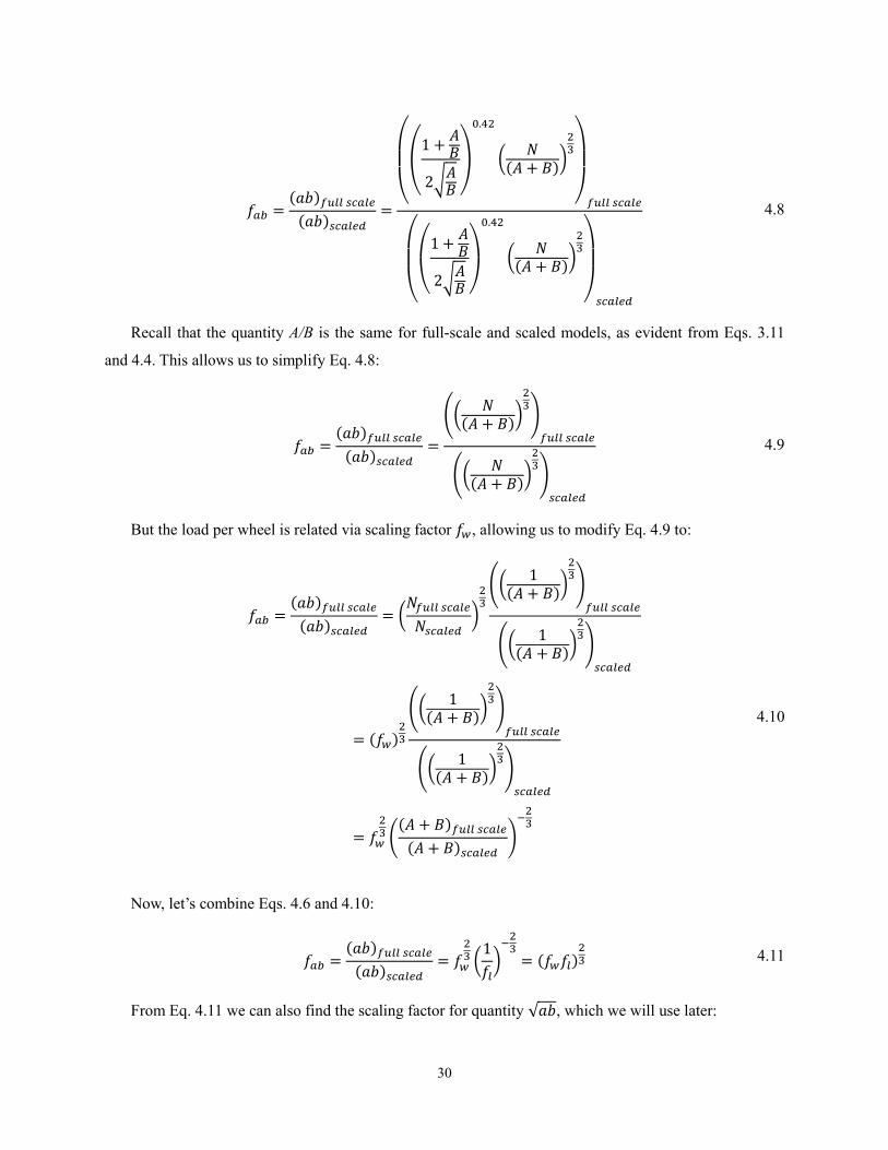
Recall that the quantity A/B is the same for full-scale and scaled models, as evident from Eqs. 3.11

and 4.4. This allows us to simplify Eq. 4.8:


(𝑎𝑏)𝑠𝑐𝑎𝑙𝑒𝑑=

((𝑁

(𝐴 + 𝐵))

23)


((𝑁

(𝐴 + 𝐵))

23)


4.9

But the load per wheel is related via scaling factor 𝑓𝑤, allowing us to modify Eq. 4.9 to:


(𝑎𝑏)𝑠𝑐𝑎𝑙𝑒𝑑= (

𝑁𝑓𝑢𝑙𝑙 𝑠𝑐𝑎𝑙𝑒

𝑁𝑠𝑐𝑎𝑙𝑒𝑑)

23

((1

(𝐴 + 𝐵))

23)


((1

(𝐴 + 𝐵))

23)


= (𝑓𝑤)23

((1

(𝐴 + 𝐵))

23)


((1

(𝐴 + 𝐵))

23)


= 𝑓𝑤

23 (

(𝐴 + 𝐵)𝑓𝑢𝑙𝑙 𝑠𝑐𝑎𝑙𝑒

(𝐴 + 𝐵)𝑠𝑐𝑎𝑙𝑒𝑑)

−23

4.10

Now, let’s combine Eqs. 4.6 and 4.10:


(𝑎𝑏)𝑠𝑐𝑎𝑙𝑒𝑑= 𝑓𝑤

23 (

1

𝑓𝑙)−23= (𝑓𝑤𝑓𝑙)

23 4.11

From Eq. 4.11 we can also find the scaling factor for quantity √𝑎𝑏, which we will use later:

31

𝑓√𝑎𝑏 =√𝑎𝑏𝑓𝑢𝑙𝑙 𝑠𝑐𝑎𝑙𝑒

√𝑎𝑏𝑠𝑐𝑎𝑙𝑒𝑑

= √(𝑎𝑏)𝑓𝑢𝑙𝑙 𝑠𝑐𝑎𝑙𝑒

(𝑎𝑏)𝑠𝑐𝑎𝑙𝑒𝑑= (𝑓𝑤𝑓𝑙)

13 4.12


In the case of longitudinal creepage, combine Eqs. 3.29 and 4.11; recall that c11 only depends on the

b/a ratio, and therefore, the scaling of f11 will be equal to the scaling of the product of ellipse radii a and b:

𝑓𝑓11 =𝑓11,𝑓𝑢𝑙𝑙 𝑠𝑐𝑎𝑙𝑒

𝑓11,𝑠𝑐𝑎𝑙𝑒𝑑=

(−𝐺𝑎𝑏𝑐11)𝑓𝑢𝑙𝑙 𝑠𝑐𝑎𝑙𝑒

(−𝐺𝑎𝑏𝑐11)𝑠𝑐𝑎𝑙𝑒𝑑=

(𝑎𝑏)𝑓𝑢𝑙𝑙 𝑠𝑐𝑎𝑙𝑒


= 𝑓𝑎𝑏 = (𝑓𝑤𝑓𝑙)23

4.13

The same relationship exists for f22 (compare Eqs. 3.29 and 3.30).

For f23, we will combine Eqs. 3.31 and 4.12:

𝑓𝑓23 =𝑓23,𝑓𝑢𝑙𝑙 𝑠𝑐𝑎𝑙𝑒

𝑓23,𝑠𝑐𝑎𝑙𝑒𝑑=

√𝑎𝑏𝑓𝑢𝑙𝑙 𝑠𝑐𝑎𝑙𝑒

√𝑎𝑏𝑠𝑐𝑎𝑙𝑒𝑑

(𝑎𝑏)𝑓𝑢𝑙𝑙 𝑠𝑐𝑎𝑙𝑒

(𝑎𝑏)𝑠𝑐𝑎𝑙𝑒𝑑= 𝑓𝑤𝑓𝑙 4.14

Therefore, if we scale the load per wheel by a factor of 625, and the length by a factor of 5 (as some

authors suggest), creep force per unit creepage will not scale by a factor of 625 [6, 87]. Moreover, the

creepage scaling factor will vary depending on the type of creepage (longitudinal, lateral, or spin).

These results are similar to those obtained by Allen [87].


Similarly to Kalker’s linear theory, we will consider scaling factors under Johnson and Vermeulen’s

theory.

Let us derive the SF for reduced creepages, starting with reduced longitudinal creepage:

𝑓𝜏𝑥 =𝜏𝑥,𝑓𝑢𝑙𝑙 𝑠𝑐𝑎𝑙𝑒

𝜏𝑥,𝑠𝑐𝑎𝑙𝑒𝑑=

(𝐺𝑎𝑏𝑐11𝜈𝑥

3𝜇𝑁 )𝑓𝑢𝑙𝑙 𝑠𝑐𝑎𝑙𝑒


3𝜇𝑁)𝑠𝑐𝑎𝑙𝑒𝑑

=(𝑎𝑏)𝑓𝑢𝑙𝑙 𝑠𝑐𝑎𝑙𝑒


𝑁𝑠𝑐𝑎𝑙𝑒𝑑

𝑁𝑓𝑢𝑙𝑙 𝑠𝑐𝑎𝑙𝑒= (𝑓𝑤𝑓𝑙)

23𝑓𝑤

−1

= 𝑓𝑙

23𝑓𝑤

−13

4.15

Similarly, the SF for reduced lateral creepage is:

32

𝑓𝜏𝑦 =𝜏𝑦,𝑓𝑢𝑙𝑙 𝑠𝑐𝑎𝑙𝑒

𝜏𝑦,𝑠𝑐𝑎𝑙𝑒𝑑= 𝑓𝑙

23𝑓𝑤

−13 4.16

Finally, the SF for reduced total creepage is:

𝑓𝜏 =𝜏𝑓𝑢𝑙𝑙 𝑠𝑐𝑎𝑙𝑒

𝜏𝑠𝑐𝑎𝑙𝑒𝑑=

(√𝜏𝑥2 + 𝜏𝑦

2)𝑓𝑢𝑙𝑙 𝑠𝑐𝑎𝑙𝑒


2)𝑠𝑐𝑎𝑙𝑒𝑑

=√(𝑓𝜏𝑥)

2𝜏𝑥2 + (𝑓𝜏𝑦)

2𝜏𝑦2

√𝜏𝑥2 + 𝜏𝑦

2

=

√(𝑓𝑙

23𝑓𝑤

−13)

2

𝜏𝑥2 + (𝑓𝑙

23𝑓𝑤

−13)

2

𝜏𝑦2


2

= 𝑓𝑙

23𝑓𝑤

−13

4.17

The SF for total creep force is:

𝑓𝐹 =𝐹𝑓𝑢𝑙𝑙 𝑠𝑐𝑎𝑙𝑒

𝐹𝑠𝑐𝑎𝑙𝑒𝑑=

𝜇𝑁(1 − (1 − 𝜏)3)𝑓𝑢𝑙𝑙 𝑠𝑐𝑎𝑙𝑒

𝜇𝑁(1 − (1 − 𝜏)3)𝑠𝑐𝑎𝑙𝑒𝑑

= 𝑓𝑤

1 − (1 − 𝑓𝑙

23𝑓𝑤

−13𝜏)

3

1 − (1 − 𝜏)3

4.18

There are two special cases of this equation, namely pure longitudinal and pure lateral creepage. SF

for longitudinal creep force (under pure longitudinal creepage) is:

𝑓𝐹,𝑥 =

𝐹𝑥,𝑓𝑢𝑙𝑙 𝑠𝑐𝑎𝑙𝑒

𝐹𝑥,𝑠𝑐𝑎𝑙𝑒𝑑= 𝑓𝑤

1 − (1 − 𝑓𝑙

23𝑓𝑤

−13𝜏𝑥)

3

1 − (1 − 𝜏𝑥)3

4.19

The SF for lateral creep force is:

𝑓𝐹,𝑦 =

𝐹𝑦,𝑓𝑢𝑙𝑙 𝑠𝑐𝑎𝑙𝑒

𝐹𝑦,𝑠𝑐𝑎𝑙𝑒𝑑= 𝑓𝑤

1 − (1 − 𝑓𝑙

23𝑓𝑤

−13𝜏𝑦)

3

1 − (1 − 𝜏𝑦)3

4.20

33

Next, recall Eqs. 3.39 to 3.41. We will use these to find SF for saturation creepages (the creepages at

which saturation occurs):

𝑓𝜏𝑥,𝑠𝑎𝑡 =

(3𝜇𝑁

𝐺𝑎𝑏𝑐11)𝑓𝑢𝑙𝑙 𝑠𝑖𝑧𝑒

(3𝜇𝑁

𝐺𝑎𝑏𝑐11)𝑠𝑐𝑎𝑙𝑒𝑑

= 𝑓𝑤(𝑓𝑐11𝑓𝑎𝑏)−1

= 𝑓𝑤 ((𝑓𝑤𝑓𝑙)23)

−1

= 𝑓𝑤

13𝑓𝑙

−23

4.21

𝑓𝜏𝑦,𝑠𝑎𝑡 =

(3𝜇𝑁

𝐺𝑎𝑏𝑐22)𝑓𝑢𝑙𝑙 𝑠𝑖𝑧𝑒

(3𝜇𝑁

𝐺𝑎𝑏𝑐22)𝑠𝑐𝑎𝑙𝑒𝑑

= 𝑓𝑤(𝑓𝑐22𝑓𝑎𝑏)−1

= 𝑓𝑤 ((𝑓𝑤𝑓𝑙)23)

−1

= 𝑓𝑤

13𝑓𝑙

−23

4.22

4.4 Roller Rig vs. Track Correction Factors

4.4.1 Normal Contact

Now consider the relationship between a roller rig and tangent track. Recall the expression for the b/a

ratio given by Eq. 3.26. In the case of a tangent track,

1

𝑟21= 0 4.23

We will introduce the roller rig correction factor, cba, defined as the ratio of the b/a ratios between a

roller rig and tangent track. We derive it by combining Eqs. 3.11 and 3.22:

34

𝑐𝑏𝑎 =

𝑏𝑎𝑟𝑖𝑔

𝑏𝑎𝑡𝑟𝑎𝑐𝑘

=

(

1𝑟11

+1𝑟21

1𝑟12

+1𝑟22

)

0.63

(

1𝑟11

1𝑟12

+1𝑟22

)

0.63 = (

1𝑟11

+1𝑟21

1𝑟11

)

0.63

= (

𝑟21𝑟11𝑟21

+𝑟11

𝑟11𝑟21𝑟21

𝑟11𝑟21

)

0.63

= (𝑟11 + 𝑟21

𝑟21)0.63

4.24

Two additional correction factors are derived from Eqs. 3.1and 3.2; we will use them when defining

correction factors for Kalker’s coefficients:

𝑐𝐴𝐵 =

𝐴𝐵𝑟𝑖𝑔

𝐴𝐵𝑡𝑟𝑎𝑐𝑘

=

12(

1𝑟11

+1𝑟21

)

12 (

1𝑟12

+1𝑟22

)=

𝑟11 + 𝑟21

𝑟21 4.25

𝑐𝐴+𝐵 =(𝐴 + 𝐵)𝑟𝑖𝑔

(𝐴 + 𝐵)𝑡𝑟𝑎𝑐𝑘=

12(

1𝑟11

+1𝑟21

+1𝑟12

+1𝑟22

)𝑟𝑖𝑔

12(

1𝑟11

+1𝑟21

+1𝑟12

+1𝑟22

)𝑡𝑟𝑎𝑐𝑘

=

1𝑟11

+1𝑟12

+1𝑟21

+1𝑟22

1𝑟11

+1𝑟12

+1𝑟22

4.26

Finally, we will introduce a correction factor for the quantity ab. It is derived similar to the scaling

factor for the same quantity in Eqs. 4.7 and 4.8, except that the quality A/B is not the same in a roller rig

and tangent track. Hence, the result is more complex:

35

𝑐𝑎𝑏 =𝑎𝑏𝑟𝑖𝑔

𝑎𝑏𝑡𝑟𝑎𝑐𝑘=

(

(

1 +

𝐴𝐵

2√𝐴𝐵 )

0.42

(1

𝑐𝐴+𝐵 (𝐴 + 𝐵))

23

)

𝑟𝑖𝑔

(

(

1 +

𝐴𝐵

2√𝐴𝐵 )

0.42

(1

(𝐴 + 𝐵))

23

)

𝑡𝑟𝑎𝑐𝑘

=(

1 + 𝑐𝐴𝐵

𝐴𝐵

2√𝑐𝐴𝐵 𝐴𝐵 )

0.42

(1

𝑐𝐴+𝐵 (𝐴 + 𝐵))

23

(

1 +

𝐴𝐵

2√𝐴𝐵 )

0.42

(1

(𝐴 + 𝐵))

23

= ((1 + 𝑐𝐴𝐵

𝐴𝐵)

√𝑐𝐴𝐵 (1 +𝐴𝐵)

)

0.42

𝑐𝐴+𝐵 −23

4.27


Correction factors for c11, c22, and c23 are calculated from Eqs. 3.23 to 3.25; note that b/a, A/B, and

(A+B) values are for a tangent track, unless specified otherwise:

𝑐𝑐11 =𝑐11,𝑟𝑖𝑔

𝑐11,𝑡𝑟𝑎𝑐𝑘 =

3.2893 +0.975

𝑐𝑏𝑎𝑏𝑎

−0.012

(𝑐𝑏𝑎𝑏𝑎)

2

3.2893 +0.975

𝑏𝑎

−0.012

(𝑏𝑎)

2

4.28



2.4014 +1.3179


−0.02

(𝑐𝑏𝑎𝑏𝑎)

2

2.4014 +1.3179

𝑏𝑎

−0.02

(𝑏𝑎)

2

4.29

36



0.4147 +1.0184


+0.0565

(𝑐𝑏𝑎𝑏𝑎)2 −

0.0013

(𝑐𝑏𝑎𝑏𝑎)3

0.4147 +1.0184

𝑏𝑎

+0.0565

(𝑏𝑎)2 −

0.0013

(𝑏𝑎)3

4.30

The correction factor for f11 is calculated similar to the scaling factor in Eq. 4.13:

𝑐𝑓11 =𝑓11,𝑟𝑖𝑔

𝑓11,𝑡𝑟𝑎𝑐𝑘=

(−𝐺𝑎𝑏𝑐11)𝑟𝑖𝑔(−𝐺𝑎𝑏𝑐11)𝑡𝑟𝑎𝑐𝑘

= 𝑐𝑐11

(𝑎𝑏)𝑟𝑖𝑔(𝑎𝑏)𝑡𝑟𝑎𝑐𝑘

= 𝑐𝑐11𝑐𝑎𝑏

4.31

Similarly, for f22 and f23:

𝑐𝑓22 = 𝑐𝑐22𝑐𝑎𝑏 4.32

𝑐𝑓23 = 𝑐𝑐23(𝑐𝑎𝑏)32 4.33


Now consider Johnson and Vermeulen’s theory. We first derive correction factors for reduced

longitudinal and lateral creepages:

𝑐𝜏𝑥 =𝜏𝑥,𝑟𝑜𝑙𝑙𝑒𝑟

𝜏𝑥,𝑡𝑟𝑎𝑐𝑘 =


3𝜇𝑁 )𝑟𝑜𝑙𝑙𝑒𝑟


3𝜇𝑁)𝑡𝑟𝑎𝑐𝑘

= 𝑐𝑎𝑏𝑐𝑐11 4.34

𝑐𝜏𝑦 =𝜏𝑦,𝑟𝑜𝑙𝑙𝑒𝑟

𝜏𝑦,𝑡𝑟𝑎𝑐𝑘 =

(𝐺𝑎𝑏𝑐22𝜈𝑦

3𝜇𝑁 )𝑟𝑜𝑙𝑙𝑒𝑟

(𝐺𝑎𝑏𝑐22𝜈𝑦

3𝜇𝑁 )𝑡𝑟𝑎𝑐𝑘

= 𝑐𝑎𝑏𝑐𝑐22 4.35

Next, we derive the CF for total reduced creepage:

37

𝑐𝜏 =𝜏𝑟𝑜𝑙𝑙𝑒𝑟

𝜏𝑡𝑟𝑎𝑐𝑘=


2)𝑟𝑜𝑙𝑙𝑒𝑟


2)𝑡𝑟𝑎𝑐𝑘

=√𝑐𝜏𝑥

2 𝜏𝑥2 + 𝑐𝜏𝑦

2 𝜏𝑦2


2

=√𝑐𝑎𝑏

2 𝑐𝑐112 𝜏𝑥

2 + 𝑐𝑎𝑏2 𝑐𝑐22

2 𝜏𝑦2


2

=

𝑐𝑎𝑏√𝑐𝑐112 𝜏𝑥

2 + 𝑐𝑐222 𝜏𝑦

2


2

4.36

Based on the above, we define the CF for the total friction force before saturation:

𝑐𝐹 =(1 − (1 − 𝜏)3)𝑟𝑖𝑔

(1 − (1 − 𝜏)3)𝑡𝑟𝑎𝑐𝑘=

1 − (1 − 𝑐𝜏𝜏)3

1 − (1 − 𝜏)3 4.37

The correction factor for traction force (longitudinal creepage) is:

𝑐𝐹𝑥 =(1 − (1 − 𝜏𝑥)

3)𝑟𝑖𝑔(1 − (1 − 𝜏𝑥)

3)𝑡𝑟𝑎𝑐𝑘=

1 − (1 − 𝑐𝜏𝑥𝜏𝑥)3

1 − (1 − 𝜏𝑥)3

=1 − (1 − 𝑐𝑎𝑏𝑐𝑐11𝜏𝑥)

3

1 − (1 − 𝜏𝑥)3

=1 − (1 − 𝑐𝑎𝑏𝑐𝑐11

𝐺𝑎𝑏𝑐11𝜈𝑥3𝜇𝑁 )

3

1 − (1 −𝐺𝑎𝑏𝑐11𝜈𝑥

3𝜇𝑁)3

4.38

Similarly, the CF for traction forces due to pure lateral creepage is:

38

𝑐𝐹𝑦 =

(1 − (1 − 𝜏𝑦)3)𝑟𝑖𝑔

(1 − (1 − 𝜏𝑦)3)𝑡𝑟𝑎𝑐𝑘

=1 − (1 − 𝑐𝜏𝑦𝜏𝑦)

3

1 − (1 − 𝜏𝑦)3

=1 − (1 − 𝑐𝑎𝑏𝑐𝑐22𝜏𝑦)

3

1 − (1 − 𝜏𝑦)3

=1 − (1 − 𝑐𝑎𝑏𝑐𝑐22


3𝜇𝑁 )3

1 − (1 −𝐺𝑎𝑏𝑐22𝜈𝑦

3𝜇𝑁)3

4.39

Again, we use Eqs. 3.39 to 3.41 to find the CF for the saturation point, in pure longitudinal or pure

lateral creepage, respectively:

𝑐𝜏𝑥,𝑠𝑎𝑡 =

(3𝜇𝑁

𝐺𝑎𝑏𝑐11)𝑟𝑖𝑔

(3𝜇𝑁

𝐺𝑎𝑏𝑐11)𝑡𝑟𝑎𝑐𝑘

=

3𝜇𝑁𝐺𝑐𝑎𝑏𝑎𝑏𝑐𝑐11𝑐11

3𝜇𝑁𝐺𝑎𝑏𝑐11

= (𝑐𝑎𝑏𝑐𝑐11)−1 4.40

𝑐𝜏𝑦,𝑠𝑎𝑡 =

(3𝜇𝑁

𝐺𝑎𝑏𝑐22)𝑟𝑖𝑔

(3𝜇𝑁

𝐺𝑎𝑏𝑐22)𝑡𝑟𝑎𝑐𝑘

=

3𝜇𝑁𝐺𝑐𝑎𝑏𝑎𝑏𝑐𝑐22𝑐22

3𝜇𝑁𝐺𝑎𝑏𝑐22

= (𝑐𝑎𝑏𝑐𝑐22)−1 4.41

4.5 Transformation Factors


We will now combine the scaling factors for creep forces and roller-to-track correction factors into

what we will call transformation factors (TF). As explained earlier, these variables will describe the creep

force ratios between a scaled roller rig and a full-size tangent track. We will define them as:

𝑇𝑓11 =𝑓11,𝑠𝑐𝑎𝑙𝑒𝑑 𝑟𝑜𝑙𝑙𝑒𝑟 𝑟𝑖𝑔

𝑓11,𝑓𝑢𝑙𝑙 𝑠𝑖𝑧𝑒 𝑡𝑟𝑎𝑐𝑘=

𝑓11,𝑠𝑐𝑎𝑙𝑒𝑑

𝑓11,𝑓𝑢𝑙𝑙 𝑠𝑐𝑎𝑙𝑒

𝑓11,𝑟𝑖𝑔


1

𝑓𝑓11𝑐𝑓11

= (𝑓𝑤𝑓𝑙)−23 𝑐𝑓11

4.42

39





𝑓22,𝑟𝑖𝑔


1


= (𝑓𝑤𝑓𝑙)−23 𝑐𝑓22

4.43





𝑓23,𝑟𝑖𝑔


1


= (𝑓𝑤 𝑓𝑙)−1 𝑐𝑓23

4.44


The transformation factor for total creep force is given by:

𝑇𝐹 =𝐹𝑟𝑜𝑙𝑙𝑒𝑟

𝐹𝑡𝑟𝑎𝑐𝑘

𝐹𝑠𝑐𝑎𝑙𝑒𝑑

𝐹𝑓𝑢𝑙𝑙 𝑠𝑐𝑎𝑙𝑒= 𝑐𝐹(𝑓𝐹)

−1

=1 − (1 − 𝑐𝜏𝜏)

3

1 − (1 − 𝜏)31 − (1 − 𝜏)3

1 − (1 − 𝑓𝑙

23𝑓𝑤

−13𝜏)

3

=1 − (1 − 𝑐𝜏𝜏)

3

1 − (1 − 𝑓𝑙

23𝑓𝑤

−13𝜏)

3

4.45

In a purely longitudinal creepage:

𝑇𝐹,𝑥 =𝐹𝑥,𝑟𝑖𝑔

𝐹𝑥,𝑡𝑟𝑎𝑐𝑘

𝐹𝑥,𝑠𝑐𝑎𝑙𝑒𝑑

𝐹𝑥,𝑓𝑢𝑙𝑙 𝑠𝑐𝑎𝑙𝑒= 𝑐𝐹,𝑥(𝑓𝐹,𝑥)

−1 4.46

In a purely lateral creepage:

𝑇𝐹,𝑦 =𝐹𝑦,𝑟𝑖𝑔

𝐹𝑦,𝑡𝑟𝑎𝑐𝑘

𝐹𝑦,𝑠𝑐𝑎𝑙𝑒𝑑

𝐹𝑦,𝑓𝑢𝑙𝑙 𝑠𝑐𝑎𝑙𝑒= 𝑐𝐹,𝑦(𝑓𝐹,𝑦)

−1 4.47

Where the appropriate SF and CF are as defined earlier.

The TF for saturation creepages (pure longitudinal and pure lateral cases):

40

𝑇𝜏𝑥,𝑠𝑎𝑡 =𝜏𝑥,𝑠𝑎𝑡,𝑟𝑖𝑔

𝜏𝑥,𝑠𝑎𝑡,𝑡𝑟𝑎𝑐𝑘

𝜏𝑥,𝑠𝑎𝑡,𝑠𝑐𝑎𝑙𝑒𝑑

𝜏𝑥,𝑠𝑎𝑡,𝑓𝑢𝑙𝑙 𝑠𝑐𝑎𝑙𝑒= 𝑐𝜏𝑥,𝑠𝑎𝑡𝑓𝜏𝑥,𝑠𝑎𝑡

−1

= (𝑐𝑎𝑏𝑐𝑐11)−1 (𝑓𝑤

13𝑓𝑙

−23)

−1

= (𝑐𝑎𝑏𝑐𝑐11)−1𝑓𝑤

−13𝑓𝑙

23

4.48

𝑇𝜏𝑦,𝑠𝑎𝑡 =𝜏𝑦,𝑠𝑎𝑡,𝑟𝑖𝑔

𝜏𝑦,𝑠𝑎𝑡,𝑡𝑟𝑎𝑐𝑘

𝜏𝑦,𝑠𝑎𝑡,𝑠𝑐𝑎𝑙𝑒𝑑

𝜏𝑦,𝑠𝑎𝑡,𝑓𝑢𝑙𝑙 𝑠𝑐𝑎𝑙𝑒= 𝑐𝜏𝑦,𝑠𝑎𝑡𝑓𝜏𝑦,𝑠𝑎𝑡

−1

= (𝑐𝑎𝑏𝑐𝑐22)−1 (𝑓𝑤

13𝑓𝑙

−23)

−1

= (𝑐𝑎𝑏𝑐𝑐22)−1𝑓𝑤

−13𝑓𝑙

23

4.49

4.6 Influence of Specific Scaling Strategies

4.6.1 General Remarks

As we showed earlier, the scaling factors for creep forces per unit creepage describe the relationship

expressed in Eqs. 4.13 to 4.14. That is, they always scale by a different factor than the normal load per

wheel (except in the trivial case where length scaling factor is 1).

As we approach saturation, however, creep forces can be described by the Coulomb law:

𝐹𝐶𝑜𝑢𝑙𝑜𝑚𝑏 = 𝜇𝑁 4.50

Consequently, under saturation, the scaling factor for longitudinal friction force will exhibit a more

straightforward relationship to the weight scaling factor:

𝑓𝐹,𝐶𝑜𝑢𝑙𝑜𝑚𝑏 = 𝑓𝜇𝑓𝑤 4.51

Now let us consider the specific way different scaling strategies work [6, 87].

41

4.6.2 MMU’s Strategy

The roller rig at Manchester Metropolitan University (MMU) was built in 1992m and has been used

to study the dynamic behavior of rail vehicles. Since the overall dynamics, rather than creep forces, were

the focus of the studies, the strategy used on this rig was based on the similarity of equation of motion

(EOM).

The researchers set the time SF at 1 to ease the analysis of data in terms of time and spectrum [6, 87].

𝑓𝑡 = 1 4.52

Length scaling factor was set at 5.

𝑓𝑙 = 5 4.53

The same scaling factor, then, is used for displacement.

Based on time and displacement SF, scaling factors for velocity and linear acceleration are,

respectively,

𝑓𝑣 =𝑓𝑙𝑓𝑡

= 5 4.54

𝑓𝑎 =𝑓𝑙

𝑓𝑡2 = 5

4.55

The same material (steel) was used for wheels and rollers that is normally used in the railroad

industry, forcing the scaling factors for friction coefficient, Young’s modulus, density, and Poisson’s ratio

to be 1:

𝑓𝜇 = 1 4.56

𝑓𝐸 = 1 4.57

𝑓𝜌 = 1 4.58

𝑓𝑃𝑅 = 1 4.59

Scaling factors for mass and moment of inertia are, consequently,

𝑓𝑚 = 𝑓𝜌𝑓𝑙3 = 125 4.60

42

𝑓𝐼 = 𝑓𝑚𝑓𝑙2 = 3125 4.61

We now turn to basic translational and rotational equations of motion:

𝑚�� + 𝑐�� + 𝑘𝑥 = 𝐹 4.62

𝐼�� + 𝑐𝑇�� + 𝑘𝑇𝜃 = 𝑇 4.63

Considering the scaling factors, these equations become:

𝑚��(𝑓𝑚𝑓𝑎) + 𝑐��(𝑓𝑐𝑓𝑣) + 𝑘𝑥(𝑓𝑘𝑓𝑙) = 𝐹(𝑓𝐹) 4.64

𝐼��(𝑓𝐼𝑓𝑡−2) + 𝑐𝑇��(𝑓𝑐𝑇𝑓𝑡

−1) + 𝑘𝑇𝜃(𝑓𝑘𝑇) = 𝑇(𝑓𝑇) 4.65

It is worth noting that Allen assumes a scaling factor 𝑓𝑘𝑇𝑓𝑡−1 for elastic forces, for reasons

unbeknown to the author. This selection, however, does not change the results of this study since time

scaling factor equals 1.

In order for the EOM of the scaled rig to be similar to that of a full-size system, all the applied forces

(inertial forces, elastic forces, damping forces) must have the same scaling factors:

𝑓𝑚𝑓𝑎 = 𝑓𝑐𝑓𝑣 = 𝑓𝑘𝑓𝑙 = 𝑓𝐹𝑜𝑟𝑐𝑒 4.66

𝑓𝐼𝑓𝑡−2 = 𝑓𝑐𝑇𝑓𝑡

−1 = 𝑓𝑘𝑇 = 𝑓𝑇 4.67

Combining Eq. 4.66 with Eqs. 4.50 to 4.60 yields:

𝑓𝜌𝑓𝑙3

𝑓𝑙

𝑓𝑡2 = 𝑓𝑐

𝑓𝑙𝑓𝑡

= 𝑓𝑘𝑓𝑙 = 𝑓𝐹𝑜𝑟𝑐𝑒 4.68

That can be further simplified to:

𝑓𝜌𝑓𝑙4𝑓𝑡

−2 = 𝑓𝑐𝑓𝑙𝑓𝑡−1 = 𝑓𝑘𝑓𝑙 = 𝑓𝐹𝑜𝑟𝑐𝑒 4.69

When we assign the time and density SF to be 1, we obtain:

𝑓𝑙4 = 𝑓𝑐𝑓𝑙 = 𝑓𝑘𝑓𝑙 = 𝑓𝐹𝑜𝑟𝑐𝑒 4.70

Similarly, when we combine 4.67 with 4.50 to 4.60, we obtain:


−2 = 𝑓𝑐𝑇𝑓𝑡−1 = 𝑓𝑘𝑇 = 𝑓𝑇 4.71

Which can be simplified to:

43


−2 = 𝑓𝑐𝑇𝑓𝑡−1 = 𝑓𝑘𝑇 = 𝑓𝑇 4.72

𝑓𝑙5 = 𝑓𝑐𝑇 = 𝑓𝑘𝑇 = 𝑓𝑇 4.73

Notice that 𝑓𝐹𝑜𝑟𝑐𝑒, the scaling factor for inertial, elastic, and damping forces, is not necessary equal to

𝑓𝐹, the scaling factor for creep force.

If we compare Eqs. 4.70 and 6.26, we see that, unsurprisingly, the SF for torque and force (and those

for linear and torsional stiffness, as well as linear and torsional damping) are related to each other via the

length SF.

The combined external forces term F includes gravitational, creepage and any other forces applied

onto the wheelset (note: the gravitational force is included because it can influence creep forces). Herein

lies the problem: since SF for acceleration is 5, but the gravitational acceleration cannot be scaled,

gravitational forces do not scale by the same factor as inertial, elastic, or damping forces.

Recall that if length SF is 5 for the chosen scaling strategy, the inertial forces are scaled by 625, while

the gravitational forces are scaled by 125. It appears, then, that this scaling strategy does not allow for an

accurate representation of the dynamic behavior of a wheelset, unless some external force is applied to

“simulate” gravitational forces.

Furthermore, if the assumed external force is applied, we will need to consider how it would affect

the creep forces.

Recall from Eq. 4.13 that under Kalker’s linear theory, the creep force per unit creepage is scaled by a

factor of (𝑓𝑤𝑓𝑙)

, where 𝑓𝑤 is the normal force per wheel. However, this normal force may have both

gravitational and inertial components.

If we consider the gravitational component of the normal force,

𝑓𝑓11 = (𝑓𝑤𝑓𝑙)23 = (𝑓𝑚𝑓𝑔𝑓𝑙)

23 = (𝑓𝜌𝑓𝑙

3𝑓𝑔𝑓𝑙)23 = (𝑓𝑙

4)23 = 𝑓𝑙

223

= 73.10

4.74

If we consider the inertial component,

𝑓𝑓11 = (𝑓𝑤𝑓𝑙)23 = (𝑓𝑚𝑓𝑎𝑓𝑙)


3𝑓𝑙

𝑓𝑡2 𝑓𝑙)

23

= (𝑓𝑙5)

23 = 𝑓𝑙

313

= 213.75

4.75

44

The difference, as we see it, is quite substantial.

4.6.3 DLR’s Strategy

Since one of the main purposes for the DLR’s rig was the study of hunting oscillations, the scaling

strategy chosen for this rig was based upon the similarity of lateral equation of motion of a suspended

dicone, which represents a wheelset [6, 87].

𝑚

𝜒�� =

𝐼𝑦𝛤𝑉

𝜒𝑟0�� −

𝑚𝑔𝑏0

𝜒𝑦 −

2𝑘𝑦

𝜒𝑦 + 𝐹𝑦 + 𝐹𝑥𝜓 4.76

In this equation, m is wheelset mass, 𝑦 is lateral displacement, 𝜓 is yaw displacement, 𝑘𝑦 is lateral

stiffness, 𝑉 is full-scale system volume, 𝐼𝑦 is the wheelset’s rotational inertia around y-axis, Fx and Fy are

longitudinal and lateral creep forces, and 𝛤 is a geometric parameter defined as:

𝛤 =𝛾

𝑙0− 𝑟𝑜𝛾 4.77

Where 𝑙0 is half-gauge, χ is the leading angle defined as:

𝜒 =𝛤𝑙0𝛾

4.78

And b0 is a geometric quality defined as:

𝑏0 = 2𝛤 + 𝛤2(𝑟0 + 𝑟21) 4.79

The scaled rig’s corresponding equation is:

𝑚

𝜒��

𝑓𝑚𝑓𝑙

𝑓𝑡2 =

𝐼𝑦𝛤𝑉

𝜒𝑟0��

𝑓𝑚𝑓𝑙2𝑓𝑉

𝑓𝑡𝑓𝑙2 −

𝑚𝑔𝑏0

𝜒𝑦𝑓𝑚 −

2𝑘𝑦

𝜒𝑦𝑓𝑙𝑓𝑘 + 𝐹𝑦𝑓𝑇

+ 𝐹𝑥𝜓𝑓𝑇

4.80

Dividing Eq. 6.26 by 𝑓 𝑓

𝑓 yields:

𝑚

𝜒�� =

𝐼𝑦𝛤𝑉

𝜒𝑟0�� −

𝑚𝑔𝑏0

𝜒𝑦

𝑓𝑡2

𝑓𝑙 −

2𝑘𝑦

𝜒𝑦

𝑓𝑘𝑓𝑡2

𝑓𝑚

+ (𝐹𝑦 + 𝐹𝑥𝜓)𝑓𝐹𝑓𝑙

2

𝑓𝑚𝑓𝑙

4.81

45

In order for a scaled roller rig to be dynamically similar to the full-size rig, three conditions must be

met:

Velocity scaling:

𝑓𝑡

2

𝑓𝑙= 1 → 𝑓𝑉 = √𝑓𝑙 4.82

Stiffness scaling:

𝑓𝑘𝑓𝑡

2

𝑓𝑚= 1 → 𝑓𝑘 = 𝑓𝜌𝑓𝑙

2 4.83

Creep force scaling:

𝑓𝐹𝑓𝑡

2

𝑓𝑚𝑓𝑙= 1 → 𝑓𝐹 = 𝑓𝜌𝑓𝑙

3 4.84

Now we can compute the scaling factors for acceleration, mass, etc.:

𝑓𝑡 =𝑓𝑙𝑓𝑉

=𝑓𝑙

√𝑓𝑙= √𝑓𝑙 4.85

𝑓𝑎 =𝑓𝑉𝑓𝑡

=√𝑓𝑙

√𝑓𝑙= 1 4.86

Because acceleration SF is 1, unlike in MMU’s strategy, scaling factors for gravitational and inertial

forces are identical to those for creep forces:

𝑓𝑚𝑔 = 𝑓𝑚𝑎 = 𝑓𝜌𝑓𝑙3 4.87

Recall, however, that from 4.13, longitudinal and lateral creep forces (assuming Kalker’s linear theory

before saturation) must be:

𝑓𝐹 = 𝑓𝑓11 = 𝑓𝑓22 = (𝑓𝑤𝑓𝑙)23 4.88

Eqs. 4.87 and 6.26 mean that:

𝑓𝐹 = (𝑓𝑤𝑓𝑙)23 = (𝑓𝑚𝑔𝑓𝑙)


3𝑓𝑙)23 = 𝑓𝜌

23𝑓𝑙

223 4.89

It is only compatible with Eq. 4.84 if:

46

𝑓𝜌 =1

𝑓𝑙 4.90

If length SF of 5 is used (as it is in the DLR rig), then that would require density SF of 0.2, which is

difficult to achieve. Jaschinski solves this problem by using an SF of 0.5. If density SF of 0.5 is used

along with length SF of 5, then creep force SF is 62.5 according to Eq. 4.84, but is 46.1 according to

Eq. 4.89. DLR deemed this to be acceptable because exact scaling of contact patch is important at low

creepages, but is not necessary for limit cycle analysis, since under those conditions, contact patch is

saturated. Allen notes that the use of this SF led to good experimental results.

Something to consider is whether it would be appropriate to apply external force (e.g., via hydraulic

actuators) and thus vary the normal force independently of gravitational and inertial forces. It appears that

in this case, the similarity of lateral dynamics will be preserved as long as the normal force is scaled

according to Eqs. 4.84 and 4.13:

(𝑓𝑤𝑓𝑙)23 = 𝑓𝜌𝑓𝑙

3 → 𝑓𝑤 = 𝑓𝜌1.5𝑓𝑙

3.5 4.91

4.6.4 INRETS’ Strategy

Since the main objective of INRETS’ rig was the study of wheel-rail contact, its creators decided to

base the scaling on the similarity of stresses everywhere in the system, including contact patch and elastic

components (which also simplifies the design of suspension components) [6, 87]:

𝑓𝜎 =𝑓𝐹𝑜𝑟𝑐𝑒

𝑓𝑙2 = 1 4.92

In addition, INRETS’ strategy involves the use of the same material in the scaled rig that would be

used in a full-scale device:

𝑓𝜌 = 𝑓𝐸 = 𝑓𝑃𝑅 = 1 4.93

Eq. 4.92 means that the general force scaling factor is:

𝑓𝐹𝑜𝑟𝑐𝑒 = 𝑓𝑙2 4.94

Based on density and length scaling factors, one can derive the mass scaling factor:

𝑓𝑚 = 𝑓𝜌𝑓𝑙3 = 𝑓𝑙

3 4.95

Since gravitational acceleration cannot be scaled, gravitational force scales as:

47

𝑓𝑚𝑔 = 𝑓𝑙3 4.96

The stiffness scaling factor is then computed:

𝑓𝑘 =𝑓𝐹𝑜𝑟𝑐𝑒

𝑓𝑙=

𝑓𝑙2

𝑓𝑙= 𝑓𝑙 4.97

The frequency scaling factor, therefore, is:

𝑓𝑓𝑟𝑒𝑞 = √𝑓𝑘𝑓𝑚

= √𝑓𝑙

𝑓𝑙3 =

1

𝑓𝑙 4.98

This forces the time scaling factor to be:

𝑓𝑡 =1

𝑓𝑓𝑟𝑒𝑞= 𝑓𝑙 4.99

Knowing the time and length scaling factors, we can compute the velocity and acceleration scaling

factors:

𝑓𝑉 =𝑓𝑙𝑓𝑡

=𝑓𝑙𝑓𝑙

= 1 4.100

𝑓𝑎 =𝑓𝑉𝑓𝑡

=1

𝑓𝑙 4.101

This means that the inertial forces will scale differently from the gravitational forces:

𝑓𝑚𝑎 = 𝑓𝑚𝑓𝑎 = 𝑓𝑙3𝑓𝑙

−1 = 𝑓𝑙2 4.102

As with other strategies, this can be solved by “simulating” gravitational forces with actuators.

Recall the scaling of creep forces under Kalker’s linear model, as predicted by Eq. 4.13; given the

inertial and elastic force scaling chosen, this means:

(𝑓𝑤𝑓𝑙)23 = 𝑓𝐹 = 𝑓𝑚𝑎 = 𝑓𝑘𝑥 = 𝑓𝑙

2 4.103

Solving for normal force SF:

𝑓𝑤 = 𝑓𝑙2 4.104

This expression, in essence, explains what force should be applied in order for creep force to scale

similarly to inertial and elastic forces.

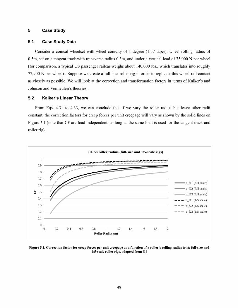
48

5 Case Study

5.1 Case Study Data

Consider a conical wheelset with wheel conicity of 1 degree (1:57 taper), wheel rolling radius of

0.5m, set on a tangent track with transverse radius 0.3m, and under a vertical load of 75,000 N per wheel

(for comparison, a typical US passenger railcar weighs about 140,000 lbs., which translates into roughly

77,900 N per wheel) . Suppose we create a full-size roller rig in order to replicate this wheel-rail contact

as closely as possible. We will look at the correction and transformation factors in terms of Kalker’s and

Johnson and Vermeulen’s theories.

5.2 Kalker’s Linear Theory

From Eqs. 4.31 to 4.33, we can conclude that if we vary the roller radius but leave other radii

constant, the correction factors for creep forces per unit creepage will vary as shown by the solid lines on

Figure 5.1 (note that CF are load independent, as long as the same load is used for the tangent track and

roller rig).

Figure 5.1. Correction factor for creep forces per unit creepage as a function of a roller’s rolling radius (r21): full-size and

1/5-scale roller rigs, adapted from [1]

0

0.1

0.2

0.3

0.4

0.5

0.6

0.7

0.8

0.9

1

0 0.2 0.4 0.6 0.8 1 1.2 1.4 1.6 1.8 2

CF

Roller Radius (m)

CF vs roller radius (full-size and 1/5-scale rigs)

c_f11 (full scale)

c_f22 (full scale)

c_f23 (full scale)

c_f11 (1/5 scale)

c_f22 (1/5 scale)

c_f23 (1/5 scale)

49

When we are using a full-size roller rig, i.e. length SF and load SF are equal to 1, the transformation

factors will be identical to the correction factors (Eqs. 4.42 to 4.44), as shown by the solid lines on

Figure 5.2.

Figure 5.2. TF for creep forces per unit creepage as a function of a roller radius: full-size and 1/5-scale roller rigs, adapted

from [1]

Note that the TF and CF for f23 differ significantly from the TF and CF for f11 and f22. This is due to

the fact that, as discussed earlier, the longitudinal and lateral creepages are dimensionless, while spin

creepage, by default, has units of m-1

. If we were seeking CF and TF for creep forces per unit of

normalized spin creepage, then they would not vary nearly as drastically from other CF and TF.

Suppose we now try to create a scaled roller rig according to INRETS’ strategy. We scale all

dimensions by a factor of 5, and the load by a factor of 25 (recall that INRETS’ strategy is designed to

keep the pressure in the contact patch constant so that creep forces are scaled by the same factor as the

vertical load). We then replace the tangent track with a roller to see how CF vary with roller radius.

As the dashed lines on Figure 5.1 show, for the same roller diameter, one can get a much higher

correction factor for the scaled roller rig than for a full-size rig. Although scaling factors do not directly

appear in the expressions for correction factors, we must remember that in Figure 5.1, we change roller

0

0.005

0.01

0.015

0.02

0.025

0.03

0.035

0.04

0

0.1

0.2

0.3

0.4

0.5

0.6

0.7

0.8

0.9

1

0 0.5 1 1.5 2 2.5

TF

(1

/5 s

cale

)

TF

(fu

ll s

ize)

Roller Radius (m)

TF vs. roller radius (full-size and 1/5-scale rigs)

T_f11 (full scale)

T_f22 (full scale)

T_f23 (full scale)

T_f11 (1/5 scale)

T_f22 (1/5 scale)

T_f23 (1/5 scale)

50

radius independently of scaling. If we scaled all dimensions, including the roller radius, by a factor of 5,

CF would be the same as for a full-size rig.

Since length SF is 5 and load SF is 25, transformation factors, unlike correction factors, will be far

from 1 (Figure 5.2).

Another way to examine CF and TF would be to scale all lengths in the roller rig, including roller

diameter, by the length scaling factor fl, while scaling the load according to INRETS’ strategy (𝑓𝑤 = 𝑓𝑙2).

The contact patch will have the same shape (b/a ratio), regardless of length SF, so CF for f11, f22, and f23

will remain 0.72, 0.68, and 0.51, respectively. TF, predictably, will decrease when length SF increases, as

seen in Figure 5.3.

Figure 5.3. Transformation factor for creep forces per unit creepage as a function of length SF, adapted from [1]

Another way of tracking the changes in CF and TF would be by plotting them against the ratio of

wheel radius to roller radius. In this case, as Figure 5.4 shows, length scaling factor (1 or 5) does not

matter in terms of CF; what makes the difference is the ratio of the radii. The lower this ratio is, the more

closely the roller rig represents a tangent track. On the other hand, TF will vary between 1/5-scale and

full-size rigs, as seen in Figure 5.5.

0

0.1

0.2

0.3

0.4

0.5

0.6

0.7

0.8

1 1.5 2 2.5 3 3.5 4 4.5 5

CF

, T

F

fl

CF and TF: dependence on length SF

c_f11

c_f22

c_f23

T_f11

T_f22

T_f23

51

Figure 5.4. Correction factor for creep forces per unit creepage as a function of wheel and roller radii ratio: full-size and

1/5-scale roller rigs, adapted from [1]

Figure 5.5. Transformation factor for creep forces per unit creepage as a function of wheel and roller radii ratio: full-size

and 1/5-scale roller rigs, adapted from [1]

0.5

0.55

0.6

0.65

0.7

0.75

0.8

0.85

0.9

0.95

1

0 0.1 0.2 0.3 0.4 0.5 0.6 0.7 0.8 0.9 1

CF

r11/r21

CF vs wheel and roller radii ratio (full-size and 1/5-scale rigs)

c_f11 (full scale)

c_f22 (full scale)

c_f23 (full scale)

c_f11 (1/5 scale)

c_f22 (1/5 scale)

c_f23 (1/5 scale)

0

0.005

0.01

0.015

0.02

0.025

0.03

0.035

0.04

0

0.1

0.2

0.3

0.4

0.5

0.6

0.7

0.8

0.9

1

0.2 0.3 0.4 0.5 0.6 0.7 0.8 0.9 1

TF

(fu

ll s

ize)

r11/r21

TF vs. wheel and roller radii ratio (full-size and 1/5-scale)

T_f11 (full scale)

T_f22 (full scale)

T_f23 (full scale)

T_f11 (1/5 scale)

T_f22 (1/5 scale)

T_f23 (1/5 scale)

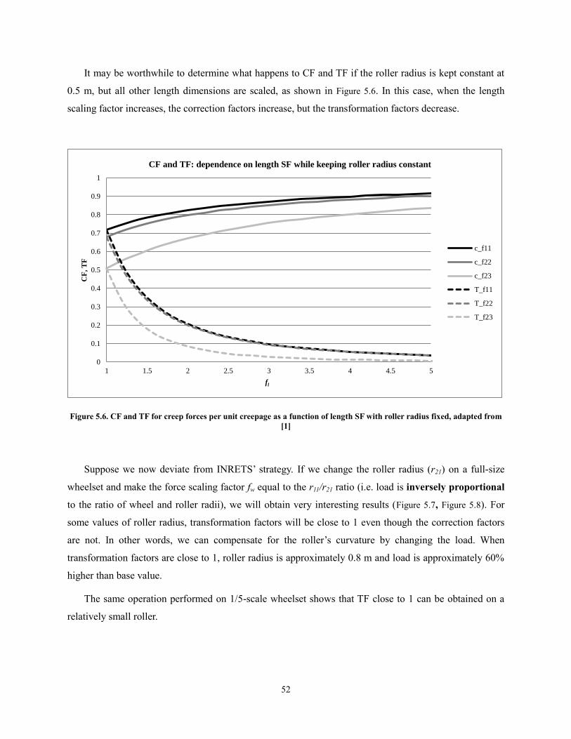
52

It may be worthwhile to determine what happens to CF and TF if the roller radius is kept constant at

0.5 m, but all other length dimensions are scaled, as shown in Figure 5.6. In this case, when the length

scaling factor increases, the correction factors increase, but the transformation factors decrease.

Figure 5.6. CF and TF for creep forces per unit creepage as a function of length SF with roller radius fixed, adapted from

[1]

Suppose we now deviate from INRETS’ strategy. If we change the roller radius (r21) on a full-size

wheelset and make the force scaling factor fw equal to the r11/r21 ratio (i.e. load is inversely proportional

to the ratio of wheel and roller radii), we will obtain very interesting results (Figure 5.7, Figure 5.8). For

some values of roller radius, transformation factors will be close to 1 even though the correction factors

are not. In other words, we can compensate for the roller’s curvature by changing the load. When

transformation factors are close to 1, roller radius is approximately 0.8 m and load is approximately 60%

higher than base value.

The same operation performed on 1/5-scale wheelset shows that TF close to 1 can be obtained on a

relatively small roller.

0

0.1

0.2

0.3

0.4

0.5

0.6

0.7

0.8

0.9

1

1 1.5 2 2.5 3 3.5 4 4.5 5

CF

, T

F

fl

CF and TF: dependence on length SF while keeping roller radius constant

c_f11

c_f22

c_f23

T_f11

T_f22

T_f23

53

Figure 5.7. CF for creep forces per unit creepage as a function of roller radius; load scaling factor is equal to the r11/r21

ratio; full-size and 1/5-scale rigs, adapted from [1]

Figure 5.8. TF for creep forces per unit creepage as a function of roller radius; load scaling factor is equal to the r11/r21

ratio; full-size and 1/5-scale rigs, adapted from [1]

The above figures do not change regardless of what value we choose the base load N to be, as long as

it is scaled as we described. Although this approach seems to allow almost perfect reproduction of creep

forces on a scaled roller rig (for roller radius of approximately 0.6m, all transformation factors are close

0

0.2

0.4

0.6

0.8

1

1.2

0 0.2 0.4 0.6 0.8 1 1.2 1.4 1.6 1.8 2

CF

Roller Radius (m)

Changing roller radius, fw=r11/r21: full-size and 1/5-scale rigs

c_f11 (full scale)

c_f22 (full scale)

c_f23 (full scale)

c_f11 (1/5 scale)

c_f22 (1/5 scale)

c_f23 (1/5 scale)

0

0.2

0.4

0.6

0.8

1

1.2

1.4

1.6

1.8

2

0 0.2 0.4 0.6 0.8 1 1.2 1.4 1.6 1.8 2

TF

Roller Radius (m)

Changing roller radius, fw=r11/r21: full-size and 1/5-scale rigs

T_f11 (full scale)

T_f22 (full scale)

T_f23 (full scale)

T_f11 (1/5 scale)

T_f22 (1/5 scale)

T_f23 (1/5 scale)

54

to 1), it is important to note that, in this case, loads required on a scaled rig would actually be

approximately 6 times higher than loads on a full-scale rig. This would negate many advantages of a

scaled rig.

5.3 Johnson and Vermeulen’s Theory

It is harder to calculate and to visualize the correction and transformation factors in terms of Johnson

and Vermeulen’s theory, since in this case CFs and TFs depend on normal load, as well as creepage.

Furthermore, longitudinal and lateral creepages interact with each other (both of them contribute to

saturation). Hence, to simplify our task, we will consider pure longitudinal and pure lateral creepages

separately.

We begin by plotting the normalized longitudinal creep force vs. longitudinal creepage and

normalized lateral creep force vs. lateral creepage (Eqs. 3.37 and 3.38). Keep in mind that the creepages

are not applied at the same time. On the same plot, correction factors for longitudinal and lateral creep

force (Eqs. 4.38 and 4.39) are shown as dotted lines. It is apparent from Figure 5.9 that there seems to be

an almost linear relationship between correction factors and creepages, although the expressions from

which they are calculated are non-linear. In fact, a linear fit with 𝑟2 > 0.99 can be obtained for both lines.

Figure 5.9. Normalized creep curves and creep force correction factors for a full-size track and roller rig.

y = 36.199x + 0.7096

R² = 0.9983

y = 36.158x + 0.6689

R² = 0.9972

0

0.2

0.4

0.6

0.8

1

1.2

0 0.001 0.002 0.003 0.004 0.005 0.006 0.007 0.008

F/μ

N

νx, νy

Fx, Fy, CF for Fx and Fy, Full-size rig, 75 kN

Fx(TRACK)

Fx(RIG)

Cs_Fx

Fy(TRACK)

Fy(RIG)

Cs_Fy

Linear (Cs_Fx)

Linear (Cs_Fy)

55

This fact calls for closer examination of Eqs. 4.38 and 4.39 to determine if they can be linearized.

Using MATLAB, we expand Eq. 4.38 as follows:

𝑐𝐹𝑥 =1 − (1 − 𝑐𝑎𝑏𝑐𝑐11𝜏𝑥)

3

1 − (1 − 𝜏𝑥)3

=

=𝑐𝑎𝑏𝑐𝑐11(𝑐𝑎𝑏

2 𝑐𝑐112 𝜏𝑥

2 − 3𝑐𝑎𝑏𝑐𝑐11𝜏𝑥 + 3)

𝜏𝑥2 − 3𝜏𝑥 + 3

5.1

We then linearize it about 𝜏𝑥 = 0:

𝐶𝐹𝑥,𝑙𝑖𝑛𝑒𝑎𝑟 = 𝑐𝑎𝑏𝑐𝑐11(1 − 𝑐𝑎𝑏𝑐𝑐11)𝜏𝑥,𝑡𝑟𝑎𝑐𝑘 + 𝑐𝑎𝑏𝑐𝑐11

= 𝑐𝑎𝑏𝑐𝑐11(1 − 𝑐𝑎𝑏𝑐𝑐11) (𝐺𝑎𝑏𝑐11𝜈𝑥

3𝜇𝑁)


+ 𝑐𝑎𝑏𝑐𝑐11

5.2

It follows that at very low creepages, the correction factor for normalized longitudinal creep force equals

𝑐𝑎𝑏𝑐𝑐11, in full agreement with the correction factor for Kalker’s theory (Eq. 4.31). Unfortunately, at

higher creepages, linear fit deviates quite substantially from the true non-linear correction factor, which is

given by Eq. 4.38. To account for this, we can use the “brute force” approach, i.e. forcing the slope of the

function in Eq. 5.2 to be closer to the slope of the linear regression curve in Figure 5.9 by multiplying it by

1.3:

𝐶𝐹𝑥,𝑙𝑖𝑛𝑒𝑎𝑟,𝑎𝑑𝑗𝑢𝑠𝑡𝑒𝑑 = 1.3 𝑐𝑎𝑏𝑐𝑐11(1 − 𝑐𝑎𝑏𝑐𝑐11) (𝐺𝑎𝑏𝑐11𝜈𝑥

3𝜇𝑁)



5.3

A similar operation is performed on CF for 𝐹𝑦:

𝐶𝐹𝑦,𝑙𝑖𝑛𝑒𝑎𝑟 = 1.3 𝑐𝑎𝑏𝑐𝑐22(1 − 𝑐𝑎𝑏𝑐𝑐22) (


3𝜇𝑁)



5.4

The resulting adjusted linear fit to the CF has error less than 2% with respect to the CF predicted by

Eq. 4.38 for the entire range of creepages from zero to saturation. To test the robustness of this adjusted

linear fit, we will plot it for different wheel diameters, roller diameters, and scaling factors, and compare

the linearized fit to the exact non-linear CF curve.

Base configuration (𝑁 = 75 𝑘𝑁, 𝑓𝑙 = 1, 𝑓𝑤 = 1, 𝑟0 = 0.5𝑚, 𝑟12 = ∞, 𝑟21 = 0.5𝑚, 𝑟22 = 0.3𝑚, 𝜇 =

0.4) is illustrated by Figure 5.10:

56

Figure 5.10. Correction factors for longitudinal and lateral creep forces as functions of creepages. Dashed lines represent

non-linear relationship, solid lines represent adjusted linear approximation; dotted-dashed (-.-.) lines represent the

difference between linear and non-linear functions (right-hand vertical scale); base roller rig configuration

Increased load (N = 170 k𝑁, which roughly corresponds to load due to weight of a full freight car, other

parameters the same) is shown in Figure 5.11:


non-linear relationship; solid lines represent adjusted linear approximation; dotted-dashed (-.-.) lines represent the

difference between linear and non-linear functions (right-hand vertical scale); load per wheel is 170 kN

-0.015

-0.01

-0.005

0

0.005

0.01

0

0.1

0.2

0.3

0.4

0.5

0.6

0.7

0.8

0.9

1

0 0.001 0.002 0.003 0.004 0.005 0.006 0.007 0.008

CF

_F

x, C

F_

Fy

νx, νy

CF for Fx and Fy, full-size rig, 75 kN

Cs_Fx

Cs_Fy

Cs_Fx(lin)

Cs_Fy(lin)

ΔC_Fx

ΔC_Fy

-0.015

-0.01

-0.005

0

0.005

0.01

0

0.1

0.2

0.3

0.4

0.5

0.6

0.7

0.8

0.9

1

0 0.002 0.004 0.006 0.008 0.01 0.012

CF

_F

x, C

F_

Fy

νx, νy

CF for Fx and Fy, full-size rig, 170 kN

Cs_Fx

Cs_Fy

Cs_Fx(lin)

Cs_Fy(lin)

ΔC_Fx

ΔC_Fy

57

Figure 5.12 shows the results for 𝑁 = 75 𝑘𝑁, 𝑟21 = 2𝑚, other parameters the same:


non-linear relationship; solid lines represent adjusted linear approximation; dotted-dashed (-.-.) lines represent the

difference between linear and non-linear functions (right-hand vertical scale); roller radius is 2m, other parameters are as

in base configuration.

While the linear approximation appears rather robust, caution should be used. Whenever possible, the

true, non-linear CF must be used, or the slope of the linear approximation should be adjusted for a

particular configuration.

Another approach to linearization would be to perform an exact calculation of the slope for each

particular case. Recall that at zero creepage, CF for creep force is 𝑐𝑎𝑏𝑐𝑐11, and at saturation creepage, it is

1, since the conditions approach Coulomb friction where creep force only depends on vertical load and

friction coefficient 𝜇. Between these extremes, CF changes approximately linearly. Hence, the slope of

the linear approximation can be found analytically from saturation creepages.

In the rest of the figures in this chapter, non-linear equations for CF will be used in the interest of

accuracy.

Once we introduce scaling into the picture, an interesting scenario emerges. Recall that the correction

factors for creep forces per unit creepage according to Kalker’s theory do not depend on scaling factors,

as long as the ratio of the wheel and roller radii is kept constant (Figure 5.4). This is no longer the case

when we work with Johnson and Vermeulen’s theory because in this case, CF depend not only on contact

patch radii ratio (𝑏/𝑎), but also on their product 𝑎𝑏 (Eqs. 4.38 and 4.39) and load 𝑁. These quantities

-0.012

-0.01

-0.008

-0.006

-0.004

-0.002

0

0

0.1

0.2

0.3

0.4

0.5

0.6

0.7

0.8

0.9

1

0 0.001 0.002 0.003 0.004 0.005 0.006 0.007

CF

_F

x, C

F_

Fy

νx, νy

CF for Fx and Fy, full-size rig, 75kN

Cs_Fx

Cs_Fy

Cs_Fx(lin)

Cs_Fy(lin)

ΔC_Fx

ΔC_Fy

58

change with scaling, and therefore, the CF factor for creep force depends on the scaling factor. Keeping

that in mind, we can rewrite Eqs. 4.38 and 4.39 as:

𝑐𝐹𝑥 =

1 − (1 − 𝑐𝑎𝑏𝑐𝑐11𝐺𝑐11𝜈𝑥

3𝜇𝑓𝑁𝑓𝑎𝑏

(𝑎𝑏𝑁

)𝑓𝑢𝑙𝑙−𝑠𝑖𝑧𝑒 𝑡𝑟𝑎𝑐𝑘

)3

1 − (1 −𝐺𝑐11𝜈𝑥


(𝑎𝑏𝑁


)3 5.5

𝑐𝐹𝑦 =

1 − (1 − 𝑐𝑎𝑏𝑐𝑐22

𝐺𝑐22𝜈𝑦


(𝑎𝑏𝑁 )

𝑓𝑢𝑙𝑙−𝑠𝑖𝑧𝑒 𝑡𝑟𝑎𝑐𝑘)3

1 − (1 −𝐺𝑐22𝜈𝑦


(𝑎𝑏𝑁


)3 5.6

This problem can be overcome by using INRETS’ scaling strategy, i.e. setting the weight scaling factor to

be the square of the length scaling factor. In this case, the mean contact pressure is the same regardless of

the scale, and consequently, the creep curve is the same as in a full-size rig (compare Figure 5.9 to

Figure 5.13):

Figure 5.13. Creep curves and creep force correction factors for a 1/5-scale roller rig scaled according to INRETS’

strategy (𝒇 = 𝟓, 𝒇 = 𝟐𝟓).

y = 36.199x + 0.7096

R² = 0.9983

y = 36.158x + 0.6689

R² = 0.9972

0

0.2

0.4

0.6

0.8

1

1.2

0 0.001 0.002 0.003 0.004 0.005 0.006 0.007 0.008

F/m

uN

νx, νy

Fx, Fy, CF for Fx and Fy, fl=5, fw=25, N=75,000N

Fx(TRACK)

Fx(RIG)

Cs_Fx

Fy(TRACK)

Fy(RIG)

Cs_Fy

Linear (Cs_Fx)

Linear (Cs_Fy)

59

5.4 Results of Other Studies

Other authors have examined the differences between roller rigs and tangent track in terms of creep

forces per unit creepage. However, they have not given the full derivations for these differences; rather,

they showed what these differences would be for specific wheel-rail geometries.

Bosso et al. wrote a custom MATLAB code to compare the behavior of a wheelset on a tangent track

to that on a roller using Kalker’s linear theory [85]. Authors have shown that a conical wheel (rolling

radius 0.46 m, conicity 0.035 rad, or 1:29) on a roller (roller’s rolling radius 0.90 m, roller’s transverse

radius 0.3 m) will have f11, f22, and f23 lower by 18%, 21%, and 34%, respectively, than on a tangent track

with a similar rail transverse radius. For the same wheel-rail geometry that the authors used, the formulae

developed in this paper predict a decrease of 18%, 21%, and 33%, respectively, if the tangent track’s

coefficients are used as nominal values (Bosso et al. used the roller rig’s coefficients as the nominal

ones).

Blader has determined that for a specific wheel-roller geometry (r0=16.5”, r12=15”, r21=30”, r22=14”,

conicity not explicitly given), the decreases in f11, f22, and f23 should be, respectively, 19%, 22%, and 36%

[88]. For the same wheel-rail geometry (using conicity angle 0), the formulae developed in this paper

predict a decrease of 20%, 22%, and 35%, respectively, i.e. very close to the results presented by Blader.

The minor differences may be explained by different conicity values and possibly different methods of

calculating Kalker’s coefficients (tables vs. polynomial fit).

5.5 Key Findings

The key findings of the case study are:

1. The correction factors for Kalker’s coefficients (𝑓11, 𝑓22, 𝑓23) are only valid at low creepages,

when Kalker’s theory applies. They can be used, however, as conservative estimates for the

creep force correction factors at higher creepages. The higher the creepages are, the closer

these correction factors are to 1, indicating a closer resemblance between a roller rig and a

tangent track.

2. The equations for the creep force correction factors according to Johnson and Vermeulen’s

theory can be linearized.

3. INRETS’s scaling strategy ensures that the creep curves, as well as the creep force correction

factor curves, are identical for a scaled and a full-size roller rig.

4. If the roller diameter is fixed, scaling all other dimensions of a roller rig to a smaller scale

leads to a higher similarity between a roller rig and a tangent track.

60

6 Roller Rig Design Considerations

6.1 General Considerations

A number of roller rig designs were reviewed and ranked earlier by the staff of Virginia Tech Railway

Technologies Laboratory. The summary of findings was given in a report to the FRA [89]. The report

considered the following categories of roller rigs:

1. Single wheel roller rigs. As the name implies, these rigs analyze the wheel-rail interaction

between a single wheel and a single roller. Such rigs allow very precise control and measurement

of forces and displacement, as well as relatively low cost of the overall setup. However, in such

roller rigs, the constraints and loading conditions will vary significantly from an actual railcar.

2. Single wheelset roller rigs. These are designed to test a single wheelset on a pair of rollers. Unlike

single wheel test rigs, they provide more realistic constraints and loading conditions. However,

their design is far more complex and costly.

3. Full truck roller rigs. These can be used to test an entire truck (bogie). They may provide for even

more realistic constraint and loading conditions, and allow for testing many railcar components

(bolsters, suspension, friction dampers, etc.). However, such rigs would be very costly and

complex, and would draw more power than single wheel and single wheelset designs.

In each of the three categories, four basic design options were described:

1. Vertical plane roller, shown in Figure 6.1. This is the design that most roller rigs are based upon

and that was described in the test study in the previous chapter of this thesis. It is well-studied,

flexible (in terms of accommodating various test specimens), and is capable of high speeds. In

case a wheelset or a truck (rather than a single wheel) is tested, rollers can be either individually

controllable, or connected together as a “drum”. In either case, because of the roller’s vertical

curvature, creep curve will vary from that of a wheel on a tangent track (as described in previous

chapters of this thesis). Furthermore, this concept does not allow testing of field rails and easy

altering of rail profile.

61

Figure 6.1. Vertical plane roller. (Source: [89])

2. Internal vertical plane roller, shown in Figure 6.2. This design is far rarer than the previous one,

although it has been implemented in both the railroad and automotive industries. It provides more

stability than the conventional design, but it necessitates a very large, heavy roller (hence higher

cost and power consumption).

Figure 6.2. Internal vertical plane roller. (Source: [89])

3. Horizontal roller rig, shown in Figure 6.3. In this type of rig, the wheel plane is perpendicular to

the roller plane. Hence, vertical curvature is eliminated and the contact ellipse closely resembles

that which is observed on a tangent track. However, it introduces a large, uncontrollable spin

creep, which may negate any other benefits. Furthermore, this type of rig has never been

implemented before, and there are no known studies of this design.

Figure 6.3. Horizontal roller rig. (Source: [89])

rv

WheelRoller

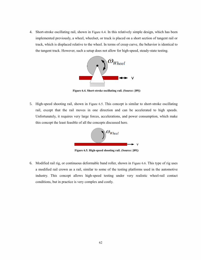
62

4. Short-stroke oscillating rail, shown in Figure 6.4. In this relatively simple design, which has been

implemented previously, a wheel, wheelset, or truck is placed on a short section of tangent rail or

track, which is displaced relative to the wheel. In terms of creep curve, the behavior is identical to

the tangent track. However, such a setup does not allow for high-speed, steady-state testing.

Figure 6.4. Short-stroke oscillating rail. (Source: [89])

5. High-speed shooting rail, shown in Figure 6.5. This concept is similar to short-stroke oscillating

rail, except that the rail moves in one direction and can be accelerated to high speeds.

Unfortunately, it requires very large forces, accelerations, and power consumption, which make

this concept the least feasible of all the concepts discussed here.

Figure 6.5. High-speed shooting rail. (Source: [89])

6. Modified rail rig, or continuous deformable band roller, shown in Figure 6.6. This type of rig uses

a modified rail crown as a rail, similar to some of the testing platforms used in the automotive

industry. This concept allows high-speed testing under very realistic wheel-rail contact

conditions, but in practice is very complex and costly.

63

Figure 6.6. Modified roller rig. (Source: [89])

The RTL report analyzed the above-discussed concepts and ranked them based on multiple

parameters (see the report for more information). The scores assigned to some of the concepts are shown

in Table 1.

Table 1: Roller rig concepts with top scores. (Source: [89])

The vertical plane design has the highest score in each category assuming the purpose of the roller rig

is the study of wheel/rail contact mechanics.

The question of the roller rig category (single wheel, single wheelset, or full truck) is primarily a

matter of cost and energy consumption. Although a full truck test rig would be desirable, a single

wheelset rig would be a good compromise between cost and performance, and therefore the rest of this

chapter will focus on this design.

64

6.2 Scaling

A single wheelset roller rig can be scaled according to any of the strategies described earlier in this

thesis. As the results in Chapter 5 show, INRETS’ strategy produces the same creep curves in a full-size

and in a scaled model. Therefore, if the roller rig’s primary purpose is the study of wheel-rail contact

mechanics and dynamics, INRETS’ strategy is preferable.

When length scaling factor 𝑓𝑙 is determined, all other scaling factors become its functions. Most

roller rigs in industry are either full-size or have 𝑓𝑙 between 2 and 5, although smaller-scale roller rigs

have been built, as discussed in the literature review (Chapter 2). Small scale rigs are less expensive to

build and operate than large-scale ones. Even more importantly, they allow attainment of high creep force

correction factors (𝑐𝑓11, 𝑐𝐹𝑥, etc.) for a relatively small-sized roller. However, the higher 𝑓𝑙 (or, in other

words, the smaller the scale) becomes, the higher the risk of encountering some effects that are

unaccounted for in this analysis. Furthermore, the smaller the scale, the larger the discrepancies between

the scaling of gravitational, elastic, and inertial forces (see Chapter 4 for the discussion of these

discrepancies). Finally, there is general distrust of small-scale testing setups in railroad industry.

Therefore, the decision regarding scaling should be made after carefully considering all of the above

factors.

6.3 Sensors

The sensors required for testing a single wheelset roller rig were outlined in a concept report prepared

earlier by the Railway Technologies Laboratory [89]. Note that the sensors listed in Table 2 were meant

for a full-scale roller rig. Depending on the scaling factor, not all of these sensors may be needed.

65

Table 2. Anticipated sensor requirements for a roller rig. (Source: [89])

LIDAR sensors are relatively new to the field and the literature search has not shown any roller rigs

that currently use or have used such sensors for velocity or displacement measurement. A more

conventional approach would involve the use of LVDT for displacement measurements and rotary

encoders for angular velocity measurements (for example, the roller rig described by Zhang et al. uses

grating encoders to measure rotational velocities and thus, indirectly, creepages [90]). High resolution,

accuracy, and precision are paramount for both velocity and displacement measurements because even a

minor displacement can cause a large change in contact patch radii ratio b/a, and a small change in

tangential velocity may cause a very large change in creepage. Recall that saturation creepages can be as

low as 0.5%. In other words, at tangent velocities of 10 m/s, the resolution of a velocity sensor should be

at least 10 to 20 times finer than 0.05 m/s, if we are to measure tangent velocities directly. For this reason,

it may be necessary to use multiple velocity sensors for different speeds. If rotary encoders are used to

measure angular velocities and tangent velocities are calculated from there, then 0.5% creepage at 10 m/s

tangent velocity (assuming both wheel and roller are 0.5m in diameter) corresponds to a difference of 0.1

rad/s in rotational velocities; again, the resolution must be at least 10-20 times finer than this number.

Accuracy may be improved by designing a setup in which a so-called reference shaft is linked to the

wheel and the roller in such a manner that its rotational velocity is the difference between the wheel and

roller’s rotational velocities (a similar approach was used by Matsumoto et al. [52]). Creepage would be

calculated by measuring the reference shaft’s angular velocity by either encoder or a LIDAR.

66

Note that even a small mistake in determining the wheel-roller contact point can lead to a major

mistake in determining creepage (see Eqs. 3.19 to 3.21, and 4.1 to 4.3). For example, a mistake of only

+/- 1mm in measuring the rolling radius of a wheel (0.5m nominal value) at the point of contact

corresponds to +/-0.002 mistake in creepage (recall that saturation creepage is on the order of 0.005 to

0.010).

It would be very desirable to measure the pressure distribution or at least a shape of the contact patch

in real time during rolling, but there is currently no method available to do so. Successful attempts have

been made to measure the pressure distribution in the contact patch using ultrasound, but this technology

is not yet advanced enough to conduct real-time measurements at high speed [91, 92]. As of today, the

only successful attempt to obtain such a measurement in real time was made by Poole, who placed an

array of 1-mm holes in a rail and pumped compressed air through the holes. Contact patch size and shape

were measured by observing the blockage of the holes by the wheel [93, 94].

6.4 Actuators and Constraints

Motors that control the rotation of the roller and of the axle are ultimately selected according to power

consumption, the calculation of which is described below. At a minimum, two motors are necessary for a

single-axle rig (one to power the rollers and one to power the wheels mounted on an axle) to achieve

steady state conditions. Three motors are needed to simulate a curve (one for each roller, and one for the

axle with wheels). Alternatively, one “main” and one “auxiliary” motor, combined with a differential gear,

can be used to power both rollers. We can either control the power supplied to the motors (thus

controlling the creep force indirectly), or their rotational velocities (thus controlling the creepage

indirectly). Typically, power is controlled and creepage becomes the dependent variable.

The transfer of power between the motors and the axles should be given very careful consideration,

considering the sensitivity of the rig to even the smallest variations in speed. Care must be taken to

control backlash in gears and possibly use constant velocity joints in place of universal joints.

If the purpose of the roller rig is the study of creep mechanics exclusively, then at first glance, no

compliant elements seem necessary. An axle or a bogie can be constrained in the longitudinal direction,

while being allowed to move freely in lateral, yaw, pitch, and roll directions (the latter two are only

relevant for a full bogie/truck rig) directions within a safe range. Hydraulic actuators can be used to apply

loads (either constant or variable) in vertical, longitudinal, and lateral directions. Yaw moment can be

applied by a pair of longitudinal hydraulic cylinders.

However, some yaw stiffness is necessary to prevent decrowning. The simplest way to achieve this is

to attach springs in parallel with the longitudinal hydraulic cylinders. These springs will provide both yaw

67

and longitudinal stiffness. If a more realistic behavior is desired (to simulate the suspension), springs can

be used in parallel with lateral and vertical cylinders as well.

Since creep mechanics are very sensitive to the rolling surfaces’ condition, a roller rig must be

designed to allow easy preconditioning (cleaning, wetting, possibly applying sand or top-of-rail friction

modifiers) of the surfaces. Ideally, there should also be an option to change the wheel and roller’s outer

parts (the tread and the crown) easily, without extensive disassembly.

6.5 Power Consumption

6.5.1 General Considerations

We will assume that the main source of power consumption is due to acceleration of rotating masses.

For a roller rig with a single wheelset, we can calculate the power required to achieve the needed

angular acceleration at a given angular velocity:

𝑃 = 𝑇𝜔 = 𝐼𝛼𝜔 6.1

If a roller rig is scaled, then rotational inertia, angular acceleration, and angular velocity will be scaled

as well, and so will power. Eq. 6.26 is then transformed into:

𝑃 = (𝐼0𝛼0𝜔0)(𝑓𝐼𝑓𝛼𝑓𝜔)−1 6.2

Here, 𝑋0 designates a value of a given quality for a full-size wheelset, and 𝑓𝑋 is the scaling factor for

this quality.

These formulas are meant for the wheelset itself; the roller is not scaled in the strict sense, as its

rolling radius can be chosen independently of other scaling parameters. Therefore, Eq. 6.1 is useful for

either wheelset or roller, while Eq. 6.2 applies to wheelset only.

These equations also allow us to predict the required power dissipation capacity when braking, as

opposed to acceleration, is simulated.

We will determine the appropriate scaling factors for the three scaling strategies discussed earlier

(Jaschinski’s, Pascal’s, and Iwnicki’s) from the factors given in Bosso et al. and Allen’s works [6, 87].

6.5.2 Jaschinski’s (DLR) Scaling Strategy with Density SF of 1

The SF for velocity, rotational inertia, and linear acceleration in terms of length SF are given as:

𝑓𝑉 = √𝑓𝑙 6.3

68

𝑓𝐼 = 𝑓𝑙5 6.4

𝑓𝑎 = 1

6.5

From here, we derive SF for angular velocity and angular acceleration:

𝑓𝜔 =𝑓𝑉𝑓𝑙

=√𝑓𝑙𝑓𝑙

= 𝑓𝑙−0.5 6.6

𝑓𝛼 =𝑓𝑎𝑓𝑙

= 𝑓𝑙−1 6.7

These, combined with Eq. 6.2, give us:

𝑃 = (𝐼0𝛼0𝜔0)(𝑓𝐼𝑓𝛼𝑓𝜔)−1 = (𝐼0𝛼0𝜔0)(𝑓𝑙

5𝑓𝑙−1𝑓𝑙

−0.5)−1

= (𝐼0𝛼0𝜔0)𝑓𝑙−3.5

6.8

6.5.3 Jaschinski’s Strategy with a Non-unity Density SF

In this case SF for angular velocity and acceleration do not change, but SF for rotational inertia does:

𝑓𝐼 = 𝑓𝜌𝑓𝑙5 6.9

Therefore, the equation for power changes slightly:

𝑃 = (𝐼0𝛼0𝜔0)(𝑓𝐼𝑓𝛼𝑓𝜔)−1 = (𝐼0𝛼0𝜔0)(𝑓𝜌𝑓𝑙5𝑓𝑙

−1𝑓𝑙−0.5)

−1

= (𝐼0𝛼0𝜔0)𝑓𝑙−3.5𝑓𝜌

−1 6.10

6.5.4 Pascal’s (INRETS) Scaling Strategy

The SF for velocity, rotational inertia, and acceleration are given as:

𝑓𝑉 = 1 6.11

𝑓𝐼 = 𝑓𝑙5 6.12

𝑓𝑎 = 𝑓𝑙−1 6.13

69

Other SF are derived from here:


=1

𝑓𝑙= 𝑓𝑙

−1 6.14

𝑓𝛼 =

𝑓𝑎𝑓𝑙

=𝑓𝑙

−1

𝑓𝑙= 𝑓𝑙

−2

6.15

And the power equation in this case is:

𝑃 = (𝐼0𝛼0𝜔0)(𝑓𝐼𝑓𝛼𝑓𝜔)−1 = (𝐼0𝛼0𝜔0)(𝑓𝑙5𝑓𝑙

−2𝑓𝑙−1)−1

= (𝐼0𝛼0𝜔0)𝑓𝑙−2

6.16

6.5.5 Iwnicki’s (MMU) Scaling Strategy

Given are the scaling factors:

𝑓𝑉 = 𝑓𝑙 6.17

𝑓𝐼 = 𝑓𝑙5 6.18

𝑓𝑎 = 𝑓𝑙 6.19

From here we derive other SF:


=𝑓𝑙𝑓𝑙

= 1 6.20

𝑓𝛼 =𝑓𝑎𝑓𝑙

=𝑓𝑙𝑓𝑙

= 1 6.21

And, finally, the equation for power:

𝑃 = (𝐼0𝛼0𝜔0)(𝑓𝐼𝑓𝛼𝑓𝜔)−1 = (𝐼0𝛼0𝜔0)𝑓𝑙−5 6.22

6.5.6 Modified Power Equations

It may be useful to modify the power equations to express power consumption in terms of wheel

rolling radius, linear velocity, and linear acceleration (of a full-scale rig). These parameters relate more

70

closely to the design objectives, which may include simulating specific speeds and accelerations. We then

easily obtain:

Jaschinski (density SF=1):

𝑃 = 𝐼𝛼𝜔 = 𝐼 𝑎

𝑟

𝑣

𝑟=

𝐼0𝑎0𝑣0

𝑟02 (𝑓𝐼𝑓𝑎𝑓𝑉𝑓𝑙

−2)−1

=𝐼0𝑎0𝑣0

𝑟02 (𝑓𝑙

5√𝑓𝑙𝑓𝑙−2)

−1=

𝐼0𝑎0𝑣0

𝑟02 𝑓𝑙

−3.5

6.23

Jaschinski (other density SF):


𝑟

𝑣

𝑟=

𝐼0𝑎0𝑣0


−2)−1

=𝐼0𝑎0𝑣0

𝑟02 (𝑓𝜌𝑓𝑙

5√𝑓𝑙𝑓𝑙−2)

−1

=𝐼0𝑎0𝑣0

𝑟02 𝑓𝜌

−1𝑓𝑙−3.5

6.24

Pascal:


𝑟

𝑣

𝑟=

𝐼0𝑎0𝑣0


−2)−1

=𝐼0𝑎0𝑣0

𝑟02 (𝑓𝑙

5𝑓𝑙−1𝑓𝑙

−2)−1

=𝐼0𝑎0𝑣0

𝑟02 𝑓𝑙

−2

6.25

Iwnicki:


𝑟

𝑣

𝑟=

𝐼0𝑎0𝑣0


−2)−1

=𝐼0𝑎0𝑣0

𝑟02 (𝑓𝑙

5𝑓𝑙𝑓𝑙𝑓𝑙−2)

−1=

𝐼0𝑎0𝑣0

𝑟02 𝑓𝑙

−5

6.26

These equations should help a researcher in choosing a cost-effective scaling strategy, as well as in

specifying the actuators for a roller rig.

71

6.6 Data Processing

If a roller rig is used to verify Kalker’s coefficients (c11, c22, etc.), one way to extrapolate its data to

tangent track would be the following algorithm (for simplicity, here we will consider pure longitudinal

creepage).

The user applies the needed vertical load to the wheelset on a roller rig. He then runs the roller rig at

different creepages and measures the resulting creep forces. As long as the creepages are within the linear

range (i.e. in the range where Kalker’s linear theory applies), the resulting data points should make a line

whose slope corresponds to the f11 coefficient. Knowing this slope and the shape of the contact patch

(either by direct measurement, ex. contact film, or from Hertzian theory), the user then calculates

Kalker’s coefficient c11. This becomes a datapoint in a “c11 vs. b/a” curve. By repeating this experiment

for different wheel or rail curvatures (which can be achieved either by using different wheels or by

changing roller cant such that the rail’s transverse curvature and, consequently, b/a ratio, changes), the

user then obtains an empirical relationship between contact patch shape and creepage coefficient. This

relationship can be compared against the existing tables.

Once the relationship between b/a and c11 is established, it can be used to find the correction factors

for creep forces without relying on existing theoretical data (after all, the purpose of the experiment

would be to verify it).

It is important to remember that a number of approximations (such as the polynomial fits for Kalker’s

coefficients) were used in order to obtain explicit, closed-loop relationships. Therefore, depending on the

precision required, it may be very desirable, once an optimal scaling strategy and scaling factors are

selected using the relationships above, to use more accurate methods, such as table interpolation, to obtain

more accurate values for correction and transformation factors.

72

7 Summary and Conclusions

7.1 Summary

This thesis has quantified the differences between the tangent track and a roller rig in terms of their

creep forces vs. creepage.

First, an overview of existing creep models used in rail vehicle dynamics was given, along with an

overview of some of the roller rigs used in wheel-rail contact mechanics research. Then, two of the

models described in the review (Kalker’s linear theory and Johnson and Vermeulen’s theory) were used to

compare creep curves on a roller rig to those on a tangent track.

The relationship between the slope of Kalker’s creep curve (representing creep force per unit

creepage) on a roller rig to that on a tangent track was derived. Based on Kalker’s linear theory of tangent

contact and Hertzian theory of normal contact, correction factors for creep force per unit creepage were

derived. A similar analysis was conducted using Johnson and Vermeulen’s theory.

Various scaling strategies for roller rigs were compared. Scaling factors for creep forces were derived

using both Kalker’s and Johnson and Vermeulen’s theories. Transformation factors, which are functions of

scaling factors and correction factors, were derived to compare roller rigs and tangent tracks of various

scales.

A case study was given, in which correction, scaling, and transformation factors were shown for

specific wheel-rail and wheel-roller configurations to illustrate the relationships derived earlier in this

thesis. A number of articles quantifying the roller rig vs. tangent track differences were reviewed, and a

comparison of their results with the results of this thesis was given.

General recommendations on design and scaling of a roller rig were provided. Special attention was

given to the measurement of creepage.

7.2 Conclusions

The main conclusions from this study are:

1. Kalker’s linear theory is easier to use in terms of quantifying the differences between a tangent

track and roller rig; however, it only applies at small creepages.

2. For the same purposes, Johnson and Vermeulen’s theory is more difficult to use than Kalker’s, but

it is likely the most convenient among the non-linear theories.

73

3. Closed-form, deterministic relationships exist between normalized creep force on a tangent track

vs. a roller rig. If the track and the rig are of the same scale, these relationships can be described

in terms of correction factors. For different scales, transformation factors can be derived.

4. If the diameter of the roller is the design-limiting factor for a roller rig, then the larger the length

scaling factor, the closer the roller rig represents a tangent track in terms of creep force correction

factors; i.e., the smaller the wheelset is, the more closely such a roller rig represents a tangent

track because the roller’s diameter is much larger than the wheel’s diameter.

5. For Kalker’s theory, creep force correction factors are independent of wheel load and scaling.

They are functions of contact patch aspect ratio, which is a function of the wheel and roller’s

relative surface curvatures at the point of contact.

6. The correction factors for Kalker’s linear theory are close to those predicted by other authors.

7. INRETS’ scaling strategy ensures that correction factors for normalized creep forces are scale-

independent. This is true both under Kalker’s and Johnson and Vermeulen’s theories. Therefore,

this strategy should be used when designing a scaled roller rig for the purpose of studying wheel-

rail contact mechanics.

8. At small creepages, the difference between a roller rig and a tangent track in terms of normalized

creep forces is the largest. As creepage increases, the correction factors approach 1, i.e. the roller

rig and tangent track behave similarly.

9. When designing a roller rig for studying creep mechanics, it is very desirable to have a way of

measuring the contact patch dimensions in real time. This could potentially be done using

ultrasound, but this technology is not yet sufficiently developed.

10. It is crucial to measure creepages and the location of the wheel-rail contact point with extreme

accuracy in order to extract the creep data from a roller rig.

7.3 Future Work

The future work on the topic of this thesis should include:

1. Case studies involving realistic wheel and rail profiles (such as those in Figure 2.2).

2. Studies involving non-linear creep theories other than Johnson and Vermeulen (ex. FASTSIM).

3. A more in-depth analysis of scaling strategies other than INRETS’.

4. A detailed design of a roller rig based on the conclusions of this thesis.

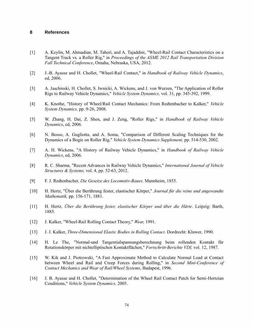
74

8 References

[1] A. Keylin, M. Ahmadian, M. Taheri, and A. Tajaddini, "Wheel-Rail Contact Characteristics on a

Tangent Track vs. a Roller Rig," in Proceedings of the ASME 2012 Rail Transportation Division

Fall Technical Conference, Omaha, Nebraska, USA, 2012.

[2] J.-B. Ayasse and H. Chollet, "Wheel-Rail Contact," in Handbook of Railway Vehicle Dynamics,

ed, 2006.

[3] A. Jaschinski, H. Chollet, S. Iwnicki, A. Wickens, and J. von Wurzen, "The Application of Roller

Rigs to Railway Vehicle Dynamics," Vehicle System Dynamics, vol. 31, pp. 345-392, 1999.

[4] K. Knothe, "History of Wheel/Rail Contact Mechanics: From Redtenbacher to Kalker," Vehicle

System Dynamics, pp. 9-26, 2008.

[5] W. Zhang, H. Dai, Z. Shen, and J. Zeng, "Roller Rigs," in Handbook of Railway Vehicle

Dynamics, ed, 2006.

[6] N. Bosso, A. Gugliotta, and A. Soma, "Comparison of Different Scaling Techniques for the

Dynamics of a Bogie on Roller Rig," Vehicle System Dynamics Supplement, pp. 514-530, 2002.

[7] A. H. Wickens, "A History of Railway Vehicle Dynamics," in Handbook of Railway Vehicle

Dynamics, ed, 2006.

[8] R. C. Sharma, "Recent Advances in Railway Vehicle Dynamics," International Journal of Vehicle

Structures & Systems, vol. 4, pp. 52-63, 2012.

[9] F. J. Redtenbacher, Die Gesetze des Locomotiv-Baues. Mannheim, 1855.

[10] H. Hertz, "Über die Berührung fester, elastischer Körper," Journal für die reine und angewandte

Mathematik, pp. 156-171, 1881.

[11] H. Hertz, Über die Berührung fester, elastischer Körper und über die Härte. Leipzig: Barth,

1885.

[12] J. Kalker, "Wheel-Rail Rolling Contact Theory," Wear, 1991.

[13] J. J. Kalker, Three-Dimensional Elastic Bodies in Rolling Contact. Dordrecht: Kluwer, 1990.

[14] H. Le The, "Normal-und Tangentialspannungsberechnung beim rollenden Kontakt für

Rotationskörper mit nichtelliptischen Kontaktflächen," Fortschritt-Berichte VDI, vol. 12, 1987.

[15] W. Kik and J. Piotrowski, "A Fast Approximate Method to Calculate Normal Load at Contact

between Wheel and Rail and Creep Forces during Rolling," in Second Mini-Conference of

Contact Mechanics and Wear of Rail/Wheel Systems, Budapest, 1996.

[16] J. B. Ayasse and H. Chollet, "Determination of the Wheel Rail Contact Patch for Semi-Hertzian

Conditions," Vehicle System Dynamics, 2005.

75

[17] J. Piotrowski and H. Chollet, "Wheel-Rail Contact Models for Vehicle System Dynamics

including Multi-point Contact," Vehicle System Dynamics, 2005.

[18] V. Yazykov, D. Pogorelov, and G. Mikhalchenko, "Railway Vehicle Simulation Using Non-

elliptical Wheel-Rail Contact Model," in XXI ICTAM Proceedings, Warsaw, Poland, 2004.

[19] K. Knothe and H. Le The, "A Contribution to the Calculation of the Contact Stress Distribution

Between Two Elastic Bodies of Revolution with Non-elliptical Contact Area," Computers &

Structures, vol. 18, 1984.

[20] R. Enblom and M. Berg, "Impact of Non-elliptic Contact Modelling in Wheel Wear Simulation,"

Wear, vol. 265, 2008.

[21] C. Linder and H. Brauchi, "Prediction of Wheel Wear," in Proceedings of 2nd Mini Conference on

Contact Mechanics and Wear of Rail/Wheel Systems, Budapest, 1996.

[22] A. Alonso and J. G. Giménez, "A New Method for the Solution of the Normal Contact Problem in

the Dynamic Simulation of Railway Vehicles," Vehicle System Dynamics, 2005.

[23] T. Telliskivi, "Simulation of Wear in a Rolling-Sliding Contact by a Semi-Winkler Model and

Archard's Wear Law," Wear, 2004.

[24] U. Olofsson and R. Lewis, "Tribology of the Wheel-Rail Contact," in Handbook of Railway

Vehicle Dynamics, S. Iwnicki, Ed., ed, 2006.

[25] F. W. Carter, "The Electric Locomotive," Proceedings of the Institute of Civil Engineers, 1916.

[26] C. Boedecker, Die Wirkungen zwischen Rad und Schiene und ihre Einflüsse auf den Lauf und den

Bewegungswiderstand der Fahrzeuge in den Eisenbahnzügen. Hannover: Hahn, 1887.

[27] O. Reynolds, "On the Efficiency of Belts or Straps as Communicators of Work," The Engineer,

1874.

[28] F. Carter, "On the Action of a Locomotive Driving Wheel," Proceedings of the Royal Society of

London. Series A, Containing Papers of a Mathematical and Physical Character., vol. 112, 1926.

[29] A. E. H. Love, Mathematical Theory of Elasticity, 2nd Edition, 1906.

[30] H. Fromm, "Berechnung des Schlupfes beim Rollen deformierbarer Scheiben," Zeitschrift fur

Angewandte Mathmatik and Mechanik, 1926.

[31] H. Poritsky, "Stresses and Deflections of Cylindrical Bodies in Contact with Application to

Contact of Gears and of Locomotive Wheels," Journal of Applied Mechanics, pp. 191-201, 1950.

[32] K. L. Johnson, "The Effect of Tangential Contact Force upon the Rolling Motion of an Elastic

Sphere on a Plane," Transactions of ASME, Journal of Applied Mechanics, pp. 339-346, 1958.

[33] C. Cattaneo, "Sul Contatto di due Corpi Elastici," Accademia de Lincei, Rendi conti, vol. 27,

1938.

[34] P. J. Vermeulen and K. L. Johnson, "Contact of Nonspherical Elastic Bodies Transmitting

Tangential Forces," Journal of Applied Mechanics, 1964.

76

[35] K. L. Johnson, "The Effect of Spin upon a Rolling Motion of an Elastic Sphere upon a Plane,"

Transactions of ASME, Journal of Applied Mechanics, pp. 332-338, 1958.

[36] D. J. Haines and E. Ollerton, "Contact Stress Distributions on Elliptical Contact Surfaces

Subjected to Radial and Tangential Forces," Proceedings of the Institution of Mechanical

Engineers, vol. 177, 1963.

[37] A. D. De Pater, "On the Reciprocal Pressure between Two Elastic Bodies," in Proceedings of

Symposium on Rolling Contact Phenomena, Amsterdam, Netherlands, 1962.

[38] J. J. Kalker, "The Transmission of Force and Couple Between Two Elastically Similar Rolling

Spheres," in Proceedings Koninklijke Nederlandse Akademie van Wetenschappen, Amsterdam,

Netherlands, 1964.

[39] Z. Y. Shen, J. K. Hendrick, and J. A. Elkins, "A Comparison of Alternative Creep-Force Models

for Rail Vehicle Dynamic Analysis," in Proceedings of 8th IAVSD Symposium, Campridge, MA,

United States, 1984.

[40] T. Ohyama, "Some Problems of the Fundamental Adhesion at Higher Speeds," Quarterly Report

of RTRI, vol. 14, 1973.

[41] F. Bucher, The Contact between Micro-Rough Rails and Wheels. Berlin: Logos Verlag, 2002.

[42] W. Bucher, A. I. Dmitriev, M. Ertz, K. Knothe, V. L. Popov, S. G. Psakhie, et al., "Multiscale

Simulation of Dry Friction in Wheel/Rail Contact," Wear, 2004.

[43] W. Lang and G. Roth, "Optimale Kraftschlußausnutzung bei Hochleistungs-

Schienenfahrzeugen.," Eisenbahntechnische Rundschau, 1993.

[44] B. R. Meyer, "High-adhesion Locomotives with Controlled Creep," Institution of Mechanical

Engineers, vol. C81/87, pp. 209-218, 1987.

[45] O. Polach, "Creep Forces in Simulations of Traction Vehicles Running on Adhesion Limit," Wear,

pp. 992-1000, 2005.

[46] E. M., "Temperatur, Materialbeanspruchung und Kraftschluss im Rad-Schiene-Kontakt,"

Fortschritt-Berichte VDI, vol. 549, 2004.

[47] M. Spiryagin, K. S. Lee, H. H. Yoo, O. Kashura, and O. Kostyukevich, "Modeling of Adhesion

for Railway Vehicles," Journal of Adhesion Science and Technology, vol. 22, pp. 1017-1034,

2008.

[48] H. Yamazaki, M. Nagai, and T. Kamada, "A Study of Adhesion Force Model for Wheel Slip

Prevention Control," JSME International Journal, Series C: Mechanical Systems, Machine

Elements and Manufacturing, vol. 47, pp. 496-501, 2004.

[49] S. H. Park, J. S. Kim, J. J. Choi, and H. Yamazaki, "Modeling and Control of Adhesion Force in

Railway Rolling Stocks," IEEE Control Systems Magazine, vol. 28, pp. 44-58, 2008.

77

[50] M. Malvezzi, B. Allotta, and L. Pugi, "Feasibility of Degraded Adhesion Tests in a Locomotive

Roller Rig," Proceedings of the Institution of Mechanical Engineers. Part F, Journal of Rail and

Rapid Transit, vol. 222, 2008.

[51] R. Conti, E. Meli, L. Pugi, M. Malvezzi, F. Bartolini, B. Allotta, et al., "A Numerical Model of a

HIL Scaled Roller Rig for Simulation of Wheel–Rail Degraded Adhesion Condition," Vehicle

System Dynamics, vol. 50, pp. 775-804, 2012.

[52] K. Matsumoto, Y. Suda, H. Komine, T. Nakai, M. Tomeoka, K. Shimizu, et al., "Proposal of

Wheel/Rail Contact Model for Friction Control," Journal of Mechanical Science and Technology,

vol. 19, pp. 437-443, 2005.

[53] L. Pugi, A. Ridolfi, M. Malzezzi, F. Cangioli, and A. Rindi, "Three Dimensional Modelling of

Wheel–Rail Degraded Adhesion Conditions," in 22nd International Symposium on Dynamics of

Vehicles on Roads and Tracks, Manchester, UK, 2011.

[54] D. R. Carling, "Locomotive Testing Stations," Transactions of the Newcomen Society, vol. 45,

1972.

[55] T. Matsudaira, "Shimmy of Axle with Pair of Wheels (in Japanese)," Journal of Railway

Engineering Research, pp. 16-26, November 1952.

[56] T. Matsudaira, N. Matsui, S. Arai, and K. Yokose, "Problems on Hunting of Railway Vehicle on

Test Stand," Transactions of ASME Journal of Engineering in Industry, vol. 91 ser. B, pp. 879-

885, 1969.

[57] A. H. Wickens and A. O. Gilchrist, "Railway Vehicle Dynamics - The Emergence of a Practical

Theory ", ed: CEI MacRobert Award Lecture, 1977.

[58] L. M. Sweet, J. A. Sivak, and W. F. Putman, "Non-linear Wheelset Forces in Flange Contact,"

Journal of Dynamics Systems, Measurement and Control, vol. 101, pp. 238-255, 1979.

[59] L. M. Sweet, A. Karmel, and S. R. Fairley, "Derailment Mechanics and Safety Criteria for

Complete Railway Vehicle Trucks," in Proceedings of 7th IAVSD Symposium, Cambridge, UK,

1981.

[60] M. Cox and H. Nicolin, "Untersuchung des Schwingungsverhaltens von Schienenfahrzeugen mit

Hilfe des Modellprufstands am Institut fur Fordertechnik und Schienenfahrzeuge der RWTH

Aachen," Leichtbau der Verkehrsfahrzeuge, vol. 23, pp. 91-95, 1979.

[61] D. Lubke, M. Mittermaier, L. Pfaffl, and F. Zollner, "Ein Rollprufstand zur Erforschung der

Rad/Schiene-Technik," ZEV Glasers Annalen, vol. 100, pp. 295-305, 1976.

[62] K. Althammer and L. Pfaffl, "Versuchsanlage Rollprufstand," Eisenbahntechnische Rundschau,

vol. 25, pp. 663-676, 1976.

[63] K. Althammer, "Planung, Bau und Betrieb des Rollprufstandes fur das RadrSchiene-

Forschungsprogramm.," ZEV Glasers Annalen, vol. 101, pp. 312-323, 1977.

[64] H. Hahn and G. Sigl, "Simulation und experimentelle Verifikation des Radr/Schiene-

Rollprufstands.," Ingenieur Archiv, vol. 57, pp. 329-348, 1987.

78

[65] R. H. Fries, "Estimation of Transit Rail Vehicle Parameter from Roller Rig Tests; Ph.D.

Dissertation," ed: Arizona State University, 1983.

[66] R. H. Fries, Personal communication with author ed, 2012.

[67] M. Jochim, "Konstruktion eines Versuchsdrehgestells," ed. Oberpfaffenhofen: Term study,

Lehrstuhl B fur Mechanik, 1984.

[68] M. Jochim, "Analyse der Dynamik eines Schienenfahrzeuges," ed. Oberpfaffenhofen: Diploma

thesis, Lehrstuhl B fur Mechanik, TU-Munchen and DLR, 1987.

[69] A. Jaschinski, "On the Application of Similarity Laws to a Scaled Railway Bogie Model," ed.

Oberpfaffenhofen: Dissertation. TU-Delft, 1990.

[70] H. Chollet, "Essais en Similitude a l’Echelle 1/4 de Bogies de Wagons de la Famille Y25,"

INRETS-Report No. 781988.

[71] H. Chollet, "Etude en Similitude Mechanique des Efforts Tangents au Contact Roue-Rail," ed:

Dissertation, Universite Paris, 1991.

[72] S. D. Iwnicki and Z. Y. Shen, "Collaborative railway roller rig project," in Proceedings of SEFI

World Conference on Engineering Education, Portsmouth, 1992.

[73] S. D. Iwnicki and A. H. Wickens, "Validation of a MATLAB Railway Vehicle Simulation Using a

Scale Roller Rig," Vehicle System Dynamics, vol. 30, pp. 257-270, 1998.

[74] B. Alotta, L. Pugi, M. Malvezzi, F. Bartolini, and F. Cangioli, "A Scaled Roller Test Rig for High-

Speed Vehicles," Vehicle System Dynamics, vol. 48 (Supplement), pp. 3-18, 2010.

[75] R. Stock, D. Eadie, D. Elvidge, and K. Oldknow, "Influencing Rolling Contact Fatigue through

Top of Rail Friction Modifier Application – a Full Scale Wheel–Rail Test Rig Study," Wear, vol.

271, pp. 134-142, 2011.

[76] Q. Y. Liu, B. Zhang, and Z. R. Zhou, "An Experimental Study of Rail Corrugation," Wear, vol.

255, pp. 1121-1126, 2005.

[77] W. J. Wang, H. F. Zhang, H. Y. Wang, Q. Y. Liu, and M. H. Zhu, "Study on the Adhesion

Behavior of Wheel/Rail under Oil, Water and Sanding Conditions," Wear, vol. 271, pp. 2693-

2698, 2011.

[78] Y. Michitsuji and Y. Suda, "Running Performance of Power-Steering Railway Bogie with

Independently Rotating Wheels," Vehicle System Dynamics, vol. 44 (Supplement), pp. 71-82,

2006.

[79] Y. Suda, W. Wang, M. Nishina, S. Lin, and Y. Michitsuji, "Self-Steering Ability of the Proposed

New Concept of Independently Rotating Wheels Using Inverse Tread Conicity," Vehicle System

Dynamics, vol. 44 (Supplement), pp. 71-82, 2006.

[80] M.-S. Kim and H.-M. Hur, "Application of Braking/Traction Control Systems to the Scaled

Active Steering Testbed in the Railway Vehicle," WSEAS Transactions on Systems and Control,

vol. 4, pp. 296-305, 2009.

79

[81] M.-S. Kim, J.-H. Park, and W.-Y. You, "Construction of Active Steering System of the Scaled

Railway Vehicle," International Journal of Systems Applications, Engineering & Development,

vol. 2, pp. 217-226, 2008.

[82] D. Thompson, Railway Noise and Vibration: Mechanisms, Modelling and Means of Control:

Elsevier, 2009.

[83] H. W. Lee, "A Polynomial Chaos Approach for Stochastic Modeling of Dynamic Wheel-Rail

Friction," ed: PhD Thesis, Virginia Tech, 2010.

[84] K. E. Zaazaa and A. L. Schwab, "Review of Joost Kalker's Wheel-Rail Contact Theories and

Their Implementation in Multibody Codes," in Proceedings of the ASME 2009 International

Design Engineering Technical Conferences & Computer and Information in Engineering

Conference, San Diego, California, USA, 2009.

[85] N. Bosso, A. Gugliotta, and A. Soma, "Dynamic Behavior of a Railway Wheelset on a Roller Rig

versus Tangent Track," Shock and Vibration, pp. 467-492, 2004.

[86] R. Dukkipati, "Dynamics of a Wheelset of Roller Rig," Vehicle System Dynamics, vol. 30, pp.

409-430, 1998.

[87] P. D. Allen, "Scale Testing," in Handbook of Railway Vehicle Dynamics, ed, 2006.

[88] F. Blader, "Fundamental Differences between The RDU and an Ideal Track in Determining

Vehicle Lateral Dynamics," Blader Engineering Limited.

[89] "Evaluation of Wheel/Rail Contact Mechanics: Concepts Report," Railway Technologies

Laboratory, Blacksburg, VA, 2011.

[90] W. Zhang, J. Chen, X. Wu, and X. Jin, "Wheel/Rail Adhesion and Analysis by Using Full Scale

Roller rig," Wear, vol. 253, pp. 82-88, 2002.

[91] M. Pau, F. Aymerich, and F. Ginesu, "Distribution of Contact Pressure in Wheel-Rail Contact,"

Wear, vol. 253, pp. 265-274, 2002.

[92] M. Pau, B. Leban, and A. Baldi, "Simultaneous Subsurface Defect Detection and Contact

Parameter Assessment in a Wheel–Rail System," Wear, vol. 265, pp. 1837-1847, 2008.

[93] W. Poole, "The Measurement of the Contact Area between Opaque Objects under Static and

Dynamic Rolling Conditions," in Proceedings of Conference on Contact Mechanics and Wear of

Rail/Wheel Systems II, 1986.

[94] M. B. Marshall, R. Lewis, and R. S. Dwyer-Joyce, "Experimental Characterization of Wheel-Rail

Contact Patch Evolution," Journal of Tribology, vol. 128, pp. 493-504, 2006.

analytical evaluation of the accuracy of … 2.8. force-creep curves for various rail and wheel...

Documents