analytical assessment of an irregular rc full scale 3d

Analytical Assessment

of an Irregular RC Full Scale 3D Test Structure

by

Seong-Hoon Jeong and Amr S. Elnashai

Department of Civil and Environmental Engineering University of Illinois at Urbana-Champaign

Urbana, Illinois

March 2004

This research is supported by the Mid-America Earthquake Center under National Science Foundation Grant EEC-9701785

Mid-America Earthquake CenterHeadquartered at the University of Illinois at Urbana-Champaign

Amr S. Elnashai, Ph.D., Director

ACKNOWLEDGEMENT

This report is a deliverable of project CM-4: Structural Retrofit Strategies, part of the Mid-America Earthquake Center Core Research Program under the Thrust Area Consequence Minimization, coordinated by Professors Barry Goodno and Steven French (Georgia Institute of Technology). The authors have benefited from discussions with members of the European research network Seismic Performance Assessment and Rehabilitation (SPEAR) under which the structure described in the report was tested at full scale at the European Laboratory for Structural Assessment (ELSA) of the Joint Research Center (JRC), Ispra, Italy. Thanks are due to Professors Paolo E. Pinto, Michael N. Fardis, Gian Michele Calvi, Drs. Eduardo C. Carvalho, Paolo Negro, Mr. Francisco J. Molina and Miss Elena Mola. The cooperation of members of the ELSA is gratefully acknowledged. This work was supported primarily by the Mid-America Earthquake Center through the Earthquake Engineering Research Centers Program of the National Science Foundation under NSF Award No. EEC-9701785. Any opinions, findings and conclusions or recommendations expressed in this material are those of the authors and do not necessarily reflect those of the National Science Foundation.

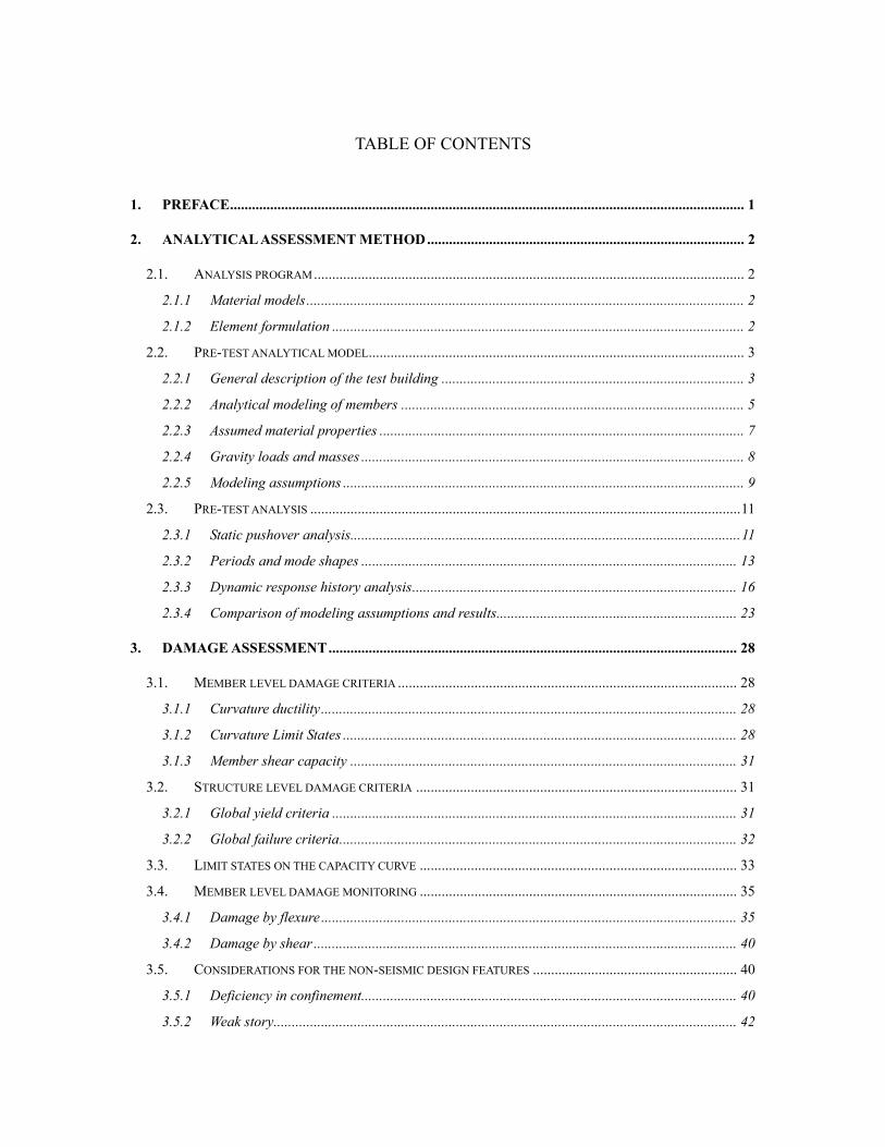
TABLE OF CONTENTS

1. PREFACE............................................................................................................................................. 1

2. ANALYTICAL ASSESSMENT METHOD....................................................................................... 2

2.1. ANALYSIS PROGRAM...................................................................................................................... 2 2.1.1 Material models........................................................................................................................ 2 2.1.2 Element formulation ................................................................................................................. 2

2.2. PRE-TEST ANALYTICAL MODEL....................................................................................................... 3 2.2.1 General description of the test building ................................................................................... 3 2.2.2 Analytical modeling of members .............................................................................................. 5 2.2.3 Assumed material properties .................................................................................................... 7 2.2.4 Gravity loads and masses ......................................................................................................... 8 2.2.5 Modeling assumptions .............................................................................................................. 9

2.3. PRE-TEST ANALYSIS ......................................................................................................................11 2.3.1 Static pushover analysis...........................................................................................................11 2.3.2 Periods and mode shapes ....................................................................................................... 13 2.3.3 Dynamic response history analysis......................................................................................... 16 2.3.4 Comparison of modeling assumptions and results.................................................................. 23

3. DAMAGE ASSESSMENT................................................................................................................ 28

3.1. MEMBER LEVEL DAMAGE CRITERIA ............................................................................................. 28 3.1.1 Curvature ductility.................................................................................................................. 28 3.1.2 Curvature Limit States ............................................................................................................ 28 3.1.3 Member shear capacity .......................................................................................................... 31

3.2. STRUCTURE LEVEL DAMAGE CRITERIA ........................................................................................ 31 3.2.1 Global yield criteria ............................................................................................................... 31 3.2.2 Global failure criteria............................................................................................................. 32

3.3. LIMIT STATES ON THE CAPACITY CURVE ....................................................................................... 33 3.4. MEMBER LEVEL DAMAGE MONITORING ....................................................................................... 35

3.4.1 Damage by flexure.................................................................................................................. 35 3.4.2 Damage by shear .................................................................................................................... 40

3.5. CONSIDERATIONS FOR THE NON-SEISMIC DESIGN FEATURES ........................................................ 40 3.5.1 Deficiency in confinement....................................................................................................... 40 3.5.2 Weak story............................................................................................................................... 42

3.5.3 Torsion .................................................................................................................................... 42 3.5.4 Bidirectional loading .............................................................................................................. 44

4. EARTHQUAKE SCENARIO FOR THE TEST............................................................................. 45

4.1. METHODOLOGY AND CRITERIA .................................................................................................... 45 4.1.1 Ground motion records ........................................................................................................... 45 4.1.2 Interstory drift as a damage index.......................................................................................... 46 4.1.3 Selection of ground motion ..................................................................................................... 48 4.1.4 Intensity of ground motion for the test .................................................................................... 50 4.1.5 Direction of application of ground motion ............................................................................. 53

4.2. BEHAVIOR AND DAMAGE ESTIMATIOIN......................................................................................... 55 4.2.1 Damage expectation and selection of a scenario ................................................................... 55 4.2.2 Displacement information for the test setup ........................................................................... 58

5. REFINEMENT OF THE PRE-TEST ANALYTICAL MODELING............................................ 59

5.1. MATERIAL PROPERTIES UPDATE ................................................................................................... 59 5.2. RIGID DIAPHRAGM MODELING OF FLOOR SLABS........................................................................... 60 5.3. MODELING OF BEAM-COLUMN CONNECTIONS.............................................................................. 62

5.3.1 Shear deformation modeling of RC beam-column connections.............................................. 62 5.3.2 Response of beam-column connections .................................................................................. 67

5.4. COMPARISON OF RESPONSES OF PRE-TEST ANALYTICAL MODELS ................................................. 70

6. DEPLOYMENT OF ANALYTICAL MODELS FOR TEST EXECUTION............................. 71

6.1. PRE-TEST CONDITION ASSESSMENT OF THE STRUCTURE............................................................... 71 6.1.1 Cause of damage during transportation................................................................................. 71 6.1.2 Investigation of cracks............................................................................................................ 73 6.1.3 Numerical simulation for the condition assessment of the test structure................................ 74

6.2. DETERMINATION OF ACTUATOR MOVEMENT ................................................................................ 80 6.3. GRAVITY LOAD DISTRIBUTION FOR THE TEST ............................................................................... 82

7. EXPERIMENTAL RESULTS AND COMPARISONS................................................................... 84

7.1. OVERVIEW OF THE FULL-SCALE PSEUDO-DYNAMIC TEST ............................................................. 84 7.2. COMPARISON OF EXPERIMENTAL RESULTS AND PRE-TEST ANALYSIS ............................................ 86

7.2.1 Damage description................................................................................................................ 86 7.2.2 Comparison and discussion.................................................................................................... 88

8. CONCLUSION .................................................................................................................................. 94

9. REFERENCES .................................................................................................................................. 97

Appendix A. Curvature limit states of members ............................................................................102 Appendix B. Global yield limit states............................................................................................106 Appendix C. Elastic response spectra of records for the SPEAR test............................................107 Appendix D. Angle of torsion time histories under Montenegro 1979 (Herceg Novi)

with various intensities and directions .....................................................................110 Appendix E. Interstory drift time histories under Montenegro 1979 (Herceg Novi)

with various intensities and directions .....................................................................114 Appendix F. Demand-to-capacity ratio of critical members time histories

under Montenegro 1979 (Herceg Novi) with various intensities and directions ......122 Appendix G. Description of Cracks Observed from the Inspection of Pre-test Damage ...............126 Appendix H. Comparison of the experimental results and pre-test analyses.................................130 Appendix I. Experimental results of 0.15g PGA test ....................................................................132 Appendix J. Experimental results of 0.20g PGA test ....................................................................137

1

1. PREFACE

The advancement of seismic assessment of structures depends on three main ingredients, namely advanced and well-controlled testing techniques, accurate analytical simulations and the existence of measured data for verification. Recent advancements in testing and analysis are well-documented, and the literature abounds with simulation approaches, both physical and computational. However, real data from the seismic performance of structures of the required characteristics and at the sought after limit states is severely lacking. This is a consequence of the very limited number of full scale tests conducted around the world; such tests are in the range of 10 or so for the wide class of reinforced concrete structures (Rossetto and Elnashai, 2003). With regard to data collected after earthquakes, the quality of observations is subject to the following considerations: a. The number of structures with light damage is significantly larger than the number of cases of

partial and total collapse. Therefore, the statistical viability of the latter is at best questionable. b. It is unlikely that the building stock subjected to earthquake motion is that which is being

investigated by researchers; i.e. work on dual frame-wall structures require data on seismic response of the same system, preferably designed to the same criteria.

c. Design and construction practices are regional, hence damage data from one region may not be transferable due to ‘supply incompatibilities’.

d. Ground motion characteristics are also regional thus limiting the transferability of damage data due to ‘demand incompatibility’.

The above discussion lends weight to allocating resources to full scale testing as possibly the most promising and controlled means of obtaining structural performance data under earthquake loading for the verification of structural systems, the further development of testing procedures and the calibration of analytical models. In this context, a full scale test of a 3 story 2×2 bays irregular reinforced concrete structure was carried out at the European Laboratory for Structural Assessment (ELSA) of the Joint Research Center (JRC) in Ispra, Italy, under the auspices of the EU project Seismic Performance Assessment and Rehabilitation (SPEAR). As part of the aforementioned project, this report presents detailed seismic assessment of the building and pre-test. The main objectives are to aid in refining the test details, defining the sequence of testing, selecting the most suitable input motion record and the intensity that will cause the structure to reach the desired limit state. Numerical simulations are performed for pre-test condition assessment of the specimen, estimation of the actuator motion during the test and determination of the weight locations. Below, full structure-, story- and member-level seismic assessment of the test model is described. Pre-test models with different assumptions are presented and their analysis results are compared with the experimental result.

2

2. ANALYTICAL ASSESSMENT METHOD

2.1. ANALYSIS PROGRAM

The finite element analysis program ZeusNL (Elnashai, Papanikolaou and Lee, 2002) is utilized to perform necessary analyses for the assessment of the test model such as nonlinear static pushover analysis, eigenvalue analysis and nonlinear dynamic response history analysis. This program was originally developed at Imperial College, London, UK (Izzuddin and Elnashai, 1989), and has been thoroughly tested and validated over the past 15 years on member and structure levels. The program is capable of representing spread of inelasticity within the member cross-section and along the member length utilizing the fiber analysis approach. ZeusNL can be used to predict the behavior of frames under static or dynamic loading, taking into account both geometric and material nonlinear behavior. Accurate concrete and steel material models are available, together with a large library of three dimensional elements that can be used with a wide choice of steel, concrete and composite section configurations. The applied loading can be constant or variable forces, displacements and accelerations.

2.1.1 Material models A uniaxial constant confinement concrete model is employed for concrete modeling in this study. Based on the model of Mander et al. (1988), inelastic strain and shape of unloading branches are modified and implemented in ZeusNL. This model is defined by the peak compressive strength of

unconfined concrete (f'c), tensile strength (ft), crushing strain (εc) and a confinement factor (K). Details of the implementation of the Mander et al. (1988) model in Zeus-NL are described elsewhere (Martinez-Rueda and Elnashai, 1997). A bilinear Elasto-plastic model is employed for steel modeling. In this model, loading in the elastic range and unloading phase follows a linear function defined by Young’s modulus of steel. In the post-elastic range, a kinematic hardening rule for the yield surface defined by a linear relationship is assumed (Elnashai and Elghazouli, 1993; Elnashai and Izzuddin, 1993).

2.1.2 Element formulation A cubic elasto-plastic element formulation is employed to represent the spatial behavior of frame elements (Izzuddin and Elnashai, 1990). The cubic element stiffness matrix is integrated using second order Gaussian quadrature, hence the length of the element is critical to the capture of inelastic actions in dissipative zones of the structure. The latter fact is taken into account in mesh design by reducing the lengths of elements near beam-column connections where forces and deformations are large.

3

2.2. PRE-TEST ANALYTICAL MODEL

2.2.1 General description of the test building The structure is a simplification of an actual three-story building which is a representative of older construction in Southern Europe without earthquake design provisions. It is also similar to pre-seismic code construction in many other parts of the world.

(a) 3D view of the test model (b) Plan of the test model

Figure 2.1 Overview of the test model and plan

(a) Plan (b) Front view

Figure 2.2 Geometry of the test model

x

z y

y

x

B12

B1 B2

B3B4

B5B6

B10 B8

B9 B7B11

C1 C2 C5

C3 C4C9

C6 C7C8

6m

4m

5.5m

5m

3m 5m 1m 0.7m

y

x

2.5m 3m

2.5m 3m

2.5m 3m

0.15m

0.15m

0.15m

x

z

4

The test building has been designed for gravity loads alone, using the concrete design code applied in Greece between 1954 and 1995. It was built with the construction practice and materials used in Greece in the early 70’s. The structural configuration is also typical of non-earthquake-resistant construction of that period. An overview of the test building and the plan of a typical repetitive floor are presented in Figure 2.1. Infill walls and stairs are omitted in the model. Hereafter the large column is referred to as C6 while strong and weak directions are referred to as y and x directions, respectively. Dimensions of the building are represented in Figure 2.2 and details of member dimensions and reinforcement are represented in Figure 2.3. The thickness of slab is 150 mm and total beam depth is 500 mm. The sectional dimension of C6 is 750×250 mm whereas all other columns are 250×250 mm. Complete information on the test structure is available in Fardis (2002).

(a) Drawings of member sections and reinforcement

(b) Drawing of reinforcement layout in a typical beam

Figure 2.3 Drawings of members (Units: m for length, mm for Φ of re-bars)

2Φ12

A

A' 2Φ12

2Φ12

Φ8/0.2

C9 C8

0.75

0.25

0.25

0.15

0.35

0.25

0.25

4Φ12

2Φ12

Stirrups Φ8/0.2

Stirrups Φ8/0.25

Stirrups Φ8/0.25

10Φ12

4Φ12

Typical beam section A-A' Section of C6

Section of C1-5 & C7-9

5

The building was designed to sustain only gravity loads and therefore has some characteristics that differ from those of regular buildings built by seismic design codes. These characteristics cause deficiencies in structural response under earthquake loadings and thus should be considered carefully in the analytical assessment. In the test structure, columns are slender and not strong enough to carry a large magnitude of bending caused by lateral forces due to earthquakes, and they are more flexible than the beams. Longitudinal steel in beams are bent upwards at their ends as shown in Figure 2.3 (b). This design is intended to resist negative moment at beam ends due to normal gravity loads. However, strong earthquake shaking can change the direction of moment at the ends of a beam. Therefore the amount of reinforcing steel in the bottom portion of the beam ends may not be adequate for earthquake resistance. Moment reversal at the ends of a beam due to earthquake loading can make this reinforcing detail defective and useless. Stirrups in beams and columns are designed only for shear under gravity loads. A sparse lay out of stirrups has virtually no confining effect. The stirrups cannot provide any enhancement in strength and ductility to meet the large curvature demand from earthquake loads. The irregular plan of this structural system causes torsion, and special consideration is necessary to understand the effect of torsion.

2.2.2 Analytical modeling of members In the analytical model, thickness of cover concrete is assumed to be 15 mm for all members and the area of reinforcing bars are calculated according to the specifications in Figure 2.3. Slabs are omitted in the analytical model and their contribution to beam stiffness and strength is reflected by effective width of the T-section. For the modeling of beams, a reinforced concrete T-section is utilized and the effective flange width is assumed to be the beam width plus 7% of the clear span of the beam on either side of the web (Fardis, 1994). This provides values between the conservative flange width from EC8, which is intended for design purposes, and the width recommended for gravity load design (Mwafy, 2001). The values of effective flange width of T-sections are represented in Table 2.1.

Table 2.1 Effective flange width of T-sections

Beam Effective Flange Width (mm) Clear Span (mm) Width Added to a Web (mm)

B1 442.5 2750 1 × 192.5

B2 582.5 4750 1 × 332.5

B3 635 2750 2 × 192.5

B4 1055 5750 2 × 402.5

6

Table 2.1 Effective flange width of T-sections (continued)

Beam Effective Flange Width (mm) Clear Span (mm) Width Added to a Web (mm)

B5 442.5 2750 1 × 192.5

B6 652.5 5750 1 × 402.5

B7 1055 5750 2 × 402.5

B8 775 3750 2 × 262.5

B9 1055 5750 2 × 402.5

B10 775 3750 2 × 262.5

B11 617.5 5250 1 × 367.5

B12 582.5 4750 1 × 332.5

For the first iteration of the pre-test model, rigid elements are placed at beam-column connections as shown in Figure 2.4 (a). This connection modeling prevents plastic hinges from developing inside the connections, i.e., between the face and the centerline of the columns. Since the columns of the test model are weaker than the beams, plastic hinges may form at ends of a column earlier than at ends of adjacent beams. Therefore, the same concept is applied to the ends of columns; rigid elements are also utilized at the ends of columns. The plan of the test structure in Figure 2.1 (b) shows that beams adjacent to C6 are not in alignment, thus gaps between center lines of beams (B5 and B6) and the column (C6) should be considered in the modeling of the beam-column connection at C6. As shown in Figure 2.4 (b), rigid elements are utilized to connect center lines of beams and columns in order to model the force transfer between members and torsion due to gaps between center lines of members.

(a) Rigid offsets (elevation) (b) Rigid arms for modeling of C6 (plan)

Figure 2.4 Rigid links at beam-column connections

B5B5

B6

C6

B6

C6

Structure Analytical model

Rigid links

Column

Beam

7

2.2.3 Assumed material properties For the test structure, FeB32K from Italian market is used for the reinforcing steel. This corresponds to 315 MPa of minimum yield strength, 360MPa of average yield strength, 450 MPa of ultimate strength and 206000 MPa of Young's modulus. However, according to the material test results provided from the ELSA of the JCR in Ispra, Italy, the strength of the steel that is to be used for the construction of the test structure is higher than the average strength (360 MPa). The material test at this stage was performed with samples from steel provider in Italy, before the construction of the structure began. Based on the results of the laboratory tests, values in Table 2.2 are utilized for material properties of steel and stress-strain relationships with the latter material properties presented in Figure 2.5 (a). These values will be replaced with actual material properties which can be obtained from the real test structure under or after construction, as represented in Section 5.1.

Table 2.2 Steel properties based on material test results from ELSA of JRC in Ispra, Italy

Bar Φ (mm)

Yield strength fy, (MPa)

Ultimate strength fu, (MPa)

Yield strain εy,

Ultimate strain εu,

Young's modulus

E1, (MPa)

Post-yield stiffness

E2, (MPa) E2/E1

8 467 583.67 0.00227 0.131 206000 903.5 0.0044

12 458.67 570.33 0.00223 0.174 206000 650.0 0.0032

20 376.67 567.33 0.00183 0.168 206000 1146.7 0.0056

0

100

200

300

400

500

600

0 0.03 0.06 0.09 0.12 0.15 0.18Strain

Stre

ss (M

Pa)

8mm12mm20mm

0

5

10

15

20

25

30

0 0.002 0.004 0.006 0.008 0.01strain

stre

ss (M

pa)

0.85 f'cc

εcu

(a) Steel (b) Concrete (f'cc: strength of confined conc.)

Figure 2.5 Stress-strain relationships of materials used in analytical modeling

The compressive strength of concrete (f'c) is 25 MPa and stress-strain relationship of concrete is formulated by the modified model of Mander et al. (1988) which is described in section 2.1.1. According to the reinforcement detail in Figure 2.3, the amount of transverse reinforcement of members is very small and thus the confining effect is almost negligible. A model proposed by

8

Mander et al. (1988) is adopted to predict the confining effect K which is also the ratio of confined concrete strength (f'cc) to plain concrete strength (f'c). Due to the insufficiency of stirrups, the confinement factor K is calculated to be close to 1 for all members and thus approximated to be 1.01 in the analytical model. Figure 2.5 (b) shows the stress-strain relationship of confined concrete with confinement factor K of 1.01 in the model of Mander et al. (1988).

2.2.4 Gravity loads and masses Gravity loads for the analytical model are calculated by summing parts of the design gravity loads on slabs and the self-weight of the structure itself. Total dead loads and 30% of live loads are used for the gravity loads in the analysis. For the design gravity loads on slabs, 0.5 kN/m2 for finishing and 2 kN/m2 for live loads are assumed. In calculating self-weight of the structure, weight per unit volume of reinforced concrete was assumed to be 24.518 kN/m3 (2.5 t/m3). Calculated gravity loads are distributed to beams and columns. Gravity loads on slabs and self-weight of slabs are distributed to the nearest beams, as shown in Figure 2.6. To simulate distributed load patterns, several loading points are used on a beam. These loading points divide a beam into shorter elements and the number of elements in a beam depends on its length. The mass is calculated by dividing the gravity loads (sum of dead loads and 30% of live loads) by gravity acceleration (9807 mm/sec2). In order to reduce the size of mass matrix in the dynamic analysis, the number of lumped masses is reduced by placing them at beam-column connections instead of loading points which are spread along beams.

Figure 2.6 Gravity load distribution

In the analytical model, live loads are assumed to be 0.6 kN/m2 which is 30% of the design live loads. Details on determining the load combination parameters are given below. According to the Eurocode 8 (EN 1998-1, 2003), the design value Ed of the effects of actions in the seismic design situation shall be determined in accordance with EN 1990 (2002), 6.4.3.4, which can be expressed as:

∑∑ ψ+++= i,ki,2Edj,kd QAPGE (2.1)

9

where ΣGk,j is the sum of Permanent actions (Dead load), P is Prestressing forces, AEd is the design value of seismic action and Σψ2,iQk,i is the sum of Variable actions (Live load). In this report, P is zero, since there is no prestressing. AEd is the horizontal loading which can be represented by the inertia forces due to the mass of the building exposed to an earthquake. The reduction factor ψ2,i is used for the quasi-permanent characteristic of Qk,i and conceptually similar to the live-load reduction factors in other codes. Assuming that the building would be used for residential or office area, ψ2,i is 0.3 from Table A1.1 of EN 1990 (2002). To express Equation 2.1 in easier format gives: Load Combination = 1.0×LD + 0.3×LL+LE (2.2) where, LD and LL are dead and live loads, respectively. The earthquake loading LE which is AED in Equation 2.1 will be automatically considered by the dynamic analysis with an earthquake input motion and appropriately modeled masses on the building. According to the Eurocode 8 (EN 1998-1, 2003), the inertial effects of the design seismic action shall be evaluated by taking into account the presence of the masses associated with all gravity loads appearing in the following combination of actions:

∑∑ ψ+ i,ki,Ej,k QG (2.3)

where, ψE,i is the combination coefficient for variable action i which is the design live loads on slabs in this report. This coefficient can be computed from the following expression:

i,2i,E ψ⋅ϕ=ψ (2.4)

The recommended values for φ are listed in Table 4.2 of the Eurocode 8 - Part 1 (EN 1998-1, 2003) and they can vary according to the type of variable action, the storey and the nation. For the SPEAR test, 1.0 is used for φ. This gives same parameters of load combinations for both gravity and earthquake loads; the load combination of "1.0×LD + 0.3×LL" is utilized for calculation of masses and gravity loads as well. The part of the service load that is not firmly attached to the structural system does not move together with the building at the time of an earthquake and has no contribution to the seismic acceleration-induced horizontal inertia forces. Therefore, only a certain fraction of the service load is converted into the effective mass for seismic loading. In the Eurocode 8 (EN 1998-1, 2003), this coefficient ψE,i takes into account the likelihood of the loads Qk,i not being present over the entire structure during the earthquake and may also account for a reduced participation of masses in the motion of the structure due to the non-rigid connection between them.

2.2.5 Modeling assumptions Assumptions for the analytical modeling of the test structure are summarized in Table 2.3.

10

Table 2.3 Assumptions in analytical modeling

Items in analytical modeling Assumptions

Reinforcement steel (FeB32K from Italian market)

Yield strength fy=459 MPa (Φ12) fy=377 MPa (Φ20) Post-yield stiffness to pre-yield stiffness ratio E2/E1=0.0032 (Φ12) E2/E1=0.0056 (Φ20) Young's modulus E1=206000 MPa

Concrete

Compressive strength f'c=25 MPa Confinement factor K=1.01, from Mander et al. (1988)

Material

Stress-strain relationship

Reinforcement steel Bilinear Elasto-plastic model Concrete Model of Martinez-Rueda and Elnashai (1997) based on Mander et al. (1988)

Self weight of RC members 25000 kg/m3

Gravity loads DL+0.3LL

Seismic dead load for mass calculation DL+0.3LL

Mass distribution Distributed at beam column connections

P-delta effect Considered

Loading

Viscous damping No (Only hysteretic damping was considered.)

Analysis program ZeusNL (V.1.5)

Element model Distributed plasticity model

Centerline dimensions Yes

Rigid offset at beam column connection Yes (both at beam ends and column ends)

Additional deformations at element intersections and footing interface Not considered

M-M-N interaction Yes

Structural modeling

Effective flange width of T-beams Web width plus 7% of the clear span of the beam on either side of the web

Among all parameters in Table 2.3, analysis results are sensitive to yield strength of reinforcement, damping ratio and existence of rigid offsets at member ends. In the analytical model, material properties of reinforcing bars are determined according to test results instead of from nominal values as discussed in section 2.2.3. The test structure is a bare-frame without any non-structural elements and thus has virtually no source of energy dissipation except hysteretic damping. Therefore, viscous damping is not included in the analytical model while hysteretic

11

damping is considered by nonlinear material modeling. Rigid elements are used at member ends in order to prevent plastic hinges from forming inside the beam-column connections.

2.3. PRE-TEST ANALYSIS

2.3.1 Static pushover analysis Nonlinear static pushover analyses are performed in order to estimate overall capacity and basic characteristics of the test structure such as peak base shears and weak directions.

Figure 2.7 Distribution of equivalent lateral load on a plan

The sum of equivalent lateral loads is base shear and this represents the total earthquake loading applied to the structure. Base shear should be appropriately distributed on the structure to specify the equivalent inertia forces. This equivalent static procedure is based on empirical formulas rather than explicit solutions. In this report, the 1st mode shape is utilized in calculating the base shear and distribution of the lateral forces on the structure, instead of the height above the base to the floor level used in UBC 97. Equivalent lateral force distribution is proportional to the 1st mode shape and the mass distribution as expressed in Equation 2.5.

⎥⎦

⎤⎢⎣

⎡⋅ϕ⋅ϕ×= ∑

=

n

1iiiiii m/mVF (2.5)

Where, Fi is the equivalent lateral force on the ith floor, V is base shear, φi is the displacement at the ith floor, mi is the mass on the ith floor and n is the total number of floors. This force on each floor is redistributed on loading points at frames and its magnitude is proportional to mass supported by each frame as shown in Figure 2.7.

x

y

xp

0.24Vx

0.50Vx

0.26Vx

0.15Vy 0.44Vy 0.41Vy

yp

xn

0.24Vx

0.50Vx

0.26Vx

yn

0.15Vy 0.44Vy 0.41Vy

12

Pushover curves of the test structure are represented in Figure 2.8 and Figure 2.9. Positive direction along the x axis is denoted as 'xp' and negative as 'xn'. Similarly positive and negative directions along the y axis are denoted as 'yp' and 'yn', respectively. Numbers in the legends of Figure 2.8 and Figure 2.9 represent relative magnitude of lateral forces. For instance, 'xp100yn30' represents the loading case where the main direction of loading is the positive x direction and 30% of x directional loading is applied in the negative y direction.

0

100

200

300

400

500

-200 -150 -100 -50 0 50 100 150 200Top displacement (mm)

Bas

e sh

ear (

kN)

xn100 xp100yn100 yp100

Figure 2.8 Static pushover curves under unidirectional loading

0

100

200

300

400

500

-200 -150 -100 -50 0 50 100 150 200Top displacement in x direction (mm)

Bas

e sh

ear i

n x

dire

ctio

n (k

N)

xn100 xp100xn100yp30 xp100yp30xn100yn30 xp100yn30

0

100

200

300

400

500

-200 -150 -100 -50 0 50 100 150 200

Top displacement in y direction (mm)

Bas

e sh

ear i

n y

dire

ctio

n (k

N) yn100 yp100

yn100xp30 yp100xp30yn100xn30 yp100xn30

(a) Controlled in the x direction (b) Controlled in the y direction

Figure 2.9 Static pushover curves under bidirectional loading

Figure 2.8 shows that in the y direction, the structure is stiffer, stronger and more stable after its peak base shear than in the x direction. This is due to the contribution of a large column C6 to the lateral resistance in the y direction. Strength reduction after its peak value is mainly caused by p-

Δ effect and it is governed by the magnitude of displacements. Comparing the curves in Figure 2.8 implies that story drift is larger in the x direction and causes more p-Δ effect than in the y direction. If loading is applied in the y direction, a large difference in strength was observed according to the sign of loading. In the case of positive y direction loading (yp), the concrete in

13

the section of large column C6 is in tension and the contribution of the concrete to the structure is negligible. However, if lateral loads are applied to the building in the negative y direction (yn), the large column C6 is in compression and concrete in that section fully resists the external forces. Thus, the strength of 'yn100' is higher than that of 'yp100' in Figure 2.8. Figure 2.9 shows the results of pushover analyses with 100% load in one direction and 30% in the orthogonal direction, which are performed to show the reduction in capacity under bidirectional loadings. Figure 2.10 represents the relationship between base shear and interstory drift. In the x direction, reduction of interstory drift at the 2nd and 3rd stories is observed after peak base shear. After this point, the 1st story becomes much weaker than other stories and the interstory drift becomes larger than the amount the structure can sustain. In the pushover analysis, predetermined conditions such as reverse triangle lateral load distribution over height and monotonically increasing top displacement should be satisfied through the whole process. While maintaining this condition, the only way to achieve equilibrium is by reducing the interstory drift at the 2nd and 3rd stories. In the x direction, top displacement after peak strength is mainly due to the interstory drift at the 1st floor while in the y direction interstory drift of the 1st floor is very close to that of the 2nd floor. As shown in Figure 2.10, whereas some stories exhibit a reduction in load in the x direction, no such observation is made for the y direction response. This implies that under the x directional loading, damage is concentrated at the 1st story while in the y direction the large column C6 has the role of distributing damage over the structure and thus preventing a weak story.

050

100150200250300350400450

0 50 100 150 200

Interstory drift (mm)

Bas

e sh

ear (

kN)

1st story2nd story3rd story

050

100150200250300350400450

0 50 100 150 200

Interstory drift (mm)

Bas

e sh

ear (

kN)


(a) x direction (b) y direction

Figure 2.10 Interstory drift at the center column (C3) versus base shear

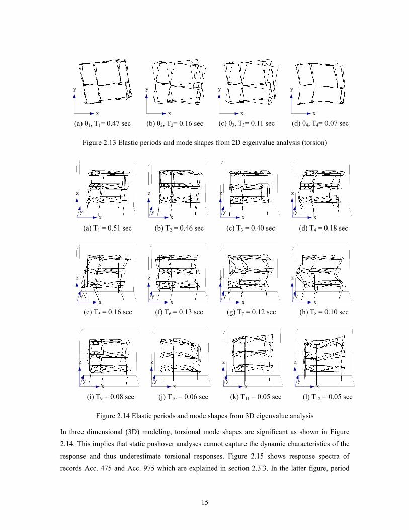
2.3.2 Periods and mode shapes In order to understand the overall response of the structure, periods and mode shapes are obtained through eigenvalue analyses using both 2D and 3D modeling as presented in Table 2.4, Figure 2.11, Figure 2.12, Figure 2.13 and Figure 2.14.

14

Table 2.4 Elastic periods and modeshapes

Models No. Frequencies (rad/sec) Periods (sec) Characteristics Mode shapes 1 13.1 0.48 Horizontal 1 (x1) Figure 2.11 (a) 2 37.0 0.17 Horizontal 2 (x2) Figure 2.11 (b) 3 57.1 0.11 Horizontal 3 (x3) Figure 2.11 (c)

2D, x

4 104.7 0.06 Vertical 1 (z1x) Figure 2.11 (d) 1 14.6 0.43 Horizontal 1 (y1) Figure 2.12 (a) 2 44.9 0.14 Horizontal 2 (y2) Figure 2.12 (b) 3 69.8 0.09 Horizontal 3 (y3) Figure 2.12 (c) 2D, y

4 104.7 0.06 Vertical 1 (z1y) Figure 2.12 (d) 1 13.4 0.47 Rotation 1 (θ1) Figure 2.13 (a) 2 39.3 0.16 Rotation 2 (θ2) Figure 2.13 (b) 3 57.1 0.11 Rotation 3 (θ3) Figure 2.13 (c) 2D, θ

4 89.8 0.07 Rotation 4 (θ4) Figure 2.13 (d) 1 12.3 0.51 Combined (θ1, x1, y1) Figure 2.14 (a) 2 13.7 0.46 Combined (θ1, x1, y1) Figure 2.14 (b) 3 15.7 0.40 Combined (θ1, x1, y1) Figure 2.14 (c) 4 34.9 0.18 Combined (θ2, x1, y1) Figure 2.14 (d) 5 39.3 0.16 Combined (θ2, x1, x2, y1, y2) Figure 2.14 (e) 6 48.3 0.13 Combined (θ2, x2, y2) Figure 2.14 (f) 7 52.4 0.12 Combined (θ3, x2, x3, y2, y3) Figure 2.14 (g) 8 62.8 0.10 Combined (θ3, x2, x3, y2, y3) Figure 2.14 (h) 9 78.5 0.08 Combined (θ3, x3, y3) Figure 2.14 (i)

10 104.7 0.06 Vertical 1 (z1) Figure 2.14 (j) 11 125.7 0.05 Vertical 2 (z2) Figure 2.14 (k)

3D

12 125.7 0.05 Vertical 3 (z3 ) Figure 2.14 (l)

Figure 2.11 Elastic periods and mode shapes from 2D eigenvalue analysis (x direction)

Figure 2.12 Elastic periods and mode shapes from 2D eigenvalue analysis (y direction)

(a) y1, T1 = 0.43 sec (b) y2, T2 = 0.14 sec (c) y3, T3 = 0.09 sec (d) z1y, T4 = 0.06 sec y

z

y

z

y

z

y

z

(a) x1, T1 = 0.48 sec (b) x2, T2 = 0.17 sec (c) x3, T3 = 0.11 sec (d) z1x, T4 = 0.06 sec x

z

x

z

x

z

x

z

15

Figure 2.13 Elastic periods and mode shapes from 2D eigenvalue analysis (torsion)

Figure 2.14 Elastic periods and mode shapes from 3D eigenvalue analysis

In three dimensional (3D) modeling, torsional mode shapes are significant as shown in Figure 2.14. This implies that static pushover analyses cannot capture the dynamic characteristics of the response and thus underestimate torsional responses. Figure 2.15 shows response spectra of records Acc. 475 and Acc. 975 which are explained in section 2.3.3. In the latter figure, period

x

y

x

y

x

y

x

y

(a) θ1, T1= 0.47 sec (b) θ2, T2= 0.16 sec (c) θ3, T3= 0.11 sec (d) θ4, T4= 0.07 sec

x

z

y x

z

yx

z

y x

z

y

(a) T1 = 0.51 sec (b) T2 = 0.46 sec (c) T3 = 0.40 sec (d) T4 = 0.18 sec

x

z

y x

z

yx

z

y x

z

y

(e) T5 = 0.16 sec (f) T6 = 0.13 sec (g) T7 = 0.12 sec (h) T8 = 0.10 sec

x

z

y x

z

yx

z

y x

z

y

(i) T9 = 0.08 sec (j) T10 = 0.06 sec (k) T11 = 0.05 sec (l) T12 = 0.05 sec

16

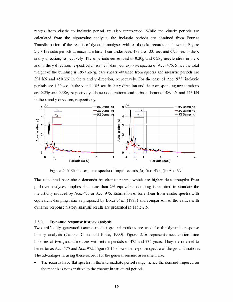
ranges from elastic to inelastic period are also represented. While the elastic periods are calculated from the eigenvalue analysis, the inelastic periods are obtained from Fourier Transformation of the results of dynamic analyses with earthquake records as shown in Figure 2.20. Inelastic periods at maximum base shear under Acc. 475 are 1.00 sec. and 0.95 sec. in the x and y direction, respectively. These periods correspond to 0.20g and 0.23g acceleration in the x and in the y direction, respectively, from 2% damped response spectra of Acc. 475. Since the total weight of the building is 1957 kN/g, base shears obtained from spectra and inelastic periods are 391 kN and 450 kN in the x and y direction, respectively. For the case of Acc. 975, inelastic periods are 1.20 sec. in the x and 1.05 sec. in the y direction and the corresponding accelerations are 0.25g and 0.38g, respectively. These accelerations lead to base shears of 489 kN and 743 kN in the x and y direction, respectively.

Figure 2.15 Elastic response spectra of input records, (a) Acc. 475; (b) Acc. 975

The calculated base shear demands by elastic spectra, which are higher than strengths from pushover analyses, implies that more than 2% equivalent damping is required to simulate the inelasticity induced by Acc. 475 or Acc. 975. Estimation of base shear from elastic spectra with equivalent damping ratio as proposed by Borzi et al. (1998) and comparison of the values with dynamic response history analysis results are presented in Table 2.5.

2.3.3 Dynamic response history analysis Two artificially generated (source model) ground motions are used for the dynamic response history analysis (Campos-Costa and Pinto, 1999). Figure 2.16 represents acceleration time histories of two ground motions with return periods of 475 and 975 years. They are referred to hereafter as Acc. 475 and Acc. 975. Figure 2.15 shows the response spectra of the ground motions. The advantages in using these records for the general seismic assessment are:

• The records have flat spectra in the intermediate period range, hence the demand imposed on the models is not sensitive to the change in structural period.

0

1

2

3

4

5

0 1 2 3 4Periods (sec.)

Acc

eler

atio

n (g

)

0% Damping2% Damping5% DampingTz

Tx

Tθ

(b)

0

1

2

3

4

5


Acc

eler

atio

n (g

)

0% Damping2% Damping5% DampingTz

Tx

Tθ

(a)

17

• They were used in pre-test analysis and actual testing of the full scale ICONS frame (Pinho and Elnashai, 2001; Pinto et al, 2002).

• They represent clearly-defined return period earthquakes that match well two performance targets, damage control (475 year return period) and collapse prevention (975 year return period).

-0.4

-0.2

0

0.2

0.4

0 3 6 9 12 15

Time (sec.)

Acc

eler

atio

n (g

)

-0.4

-0.2

0

0.2

0.4

0 3 6 9 12 15

Time (sec.)A

ccel

erat

ion

(g)

(a) Acc. 475 (b) Acc. 975

Figure 2.16 Acceleration time histories of input records

Smaller displacement in the y direction from Figure 2.17 and Figure 2.18 can be explained by the fact that the building is stiffer and stronger in the y direction than in the x direction, as observed from results of static pushover analyses in Figure 2.8. Figure 2.8 also shows that the difference in stiffness and strength between positive loading and negative loading is negligible in the x direction, while this difference is significant at large displacement in the y direction. Therefore, Figure 2.17 and Figure 2.18 show that variation in response according to loading direction becomes clear when Acc. 975 is applied in the y direction, otherwise responses under positive loading are almost mirror images of negative loading cases.

-100-80-60-40-20

020406080

100

0 3 6 9 12 15

Time (sec.)

Top

disp

lace

men

t (m

m)

-500-400-300-200-100

0100200300400500

0 3 6 9 12 15

Time (sec.)

Bas

e sh

ear (

kN)

(a) Top displacement (Acc. 475, x-positive) (b) Base shear (Acc. 475, x-positive)

Figure 2.17 Top displacement at C3 and base shear time histories - Acc. 475

18

-100-80-60-40-20

020406080

100

0 3 6 9 12 15

Time (sec.)

Top

disp

lace

men

t (m

m)

-500-400-300-200-100

0100200300400500

0 3 6 9 12 15

Time (sec.)

Bas

e sh

ear (

kN)

(c) Top displacement (Acc. 475, x-negative) (d) Base shear (Acc. 475, x-negative)

-100-80-60-40-20

020406080

100

0 3 6 9 12 15

Time (sec.)

Top

disp

lace

men

t (m

m)

-500-400-300-200-100

0100200300400500

0 3 6 9 12 15

Time (sec.)

Bas

e sh

ear (

kN)

(e) Top displacement (Acc. 475, y-positive) (f) Base shear (Acc. 475, y-positive)

-100-80-60-40-20

020406080

100

0 3 6 9 12 15

Time (sec.)

Top

disp

lace

men

t (m

m)

-500-400-300-200-100

0100200300400500

0 3 6 9 12 15

Time (sec.)

Bas

e sh

ear (

kN)

(g) Top displacement (Acc. 475, y-negative) (h) Base shear (Acc. 475, y-negative)

Figure 2.17 Top displacement at C3 and base shear time histories - Acc. 475 (continued)

19

-100-80-60-40-20

020406080

100

0 3 6 9 12 15

Time (sec.)

Top

disp

lace

men

t (m

m)

-500-400-300-200-100

0100200300400500

0 3 6 9 12 15

Time (sec.)

Bas

e sh

ear (

kN)

(a) Top displacement (Acc. 975, x-positive) (b) Base shear (Acc. 975, x-positive)

-100-80-60-40-20

020406080

100

0 3 6 9 12 15

Time (sec.)

Top

disp

lace

men

t (m

m)

-500-400-300-200-100

0100200300400500

0 3 6 9 12 15

Time (sec.)

Bas

e sh

ear (

kN)

(c) Top displacement (Acc. 975, x-negative) (d) Base shear (Acc. 975, x-negative)

-100-80-60-40-20

020406080

100

0 3 6 9 12 15

Time (sec.)

Top

disp

lace

men

t (m

m)

-500-400-300-200-100

0100200300400500

0 3 6 9 12 15

Time (sec.)

Bas

e sh

ear (

kN)

(e) Top displacement (Acc. 975, y-positive) (f) Base shear (Acc. 975, y-positive)

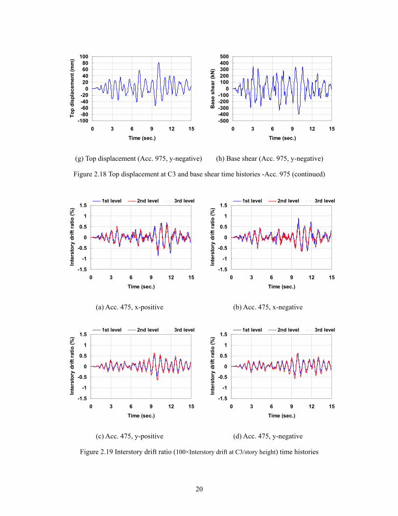
Figure 2.18 Top displacement at C3 and base shear time histories - Acc. 975

20

-100-80-60-40-20

020406080

100

0 3 6 9 12 15

Time (sec.)

Top

disp

lace

men

t (m

m)

-500-400-300-200-100

0100200300400500

0 3 6 9 12 15

Time (sec.)

Bas

e sh

ear (

kN)

(g) Top displacement (Acc. 975, y-negative) (h) Base shear (Acc. 975, y-negative)

Figure 2.18 Top displacement at C3 and base shear time histories -Acc. 975 (continued)

-1.5

-1

-0.5

0

0.5

1

1.5

0 3 6 9 12 15

Time (sec.)

Inte

rsto

ry d

rift r

atio

(%)

1st level 2nd level 3rd level

-1.5

-1

-0.5

0

0.5

1

1.5

0 3 6 9 12 15

Time (sec.)

Inte

rsto

ry d

rift r

atio

(%)


(a) Acc. 475, x-positive (b) Acc. 475, x-negative

-1.5

-1

-0.5

0

0.5

1

1.5

0 3 6 9 12 15

Time (sec.)

Inte

rsto

ry d

rift r

atio

(%)


-1.5

-1

-0.5

0

0.5

1

1.5

0 3 6 9 12 15

Time (sec.)

Inte

rsto

ry d

rift r

atio

(%)


(c) Acc. 475, y-positive (d) Acc. 475, y-negative

Figure 2.19 Interstory drift ratio (100×Interstory drift at C3/story height) time histories

21

-1.5

-1

-0.5

0

0.5

1

1.5

0 3 6 9 12 15

Time (sec.)

Inte

rsto

ry d

rift r

atio

(%)


-1.5

-1

-0.5

0

0.5

1

1.5

0 3 6 9 12 15

Time (sec.)

Inte

rsto

ry d

rift r

atio

(%)


(e) Acc. 975, x-positive (f) Acc. 975, x-negative

-1.5

-1

-0.5

0

0.5

1

1.5

0 3 6 9 12 15

Time (sec.)

Inte

rsto

ry d

rift r

atio

(%)


-1.5

-1

-0.5

0

0.5

1

1.5

0 3 6 9 12 15

Time (sec.)

Inte

rsto

ry d

rift r

atio

(%)


(g) Acc. 975, y-positive (h) Acc. 975, y-negative

Figure 2.19 Interstory drift ratio (100×Interstory drift at C3/story height) time histories (continued)

All response time histories (Figure 2.17, Figure 2.18 and Figure 2.19) show a smaller magnitude and shorter period between 6 and 9 seconds. This is due to the characteristics of ground motions. At that point, the period of ground motion is close to the higher mode period of the structure and hence participation of higher modes becomes larger. Inelastic periods of the structure are obtained by Fourier transformation and period time histories of the structure are plotted in Figure 2.20. Since the period of a structure becomes longer as inelastic response of the structure increases, this can be a measure of structural degradation. Comparing Figure 2.20 (a) and results from dynamic response history analyses (Figure 2.17, Figure 2.18 and Figure 2.19) reveals that as top displacement and interstory drift response of the structure increase, the periods become longer. And the x directional response under Acc. 975 shows the longest period because it has the largest displacement which causes the largest inelasticity.

22

0

0.2

0.4

0.6

0.8

1

1.2

1.4

0 3 6 9 12 15Time (sec.)

Perio

d (s

ec.)

Acc. 475 xAcc. 475 yAcc. 975 xAcc. 975 y

0

0.1

0.2

0.3


Four

ier a

mpl

itude

Acc. 475Acc. 975

Tz

Tx

(a) Period time histories of the structure (b) Fourier amplitude spectra for the input records

Figure 2.20 Inelastic periods of the structure

Inelastic response of structures can be conveniently related to elastic response spectra with damping using the relationships between ductility and equivalent damping ratios proposed by Borzi et al. (1998, 2001) as shown in Figure 2.21.

0

5

10

15

20

1 2 3 4 5 6Ductility

Equi

vale

nt d

ampi

ng ra

tio (%

)

EPPHSS, K3=0HSS, K3=10% KyHSS, K3=-20% KyHSS, K3=-30% Ky

Figure 2.21 Relationship between ductility and equivalent damping ratios

Borzi's method is utilized as an approximate method to check the base shear obtained from dynamic analyses. This method is based on the relationship between ductility and equivalent damping for an assumed primary curve which is same as pushover curve. The primary curve in the x direction is assumed to be hysteretic hardening-softening (HSS) model with K3=-20% Ky, which means softening after the peak strength. K3 and Ky are post-yield and before-yield stiffness, respectively. In the y direction, the primary curve is assumed to be HSS with K3=0. Displacements corresponding to maximum base shears are obtained from capacity curves in Figure 2.8 and dividing them by yield displacements gives the ductility factors. Yield displacement is calculated by the method described in Section 3.2.1. Equivalent damping ratios are obtained from Figure 2.21 according to the above calculated ductility factors. Then, with the

23

equivalent damping and the corresponding response spectra, base shears can be calculated by multiplying the total mass (1957 kN/g) of the building to the spectral accelerations in Figure 2.22. Details of the calculation procedures are presented in Table 2.5. The difference between base shears (M × Sa in Table 2.5) calculated by response spectra with equivalent damping ratios and the values (Vmax in Table 2.5) obtained from dynamic response history analyses are less than 7%.

0

0.2

0.4

0.6

0.8


Acc

eler

atio

n (g

)

4.0% Damping5.4% Damping

475x475y

0

0.2

0.4

0.6

0.8


Acc

eler

atio

n (g

)

8.0% Damping10.2% Damping

475x475y

(a) Acc. 475 (b) Acc. 975

Figure 2.22 Acceleration response spectra with equivalent damping ratios

Table 2.5 Base shear calculation from elastic response spectra

Acc. 475x 475y 975x 975y

Vmax (kN) 333 [Figure 2.17(b)] 370 [Figure 2.17(f)] 352 [Figure 2.18(b)] 435 [Figure 2.18(f)]

T at Vmax (sec) 1.00 [Figure 2.20(a)] 0.95 [Figure 2.20(a)] 1.20 [Figure 2.20(a)] 1.05 [Figure 2.20(a)]

∆ at Vmax (mm) 60 [Figure 2.8] 65.8 [Figure 2.8] 75 [Figure 2.8] 84 [Figure 2.8]

∆y (mm) 45 50 45 50

Ductility 1.33 1.32 1.67 1.68

Equivalent

damping (%) 5.4 [Figure 2.21] 4.0 [Figure 2.21] 10.2 [Figure 2.21] 8.0 [Figure 2.21]

Sa (g) 0.175 [Figure 2.22 (a)] 0.202 [Figure 2.22 (a)] 0.188 [Figure 2.22 (b)] 0.226 [Figure 2.22 (b)]

M × Sa (kN) 342.5 395.3 367.9 442.3

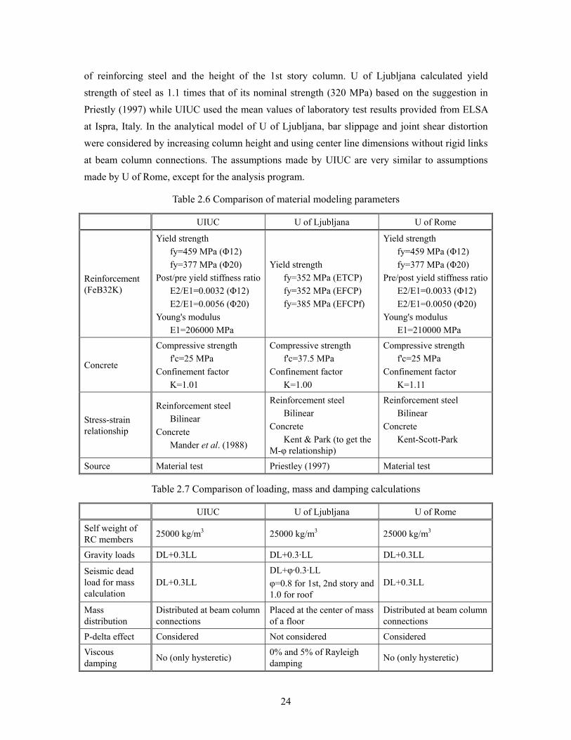
2.3.4 Comparison of modeling assumptions and results The pre-test analyses were carried out by three institutions; University of Illinois at Urbana-Champaign (UIUC), University of Ljubljana (U of Ljubljana; Stratan and Fajfar, 2002) and University of Rome "La Sapienza" (U of Rome; Franchin et al., 2003). The modeling assumptions by three institutions are compared in Table 2.6, Table 2.7 and Table 2.8. Between U of Ljubljana and UIUC, major discrepancies exist in the assumption of yield strength

24

of reinforcing steel and the height of the 1st story column. U of Ljubljana calculated yield strength of steel as 1.1 times that of its nominal strength (320 MPa) based on the suggestion in Priestly (1997) while UIUC used the mean values of laboratory test results provided from ELSA at Ispra, Italy. In the analytical model of U of Ljubljana, bar slippage and joint shear distortion were considered by increasing column height and using center line dimensions without rigid links at beam column connections. The assumptions made by UIUC are very similar to assumptions made by U of Rome, except for the analysis program.

Table 2.6 Comparison of material modeling parameters

UIUC U of Ljubljana U of Rome

Reinforcement (FeB32K)

Yield strength fy=459 MPa (Φ12) fy=377 MPa (Φ20) Post/pre yield stiffness ratio E2/E1=0.0032 (Φ12) E2/E1=0.0056 (Φ20) Young's modulus E1=206000 MPa

Yield strength fy=352 MPa (ETCP) fy=352 MPa (EFCP) fy=385 MPa (EFCPf)

Yield strength fy=459 MPa (Φ12) fy=377 MPa (Φ20) Pre/post yield stiffness ratio E2/E1=0.0033 (Φ12) E2/E1=0.0050 (Φ20) Young's modulus E1=210000 MPa

Concrete

Compressive strength f'c=25 MPa Confinement factor K=1.01

Compressive strength f'c=37.5 MPa Confinement factor K=1.00

Compressive strength f'c=25 MPa Confinement factor K=1.11

Stress-strain relationship

Reinforcement steel Bilinear Concrete Mander et al. (1988)

Reinforcement steel Bilinear Concrete Kent & Park (to get the M-φ relationship)

Reinforcement steel Bilinear Concrete Kent-Scott-Park

Source Material test Priestley (1997) Material test

Table 2.7 Comparison of loading, mass and damping calculations


Self weight of RC members 25000 kg/m3 25000 kg/m3 25000 kg/m3

Gravity loads DL+0.3LL DL+0.3·LL DL+0.3LL

Seismic dead load for mass calculation

DL+0.3LL DL+φ·0.3·LL φ=0.8 for 1st, 2nd story and 1.0 for roof

DL+0.3LL

Mass distribution

Distributed at beam column connections

Placed at the center of mass of a floor

Distributed at beam column connections

P-delta effect Considered Not considered Considered

Viscous damping No (only hysteretic) 0% and 5% of Rayleigh

damping No (only hysteretic)

25

Table 2.8 Comparison of assumptions in element modeling


Analysis program ZeusNL CANNY OpenSees

Element model Distributed plasticity model

One-component lumped plasticity model with tri-linear moment-rotation envelope (ETCP)

Distributed plasticity model with flexibility formulation (5 Lobatto integration points)

Centerline dimensions Yes Yes Yes

Rigid offset at beam column connection

Yes No Yes

Additional deformations at element intersections and footing interface

Not considered

Bar slippage and joint shear distortion were considered by increasing column height and using center line dimensions without rigid members at beam column connections.

Not considered

M-M-N interaction Yes ETCP (no), EFCP ( yes) Yes (3D fiber section)

Effective width Beam width plus 7% of the clear span of the beam on either side of the web

Paulay and Priestley (1992) Beam width plus 7% of the clear span of the beam on either side of the web

Height of 1st story column 2.75 m 2.75 m +0.25 m (for bar

slippage at footing) 2.75 m

In order to investigate the differences among analysis results from three institutions, four different strengths of the structure according to the directions of loading presented in Figure 2.23 are compared in Table 2.9 and Figure 2.24.

Figure 2.23 Directions of loading

x (+)

y (+)

x (-)

y (-)

V4

V3 V2

V1

x

y

26

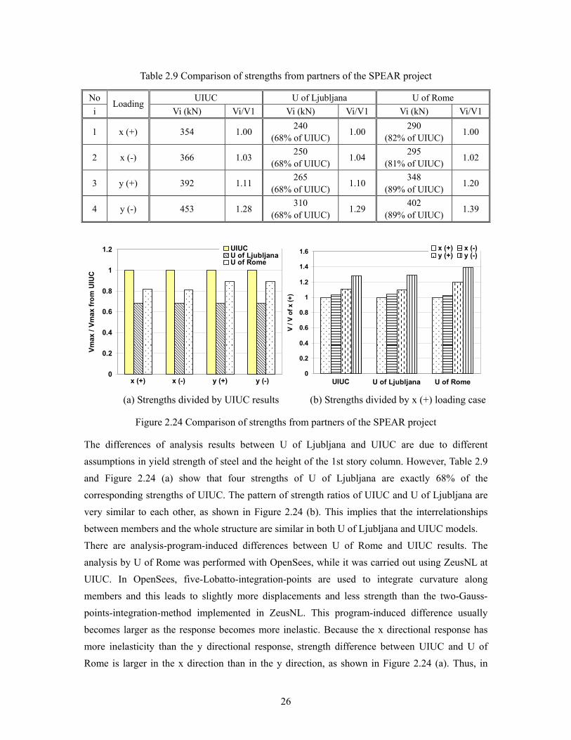
Table 2.9 Comparison of strengths from partners of the SPEAR project

No UIUC U of Ljubljana U of Rome i

Loading Vi (kN) Vi/V1 Vi (kN) Vi/V1 Vi (kN) Vi/V1

1 x (+) 354 1.00 240 (68% of UIUC) 1.00 290

(82% of UIUC) 1.00

2 x (-) 366 1.03 250 (68% of UIUC) 1.04 295

(81% of UIUC) 1.02

3 y (+) 392 1.11 265 (68% of UIUC) 1.10 348

(89% of UIUC) 1.20

4 y (-) 453 1.28 310 (68% of UIUC) 1.29 402

(89% of UIUC) 1.39

0

0.2

0.4

0.6

0.8

1

1.2

Vmax

/ Vm

ax fr

om U

IUC

UIUCU of LjubljanaU of Rome

x (+) x (-) y (+) y (-)0

0.2

0.4

0.6

0.8

1

1.2

1.4

1.6

V / V

of x

(+)

x (+) x (-)y (+) y (-)

UIUC U of RomeU of Ljubljana (a) Strengths divided by UIUC results (b) Strengths divided by x (+) loading case

Figure 2.24 Comparison of strengths from partners of the SPEAR project

The differences of analysis results between U of Ljubljana and UIUC are due to different assumptions in yield strength of steel and the height of the 1st story column. However, Table 2.9 and Figure 2.24 (a) show that four strengths of U of Ljubljana are exactly 68% of the corresponding strengths of UIUC. The pattern of strength ratios of UIUC and U of Ljubljana are very similar to each other, as shown in Figure 2.24 (b). This implies that the interrelationships between members and the whole structure are similar in both U of Ljubljana and UIUC models. There are analysis-program-induced differences between U of Rome and UIUC results. The analysis by U of Rome was performed with OpenSees, while it was carried out using ZeusNL at UIUC. In OpenSees, five-Lobatto-integration-points are used to integrate curvature along members and this leads to slightly more displacements and less strength than the two-Gauss-points-integration-method implemented in ZeusNL. This program-induced difference usually becomes larger as the response becomes more inelastic. Because the x directional response has more inelasticity than the y directional response, strength difference between UIUC and U of Rome is larger in the x direction than in the y direction, as shown in Figure 2.24 (a). Thus, in

27

Figure 2.24 (b), U of Rome shows larger y directional strength ratio than U of Ljubljana or UIUC. Maximum interstory drift ratios are compared in Figure 2.25 and Table 2.10. The interstory drifts are obtained from dynamic response history analyses performed with the Montenegro 1979 - Herceg Novi record, in the loading direction-D1 and four different intensities (0.05g, 0.2g, 0.3g and 0.35g). Details on the input record are represented in Section 4.1. U of Ljubljana showed relatively smaller interstory drift than UIUC while U of Rome provided larger interstory drifts than UIUC. The maximum difference is 48% in the case of 0.05g-y direction.

Table 2.10 Comparison of maximum interstory drift ratios (IDR)

Montenegro 1979 - Herceg Novi, D1 (Figure 4.7)

PGA 0.20 0.30 0.05 0.35

Direction of ID x y x y x y x y

UIUC (%) 1.37 1.05 1.86 1.87 0.27 0.23 2.36 2.10

U of Ljubljana (%) 0.98 0.84 1.64 0.98 - - - -

U of Rome (%) - - - - 0.36 0.34 3.30 1.80

Max. 1st story IDR

Other institutions/UIUC 0.72 0.80 0.88 0.53 1.33 1.48 1.40 0.86

UIUC (%) 1.24 1.25 1.65 1.60 0.33 0.27 1.50 1.80

U of Ljubljana (%) 1.18 0.91 1.85 1.56 - - - -

U of Rome (%) - - - - 0.37 0.42 1.30 2.00 Max. 2nd story

IDR


UIUC (%) 0.72 0.78 0.96 1.10 0.28 0.22 1.10 1.16

U of Ljubljana (%) 0.69 0.91 0.69 1.24 - - - -

U of Rome (%) - - - - 0.3 0.27 1.5 1.3 Max. 3rd story

IDR


(a) U of Ljubljana divided by UIUC (b) U of Rome divided by UIUC

Figure 2.25 Comparison of maximum interstory drift ratios (IDR) from dynamic response history analyses performed by three institutions (UIUC, U of Ljubljana and U of Rome)

0

0.2

0.4

0.6

0.8

1

1.2

1.4

1.6

U o

f Lju

blja

na /

UIU

C

1st story ID2nd story ID3rd story ID

0.20g, x 0.20g, z 0.30g, x 0.30g, z0.20g, x 0.20g, y 0.30g, x 0.30g, y0

0.2

0.4

0.6

0.8

1

1.2

1.4

1.6

U o

f Rom

e / U

IUC

1st story ID2nd story ID3rd story ID

0.05g, x 0.05g, z 0.35g, x 0.35g, z0.05g, x 0.05g, y 0.35g, x 0.35g, y

28

3. DAMAGE ASSESSMENT

The state of damage resulting from earthquakes can be described by damage indices. Since damage of RC structures are generally related to inelastic deformation, deformation-based damage indices are more appropriate for this report than force-based ones. Although measuring response is relatively easy, deciding on a single value as a specific damage state of a building is difficult. Thus, deformation parameters for damage criteria and limit states are defined before the damage assessment of the test building is performed.

3.1. MEMBER LEVEL DAMAGE CRITERIA

3.1.1 Curvature ductility Ductility is a measure of the ability to deform beyond the elastic limit without significant degradation of strength. Curvature ductility is defined as Equation 3.1.

ym / φφ=µφ (3.1)

where φm is the imposed section curvature and φy is the yield curvature. Yield curvature and ultimate curvature are defined by Equation 3.2 and Equation 3.3, respectively.

)Xd/( yyy −ε=φ (3.2)

where, εy is the yield strain of longitudinal reinforcement, d is the distance between top fiber of concrete and the reinforcing bar, Xy is the neural axis depth at the corresponding state.

u

cuu X

ε=φ (3.3)

where, εcu is the ultimate compression strain of the confined concrete and Xu is the neural axis depth at the ultimate state. The neutral axis depth Xu is the distance between the neutral axis and the extreme fiber of the confined region. The cover concrete is unconfined and will eventually become ineffective after the compressive strength is attained, but the core concrete will continue to carry stress at high strains (Mander et al, 1988). Thus, the unconfined concrete around the confined core should be neglected in the calculation of ultimate curvature.

3.1.2 Curvature Limit States Curvature of a section is the most accurate measure of flexural behavior of a member while rotation varies according to the moment distribution along a unit length, and displacements are influenced by the moment distribution along the member length. Since yield and ultimate curvatures are based on the axial strain of fibers in the section of a member, axial forces have a

29

significant influence on the flexural capacity of members. For simplicity of calculation, axial forces in beams are ignored and axial forces on columns are calculated based on the gravity loads, ignoring the variation of axial forces due to the overturning moment by the lateral loads. In order to calculate the yield and ultimate curvature under various axial force conditions, a nonlinear analysis program, ZeusNL, is utilized. Calculated yield curvatures and ultimate curvatures are represented in Table 3.1 and Table 3.2. As shown in Figure 2.3 (b), the amount of longitudinal reinforcement in a beam varies along its length. Considering the bent up of reinforcing bar at ends of beams and the difference in quantity of steel bar between top and bottom reinforcement, curvature limit states are calculated separately for center and both ends of a beam in Table 3.2; end_1 is the left or down side end, and end_2 is the right or up side end in Figure 2.1 (b).

Table 3.1 Yield and ultimate curvatures of columns (εcu=0.003)

Member Story Axial force (kN)

Yield curvature (φy, rad/mm×106)

Ultimate curvature (φu, rad/mm×106)

Ductility limit (φu/φy)

1 234.22 17.50 38.78 2.22 2 154.46 16.16 54.56 3.38 C1 3 74.98 15.53 94.24 6.07 1 252.67 18.73 37.29 1.99 2 166.54 16.20 51.33 3.17 C2 3 80.13 15.59 89.77 5.76 1 407.26 21.53 28.29 1.31 2 272.34 18.76 35.07 1.87 C3 3 139.62 16.09 60.08 3.73 1 328.72 17.79 31.55 1.77 2 217.96 17.49 40.73 2.33 C4 3 107.89 15.87 73.29 4.62 1 89.56 15.68 84.26 5.37 2 57.42 15.34 112.11 7.31 C5 3 25.43 15.26 165.93 10.87 1 216.44 14.74 17.25 345.07 95.21 23.41 5.52 2 141.29 13.79 16.61 237.00 115.12 17.19 6.93 C6 3 64.29 13.43 16.02 439.45 144.02 32.71 8.99 1 150.45 16.14 55.61 3.44 2 98.51 15.77 78.81 5.00 C7 3 45.90 15.31 125.64 8.20 1 73.66 15.51 95.35 6.15 2 45.72 15.31 125.63 8.20 C8 3 18.66 14.16 179.40 12.67 1 182.26 17.40 48.26 2.77 2 121.37 15.98 66.56 4.17 C9 3 59.05 15.35 109.82 7.16

30

Table 3.2 Yield and ultimate curvatures of beams (εcu=0.003)



Ductility limit (φu/φy) Member Section

positive negative positive negative positive negative center 6.20 6.35 62.42 62.05 10.07 9.76 end_1 5.78 6.87 51.47 51.47 8.91 7.49 B1 end_2 5.73 7.51 42.79 42.79 7.47 5.70 center 6.02 6.31 50.48 50.48 8.39 8.01 end_1 5.57 7.08 36.33 36.33 6.52 5.13 B2 end_2 5.52 7.71 31.78 31.78 5.76 4.12 center 5.73 6.33 37.41 37.41 6.53 5.91 end_1 5.58 7.07 32.91 32.91 5.90 4.65 B3 end_2 5.58 7.07 32.91 32.91 5.90 4.65 center 6.44 5.93 33.26 33.26 5.17 5.61 end_1 5.86 9.06 16.14 16.14 2.75 1.78 end_2 5.86 9.06 16.14 16.14 2.75 1.78

B4

end_* 5.88 8.74 17.66 17.66 3.00 2.02 center 6.20 6.35 62.05 62.05 10.01 9.76 end_1 5.78 6.87 51.47 51.47 8.91 7.49 B5 end_2 5.78 6.87 51.47 51.47 8.91 7.49 center 5.77 6.29 48.23 48.23 8.36 7.67 end_1 5.59 7.08 32.91 33.29 5.89 4.70 B6 end_2 5.62 7.03 35.56 35.56 6.33 5.06 center 6.14 5.92 42.22 42.22 6.87 7.13 end_1 5.82 8.74 17.66 17.66 3.04 2.02 B7 end_2 5.83 8.45 18.05 18.05 3.10 2.14 center 5.55 6.26 48.95 48.58 8.82 7.75 end_1 5.39 7.02 31.38 31.38 5.82 4.47 B8 end_2 5.39 7.02 31.38 31.38 5.82 4.47 center 6.15 6.23 27.26 27.26 4.43 4.38 end_1 5.79 9.36 16.14 16.14 2.79 1.72 end_2 5.59 7.84 19.95 19.95 3.57 2.55

B9

end_* 5.78 9.37 16.14 16.14 2.79 1.72 center 5.79 6.53 34.02 34.02 5.88 5.21 end_1 5.37 7.03 29.48 29.48 5.49 4.20 B10 end_2 5.57 7.90 24.54 24.54 4.41 3.11 center 5.75 6.30 48.24 48.24 8.38 7.66 end_1 5.60 6.79 36.32 36.32 6.48 5.35 B11 end_2 5.53 7.70 30.25 30.25 5.47 3.93 center 5.74 6.31 50.48 50.48 8.79 8.01 end_1 5.59 6.81 37.84 37.84 6.77 5.56 B12 end_2 5.53 7.42 33.29 33.29 6.02 4.49

* end_1: left or down side end; end_2: right or up side end; end_*: short part between the connection of the

intersecting beam and the beam-column connection, refer to Figure 2.1 (b)

The large variation in beam ductility is due to the variation in effective widths (Table 2.1) and reinforcing steel ratios. When calculating curvatures in Table 3.1 and Table 3.2, ultimate strain of

31

concrete was assumed to be 0.003. Additional information on curvature limit states with higher

ultimate strains of concrete (0.0035 and 0.00456) is presented in Appendix A.

3.1.3 Member shear capacity A shear strength model suggested by Priestley et al. (1994) is utilized to obtain the shear supply of members. Shear strength consists of three components,

psc VVVV ++= (3.4)

where Vc is the concrete component, Vs is the truss mechanism component by stirrups and Vp is the axial load component. Vc and Vs are given by:

)A8.0(fkV grosscc = °= 30cots

'DfAV yv

s (3.5)

where k is determined by curvature of the member and Av is the total transverse reinforcement area per stirrup spacing s, and D' is the distance between centers of the peripheral hoops in the direction parallel to the applied shear force. In this report, Vp is ignored because the axial load component is very small for slender columns.

3.2. STRUCTURE LEVEL DAMAGE CRITERIA

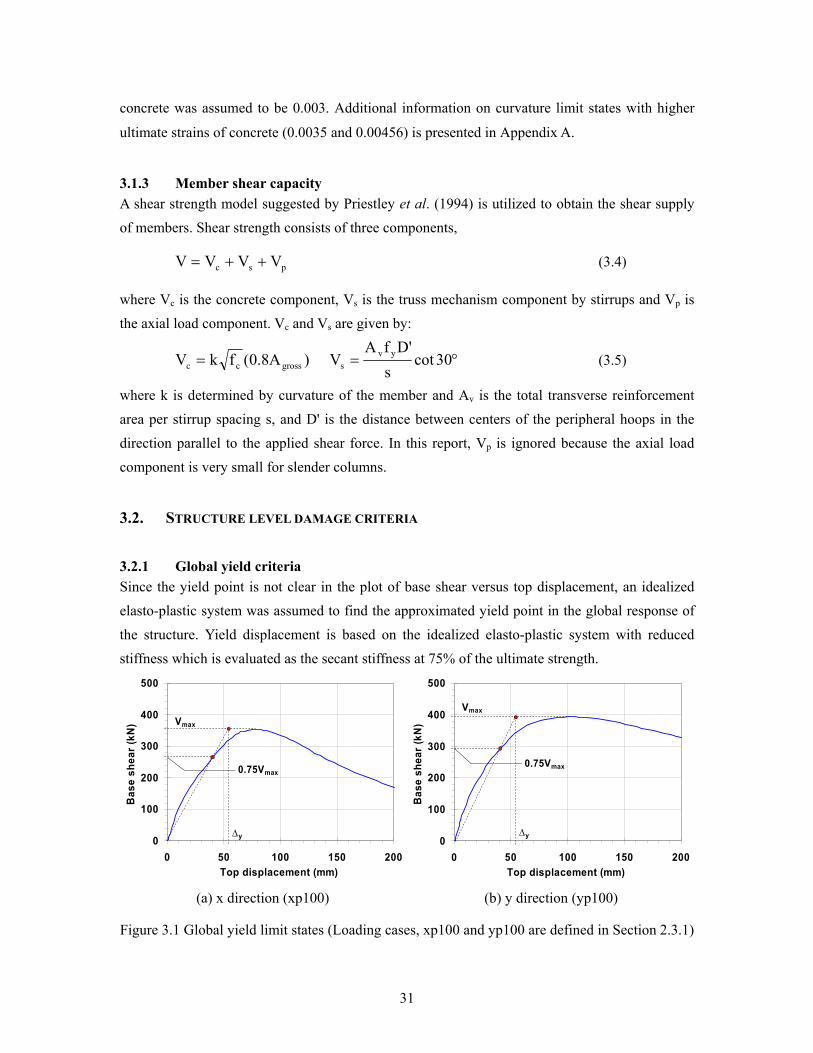
3.2.1 Global yield criteria Since the yield point is not clear in the plot of base shear versus top displacement, an idealized elasto-plastic system was assumed to find the approximated yield point in the global response of the structure. Yield displacement is based on the idealized elasto-plastic system with reduced stiffness which is evaluated as the secant stiffness at 75% of the ultimate strength.

0

100

200

300

400

500

0 50 100 150 200Top displacement (mm)

Bas

e sh

ear (

kN) Vmax

0.75Vmax

∆y 0

100

200

300

400

500


Bas

e sh

ear (

kN)

Vmax

∆y

0.75Vmax

(a) x direction (xp100) (b) y direction (yp100)

Figure 3.1 Global yield limit states (Loading cases, xp100 and yp100 are defined in Section 2.3.1)

32

From Figure 3.1, the yield displacement (∆y) of the test model is 54 mm in the x direction and 53 mm in the y direction. They are 0.60% and 0.59% of the height of the structure, respectively. Global yield points on the capacity curves with negative directional loadings ('xn100' and 'yn100') are presented in Appendix B.

3.2.2 Global failure criteria 3.2.2.1. Interstory drift On the structure level, the interstory drift (ID) is one of the simplest and most commonly used damage indicators. This is defined as:

i

1iii h

ID −∆−∆= (3.6)

where Δi − Δi-1 is the relative displacement between successive stories and hi is the story height. Several ID values corresponding to collapse for a building have been suggested by different researchers. At values in excess of the collapse limit, it is assumed that significant p-∆ effect leads to failure of a building. An ID of 2% has been suggested by Sozen (1981) as the collapse limit for three-quarters of RC buildings and 2.5% was suggested by SEAOC (1995) as shown in Table 3.3. In studies by Broderick and Elnashai (1994) and Kappos (1997), 3% was recommended as an upper limit of ID. However, the structure under consideration in this report is not built with modern seismic codes and it will be weaker than those structures used in previous studies to obtain 3% ID limit. Figure 3.2 shows a statistical distribution for the critical ID by Dymiotis (2000). This data is based on the experimental results obtained from the literature. From Figure 3.2, 2.5 % ID is the lower tail of the statistical distribution of interstory drift at failure. This is a more conservative value than the 3 % ID limit for buildings designed by seismic code and same as the ID limit at collapse suggested by SEAOC. Therefore, 2.5 % is assumed as an appropriate ID limit at collapse for the structure in this report.

Figure 3.2 Statistical distribution of critical drift (Dymiotis, 2000)

33

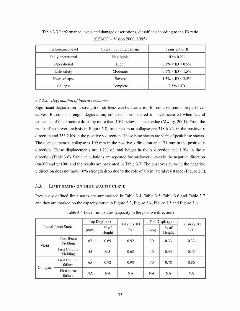
Table 3.3 Performance levels and damage descriptions, classified according to the ID ratio (SEAOC – Vision 2000, 1995)

Performance level Overall building damage Transient drift

Fully operational Negligible ID < 0.2%

Operational Light 0.2% < ID < 0.5%

Life safety Moderate 0.5% < ID < 1.5%

Near collapse Severe 1.5% < ID < 2.5%

Collapse Complete 2.5% < ID

3.2.2.2. Degradation of lateral resistance Significant degradation in strength or stiffness can be a criterion for collapse points on pushover curves. Based on strength degradation, collapse is considered to have occurred when lateral resistance of the structure drops by more than 10% below its peak value (Mwafy, 2001). From the result of pushover analysis in Figure 2.8, base shears at collapse are 318.6 kN in the positive x direction and 353.2 kN in the positive y direction. These base shears are 90% of peak base shears. The displacement at collapse is 109 mm in the positive x direction and 171 mm in the positive y direction. These displacements are 1.2% of total height in the x direction and 1.9% in the y direction (Table 3.6). Same calculations are repeated for pushover curves in the negative direction (xn100 and yn100) and the results are presented in Table 3.7. The pushover curve in the negative y direction does not have 10% strength drop due to the role of C6 in lateral resistance (Figure 2.8).

3.3. LIMIT STATES ON THE CAPACITY CURVE

Previously defined limit states are summarized in Table 3.4, Table 3.5, Table 3.6 and Table 3.7 and they are marked on the capacity curve in Figure 3.3, Figure 3.4, Figure 3.5 and Figure 3.6.

Table 3.4 Local limit states (capacity in the positive direction)

Top Displ. (x) Top Displ. (y) Local Limit States

(mm) % of Height

1st story ID (%) (mm) % of

Height

1st story ID (%)

First Beam Yielding 62 0.69 0.92 30 0.33 0.33

Yield First Column

Yielding 45 0.5 0.62 40 0.44 0.45

First Column failure 65 0.72 0.98 70 0.78 0.86

Collapse First shear

failure NA NA NA NA NA NA

34

Table 3.5 Local limit states (capacity in the negative direction)

Top Displ. (x) Top Displ. (y) Local Limit States

(mm) % of Height

1st story ID (%) (mm) % of

Height

1st story ID (%)

First Beam Yielding 55 0.61 0.76 55 0.61 0.53

Yield First Column

Yielding 41 0.46 0.55 31 0.34 0.27

First Column failure 68 0.64 1.02 74 0.82 0.76

Collapse First shear

failure NA NA NA NA NA NA

Table 3.6 Global limit states (capacity in the positive direction)

Top Displacement (x) Top Displacement (y) Global Limit States (mm) % of Height (mm) % of Height

Yield Displacement at 75% of Peak Strength 54 0.60 53 0.59

2.5% Interstory Drift 106 1.18 157 1.74 Collapse

10% Degradation in Lateral Resistance 109 1.21 171 1.90

Table 3.7 Global limit states (capacity in the negative direction)

Top Displacement (x) Top Displacement (y) Global Limit States (mm) % of Height (mm) % of Height

Yield Displacement at 75% of Peak Strength 55 0.61 58 0.64

2.5% Interstory Drift 109 1.21 152 1.69 Collapse

10% Degradation in Lateral Resistance 121 1.34 NA NA

Since pushover curves cannot reflect the effect of soft story and torsion on member level damage, exact damage assessment of an irregular building under a specific earthquake loading can be achieved by dynamic response history analysis. However, the limit states presented in Table 3.4, Table 3.5, Table 3.6 and Table 3.7 can be useful guidelines to a quick and brief assessment of the capacity of the structure. Figure 3.3, Figure 3.4, Figure 3.5 and Figure 3.6 show that column crushing is followed by global failure limit states in the x and y directions. If the collapse of a building is conservatively defined as a damage stage with a crushed critical column, the failure criteria of this structure is governed by local limit states.

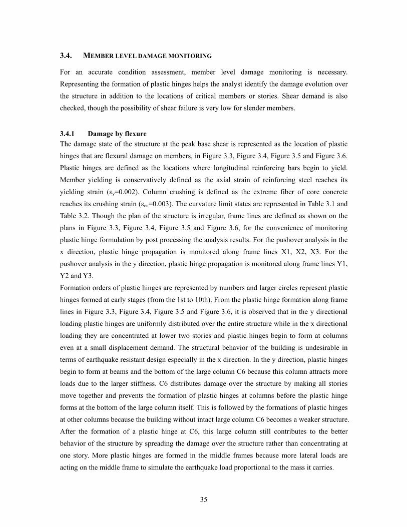
35

3.4. MEMBER LEVEL DAMAGE MONITORING

For an accurate condition assessment, member level damage monitoring is necessary. Representing the formation of plastic hinges helps the analyst identify the damage evolution over the structure in addition to the locations of critical members or stories. Shear demand is also checked, though the possibility of shear failure is very low for slender members.

3.4.1 Damage by flexure The damage state of the structure at the peak base shear is represented as the location of plastic hinges that are flexural damage on members, in Figure 3.3, Figure 3.4, Figure 3.5 and Figure 3.6. Plastic hinges are defined as the locations where longitudinal reinforcing bars begin to yield. Member yielding is conservatively defined as the axial strain of reinforcing steel reaches its yielding strain (εy=0.002). Column crushing is defined as the extreme fiber of core concrete reaches its crushing strain (εcu=0.003). The curvature limit states are represented in Table 3.1 and Table 3.2. Though the plan of the structure is irregular, frame lines are defined as shown on the plans in Figure 3.3, Figure 3.4, Figure 3.5 and Figure 3.6, for the convenience of monitoring plastic hinge formulation by post processing the analysis results. For the pushover analysis in the x direction, plastic hinge propagation is monitored along frame lines X1, X2, X3. For the pushover analysis in the y direction, plastic hinge propagation is monitored along frame lines Y1, Y2 and Y3. Formation orders of plastic hinges are represented by numbers and larger circles represent plastic hinges formed at early stages (from the 1st to 10th). From the plastic hinge formation along frame lines in Figure 3.3, Figure 3.4, Figure 3.5 and Figure 3.6, it is observed that in the y directional loading plastic hinges are uniformly distributed over the entire structure while in the x directional loading they are concentrated at lower two stories and plastic hinges begin to form at columns even at a small displacement demand. The structural behavior of the building is undesirable in terms of earthquake resistant design especially in the x direction. In the y direction, plastic hinges begin to form at beams and the bottom of the large column C6 because this column attracts more loads due to the larger stiffness. C6 distributes damage over the structure by making all stories move together and prevents the formation of plastic hinges at columns before the plastic hinge forms at the bottom of the large column itself. This is followed by the formations of plastic hinges at other columns because the building without intact large column C6 becomes a weaker structure. After the formation of a plastic hinge at C6, this large column still contributes to the better behavior of the structure by spreading the damage over the structure rather than concentrating at one story. More plastic hinges are formed in the middle frames because more lateral loads are acting on the middle frame to simulate the earthquake load proportional to the mass it carries.

36

Figure 3.3 Limit states and plastic hinge formation at peak base shear (positive x direction)

Frame X2

8

9

28

12

3

5

1

15

7

17 13

Frame X1

24

19

27

22

25

20

2

29

10

0

100

200

300

400

500

0 50 100 150 200Top Displacement (mm)

Bas

e sh

ear (

kN)

1st beam yielding 1st column yielding1st column curshing Global yield2.5% ID ratio 10% strength drop

x

y

0.26Vx

0.50Vx

0.24Vx

X3

X2

X1

Frame X3

16

18

26

11

23

4

14

6

21

x

z

37

Figure 3.4 Limit states and plastic hinge formation at peak base shear (negative x direction)

1

2

13

3

29

12

5

4

22

20

32

16

25

18

Frame X3

7

10

26

6

33

30

15

19

14

28

Frame X2 Frame X1

17

31

24

9

11 27

21

23

8

1st beam yielding 1st column yielding1st column curshing Global yield2.5% ID ratio 10% strength drop

0

100

200

300

400

500


Bas

e sh

ear (

kN)

x

z

x

y

0.26Vx

0.50Vx

0.24Vx

X3

X2

X1

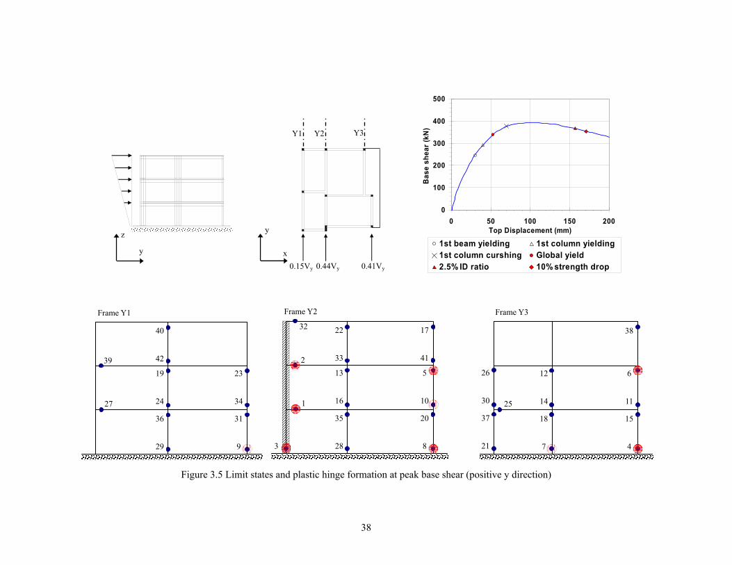
38

Figure 3.5 Limit states and plastic hinge formation at peak base shear (positive y direction)

x

y

0.15Vy 0.44Vy 0.41Vy

Y3 Y2 Y1

y

z 1st beam yielding 1st column yielding1st column curshing Global yield2.5% ID ratio 10% strength drop

0

100

200

300

400

500


Bas

e sh

ear (

kN)

12

14

18

7

6

11

15

4

25

38

26

30

37

21

Frame Y3

13

16

35

28

22

33

5

10

20

8

2

1

32 17

41

3

Frame Y2

19

24

36

29

40

42

23

34

31

9

39

27

Frame Y1

39

Figure 3.6 Limit states and plastic hinge formation at peak base shear (negative y direction)

x

y

0.15Vy 0.44Vy 0.41Vy

Y3Y2Y1y

z

0

100

200

300

400

500


Bas

e sh

ear (

kN)

1st beam yielding 1st column yielding1st column curshing Global yield2.5% ID ratio

2

14

7

4

11

17

28

16

44

10

19

21

8

9

20

Frame Y3

6

5

26

29

14

18

22

25

40

24

27

15

33

41

1

39

Frame Y2

12

13

30

23

32

37

34

38

45

31

43

36

46

35

42

Frame Y1

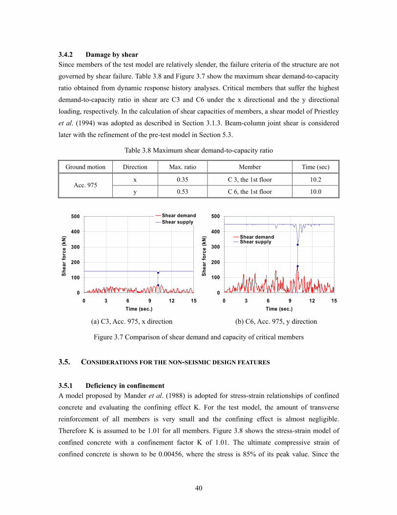
40

3.4.2 Damage by shear Since members of the test model are relatively slender, the failure criteria of the structure are not governed by shear failure. Table 3.8 and Figure 3.7 show the maximum shear demand-to-capacity ratio obtained from dynamic response history analyses. Critical members that suffer the highest demand-to-capacity ratio in shear are C3 and C6 under the x directional and the y directional loading, respectively. In the calculation of shear capacities of members, a shear model of Priestley et al. (1994) was adopted as described in Section 3.1.3. Beam-column joint shear is considered later with the refinement of the pre-test model in Section 5.3.

Table 3.8 Maximum shear demand-to-capacity ratio

Ground motion Direction Max. ratio Member Time (sec)

x 0.35 C 3, the 1st floor 10.2 Acc. 975

y 0.53 C 6, the 1st floor 10.0

0

100

200

300

400

500

0 3 6 9 12 15Time (sec.)

Shea

r for

ce (k

N)

Shear demandShear supply

0

100

200

300

400

500

0 3 6 9 12 15Time (sec.)

Shea

r for

ce (k

N) Shear demand

Shear supply

(a) C3, Acc. 975, x direction (b) C6, Acc. 975, y direction

Figure 3.7 Comparison of shear demand and capacity of critical members

3.5. CONSIDERATIONS FOR THE NON-SEISMIC DESIGN FEATURES

3.5.1 Deficiency in confinement A model proposed by Mander et al. (1988) is adopted for stress-strain relationships of confined concrete and evaluating the confining effect K. For the test model, the amount of transverse reinforcement of all members is very small and the confining effect is almost negligible. Therefore K is assumed to be 1.01 for all members. Figure 3.8 shows the stress-strain model of confined concrete with a confinement factor K of 1.01. The ultimate compressive strain of confined concrete is shown to be 0.00456, where the stress is 85% of its peak value. Since the

41

concrete model of Mander et al. (1988) was calibrated to the experimental data with higher confinement ratios, this model is not an accurate one for estimating ultimate strain of concrete with low confinement. Thus, it is expected that the ultimate strain of concrete with negligible confining effect is less than 0.00456 which is obtained from Mander et al. (1988) in Figure 3.8.

0

5

10

15

20

25

30

0 0.002 0.004 0.006 0.008 0.01strain

stre

ss (M

pa)

0.85 f'cc

εcu

Figure 3.8 Stress-strain model of confined concrete (Mander et al, 1988)

Judging from the previous discussion on ultimate strain of concrete, the constitutive model of concrete employed in ZeusNL may overestimate the capacity of real concrete with very little confinement. And unconfined parts of concrete members are also formulated by the model of Mander et al. (1988) by assuming the confinement factor K is 1.0. This material formulation in ZeusNL can accurately predict the stress-strain relationship of unconfined concrete when the strain ranges from zero to the value at peak stress. After the peak stress point, however, this model overestimates the capacity of unconfined concrete. Even in a very large strain range, the analytical model in ZeusNL assumes that cover concrete exists and has some parts of contribution to the member strength, which is not real. Therefore, at the extreme fiber of the core region, the strain obtained from ZeusNL is expected to be somewhat smaller than the real strain. For an axially loaded concrete test cylinder, its load-carrying capacity drops quickly after the peak and the ultimate strain is about 0.002-0.0025. In the latter case, all fibers in a section reach the ultimate strain and fail simultaneously. However, if a member is loaded in bending or bending and axial load, the section is subjected to a strain gradient, and the stress-strain curve drops gradually because of the re-distribution of strain upon attainment of peak strain in a fiber (MacGregor, 1997). This leads to the descending branch of the stress-strain curve after the maximum stress as shown in Figure 3.8. Therefore, the ultimate compressive strain of beams and eccentrically loaded columns is larger than that of concentrically loaded columns; 0.0038 is proposed by Hognestad (1951) and 0.0035 is proposed by the CEB-FIP Model Code-1990. Considering the fact that member modeling in ZeusNL can underestimate the real strain demand

42

of concrete members, it is desirable to use a value lower than 0.0038 suggested by Hognestad (1951) or 0.0035 suggested by the CEB-FIP Model Code-1990. Therefore, ultimate strain of compressive concrete for columns in this report is assumed to be 0.003.

3.5.2 Weak story Near collapse is indicated by a significant drop in stiffness, which proceeds collapse. In this situation, the story in question cannot support more lateral force. The formation of a weak story can be assessed by observing the change of story shear during the pushover analysis, as shown in Figure 3.9.

(a) Positive x direction (b) Positive y direction

Figure 3.9 Top displacement at C3 (the center column) versus story shear

Assuming that lateral force does not increase as the displacement increases, weak story behavior occurs when the capacity curve achieves a flat slope in Figure 3.9. Only the 1st story reaches the flat slope at its maximum strength, which is the same as base shear. Story shear values at other stories are lower than the base shear, and flat slope for those stories is achieved soon after the 1st story arrives at peak strength. The 1st story loses its strength ahead of the 2nd or the 3rd story failure and therefore the weak story is the 1st story. Because failure of the 1st story indicates total loss of strength for the whole structure, monitoring 1st story behavior can be a useful measure of critical limit states for the entire building.

3.5.3 Torsion An excitation given in only one direction leads to the responses of an asymmetric structure in both orthogonal directions and rotational, due to its coupled stiffness matrix. And this generates torsional responses in its fundamental mode shapes under dynamic loadings which cannot be captured by static analysis methods. Therefore estimation of torsion should be performed by dynamic response history analysis.

0

100

200

300

400

500

0 50 100 150 200Interstory drift (mm)

Stor

y sh

ear (

kN)


Top displacement (mm)

0

100

200

300

400

500

0 50 100 150 200Interstory drift (mm)

Stor

y sh

ear (

kN)


Top displacement (mm)

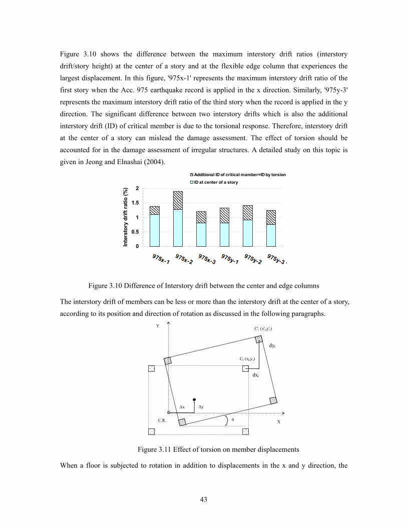
43

Figure 3.10 shows the difference between the maximum interstory drift ratios (interstory drift/story height) at the center of a story and at the flexible edge column that experiences the largest displacement. In this figure, '975x-1' represents the maximum interstory drift ratio of the first story when the Acc. 975 earthquake record is applied in the x direction. Similarly, '975y-3' represents the maximum interstory drift ratio of the third story when the record is applied in the y direction. The significant difference between two interstory drifts which is also the additional interstory drift (ID) of critical member is due to the torsional response. Therefore, interstory drift at the center of a story can mislead the damage assessment. The effect of torsion should be accounted for in the damage assessment of irregular structures. A detailed study on this topic is given in Jeong and Elnashai (2004).

0

0.5

1

1.5

2

975x-1975x-2

975x-3975z-1

975z-2975z-3

Inte

rsto

ry d

rift r

atio

(%)

Additional ID of critical mamber=ID by torsion

ID at center of a story

Figure 3.10 Difference of Interstory drift between the center and edge columns

The interstory drift of members can be less or more than the interstory drift at the center of a story, according to its position and direction of rotation as discussed in the following paragraphs.

θ

∆y ∆x

X

Y

Ci (xi,yi)

C'i (x'i,y'i)

C.R.

dyi

dxi

Figure 3.11 Effect of torsion on member displacements

When a floor is subjected to rotation in addition to displacements in the x and y direction, the

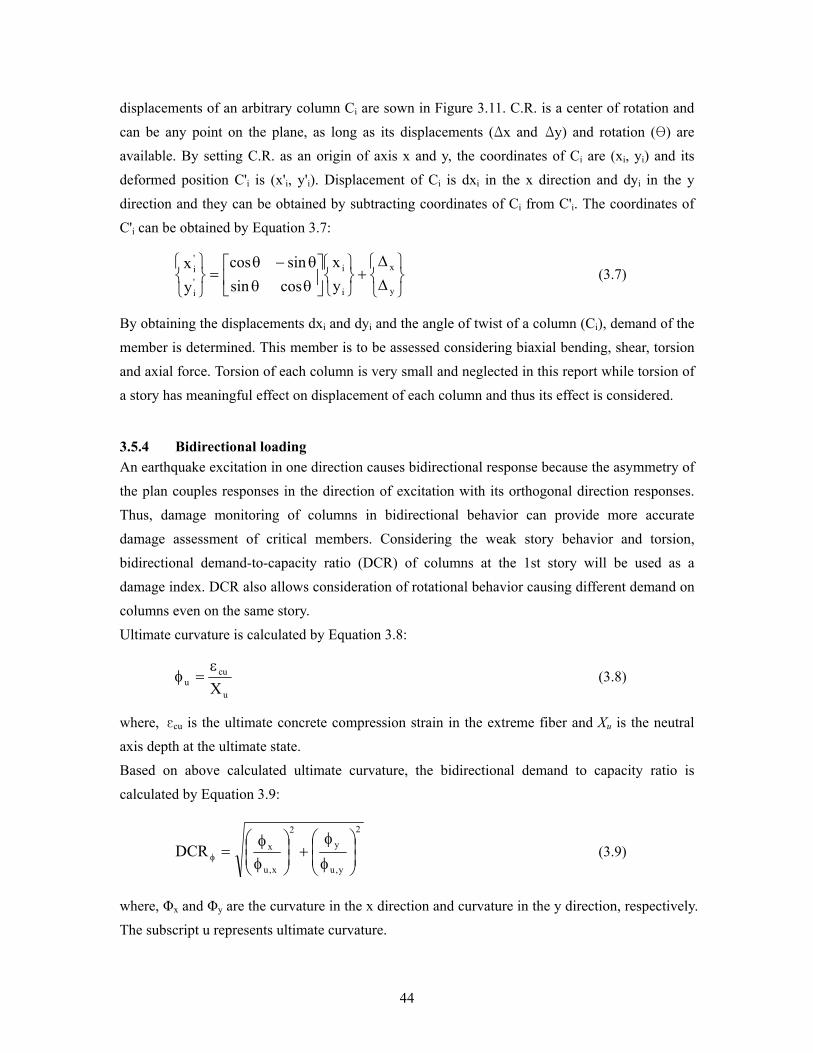
44

displacements of an arbitrary column Ci are sown in Figure 3.11. C.R. is a center of rotation and

can be any point on the plane, as long as its displacements (Δx and Δy) and rotation (θ) are available. By setting C.R. as an origin of axis x and y, the coordinates of Ci are (xi, yi) and its deformed position C'i is (x'i, y'i). Displacement of Ci is dxi in the x direction and dyi in the y direction and they can be obtained by subtracting coordinates of Ci from C'i. The coordinates of C'i can be obtained by Equation 3.7:

⎭⎬⎫

⎩⎨⎧

∆∆

+⎭⎬⎫

⎩⎨⎧

⎥⎦

⎤⎢⎣

⎡θθθ−θ

=⎭⎬⎫

⎩⎨⎧

y

x

i

i'i

'i

yx

cossinsincos

yx

(3.7)

By obtaining the displacements dxi and dyi and the angle of twist of a column (Ci), demand of the member is determined. This member is to be assessed considering biaxial bending, shear, torsion and axial force. Torsion of each column is very small and neglected in this report while torsion of a story has meaningful effect on displacement of each column and thus its effect is considered.

3.5.4 Bidirectional loading An earthquake excitation in one direction causes bidirectional response because the asymmetry of the plan couples responses in the direction of excitation with its orthogonal direction responses. Thus, damage monitoring of columns in bidirectional behavior can provide more accurate damage assessment of critical members. Considering the weak story behavior and torsion, bidirectional demand-to-capacity ratio (DCR) of columns at the 1st story will be used as a damage index. DCR also allows consideration of rotational behavior causing different demand on columns even on the same story. Ultimate curvature is calculated by Equation 3.8:

u

cuu X

ε=φ (3.8)

where, εcu is the ultimate concrete compression strain in the extreme fiber and Xu is the neutral axis depth at the ultimate state. Based on above calculated ultimate curvature, the bidirectional demand to capacity ratio is calculated by Equation 3.9:

2

y,u

y2

x,u

xDCR ⎟⎟⎠

⎞⎜⎜⎝

⎛

φ

φ+⎟

⎟⎠

⎞⎜⎜⎝

⎛

φφ

=φ (3.9)

where, Φx and Φy are the curvature in the x direction and curvature in the y direction, respectively. The subscript u represents ultimate curvature.

45

4. EARTHQUAKE SCENARIO FOR THE TEST

4.1. METHODOLOGY AND CRITERIA

Providing the most appropriate load condition for a full scale test which can be performed only once is an onerous task. In order to obtain comprehensive data for the investigation of the deficiencies of gravity load-designed buildings and its repair schemes, significant damage, without collapse, should be inflicted. For a systematic approach to deal with many scenarios of earthquakes, the procedure was divided into three steps followed by individual decision and reduction in the number of combinations. At first, an earthquake record was selected considering the possibility of collapse during the test. Then, intensity of the selected record was determined to obtain sufficient information on damage after the test. Finally, the direction of record was selected to achieve both collapse prevention and a severe damage level.

4.1.1 Ground motion records Through the discussion among partners of the SPEAR project, seven records in Table 4.1 were selected as candidates for the test record. Each of them is consist of two orthogonal components (Longitudinal and Translational) of horizontal accelerations and modified from natural records to be compatible to the EC8 Type 1 (for moderate or large events) design spectrum, soil type C (dense sand, gravel or stiff clay) and 5% damping. The latter records were normalized to peak ground acceleration (PGA) of 1.0g on rock site, which means that PGA is 1.15g on soil type C.

Table 4.1 List of semi-artificial records

No. Earthquakes Stations Components PGA (g)

1 Montenegro 1979 Ulcinj L, T 1.15

2 Montenegro 1979 Herceg Novi L, T 1.15

3 Friuli 1976 Tolmezzo L, T 1.15

4 Imperial Valley 1940 El Centro Array #9 L, T 1.15

5 Kalamata 1986 Prefecture L, T 1.15

6 Loma Prieta 1989 Capitola L, T 1.15

7 Imperial Valley 1979 Bonds Corner L, T 1.15

Elastic response spectra of the latter seven records in Table 4.1, after scaling down to 0.2g PGA, are presented in Appendix C with periods of the building.

46

4.1.2 Interstory drift as a damage index Figure 4.1 and Figure 4.2 show that excessive interstory drift at the weak story (the 1st story in the pre-test model with rigid links at column ends) causes failure of the test structure.

-200

-150

-100

-50

0

50

100

150

200

0 3 6 9 12 15Time (sec.)

Inte

rsto

ry d

rift i

n x

(mm

)


-200

-150

-100

-50

0

50

100

150

200

0 3 6 9 12 15Time (sec.)

Inte

rsto

ry d

rift i

n y

(mm

)


(a) Kalamata 1986 (Kalamata-Prefecture, 0.20g)

-200

-150

-100

-50

0

50

100

150

200

0 3 6 9 12 15Time (sec.)

Inte

rsto

ry d

rift i

n x

(mm

)


-200

-150

-100

-50

0

50

100

150

200

0 3 6 9 12 15Time (sec.)

Inte

rsto

ry d

rift i

n y

(mm

)1st level 2nd level 3rd level

(b) Kalamata 1986 (Kalamata-Prefecture, 0.25g)

-200

-150

-100

-50

0

50

100

150

200

0 3 6 9 12 15Time (sec.)

Inte

rsto

ry d

rift i

n x

(mm

)


-200

-150

-100

-50

0

50

100

150

200

0 3 6 9 12 15Time (sec.)

Inte

rsto

ry d

rift i

n y

(mm

)


(c) Kalamata 1986 (Kalamata-Prefecture, 0.3g)

Figure 4.1 Interstory drift time histories at C3 (Kalamata, bidirectional loading)

At the 1st story, large gravity load from the upper stories causes more P-delta effect than other

47

stories and reduction in capacities of columns as well. Thus the first story columns suffer much larger demand than other stories and interstory drift is a better indication of damage than top displacement.

Figure 4.2 Deformed shapes (at 4.64 sec. Kalamata, 0.2g, bidirectional loading)

A dynamic pushover analysis is assumed to be a better presentation of capacity because it can provide an appreciation of the difference caused by torsion and higher mode effects which are not presented by conventional pushover analysis. Comparisons are made between static pushover analysis and maximum responses from dynamic response history analyses in Figure 4.3, where #1 denotes unidirectional loading (either component L in the x direction or component T in the y direction) and #2 denotes bi-directional loading. The dynamic points are asynchronous peaks of base shear and roof displacement at the center column C3.

Montengro 1979_ Ulcinj2 #1 Montengro 1979_ Ulcinj2 #2Montengro 1979_ Herceg Novi #1 Montengro 1979_ Herceg Novi #2Friuli 1976_Tolmezzo #1 Friuli 1976_Tolmezzo #2Imperial Valley 1940_El Centro #1 Imperial Valley 1940_El Centro #2Kalamata_Prefecture #1 Kalamata_Prefecture #2Loma Prieta 1989_Capitola #1 Loma Prieta 1989_Capitola #2Imperial Valley 1979_Bonds Corner #1 Imperial Valley 1979_Bonds Corner #2Static pushover_positive Static pushover_negative

Figure 4.3 . Max. top displacement at C3 vs. max. base shear; (a) x direction, (b) y direction

y

0

100

200

300

400

500

0 50 100 150 200Max. top displacement in z (mm)

Max

. bas

e sh

ear i

n y

(kN

)

(b)

y

0

100

200

300

400

500

0 50 100 150 200Max. top displacement in x (mm)

Max

. bas

e sh

ear i

n x

(kN

)

(a)

48

Since viscous damping was not adopted in the dynamic analyses, the difference between the static pushover curve and maximum response points in Figure 4.3 is mainly caused by structural irregularities. Therefore, more careful investigation of capacities of the structure than provided by static pushover analysis is necessary for the assessment of an irregular building with unsymmetrical plans and a weak story.

4.1.3 Selection of ground motion All records in Table 4.1 were scaled down to make their peak ground acceleration (PGA) 0.2g and two orthogonal components were simultaneously applied to the analytical model. The results of static pushover analyses in Figure 2.8 imply that critical results will be obtained by applying ground motions to the structure in the weak axes. Therefore, L and T components of records were applied to the test building in the positive x and the positive y directions, respectively. The behavior of the building under the selected seven records is presented by interstory drift time histories as shown in Figure 4.4.

-120

-90

-60

-30

0

30

60

90

120

0 3 6 9 12 15Time (sec.)

Inte

rsto

ry d

rift i

n x

(mm

)


-120

-90

-60

-30

0

30

60

90

120

0 3 6 9 12 15Time (sec.)

Inte

rsto

ry d

rift i

n y

(mm

)


(a) Montenegro 1979 (Ulcinj2, 0.2g)

-120

-90

-60

-30

0

30

60

90

120

0 3 6 9 12 15Time (sec.)

Inte

rsto

ry d

rift i

n x

(mm

)


-120

-90

-60

-30

0

30

60

90

120

0 3 6 9 12 15Time (sec.)

Inte

rsto

ry d

rift i

n y

(mm

)


(b) Montenegro 1979 (Herceg Novi, 0.2g)

Figure 4.4 Interstory drift time histories at C3 in x and y directions

49

-120

-90

-60

-30

0

30

60

90

120

0 3 6 9 12 15Time (sec.)

Inte

rsto

ry d

rift i

n x

(mm


-120

-90

-60

-30

0

30

60

90

120

0 3 6 9 12 15Time (sec.)

Inte

rsto

ry d

rift i

n y

(mm

)


(c) Feiuli 1976 (Tolmezzo, 0.2g)

-120

-90

-60

-30

0

30

60

90

120

0 3 6 9 12 15Time (sec.)

Inte

rsto

ry d

rift i

n x

(mm

)


-120

-90

-60

-30

0

30

60

90

120

0 3 6 9 12 15Time (sec.)

Inte

rsto

ry d

rift i

n y

(mm

)


(d) Imperial Valley 1940 (El Centro Array #9, 0.2g)

-120

-90

-60

-30

0

30

60

90

120

0 3 6 9 12 15Time (sec.)

Inte

rsto

ry d

rift i

n x

(mm

)


-120

-90

-60

-30

0

30

60

90

120

0 3 6 9 12 15Time (sec.)

Inte

rsto

ry d

rift i

n y

(mm

)


(e) Kalamata 1986 (Kalamata-Prefecture, 0.2g)

Figure 4.4 Interstory drift time histories at C3 in x and y directions (continued)

50

-120

-90

-60

-30

0

30

60

90

120

0 3 6 9 12 15Time (sec.)

Inte

rsto

ry d

rift i

n x

(mm

)


-120

-90

-60

-30

0

30

60

90

120

0 3 6 9 12 15Time (sec.)

Inte

rsto

ry d

rift i

n y

(mm

)


(f) Loma Prieta 1989 (Capitola, 0.2g)

-120

-90

-60

-30

0

30

60

90

120

0 3 6 9 12 15Time (sec.)

Inte

rsto

ry d

rift i

n x

(mm

)


-120

-90

-60

-30

0

30

60

90

120

0 3 6 9 12 15Time (sec.)

Inte

rsto

ry d

rift i

n y

(mm

)


(g) Imperial Valley 1979 (Bonds Corner, 0.2g)

Figure 4.4 Interstory drift time histories at C3 in x and y directions (continued)

Failure prevention was considered as an important criterion for selection of a record to obtain more controllable results and a stream of good response data in the real test. After observation and comparison of analysis results in Figure 4.4, Montenegro 1979 (Herceg Novi) was selected because no pronounced peak was observed and the latter part of the response is lager than the earlier part, thus allowing considerable experimental results prior to subjecting the structure to the maximum demand region.

4.1.4 Intensity of ground motion for the test To determine an appropriate intensity of ground motion, damage levels of the structure under Montenegro 1979 (Herceg Novi) with various peak ground acceleration levels were investigated. The degree of damage was represented by the interstory drift demand-to-capacity ratio of critical columns as shown in Figure 4.5. As a damage index for preliminary selection of records, interstory drift was preferred to curvature because the former is easy to monitor and accurate

51

enough to estimate damage level on critical columns. The demand-to-capacity ratio of each column was calculated by Equation 4.1 in order to consider bi-directional behavior of the test building.

( ) ( )2y,uy

2x,ux //DCR ∆∆+∆∆=∆ (4.1)

where, ∆x and ∆x are the interstory drift in the x direction and in the y direction, respectively. The subscript u represents ultimate interstory drift. The ultimate interstory drift of each column in Table 4.2 is the column drift when its curvature reached the ultimate value under average axial force. The ultimate curvature is the curvature where the strain of core concrete is 0.003 or the strain tension steel is 0.1 and average axial force is calculated by static analysis with dead loads and 30% of live loads, excluding the effect of overturning moment under ground motions.

Table 4.2 Ultimate interstory drift (capacity) of each column at the 1st story

Ultimate interstory drift (mm) Location of columns

x y C1 36 36 C2 34 34 C3 26 26 C4 29 29 C5 78 78 C6 398* 38 C7 52 52 C8 88 88 C9 45 45

* represents failure of column is due to rupture of tension steel whose rupture strain is 0.1.

0

0.5

1

1.5

2

0 3 6 9 12 15Time (sec.)

Dem

and/

Cap

acity

(ID

)

C3 C1C2 C4

0

0.5

1

1.5

2

0 3 6 9 12 15Time (sec.)

Dem

and/

Cap

acity

(ID

)

C3 C1C2 C4

(a) Montenegro 1979 (Herceg Novi, 0.08g) (b) Montenegro 1979 (Herceg Novi, 0.10g)

Figure 4.5 DCR of critical columns, Montenegro 1979 - Herceg Novi

Center of rotation

y

x

C1 C2 C5

C3 C4 C9

C6 C7 C8

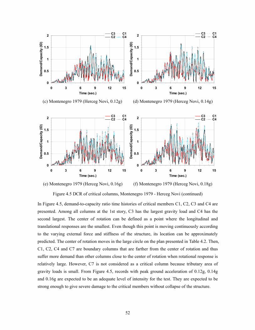
52

0

0.5

1

1.5

2

0 3 6 9 12 15Time (sec.)

Dem

and/

Cap

acity

(ID

)

C3 C1C2 C4

0

0.5

1

1.5

2

0 3 6 9 12 15Time (sec.)

Dem

and/

Cap

acity

(ID

)

C3 C1C2 C4

(c) Montenegro 1979 (Herceg Novi, 0.12g) (d) Montenegro 1979 (Herceg Novi, 0.14g)

0

0.5

1

1.5

2

0 3 6 9 12 15Time (sec.)

Dem

and/

Cap

acity

(ID

)

C3 C1C2 C4

0

0.5

1

1.5

2

0 3 6 9 12 15Time (sec.)

Dem

and/

Cap

acity

(ID

)

C3 C1C2 C4

(e) Montenegro 1979 (Herceg Novi, 0.16g) (f) Montenegro 1979 (Herceg Novi, 0.18g)

Figure 4.5 DCR of critical columns, Montenegro 1979 - Herceg Novi (continued)

In Figure 4.5, demand-to-capacity ratio time histories of critical members C1, C2, C3 and C4 are presented. Among all columns at the 1st story, C3 has the largest gravity load and C4 has the second largest. The center of rotation can be defined as a point where the longitudinal and translational responses are the smallest. Even though this point is moving continuously according to the varying external force and stiffness of the structure, its location can be approximately predicted. The center of rotation moves in the large circle on the plan presented in Table 4.2. Then, C1, C2, C4 and C7 are boundary columns that are farther from the center of rotation and thus suffer more demand than other columns close to the center of rotation when rotational response is relatively large. However, C7 is not considered as a critical column because tributary area of gravity loads is small. From Figure 4.5, records with peak ground acceleration of 0.12g, 0.14g and 0.16g are expected to be an adequate level of intensity for the test. They are expected to be strong enough to give severe damage to the critical members without collapse of the structure.

53

4.1.5 Direction of application of ground motion Collapse prevention and obtaining severe damage on critical members were used as criteria for selection of a record with its intensities in the previous sections. Two orthogonal components of the selected semi-artificial record, Montenegro 1979 (Herceg Novi) with peak ground acceleration (PGA) intensity of 1g are presented in Figure 4.6.

-1.5

-1

-0.5

0

0.5

1

1.5

0 3 6 9 12 15

Time (sec.)

Gro

und

acce

lera

tion

(g)

-1.5

-1

-0.5

0

0.5

1

1.5

0 3 6 9 12 15

Time (sec.)G

roun

d ac

cele

ratio

n (g

)

(a) Component L (b) Component T

Figure 4.6 Acceleration response history of Montenegro 1979 - Herceg Novi

After scaling down their PGA to 0.12g, 0.14g and 0.16g, they were applied to the building in eight different sets of directions as shown in Figure 4.7. Each combination of directions is defined as D1-D8, respectively.

Figure 4.7 Combinations of directions to apply ground motions

T y

x

C1 C2C5

C3 C4C9

C6 C7C8

L

L

L

L

T

T

TL

L

L

L

T

T

T

T

D1 D5 D6D2

D4 D8 D7D3

54

Torsion is an important characteristic in the seismic response of an asymmetric building and is considered as a main criterion for the decision of loading direction.

0

10

20

30

40

0 3 6 9 12 15Time (sec.)

Stan

dard

dev

iatio

n of

dem

and

D1 D2 D3 D4D5 D6 D7 D8

0

0.2

0.4

0.6

0.8

0 3 6 9 12 15Time (sec.)

Stan

dard

dev

iatio

n of

DC

R

D1 D2 D3 D4D5 D6 D7 D8

(a) Displacement demand (0.12g) (b) Demand-to-capacity ratio (0.12g)

0

10

20

30

40

0 3 6 9 12 15Time (sec.)

Stan

dard

dev

iatio

n of

dem

and

D1 D2 D3 D4D5 D6 D7 D8

0

0.2

0.4

0.6

0.8

0 3 6 9 12 15Time (sec.)

Stan

dard

dev

iatio

n of

DC

RD1 D2 D3 D4D5 D6 D7 D8

(c) Displacement demand (0.14g) (d) Demand-to-capacity ratio (0.14g)

0

10

20

30

40

0 3 6 9 12 15Time (sec.)

Stan

dard

dev

iatio

n of

dem

and

D1 D2 D3 D4D5 D6 D7 D8

0

0.2

0.4

0.6

0.8

0 3 6 9 12 15Time (sec.)

Stan

dard

dev

iatio

n of

DC

R

D1 D2 D3 D4D5 D6 D7 D8

(e) Displacement demand (0.16g) (f) Demand-to-capacity ratio (0.16g)

Figure 4.8 Standard deviation of column demands at the 1st story

55

Table 4.3 Two largest standard deviations of displacements and DCR of columns

Displacement DCR PGA (g)

1st 2nd 1st 2nd

0.12 D1 (28.1) D3 (26.2) D1 (0.54) D3 (0.49)

0.14 D1 (30.9) D3 (29.8) D7 (0.57) D1 (0.54)

0.16 D3 (30.7) D5 (27.8) D3 (0.58) D4 (0.56)

As shown in Figure 3.11, torsion causes different displacement demand according to the location of a column. This variation in demand can be conveniently appreciated by standard deviation of displacements of columns. Since standard deviation represents the sparseness of data, larger standard deviation of displacements of columns implies more effect of torsion. Comparing Figure 4.8 and angle of torsion time histories in Appendix D reveals standard deviation of column displacements can be a good measure of torsional effect. In order to see the effect of torsion in all cases of directional loading, standard deviation of displacements and bidirectional demand-to-capacity ratios of columns are presented in Figure 4.8. The two largest values and corresponding directions of loadings are summarized in Table 4.3. Figure 4.8 and Table 4.3 shows that loading cases where the effect of torsion is the largest are 0.12g-D1, 0.14g-D1 and 0.16g-D3 (intensity-direction). As an expansion of response monitoring methods used in previous steps of deciding record and intensity, interstory drift and DCR of critical members with various intensities and directions of loading are presented in Appendix E and Appendix F, respectively.

4.2. BEHAVIOR AND DAMAGE ESTIMATIOIN

In previous sections, Montenegro 1979 (Herceg Novi) is used as the test record and the number of candidates for the earthquake scenario is reduced to three: (i) 0.12g-D1, (ii) 0.14g-D1 and (iii) 0.16g-D3. In order to choose one earthquake scenario, these three candidates are to be carefully investigated by damage assessment through curvature DCR of each critical member.

4.2.1 Damage expectation and selection of a scenario For the accurate damage monitoring, bidirectional curvature ductility demand-to-capacity ratio for the 1st story columns are calculated. Ultimate curvature of each column is obtained by Equation 3.8 which is presented again below.

u

cuu X

ε=φ

In using this equation, ultimate compressive strain of concrete is assumed to be 0.003, as explained in section 3.5.1. Then bidirectional demand-to-capacity ratio (DCR) is calculated by

56

Equation 4.2 which is presented below.

2

y,u

y2

x,u

xDCR ⎟⎟⎠

⎞⎜⎜⎝

⎛

φ

φ+⎟

⎟⎠

⎞⎜⎜⎝

⎛

φφ

=φ (4.2)

Table 4.4 shows the bidirectional demand-to-capacity ratios when the displacement demands at the 1st story columns are critical. For comparison, various demand-to-capacity ratios are

calculated based on other ultimate strains of concrete in addition to 0.003. 0.0035 is the value proposed by CEB-FIP Model Code-1990 and 0.00456 is the ultimate strain calculated by Mander's stress-strain model for confined concrete with K=1.01. Shaded results in Table 4.4 are

demand-to-capacity ratios when ultimate strain of concrete is 0.003. The results in Table 4.4 are also presented in Figure 4.9. From the latter figure, it is clear that gravity load and torsion have great influence on the DCR.

Table 4.4 Bidirectional curvature demand-to-capacity ratio of columns

Montenegro 1979 - Herceg Novi Scenario 0.12g-D1 (at 8.10 sec.) 0.14g-D1 (at 8.20 sec.) 0.16g-D3 (at 11.15 sec.)

εcu(1E-3) 3 3.5 4.56 3 3.5 4.56 3 3.5 4.56 C1 1.16 0.98 0.75 1.32 1.11 0.84 0.27 0.22 0.17 C2 2.00 1.73 1.32 2.19 1.90 1.44 1.11 0.97 0.73 C3 0.33 0.27 0.21 0.39 0.33 0.25 0.85 0.72 0.54 C4 1.50 1.23 0.97 1.54 1.27 0.99 1.38 1.13 0.89 C5 0.41 0.34 0.27 0.46 0.39 0.30 0.05 0.05 0.04 C6 0.30 0.25 0.18 0.37 0.31 0.23 0.26 0.22 0.16 C7 0.61 0.51 0.39 0.61 0.51 0.39 0.74 0.61 0.47 C8 0.20 0.16 0.13 0.25 0.21 0.16 0.43 0.36 0.27 C9 0.10 0.08 0.06 0.09 0.08 0.06 0.54 0.45 0.35

From Table 4.4 and Figure 4.9, it is observed that Montenegro 1979 (Herceg Novi) record at 0.12g PGA in the direction D1 leads to severe damage on C1, C2 and C4 due to torsion but the damage level on C3 is low. A large variation in damage level on columns implies that the effect of torsion is significant. Less damage on C3 means lower possibility of collapse during the test and thus leads to obtaining comprehensive test data. Therefore, Montenegro 1979 (Herceg Novi) record at 0.12g PGA in the direction D1 can be suggested as an appropriate earthquake scenario for the test. Considering that the ultimate capacities of critical members are conservatively assumed in this report, 0.12g PGA is expected to be a lower bound of appropriate levels of intensity for the test. Thus, higher intensity in Table 4.4 such as 0.14g or 0.16g may be determined as the appropriate level through the discussion among partners.

57

(c) PGA-0.16g, direction-D3

y

x

C1 C2C5

C3 C4C9

C6C8

[0.05] [0.27] [1.11]

[0.85]

[1.38]

[0.26] C7

[0.74]

[0.54]

[0.43]

(b) PGA-0.14g, direction-D1

y

x

C1 C2C5

C3 C4C9

C6C8

[0.46] [1.32] [2.19]

[0.39]

[1.54]

[0.37] C7

[0.61]

[0.09]

[0.25]

(a) PGA-0.12g, direction-D1

y

x

C1 C2C5

C3 C4C9

C6C8

[0.41] [1.16] [2.00]

[0.33]

[1.50]

[0.30] C7

[0.61]

[0.10]

[0.20]

Column ID.

Max. curvature demand-to-capacity ratio

Figure 4.9 Curvature demand-to-capacity ratio of columns

58

4.2.2 Displacement information for the test setup For an investigation on responses of the test building under the selected record, top displacement, interstory drift ratio (interstory drift/story height) at the center column (C3) and base shear time histories are presented in Figure 4.10.

-100-80-60-40-20

020406080

100

0 3 6 9 12 15

Time (sec.)

Top

disp

lace

men

t (m

m)

-100-80-60-40-20

020406080

100

0 3 6 9 12 15

Time (sec.)

Top

disp

lace

men

t (m

m)

(a) Top displacement at C3 (x) (b) Top displacement at C3 (y)

-1.5

-1

-0.5

0

0.5

1

1.5

0 3 6 9 12 15

Time (sec.)

Inte

rsto

ry d

rift r

atio

(%)


-1.5

-1

-0.5

0

0.5

1

1.5

0 3 6 9 12 15

Time (sec.)

Inte

rsto

ry d

rift r

atio

(%)


(c) Interstory drift ratio at C3 (x) (d) Interstory drift ratio at C3 (y)

-400

-200

0

200

400

0 3 6 9 12 15

Time (sec.)

Bas

e sh

ear (

kN)

-400

-200

0

200

400

0 3 6 9 12 15

Time (sec.)

Bas

e sh

ear (

kN)

(e) Base shear (x) (f) Base shear (y)

Figure 4.10 Montenegro 1979 (Herceg Novi, 0.12g), D1

59

5. REFINEMENT OF THE PRE-TEST ANALYTICAL MODELING

At the final stage of the test setup, fully detailed information on the test structure became available and the pre-test analytical model was refined according to this additional information. More sophisticated analytical models were generated by implementing actual material properties, rigid diaphragm for slab floors and shear deformation modeling of beam-column joints.

5.1. MATERIAL PROPERTIES UPDATE

Experimental testing of concrete and reinforcing steel that were sampled at ELSA during the construction of the test structure provided properties of actual materials which are exactly same as those used in the real structure. These actual material properties are adopted in the refined analytical model, while assumed material properties in Section 2.2.3 had been used before the test of actual materials. The values of actual material properties are compared with their designed and assumed values in Table 5.1 and Figure 5.1.

Table 5.1 Designed, assumed and actual material properties

Concrete Steel

Member Designed f'c (MPa)

Assumed f'c (MPa)

Actual f'c (MPa)

Bar size

Designed Fy (MPa)

Assumed Fy (MPa)

Actual Fy (MPa)

1st FL. column 25 25 24.73 1st FL. slab 25 25 26.7

8mm 220 467 479

2nd FL. column 25 25 26.7 2nd FL. slab 25 25 27.53

12mm 360 459 474

3rd FL. column 25 25 25.32 3rd FL. slab 25 25 27.39

20mm 360 377 397

0

5

10

15

20

25

30

f'c (M

Pa)

Designed Assumed Actual

1st FL. col. 1st FL. slab 2nd FL. col. 2nd FL. slab 3rd FL. col. 3rd FL. slab0

100

200

300

400

500

Fy (M

Pa)

Designed Assumed Actual

8mm 12mm 20mm

(a) Compressive strength (f'c) of concrete (b) Yield strength (Fy) of steel

Figure 5.1 Comparison of material properties

The assumed values of Fy were obtained from material samples of steel industries, while the samples for actual Fy were obtained from the test structure. The assumed or actual yield strength

60

is higher than its original design in Section 2.2.1 because the steel industry does not produce low strength steel in early 70's any longer. In the final refinement of the analytical modeling, the actual Fy values which were obtained directly from construction materials were used. Figure 5.2 shows comparison of capacities of the pre-test models with material properties in Table 5.1. The difference between steel strengths of designed and actual material properties caused the large difference between the corresponding capacity curves in Figure 5.2.

0

100

200

300

400

500

0 50 100 150 200Top displacement in x (mm)

Bas

e sh

ear i

n x

(kN

)

Actual material propertiesAssumed material propertiesDesigned material properties

0

100

200

300

400

500

0 50 100 150 200Top displacement in y (mm)

Bas

e sh

ear i

n y

(kN

)

Actual material propertiesAssumed material propertiesDesigned material properties


Figure 5.2 Capacity comparison of models with different material properties

5.2. RIGID DIAPHRAGM MODELING OF FLOOR SLABS

At each floor, four actuator mounting blocks and two pairs of connecting elements were monolithically constructed with the floor slab as shown in Figure 5.3.

(a) Drawing of actuator mounting blocks (b) Construction of actuator mounting blocks

Figure 5.3 Actuator connecting elements on slabs

61

Figure 5.3 shows that the mounting blocks are highly reinforced and fastened to each other by connecting elements in which prestressing bars (DYWDAG Ф 36 mm) are embedded. This situation ensures good load transferring conditions from loading pistons to the test structure and provides much higher stiffness against horizontal twist to the floor slab than its original modeling (Figure 5.4 (a)) which is presented in Section 2.2. Thus implementation of rigid diaphragm of floor slabs became necessary for more accurate analytical modeling. In order to model slabs as rigid diaphragms, each corner of a slab is diagonally connected to the opposite corner as shown in Figure 5.4 (b).

(a) 3D model without rigid diaphragm (b) 3D model with rigid diaphragm

(c) Section of horizontally rigid member

Figure 5.4 Rigid diaphragms in 3D analytical modeling

The dimensions and reinforcement of connecting members for the rigid diaphragm modeling were determined for the additional members not to provide duplicated stiffness to the flexural behavior of beams, because the contribution of slabs to flexural stiffness of beams is already modeled by effective width of T-beam models. The thickness of the connecting elements was determined by iterating it such that the contribution of connecting elements to the vertical stiffness is negligible, while the contribution to the horizontal stiffness remains huge. As shown in Figure 5.4 (c), the thin section of the connecting members and single-layered reinforcement present only horizontal stiffness to the floor without vertically stiffening the adjacent beams.

1000 mm

15 mm

Concrete (f'c=26.7MPa)

Steel (fy=474MPa)

As=100 mm2

As=50 mm2

62

Figure 5.5 represents the angle of torsion at all corners of slabs that are located at column points. The analytical model with additional connecting members (Figure 5.5 (b)) shows the same angle of torsion at every corner and this behavior satisfies the assumption of slab diaphragm.

-9

-6

-3

0

3

6

9

0 5 10 15Time (sec.)

Ang

le o

f tor

sion

(E-3

rad)

-9

-6

-3

0

3

6

9

0 5 10 15Time (sec.)

Ang

le o

f tor

sion

(E-3

rad)

(a) Without rigid diaphragm in slap modeling (b) With diaphragm in slab modeling

Figure 5.5 Angle of torsion time histories at all columns in the 1st story (Montenegro 1979 - Herceg

Novi, 0.2g, bidirectional loading)

5.3. MODELING OF BEAM-COLUMN CONNECTIONS

5.3.1 Shear deformation modeling of RC beam-column connections According to the detailed construction drawings and figures of the SPEAR test structure, stirrups do not continue in the beam-column connections. This type of beam-column connection detail increases the probability of joint shear failure under earthquake loadings. Therefore, joint elements that represent shear deformation of beam-column connections were implemented into the pre-test analytical model. The shear strain-stress relationship is assumed to be tri-linear, as shown in Figure 5.6. Parameters to define the tri-linear model are explained in Table 5.2 and methods to obtain shear strength and stiffness of beam-column connections are represented in Section 5.3.1.1 and 5.3.1.2.

Figure 5.6 Tri-linear shear stress-strain relationship

0

1

2

3

4

0 0.5 1 1.5Shear strain (1E-3 rad)

Shea

r stre

ss (M

pa)

τp

τc

k2

k1

63

Table 5.2 Parameters for the shear stress-strain relationship

Parameters Descriptions

τc Shear stress at cracking (MPa) Strength

τp Shear stress at maximum capacity (MPa)

k1 Stiffness up to cracking (MPa) = G (Shear modulus of elasticity) Stiffness

k2 Stiffness between cracking and maximum capacity (MPa)

5.3.1.1. Shear strength estimation In order to estimate appropriate shear strength of beam-column joints, various references were reviewed and compared, as shown in Table 5.3, Table 5.4 and Figure 5.8. FEMA 356 (2001) presents shear capacity of RC beam-column connections in various situations of adjacent members and all range of transverse steel ratios. In this report, therefore, FEMA 356 (2001) was utilized in calculating the shear stress at maximum capacity. Cracking stress and stiffness are calculated by using the nonlinear section analysis program 'Response 2000' by Bentz (2000) and test data from Walker (2001), as represented in Table 5.5.

Table 5.3 References for estimating joint shear capacity

References Comments

ACI 318 This provision overestimates the shear capacity by assuming that beam-column

joint has minimum amount of transverse reinforcement.

FEMA 356 The case of low transverse steel ratio (less than 0.3%) is applicable to SPEAR

frame.

Response 2000

-Bentz (2000)

This program underestimates the shear capacity because confinement effect by

adjacent members cannot be modeled.

Calvi et al. 2002

Joints tested in this paper do not have transverse beams and thus are weaker than

those of the SPEAR frame. Though the test was conducted with interior joint,

exterior joint and knee joint, only the sub-assembly with external joint failed due

to joint capacity limitation. Only the strength of interior joint is available.

Walker 2001 Only the internal joint case was tested.

The joint shear strength can be calculated by Equation 5.1 (ACI 318):

j'cjj AfV ⋅⋅γ= (5.1)

where Vj is the nominal joint shear force in lb, γj is the joint shear factor, fc' is the compressive

strength of concrete in psi and Aj is the effective horizontal joint area in in2. For beam-column

64

joints, the nominal cross-sectional area, Aj, is defined by a joint depth equal to the column dimension in the direction of framing and a joint width equal to the smallest of (i) the column width, (ii) the beam width plus the joint depth and (iii) twice the smaller perpendicular distance from the longitudinal axis of the beam to the column side (FEMA 356, 2001). The effective horizontal joint area Aj of column C6 is conservatively calculated by excluding the part of which the surface is not faced to the adjacent beams, as shown in Figure 5.7.

Figure 5.7 Locations of beam-column joints

In order to compare shear capacities from various references, shear strength factor defined in Equation 5.2 is utilized. This factor is normalized by cross sectional area and compressive strength of concrete

j

'c

jj

Af

V

⋅=γ (5.2)

0

5

10

15

20

25

0 5 10 15 20 25 30Column #

Shea

r stre

ngth

fact

ors

ACI 318FEMA 356Response 2000Calvi et al. 2002Walker 2001

0

5

10

15

20

25

0 5 10 15 20 25 30Column #

Shea

r stre

ngth

fact

ors

ACI 318FEMA 356Response 2000Calvi et al. 2002Walker 2001


Figure 5.8 Comparison of shear strength factors (Column #: 1st story: 1~9, 2nd story: 11~19, 3rd story: 21~29; the ones place digits represent column numbers in Figure 5.7)

B5

B6

C6_i

C6_o

y

x

C1 C2C5

C3 C4 C9

C6 C7 C8

65

The maximum shear strength is estimated according to FEMA 356 as shown in Table 5.4.

Table 5.4 Comparison of shear strength factors (γj)

ACI 318 FEMA 356 Response 2000 Calvi et al. 2002 Walker 2001 Joint locations

x y x y x y x y x y

C1 20.0 15.0 10.0 8.0 4.3 4.3 - - 11.4 -

C2 15.0 15.0 6.0 6.0 4.4 4.4 3.7 3.7 - -

C3 15.0 20.0 8.0 12.0 5.4 5.4 - - - 11.4

C4 15.0 15.0 6.0 6.0 4.9 4.9 3.7 3.7 - -

C5 15.0 15.0 6.0 6.0 3.4 3.4 3.7 3.7 - -

C6_i 15.0 20.0 8.0 10.0 3.3 3.3 - - - -

C6_o 15.0 15.0 6.0 6.0 3.3 3.3

C7 15.0 15.0 6.0 6.0 3.8 3.8 3.7 3.7 - -

C8 15.0 15.0 6.0 6.0 3.3 3.3 3.7 3.7 - -

1st

story

C9 15.0 20.0 8.0 10.0 4.0 4.0 - - - 11.4

C1 20.0 15.0 10.0 8.0 3.7 3.7 - - - -

C2 15.0 15.0 6.0 6.0 3.7 3.7 3.7 3.7 - -

C3 20.0 20.0 8.0 12.0 4.4 4.4 - - - 11.4

C4 15.0 15.0 6.0 6.0 4.0 4.0 3.7 3.7 - -

C5 15.0 15.0 6.0 6.0 3.1 3.1 3.7 3.7 - -

C6_i 15.0 20.0 8.0 10.0 3.0 3.0 - - - -

C6_o 15.0 15.0 6.0 6.0 3.0 3.0

C7 15.0 15.0 6.0 6.0 3.3 3.3 3.7 3.7 - -

C8 15.0 15.0 6.0 6.0 3.0 3.0 3.7 3.7 - -

2nd

story

C9 15.0 20.0 8.0 10.0 3.5 3.5 - - - 11.4

C1 15.0 12.0 10.0 4.0 3.1 3.1 - - - -

C2 12.0 12.0 4.0 4.0 3.1 3.1 - - - -

C3 15.0 15.0 4.0 8.0 3.3 3.3 - - - -

C4 12.0 12.0 4.0 4.0 3.2 3.2 - - - -

C5 12.0 12.0 4.0 4.0 2.9 2.9 - - - -

C6_i 12.0 15.0 4.0 10.0 2.9 2.9 - - - -

C6_o 12.0 12.0 4.0 4.0 2.9 2.9 - -

C7 12.0 12.0 4.0 4.0 2.9 2.9 3.7 3.7 - -

C8 12.0 12.0 4.0 4.0 2.8 2.8 - - - -

3rd

story

C9 12.0 15.0 4.0 10.0 3.0 3.0 3.7 3.7 - -

66

5.3.1.2. Shear stiffness estimation The average stiffness before cracking (k1) obtained from analytical models of 'Response 2000' (R-2000) is 8587.7 Mpa. This value is similar to the G (shear modulus of elasticity) of concrete calculated by Equation 5.3.

Mpa8333)2.01(2

20000)1(2

EG =+

=ν+

=γτ

= (5.3)

In calculating G by Equation 5.3, it is assumed that the material is normal weight concrete and its Young's modulus Ec ≈ 20000 Mpa and Poisson's ratio ν ≈ 0.2. The shear stiffness after cracking (k2) is estimated from the relationship between maximum shear strength (τp) and shear strain at maximum strength (dp), as shown in Equation 5.4.

cp

cp2 dd

k−

τ−τ= (5.4)

where, the shear strain at cracking (dc) is calculated by dc= τp/k1. Cracking shear stresses (τc) and shear strain at maximum strengths (dp) for 'knee joint' and 'internal joint without transverse beams' are obtained from 'Response 2000' simulation and experimental data from Walker (2001). Cracking strength and stiffness of other joint types are calculated by interpolating or extrapolating the values of 'Knee joint' and 'Internal joint w/o transverse beams' which are known by 'Response 2000' simulation and experimental data from Walker (2001), respectively, as shown in Table 5.5.

Table 5.5 Parameters of shear stress-strain relationship according to joint types

Shear strength factor (γj) Initial stiffness Shear strain at τp No. Joint type

Cracking point Max. point k1 (Mpa) dp (radian)

1 Knee joint 4 (R-2000) 4 (FEMA356) 8587.7 (R-2000) 0.0002 (R-2000)

2 External joint w/o

transverse beams 4.5 6 (FEMA356) 8587.7 0.0018

3 External joint w/

transverse beams 5 8 (FEMA356) 8587.7 0.0034

4 Internal joint w/o

transverse beams 5.5 (Walker, 2001) 10 (FEMA356) 8587.7 0.005 (Walker, 2001)

5 Internal joint w/

transverse beams 6 12 (FEMA356) 8587.7 0.0066

The post-cracking shear stiffness of each beam-column joint is represented in Table 5.6. The joint type numbers in the latter table are same as the numbers in Table 5.5. The location of beam-

67

column joints of the test model is expressed in the format of 'column number_story (direction)'. For example, 'C1_3(y)' is a joint behavior at the top of column C1 on the 3rd story in the y direction.

Table 5.6 Shear stiffness of beam-column joints

Joint type Joint locations in the SPEAR frame k1 (Mpa) k2 (Mpa)

No 1 C1_3(y), C2_3(x), C2_3(y), C3_3(x), C4_3(x), C4_3(y), C5_3(x), C5_3(y),

C6i_3(x), C6o_3(x), C6o_3(y), C7_3(x), C7_3(y), C8_3(x), C8_3(y), C9_3(x) 8587.7 0

No 2

C2_1(x), C2_1(y), C4_1(x), C4_1(y), C5_1(x), C5_1(y), C6o_1(x), C6o_1(y),

C7_1(x), C7_1(y), C8_1(x), C8_1(y), C2_2(x), C2_2(y), C4_2(x), C4_2(y), C5_2(x),

C5_2(y), C6o_2(x), C6o_2(y), C7_2(x), C7_2(y), C8_2(x), C8_2(y)

8587.7 393.5

No 3 C1_1(y), C3_1(x), C6i_1(x), C9_1(x), C1_2(y), C3_2(x), C6i_2(x), C9_2(x),

C3_3(y) 8587.7 394.4

No 4 C1_1(x), C6i_1(y), C9_1(y), C1_2(x), C6i_2(y), C9_2(y), C1_3(x), C6i_3(y),

C9_3(y) 8587.7 394.6

No 5 C3_1(y), C3_2(y) 8587.7 394.8

Shear strength-strain relationships of five types of beam-column joints defined in Table 5.5 and Table 5.6 are presented in Figure 5.9.

0

2

4

6

8

10

12

14

0 0.002 0.004 0.006 0.008 0.01Shear strain (rad)

Shea

r stre

ss fa

ctor

No1 No2 No3 No4 No5

Figure 5.9 Shear strength-strain relationships

5.3.2 Response of beam-column connections Detailed responses of the 1st story beam-column connections and locations of critical connections under the Montenegro 1979 record (Herceg Novi, 0.15g, bidirectional loading, D1) are shown in Figure 5.10 and Figure 5.11. From the latter figures, the probability of shear failure is the highest at beam-column connection of C4.

68

-200

-150

-100

-50

0

50

100

150

200

-12 -6 0 6 12Rotation (E-6 rad.)

Mom

ent (

kN-m

)

-200

-150

-100

-50

0

50

100

150

200

-12 -6 0 6 12Rotation (E-6 rad.)

Mom

ent (

kN-m

)

-200

-150

-100

-50

0

50

100

150

200

-12 -6 0 6 12Rotation (E-6 rad.)

Mom

ent (

kN-m

)

C1 C2 C3

-200

-150

-100

-50

0

50

100

150

200

-12 -6 0 6 12Rotation (E-6 rad.)

Mom

ent (

kN-m

)

-200

-150

-100

-50

0

50

100

150

200

-12 -6 0 6 12Rotation (E-6 rad.)

Mom

ent (

kN-m

)

-200

-150

-100

-50

0

50

100

150

200

-12 -6 0 6 12Rotation (E-6 rad.)

Mom

ent (

kN-m

)

C4 C5 C6

-200

-150

-100

-50

0

50

100

150

200

-12 -6 0 6 12Rotation (E-6 rad.)

Mom

ent (

kN-m

)

-200

-150

-100

-50

0

50

100

150

200

-12 -6 0 6 12Rotation (E-6 rad.)

Mom

ent (

kN-m

)

-200

-150

-100

-50

0

50

100

150

200

-12 -6 0 6 12Rotation (E-6 rad.)

Mom

ent (

kN-m

)

C7 C8 C9

Figure 5.10 Beam-column joint deformations and locations of critical beam-column connections on the plan of the test structure (x direction shear displacement, rotation about y axis), Montenegro 1979 - Herceg Novi, 0.15g, bidirectional loading

* The large arrows indicate the locations of critical connections where the shear forces are larger than shear strengths (τp).

z

x

B1

B1 B2

B3 B4

B5 B6

B1 B8

B9 B7 B1

C1 C2 C5

C3 C4 C9

C6 C7 C8 y

69

-200-150-100

-500

50100150200

-12 -6 0 6 12Rotation (E-6 rad.)

Mom

ent (

kN-m

)

-200

-150

-100

-50

0

50

100

150

200

-12 -6 0 6 12Rotation (E-6 rad.)

Mom

ent (

kN-m

)

-200

-150

-100

-50

0

50

100

150

200

-12 -6 0 6 12Rotation (E-6 rad.)

Mom

ent (

kN-m

)

C1 C2 C3

-200

-150

-100

-50

0

50

100

150

200

-12 -6 0 6 12Rotation (E-6 rad.)

Mom

ent (

kN-m

)

-200

-150

-100

-50

0

50

100

150

200

-12 -6 0 6 12Rotation (E-6 rad.)

Mom

ent (

kN-m

)

-200

-150

-100

-50

0

50

100

150

200

-12 -6 0 6 12Rotation (E-6 rad.)

Mom

ent (

kN-m

)

C4 C5 C6

-200

-150

-100

-50

0

50

100

150

200

-12 -6 0 6 12Rotation (E-6 rad.)

Mom

ent (

kN-m

)

-200

-150

-100

-50

0

50

100

150

200

-12 -6 0 6 12Rotation (E-6 rad.)

Mom

ent (

kN-m

)

-200

-150

-100

-50

0

50

100

150

200

-12 -6 0 6 12Rotation (E-6 rad.)

Mom

ent (

kN-m

)

C7 C8 C9

Figure 5.11 Beam-column joint deformations and locations of critical beam-column connections on the plan of the test structure (y direction shear displacement, rotation about x axis), Montenegro 1979 - Herceg Novi, 0.15g, bidirectional loading

* The large arrows indicate the locations of critical connections where the shear forces are larger than shear strengths (τp).

z

x

B1

B1 B2

B3 B4

B5 B6

B1 B8

B9 B7 B1

C1 C2 C5

C3 C4 C9

C6 C7 C8 y

70

5.4. COMPARISON OF RESPONSES OF PRE-TEST ANALYTICAL MODELS

Pre-test analytical models and their modeling options are represented in Table 5.7. The parametric value of each modeling option was determined by discussions in previous sections 2.2.2, 5.2 and 5.3. The difficulties in the prediction of beam-column connection behavior of RC structures left the use of 'rigid links at column ends' and 'beam-column joint shear' selective, while 'slab rigid diaphragm' was adopted by all pre-test models.

Table 5.7 Pre-test analytical models

Slab rigid diaphragm Rigid links at column ends Beam-column joint shear Model #1 Yes No No Model #2 Yes Yes No Model #3 Yes No Yes Model #4 Yes Yes Yes

Capacity curves and dynamic response histories are compared in Figure 5.12 and Figure 5.13, respectively.

0

100

200

300

400

500

-200 -100 0 100 200

Top displacement in x (mm)

Bas

e sh

ear i

n x

(kN

)

Model #1Model #2Model #3Model #4

0

100

200

300

400

500

-200 -100 0 100 200

Top displacement in z (mm)

Bas

e sh

ear i

n y

(kN

)

Model #1Model #2Model #3Model #4

(a) x direction (b) y direction Figure 5.12 Comparison of capacity curves

-90

-60

-30

0

30

60

90

0 3 6 9 12 15Time (sec.)

Top

disp

l in

x (m

m)

Model #1 Model #2Model #3 Model #4

-90

-60

-30

0

30

60

90

0 3 6 9 12 15Time (sec.)

Top

disp

l in

y (m

m)

Model #1 Model #2Model #3 Model #4

(a) Top displacement in x direction (b) Top displacement in y direction Figure 5.13 Comparison of response histories at the center column (C3), Montenegro 1979 - Herceg Novi, 0.15g, bidirectional loading

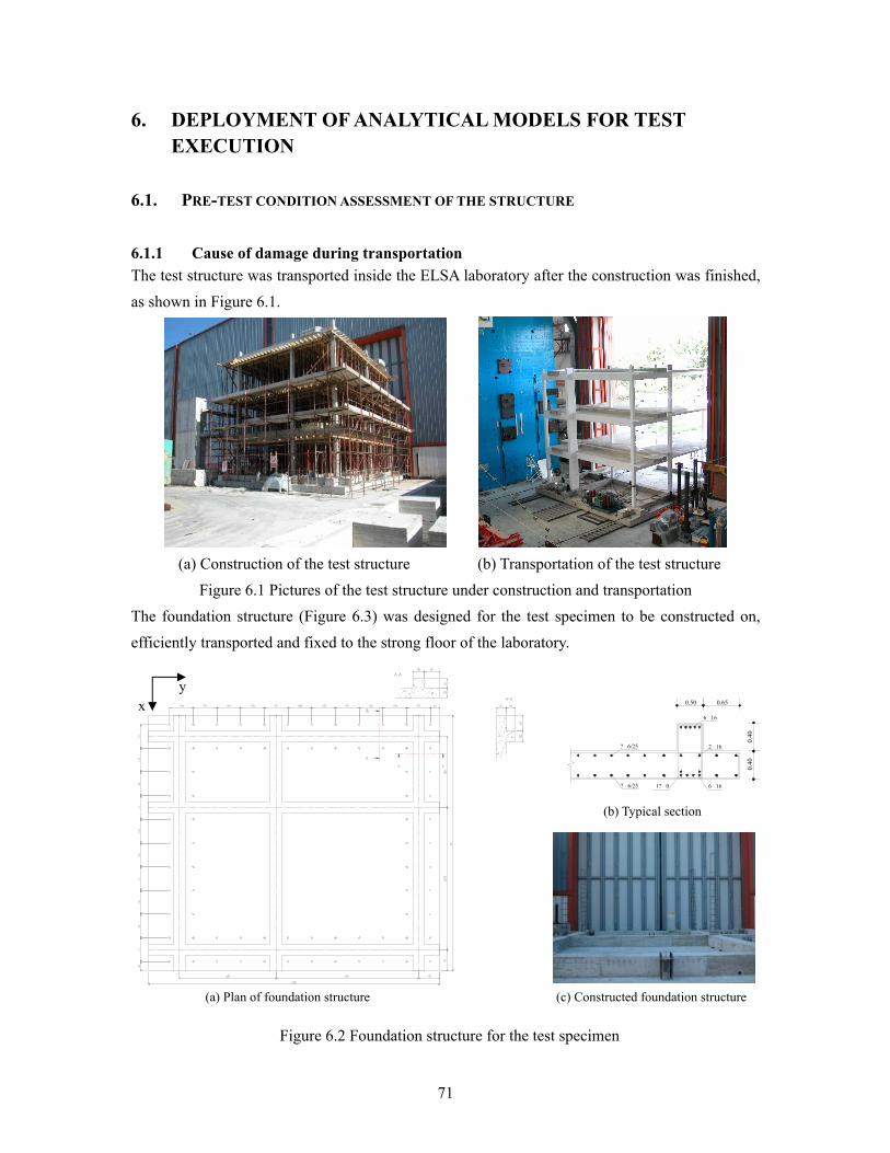
71

6. DEPLOYMENT OF ANALYTICAL MODELS FOR TEST EXECUTION

6.1. PRE-TEST CONDITION ASSESSMENT OF THE STRUCTURE

6.1.1 Cause of damage during transportation The test structure was transported inside the ELSA laboratory after the construction was finished, as shown in Figure 6.1.

(a) Construction of the test structure (b) Transportation of the test structure

Figure 6.1 Pictures of the test structure under construction and transportation The foundation structure (Figure 6.3) was designed for the test specimen to be constructed on, efficiently transported and fixed to the strong floor of the laboratory.

Figure 6.2 Foundation structure for the test specimen

6 16

2 16

6 16

? 6/25

? 6/25 1? 0

0.40

0.40

0.50 0.65

SEZIONE A - A(b) Typical section

(c) Constructed foundation structure(a) Plan of foundation structure

y x

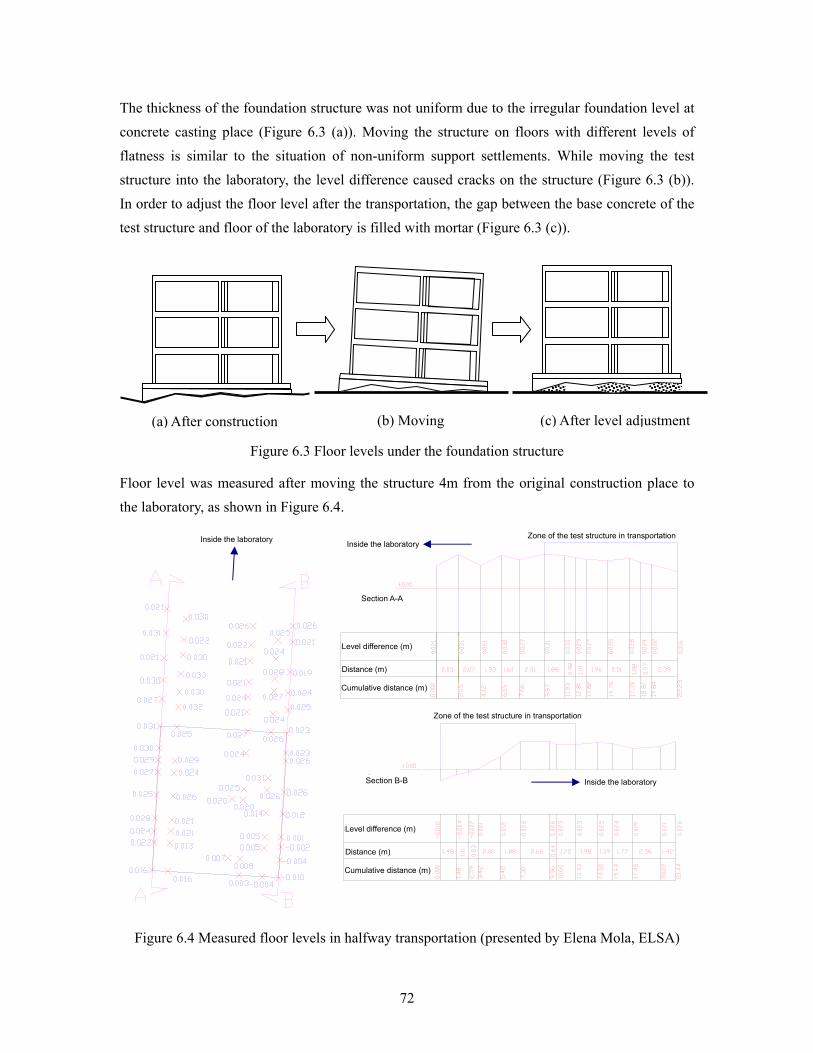
72

The thickness of the foundation structure was not uniform due to the irregular foundation level at concrete casting place (Figure 6.3 (a)). Moving the structure on floors with different levels of flatness is similar to the situation of non-uniform support settlements. While moving the test structure into the laboratory, the level difference caused cracks on the structure (Figure 6.3 (b)). In order to adjust the floor level after the transportation, the gap between the base concrete of the test structure and floor of the laboratory is filled with mortar (Figure 6.3 (c)).

Figure 6.3 Floor levels under the foundation structure

Floor level was measured after moving the structure 4m from the original construction place to the laboratory, as shown in Figure 6.4.

Figure 6.4 Measured floor levels in halfway transportation (presented by Elena Mola, ELSA)

(a) After construction (b) Moving (c) After level adjustment

Level difference (m)

Distance (m)

Cumulative distance (m)

Zone of the test structure in transportation

Section B-B Inside the laboratory

Level difference (m)

Distance (m)

Cumulative distance (m)

Zone of the test structure in transportation

Section A-A

Inside the laboratory Inside the laboratory

73

6.1.2 Investigation of cracks Locations of cracks are marked on the 1st story and 2nd story plan in Figure 6.5. Distribution of observed cracks of the 3rd story is very close to that of the 2nd story. While cracks were observed at various locations, their width was very small. Detailed descriptions of cracks on columns and beams are represented in Appendix G. Measured crack widths of the 1st story columns and the 2nd story columns are presented in Figure G1 and G3, respectively. Columns at the 1st story experienced more damage than beams and columns at other stories. Shear cracks were also observed at beams but their width was negligibly small.

N

S

E W

y

x

B12

B1 B2

B3 B4

B5 B6

B10 B8

B9 B7 B11

C1 C2 C5

C3 C4 C9

C6 C7 C8

Crack on beam

Crack on column

(a) 1st story

N

S

E W

y

x

B12

B1 B2

B3 B4

B5 B6

B10 B8

B9 B7 B11

C1 C2 C5

C3 C4 C9

C6 C7 C8

(b) 2nd story

Figure 6.5 Locations of cracks

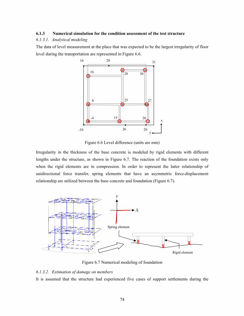
74

6.1.3 Numerical simulation for the condition assessment of the test structure 6.1.3.1. Analytical modeling The data of level measurement at the place that was expected to be the largest irregularity of floor level during the transportation are represented in Figure 6.6.

16 28 31

-10 26 26

-4

0

16 28 30

25 27

15 26x

y

Figure 6.6 Level difference (units are mm)

Irregularity in the thickness of the base concrete is modeled by rigid elements with different lengths under the structure, as shown in Figure 6.7. The reaction of the foundation exists only when the rigid elements are in compression. In order to represent the latter relationship of unidirectional force transfer, spring elements that have an asymmetric force-displacement relationship are utilized between the base concrete and foundation (Figure 6.7).

Figure 6.7 Numerical modeling of foundation

6.1.3.2. Estimation of damage on members It is assumed that the structure had experienced five cases of support settlements during the

F

∆

Rigid element

Spring element

75

transportation, as shown in Figure 6.8. The latter five cases are individually modeled and referred to as Case (A), Case (B), Case (C), Case (D) and Case (E), respectively.

Figure 6.8 Scenarios of irregular foundation

According to the investigation of cracks on the test structure in Sec. 6.1.2, the 1st story columns experienced significantly more damage than other members. In order to estimate damage on members, maximum curvature demands of damaged 1st story columns (C1, C2, C5, C6, C7 and C8) are obtained from numerical simulations for the five cases described in Figure 6.8, using nonlinear finite element analysis program ZeusNL. Table 6.1 represents the calculated maximum curvature demands.

Table 6.1 Maximum curvature demand (unit: E-6 rad./mm)

Foundation C1 C2 C5 C6 C7 C8

Case (A) 4.18 1.84 3.23 0.21 5.33 0.77

Case (B) 7.25 8.66 7.53 1.59 2.54 3.10

Case (C) 7.89 8.87 7.23 2.27 3.75 3.82

Case (D) 9.87 8.45 10.02 2.21 5.23 3.47

Case (E) 2.31 0.91 1.43 0.58 1.07 0.32

Maximum 9.87 8.87 10.02 2.27 5.33 3.82

(d) C3, C4 & C9 are not supported (e) Only C3 is not supported - Case (D) - Case (E)

(a) Uniformly supported (b) C1, C2 & C5 are not supported (c) C6, C7 & C8 are not supported - Case (A) - Case (B) - Case (C)

76

Figure 6.9 shows comparisons between the maximum curvature demands in Table 6.1 and member capacities. If the yield point is assumed to be the deformation where the strength reaches at 75% of its peak value, the maximum rotation demand is less than the yield point for each member. Considering that the simulation was performed based on the worst scenario where the most critical members and the maximum curvature demand of all cases, it was concluded that the effect of transportation on member capacities was not significant.

0

20

40

60

80

100

0 20 40 60 80 100Curvature (E-6 rad./mm)

Mom

ent (

kN-m

)

Max. curvature demandMember capacity

0

20

40

60

80

100


Mom

ent (

kN-m

) Max. curvature demandMember capacity

(a) C1 (b) C2

0

20

40

60

80

100


Mom

ent (

kN-m


0

20

40

60

80

100


Mom

ent (

kN-m

)


(c) C5 (d) C6

0

20

40

60

80

100


Mom

ent (

kN-m


0

20

40

60

80

100


Mom

ent (

kN-m

)


(e) C7 (f) C8

Figure 6.9 Comparison between maximum curvature demand and capacity

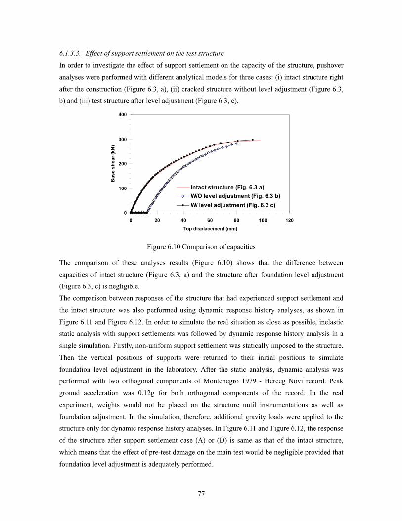
77

6.1.3.3. Effect of support settlement on the test structure In order to investigate the effect of support settlement on the capacity of the structure, pushover analyses were performed with different analytical models for three cases: (i) intact structure right after the construction (Figure 6.3, a), (ii) cracked structure without level adjustment (Figure 6.3, b) and (iii) test structure after level adjustment (Figure 6.3, c).

0

100

200

300

400

0 20 40 60 80 100 120Top displacement (mm)

Bas

e sh

ear (

kN)

Intact structure (Fig. 6.3 a)W/O level adjustment (Fig. 6.3 b)W/ level adjustment (Fig. 6.3 c)

Figure 6.10 Comparison of capacities

The comparison of these analyses results (Figure 6.10) shows that the difference between capacities of intact structure (Figure 6.3, a) and the structure after foundation level adjustment (Figure 6.3, c) is negligible. The comparison between responses of the structure that had experienced support settlement and the intact structure was also performed using dynamic response history analyses, as shown in Figure 6.11 and Figure 6.12. In order to simulate the real situation as close as possible, inelastic static analysis with support settlements was followed by dynamic response history analysis in a single simulation. Firstly, non-uniform support settlement was statically imposed to the structure. Then the vertical positions of supports were returned to their initial positions to simulate foundation level adjustment in the laboratory. After the static analysis, dynamic analysis was performed with two orthogonal components of Montenegro 1979 - Herceg Novi record. Peak ground acceleration was 0.12g for both orthogonal components of the record. In the real experiment, weights would not be placed on the structure until instrumentations as well as foundation adjustment. In the simulation, therefore, additional gravity loads were applied to the structure only for dynamic response history analyses. In Figure 6.11 and Figure 6.12, the response of the structure after support settlement case (A) or (D) is same as that of the intact structure, which means that the effect of pre-test damage on the main test would be negligible provided that foundation level adjustment is adequately performed.

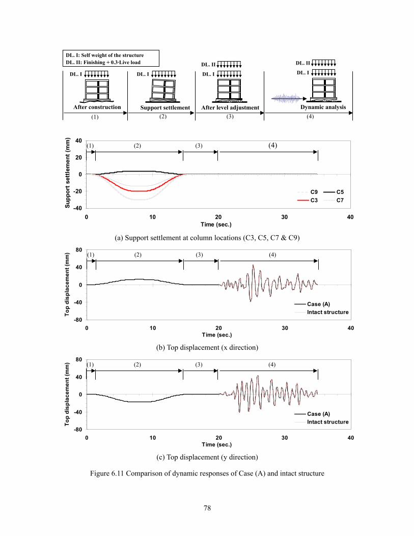
78

(a) Support settlement at column locations (C3, C5, C7 & C9)

(b) Top displacement (x direction)

(c) Top displacement (y direction)

Figure 6.11 Comparison of dynamic responses of Case (A) and intact structure

(1)

DL. I

DL. II

After level adjustment

DL. I

DL. II

Dynamic analysis

DL. I

Support settlement After construction

DL. I: Self weight of the structure DL. II: Finishing + 0.3·Live load

DL. I

(2) (3) (4)

-80

-40

0

40

80

0 10 20 30 40Time (sec.)

Top

disp

lace

men

t (m

m)

Case (A)Intact structure

(1) (2) (3) (4)

-80

-40

0

40

80

0 10 20 30 40Time (sec.)

Top

disp

lace

men

t (m

m)

Case (A)Intact structure

(1) (2) (3) (4)

-40

-20

0

20

40

0 10 20 30 40Time (sec.)

Supp

ort s

ettle

men

t (m

m)

C9 C5C3 C7

(1) (2) (3) (4)

79

(a) Support settlement at column locations (C3, C4 & C9)

(b) Top displacement (x direction)

(c) Top displacement (y direction)

Figure 6.12 Comparison of dynamic responses of Case (D) and intact structure

(1)

DL. I

DL. II

After level adjustment

DL. I

DL. II

Dynamic analysis

DL. I

Support settlement After construction

DL. I: Self weight of the structure DL. II: Finishing + 0.3·Live load

DL. I

(2) (3) (4)

-40

-20

0

20

40

0 10 20 30 40Time (sec.)

Supp

ort s

ettle

men

t (m

m)

C3C4C9

(1) (2) (3) (4)

-80

-40

0

40

80

0 10 20 30 40Time (sec.)

Top

disp

lace

men

t (m

m)

Case (D)Intact structure

D

(1) (2) (3) (4)

-80

-40

0

40

80

0 10 20 30 40Time (sec.)

Top

disp

lace

men

t (m

m)

Case (D)Intact structure

(1) (2) (3) (4)

80

6.2. DETERMINATION OF ACTUATOR MOVEMENT

Actuator movements were expected by numerical simulations to check if the limitations of loading pistons would be enough for the testing. Figure 6.13 shows expected positions of actuators and the movement of each actuator is defined by stroke (dL) and rotation angle (θ). To calculate the movements (dL and θ) of actuators, information on the location and length of each actuator were obtained from ELSA.

Figure 6.13 Description of actuators

In Section 5.4, the pre-test analytical model (Model #1) without rigid links and shear deformation at beam-column connections showed the largest top displacement. Therefore, the latter pre-test model was utilized in order to make an upper-bound estimation of the actuator movement. And for the case of unexpected change of test conditions 0.2g PGA intensity of Montenegro 1979 (Herceg Novi) is utilized for the estimation, while the suggested PGA for the test was 0.12g in Section 4.1.4. The simulation result in Figure 6.14 (a) shows that the maximum stroke demand is less than 150 mm. According to the information on actuators from ELSA, the maximum stroke capacities of actuators are ± 250 mm for the 1st level actuators and ± 500 mm for the 2nd and 3rd level actuators. And the connecting hinge at the end of each actuator can freely rotate without any angular limitation. Therefore, the capacities of actuators in ELSA are enough to perform the

Reaction wall

L

dL

L'

θ

R1

R2

R3

R4

x

Reaction wall

Reaction wall

y

(a) Position and direction of actuators (b) Relative movement of an individual actuator

81

pseudo-dynamic test of the SPEAR RC frame. The clearance during the test can be calculated by subtracting the radius (or half the sectional dimension) of the actuator from the minimum distance between the center line of actuator and corner of the test structure in Figure 6.14 (c). Since the radius of actuator in ELSA is less than 150 mm and minimum value in Figure 6.14 (c) is 280 mm, the clearance between actuators and the structure would be more than 130 mm during the test.

-150

-100

-50

0

50

100

150

200

0 3 6 9 12 15Time (sec.)

Stro

ke (m

m)

R1_1 R1_2 R1_3 R2_1 R2_2 R2_3R3_1 R3_2 R3_3 R4_1 R4_2 R4_3

(a) Stroke time histories of actuators

-2

-1

0

1

2

0 3 6 9 12 15Time (sec.)

Rot

atio

n an

gle

(deg

ree)

R1_1 R1_2 R1_3 R2_1 R2_2 R2_3R3_1 R3_2 R3_3 R4_1 R4_2 R4_3

(b) Rotation angle at the hinge of actuators

0

100

200

300

400

500

0 3 6 9 12 15Time (sec.)

Dis

tanc

e fr

om a

ctua

tor

cent

erlin

eto

cor

ners

of t

he s

truc

ture

(mm

)

R1_1 R1_2 R1_3 R2_1 R2_2 R2_3R3_1 R3_2 R3_3 R4_1 R4_2 R4_3

(c) Distance between the center line of actuators and the corner of the test structure

Figure 6.14 Estimation of actuator movement

82

6.3. GRAVITY LOAD DISTRIBUTION FOR THE TEST

Water tanks were utilized to apply the design gravity loads to the test structure. The distribution of water tanks is determined to give the same axial force on columns as the uniform load distribution, by locating the center of weight of water tanks at the center of weight of slabs. The locations and weight of water tanks on each slab are described in Figure 6.15 and Table 6.2.

Figure 6.15 Water tank distribution

Table 6.2 Weight and number of water tanks on each slab

Slab Area (m2) Weight / slab (kN) # of water tanks Weight/water tank (kN) S1 17.58 19.34 2 9.67 S2 30.63 33.69 2 16.84 S3 10.41 11.45 1 11.45 S4 16.02 17.62 2 8.81 S5 27.64 30.40 2 15.20

1.50 m

5.50 m

0.85 m

3.35 m

2.50 m

2.75 m 3.00 m

2.00 m

C8

C9

C5 C1 C2

C3 C4

C6 C7

9.67 kN

9.67 kN

8.81 kN

8.81 kN

16.84 kN 16.84 kN 11.45 kN

15.20 kN 15.20 kN

S1 S2 S3

S4

S5

x

y

83

0

100

200

300

400

500

1 2 3 4 5 6 7 8 9Column ID.

Axi

al fo

rce

(kN

)

Water tankDistributed weight

Figure 6.16 Comparison of axial forces on the 1st story columns between water tank gravity load and uniformly distributed gravity load

An analytical model with point loadings at locations of the water tanks as shown in Figure 6.15 and the other with distributed loadings as shown in Figure 2.6 were compared in the axial forces on columns. Figure 6.16 shows that the difference in column axial forces between two loading conditions is negligible. Therefore, it can be concluded that the water tank distribution is appropriately determined for the test.

84

7. EXPERIMENTAL RESULTS AND COMPARISONS

7.1. OVERVIEW OF THE FULL-SCALE PSEUDO-DYNAMIC TEST

Pseudo-dynamic (PsD) testing is an efficient hybrid of static testing and numerical analysis, which was first devised by researchers at University of Tokyo (Takanashi et al., 1977 and 1980). The latter technique is free from the shortcomings of the following methods. In static testing, determination of target displacement to simulate dynamic response of a structure is not possible, and, in numerical analyses, modeling an accurate force-deformation relationships and hysteretic damping of a structure in a highly inelastic condition is very difficult. In PsD testing, stiffness and hysteretic damping of the structure are experimentally measured to determine dynamic response of a structure by solving equations of motion. From the view point of static testing, the target displacement is determined by numerical analyses to control the hydraulic pistons. By adopting static testing setup such as reaction walls and hydraulic actuators, the advantage of the PsD testing is its applicability to very large test specimens, even to full scale civil engineering structures. The procedure is schematically represented in Figure 7.1 and the pictures of test setup are presented in Figure 7.2. In the former figure, [ ]m and [ ]c are the mass and viscous damping matrices, [ ]ι is the influence matrix which defines the relationship between degrees of freedom of the structure and directions of ground motions and { })t(f R represents measured restoring

force vector. In PsD testing, mass and viscous damping of the test structure are analytically modeled and the restoring forces are experimentally measured. Therefore, the stiffness and hysteretic damping which are accounted for by the measured restoring forces can be accurately estimated even in the highly inelastic range. After provided with the measurement of restoring forces, the numerical algorithms in the on-line computer solve the equations of motion by numerical time integration methods. The calculation results which are displacements at the next time step are imposed to the actuator controllers. Then the test structure is loaded or unloaded by actuators until the imposed target displacements are achieved. And the restoring forces are measured again to be used as input parameters to the numerical algorithm to progress to the next step. Further discussion on this topic is beyond the scope of this report. Detailed description on the pseudo-dynamic testing is presented elsewhere (Mahin and Shing, 1985, Mahin, 1987, Elnashai et al., 1990, Negro, 1996 and Molina et al., 1999). In the numerical algorithm, the discrete parameter model of the test structure has nine degrees of freedom (DOF); for each floor, two orthogonal in-plane DOFs and one rotational DOF around the vertical axis are defined at the center of the mass. Coordinate transformation between actuators

85

and floor generalized DOFs is discussed in Molina et al. (1999).

Figure 7.1 Schematic representation of pseudo-dynamic testing

Figure 7.2 Setup for the pseudo-dynamic testing

In this test, the explicit Newmark method was used because the time step (0.01 sec.) was small, in comparison to the natural periods of the test structure in the PSD algorithm (from 0.84 sec. of the 1st mode to 0.17 sec. of the 9th mode), which was enough to get stable solutions. Therefore, the target displacement can be determined by using the equilibrium conditions at the previous time step, as shown in Figure 7.1. The explicit time integration schemes are widely used to perform PSD tests due to its simplicity of the implementation and well known error propagation characteristics. However, for structures with very short natural periods or large number of DOFs, operator splitting (OS) method or α-operator splitting (OS) method is used since they provide

[ ]{ } [ ]{ } { } [ ][ ]{ }(t)uιm(t)f(t)uc(t)um gR &&&&& −=++

Measured restoring forces

Solve the equation of motion

Displacements at next time step

{ })tt(u ∆+Imposed target displacements

Actuator controller

Actuators Displacement transducers

Reference frame

Test structureNumerical algorithm

86

much better numerical stability than explicit methods (Combescure and Pegon, 1997). Four hydraulic actuators (MOOG) with loading capacity of 0.5 MN and ±0.5m (±0.25m for the first floor) stroke were installed at each floor, which makes total number of actuators twelve. Two displacement transducers were used for the displacement measurement of each actuator to guarantee stable measurement; Heidenhein liner encoder with a resolution of 2µm was mounted at the reference frame and its probe was attached to the floor along the same direction of the actuator stroke, and Temposonic internal displacement transducer was installed in the housing of actuator assemblies. Once the target displacement at each time step was achieved, the axial force at each actuator was measured by its load cell. Through discussion among the partners, the suggested intensity of 0.12 PGA in Section 4.2 was estimated to be over conservative and it was determined to use 0.15 PGA instead. After the 0.15 PGA test, only minor damage was observed at column ends and the damage level was less than expectations. Higher damage level was necessary in order to perform a research on rehabilitations which is the continual part of the SPEAR project. Therefore, the same record with higher intensity of 0.20 PGA was applied to the test structure which had already been damaged by the previous test with 0.15 PGA record.

7.2. COMPARISON OF EXPERIMENTAL RESULTS AND PRE-TEST ANALYSIS

7.2.1 Damage description Damage pattern was identified through visual inspections after the test. The 0.15g PGA test resulted in only light damage at top ends of 2nd story columns. After the 0.20g PGA test, deep cracks which smeared the interfaces between beams and columns were detected at column ends. It was obvious that the construction joints should have had a large effect on the latter cracks. Following damage patterns are identified through the visual inspection after the test. Severe damage was observed at the second story columns rather than the first story columns, while the first story was expected to be a weak story by the pre-test analysis with rigid links at column ends. After the 0.15g PGA test, cracks were observed only at top ends of the second story columns. The comparison of cracks by two tests (0.15g and 0.20g PGA) is represented in Figure 7.3. The most severe damage was observed at the center column C3 due to the large amount of axial force on it (Figure 7.3 (b)). Severe damage was also detected at the flexible-edge columns which are farther from the center of rotation, as explained in Section 4.1.4. Top ends of columns are severely damaged, while damage at the bottom of columns is light except the bottom part of C3. Damage at the bottom part of C3 is shown in Figure 7.4 (a). Beams were intact after the tests except beam 5 which is adjacent to the strong column C6. Only

87

minor cracks were observed at beam 5, as shown in Figure 7.4 (b). The cracks were induced by concentrated loading from the actuator and the high strength and stiffness of C6 as well. Cracking started or concentrated at the end line of the column which is the construction joint instead of forming a group of smaller cracks spread over the plastic hinge zone, as shown in Figure 7.4 (c).

(a) Col. 3 after 0.15g PGA test (b) Col. 3 after 0.20g PGA test

(c) Col. 4 after 0.15g PGA test (d) Col. 4 after 0.20g PGA test

(e) Col. 7 after 0.15g PGA test (f) Col. 7 after 0.20g PGA test Figure 7.3 Evolution of damage at column ends in the 2nd story

88

(g) Col. 6 after 0.15g PGA test (h) Col. 6 after 0.20g PGA test

(i) Col. 9 after 0.15g PGA test (j) Col. 9 after 0.20g PGA test

Figure 7.3 Evolution of damage at column ends in the 2nd story (continued)

(a) Damage at base of C3 (b) Crack on beam 5 (c) Cracks on Col 6

Figure 7.4 Damage on members

7.2.2 Comparison and discussion 7.2.2.1. Response histories Responses of four pre-test analytical models described in Section 5.4 are compared with the experimental results (0.15g PGA), as shown in Figure 7.5.

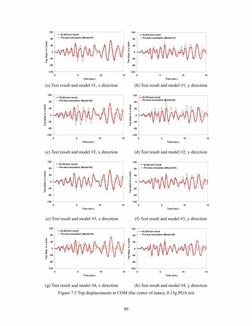
89

-120

-80

-40

0

40

80

120

0 5 10 15Time (sec.)

Top

disp

l. in

x (m

m)

ELSA test resultPre-test simulation (Model #1)

-120

-80

-40

0

40

80

120

0 5 10 15Time (sec.)

Top

disp

l. in

y (m

m)


(a) Test result and model #1, x direction (b) Test result and model #1, y direction

-120

-80

-40

0

40

80

120

0 5 10 15Time (sec.)

Top

disp

l. in

x (m

m)


-120

-80

-40

0

40

80

120

0 5 10 15Time (sec.)

Top

disp

l. in

y (m

m)


(c) Test result and model #2, x direction (d) Test result and model #2, y direction

-120

-80

-40

0

40

80

120

0 5 10 15Time (sec.)

Top

disp

l. in

x (m

m)


-120

-80

-40

0

40

80

120

0 5 10 15Time (sec.)

Top

disp

l. in

y (m

m)


(e) Test result and model #3, x direction (f) Test result and model #3, y direction

-120

-80

-40

0

40

80

120

0 5 10 15Time (sec.)

Top

disp

l. in

x (m

m)


-120

-80

-40

0

40

80

120

0 5 10 15Time (sec.)

Top

disp

l. in

y (m

m)


(g) Test result and model #4, x direction (h) Test result and model #4, y direction Figure 7.5 Top displacements at COM (the center of mass), 0.15g PGA test

90

The comparisons in Figure 7.5 are summarized in Table 7.1. The response estimations by Model #1 and Model #3 are in very good agreement with the experimental results, as shown in Figure 7.5 (a), (b), (e) and (f). Figure 7.5 (c), (d), (g) and (h) show that shorter periods than the experimental results were obtained from the response estimations by Model #2 and Model #4. The latter models adopted rigid links at column ends, as described in Table 5.7, and thus they are stiffer and stronger than the former models (Model #1 and Model # 3).

Table 7.1 Comparisons of results from pre-test analyses and the experiment

Max. top displacement Value (mm) % difference

x y x y Test result 70.06 47.52 0.00 0.00 Model #1 67.32 59.63 -3.91 25.48 Model #2 62.60 83.49 -10.65 75.70 Model #3 66.12 56.16 -5.62 18.19 Model #4 46.92 56.81 -33.04 19.56

According to the damage pattern described in Section 7.2.1, shear cracks at beam-column joints and beam hinging were not detected after the test, which means that beams were very strong and remained intact. This observation actually raises questions about the suitability of analytical models without rigid links, such as Model #1 and Model #3. Since rigid links at column ends represents a strong-beam weak-column condition, the beam-column connection behavior would have been most suitably modeled by Model #2 which has rigid links at column ends without beam-column joint shear. However, the analysis result by Model #2 is not as close to the experimental results as that of Model #1 or Model #3, as shown in Figure 7.5. This can be explained by fixed end rotation due to bond-slip in Section 7.2.2.2. Base shear time histories in Figure 7.6 and interstory drift time histories in Figure 7.7 demonstrate the accuracy of pre-test analysis by Model #1.

-400

-200

0

200

400

0 5 10 15Time (sec.)

Bas

e sh

ear i

n x

(kN

)

ELSA test resultZeusNL Simulation

-400

-200

0

200

400

0 5 10 15Time (sec.)

Bas

e sh

ear i

n y

(kN

)


(a) Base shear in x (b) Base shear in y

Figure 7.6 Comparison of base shear from experimental results and analysis by Model #1

91

-80

-40

0

40

80

0 5 10 15Time (sec.)

1st s

tory

ID. i

n x

(mm

)ELSA test resultZeusNL Simulation

-80

-40

0

40

80

0 5 10 15Time (sec.)

1st s

tory

ID. i

n y

(mm

)


(a) 1st level interstory drift in x (b) 1st level interstory drift in y

-80

-40

0

40

80

0 5 10 15Time (sec.)

2nd

stor

y ID

. in

x (m

m)


-80

-40

0

40

80

0 5 10 15Time (sec.)

2nd

stor

y ID

. in

y (m

m)


(c) 2nd level interstory drift in x (d) 2nd level interstory drift in y

-80

-40

0

40

80

0 5 10 15Time (sec.)

3rd

stor

y ID

. in

x (m

m)


-80

-40

0

40

80

0 5 10 15Time (sec.)

3rd

stor

y ID

. in

y (m

m)


(e) 3rd level interstory drift in x (f) 3rd level interstory drift in y

Figure 7.7 Comparison of interstory drift at COM (the center of mass) between experimental results and analysis by Model #1

As explained in Section 7.2.1, the response of the test structure was affected by damage at construction joints and this was not analytically modeled by the pre-test models. The latter damage became severe during the 0.20g PGA test and had more effect on the response of the test structure than it had during the 0.15g PGA test. Therefore, in the case of the 0.20g PGA test, the response estimations from pre-test analyses are not in such a good agreement as they were in the case of the 0.15g PGA test. Additional response comparisons on 0.02g PGA and 0.20g PGA test

92

are given in Appendix H. And detailed information on story level responses and bi-directional displacement of each column from experimental results of the 0.15g PGA test and the 0.20g PGA test is presented in Appendix I and Appendix J, respectively.

7.2.2.2. Bond-slip The fact that beams remained intact after the test suggests that the analytical model with rigid links (Model #2) at column ends is more appropriate than the one without rigid links (Model #1). However, the analytical model without rigid links presented closer response estimation than the one with rigid links, as represented in Section 7.2.2.1. Using rigid links in analytical simulation leads to shorter period than the experimental results. After the test, most of columns had a single clear crack at the construction joint, instead of a group of smaller cracks spread over the plastic hinge zone. This observation, and the use of smooth bars as the longitudinal reinforcement, implies that bond-slip caused the rotation at column ends and contributed to the story drift, as shown in Figure 7.8. In the pre-test simulation, bond-slip was not considered, and therefore, the analytical model with rigid links was stiffer and stronger than the test structure. Since the analytical program (ZeusNL) uses fiber elements and the plastic displacement is obtained from integrating the spread of inelasticity along the member. If the plastic hinge is defined as a center of weight of distributed curvature in plastic range, the location of plastic hinge is distant from the end of the member, as shown in Figure 7.8.

Figure 7.8 Comparison of plastic hinge locations

According to Figure 7.8, not using rigid links at column ends makes the location of plastic hinge close to the column end. Thus, the analytical model without rigid links can simulate the effect of

Model #1 Test structure Model #2

Rigid link Center line of the beam

Plastic hinge

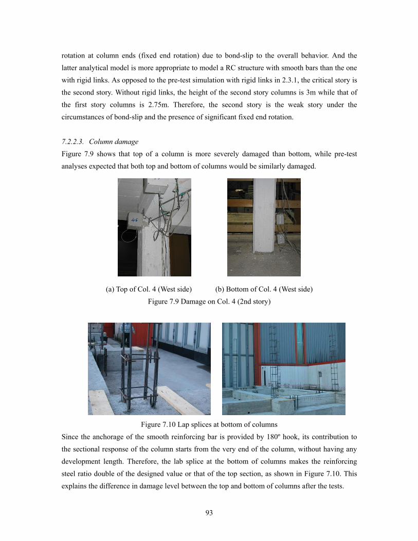
93

rotation at column ends (fixed end rotation) due to bond-slip to the overall behavior. And the latter analytical model is more appropriate to model a RC structure with smooth bars than the one with rigid links. As opposed to the pre-test simulation with rigid links in 2.3.1, the critical story is the second story. Without rigid links, the height of the second story columns is 3m while that of the first story columns is 2.75m. Therefore, the second story is the weak story under the circumstances of bond-slip and the presence of significant fixed end rotation.

7.2.2.3. Column damage Figure 7.9 shows that top of a column is more severely damaged than bottom, while pre-test analyses expected that both top and bottom of columns would be similarly damaged.

(a) Top of Col. 4 (West side) (b) Bottom of Col. 4 (West side) Figure 7.9 Damage on Col. 4 (2nd story)

Figure 7.10 Lap splices at bottom of columns

Since the anchorage of the smooth reinforcing bar is provided by 180º hook, its contribution to the sectional response of the column starts from the very end of the column, without having any development length. Therefore, the lab splice at the bottom of columns makes the reinforcing steel ratio double of the designed value or that of the top section, as shown in Figure 7.10. This explains the difference in damage level between the top and bottom of columns after the tests.

94

8. CONCLUSION

In this report, detailed description on the seismic assessment procedure of an irregular RC test building is presented. Inelastic static and dynamic analyses are performed on a 3D analytical model. Through the correlation between the analytical assessment and the full-scale test observations, a framework for improving the analytical model and furnishing the information necessary for the experiment setup is represented. The structure was designed for a full-scale pseudo-dynamic test at the Joint Research Center, Ispra, Italy under the auspices of the EU project Seismic Performance Assessment and Rehabilitation (SPEAR). Modeling considerations to accurately represent the seismic response of the test structure are presented. Inelastic behavior of RC members, torsion of irregular buildings, effect of slab diaphragm and the effect of beam-column joint shear deformation on the seismic response of the structure are accounted for. Analysis results of four different numerical models are compared, and measured data from the test as well as visually observed damage on the RC members are presented. Analytical assessment results are compared with experimental results and the appropriateness of the employed analytical assessment methods is discussed. Important conclusions are given in the pertinent part of the report. Below, the most significant issues are reiterated:

Pre-test seismic assessment of the test building

• The test building is designed to withstand only gravity loads and not in compliance with modern seismic codes. Smooth bars were utilized for the reinforcement. Members are provided with minimal amount of stirrups to withstand low levels of shear forces and the core concrete is virtually not confined. Columns are slender and more flexible than beams, and beam-column connections were built without stirrups.

• Extensive pre-test analysis was performed to investigate the effect of irregularities on the response of the test structure. Various failure criteria are defined in local and global levels and damage monitoring was performed using the results of pushover and dynamic response history analyses.

• Static pushover analyses were performed to obtain the capacity curve of the building which allows estimation of elastic and inelastic stiffness, yield displacement, ultimate displacement, peak base shear, ductility, story mechanism and qualitative estimation of the P-∆ effect.

• Dynamic response history analyses were performed for assessment objectives such as estimation of peak displacement demand, amount of torsion, member level damage and other simulation results for the test preparation.

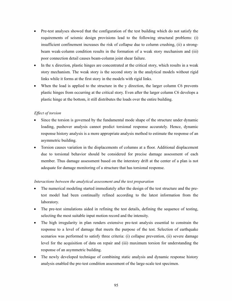
95

• Pre-test analyses showed that the configuration of the test building which do not satisfy the requirements of seismic design provisions lead to the following structural problems: (i) insufficient confinement increases the risk of collapse due to column crushing, (ii) a strong-beam weak-column condition results in the formation of a weak story mechanism and (iii) poor connection detail causes beam-column joint shear failure.

• In the x direction, plastic hinges are concentrated at the critical story, which results in a weak story mechanism. The weak story is the second story in the analytical models without rigid links while it forms at the first story in the models with rigid links.

• When the load is applied to the structure in the y direction, the larger column C6 prevents plastic hinges from occurring at the critical story. Even after the larger column C6 develops a plastic hinge at the bottom, it still distributes the loads over the entire building.

Effect of torsion

• Since the torsion is governed by the fundamental mode shape of the structure under dynamic loading, pushover analysis cannot predict torsional response accurately. Hence, dynamic response history analysis is a more appropriate analysis method to estimate the response of an asymmetric building.

• Torsion causes variation in the displacements of columns at a floor. Additional displacement due to torsional behavior should be considered for precise damage assessment of each member. Thus damage assessment based on the interstory drift at the center of a plan is not adequate for damage monitoring of a structure that has torsional response.

Interactions between the analytical assessment and the test preparation

• The numerical modeling started immediately after the design of the test structure and the pre-test model had been continually refined according to the latest information from the laboratory.

• The pre-test simulations aided in refining the test details, defining the sequence of testing, selecting the most suitable input motion record and the intensity.

• The high irregularity in plan renders extensive pre-test analysis essential to constrain the response to a level of damage that meets the purpose of the test. Selection of earthquake scenarios was performed to satisfy three criteria: (i) collapse prevention, (ii) severe damage level for the acquisition of data on repair and (iii) maximum torsion for understanding the response of an asymmetric building.

• The newly developed technique of combining static analysis and dynamic response history analysis enabled the pre-test condition assessment of the large-scale test specimen.

96

• The comparison between analytical and experimental result verifies the accuracy of the adopted analysis methods. Additionally, the successful test preparation verifies the usefulness of the pre-test analytical assessment procedure in its role of leading the test setup.

Comparison between analysis and experimental results

• Before the experiment, Model #4 in Section 5.4 which has rigid links, slab diaphragm and beam-column joint shear modeling was suggested as the most refined pre-test model.

• After the test, most damage was observed in columns, as opposed to beams, and flexible edge columns which are located far from the center of rigidity were more severely damaged than other columns, as predicted by the pre-test analyses.

• While the intact beams after the test are not in compliance with the local behavior predicted by the models without rigid links (Model #1 and Model #3), the latter models estimated the global responses very closely compared to the experimental result. This can be explained by bond-slip which was observed after the test.

• Pre-test models without rigid links (Model #1 and Model #3) provided a good estimation of reduced stiffness and strength of the test structure due to bond-slip, by forming plastic hinges closer to the column ends.

• Bond-slip prevented joint shear failure which had been expected by the pre-test analyses, because the fixed-end rotation due to the bond-slip reduced the maximum shear force transferred to the beam-column joints.

• For an RC frame with smooth bars and responding as a strong-beam weak-column system, the effect of fixed-end rotation due to bond-slip should be accounted for. Analytical modeling without bond-slip results in overestimation of the stiffness and strength.

97

9. REFERENCES

ACI 318-99, 1999, Building Code Requirements for Structural Concrete and Commentary, American Concrete Institute

Bentz, E.C., 2000, "Sectional analysis of reinforced concrete members," PhD Thesis, Department of Civil Engineering, University of Toronto, Toronto

Borzi, B., Elnashai, A.S., Facciloli, E., Calvi, G.M. and Bommer, J.J., 1998, "Inelastic spectra and ductility-damping relationships for displacement-based seismic design", ESEE Research Report No. 98-4, Imperial College, London

Borzi, B., Calvi, G.M., Elnashai, A.S., Facciloli, E. and Bommer, J.J., 2001, "Inelastic spectra for displacement-based seismic design", Soil Dynamics and Earthquake Engineering, Vol. 21(1), pp.47-61

Broderick, B.M. and Elnashai, A.S., 1994, "Seismic resistance of composite beam-columns in multi-storey structures, Part 2: Analytical model and discussion of results", Journal of Construction Steel Research, Vol. 30(3), pp. 231-258

Calvi, G.M, Magenes, G. and Pampanin, S., 2002, "Relevance of beam-column joint damage and collapse in RC frame assessment", Journal of Earthquake Engineering, Vol. 6(SI.1), pp. 75-100

Campos-Costa, A. and Pinto, A.V., 1999, "European seismic hazard scenarios - an approach to the definition of input motions for testing and reliability assessment of civil engineering structures", JRC Special publication No. X.99.XX, JRC, Ispra, Italy

CEB-FIP Model Code-1990, 1993, Design Code Comite EURO-International Du Buton, American Society of Civil Engineers

Combescure, D., and Pegon, P., 1997, "α-Operator splitting time integration technique for pseudodynamic testing error propagation analysis", Soil Dynamics and Earthquake Engineering, Vol. 16(7-8), pp.427-443

Dymiotis, C., 2000, Probabilistic seismic assessment of reinforced concrete buildings with and without masonry infills, Ph.D. Thesis, Imperial College, University of London

98

Elnashai, A.S., Elghazouli, A.Y. and Dowling, P.J., 1990, "Verification of pseudo-dynamic testing procedure for steel members", Journal of Constructional Steel Research, Vol. 16, pp. 153-161

Elnashai, A.S. and Elghazouli, A.Y., 1993, "Performance of composite steel/concrete members under earthquake loading, Part I: Analytical model", Earthquake Engineering & Structural Dynamics, Vol. 22(4), pp. 315-345

Elnashai, A.S. and Izzuddin, B.A., 1993, "Modeling of material non-linearities in steel structures subjected to transient dynamic loading", Earthquake Engineering & Structural Dynamics, Vol. 22(6), pp. 509-532

Elnashai, A.S., Papanikolaou, V. and Lee, D-H., 2002, "ZeusNL User Manual", Mid-America Earthquake Center (MAE) Report

EN 1990, 2002, Eurocode: Basis of Structural Design, European Committee for Standardization, Brussels

EN 1998-1, 2003, Final Draft of Eurocode 8: Design of Structures for Earthquake Resistance - Part 1: General rules, seismic actions and rules for buildings, European Committee for Standardization, Brussels

Fardis, M.N., 1994, Analysis and design of reinforced concrete buildings according to Eurocode 2 and 8", Configuration 3, 5 and 6, Reports on Prenormative Research in Support of Eurocode8.

Fardis, M.N., 2002, Design of an Irregular Building for the SPEAR Project - Description of the 3-Storey Structure, University of Patras

FEMA356, 2000, Prestandard and Commentary for the Seismic Rehabilitation of Buildings, Federal Emergency Management Agency, Washington, D.C.

FEMA 368 - 2000 Edition, 2001, NEHRP Recommended Provisions for Seismic Regulations for New Buildings and Other Structures, Building Seismic Safety Council, Washington, D.C.

Franchin, P., Schotanus, M. and Pinto, P., 2003, Seismic Assessment of The RC Full-Scale Test Structure to be Tested at ELSA-JCR Ispra, Pre-Test and Pre-Construction Report, University of Rome "La Sapienza", Rome

99

Hognestad, E., 1951, "A study of combined bending and axial load in reinforced concrete members", Bulletin 399, University of Illinois Engineering Experiment Station, Urbana, Illinois.

Izzuddin, B.A., Karayannis, C.G. and Elnashai, A.S., 1994, “Advanced nonlinear formulation for reinforced concrete beam-columns”, ASCE Journal of Structural Engineering, Vol. 120(10), pp. 2913-2934

Izzuddin, B.A. and Elnashai, A.S., 1989, "ADAPTIC - a program for adaptive large displacement elastoplastic dynamic analysis of steel, concrete and composite frames", Research Report ESEE Report No. 89/7, Imperial College, London

Jeong, S-H. and Elnashai, A.S., 2004, "Analytical and experimental seismic assessment of irregular RC buildings", The 13th World Conference on Earthquake Engineering, Vancouver, B.C., Canada, Paper No. 113

Kappos, A.J., 1997, "A comparative assessment of R/C structures designed to the 1995 Eurocode 8 and the 1985 CEB seismic code", The Structural Design of Tall Buildings, Vol. 6(1), pp. 59-83

MacGregor, J.G, 1997, Reinforced Concrete Mechanics and Design, the 3rd ed. Prentice Hall, Inc., New Jersey

Mahin, S.A. and Shing, P.B., 1985, "Pseudo-dynamic method for seismic testing", ASCE Journal of Structural Engineering, Vol. 111(7), pp. 1482-1503

Mahin, S.A., 1987, Development and evaluation of the pseudo-dynamic test method. Building Structures: Proceedings of the Sessions at Structures Congress '87 Related to Buildings, ASCE, New York, pp. 100-115

Mander, J.B., Priestley, M.J.N. and Park, R., 1988, “Theoretical stress-strain model for confined concrete”, ASCE Journal of Structural Engineering, Vol. 114(8), pp. 1804-1826

Martinez-Rueda, J.E. and Elnashai, A.S., 1997, "Confined concrete model under cyclic load", Materials and Structures, Vol. 30(197), pp. 139-147.

Molina, F.J., Verzeletti, G., Magonette, G., Buchet, Ph. and Geradin, M., 1999, "Bi-directional pseudodynamic test of a full-size three-storey building", Earthquake Engineering and Structural Dynamics, Vol. 28(12), pp. 1541-1566

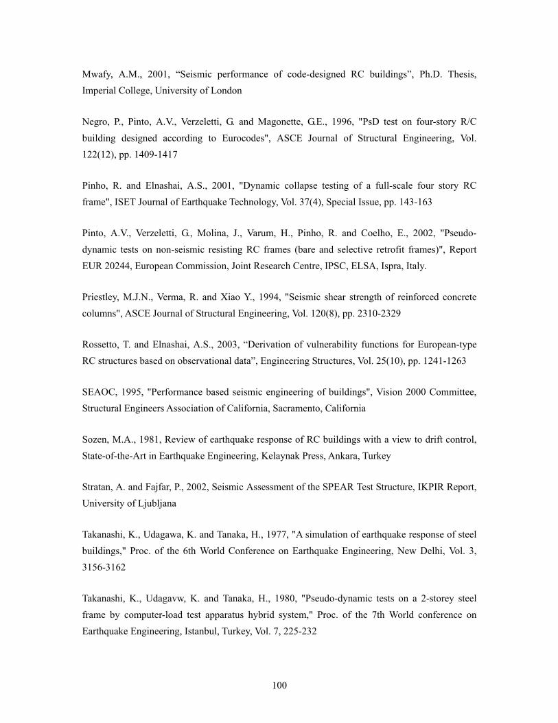
100

Mwafy, A.M., 2001, “Seismic performance of code-designed RC buildings”, Ph.D. Thesis, Imperial College, University of London

Negro, P., Pinto, A.V., Verzeletti, G. and Magonette, G.E., 1996, "PsD test on four-story R/C building designed according to Eurocodes", ASCE Journal of Structural Engineering, Vol. 122(12), pp. 1409-1417

Pinho, R. and Elnashai, A.S., 2001, "Dynamic collapse testing of a full-scale four story RC frame", ISET Journal of Earthquake Technology, Vol. 37(4), Special Issue, pp. 143-163

Pinto, A.V., Verzeletti, G., Molina, J., Varum, H., Pinho, R. and Coelho, E., 2002, "Pseudo-dynamic tests on non-seismic resisting RC frames (bare and selective retrofit frames)", Report EUR 20244, European Commission, Joint Research Centre, IPSC, ELSA, Ispra, Italy.

Priestley, M.J.N., Verma, R. and Xiao Y., 1994, "Seismic shear strength of reinforced concrete columns", ASCE Journal of Structural Engineering, Vol. 120(8), pp. 2310-2329

Rossetto, T. and Elnashai, A.S., 2003, “Derivation of vulnerability functions for European-type RC structures based on observational data”, Engineering Structures, Vol. 25(10), pp. 1241-1263

SEAOC, 1995, "Performance based seismic engineering of buildings", Vision 2000 Committee, Structural Engineers Association of California, Sacramento, California

Sozen, M.A., 1981, Review of earthquake response of RC buildings with a view to drift control, State-of-the-Art in Earthquake Engineering, Kelaynak Press, Ankara, Turkey

Stratan, A. and Fajfar, P., 2002, Seismic Assessment of the SPEAR Test Structure, IKPIR Report, University of Ljubljana

Takanashi, K., Udagawa, K. and Tanaka, H., 1977, "A simulation of earthquake response of steel buildings," Proc. of the 6th World Conference on Earthquake Engineering, New Delhi, Vol. 3, 3156-3162

Takanashi, K., Udagavw, K. and Tanaka, H., 1980, "Pseudo-dynamic tests on a 2-storey steel frame by computer-load test apparatus hybrid system," Proc. of the 7th World conference on Earthquake Engineering, Istanbul, Turkey, Vol. 7, 225-232

101

Uniform Building Code, 1997 Edition, International Conference of Building Officials, Whittier, California, 1997

Walker, S., 2001, Seismic Performance of Existing Reinforced Concrete Beam-column Joint, MS. Thesis, Department of Civil and Environmental Engineering, University of Washington, Seattle, Washington

102

Appendix A. Curvature limit states of members

Table A.1 Yield and ultimate curvatures of columns (εcu=0.0035)





1 234.22 17.50 46.00 2.63 2 154.46 16.16 64.90 4.02 C1 3 74.98 15.53 112.43 7.24 1 252.67 18.73 43.03 2.30 2 166.54 16.20 61.72 3.81 C2 3 80.13 15.59 107.91 6.92 1 407.26 21.53 33.55 1.56 2 272.34 18.76 41.67 2.22 C3 3 139.62 16.09 71.50 4.44 1 328.72 17.79 38.32 2.15 2 217.96 17.49 49.20 2.81 C4 3 107.89 15.87 86.86 5.48 1 89.56 15.68 100.19 6.39 2 57.42 15.34 133.71 8.72 C5 3 25.43 15.26 195.19 12.79 1 216.44 14.74 17.25 407.97 113.33 27.67 6.57 2 141.29 13.79 16.61 279.62 136.23 20.28 8.20 C6 3 64.29 13.43 16.02 530.49 171.24 39.49 10.69 1 150.45 16.14 67.21 4.16 2 98.51 15.77 92.33 5.85 C7 3 45.90 15.31 149.57 9.77 1 73.66 15.51 113.55 7.32 2 45.72 15.31 149.56 9.77 C8 3 18.66 14.16 211.89 14.97 1 182.26 17.40 57.59 3.31 2 121.37 15.98 79.13 4.95 C9 3 59.05 15.35 130.38 8.50

103

Table A.2 Yield and ultimate curvatures of beams (εcu=0.0035)





B4


B9


104

Table A.3 Yield and ultimate curvatures of columns (εcu=0.00456)





1 17.50 17.50 60.40 3.45 2 16.16 16.16 86.47 5.35 C1 3 15.53 15.53 148.29 9.55 1 18.73 18.73 56.55 3.02 2 16.20 16.20 81.12 5.01 C2 3 15.59 15.59 140.58 9.02 1 21.53 21.53 44.38 2.06 2 18.76 18.76 52.37 2.79 C3 3 16.09 16.09 92.83 5.77 1 17.79 17.79 48.97 2.75 2 17.49 17.49 62.80 3.59 C4 3 15.87 15.87 113.62 7.16 1 15.68 15.68 129.32 8.24 2 15.34 15.34 169.71 11.06 C5 3 15.26 15.26 231.31 15.16 1 14.74 14.74 17.25 703.38 153.20 47.71 8.88 2 13.79 13.79 16.61 375.97 182.16 27.27 10.97 C6 3 13.43 13.43 16.02 681.98 226.04 50.77* 14.11 1 16.14 16.14 87.37 5.41 2 15.77 15.77 121.36 7.69 C7 3 15.31 15.31 195.31 12.75 1 15.51 15.51 149.43 9.63 2 15.31 15.31 196.50 12.83 C8 3 14.16 14.16 263.08 18.58 1 17.40 17.40 74.56 4.28 2 15.98 15.98 103.76 6.49 C9 3 15.35 15.35 166.32 10.84

* denotes failure is induced by rupture of tension steel.

105

Table A.4 Yield and ultimate curvatures of beams (εcu=0.00456)





B4


B9


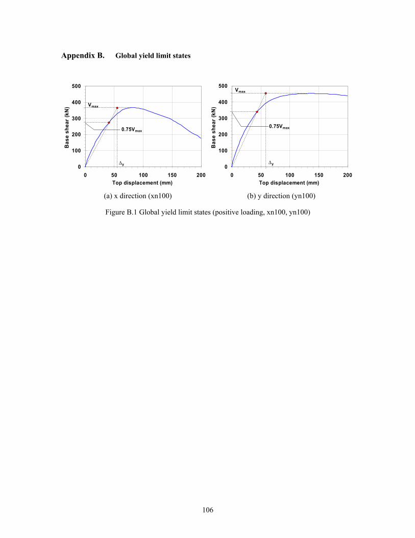
106

Appendix B. Global yield limit states

0

100

200

300

400

500


Bas

e sh

ear (

kN) Vmax

0.75Vmax

∆y 0

100

200

300

400

500


Bas

e sh

ear (

kN)

Vmax

∆y

0.75Vmax

(a) x direction (xn100) (b) y direction (yn100)

Figure B.1 Global yield limit states (positive loading, xn100, yn100)

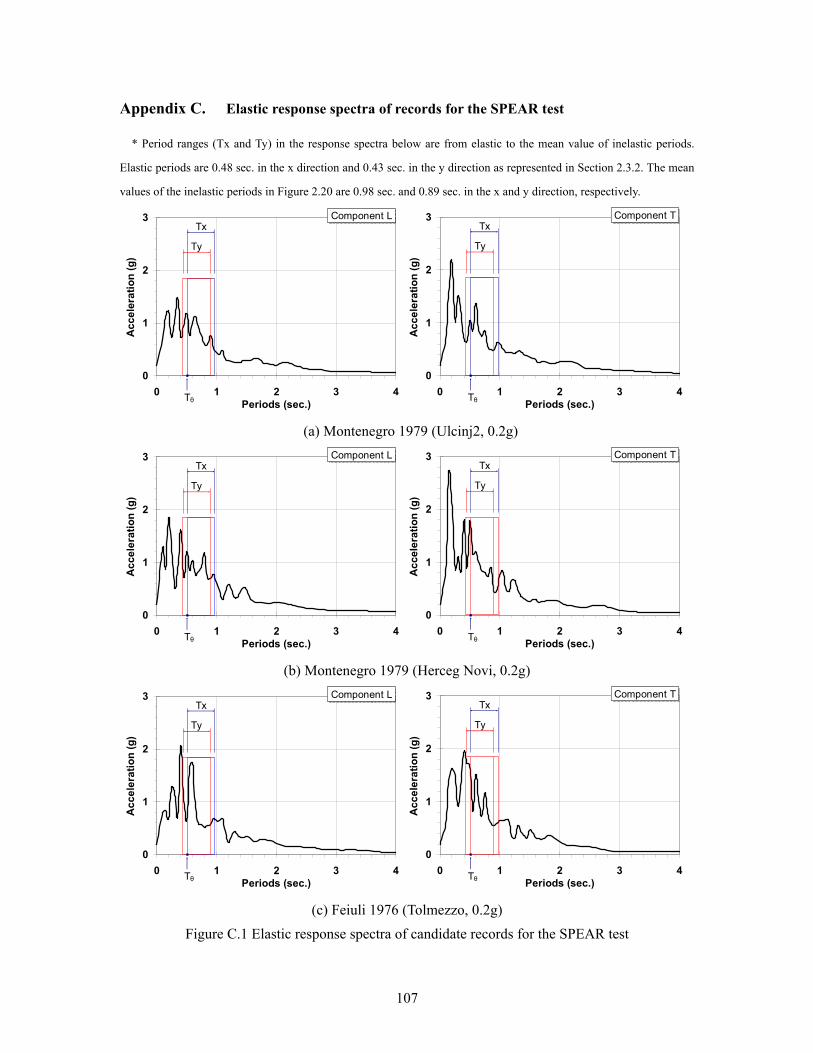
107

Appendix C. Elastic response spectra of records for the SPEAR test

* Period ranges (Tx and Ty) in the response spectra below are from elastic to the mean value of inelastic periods.

Elastic periods are 0.48 sec. in the x direction and 0.43 sec. in the y direction as represented in Section 2.3.2. The mean

values of the inelastic periods in Figure 2.20 are 0.98 sec. and 0.89 sec. in the x and y direction, respectively.

0

1

2

3


Acc

eler

atio

n (g

)

Ty

Tx

Tθ

Component L

0

1

2

3


Acc

eler

atio

n (g

)

Ty

Tx

Tθ

Component T

(a) Montenegro 1979 (Ulcinj2, 0.2g)

0

1

2

3


Acc

eler

atio

n (g

)

Ty

Tx

Tθ

Component L

0

1

2

3


Acc

eler

atio

n (g

)

Ty

Tx

Tθ

Component T

(b) Montenegro 1979 (Herceg Novi, 0.2g)

0

1

2

3


Acc

eler

atio

n (g

)

Ty

Tx

Tθ

Component L

0

1

2

3


Acc

eler

atio

n (g

)

Ty

Tx

Tθ

Component T

(c) Feiuli 1976 (Tolmezzo, 0.2g)

Figure C.1 Elastic response spectra of candidate records for the SPEAR test

108

0

1

2

3


Acc

eler

atio

n (g

)

Ty

Tx

Tθ

Component L

0

1

2

3


Acc

eler

atio

n (g

)

Ty

Tx

Tθ

Component T

(d) Imperial Valley 1940 (El Centro Array #9, 0.2g)

0

1

2

3


Acc

eler

atio

n (g

)

Ty

Tx

Tθ

Component L

0

1

2

3


Acc

eler

atio

n (g

)Ty

Tx

Tθ

Component T

(e) Kalamata 1986 (Kalamata-Prefecture, 0.2g)

0

1

2

3


Acc

eler

atio

n (g

)

Ty

Tx

Tθ

Component L

0

1

2

3


Acc

eler

atio

n (g

)

Ty

Tx

Tθ

Component T

(f) Loma Prieta 1989 (Capitola, 0.2g)

Figure C.1 Elastic response spectra of candidate records for the SPEAR test (continued)

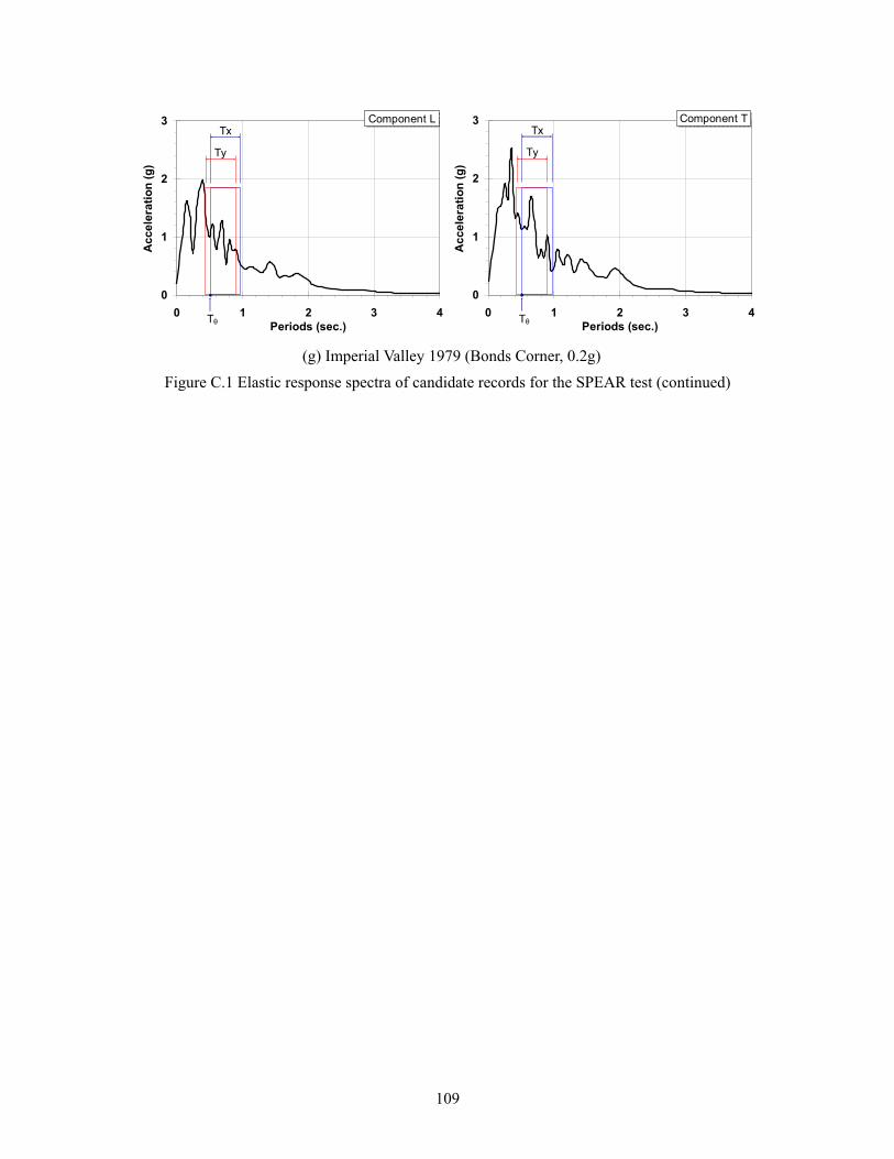
109

0

1

2

3


Acc

eler

atio

n (g

)Ty

Tx

Tθ

Component L

0

1

2

3


Acc

eler

atio

n (g

)

Ty

Tx

Tθ

Component T

(g) Imperial Valley 1979 (Bonds Corner, 0.2g)

Figure C.1 Elastic response spectra of candidate records for the SPEAR test (continued)

110

Appendix D. Angle of torsion time histories under Montenegro 1979 (Herceg Novi) with various intensities and directions

-8

-6

-4

-2

0

2

4

6

8

0 3 6 9 12 15Time (sec.)

Tors

ion

(1E-

3 ra

dian

)


-8

-6

-4

-2

0

2

4

6

8

0 3 6 9 12 15Time (sec.)

Tors

ion

(1E-

3 ra

dian

)


(a) D1 (b) D2

-8

-6

-4

-2

0

2

4

6

8

0 3 6 9 12 15Time (sec.)

Tors

ion

(1E-

3 ra

dian

)


-8

-6

-4

-2

0

2

4

6

8

0 3 6 9 12 15Time (sec.)

Tors

ion

(1E-

3 ra

dian


(c) D3 (d) D4

-8

-6

-4

-2

0

2

4

6

8

0 3 6 9 12 15Time (sec.)

Tors

ion

(1E-

3 ra

dian

)


-8

-6

-4

-2

0

2

4

6

8

0 3 6 9 12 15Time (sec.)

Tors

ion

(1E-

3 ra

dian

)


(e) D5 (f) D6

Figure D.1 Angle of torsion time histories, Montenegro 1979 - Herceg Novi, 0.12g

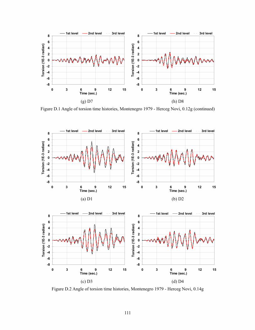
111

-8

-6

-4

-2

0

2

4

6

8

0 3 6 9 12 15Time (sec.)

Tors

ion

(1E-

3 ra

dian

)


-8

-6

-4

-2

0

2

4

6

8

0 3 6 9 12 15Time (sec.)

Tors

ion

(1E-

3 ra

dian

)


(g) D7 (h) D8

Figure D.1 Angle of torsion time histories, Montenegro 1979 - Herceg Novi, 0.12g (continued)

-8

-6

-4

-2

0

2

4

6

8

0 3 6 9 12 15Time (sec.)

Tors

ion

(1E-

3 ra

dian

)


-8

-6

-4

-2

0

2

4

6

8

0 3 6 9 12 15Time (sec.)

Tors

ion

(1E-

3 ra

dian


(a) D1 (b) D2

-8

-6

-4

-2

0

2

4

6

8

0 3 6 9 12 15Time (sec.)

Tors

ion

(1E-

3 ra

dian

)


-8

-6

-4

-2

0

2

4

6

8

0 3 6 9 12 15Time (sec.)

Tors

ion

(1E-

3 ra

dian

)


(c) D3 (d) D4


112

-8

-6

-4

-2

0

2

4

6

8

0 3 6 9 12 15Time (sec.)

Tors

ion

(1E-

3 ra

dian

)


-8

-6

-4

-2

0

2

4

6

8

0 3 6 9 12 15Time (sec.)

Tors

ion

(1E-

3 ra

dian

)


(e) D5 (f) D6

-8

-6

-4

-2

0

2

4

6

8

0 3 6 9 12 15Time (sec.)

Tors

ion

(1E-

3 ra

dian

)


-8

-6

-4

-2

0

2

4

6

8

0 3 6 9 12 15Time (sec.)

Tors

ion

(1E-

3 ra

dian

)


(g) D7 (h) D8


-8

-6

-4

-2

0

2

4

6

8

0 3 6 9 12 15Time (sec.)

Tors

ion

(1E-

3 ra

dian

)


-8

-6

-4

-2

0

2

4

6

8

0 3 6 9 12 15Time (sec.)

Tors

ion

(1E-

3 ra

dian

)


(a) D1 (b) D2


113

-8

-6

-4

-2

0

2

4

6

8

0 3 6 9 12 15Time (sec.)

Tors

ion

(1E-

3 ra

dian


-8

-6

-4

-2

0

2

4

6

8

0 3 6 9 12 15Time (sec.)

Tors

ion

(1E-

3 ra

dian

)


(c) D3 (d) D4

-8

-6

-4

-2

0

2

4

6

8

0 3 6 9 12 15Time (sec.)

Tors

ion

(1E-

3 ra

dian

)


-8

-6

-4

-2

0

2

4

6

8

0 3 6 9 12 15Time (sec.)

Tors

ion

(1E-

3 ra

dian

)


(e) D5 (f) D6

-8

-6

-4

-2

0

2

4

6

8

0 3 6 9 12 15Time (sec.)

Tors

ion

(1E-

3 ra

dian

)


-8

-6

-4

-2

0

2

4

6

8

0 3 6 9 12 15Time (sec.)

Tors

ion

(1E-

3 ra

dian

)


(g) D7 (h) D8


114

Appendix E. Interstory drift time histories under Montenegro 1979 (Herceg Novi) with various intensities and directions

-120

-90

-60

-30

0

30

60

90

120

0 3 6 9 12 15Time (sec.)

Inte

rsto

ry d

rift i

n x

(mm

)


-120

-90

-60

-30

0

30

60

90

120

0 3 6 9 12 15Time (sec.)

Inte

rsto

ry d

rift i

n y

(mm

)


(a) D1, interstory drift in x (b) D1, interstory drift in y

-120

-90

-60

-30

0

30

60

90

120

0 3 6 9 12 15Time (sec.)

Inte

rsto

ry d

rift i

n x

(mm

)


-120

-90

-60

-30

0

30

60

90

120

0 3 6 9 12 15Time (sec.)

Inte

rsto

ry d

rift i

n y

(mm


(c) D2, interstory drift in x (d) D2, interstory drift in y

-120

-90

-60

-30

0

30

60

90

120

0 3 6 9 12 15Time (sec.)

Inte

rsto

ry d

rift i

n x

(mm

)


-120

-90

-60

-30

0

30

60

90

120

0 3 6 9 12 15Time (sec.)

Inte

rsto

ry d

rift i

n y

(mm

)


(e) D3, interstory drift in x (f) D3, interstory drift in y

Figure E.1 Interstory drift time histories (at C3), Montenegro 1979 - Herceg Novi, 0.12g

115

-120

-90

-60

-30

0

30

60

90

120

0 3 6 9 12 15Time (sec.)

Inte

rsto

ry d

rift i

n x

(mm


-120

-90

-60

-30

0

30

60

90

120

0 3 6 9 12 15Time (sec.)

Inte

rsto

ry d

rift i

n y

(mm

)


(g) D4, interstory drift in x (h) D4, interstory drift in y

-120

-90

-60

-30

0

30

60

90

120

0 3 6 9 12 15Time (sec.)

Inte

rsto

ry d

rift i

n x

(mm

)


-120

-90

-60

-30

0

30

60

90

120

0 3 6 9 12 15Time (sec.)

Inte

rsto

ry d

rift i

n y

(mm

)


(i) D5, interstory drift in x (j) D5, interstory drift in y

-120

-90

-60

-30

0

30

60

90

120

0 3 6 9 12 15Time (sec.)

Inte

rsto

ry d

rift i

n x

(mm

)


-120

-90

-60

-30

0

30

60

90

120

0 3 6 9 12 15Time (sec.)

Inte

rsto

ry d

rift i

n y

(mm

)


(k) D6, interstory drift in x (l) D6, interstory drift in y

Figure E.1 Interstory drift time histories (at C3), Montenegro 1979 - Herceg Novi, 0.12g (continued)

116

-120

-90

-60

-30

0

30

60

90

120

0 3 6 9 12 15Time (sec.)

Inte

rsto

ry d

rift i

n x

(mm

)


-120

-90

-60

-30

0

30

60

90

120

0 3 6 9 12 15Time (sec.)

Inte

rsto

ry d

rift i

n y

(mm

)


(m) D7, interstory drift in x (n) D7, interstory drift in y

-120

-90

-60

-30

0

30

60

90

120

0 3 6 9 12 15Time (sec.)

Inte

rsto

ry d

rift i

n x

(mm

)


-120

-90

-60

-30

0

30

60

90

120

0 3 6 9 12 15Time (sec.)

Inte

rsto

ry d

rift i

n y

(mm

)


(o) D8, interstory drift in x (p) D8, interstory drift in y


-120

-90

-60

-30

0

30

60

90

120

0 3 6 9 12 15Time (sec.)

Inte

rsto

ry d

rift i

n x

(mm

)


-120

-90

-60

-30

0

30

60

90

120

0 3 6 9 12 15Time (sec.)

Inte

rsto

ry d

rift i

n y

(mm

)




117

-120

-90

-60

-30

0

30

60

90

120

0 3 6 9 12 15Time (sec.)

Inte

rsto

ry d

rift i

n x

(mm

)


-120

-90

-60

-30

0

30

60

90

120

0 3 6 9 12 15Time (sec.)

Inte

rsto

ry d

rift i

n y

(mm

)



-120

-90

-60

-30

0

30

60

90

120

0 3 6 9 12 15Time (sec.)

Inte

rsto

ry d

rift i

n x

(mm

)


-120

-90

-60

-30

0

30

60

90

120

0 3 6 9 12 15Time (sec.)

Inte

rsto

ry d

rift i

n y

(mm

)



-120

-90

-60

-30

0

30

60

90

120

0 3 6 9 12 15Time (sec.)

Inte

rsto

ry d

rift i

n x

(mm

)


-120

-90

-60

-30

0

30

60

90

120

0 3 6 9 12 15Time (sec.)

Inte

rsto

ry d

rift i

n y

(mm

)




118

-120

-90

-60

-30

0

30

60

90

120

0 3 6 9 12 15Time (sec.)

Inte

rsto

ry d

rift i

n x

(mm

)


-120

-90

-60

-30

0

30

60

90

120

0 3 6 9 12 15Time (sec.)

Inte

rsto

ry d

rift i

n y

(mm

)



-120

-90

-60

-30

0

30

60

90

120

0 3 6 9 12 15Time (sec.)

Inte

rsto

ry d

rift i

n x

(mm

)


-120

-90

-60

-30

0

30

60

90

120

0 3 6 9 12 15Time (sec.)

Inte

rsto

ry d

rift i

n y

(mm

)



-120

-90

-60

-30

0

30

60

90

120

0 3 6 9 12 15Time (sec.)

Inte

rsto

ry d

rift i

n x

(mm

)


-120

-90

-60

-30

0

30

60

90

120

0 3 6 9 12 15Time (sec.)

Inte

rsto

ry d

rift i

n y

(mm

)




119

-120

-90

-60

-30

0

30

60

90

120

0 3 6 9 12 15Time (sec.)

Inte

rsto

ry d

rift i

n x

(mm

)


-120

-90

-60

-30

0

30

60

90

120

0 3 6 9 12 15Time (sec.)

Inte

rsto

ry d

rift i

n y

(mm

)




-120

-90

-60

-30

0

30

60

90

120

0 3 6 9 12 15Time (sec.)

Inte

rsto

ry d

rift i

n x

(mm

)


-120

-90

-60

-30

0

30

60

90

120

0 3 6 9 12 15Time (sec.)

Inte

rsto

ry d

rift i

n y

(mm



-120

-90

-60

-30

0

30

60

90

120

0 3 6 9 12 15Time (sec.)

Inte

rsto

ry d

rift i

n x

(mm

)


-120

-90

-60

-30

0

30

60

90

120

0 3 6 9 12 15Time (sec.)

Inte

rsto

ry d

rift i

n y

(mm

)




120

-120

-90

-60

-30

0

30

60

90

120

0 3 6 9 12 15Time (sec.)

Inte

rsto

ry d

rift i

n x

(mm


-120

-90

-60

-30

0

30

60

90

120

0 3 6 9 12 15Time (sec.)

Inte

rsto

ry d

rift i

n y

(mm

)



-120

-90

-60

-30

0

30

60

90

120

0 3 6 9 12 15Time (sec.)

Inte

rsto

ry d

rift i

n x

(mm

)


-120

-90

-60

-30

0

30

60

90

120

0 3 6 9 12 15Time (sec.)

Inte

rsto

ry d

rift i

n y

(mm

)



-120

-90

-60

-30

0

30

60

90

120

0 3 6 9 12 15Time (sec.)

Inte

rsto

ry d

rift i

n x

(mm

)


-120

-90

-60

-30

0

30

60

90

120

0 3 6 9 12 15Time (sec.)

Inte

rsto

ry d

rift i

n y

(mm

)




121

-120

-90

-60

-30

0

30

60

90

120

0 3 6 9 12 15Time (sec.)

Inte

rsto

ry d

rift i

n x

(mm


-120

-90

-60

-30

0

30

60

90

120

0 3 6 9 12 15Time (sec.)

Inte

rsto

ry d

rift i

n y

(mm

)



-120

-90

-60

-30

0

30

60

90

120

0 3 6 9 12 15Time (sec.)

Inte

rsto

ry d

rift i

n x

(mm

)


-120

-90

-60

-30

0

30

60

90

120

0 3 6 9 12 15Time (sec.)

Inte

rsto

ry d

rift i

n y

(mm

)



-120

-90

-60

-30

0

30

60

90

120

0 3 6 9 12 15Time (sec.)

Inte

rsto

ry d

rift i

n x

(mm

)


-120

-90

-60

-30

0

30

60

90

120

0 3 6 9 12 15Time (sec.)

Inte

rsto

ry d

rift i

n y

(mm

)




122

Appendix F. Demand-to-capacity ratio of critical members time histories under Montenegro 1979 (Herceg Novi) with various intensities and directions

0

0.5

1

1.5

2

0 3 6 9 12 15Time (sec.)

Dem

and/

Cap

acity

(ID

)

C3 C1C2 C4

0

0.5

1

1.5

2

0 3 6 9 12 15Time (sec.)

Dem

and/

Cap

acity

(ID

)

C3 C1C2 C4

(a) D1 (b) D2

0

0.5

1

1.5

2

0 3 6 9 12 15Time (sec.)

Dem

and/

Cap

acity

(ID

)

C3 C1C2 C4

0

0.5

1

1.5

2

0 3 6 9 12 15Time (sec.)

Dem

and/

Cap

acity

(ID

)C3 C1C2 C4

(c) D3 (d) D4

0

0.5

1

1.5

2

0 3 6 9 12 15Time (sec.)

Dem

and/

Cap

acity

(ID

)

C3 C1C2 C4

0

0.5

1

1.5

2

0 3 6 9 12 15Time (sec.)

Dem

and/

Cap

acity

(ID

)

C3 C1C2 C4

(e) D5 (f) D6

Figure F.1 DCR of critical members, Montenegro 1979 - Herceg Novi, 0.12g

123

0

0.5

1

1.5

2

0 3 6 9 12 15Time (sec.)

Dem

and/

Cap

acity

(ID

)

C3 C1C2 C4

0

0.5

1

1.5

2

0 3 6 9 12 15Time (sec.)

Dem

and/

Cap

acity

(ID

)

C3 C1C2 C4

(g) D7 (h) D8

Figure F.1 DCR of critical members, Montenegro 1979 - Herceg Novi, 0.12g (continued)

0

0.5

1

1.5

2

0 3 6 9 12 15Time (sec.)

Dem

and/

Cap

acity

(ID

)

C3 C1C2 C4

0

0.5

1

1.5

2

0 3 6 9 12 15Time (sec.)

Dem

and/

Cap

acity

(ID

)

C3 C1C2 C4

(a) D1 (b) D2

0

0.5

1

1.5

2

0 3 6 9 12 15Time (sec.)

Dem

and/

Cap

acity

(ID

)

C3 C1C2 C4

0

0.5

1

1.5

2

0 3 6 9 12 15Time (sec.)

Dem

and/

Cap

acity

(ID

)

C3 C1C2 C4

(c) D3 (d) D4


124

0

0.5

1

1.5

2

0 3 6 9 12 15Time (sec.)

Dem

and/

Cap

acity

(ID

)C3 C1C2 C4

0

0.5

1

1.5

2

0 3 6 9 12 15Time (sec.)

Dem

and/

Cap

acity

(ID

)

C3 C1C2 C4

(e) D5 (f) D6

0

0.5

1

1.5

2

0 3 6 9 12 15Time (sec.)

Dem

and/

Cap

acity

(ID

)

C3 C1C2 C4

0

0.5

1

1.5

2

0 3 6 9 12 15Time (sec.)

Dem

and/

Cap

acity

(ID

)

C3 C1C2 C4

(g) D7 (h) D8


0

0.5

1

1.5

2

0 3 6 9 12 15Time (sec.)

Dem

and/

Cap

acity

(ID

)

C3 C1C2 C4

0

0.5

1

1.5

2

0 3 6 9 12 15Time (sec.)

Dem

and/

Cap

acity

(ID

)

C3 C1C2 C4

(a) D1 (b) D2


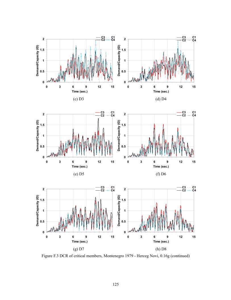
125

0

0.5

1

1.5

2

0 3 6 9 12 15Time (sec.)

Dem

and/

Cap

acity

(ID

)C3 C1C2 C4

0

0.5

1

1.5

2

0 3 6 9 12 15Time (sec.)

Dem

and/

Cap

acity

(ID

)

C3 C1C2 C4

(c) D3 (d) D4

0

0.5

1

1.5

2

0 3 6 9 12 15Time (sec.)

Dem

and/

Cap

acity

(ID

)

C3 C1C2 C4

0

0.5

1

1.5

2

0 3 6 9 12 15Time (sec.)

Dem

and/

Cap

acity

(ID

)

C3 C1C2 C4

(e) D5 (f) D6

0

0.5

1

1.5

2

0 3 6 9 12 15Time (sec.)

Dem

and/

Cap

acity

(ID

)

C3 C1C2 C4

0

0.5

1

1.5

2

0 3 6 9 12 15Time (sec.)

Dem

and/

Cap

acity

(ID

)

C3 C1C2 C4

(g) D7 (h) D8


126

Appendix G. Description of Cracks Observed from the Inspection of Pre-test Damage

Figure G.1 Cracks on the 1st story columns

S. E. N. W.

C7

0.01

S. E. N. W.

C8

0.05

0.17

0.05

S. E. N. W.

C5

S. E. N. W.

C2

0.02

S. E. N. W.

C6

0.27

0.05

S. E. N. W.

C1

0.05mm

127

Figure G.2 Cracks on the 1st story beams

y

x

B12

B1 B2

B3B4

B5B6

B10 B8

B9 B7 B11

C1 C2 C5

C3 C4C9

C6 C7C8

N. face of B1

W. face of B10

N. face of B4

E. face of B10

N

S

EW

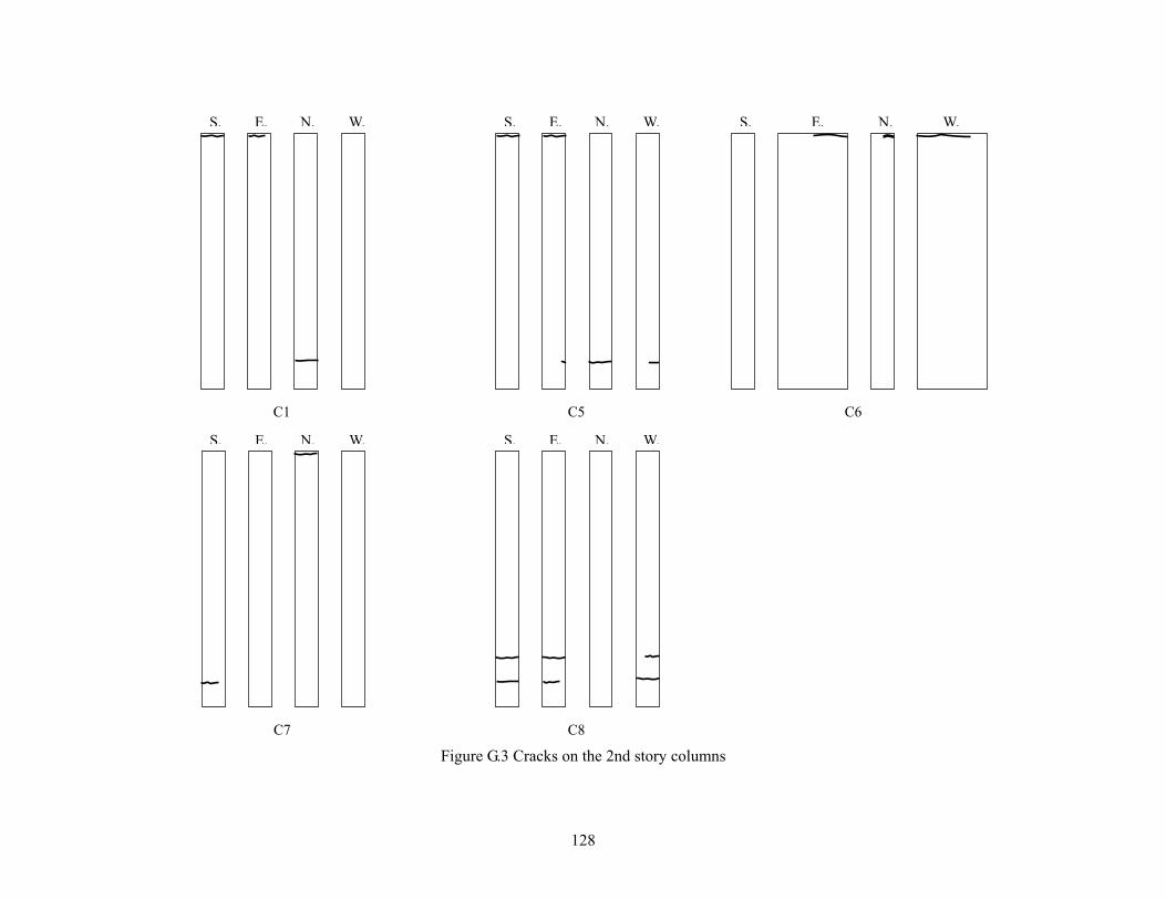
128

Figure G.3 Cracks on the 2nd story columns

S. E. N. W.

C6

S. E. N. W.

C8

S. E. N. W.

C7

S. E. N. W.

C1

S. E. N. W.

C5

129

Figure G.4 Cracks on the 2nd story beams

y

x

B12

B1 B2

B3B4

B5B6

B10 B8

B9 B7B11

C1 C2C5

C3 C4C9

C6 C7C8

W. face of B10

N. face of B4

E. face of B10

N

S

EW

S. face of B4

130

Appendix H. Comparison of the experimental results and pre-test analyses

-15

-10

-5

0

5

10

15

0 5 10 15Time (sec.)

Top

disp

l. in

x (m

m)


-15

-10

-5

0

5

10

15

0 5 10 15Time (sec.)

Top

disp

l. in

y (m

m)



-15

-10

-5

0

5

10

15

0 5 10 15Time (sec.)

Top

disp

l. in

x (m

m)


-15

-10

-5

0

5

10

15

0 5 10 15Time (sec.)

Top

disp

l. in

y (m

m)



-15

-10

-5

0

5

10

15

0 5 10 15Time (sec.)

Top

disp

l. in

x (m

m)


-15

-10

-5

0

5

10

15

0 5 10 15Time (sec.)

Top

disp

l. in

y (m

m)



-15

-10

-5

0

5

10

15

0 5 10 15Time (sec.)

Top

disp

l. in

x (m

m)


-15

-10

-5

0

5

10

15

0 5 10 15Time (sec.)

Top

disp

l. in

y (m

m)


(g) Test result and model #4, x direction (h) Test result and model #4, y direction

Figure H.1 Top displacements at the center of mass (0.02g PGA test)

131

-120

-80

-40

0

40

80

120

0 5 10 15Time (sec.)

Top

disp

l. in

x (m

m)


-120

-80

-40

0

40

80

120

0 5 10 15Time (sec.)

Top

disp

l. in

y (m

m)



-120

-80

-40

0

40

80

120

0 5 10 15Time (sec.)

Top

disp

l. in

x (m

m)


-120

-80

-40

0

40

80

120

0 5 10 15Time (sec.)

Top

disp

l. in

y (m

m)



-120

-80

-40

0

40

80

120

0 5 10 15Time (sec.)

Top

disp

l. in

x (m

m)


-120

-80

-40

0

40

80

120

0 5 10 15Time (sec.)

Top

disp

l. in

y (m

m)



-120

-80

-40

0

40

80

120

0 5 10 15Time (sec.)

Top

disp

l. in

x (m

m)


-120

-80

-40

0

40

80

120

0 5 10 15Time (sec.)

Top

disp

l. in

y (m

m)


(g) Test result and model #4, x direction (h) Test result and model #4, y direction

Figure H.2 Top displacements at the center of mass (0.20g PGA test)

132

Appendix I. Experimental results of 0.15g PGA test

-60

-30

0

30

60

0 5 10 15Time (sec.)

Inte

rsto

ry d

rift i

n x

(mm

) 1st story2nd story3rd story

-300

-200

-100

0

100

200

300

0 5 10 15Time (sec.)

Stor

y sh

ear i

n x

(kN

)


(a) Interstory drift in x direction (b) Story shear in x direction

-60

-30

0

30

60

0 5 10 15Time (sec.)

Inte

rsto

ry d

rift i

n y

(mm


-300

-200

-100

0

100

200

300

0 5 10 15Time (sec.)

Stor

y sh

ear i

n y

(kN

)


(c) Interstory drift in y direction (d) Story shear in y direction

-0.015

-0.01

-0.005

0

0.005

0.01

0.015

0 5 10 15Time (sec.)

Inte

rsto

ry to

rsio

n (r

ad.)


-1000

-500

0

500

1000

0 5 10 15Time (sec.)

Stor

y to

rque

(kN

-m)


(e) Interstory torsion (f) Story torque

Figure I. 1 Interstory drift at the center of mass and story shear (0.15g PGA)

133

-300

-200

-100

0

100

200

300

-60 -30 0 30 60Interstory drift in x (mm)

Stor

y sh

ear i

n x

(kN

)

(a) 1st story, x direction

-300

-200

-100

0

100

200

300


Stor

y sh

ear i

n x

(kN

)

(b) 2nd story, x direction

-300

-200

-100

0

100

200

300


Stor

y sh

ear i

n x

(kN

)

(c) 3rd story, x direction

-300

-200

-100

0

100

200

300


Stor

y sh

ear i

n y

(kN

)

(d) 1st story, y direction

-300

-200

-100

0

100

200

300


Stor

y sh

ear i

n y

(kN

)

(e) 2nd story, y direction

-300

-200

-100

0

100

200

300


Stor

y sh

ear i

n y

(kN

)

(f) 3rd story, y direction

-1000

-500

0

500

1000

-0.015 -0.01 -0.005 0 0.005 0.01 0.015Interstory torsion (rad.)

Stor

y to

rque

(kN

-m)

(g) 1st story, torsion

-1000

-500

0

500

1000


Stor

y to

rque

(kN

-m)

(h) 2nd story, torsion

-1000

-500

0

500

1000


Stor

y to

rque

(kN

-m)

(i) 3rd story, torsion

Figure I.2 Story force-displacement relationship (0.15g PGA)

134

-100

-50

0

50

100


Inte

rsto

ry d

rift i

n y

(mm

)C5

-100

-50

0

50

100


Inte

rsto

ry d

rift i

n y

(mm

)

C1

-100

-50

0

50

100


Inte

rsto

ry d

rift i

n y

(mm

)

C2

-100

-50

0

50

100


Inte

rsto

ry d

rift i

n y

(mm

)

C9

-100

-50

0

50

100


Inte

rsto

ry d

rift i

n y

(mm

)C3

-100

-50

0

50

100


Inte

rsto

ry d

rift i

n y

(mm

)

C4

-100

-50

0

50

100


Inte

rsto

ry d

rift i

n y

(mm

)

C8

-100

-50

0

50

100


Inte

rsto

ry d

rift i

n y

(mm

)

C6

-100

-50

0

50

100


Inte

rsto

ry d

rift i

n y

(mm

)C7

Figure I.3 Bi-directional column drift at the 1st story (0.15g PGA)

Center of rotation

y

x

C1 C2 C5

C3 C4 C9

C6 C7 C8

135

-100

-50

0

50

100


Inte

rsto

ry d

rift i

n y

(mm

)C5

-100

-50

0

50

100


Inte

rsto

ry d

rift i

n y

(mm

)

C1

-100

-50

0

50

100


Inte

rsto

ry d

rift i

n y

(mm

)

C2

-100

-50

0

50

100


Inte

rsto

ry d

rift i

n y

(mm

)

C9

-100

-50

0

50

100


Inte

rsto

ry d

rift i

n y

(mm

)C3

-100

-50

0

50

100


Inte

rsto

ry d

rift i

n y

(mm

)

C4

-100

-50

0

50

100


Inte

rsto

ry d

rift i

n y

(mm

)

C8

-100

-50

0

50

100


Inte

rsto

ry d

rift i

n y

(mm

)

C6

-100

-50

0

50

100


Inte

rsto

ry d

rift i

n y

(mm

)C7

Figure I.4 Bi-directional column drift at the 2nd story (0.15g PGA)

Center of rotation

y

x

C1 C2 C5

C3 C4 C9

C6 C7 C8

136

-100

-50

0

50

100


Inte

rsto

ry d

rift i

n y

(mm

)C5

-100

-50

0

50

100


Inte

rsto

ry d

rift i

n y

(mm

)

C1

-100

-50

0

50

100


Inte

rsto

ry d

rift i

n y

(mm

)

C2

-100

-50

0

50

100


Inte

rsto

ry d

rift i

n y

(mm

)

C9

-100

-50

0

50

100


Inte

rsto

ry d

rift i

n y

(mm

)C3

-100

-50

0

50

100


Inte

rsto

ry d

rift i

n y

(mm

)

C4

-100

-50

0

50

100


Inte

rsto

ry d

rift i

n y

(mm

)

C8

-100

-50

0

50

100


Inte

rsto

ry d

rift i

n y

(mm

)

C6

-100

-50

0

50

100


Inte

rsto

ry d

rift i

n y

(mm

)C7

Figure I.5 Bi-directional column drift at the 3rd story (0.15g PGA)

Center of rotation

y

x

C1 C2 C5

C3 C4 C9

C6 C7 C8

137

Appendix J. Experimental results of 0.20g PGA test

-60

-30

0

30

60

0 5 10 15Time (sec.)

Inte

rsto

ry d

rift i

n x

(mm


-300

-200

-100

0

100

200

300

0 5 10 15Time (sec.)

Stor

y sh

ear i

n x

(kN

)


(a) Interstory drift in x direction (b) Story shear in x direction

-60

-30

0

30

60

0 5 10 15Time (sec.)

Inte

rsto

ry d

rift i

n y

(mm


-300

-200

-100

0

100

200

300

0 5 10 15Time (sec.)

Stor

y sh

ear i

n y

(kN

)


(c) Interstory drift in y direction (d) Story shear in y direction

-0.015

-0.01

-0.005

0

0.005

0.01

0.015

0 5 10 15Time (sec.)

Inte

rsto

ry to

rsio

n (r

ad.)


-1000

-500

0

500

1000

0 5 10 15Time (sec.)

Stor

y to

rque

(kN

-m)


(e) Interstory torsion (f) Story torque

Figure J. 1 Interstory drift at the center of mass and story shear (0.20g PGA)

138

-300

-200

-100

0

100

200

300


Stor

y sh

ear i

n x

(kN

)

(a) 1st story, x direction

-300

-200

-100

0

100

200

300


Stor

y sh

ear i

n x

(kN

)

(b) 2nd story, x direction

-300

-200

-100

0

100

200

300


Stor

y sh

ear i

n x

(kN

)

(c) 3rd story, x direction

-300

-200

-100

0

100

200

300


Stor

y sh

ear i

n y

(kN

)

(d) 1st story, y direction

-300

-200

-100

0

100

200

300


Stor

y sh

ear i

n y

(kN

)

(e) 2nd story, y direction

-300

-200

-100

0

100

200

300


Stor

y sh

ear i

n y

(kN

)

(f) 3rd story, y direction

-1000

-500

0

500

1000


Stor

y to

rque

(kN

-m)

(g) 1st story, torsion

-1000

-500

0

500

1000


Stor

y to

rque

(kN

-m)

(h) 2nd story, torsion

-1000

-500

0

500

1000


Stor

y to

rque

(kN

-m)

(i) 3rd story, torsion

Figure J.2 Story force-displacement relationship (0.20g PGA)

139

-100

-50

0

50

100


Inte

rsto

ry d

rift i

n y

(mm

)C5

-100

-50

0

50

100


Inte

rsto

ry d

rift i

n y

(mm

)

C1

-100

-50

0

50

100


Inte

rsto

ry d

rift i

n y

(mm

)

C2

-100

-50

0

50

100


Inte

rsto

ry d

rift i

n y

(mm

)

C9

-100

-50

0

50

100


Inte

rsto

ry d

rift i

n y

(mm

)C3

-100

-50

0

50

100


Inte

rsto

ry d

rift i

n y

(mm

)

C4

-100

-50

0

50

100


Inte

rsto

ry d

rift i

n y

(mm

)

C8

-100

-50

0

50

100


Inte

rsto

ry d

rift i

n y

(mm

)

C6

-100

-50

0

50

100


Inte

rsto

ry d

rift i

n y

(mm

)C7

Figure J.3 Bi-directional column drift at the 1st story (0.20g PGA)

Center of rotation

y

x

C1 C2 C5

C3 C4 C9

C6 C7 C8

140

-100

-50

0

50

100


Inte

rsto

ry d

rift i

n y

(mm

)C5

-100

-50

0

50

100


Inte

rsto

ry d

rift i

n y

(mm

)

C1

-100

-50

0

50

100


Inte

rsto

ry d

rift i

n y

(mm

)

C2

-100

-50

0

50

100


Inte

rsto

ry d

rift i

n y

(mm

)

C9

-100

-50

0

50

100


Inte

rsto

ry d

rift i

n y

(mm

)C3

-100

-50

0

50

100


Inte

rsto

ry d

rift i

n y

(mm

)

C4

-100

-50

0

50

100


Inte

rsto

ry d

rift i

n y

(mm

)

C8

-100

-50

0

50

100


Inte

rsto

ry d

rift i

n y

(mm

)

C6

-100

-50

0

50

100


Inte

rsto

ry d

rift i

n y

(mm

)C7

Figure J.4 Bi-directional column drift at the 2nd story (0.20g PGA)

Center of rotation

y

x

C1 C2 C5

C3 C4 C9

C6 C7 C8

141

-100

-50

0

50

100


Inte

rsto

ry d

rift i

n y

(mm

)C5

-100

-50

0

50

100


Inte

rsto

ry d

rift i

n y

(mm

)

C1

-100

-50

0

50

100


Inte

rsto

ry d

rift i

n y

(mm

)

C2

-100

-50

0

50

100


Inte

rsto

ry d

rift i

n y

(mm

)

C9

-100

-50

0

50

100


Inte

rsto

ry d

rift i

n y

(mm

)C3

-100

-50

0

50

100


Inte

rsto

ry d

rift i

n y

(mm

)

C4

-100

-50

0

50

100


Inte

rsto

ry d

rift i

n y

(mm

)

C8

-100

-50

0

50

100


Inte

rsto

ry d

rift i

n y

(mm

)

C6

-100

-50

0

50

100


Inte

rsto

ry d

rift i

n y

(mm

)C7

Figure J.5 Bi-directional column drift at the 3rd story (0.20g PGA)

Center of rotation

y

x

C1 C2 C5

C3 C4 C9

C6 C7 C8

analytical assessment of an irregular rc full scale 3d

Documents