analytical approaches for friction induced vibration and ...analytical approaches for friction...

1

Analytical Approaches for Friction Induced Vibration and Stability Analysis

Anooshiravan FarshidianFar a, Mehrdad Noei Aghaee

a Mechanical Engineering Department, Ferdowsi University, Azadi Square, P.O. Box: 91775-

1111, Mashhad,Iran.

* [email protected]

Abstract

The traditional mass on a moving belt model without external force excitation is considered. The displacement and velocity amplitudes and the period of the friction induced vibrations can be predicted using a friction force modelled by the mean of friction characteristics. A more precise look at the non-smooth transition points of the trajectories reveals that an ex-tended friction model is looked-for. In present job, two so-called polynomial and exponential friction functions are investigated. Both of these friction laws describe a friction force that first drops off and then raises with relative interface velocity. An analytical approximation is applied in order to derive relations for the vibration amplitudes and base frequency and in parallel a stability analysis is performed. Moreover, results and phase plots are illustrated for both analytical and numerical approaches.

Keywords: Stick-Slip, Nonlinear Oscillations, Stability.

1. Introduction In order to modeling and describing friction induced vibrations, the conventional mass on a

moving belt is under investigation. We take this model for granted without discuss the validity for further applications. In driven systems friction often causes stick-slip vibrations. This non-linear effect appears in a wide range of engineering systems. Out coming sound of the violin string, brake squeal and creaking doors are of well-known stick-slip examples. For friction induced vibrations, because of unpredictable properties of contacting surfaces, there are always different valid equa-tions.

For the usual friction laws which are going to be discussed here, the kinetic friction coeffi-cient first decreases and then increases smoothly with siding speed and also there is a small but fi-nite difference between static and kinetic friction coefficients. Hence, in what will follow, the sys-tem manner in a full cycle is analyzed. For the case, a simple but handy analytical approximation, so-called perturbation approach, is utilized in order to derive approximate expressions for vibration

1st International Conference on Acoustics & Vibration (ISAV2011), Tehran, Iran, 21-22 Dec. 2011

2

amplitudes, motion period and stability conditions. In addition, the dynamical behavior of the sys-tem under self-excitation will be numerically plotted and compared with experimental data.

A wide range of researches is performed in literature. Table 1 represents a tiny summary of investigations in available data bases.

Table 1. A Compact Literature Review Author Approach Performed work

Panovko and Gubanova [1] Analytical • Introducing a polynomial expression for friction law • Self-excited oscillations occurs when the belt velocity is lower

than a critical velocity-vm

Tondl [2], Nayefeh and Mook [3] Analytical • Approximate expressions for amplitudes for the case without sticking

Ibrahim [4], McMillan [5] Analytical Numerical

• Discuss basic mechanics of friction and friction model

Popp [6] Numerical Experimental

• Presentation of models for system similar to mass on moving belt

Armstrong and Helouvy [7] Analytical • perturbation analysis for system with Stribeck friction charac-

teristics • onset of robot arm

Gao et al [8] Analytical • Expression for change in position during stick phase in system with linearized friction law

Elmer[9] Analytical • Discusses stick-slip in mass-on-belt for different friction laws • Provides expressions for stick-to-slip transition • Sketch typical local and global bifurcation scenarios

Thomsen[10] Analytical • Setup approximate expressions for stick-slip oscillations for a friction slider

Hinrichs et al [11] Numerical • Suggest an advanced extended friction model

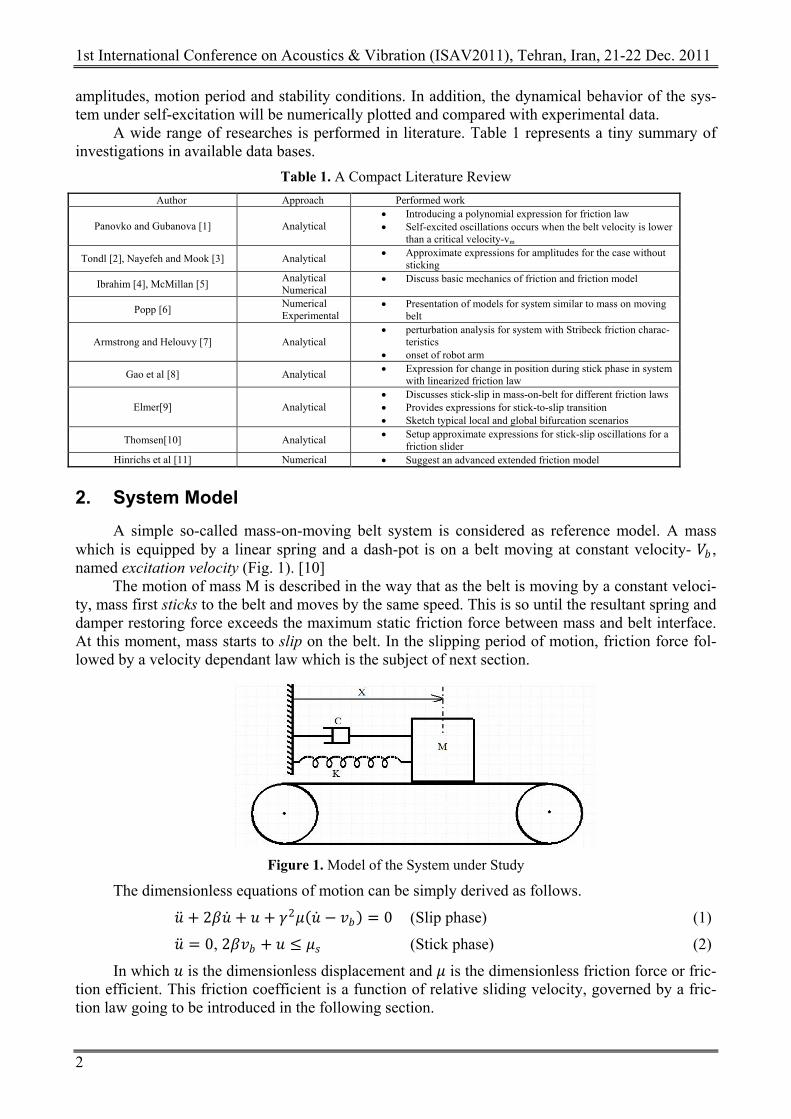
2. System Model A simple so-called mass-on-moving belt system is considered as reference model. A mass

which is equipped by a linear spring and a dash-pot is on a belt moving at constant velocity- 𝑉𝑉𝑏𝑏 , named excitation velocity (Fig. 1). [10]

The motion of mass M is described in the way that as the belt is moving by a constant veloci-ty, mass first sticks to the belt and moves by the same speed. This is so until the resultant spring and damper restoring force exceeds the maximum static friction force between mass and belt interface. At this moment, mass starts to slip on the belt. In the slipping period of motion, friction force fol-lowed by a velocity dependant law which is the subject of next section.

Figure 1. Model of the System under Study

The dimensionless equations of motion can be simply derived as follows.

�̈�𝑢 + 2𝛽𝛽�̇�𝑢 + 𝑢𝑢 + 𝛾𝛾2𝜇𝜇(�̇�𝑢 − 𝑣𝑣𝑏𝑏) = 0 (Slip phase) (1)

�̈�𝑢 = 0, 2𝛽𝛽𝑣𝑣𝑏𝑏 + 𝑢𝑢 ≤ 𝜇𝜇𝑠𝑠 (Stick phase) (2)

In which 𝑢𝑢 is the dimensionless displacement and 𝜇𝜇 is the dimensionless friction force or fric-tion efficient. This friction coefficient is a function of relative sliding velocity, governed by a fric-tion law going to be introduced in the following section.


3

3. Friction Functions The primer and of course the simplest work on dry friction is attributed to Coulomb in 1785.

Despite many years of research, the mathematical description of dry friction phenomenon is not yet fully developed. This is due to the unpredictability of microscopic characteristics of contacting sur-faces. Among a variety of approaches to this problem, the most applicable ones are introduced in following. It is pointed out that these particular forms of friction functions are not overly restricted; they resemble the friction characteristics for common use.

3.1 Consideration of Stribeck Effect; Polynomial Description The most useful and of course moderately simple friction law is the function which relates the

kinetic friction coefficient to the relative sliding velocity. This relation is the so-called Stribeck ef-fect. There are two well-known expressions which are directly regarded to this effect: polynomial expression and exponential expression.

The polynomial expression is first suggested by Panovko and Gubanova [1] and Ibrahim [4] in the terms of relative sliding velocity and also friction coefficients:

𝜇𝜇(𝑣𝑣𝑟𝑟) = 𝜇𝜇𝑠𝑠𝑠𝑠𝑠𝑠𝑠𝑠(𝑣𝑣𝑟𝑟) − 𝑘𝑘1𝑣𝑣𝑟𝑟 + 𝑘𝑘3𝑣𝑣𝑟𝑟3 (3)

Where 𝜇𝜇𝑠𝑠 is the static friction coefficient and 𝑘𝑘1 and 𝑘𝑘3 are constant introduced by 𝑘𝑘1 = 3

2(𝜇𝜇𝑠𝑠 − 𝜇𝜇𝑚𝑚)/𝑣𝑣𝑚𝑚 (4)

𝑘𝑘3 = 12

(𝜇𝜇𝑠𝑠 − 𝜇𝜇𝑚𝑚)/𝑣𝑣𝑚𝑚 3 (5)

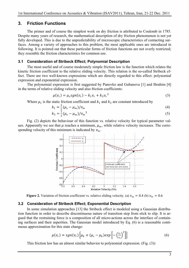
Fig. (2) depicts the behaviour of this function vs. relative velocity for typical parameter val-ues. Apparently we see that 𝜇𝜇 reaches a minimum, 𝜇𝜇𝑚𝑚 , while relative velocity increases. The corre-sponding velocity of this minimum is indicated by 𝑣𝑣𝑚𝑚 .

Figure 2. Variation of friction coefficient vs. relative sliding velocity. (a) 𝑣𝑣𝑚𝑚 = 0.4 (b) 𝑣𝑣𝑚𝑚 = 0.6

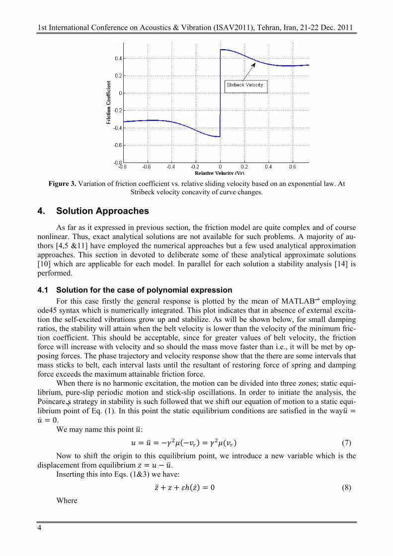
3.2 Consideration of Stribeck Effect; Exponential Description In some simulation approaches [13] the Stribeck effect is modeled using a Gaussian distribu-

tion function in order to describe discontinuous nature of transition step from stick to slip. It is ar-gued that the restraining force is a composition of all micro-actions across the interface of contain-ing surfaces and their asperities. The Gaussian model introduced by Eq. (6) is a reasonable conti-nuous approximation for this state change:

𝜇𝜇(𝑣𝑣𝑟𝑟) = 𝑠𝑠𝑠𝑠𝑠𝑠(𝑣𝑣𝑟𝑟) �𝜇𝜇𝑘𝑘 + (𝜇𝜇𝑠𝑠 − 𝜇𝜇𝑘𝑘)𝑒𝑒𝑒𝑒𝑒𝑒 �− �𝑣𝑣𝑟𝑟𝑣𝑣𝑠𝑠�

2�� (6)

This friction law has an almost similar behavior to polynomial expression. (Fig. (3))


4

Figure 3. Variation of friction coefficient vs. relative sliding velocity based on an exponential law. At

Stribeck velocity concavity of curve changes.

4. Solution Approaches As far as it expressed in previous section, the friction model are quite complex and of course

nonlinear. Thus, exact analytical solutions are not available for such problems. A majority of au-thors [4,5 &11] have employed the numerical approaches but a few used analytical approximation approaches. This section in devoted to deliberate some of these analytical approximate solutions [10] which are applicable for each model. In parallel for each solution a stability analysis [14] is performed.

4.1 Solution for the case of polynomial expression For this case firstly the general response is plotted by the mean of MATLAB® employing

ode45 syntax which is numerically integrated. This plot indicates that in absence of external excita-tion the self-excited vibrations grow up and stabilize. As will be shown below, for small damping ratios, the stability will attain when the belt velocity is lower than the velocity of the minimum fric-tion coefficient. This should be acceptable, since for greater values of belt velocity, the friction force will increase with velocity and so should the mass move faster than i.e., it will be met by op-posing forces. The phase trajectory and velocity response show that the there are some intervals that mass sticks to belt, each interval lasts until the resultant of restoring force of spring and damping force exceeds the maximum attainable friction force.

When there is no harmonic excitation, the motion can be divided into three zones; static equi-librium, pure-slip periodic motion and stick-slip oscillations. In order to initiate the analysis, the Poincare’s strategy in stability is such followed that we shift our equation of motion to a static equi-librium point of Eq. (1). In this point the static equilibrium conditions are satisfied in the way�̈�𝑢 =�̇�𝑢 = 0.

We may name this point 𝑢𝑢�:

𝑢𝑢 = 𝑢𝑢� = −𝛾𝛾2𝜇𝜇(−𝑣𝑣𝑟𝑟) = 𝛾𝛾2𝜇𝜇(𝑣𝑣𝑟𝑟) (7)

Now to shift the origin to this equilibrium point, we introduce a new variable which is the displacement from equilibrium 𝑧𝑧 = 𝑢𝑢 − 𝑢𝑢�.

Inserting this into Eqs. (1&3) we have:

�̈�𝑧 + 𝑧𝑧 + 𝜀𝜀ℎ(�̇�𝑧) = 0 (8)

Where


5

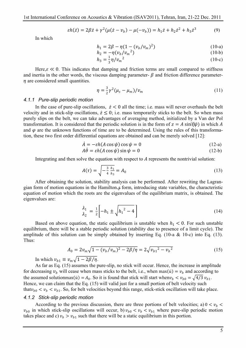
𝜀𝜀ℎ(�̇�𝑧) = 2𝛽𝛽�̇�𝑧 + 𝛾𝛾2(𝜇𝜇(�̇�𝑧 − 𝑣𝑣𝑏𝑏) − 𝜇𝜇(−𝑣𝑣𝑏𝑏)) = ℎ1�̇�𝑧 + ℎ2�̇�𝑧2 + ℎ3�̇�𝑧3 (9)

In which

ℎ1 = 2𝛽𝛽 − 𝜂𝜂(1 − (𝑣𝑣𝑏𝑏/𝑣𝑣𝑚𝑚 )2) (10-a) ℎ2 = −𝜂𝜂(𝑣𝑣𝑏𝑏/𝑣𝑣𝑚𝑚 2) (10-b) ℎ3 = 1

3𝜂𝜂/𝑣𝑣𝑚𝑚 2 (10-c)

Here,𝜀𝜀 ≪ 0. This indicates that damping and friction terms are small compared to stiffness and inertia in the other words, the viscous damping parameter- 𝛽𝛽 and friction difference parameter-𝜂𝜂 are considered small quantities.

𝜂𝜂 = 32𝛾𝛾2(𝜇𝜇𝑠𝑠 − 𝜇𝜇𝑚𝑚)/𝑣𝑣𝑚𝑚 (11)

4.1.1 Pure-slip periodic motion

In the case of pure-slip oscillations, �̇�𝑧 < 0 all the time; i.e. mass will never overhauls the belt velocity and in stick-slip oscillations, �̇�𝑧 ≤ 0; i.e. mass temporarily sticks to the belt. So when mass purely slips on the belt, we can take advantages of averaging method, initialized by a Van der Pol transformation. It is considered that the periodic solution is in the form of 𝑧𝑧 = 𝐴𝐴 sin(𝜓𝜓) in which 𝐴𝐴 and 𝜑𝜑 are the unknown functions of time are to be determined. Using the rules of this transforma-tion, these two first order differential equations are obtained and can be merely solved [12]:

�̇�𝐴 = −𝜀𝜀ℎ(𝐴𝐴 cos𝜓𝜓) cos𝜓𝜓 = 0 (12-a) 𝐴𝐴�̇�𝜃 = 𝜀𝜀ℎ(𝐴𝐴 cos𝜓𝜓) sin𝜓𝜓 = 0 (12-b)

Integrating and then solve the equation with respect to 𝐴𝐴 represents the nontrivial solution:

𝐴𝐴(𝜏𝜏) = �− 34

ℎ1ℎ3

= 𝐴𝐴0 (13)

After obtaining the solution, stability analysis can be performed. After rewriting the Lagran-gian form of motion equations in the Hamilton’s form, introducing state variables, the characteristic equation of motion which the roots are the eigenvalues of the equilibrium matrix, is obtained. The eigenvalues are:

𝜆𝜆1𝜆𝜆2

= 12�−ℎ1 ± �ℎ1

2 − 4 � (14)

Based on above equation, the static equilibrium is unstable when ℎ1 < 0. For such unstable equilibrium, there will be a stable periodic solution (stability due to presence of a limit cycle). The amplitude of this solution can be simply obtained by inserting Eq. (10-a & 10-c) into Eq. (13). Thus:

𝐴𝐴0 = 2𝑣𝑣𝑚𝑚�1 − (𝑣𝑣𝑏𝑏 𝑣𝑣𝑚𝑚⁄ )2 − 2𝛽𝛽/𝜂𝜂 = 2�𝑣𝑣𝑏𝑏12 − 𝑣𝑣𝑏𝑏2 (15)

In which 𝑣𝑣𝑏𝑏1 ≡ 𝑣𝑣𝑚𝑚�1 − 2𝛽𝛽 𝜂𝜂⁄ . As far as Eq. (15) assumes the pure-slip, no stick will occur. Hence, the increase in amplitude

for decreasing 𝑣𝑣𝑏𝑏 will cease when mass sticks to the belt, i.e., when max(�̇�𝑢) = 𝑣𝑣𝑏𝑏 and according to the assumed solutionmax(�̇�𝑢) =𝐴𝐴0. So it is found that stick will start when𝑣𝑣𝑏𝑏 < 𝑣𝑣𝑏𝑏0 = �4/3 𝑣𝑣𝑏𝑏1. Hence, we can claim that the Eq. (15) will valid just for a small portion of belt velocity such that𝑣𝑣𝑏𝑏0 < 𝑣𝑣𝑏𝑏 < 𝑣𝑣𝑏𝑏1. So, for belt velocities beyond this range, stick-stick oscillation will take place.

4.1.2 Stick-slip periodic motion

According to the previous discussion, there are three portions of belt velocities; a) 0 < 𝑣𝑣𝑏𝑏 <𝑣𝑣𝑏𝑏0 in which stick-slip oscillations will occur, b) 𝑣𝑣𝑏𝑏0 < 𝑣𝑣𝑏𝑏 < 𝑣𝑣𝑏𝑏1 where pure-slip periodic motion takes place and c) 𝑣𝑣𝑏𝑏 > 𝑣𝑣𝑏𝑏1 such that there will be a static equilibrium in this portion.


6

In the moment when𝑣𝑣𝑏𝑏 = 𝑣𝑣𝑏𝑏0, stick-slip periodic motion just started and in this moment, vi-bration amplitude will reaches to a maximum: 𝐴𝐴0 𝑚𝑚𝑚𝑚𝑒𝑒 = 𝐴𝐴0(𝑣𝑣𝑏𝑏 = 𝑣𝑣𝑏𝑏0) = 𝑣𝑣𝑏𝑏0.

In what follows, we start the analysis of stick-slip by assuming after a period of slip, mass just started to stick at time𝜏𝜏 = 𝜏𝜏0. This eventuates that �̇�𝑢(𝜏𝜏0) = 𝑣𝑣𝑏𝑏 . As long as mass sticks to the belt, it moves with a constant velocity 𝑣𝑣𝑏𝑏 , so far for sticking portion: 𝑢𝑢(𝜏𝜏) = 𝑢𝑢(𝜏𝜏0) + (𝜏𝜏 − 𝜏𝜏0)𝑣𝑣𝑏𝑏 . This equa-tion is valid until stick stops and mass starts to slip. Consequently, in stick portion, �̈�𝑢 = 0 and �̇�𝑢 = 𝑣𝑣𝑏𝑏 . So the equation of motion will get the form 𝑢𝑢 = −2𝛽𝛽𝑣𝑣𝑏𝑏 − 𝛾𝛾2𝜇𝜇(0) (see Eq. (1)). Defining time 𝜏𝜏1, in which stick ceases and mass starts slipping again on belt, represents that 𝑢𝑢(𝜏𝜏1) =−2𝛽𝛽𝑣𝑣𝑏𝑏 + 𝛾𝛾2𝜇𝜇𝑠𝑠. Here motion during slip has a fundamental difference with pure-slip periodic motion which is discussed in advanced. We can logically claim that the oscillations ensue around the equi-librium position given by Eq. (7). Hence a periodic displacement about this position can be written in the form

𝑢𝑢 = 𝐴𝐴1 𝑠𝑠𝑖𝑖𝑠𝑠 (𝜏𝜏 + 𝜑𝜑) + 𝑢𝑢� (16) �̇�𝑢 = 𝐴𝐴1 𝑐𝑐𝑐𝑐𝑠𝑠(𝜏𝜏 + 𝜑𝜑) (17)

Which in valid for the time 𝜏𝜏1 < 𝜏𝜏 < 𝜏𝜏2 where 𝜏𝜏2 is the time in which slip ends. Now in this point letting 𝜏𝜏 = 𝜏𝜏1, considering the equilibrium position in 𝜏𝜏1, then adding squares of Eqs. (16&17) to find 𝐴𝐴1, we obtain

𝐴𝐴1 = �𝑣𝑣𝑏𝑏2 + (𝛾𝛾2�𝜇𝜇𝑠𝑠 − 𝜇𝜇(𝑣𝑣𝑏𝑏)� − 2𝛽𝛽𝑣𝑣𝑏𝑏)2 = 𝑣𝑣𝑏𝑏�1 + �𝜂𝜂 �1 − 13�𝑣𝑣𝑏𝑏𝑣𝑣𝑚𝑚�

2� − 2𝛽𝛽�

2 (18)

And finally we can find the frequency of stick-slip vibrations. Based on definition of frequen-cy in the form 𝜔𝜔 = 2𝜋𝜋/𝑇𝑇, we could have 𝜔𝜔𝑠𝑠𝑠𝑠 = 2𝜋𝜋 (𝜏𝜏2 − 𝜏𝜏0)⁄ .

4.1.3 Illustrations

Despite an analytical approximation of the vibration amplitudes, numerical integration of governing ODE of system can return a better perceptive of problem. Fig. (4) which is plotted by the mean of MATLAB®, using Rung-Kutta 4th order numerical integration methods, depicts the behav-iour of system in stick-slip oscillations portion. For the case of pure-slip oscillations, after take a look at the equation of motion, we may have Fig. (4), the system response and of course the limit cycle trajectory of system which indicates the stable solution but unstable equilibrium at this condi-tion.

Figure 4. Pure-slip time response and phase plane trajectory for the values:

𝜀𝜀 = 1, 𝑣𝑣𝑚𝑚 = 0.5, 𝜇𝜇𝑠𝑠 = 0.4, 𝜇𝜇𝑚𝑚 = 0.25,𝛽𝛽 = 0.05,𝑣𝑣𝑏𝑏 = 0.4 Furthermore for the case of stick-slip oscillations, system will behaves quite differently.

This is depicted in the most proper view in Fig. (5) and finally the phase plane portrait has been illustrated for this case.


7

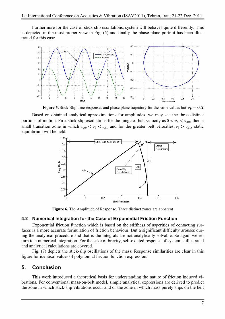
Furthermore for the case of stick-slip oscillations, system will behaves quite differently. This is depicted in the most proper view in Fig. (5) and finally the phase plane portrait has been illus-trated for this case.

Figure 5. Stick-Slip time responses and phase plane trajectory for the same values but 𝒗𝒗𝒃𝒃 = 𝟎𝟎.𝟐𝟐

Based on obtained analytical approximations for amplitudes, we may see the three distinct portions of motion. First stick-slip oscillations for the range of belt velocity as 0 < 𝑣𝑣𝑏𝑏 < 𝑣𝑣𝑏𝑏0, then a small transition zone in which 𝑣𝑣𝑏𝑏0 < 𝑣𝑣𝑏𝑏 < 𝑣𝑣𝑏𝑏1 and for the greater belt velocities, 𝑣𝑣𝑏𝑏 > 𝑣𝑣𝑏𝑏1, static equilibrium will be held.

Figure 6. The Amplitude of Response. Three distinct zones are apparent

4.2 Numerical Integration for the Case of Exponential Friction Function Exponential friction function which is based on the stiffness of asperities of contacting sur-

faces is a more accurate formulation of friction behaviour. But a significant difficulty arouses dur-ing the analytical procedure and that is the integrals are not analytically solvable. So again we re-turn to a numerical integration. For the sake of brevity, self-excited response of system is illustrated and analytical calculations are covered.

Fig. (7) depicts the stick-slip oscillations of the mass. Response similarities are clear in this figure for identical values of polynomial friction function expression.

5. Conclusion This work introduced a theoretical basis for understanding the nature of friction induced vi-

brations. For conventional mass-on-belt model, simple analytical expressions are derived to predict the zone in which stick-slip vibrations occur and or the zone in which mass purely slips on the belt


8

and beyond these portions, mass is in stable equilibrium position. Further, a more accurate friction model, exponential, is introduced which would have a more detailed description of friction behav-iour. As far as the relations mostly based on analytical approaches the can surely used in designing and laboratory experiments concerning the phenomenon under investigation.

Figure 7. Numerical Response for exponential friction law

6. REFERENCES 1. Y.G. Panovko, “ Stability and Oscillations of Elastic Systems”, Consultant Bureau, New York, 1965 2. A. Tondl, “ Quenching of Self-Excited Vibrations”, Elsevier, Amsterdam, 1991 3. A.H. Nayfeh, D.T. Mook, Nonlinear Oscillations, Wiley, New York, 1979 4. R.A. Ibrahim, “ Friction Induced Vibrations, chatter, squeal and chaos”, ASME Design Engineering

Division, DE vol.49, 1992 5. J. McMillan, “ A Nonlinear Friction Model for Self-Excited Vibrations”, Journal of Sound and Vibra-

tions 205, 323-335, 1997 6. K. Popp, “ some model problems showing stick-slip motion and chaos”, ASME Design Engineering Di-

vision, DE vol.49, 1992 7. B. Armstrong-Helouvry, P. Dupont, C. Canudas de Wit, “A survey of models, analysis tools and com-

pensation methods for the control of machines with friction”, Automatica 30 (7), 1083–1138, 1994 8. C. Gao, “ The Dynamic Analysis of Stick-Slip Motion”, Wear 173, 1994 9. F. J. Elmer, “ Nonlinear Dynamics of Dry Friction”, Journal of Physics and Math General 30, 1997 10. J. J. Thomsen, “ Using Fast Vibrations to Quench Friction Induced Oscillations”, Journal of Sound and

Vibrations 228 (5), 1079-1102, 1999 11. N. Hinrichs, M. Oestreich, K. Popp, “ On the Modeling of Friction Oscillators”, Journal of Sound and

Vibrations 216 (3), 435-459, 1997 12. J. J. Thomsen, A. Fidlin, “ Analytical Approximations for Stick-Slip Vibrations Amplitudes”, Journal of

Nonlinear Mechanics 38, 2003 13. G. J. Stein, “ On Dry Friction Modeling and Simulation in Kinematically Excited Oscillatory Systems ”,

Journal of Sound and Vibrations 311, 2008 14. J.J. Thomsen, “ Vibrations and Stability; Advanced Theory Analysis and Tools”, Springer,2003

analytical approaches for friction induced vibration and ...analytical approaches for friction...

Documents