analytical and numerical investigations of form-ﬁnding ... · such structures are called...

Analytical and numerical investigationsof form-finding methods for

tensegrity structures

Von der Fakultat Informatik, Elektrotechnik und

Informationstechnik der Universitat Stuttgart

zur Erlangung der Wurde eines

Doktors der Naturwissenschaften (Dr. rer. nat.)

genehmigte Abhandlung

Vorgelegt von

Giovani Gomez Estrada

aus Mexiko

Hauptberichter: Prof. Dr. Hans-Joachim Bungartz

Mitberichter: Prof. Dr. Manfred Bischoff

Mitberichter: Prof. Dr. Thomas Ertl

Tag der Einreichung: 19.10.2006

Tag der mundlichen Prufung: 12.07.2007

Max-Planck-Institut fur Metallforschung

und Universitat Stuttgart, 2007

Contents

1 Introduction 1

1.1 Statically indeterminate structures . . . . . . . . . . . . . . . . . . . . . . 2

1.2 Tensegrity structures . . . . . . . . . . . . . . . . . . . . . . . . . . . . . . 4

1.3 Applications and challenges of tensegrity structures . . . . . . . . . . . . . 5

1.4 State of the art of form-finding methods for tensegrity structures . . . . . . 7

1.5 Overview of the research . . . . . . . . . . . . . . . . . . . . . . . . . . . . 9

1.6 Outline of the dissertation . . . . . . . . . . . . . . . . . . . . . . . . . . . 11

2 Tensegrity structures 13

2.1 Attraction and repulsion . . . . . . . . . . . . . . . . . . . . . . . . . . . . 13

2.2 Basic hypotheses . . . . . . . . . . . . . . . . . . . . . . . . . . . . . . . . 14

2.3 Applications . . . . . . . . . . . . . . . . . . . . . . . . . . . . . . . . . . . 16

2.4 Geometry and tension coefficients . . . . . . . . . . . . . . . . . . . . . . . 18

2.5 Rank conditions and nullity . . . . . . . . . . . . . . . . . . . . . . . . . . 21

2.6 Initial stiffness . . . . . . . . . . . . . . . . . . . . . . . . . . . . . . . . . . 23

2.7 Form-finding of tensegrity structures . . . . . . . . . . . . . . . . . . . . . 25

2.8 Example: the triplex . . . . . . . . . . . . . . . . . . . . . . . . . . . . . . 29

3 Analytical form-finding of tensegrity cylinders 33

3.1 Tensegrity cylinders . . . . . . . . . . . . . . . . . . . . . . . . . . . . . . . 33

3.2 Geometric arrangement of tensegrity cylinders . . . . . . . . . . . . . . . . 34

i

3.3 Analytical form-finding procedure . . . . . . . . . . . . . . . . . . . . . . . 37

3.4 Enumerating solutions: regular convex and star polygons . . . . . . . . . . 40

3.5 Analysis of tension coefficients, forces and lengths . . . . . . . . . . . . . . 43

3.6 A full example: the 9-plex . . . . . . . . . . . . . . . . . . . . . . . . . . . 46

3.7 Implementation . . . . . . . . . . . . . . . . . . . . . . . . . . . . . . . . . 49

3.8 Conclusions and final remarks . . . . . . . . . . . . . . . . . . . . . . . . . 51

4 Stability and non-uniqueness of the solution for tensegrity cylinders 52

4.1 Introduction . . . . . . . . . . . . . . . . . . . . . . . . . . . . . . . . . . . 52

4.2 Stability and global equilibrium . . . . . . . . . . . . . . . . . . . . . . . . 53

4.3 Non-uniqueness of the analytical solution for tensegrity cylinders . . . . . . 56

4.4 Initial stiffness . . . . . . . . . . . . . . . . . . . . . . . . . . . . . . . . . . 61

4.5 A full example: the 30-plex . . . . . . . . . . . . . . . . . . . . . . . . . . 66


5 Numerical form-finding of tensegrity structures 73

5.1 Introduction . . . . . . . . . . . . . . . . . . . . . . . . . . . . . . . . . . . 73

5.2 Form-finding with prototypes . . . . . . . . . . . . . . . . . . . . . . . . . 75

5.3 From tension coefficients to coordinates . . . . . . . . . . . . . . . . . . . . 76

5.4 From coordinates to tension coefficients . . . . . . . . . . . . . . . . . . . . 79

5.5 Examples of 2D and 3D tensegrity structures . . . . . . . . . . . . . . . . . 81

5.6 Implementation . . . . . . . . . . . . . . . . . . . . . . . . . . . . . . . . . 89

5.7 Complexity and convergence . . . . . . . . . . . . . . . . . . . . . . . . . . 92

5.8 Numerical example . . . . . . . . . . . . . . . . . . . . . . . . . . . . . . . 95


6 Conclusions and final remarks 100

6.1 Analytical form-finding . . . . . . . . . . . . . . . . . . . . . . . . . . . . . 100

ii

6.2 Numerical form-finding . . . . . . . . . . . . . . . . . . . . . . . . . . . . . 101

6.3 Limitations and opportunities . . . . . . . . . . . . . . . . . . . . . . . . . 102

Bibliography 104

Summary 119

Zusammenfassung 129

Resume 138

Acknowledgements 140

Index 141

iii

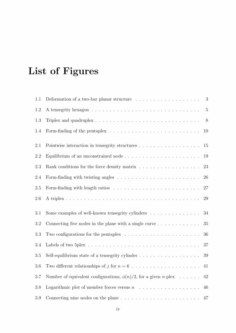
List of Figures

1.1 Deformation of a two-bar planar structure . . . . . . . . . . . . . . . . . . 3

1.2 A tensegrity hexagon . . . . . . . . . . . . . . . . . . . . . . . . . . . . . . 5

1.3 Triplex and quadruplex . . . . . . . . . . . . . . . . . . . . . . . . . . . . . 8

1.4 Form-finding of the pentaplex . . . . . . . . . . . . . . . . . . . . . . . . . 10

2.1 Pointwise interaction in tensegrity structures . . . . . . . . . . . . . . . . . 15

2.2 Equilibrium of an unconstrained node . . . . . . . . . . . . . . . . . . . . . 19

2.3 Rank conditions for the force density matrix . . . . . . . . . . . . . . . . . 23

2.4 Form-finding with twisting angles . . . . . . . . . . . . . . . . . . . . . . . 26

2.5 Form-finding with length ratios . . . . . . . . . . . . . . . . . . . . . . . . 27

2.6 A triplex . . . . . . . . . . . . . . . . . . . . . . . . . . . . . . . . . . . . . 29

3.1 Some examples of well-known tensegrity cylinders . . . . . . . . . . . . . . 34

3.2 Connecting five nodes in the plane with a single curve . . . . . . . . . . . . 35

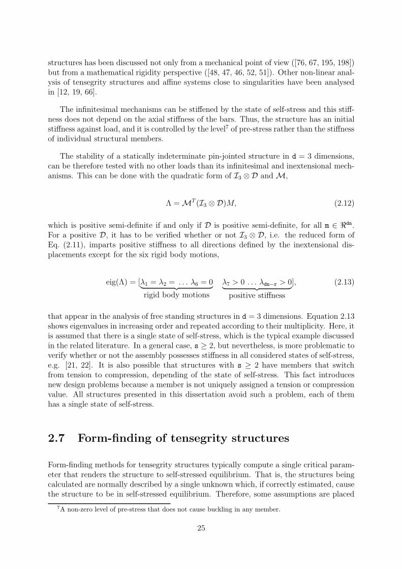
3.3 Two configurations for the pentaplex . . . . . . . . . . . . . . . . . . . . . 36

3.4 Labels of two 5plex . . . . . . . . . . . . . . . . . . . . . . . . . . . . . . . 37

3.5 Self-equilibrium state of a tensegrity cylinder . . . . . . . . . . . . . . . . . 39

3.6 Two different relationships of j for n = 6 . . . . . . . . . . . . . . . . . . . 41

3.7 Number of equivalent configurations, φ(n)/2, for a given n-plex . . . . . . 42

3.8 Logarithmic plot of member forces versus n . . . . . . . . . . . . . . . . . 46

3.9 Connecting nine nodes on the plane . . . . . . . . . . . . . . . . . . . . . . 47

iv

3.10 Three possible solutions for the 9-plex . . . . . . . . . . . . . . . . . . . . 48

3.11 Implementation of the form-finding method . . . . . . . . . . . . . . . . . 50

4.1 Elastic strain energy . . . . . . . . . . . . . . . . . . . . . . . . . . . . . . 56

4.2 Example of asymmetric tensegrity structures . . . . . . . . . . . . . . . . . 60

4.3 Extra tensile elements in a star-like cylinder . . . . . . . . . . . . . . . . . 63

4.4 Stabilisation of star-like cylinders . . . . . . . . . . . . . . . . . . . . . . . 64

4.5 Four possible solutions for a 30-plex . . . . . . . . . . . . . . . . . . . . . . 67

4.6 Influence of j to the incircle of a 30-plex . . . . . . . . . . . . . . . . . . . 70

5.1 Outline of the numerical form-finding procedure . . . . . . . . . . . . . . . 76

5.2 Pseudocode . . . . . . . . . . . . . . . . . . . . . . . . . . . . . . . . . . . 81

5.3 Examples of planar tensegrities . . . . . . . . . . . . . . . . . . . . . . . . 83

5.4 Form-finding of the expanded octahedron . . . . . . . . . . . . . . . . . . . 84

5.5 Form-finding of the truncated tetrahedron . . . . . . . . . . . . . . . . . . 85

5.6 Form-finding of the truncated icosahedron . . . . . . . . . . . . . . . . . . 87

5.7 Examples of cylindrical tensegrities of order n . . . . . . . . . . . . . . . . 88

5.8 An implementation of the form-finding method . . . . . . . . . . . . . . . . 90

5.9 Main equations of the proposed form-finding procedure . . . . . . . . . . . 91

5.10 Computing time . . . . . . . . . . . . . . . . . . . . . . . . . . . . . . . . . 93

5.11 Numerical example . . . . . . . . . . . . . . . . . . . . . . . . . . . . . . . 97

6.1 Analytical investigations of cylindrical tensegrity structures . . . . . . . . . 121

6.2 Pseudocode . . . . . . . . . . . . . . . . . . . . . . . . . . . . . . . . . . . 125

6.3 Numerical investigations of tensegrity structures . . . . . . . . . . . . . . . 126

6.4 Analytische Untersuchung . . . . . . . . . . . . . . . . . . . . . . . . . . . 131

6.5 Pseudocode . . . . . . . . . . . . . . . . . . . . . . . . . . . . . . . . . . . 134

6.6 Analytische Untersuchung . . . . . . . . . . . . . . . . . . . . . . . . . . . 136

v

List of Tables

3.1 Number of equivalent solutions for some tensegrity structures . . . . . . . . 43

3.2 Calculation of the 9-plex . . . . . . . . . . . . . . . . . . . . . . . . . . . . 50

4.1 Tension coefficients of 3-plexes found with random prototypes . . . . . . . 59

4.2 Member lengths of a 3-plex found with random prototypes . . . . . . . . . 59

4.3 Tension coefficients of one extended 5-plex with j = 2 . . . . . . . . . . . . 65

4.4 Example of tension coefficients . . . . . . . . . . . . . . . . . . . . . . . . . 68

4.5 Example of lengths . . . . . . . . . . . . . . . . . . . . . . . . . . . . . . . 68

4.6 Example of forces . . . . . . . . . . . . . . . . . . . . . . . . . . . . . . . . 68

4.7 Eigenvalues and initial stiffness . . . . . . . . . . . . . . . . . . . . . . . . 69

5.1 Iterations of the numerical form-finding procedure . . . . . . . . . . . . . . 98

vi

List of Main Symbols and Functions

Scalars

b Number of edges or members.

d Number of geometric dimensions.

m Number of mechanisms.

n Number of vertices or nodes.

r Rank of the equilibrium matrix.

s Number of states of self-stress.

Vectors

d Displacements or mechanisms.

q0 Prototypes of member forces.

t Tension coefficients or force density coefficients.

x Cartesian coordinates in the x-axis.

y Cartesian coordinates in the y-axis.

z Cartesian coordinates in the z-axis.

Matrices

A Equilibrium matrix.

C Incidence matrix.

D Force density matrix.

Kt Tangent stiffness matrix.

M Basis of mechanisms.

Q Diagonal matrix of tension coefficients.

T Basis of tension coefficients.

vii

Functions

arg min(⋆)

(⋆⋆) Argument (⋆) in which the function (⋆⋆) is minimised.

eig(⋆) Eigenvalues of (⋆).

φ(⋆) Euler’s totient function of (⋆).

GCD(⋆, ⋆⋆) Greatest common divisor of (⋆) and (⋆⋆).

⊗ Kronecker tensor product.

rank(⋆) Rank of matrix (⋆).

sgn(⋆) Sign of elements in vector (⋆).

diag(⋆) Square matrix with the vector (⋆) along its diagonal.

(⋆)T Transpose of (⋆).

‖(⋆)‖ Vector norm of (⋆).

viii

Chapter 1

Introduction

Computational mechanics (CM) uses advanced computing methods, mechanics, physics,and mathematics in the study of modern engineering systems governed by the laws ofmechanics. The scope of the research on this topic includes theoretical and computingmethods used in many fields, such as solid and structural mechanics, fluid mechanics,fracture mechanics, transport phenomena, and heat transfer. Many of the mathemat-ical models used in CM are based on fundamental laws of physics (e.g., the principlesof motion, energy, and force) developed over centuries of research on the behaviour ofmechanical systems under the action of natural forces.

CM is a fundamental part of computational science and engineering, from which ittakes its strong interdisciplinary character. Computational science and engineering, alongwith theory and experiment, is used to develop conceptual and mathematical abstractionsfor simulation of a wide range of physical and engineering systems. Hence, research withinCM emphasises a multidisciplinary approach in which mechanics and physics converge notonly through analytical and computational methods, but also through novel numericalmethods developed in their own right. The latter methods especially are of primaryinterest because general weighted residual methods, such as finite element, boundaryelement, and finite difference, can be applied to real-life problems.

CM encompasses design, analysis, and simulation of products that are used in everyfacet of modern life. It has a wide impact on automotive, aerospace, defence, chemi-cal, communication, and biomedical fields; and in virtually any manufacturing industry,including power generation. A discipline that allows advances in modern science andtechnology, CM will continue to play an important role in future industrial developmentsalso.

CM has been an integral component of scientific and industrial research for long be-cause of its various uses. A striking feature common to most current large-scale research isthe power, maturity, and sophistication reached by this branch of computational scienceand engineering. Some other areas, indeed, have conclusively demonstrated that largescale computer simulations are the only means by which key physical phenomena can beelucidated.

1

Both CM and its parent area, computational science and engineering, are by natureinter- and multi-disciplinary. Their foundations lie in mechanics, physics and mathemat-ics, and they largely depends on computing methods, but nevertheless it is analytical andnumerical modelling at their heart.

1.1 Statically indeterminate structures

One of the many fields in which CM plays an important role is in analysing complexelasticity and structural analysis problems found in the design of structures, such as hy-perbolic paraboloids, cable grids, barrel vaults, membranes, domes, towers, tensegritystructures, prestressed assemblies, foldable structures, and many other cable arrange-ments. To do so, it brings together theories of mechanics, such as elasticity theory andstrength of materials, and advanced computing algorithms to model structures of severaldegrees of freedom, large size, and complexity.

A common feature of many of those structures is that their static equilibrium equa-tions are not sufficient for uniquely determining internal and reaction forces. Hence,such structures are called statically indeterminate structures. There are important ar-eas of study in CM that deal with modelling, form-finding and displacement analysis ofstatically indeterminate structures. One statically indeterminate structure, which has at-tracted great attention recently, is the class of tensegrity structures. As found in otherstatically indeterminate structures, the geometry plays an important role for their anal-ysis. Figure 1.1 shows a simple example that illustrates this problem of statics where thestatical (in-)determinacy largely depends on the geometry and pre-stress the structure hasadopted.

For instance, the central node in Fig. 1.1a can sustain and equilibrate a vertical loadP by applying compressive axial forces to the bars. The structure is rigid up to certainlevel in which the “snap-through” phenomenon appears. It is a statically determinatestructure. On the other hand, when the bars are arranged as shown in Fig. 1.1b, with nopre-stress, the two-bar structure has no initial resistance to vertical loads. It is called a“finite” mechanism. The situation is however different if pre-stress is present, see Fig. 1.1c.Here, the pre-stress is t0 6= 0, i.e. the bars are in tension so t0 > 0, and the structure hasan initial resistance against a vertical load P . Intuitively, if the bars behave as elasticsprings, it is seen that a deflection ∆ due to P is a function of the pre-stress level t0. Inthis example, the relationship (e.g. see [117]) between the pre-stress t0, load P and smalldisplacement ∆, is:

EA

L0∆3 + 2t0L0∆− PL2

0 = 0,

where EA is the axial stiffness of both bars. Thus, when the pre-stress is not present

2

��

��

��

��

��

��

��

��

��

��

��

��

L0L0

(a)

P

P

L0L0

(b)

P

L0L0

∆

t0 t0

t + t0t + t0

(c)

Fig. 1.1: Deformation of a two-bar planar structure : (a) the length of both bars islarger than L0, here the central node is capable of sustaining a load P by introducingcompressive axial forces in the two bars, until certain level in which the “snap-through”phenomenon is observed; (b) when the length of both bars is L0 the central node is unableto resist a load P ; (c) a pre-stress level t0 > 0 appears when the initial bar lengths areshorter than L0, here the central node undergoes a displacement ∆ capable of equilibratingthe vertical load P .

(t0 = 0 as in Fig. 1.1b) the load,

P = 2∆t0L0

+EA∆3

L03 ,

is a third order function of the displacement ∆, meanwhile a resistance to load is propor-tional to t0 in the pre-stressed example (t0 > 0 as in Fig. 1.1c). In the latter, the structureis said to be stiffened by the pre-stress and called an “infinitesimal” mechanism. Thismechanism of deformation is indicated with the solid lines in Fig. 1.1c. The linkage re-quires no external load for equilibrium, so it could rest in a “state of self-stress” for P = 0.This state is indicated with the dotted lines in Fig. 1.1c. Notice that an initial resistanceto P is basically related to the pre-stress and not because of the axial stiffness, EA, ofindividual bars. Therefore, it is said the overall stiffness or flexibility of the structure doesnot depend of the axial stiffness of the elements but to the geometry of the linkage. Thatis why this load-carrying mode is called “geometric” stiffness. The structures studied inthis dissertation, i.e. tensegrity structures, have pre-stress as one of their main features.

The analysis of pre-stressed structures requires to know to what extent and how theforces are transmitted to and throughout a structure. There are statically indetermi-nate structures, for instance cylindrical tensegrities, in which two or more configurationsslightly differ in the pre-stress level; however, the response to load is diametrically differ-

3

ent from each other. Hence, for purpose of calculation, a more complete description of theproblem should include information on the equilibrium geometry, pre-stress, supports, ormember stiffnesses.

The modelling of statically indeterminate structures is particularly interesting when noloads are present. Geometric information is essential in the evaluation of any deflectionswhen structures are subject to their own forces, due to existing pre-stress. For example,whether a statically indeterminate structure is strong enough to support itself is notknown a priori. Hence, the first step toward the analysis of statically indeterminatestructures is the calculation of the three-dimensional shape in the static equilibrium,prior to evaluation of any deflections. This raises two relevant questions that form thecentral focus of this dissertation: how does one find the shape of statically indeterminatestructures like tensegrity structures? how does one calculate their equilibrium geometry?

The basic problem is that there is no unique solution for the forces or geometry thatequilibrate a statically indeterminate structure. This is where form-finding comes intoplay. Form-finding is a branch of CM dedicated to computing the three-dimensionalshape of a structure in static equilibrium, given a statically meaningful state of stressand load. Form-finding methods are useful in the search for geometries that minimiseor favour certain shapes. CM has plenty of form-finding methods, with some of thembeing in use1 since 1970s. Nonetheless, only a few form-finding methods are available fora certain class of statically indeterminate structures called “tensegrity” structures.

1.2 Tensegrity structures

Tensegrity structures are statically indeterminate structures in which form-finding andcomputer modelling play an important role in their development. A contraction of “ten-sional integrity”, the term tensegrity was coined by R.B. Fuller in the 1950s to describeK. Snelson’s structures [178, 142, 143].

In proper engineering terms, tensegrity is usually associated to pin-jointed structuresthat are mechanically stabilised by the action of prestress. Tensegrity structures aremodelled with Hookean members that neither require anchorage points nor the applicationof external forces to maintain a static self-equilibrium. Another characteristic of thesestatically indeterminate structures lies in the arrangement of their structural members.According to the traditional definition [163], tensegrity structures are

established when a set of discontinuous compression components interactswith a set of continuous tensile components to define a stable volume in space.

Hence, tensegrity structures have basically two components: discontinuous compres-sive members (e.g., struts) and continuous tensile members (e.g., cables). It is also pop-

1Earlier works did not employ “computational” but more “physical” methods, e.g., the minimal sur-faces calculated with soap films by Frei Otto and Horst Berger in late 1950s.

4

ular to build up multiple modules of tensegrities in which the struts are connected (e.g.[141, 142]). Therefore, R. Motro [141] describes tensegrity structures as systems

whose rigidity is the result of a state of self-stressed equilibrium betweencables under tension and compression elements and independent of all fieldsof action.

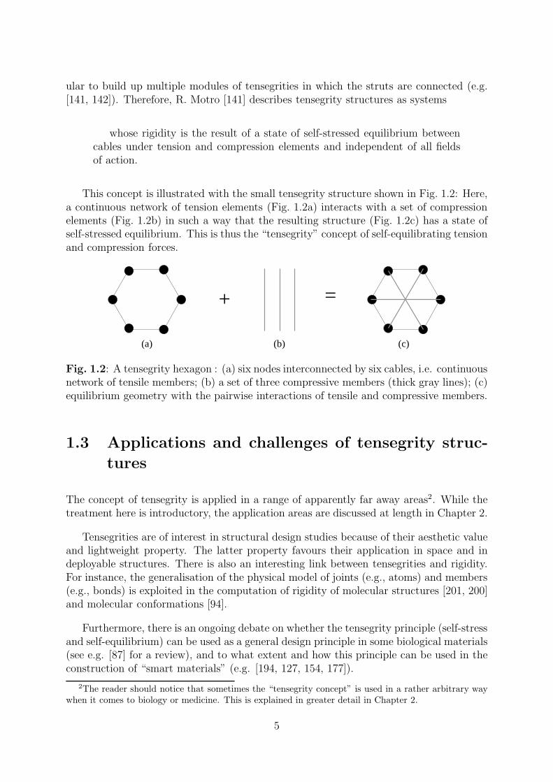
This concept is illustrated with the small tensegrity structure shown in Fig. 1.2: Here,a continuous network of tension elements (Fig. 1.2a) interacts with a set of compressionelements (Fig. 1.2b) in such a way that the resulting structure (Fig. 1.2c) has a state ofself-stressed equilibrium. This is thus the “tensegrity” concept of self-equilibrating tensionand compression forces.

+ =

(a) (b) (c)

Fig. 1.2: A tensegrity hexagon : (a) six nodes interconnected by six cables, i.e. continuousnetwork of tensile members; (b) a set of three compressive members (thick gray lines); (c)equilibrium geometry with the pairwise interactions of tensile and compressive members.

1.3 Applications and challenges of tensegrity struc-

tures

The concept of tensegrity is applied in a range of apparently far away areas2. While thetreatment here is introductory, the application areas are discussed at length in Chapter 2.

Tensegrities are of interest in structural design studies because of their aesthetic valueand lightweight property. The latter property favours their application in space and indeployable structures. There is also an interesting link between tensegrities and rigidity.For instance, the generalisation of the physical model of joints (e.g., atoms) and members(e.g., bonds) is exploited in the computation of rigidity of molecular structures [201, 200]and molecular conformations [94].

Furthermore, there is an ongoing debate on whether the tensegrity principle (self-stressand self-equilibrium) can be used as a general design principle in some biological materials(see e.g. [87] for a review), and to what extent and how this principle can be used in theconstruction of “smart materials” (e.g. [194, 127, 154, 177]).

2The reader should notice that sometimes the “tensegrity concept” is used in a rather arbitrary waywhen it comes to biology or medicine. This is explained in greater detail in Chapter 2.

5

There are a few fundamental problems associated to tensegrity structures standingalongside the many application areas. One essential problem is the initial geometry onwhich a tensegrity structure is based. The determination of the self-stressed equilibriumgeometry is known as form-finding, and it is discussed at length in this dissertation. Otherfundamental problems are about determining the mechanical behaviour of single tensegritymodules and their aggregation into larger structures. Together with this scalability issue,other problems arise like estimating the module’s stability, tolerance to manufacturingimperfections, and their active control of tensegrity with actuators. In all these aspects,many ideas that are now applied to tensegrity structures evolved from related fields dealingwith structures of a similar nonlinear geometrical behaviour.

The primary challenges related to tensegrity structures identified in this research aresummarised in the following points:

1. development of analytical form-finding methods with application to high-order tenseg-rity structures;

2. form-finding of arbitrary tensegrity structures (spheres, cylinders and asymmetricstructures) involving only minimal knowledge of the structure;

3. simultaneous form-finding and optimisation of system design parameters, for in-stance including constraints on member lengths and axial stiffnesses;

4. advancements in parameter identification and sensibility analysis to cope with ma-terial imperfections, as well as fabrication and assembly inaccuracies;

5. methods for faster form-finding of assemblies of known tensegrity units, e.g. capital-ising on essentially known units which are pile-up for tensegrity masts and tensegritygrids;

6. dynamics and control of tensegrity structures including folding, unfolding, activemembers and additional constraints of non-smooth character.

The research presented here focuses on the first two items of the list. It is entirelyrelated to form-finding issues, which without a proper treatment the remaining pointscannot be satisfactorily addressed. Form-finding is the first problem that should be rea-sonably solved to move on in tensegrity structures. The other items, although important,are left for future work.

Based on the current progress in mathematical and related numerical methods forcalculating tensegrity structures, the immediate future is likely to see important advancesin the aforementioned points. It is hoped that the present dissertation adds momentumto this effort.

6

1.4 State of the art of form-finding methods for tenseg-

rity structures

Form-finding is one of the basic problems in the design of any statically indeterminatestructures, and tensegrity structures are no exception. Tensegrity structures are not onlystatically, but often kinematically, indeterminate structures and require an initial form-finding procedure (e.g. [142, 191]). The form-finding process of tensegrity structures posesextra constraints. Detailed three-dimensional information is needed to create a state ofself-stressed self-equilibrium, that is, only pre-stress is considered.

Tensegrity structures only exist in a state of self-equilibrium, which requires the cal-culation of member forces in a particular spatial arrangement. To do so, mathematicalmodels and associated numerical algorithms have to represent nontrivial (i.e., nonzero)solutions for the member forces (i.e., tension or compression) in such a way that thestructure is stable. The resulting self-stressed self-equilibrium state is determined up toaffine and projective transformations. The geometry is due to the stress distribution ofthe self-stressed structure, which in the case of tensegrities is without the application ofexternal forces or anchorage points.

Form-finding methods for tensegrity structures typically compute a single critical pa-rameter that turns the structure to self-stressed equilibrium. That is, the calculatedstructures are normally described by a single unknown, which, if correctly estimated,causes the structure to be in self-stressed equilibrium. Therefore, some assumptions areplaced on the mathematical and mechanical models, e.g., a twisting angle, a strut-to-cablelength ratio, or a force-to-length ratio. The latter ratio is also known as the tension coef-ficient or the force density coefficient, a specification formalism which has been adoptedfor this dissertation.

A twisting angle is perhaps the easiest form-finding method for tensegrity structureslike the triplex and quadruplex, shown in Fig. 1.3. To shorten the names, the term n-plex is used for higher-order tensegrity cylinders. The triplex and quadruplex, 3-plex& 4-plex, have triangles and squares for constitutive polygons, shown in Fig. 1.3a andFig. 1.3c, respectively. The equilibrium configuration can be attained by calculating acertain twisting angle among the parallel polygons such that it causes the structure tohave a state of self-stressed self-equilibrium [51, 191, 185, 146, 145, 142, 96]. The heightof these cylinders is not explicitly defined by twisting angles, but it can be easily includedto get the final form in a subsequent step.

Other methods, however, predefine the length of all cables and iteratively elongate thestruts until the state of self-stressed equilibrium is found. This assumption again left onlyone parameter to be determined, i.e., the ratio of cable-to-strut length. Dynamic relax-ation [139] and nonlinear programming [157] approaches for the form-finding of tensegritystructures work in a similar manner. Interestingly, one analytical form-finding method[142] also exists, which also predefines cable lengths; however, it calculates the ratio di-rectly without involving any iterative process.

7

(b)(a)

(d)(c)

Fig. 1.3: Triplex and quadruplex : (a) connectivity of the triplex; (b) equilibriumgeometry; (c) connectivity of the quadruplex; (d) equilibrium geometry; the connectivityof (a) and (c) shows a continuous network of tensile members (black segments) and a setof compressive members (thick green lines).

In general, form-finding methods using tension coefficients tend to be more flexiblebecause they can describe single-parameter and multi-parameter self-stressed equilibriumgeometries [195, 196, 191]. A procedure, called force density method, is employed tocalculate the tension coefficients in the self-stressed state. It is typically analytical andcalculated with symbolic software. The number of different tension coefficients that par-ticipates in the form-finding is defined beforehand. However, a selection of only twodifferent tension coefficients is most popular: the first tension coefficient is normalised tobe unitary, while the second one is unknown. Then, the force density method calculatesthe reduced row echelon form of a force density matrix created with the tension coeffi-cients. An irreducible polynomial that produces a required rank deficiency is identified.The real roots of these polynomials provide the tension coefficients that cause the struc-ture to be in self-stressed equilibrium. Chapter 2 elaborates on this procedure as it is notrequired in our brief discussion here.

It is thus seen that each form-finding method, be it analytical or numerical, has note-worthy limitations. Each method is designed to work under certain narrow assumptionsor domain knowledge (see [142, 191] for a survey). Usually, to cope with a potentiallylarge number of unknowns, one or more of the following assumptions is used: elementlengths are predefined in dynamic relaxation and nonlinear programming procedures, aglobal symmetry is assumed in a group theory-based form-finding procedure, and/or arestricted number of different tension coefficients are imposed in symbolic analyses. Thelast constraint is used for the first part of the present dissertation.

Tensegrities like the 3-plex and 4-plex, shown in Fig. 1.3, have a characteristic equi-

8

librium configuration that appears in higher-order cylinders. A form-finding procedurestarts with a node-to-node connectivity (e.g., Fig. 1.3a or Fig. 1.3c), as well as certainconstraints, depending on the method employed, and calculate the equilibrium geometry(e.g., Fig. 1.3b or Fig. 1.3d). In the case of these two tensegrities, it is possible to do soby means of either twisting angles, strut-to-cable length ratios, or tension coefficients. Allthese approaches produce entirely equivalent solutions, i.e., the solution is basically thesame self-stressed equilibrium geometry.

Analytical solutions for the form-finding of tensegrity structures are known for smallsystems. They give some insights into parameter dependencies ; however, in general, theydo not extend to structures of both higher order and of difficult and generally multi-parameter forms. Modelling becomes worse for larger systems governed by assemblyof tensegrity units. In spite of many fine mathematical developments, the combinationof essentially known units is still extremely difficult, both theoretically and practically.The problems with respect to parameter dependencies and sensitivities concerning initialconditions include many open questions.

Numerical form-finding solutions, on the other hand, are generally achievable and, ascomputers become more powerful, they are less costly to obtain. Modelling and simulationare at the core of contemporary studies for tensegrity structures, not only for form-findingbut also for the study of the mechanical behaviour and sensitivity problems related totolerance to manufacturing imperfections. Capability in analysis will naturally lead totopology optimisation and later to shape finding. The investigations presented here area step forward in the analysis of tensegrity structures, and it is expected that additionaldesign information will be included in future form-finding methods.

1.5 Overview of the research

This dissertation presents analytical and numerical investigations of form-finding methodsfor tensegrity structures, with particular emphasis on cylindrical and spherical tensegritystructures.

The investigations cover triplex, quadruplex, truncated tetrahedron, expanded octa-hedron and truncated icosahedron structures, to name a few. The research is focused ontwo complementary form-finding methods, each with its own advantages and limitations.In the first one, the symmetry and a reduced number of different tension coefficientspose a certain constraint on the model that allows an analytical treatment of tensegritycylinders. A versatile numerical procedure is developed in the second investigation. Italleviates many assumptions and is thus far more general. The numerical form-findingprocedure is used to calculate both cylindrical and spherical tensegrities, as well as planartensegrities.

The detailed scope and driving questions that motivate both studies are described asfollows.

9

Analytical investigations

The first study presents a thorough analysis of tensegrity cylinders, e.g., the triplex,the quadruplex, and higher-order cylinders. The proposed form-finding procedure doesindeed exploit the inherent symmetry of these cylinders. In the course of the research,certain tensegrities were found to have more than one possible configuration out of thesame node-to-node connections. They are thus called equivalent or structurally identicalconfigurations. For instance, there are no other possible geometrical configurations forthe triplex or quadruplex, Fig. 1.3; however, there are two for pentaplex, as shown inFig. 1.4a-c. Figure 1.4b and 1.4c shows the two equivalent configurations for the 5-plexgenerated out of the same nodal connectivity, Fig. 1.4a. Interestingly, the 6-plex has onlyone configuration while the 7-plex has three. It is not, however, immediately obvious whyit is so.

(a)

(b)

(c)

?

Fig. 1.4: Form-finding of the pentaplex : (a) the connectivity of a pentaplex. There aretwo geometrically different configurations out of the same connectivity, and both config-urations are self-stressed; (b) first self-equilibrium geometry; (c) star-like arrangement ofthe second self-equilibrium geometry. The pentaplex (b) and (c) are said to be equivalentor structurally identical configurations. Thick green lines are struts.

As higher-order tensegrity cylinders are explored, several questions arise. For instance,it is possible to ask: (i) how many configurations exist for a certain cylinder? (ii) whatsort of differences do they have? (iii) is it just possible to select the best among the rangeof equivalent configurations? (iv) is the 5-plex shown in Fig. 1.4b better than one inFig. 1.4c? and (iv) in which sense is “best” or “better” defined?

Conventional assumptions on the form-finding procedures, e.g., the symmetry imposedon tensegrity cylinders, may not always be available or easy to estimate beforehand forother classes of tensegrities. There is a lack of reports describing general form-finding pro-cedures, which, for instance, could solve both cylindrical and spherical tensegrities. This

10

gap in the literature hinders the general applicability of existing form-finding methods,and thus tensegrity structures altogether.

Numerical investigations

In the second study, a form-finding procedure that provides solutions to most traditionalproblems is proposed. As exact analytical solutions become unmanageable for more com-plex structures, a numerical procedure was developed. Tension coefficients seem to bemore flexible and convenient for form-finding methods, in stark contrast to angles or ra-tios of member lengths. One problem in the path to numerical form-finding proceduresis the initialisation. Where does one start? If the number of assumptions is to be re-duced, it might be sensible to consider what “minimal” information one needs to start aform-finding method.

The lack of a priori information was identified and addressed by developing an uncon-ventional numerical form-finding procedure that only uses: the node-to-node connectionsand the sign of individual members as either tension or compression. 2D and 3D struc-tures, as well as symmetric and asymmetric cases for tensegrity cylinders, are discussed.

Tensegrity cylinders described in the analytical study study were re-calculated; how-ever, a restricted number of tension coefficients for the form-finding was not assumed.This leads to the question: (v) how many different tension coefficients can be calculatedfor a tensegrity cylinder? It is also natural to compare some aspects of both analytical andnumerical procedures. In particular, (vi) what is the accuracy of the numerical solutioncompared to the analytical one? Further, (vii) how does one search among equivalentconfigurations? Or, (viii) what are the (dis-)advantages of computing analytical andnumerical solutions? Is it worth computing a numerical solution?

So far, the area of form-finding has plenty of methods that require specific knowledgeof the final tensegrity structure. This introduces extra constraints to the user and hindersuncompromised designs. Never the less, as a result of the two investigations, previousand new tensegrity structures can easily be calculated and certainly opens the door tonovel designs. It is expected that these investigations will help to discover new struc-tures and provide starting points for future developments in the form-finding of staticallyindeterminate structures.

1.6 Outline of the dissertation

The dissertation is organised as follows. The terminology and equations used throughoutthe research are presented in Chapter 2. Some the many areas of application of tensegritystructures are briefly listed there. The overview in Chapter 2 is broad but self-containedto bridge the gap between apparently disconnected areas.

An analytical treatment for the form-finding of tensegrity cylinders is presented in

11

Chapter 3. Besides calculating the form-finding of tensegrity cylinders of non-equal cir-cular faces, the number of equivalent solutions is also counted and enumerated. In doingso, points (i) and (ii) are addressed in a purely geometrical, exact way.

Discussions on the stability and non-uniqueness of the analytical form-finding treat-ment of tensegrity cylinders are provided in Chapter 4. Point (ii) is dealt with an energycriterion. Further, points (iii) and (iv) are carried out with the principle of minimumstrain energy. The chapter also serves as an interface between the analytical and numericalform-finding studies by focusing on point (v).

A numerical form-finding method is fully described in Chapter 5. The solutions of thenovel iterative procedure were compared to other approaches. The chosen cases of studyare cylindrical and spherical tensegrity structures. Close attention was paid to points(vi) and (vii). Finally, conclusions drawn from both studies appear in Chapter 6. Theadvantages and disadvantages (point (viii)) of the analytical and numerical methods arediscussed in the final chapter.

12

Chapter 2

Tensegrity structures

A general overview of tensegrities, including the most important application areas, is pro-vided in this chapter. The terminology and equations used in this dissertation are alsodefined. It is important to remark that the nomenclature in the field of tensegrity struc-tures is not unified; nevertheless, an effort is made to adhere to [142] and [191]. Besides ageneral introduction to tensegrity structures, the information necessary to proceed withthe remaining chapters is presented here; for a larger overview, the reader is encouragedto consult [142].

The chapter is organised as follows. After presenting the basic hypotheses in Sections2.1 and 2.2, an overview of application areas is shown in Section 2.3. Equilibrium equationsof a general pin-jointed framework are provided in Section 2.4, and rank conditions for astructure having a state of self-stress are shown in Section 2.5. A calculation of the initialstiffness in statically indeterminate structures is provided in Section 2.6. A review of form-finding methods for tensegrity structures is presented in Section 2.7. The review focuseson the triplex as basic structure. Finally, a full example is presented in Section 2.8, withall main matrices, vectors, and calculations associated to the form-finding of the triplex.

2.1 Attraction and repulsion

Tensegrity structures are used to model a wide range of physical systems. What makestensegrity structures so general is the concept of balancing tension and compression in aclosed system. Because tensegrities are statically indeterminate structures1, their internalforces are nonzero and it focuses the interest on how the members balance their forces.There are many physical systems where the particles interact in such a way, resulting in a

1The term “statically indeterminate” seems to be introduced into English literature in the early 20thcentury, e.g. in the discussion of arch bridges over the Niagara river [110]. However, the problem inwhich the bar tensions are not uniquely determined by the equations of nodal equilibrium was firstpresented and solved by Navier [148], and shortly afterwards by Moseley, Poncelet, Maxwell and Mohr[37, 38, 40, 42, 95]. The term itself, “statically indeterminate”, is probably a direct translation from theGerman “statisch unbestimmt”, which is used since the late 19th century, e.g. [144].

13

self-equilibrated system. However, as can be seen later on, many applications of tensegritystructures use this formalism for more qualitative rather than quantitative guidelines.Moreover, in general, the selection of tensegrity structures in the fields of biology andmedicine seems to be based on empirical knowledge and very few measurements.

The key point in the tensegrity concept, i.e., balancing continuous tension and dis-continuous compression, can represent different varieties of physical models. In a generalsetting, tension and compression are replaced by attraction and repulsion, respectively.Interactions between nodes are assumed to be perfectly pointwise, insofar as these inter-actions are modelled with massless joints (i.e. nodes).

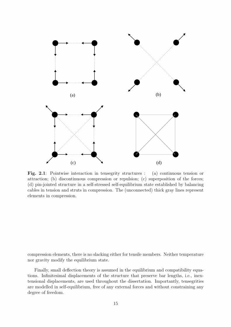
Figure 2.1 illustrates the interacting forces in a tensegrity structure. The continu-ous network of attraction (Fig. 2.1a) and discontinuous repulsion (Fig. 2.1b) acts uponone another (Fig. 2.1c) to keep a self-stressed self-equilibrium (Fig. 2.1d) configuration.Compression elements are shown as thick gray lines. Figure 2.1c shows the assembly oftension and compression between the nodes with pointwise interactions of attraction andrepulsion, respectively. The diagonal dotted lines in Fig. 2.1b or Fig. 2.1c do not touchor interfere with each other.

Figure 2.1d shows the wiring of this small tensegrity structure: tension forces arereplaced by cables and repulsion by struts (thick gray lines). There is no intersection inthe pair of struts shown in Fig. 2.1d. The scalar quantities for tension and compressionforces that self-equilibrate the structure Fig. 2.1d are not unique2, but a self-stressedself-equilibrium configuration is determined up to affine and projective transformations[59, 186]. The geometry of Fig. 2.1d is due to the balancing of forces, with no externalloads nor anchorage points.

2.2 Basic hypotheses

A number of basic assumptions should be clarified before presenting the mathematicalmodels and numerical algorithms used for the form-finding of tensegrity structures. It isconvenient to discuss the mathematical model as well as the limitations of the currentapproach.

Research on tensegrity structures normally idealises tensegrities in which the structuralmembers are held together by frictionless joints, and the self-weight of the structuralmembers is neglected. Strictly speaking, the idealised condition of frictionless and masslessjoints is, of course, never satisfied, but it is a simplification that helps in calculations andgives meaningful reference points. The members, either in tension or compression, areassumed to be made of isotropic linear-elastic materials. This assumption focus to theextremely narrow limit within which, in the case of ordinary materials, Hooke’s law issatisfied. A given member is either in tension or compression, i.e. a tension elementcannot support compression and vice versa. While there is no buckling considered for

2The solution for the internal forces of Fig. 2.1d is a vector t = α[1 1 1 1 − 1 − 1], with α for tensionand −α for compression; α can be an arbitrary positive (real) constant.

14

(a) (b)

(d)(c)

Fig. 2.1: Pointwise interaction in tensegrity structures : (a) continuous tension orattraction; (b) discontinuous compression or repulsion; (c) superposition of the forces;(d) pin-jointed structure in a self-stressed self-equilibrium state established by balancingcables in tension and struts in compression. The (unconnected) thick gray lines representelements in compression.

compression elements, there is no slacking either for tensile members. Neither temperaturenor gravity modify the equilibrium state.

Finally, small deflection theory is assumed in the equilibrium and compatibility equa-tions. Infinitesimal displacements of the structure that preserve bar lengths, i.e., inex-tensional displacements, are used throughout the dissertation. Importantly, tensegritiesare modelled in self-equilibrium, free of any external forces and without constraining anydegree of freedom.

15

2.3 Applications

Tensegrities are applied in a range of apparently disconnected areas. PubMed3 is a goodsource of articles on tensegrity in life sciences journals, or ISI Web of Science4 for a broadersearch. The interplay and arrangement of tension and compression show some interestingcharacteristics common to many prestressed structures, including living organisms, whichinclude:

• structures being able to fold and deploy,

• re-establishing geometry and stiffening due to the prestress, and

• lightweight structures because of the extensive use of tensile members.

While tensegrities are best known as space structures, there are little known areasin which the “tensegrity concept” is used as a guiding model. The quantitative andqualitative aspects of tensegrity structures are used in a broad class of problems. In manycases, interest is not on calculating an equilibrium geometry but in analysing structuresthat lose rigidity, or computing floppy modes. In the following, the main areas in whichtensegrities, or closely related concepts, play an important role are briefly reviewed.

Architecture and civil engineering

Tensegrities are of interest in structural design studies because of their lightweight prop-erty, aesthetic and modern look. Usually, the structures are built in such a way thatstruts are connected, which might not be the original definition for tensegrity.

It is interesting to mention the following developments, starting of course with themany designs by K. Snelson [178], tensegrity domes [17, 24, 86, 85, 90, 112, 119, 122,140, 149, 166, 173, 187, 189, 203], tensegrity bridges [44, 202], tensegrity towers [113, 64,161, 172], tensegrity glass-tower [11], antennas [73, 114, 115, 190], deployable tents [23],and architectural designs [120, 121, 122, 36]. This is the classical field in which tensegritystructures are applied, see [142] for a longer list of references.

Biology and chemistry

The current trend of applying tensegrity structures in biomechanics of cells and moleculesis helping researchers to qualitatively understand the structure-function relationship ofcells. Such an application also provides quantitative discrete cell models to researchers ofbiomechanics and tissue engineering. Because of the complexity of the material properties

3http://www.ncbi.nlm.nih.gov/entrez4http://isiknowledge.com

16

and the geometries encountered in applications, implementation of biomechanical modelsin numerical codes is vital. A common goal for those working in cell mechanics is toanalyse the causal connections and to make predictions based on abstraction and generalprinciples observed in adherent cells.

Ingber and co-workers, as well as a few other independent authors, have repeatedlypublished that some aspects of adherent cells can be qualitatively modelled with tensegri-ties, for instance cell spreading, motility and mechanotransduction [87, 97, 106, 107, 104,103, 102]. Cellular tensegrity models are employed to explain the balance of forces, themovements of organelles and the changes in cytoskeletons that start biochemical reac-tions [87, 108, 43, 81, 88, 150, 155, 5]. It is known that cells are mechanically less stable,and show reduced motility and migration by disturbing the cytoskeleton [75], which isexplained as a loss of rigidity in the cellular tensegrity model. Further, changes in cy-toskeleton, due to controlled physical distortion, are also associated to changes in cellgrowth and function, and these phenomena are said to be somehow explained with thecellular tensegrity model [98, 105, 108, 101, 100, 99].

However, with over a hundred publications in the field, a quantitative model for thecellular mechanical behaviour is yet to be seen. The validation of mathematical modelsoften requires careful laboratory experiments or testing; nevertheless, there are few quan-titative validations of the cellular tensegrity hypothesis. Some steps taken forward in thisdirection are the investigations done by some researchers [25, 26, 27, 55, 57, 56, 54] for themodelling of cytoskeleton of adherent cells. The author of this dissertation is not awareof any development on models of cellular tensegrities for motility and spreading.

Other biological models with links to tensegrity structures are related to the Caspar-Klug theory of virus structure or virus as minimum energy structures [29, 111, 128]. Otherauthors created DNA “tensegrity” structures [124] - a claim that is very debatable.

Tensegrity structures are also used for the qualitative modelling of the muscular-skeletal system [118, 152], which balances the forces of muscles (tension) and bones (com-pression).

There is also a fascinating link between tensegrities and rigidity. For instance, gener-alisation of the physical model of joints (e.g., atoms) and members (e.g., bonds) is used inthe computation of protein flexibility prediction [109, 164], and the rigidity of molecularstructures [200, 201] and molecular conformations [94].

Smart structures

Unlike “traditional structures”, the so called “smart structures” automatically react toloading activity. Smart structures use actuators and sensors to react and achieve a certaingoal, for instance structural stability or locomotion.

Diverse characteristics of tensegrity structures are used in this domain. For instance,a number of structures [70, 71, 72, 82, 83, 65, 6] that can withstand the loads in an

17

active way have been reported. Tantalisingly, the analysis of tensegrity structures canbe complemented with artificial intelligence methods to improve the accuracy of dynamicrelaxation methods and active structural control. Hence, it is called an “active structure”.

There is one interesting parameter study of “tensegrity fabric” [126, 127] for dampeningthe friction between this compliant surface and the fluid it moves through. The designspace remains largely unexplored but their preliminary study gave promising researchdirections.

Other active structures concentrate more on the control of tension elements, makingthem actuators that improve the overall stiffness and folding of the structure [61, 62, 63,138, 153, 156, 162, 175, 176, 181, 182, 183], one of which - a triplex with actuators -can lead to successful locomotor robots [154]. Other publications on the active controlof tension and compression elements are [16, 69, 33, 34, 35, 129, 130, 131, 132]. Finally,there is considerable amount of literature on the characterisation and optimisation ofparameters for the control and manoeuvring of tensegrity structures [2, 3, 4, 7, 1].

Other interesting applications

Tensegrities are guiding models for democratic collaboration and decision making [8,9, 170, 10, 184, 160]. An icosahedron is chosen to model hierarchy-free interaction ofpeople working toward a common goal. The model can allocate and distribute a numberof participants. A limited number of skilled persons collaborate on a certain project(incident tensile member on nodes), while only a few can lead and peer review otherprojects (compression between two nodes). This model is said to be free of hierarchybecause of the lack of a “top” or “bottom” in spherical tensegrities.

Tensegrity structures provide ideas for the folding and unfolding process of attachmentpads in hornet’s legs [84]. Other interesting applications are the modelling of multi-vehicle systems [151]; piezo-tensegrity, which is the coupling of tensegrity structures andelectrically active devices [28]; rigidity percolation [74, 50, 134]; and “afunctional” abstractmolecular architectures [68].

2.4 Geometry and tension coefficients

The terminology and equations used in this dissertation are presented here. It is importantto remark that the nomenclature in the field of tensegrity structures is not unified. Someareas, such as mathematical rigidity, use similar matrices and vectors; nevertheless, theway they are related to engineering concepts is not obvious. Within tensegrity structures,there is no standard way of representing the main symbols and equations. An effort ismade to adhere to [142] and [191].

Figure 2.2 is used to exemplify the equations of static equilibrium of an unconstrainedreference node i connected to nodes j and k by members i j and ik, respectively. The

18

y

i

j

k

li,k

li,j

yk

yi

yj

xjxixk x0

fi,k

fi,j

f exti,x

f exti,y

Fig. 2.2: Equilibrium of an unconstrained node : the unconstrained reference node iis connected to nodes j and k. The three nodes lie within a two-dimensional space, forclarity, but the equations are written for a three-dimensional space. Here fA,B is the forcebetween nodes A and B and lA,B is the length of member AB. The node i is in equilibriumwith nodes j and k, and external forces f ext

i,x and f exti,y .

equilibrium equations are given by:

(xi − xj)fi,j/li,j + (xi − xk)fi,k/li,k = f exti,x

(yi − yj)fi,j/li,j + (yi − yk)fi,k/li,k = f exti,y

(zi − zj)fi,j/li,j + (zi − zk)fi,k/li,k = f exti,z

(2.1)

where any member AB that connects any two nodes “A” and “B”, in Fig. 2.2, has aninternal force fA,B and a length lA,B; and f ext is the external force. A simplified linearisednotation qA,B = fA,B/lA,B known as tension coefficient5, or force density coefficient [123,171] is often used. Equation (2.1) can thus either be written as:

(xi − xj)qi,j + (xi − xk)qi,k = f exti,x

(yi − yj)qi,j + (yi − yk)qi,k = f exti,y

(zi − zj)qi,j + (zi − zk)qi,k = f exti,z

(2.2)

5Credited to Muller-Breslau and Weyrauch, see [38] pp. 9, 69 and 156; but nevertheless the term wasamply used and popularised by Southwell [179].

19

or as(qi,j + qi,k)xi − qi,jxj − qi,kxk = f ext

i,x

(qi,j + qi,k)yi − qi,jyj − qi,kyk = f exti,y

(qi,j + qi,k)zi − qi,jzj − qi,kzk = f exti,z .

(2.3)

The tensegrity structures analysed in this dissertation have a state of self-stress withunconstrained nodes in ℜd, and zero external load in d-dimensions. Let x = [x1 . . . xn]

T ,y = [y1 . . . yn]

T , and z = [z1 . . . zn]T be the vectors of Cartesian coordinates for n nodes in

the x-, y-, and z-axes, respectively. Here (⋆)T represents a transpose operation. It is usedan incidence matrix C ∈ ℜb×n, which has one row per member A B, and its columns Aand B have entries +1 and −1, respectively. Equivalently, the incidence matrix C = (ci j)is the b× n matrix defined by

ci j =

+1 if j is the initial node of member i,−1 if j is the terminal node of member i,

0 otherwise,

for all i = 1 . . .b members composed by pairs of nodes A B, in which A 6= B, seee.g. [14, 15]. Notice that the orientation A B or B A is irrelevant for the subsequentcalculations. With the incidence matrix C, the projected lengths, e.g. (xA − xB), in thex-, y-, and z-axes are therefore written in vector form as Cx, Cy, and Cz, respectively.

Let t ∈ ℜb be a vector of tension coefficients, with one entry for each of the b members.It is possible to write the matrix form of Eq. (2.2) by factorising the projected lengths inthe equilibrium matrix A ∈ ℜdn×b and a vector t of tension coefficients:

At =

CT diag(Cx)CT diag(Cy)CT diag(Cz)

︸︷︷︸

Equilibrium matrix

t = 0, (2.4)

where diag(⋆) is a square matrix with the vector (⋆) along its diagonal, and d = 3 for athree-dimensional structure. See [136] for more information on linear algebra.

Similarly, if tension coefficients of Eq. (2.3) are factorised, its matrix representationrelates a symmetric matrix D ∈ ℜn×n, known as the force density matrix (FDM), or stressmatrix in mathematics [46], and the nodal coordinates:

D[xy z] =(

CT diag(t) C)

︸︷︷︸

FDM

[xy z] = [0 0 0]. (2.5)

Equation (2.4) relates the projected lengths to tension coefficients, whereas Eq. (2.5)relates tension coefficients to nodal coordinates. Equation (2.5) has quadratic form

20

xDxt =∑

tij(xi − xj)2, where the sum is over the pairs of connected nodes {i, j}. Notice

that matrix D = (di j) can be written as:

di j =

−qi j if i 6= j,∑n

k 6=i qi j if i = j,0 if nodes i and j are not connected,

where qi j is a tension coefficient between nodes i and j. In Gaussian network models(e.g. [193]), a very similar matrix D is used to represent biological macromolecules withresidues of proteins (nodes) and bonds (bars) by introducing a cut-off distance for spatialinteractions.

A force density matrix D is also found in the literature as D = CTQC, where Q isthe diagonal matrix of t. When there is no risk of confusion the explicit representation,Eq. (2.5), is used in this dissertation.

The force density matrix D is symmetric, positive semi-definite. Notice D is the matrixof second order differences of the structure, known in other fields as discrete or combi-natorial Laplacian matrix [14, 15, 135]; in this case, a Laplacian computed with negativeand positive edge weights. The matrix D can be expressed, likewise in graph theory, bysubtracting weighted versions of the vertex degree and adjacency matrices. Interestingly,D is conceptually a Kirchhoff matrix with positive and negative conductances. Equationslike the force density matrix and equilibrium matrix are present in a variety of fields, andcould be bridged by the Tellegen’s theorem or similar formalisms [89]. Both equationscan be combined, for a 3D structure, in the next relation:

DDD

xyz

−


t = 0,

or, written in another way,

(I3 ⊗D)

xyz

− At = 0,

where the Kronecker tensor product, ⊗, is used to shorthand the notation. It isimportant to stress that, in the following sections, it is assumed however that neitherelement lengths, coordinates, nor tension coefficients are known a priori.

2.5 Rank conditions and nullity

Two necessary but not sufficient rank conditions have to be satisfied in a d-dimensionalstructure that is in a state of self-stress, e.g. [142, 91, 46]. The first one ensures theexistence of at least one state of self-stress, if

21

r = rank(A) < b, (2.6)

which is necessary for a non trivial solution of Eq. (2.4). This rank deficiency providesthe number of independent states of self-stress s = b − r ≥ 1 and the total number ofinfinitesimal mechanisms m = dn− r for a structure in d-dimensions, as explained in [20].

The structural parameters, s and total m, are related through the Maxwell’s rule6,which in 3D is:

3n− b− c = m− s,

with constraints c ≥ 6; recall that n is the number of joints and b the number of barsin the structure. However, the total number of mechanisms includes rigid-body motions,c ≥ 3 for 2D, and c ≥ 6 for 3D.

The values of s and m give us the common classification, e.g. [158], of structuresaccording to their degree of static and kinematic indeterminacy:

s = 0, m = 0 : Statically and kinematically determinate structure;

s > 0, m = 0 : Statically indeterminate and kinematically determinate structure;

s = 0, m > 0 : Statically determinate and kinematically indeterminate structure;

s > 0, m > 0 : Statically and kinematically indeterminate structure.

Tensegrity structures are statically, and often kinematically, indeterminate structures.To put it explicitly, statically indeterminate structures have at least one state of self-stress,and kinematically indeterminate structures have at least one mode of deformation which isnot a rigid-body motion, i.e. s > 0 and m > 0. For instance, the small tensegrity structurewith four nodes and six bars, Fig. 2.1d, is a statically indeterminate and kinematicallydeterminate structure with s = 1 and m = 0.

To clarify the terminology, henceforth, the symbol m will be associated to the to-tal number of infinitesimal mechanisms minus the rigid-body motions, unless otherwisestated. Thus, the parameter m corresponds to internal mechanisms. The number of statesof self-stress indicate the non-trivial solutions to the system of equilibrium equations. Thesecond rank condition is related to the semi-definite matrix D of Eq. (2.5) as follows:

rank(D) < n− d, (2.7)

for a geometric embedding into ℜd. For an embedding of maximal affine space [91, 46, 47,48] the largest possible rank of D is (n− d− 1) for a d-dimensional structure. Basically,

6The rule, which relates the number of necessary bars to make a framework stiff, b = 3n− 6, was infact presented by Mobius long before Maxwell [38]. The rule acquire its present form from the works ofBuchholdt et al. [18] and Calladine [20].

22

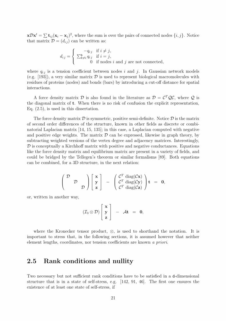
the nullity of D is (d + 1). The nullity of a matrix is the dimension of its nullspace: thenullity for a 2D structure is three, and the nullity for a 3D structure is four. The nullityof D is used in the form-finding procedure described in Chapter 5.

21(a)

1D

2D

3

1 2(b)

4

1 2

3D

3

(c)

Fig. 2.3: Rank conditions for the force density matrix : (a) the affine space of a line hasdimension two; (b) the affine space of a plane has dimension three; (c) the affine space ofa solid has dimension four.

An intuitive explanation of this rank condition is shown in Fig. 2.3. For instance, theaffine space spanned by a line has a dimension two (Fig. 2.3a), for a plane it is three(Fig. 2.3b) and for a geometric solid it is four (Fig. 2.3c).

From a graph-theoretical perspective, the form-finding problem basically consists in:computing edge weights such that the (weighted) Laplacian of the graph is positive semi-definite of certain nullity, and edge weights satisfy some pre-defined sign pattern fortension/compression elements. There are however some constraints on stability and nullitythat should be taken into account.

A degenerate configuration may exist in which, for example, three or more pointsare placed on the same straight line for a planar figure. That is, a planar figure maydegenerate in a line, which is of lower dimension. The numerical algorithms using thisrank condition, Eq. (2.7), should verify whether the nullspace really spans the expecteddimension without degeneracy. For instance, it could happen that the dimension of thenullspace of a 3D structure is four but one of the eigenvectors of this nullspace is the1-vector, with which the solid degenerates in a planar figure. The proposed form-findingprocedure discussed in Chapter 5 takes this maximal rank condition and nullity to find atensegrity structure.

2.6 Initial stiffness

Once a tensegrity structure is found, it is convenient to assess the stability of its self-equilibrium configuration. This configurations involves at least one state of self-stress

23

and infinitesimal mechanisms. It amounts to verify that [xy z] and t create a stableself-equilibrated structure in a kinematically indeterminate assembly. Or, in other words,the state of self-stress should stiffens all the infinitesimal mechanisms. Both tensioncoefficients and total number mechanisms are involved in this calculation.

Let [xy z] be the nodal coordinates of a structure in a state of self-stress, s ≥ 1. Itis known [159] that the basis of vector spaces of tension coefficients and mechanisms ofa self-stressed structure are calculated from the null spaces of the equilibrium matrix. Ifequilibrium matrix is factorised,

A =


= UVWT , (2.8)

the null spaces of Eq. (2.8) have the following structure,

U = [u1 u2 . . . |d1 . . . ddn−r], (2.9)

and

W = [w1 w2 . . . | t1 . . . tb−r], (2.10)

where r is the rank of the diagonal matrix V ; the vectors d ∈ ℜdn denote the m = dn− r

infinitesimal mechanisms; and the vectors t ∈ ℜb the states of self-stress, each of whichsolves the homogeneous Eq. (2.4). Let M ∈ ℜdn×dn−r be a matrix of mechanisms, M =[d1 . . . ddn−r], directly from Eq. (2.9), and possibly including the rigid-body motions. Bydefinition, the compatibility matrix (AT ) shows that mechanisms do not elongate anymember, i.e. ATM = 0.

Having calculated A and tension coefficients, Eq. (2.10), the tangent stiffness matrixis easily calculated. It is known that a vector of tension coefficients contributes to thetangent stiffness matrix,

Kt = Ke + Kg,= AGAT + (AQAT + I3 ⊗D),

(2.11)

of pre-stressed, kinematically indeterminate structures, see e.g. [93, 145]. Here Q is theb × b diagonal matrix of tension coefficients, G is the b × b diagonal matrix of axialstiffnesses, I3 is the 3x3 identity matrix, and ⊗ is the Kronecker tensor product.

If an infinitesimal and inextensional mechanism d ∈ M,M = [d1 . . . ddn−r] as de-scribed in Eq. (2.9), is applied to Kt, two terms Eq. (2.11) vanish, i.e. ATd = 0. Thestability of this initial state, or initial stiffness, of a structure therefore only involves, e.g.[145, 93, 197, 199], a section of the geometric stiffness: I3 ⊗ D. Stability of tensegrity

24

structures has been discussed not only from a mechanical point of view ([76, 67, 195, 198])but from a mathematical rigidity perspective ([48, 47, 46, 52, 51]). Other non-linear anal-ysis of tensegrity structures and affine systems close to singularities have been analysedin [12, 19, 66].

The infinitesimal mechanisms can be stiffened by the state of self-stress and this stiff-ness does not depend on the axial stiffness of the bars. Thus, the structure has an initialstiffness against load, and it is controlled by the level7 of pre-stress rather than the stiffnessof individual structural members.

The stability of a statically indeterminate pin-jointed structure in d = 3 dimensions,can be therefore tested with no other loads than its infinitesimal and inextensional mech-anisms. This can be done with the quadratic form of I3 ⊗D andM,

Λ =MT (I3 ⊗D)M, (2.12)

which is positive semi-definite if and only if D is positive semi-definite, for all m ∈ ℜdn.For a positive D, it has to be verified whether or not I3 ⊗ D, i.e. the reduced form ofEq. (2.11), imparts positive stiffness to all directions defined by the inextensional dis-placements except for the six rigid body motions,

eig(Λ) = [λ1 = λ2 = . . . λ6 = 0︸︷︷︸

rigid body motions

λ7 > 0 . . . λdn−r > 0︸︷︷︸

positive stiffness

], (2.13)

that appear in the analysis of free standing structures in d = 3 dimensions. Equation 2.13shows eigenvalues in increasing order and repeated according to their multiplicity. Here, itis assumed that there is a single state of self-stress, which is the typical example discussedin the related literature. In a general case, s ≥ 2, but nevertheless, is more problematic toverify whether or not the assembly possesses stiffness in all considered states of self-stress,e.g. [21, 22]. It is also possible that structures with s ≥ 2 have members that switchfrom tension to compression, depending of the state of self-stress. This fact introducesnew design problems because a member is not uniquely assigned a tension or compressionvalue. All structures presented in this dissertation avoid such a problem, each of themhas a single state of self-stress.

2.7 Form-finding of tensegrity structures

Form-finding methods for tensegrity structures typically compute a single critical param-eter that renders the structure to self-stressed equilibrium. That is, the structures beingcalculated are normally described by a single unknown which, if correctly estimated, causethe structure to be in self-stressed equilibrium. Therefore, some assumptions are placed

7A non-zero level of pre-stress that does not cause buckling in any member.

25

on the mathematical and mechanical models, for instance: a twisting angle, a strut-to-cable length ratio, or a force-to-length ratio. The latter ratio is also known as the tensioncoefficient or the force density coefficient, specification formalism which has been adoptedfor this dissertation.

A twisting angle is perhaps the easiest form-finding method for cylindrical tensegritystructures. The two triangles from which the triplex is composed are not aligned one overthe other. The equilibrium configuration is found by calculating a certain angle betweenthe parallel polygons such that it causes the structure to have a state of self-stressedself-equilibrium [51, 191, 185, 146, 145, 142, 96].

The twisting angle θ between the triangles of a 3-plex is θ = π/6, and, in general, theangle is

θ = π(

1

2− j

n

)

,

for any n-plex, e.g. [191, 142]; where 1 ≤ j < n/2, and n ≥ 3. The angle θ, createdbetween the parallel triangles of a triplex (Fig. 2.4a), is clearly seen in Fig. 2.4b. Thisparameter is normally assumed j = 1, however, the characteristics of n-plexes within therange 1 ≤ j < n/2 are largely unexplored. The relationship of j and n is not obvious,and it is clarified in the Chapters 3 and 4.

(a) (b)

Fig. 2.4: Form-finding with twisting angles : (a) equilibrium configuration of the triplex;(b) a top view shows the angle formed between both parallel triangles, adapted from [142],pp. 103.

Other form-finding methods, however, pre-define the length of all cables and iterativelyelongate the struts until the state of self-stressed equilibrium is found. This assumptionleft, again, only one parameter to be determined, e.g. the ratio between cable and strutlength. Dynamic relaxation [139] and non-linear programming [157] approaches for theform-finding of tensegrity structures work in such a manner8. Interestingly, there is also

8This form-finding method is closely related to the distance geometry formalism, with which current

26

one analytical form-finding method [142] that requires to pre-define the cable length butit calculates the ratio, directly, without involving any iterative process.

For instance, if the parallel triangles of a triplex are inscribed in circles of radii r =√

33

(Fig. 2.5a) and separated by a height h =

√3+3

√3

3, all tensile components have unitary

length, whilst all compression components have length ls =√

1 + 2√

33

, see Fig. 2.5b. Thisresult is essentially what other authors found for ls = 1.46788, e.g. [191].

r =√

3 / 3

(a) (b)

Fig. 2.5: Form-finding with length ratios : (a) unitary radius for the inscribed trianglesof the triplex; (b) the length of compression components is calculated by keeping unitarylengths in all tensile components; lc stands for cable length, lb is bracing cable length, andls is strut length.

In general, form-finding methods using tension coefficients tend to be more flexiblebecause they can describe single and multi-parameter self-stressed equilibrium geometries[195, 196, 191]. The procedure, called force density method, is typically analytical andemploys symbolic software. The number of different tension coefficients that participatesin the form-finding is defined beforehand. However, the selection of only two differenttension coefficients is most popular: the first tension coefficient being normalised to theunity and the second one is the unknown. Then, the force density method calculates thereduced row echelon form of a matrix, which is created with the tension coefficients. Incase of a triplex, the force density matrix D,

molecular structures can be calculated from the distances between bonded atoms. The distances arefound by experimental measurements and three-dimensional structures, consistent with them, have tobe calculated. Moreover, the distances are written in matrix form, in the same way as the item-itemdistance matrix used in classical multidimensional scaling.

27

D = CT QC =

2 −1 −1 q 0 −q

−1 2 −1 −q q 0

−1 −1 2 0 −q q

q −q 0 2 −1 −1

0 q −q −1 2 −1

−q 0 q −1 −1 2

,

has row echelon form,

2 −1 −1 q 0 −q

0 q −q −1 2 −1

0 0 0 3/2− 1/2 q2 0 1/2 q2 − 3/2

0 0 0 0 q2−3q

− q2−3q

0 0 0 0 0 0

0 0 0 0 0 0

;

where the diagonal matrix,

Q =

1 0 0 0 0 0 0 0 0 0 0 0

0 1 0 0 0 0 0 0 0 0 0 0

0 0 1 0 0 0 0 0 0 0 0 0

0 0 0 1 0 0 0 0 0 0 0 0

0 0 0 0 1 0 0 0 0 0 0 0

0 0 0 0 0 1 0 0 0 0 0 0

0 0 0 0 0 0 q 0 0 0 0 0

0 0 0 0 0 0 0 q 0 0 0 0

0 0 0 0 0 0 0 0 q 0 0 0

0 0 0 0 0 0 0 0 0 −q 0 0

0 0 0 0 0 0 0 0 0 0 −q 0

0 0 0 0 0 0 0 0 0 0 0 −q

,

assigns unitary tension coefficients to tensile components in the parallel triangles of thetriplex. Variables q and −q are unknowns for bracing cables and struts, respectively. Theincidence matrix C is explained in Section 2.8.

Irreducible polynomials that produce the required rank deficiency are identified fromthe row echelon form, shown previously. The real roots of these polynomials, e.g. q2−3

qfor

the triplex, provide the tension coefficients that cause the structure to be in self-stressed

28

1

6

3

4

2

5

45

6

12

3

(a) (b)

Fig. 2.6: A triplex : (a) six nodes being interconnected by nine cables and three struts;(c) equilibrium geometry with one state of self-stress

equilibrium, i.e. q =√

3. The correct nullity, four in this case, see Eq. (2.7), is found bylooking for the positive real roots. Chapters 3 and 5 elaborates on this procedure whichit is not need in our abbreviated discussion here.

2.8 Example: the triplex

Before moving on to the main part of this dissertation, it seems convenient to show onesmall example with all its main matrices and vectors. This section presents the tensioncoefficients, coordinates, force density and equilibrium matrices associated to the triplex.The coordinates and tension coefficients of the self-stressed solution are presented withno further explanation. They are derived in detail in Chapter 3.

The six nodes (n = 6) and their connections (b = 12) are shown in Fig. 2.6. Thistensegrity, Fig. 2.6, is called triplex and it is perhaps the smallest three-dimensionaltensegrity structure. It consists of two triangles, made of tensile components, connected bythree bracing cables and three struts. It is a well-known tensegrity structure, which Motro[142] also calls “elementary equilibrium” or “simplex”, and its equilibrium configurationcan be found by numerous form-finding techniques.

From the figure Fig. 2.6 it can be seen that there are twelve members, listed as follows:1 2, 2 3, 1 3, 4 5, 5 6, 4 6, 1 4, 2 5, 3 6, 1 5, 2 6, and 3 4; with no distinction for order A B orB A. The vectors x,y, z ∈ ℜn of Cartesian coordinates of the six nodes are as follows:

x = [1 −1/2 −1/2√

32−

√3

20]T ,

y = [0√

32−

√3

21/2 1/2 −1]T ,

z = [0 0 0 1 1 1]T .

29

The incidence matrix, C ∈ ℜb×n, shown in Eq. (2.14), has one row for each of thesetwelve pairs of nodes:

C =

1 2 3 4 5 6

1 −1 0 0 0 0

0 1 −1 0 0 0

1 0 −1 0 0 0

0 0 0 1 −1 0

0 0 0 0 1 −1

0 0 0 1 0 −1

1 0 0 −1 0 0

0 1 0 0 −1 0

0 0 1 0 0 −1

1 0 0 0 −1 0

0 1 0 0 0 −1

0 0 1 −1 0 0

. (2.14)

For clarity, the nodes (1-6) are indicated with labels at the top of the incidence matrixC, Eq. (2.14), in which the first row of C (from top to bottom) means a connection betweennodes 1 and 2; and only the columns of these pair of entries, 1 and 2, are non-zero. Theassociated tension coefficients are q = 1 for the six horizontal cables: 1 2, 2 3, 1 3, 4 5, 5 6,4 6; q =

√3 for each bracing cable cables: 1 4, 2 5, 3 6; and, finally, q = −

√3 for the three

struts: 1 5, 2 6, 3 4. Therefore, the vector t ∈ ℜb of tension coefficients is

t =[

1 1 1 1 1 1√

3√

3√

3 −√

3 −√

3 −√

3]T

.

Having calculated the incidence matrix C and the vector of tension coefficients t, theforce density matrix, or stress matrix in mathematics, is:

D = CT diag(t)C =

2 −1 −1 −√

3√

3 0

−1 2 −1 0 −√

3√

3

−1 −1 2√

3 0 −√

3

−√

3 0√

3 2 −1 −1√

3 −√

3 0 −1 2 −1

0√

3 −√

3 −1 −1 2

.

30

It is possible to verify that the nullity of D is four, and it satisfies Eq. (2.7). Fromthe equilibrium equations follows that Dx = fext

x = 0, Dy = fexty = 0, Dz = fext

z = 0.Actually, the coordinates [x,y, z] can be calculated by factorising D = UVUT , and lookinginto the leftmost eigenvectors in the unitary matrix U ; here the diagonal matrix V haseigenvalues [λ1 = λ2 = . . . λ4 = 0 λ5 = 6 λ6 = 6]. With the coordinates of the self-equilibrated configuration, the infinitesimal mechanisms are calculated by decomposingthe equilibrium matrix, A ∈ ℜ3n×b:

A =

32

0 32

0 0 0 1 −

√

32

0 0 1 +

√

32

0 0

−32

0 0 0 0 0 0

√

3−1

20 0 −

12

0

0 0 −32

0 0 0 0 0 −12

0 0 −

√

3−1

2

0 0 0√

3 0

√

32

−1 +

√

32

0 0 0 0

√

3+1

2

0 0 0 −

√

3 −

√

32

0 01−

√

3

20 −1 −

√

32

0 0

0 0 0 0

√

32

−

√

32

0 0 1/2 0 1/2 0

−

√

32

0

√

32

0 0 0 −1/2 0 0 −1/2 0 0

√

32

√

3 0 0 0 0 0

√

3−1

20 0 1 +

√

32

0

0 −

√

3 −

√

32

0 0 0 0 0 1 −

√

32

0 0 −

√

3+1

2

0 0 0 0 0 32

1/2 0 0 0 0

√

3+1

2

0 0 0 0 32

0 01−

√

3

20 1/2 0 0

0 0 0 0 −32

−32

0 0 −1 +

√

32

0 −1 −

√

32

0

0 0 0 0 0 0 −1 0 0 −1 0 0

0 0 0 0 0 0 0 −1 0 0 −1 0

0 0 0 0 0 0 0 0 −1 0 0 −1

0 0 0 0 0 0 1 0 0 0 0 1

0 0 0 0 0 0 0 1 0 1 0 0

0 0 0 0 0 0 0 0 1 0 1 0

,

in A = UVWT . It follows that At = fext = 0. The rank of A is 11, so it fulfils therank condition Eq. (2.6), i.e. it is rank deficient. The unitary matrices U ∈ ℜ18×18

and W ∈ ℜ12×12, see Eq. (2.8), contain the basis for mechanisms, Eq. (2.9) and tensioncoefficients, Eq. (2.10),respectively. For instance, the original vector of tension coefficientsis found in the right null space of W, i.e.

W = [w1 w2 . . . w11 | t],

meanwhile the left nullspace,

U = [u1 u2 . . . u11 |d1 d2 . . . d7],

contains the infinitesimal displacements that produce no bar elongation: ATdi = 0,moving along the mechanism. The eigenvalues of the quadratic form of mechanisms,M = [d1 d2 . . . d7], and the reduced stiffness matrix, I3 ⊗ D, show that six out of theseseven infinitesimal displacements exert no work,

eig(MT (I3 ⊗D)M) = [ 0 0 0 0 0 0︸︷︷︸

rigid−body

4.8 ],

31

and correspond to the six rigid-body motions, see Eq. (2.13). The seventh eigenvalueis positive (λ7 = 4.8), Summarising, the structure has n = 6, b = 12, s = 1 and m = 1;the sign test Eq. (2.13) shows only one infinitesimal mechanism of deformation producingpositive work: the state of self-stress stiffens the structure.

32

Chapter 3

Analytical form-finding of tensegritycylinders

After having presented the basic definitions and terminology, in the previous Chapter,here it is shown an analytical investigation of tensegrity cylinders. This first investigationfocuses on certain tensegrity structures that are quite well-known for long time, butnevertheless some basic features of these cylinders have not been investigated so far.Moreover, the set of tension coefficients that self-equilibrate a cylinder is analyticallyderived in a straightforward way, and it improves previous calculations in this field.

The current Chapter provides insights into three different aspects of these cylindricalstructures. Firstly, an analytical form-finding process is presented for tensegrity cylindersof equal and non-equal circular faces. The novel solution is shown in terms of tensioncoefficients and covers cylinders consisting of either convex or star polygons. Secondly,asymptotic analyses of lengths and forces in the cylinders are calculated as the numberof nodes used to discretise the circular faces tends to infinity. Thirdly, it is shown how tocount and enumerate all possible equivalent solutions for a given n.

The Chapter is organised as follows. A brief introduction to tensegrity cylinders ispresented in Sections 3.1 and 3.2. An analytical form-finding procedure is presented inSection 3.3. The asymptotic analysis of the tension coefficients and the enumeration ofsolutions are shown in Sections 3.5 and 3.4, respectively. A full example (Section 3.6) anda brief discussion of a possible implementation (Section 3.7) help to clarify the details inour form-finding method. Some conclusions of this Chapter are drawn in Section 3.8.

3.1 Tensegrity cylinders

As indicated in the previous Chapter, the form-finding process of cylindrical tensegrities,e.g. the triplex and the quadruplex [142], has been studied using several approaches.There are, basically, four major classes of solution procedures for the form-finding of

33

tensegrity cylinders: dynamic relaxation and cable-to-strut ratios [142], non-linear pro-gramming [157], twisting angles [185, 146, 145, 51, 191], and by calculating tension coef-ficients1 [79, 195, 196].

In a previous work, [79], a form-finding procedure for tensegrity cylinders was presentedin terms of tension coefficients, i.e. force divided by length. The solution, however, onlyconsidered equal circular faces, and there was no attempt to characterise the differentconfigurations. Circular and non-circular faces are covered in the present analysis.

3.2 Geometric arrangement of tensegrity cylinders

Convex cylinders

A tensegrity cylinder, e.g. the triplex and quadruplex [142], consists of two polygons whichare interconnected by a set of n bracing cables and n struts. Each polygon consists ofn ≥ 3 nodes, and each node is linked to three members in tension and one in compression.Two out of the three tensile members lie in the same polygon, and the third member,a bracing cable, joins both parallel polygons. Figures 3.1a and 3.1b show the triplex(n = 3) and the quadruplex (n = 4), respectively.

(b)(a)

Fig. 3.1: Some examples of well-known tensegrity cylinders : Thick green lines representelements in compression. (a) 3-plex; (b) 4-plex.

1The force-to-length ratio of a member, also known as force density coefficient, see the previousChapter or [142, 191] for the standard terminology followed in this Chapter.

34

Star-like cylinders : equivalent configurations

However, the design of a pentaplex, or 5-plex for short, has an extra degree of freedom.It has two possible geometrical arrangements for the five nodes on the circular ends, seeFig. 3.2. It can be seen that the five nodes (Fig. 3.2a) can be joined with a continu-ous network of cables following the labels and arrows in Figs. 3.2b-c. It is possible tojoin the sequence of nodes from “A” to “E” without any cut in two different geometricarrangements.

A A

C

(b) (c)(a)D C

E B

E B

D

Fig. 3.2: Connecting five nodes in the plane with a single curve : (a) nodes lying on acircumference; (b) convex pentagon; (c) star pentagon, see e.g. [58].

The connections seen in Figs. 3.2b-c are effectively equivalent and can be exchangedfrom one to the other by a continuous re-arrangement of the nodes. They are thereforecalled “equivalent” configurations in the remaining Sections.

The corresponding tensegrity cylinders appear in Figs. 3.3a-b. These cylinders are infact two equivalent configurations of the 5-plex, which can be seen from their labels. Allnodes of Fig. 3.3a and their connections actually exist in Fig. 3.3b.

For instance, a node “A” is connected with cables to “B” and “E”, while it is beingconnected with a bracing cable to “A′” and with a strut to “B′”. Both cylinders, Fig. 3.3aand Fig. 3.3b, are wired in the same way.

However, those cylinders differ in their geometric arrangement. A closed figure withn = 5 nodes connected by n members can be either a convex (Figs. 3.3c and 3.2b) or astar polygon (Figs. 3.3d and 3.2c), e.g. [58]. It is generated by successively connecting bystraight members every j-th of the n nodes lying on a circumference, in which 1 ≤ j < n/2.For instance, in the star polygon (Fig. 3.3d), a node “A” is connected to node “B” atj = 2 steps along the circumference (from “A” to “B” via “D” along the dotted line inanticlockwise direction), while in the convex polygon (Fig. 3.3c) these nodes are j = 1steps apart, in clockwise direction.

Thus, it can be seen that both 5plex shown in Fig. 3.4a and Fig. 3.4b have the followingconnections:

• The first pentagon has AB, BC, CD, DE, and EA.

35

D

D’

A’

A

B

B’

C’

C

E

E’

C B

D A

E

A’

B

A

B’

E’

C

E

C’

D’

D

E C

B A

D

(a) (b)

(d)(c)

Fig. 3.3: Two configurations for the pentaplex : (a) 5-plex, j = 1; (b) 5-plex, j = 2;(c) convex polygon with j = 1 and its circumcircle; (d) star polygon with j = 2 and itscircumcircle. The 5-plex with j = 1 and j = 2, (a) and (b), respectively, are equivalentconfigurations.

• The second pentagon has: A′B′, B′C ′, C ′D′, D′E ′, and E ′A′.

• The bracing cables are: AA′, BB′, CC ′, DD′, and EE ′.

• Finally, the struts are: AB′, BC ′, CD′, DE ′, and EA′.

A top view of Fig. 3.3 can help to visualise the cylinder. Figure 3.4 has been createdwith different tapering so as to provide easier reading of their labels. The connectionsin both Fig. 3.4a and Fig. 3.4b are exactly the same. That is why it is said that bothtensegrities are “equivalent” or “structurally identical” configurations.

36

D’

E’

E

A

D

C’

B

C

A’

B’

(a)

C’

A’

A

C

E’

D

E

D’

B

B’

(b)

Fig. 3.4: Labels of two 5plex : top view of the only two equivalent configurations of the5-plex. (a) with j = 1; (b) with j = 2.

Form-finding with tension coefficients

As explained in the previous Chapter, most form-finding studies of cylindrical tensegritystructures have concentrated on determining the twisting angle between the two polygonalfaces. However, the analytical solutions of the form-finding of tensegrity cylinders can alsobe expressed in terms of tension coefficients. It has been shown [195, 196] how a symbolicanalysis can be used to find the critical tension coefficients for struts and bracing cablesthat generate a state of self-stress. The procedure uses Gaussian elimination and rootextraction.

A similar form-finding method that seeks the rank deficiency of the equilibrium matrixis presented in [181]. Other form-finding method also uses root extraction of polynomials[174], involving polynomials of hundred terms and 2n+1 roots for a given n-plex. Althoughtheir proposed symbolic form-finding seems sound and complete, their procedure is verytime-consuming. cylinders. Moreover, it is not easy to write the general solution for anarbitrarily large cylinder or calculate cylinders with non-equal circular faces. An analyticalform-finding procedure by which the tension coefficients are obtained in a straightforwardway is introduced in the following Section.

3.3 Analytical form-finding procedure

Here it is described an analytical form-finding procedure for tensegrity cylinders in termsof tension coefficients that covers equal and non-equal circular faces. Similar geometricalmodels, like Fig. 3.5a, have been studied with other form-finding methods based on atwisting angle between the polygons, e.g. [51, 191, 185, 146, 145, 142, 96]. In a previous

37

work, an analytical form-finding procedure in terms of tension coefficients was derivedfor cylinders with equal-sized polygons [79]. This Section extends our study to cylindersconsisting of circumscribed polygons with non-equal radii. It doing so, it is shown thattension coefficients are more appropriate than twisting angles to gain further insights intotensegrity cylinders.

A cylinder, Fig. 3.5, has two polygons, each one with n ≥ 3 points placed on thecircumferences of radii r1 and r2, separated at height h. The circumferences are identicalup to a scale factor r1/r2. They consist of members connecting every j-th node lying onthe circumference (Fig. 3.5b), where 1 ≤ j < n/2. The six nodes, from pa to pf , shownin Fig. 3.5a, have the following cylindrical coordinates:

pa = [−r2 sin(

π jn

)

, r2 cos(

π jn

)

, 0]

pb = [r2 sin(

π jn

)

, r2 cos(

π jn

)

, 0]

pc = [r1 cos(

2 π jn

)

, r1 sin(

2 π jn

)

, h]

pd = [r1 cos(

2 π jn

)

,−r1 sin(

2 π jn

)

, h]

pe = [r2 sin(

3 π jn

)

, r2 cos(

3 π jn

)

, 0]

pf = [r1, 0, h].

(3.1)

The members in Fig. 3.5a have the following meaning throughout the Chapter: thesegment pfpa is a strut of length ls and tension coefficient qs; pfpb is a bracing cable oflength lb and tension coefficient qb; pfpc, pfpd are cables of length lc1 and tension coefficientqc1; pbpe, pbpa are cables of length lc2 and tension coefficient qc2. By convention, the signof a tension coefficient is negative for compression members (i.e. struts) and positive fortension members (i.e. all types of cables).

Equal circular faces

The equations of static equilibrium for the point pf , Eq. (3.1) and Fig. 3.5a, can be solvedby assuming, for simplicity but without loss of generality, that tension coefficients inadjacent horizontal cables (pfpd and pfpc) are unitary, i.e. qc1 = 1. In this Section equalcircular faces are assumed, i.e. r1 = r2, and it follows that qc2 = 1. The ratio of tapering,r1/r2, is of course unitary but it is explicitly shown since it will make clear the transitionfrom equal to non-equal circular faces. This normalisation, in qc1 and qc2, means one canscale all the tension coefficients up to a nonzero positive constant without affecting theself-equilibrium. After the normalisation, the equilibrium equations may have only oneunknown, say q, which is the tension coefficient that equilibrates both: strut and bracingcable at point pf . Since the cylinder is fully symmetric, the solution found for point pf

applies to all other points within the same polygon with radius r1. The simplificationyields q = qb = −qs. This simplification is clarified in Section 4.3. It can be verified thatthe static equilibrium equations are satisfied in the y− and z− directions for a referencenode pf . The equilibrium equation in the x-direction is

38

pf

pc

pa

pb

pd

xy

z

h

r1

r2

pe

j

Pc. . .

2

1

1

2

. . .

j

Pd

Pi

(a) (b)

Fig. 3.5: Self-equilibrium state of a tensegrity cylinder : (a) members connecting tworeference points, pf and pb. The thick gray lines represent members in compression; (b)cables connecting every j-th of the n nodes lying on the circumference (dashed line).

2 qr2 sin(

π j

n

)

+ 2 r1 cos(

2π j

n

)

− 2 r1 = 0,

with q being the only unknown. By solving for q one gets,

q = −

(

2 r1

(

cos(

π jn

))2 − 2 r1

)

r2

(

sin(

π jn

)) = 2r1

r2

sin(

π j

n

)

.

Thus, in order to self-equilibrate a tensegrity cylinder its horizontal cables must haveqc1 = 1, for bracing cables

qb = 2r1

r2

sin(

π j

n

)

, (3.2)

and for struts

qs = −2r1

r2

sin(

π j

n

)

. (3.3)

The tension coefficients are valid for cylinders with equal radii. It was mentioned thatin this case r1/r2 = qc1 = 1, and it follows from the equilibrium equations that qc2 = 1.This completes the set of tension coefficients necessary to self-equilibrate a tensegritycylinder with equal-sized circular faces, and it is equivalent to the formulation presentedin [79].

39

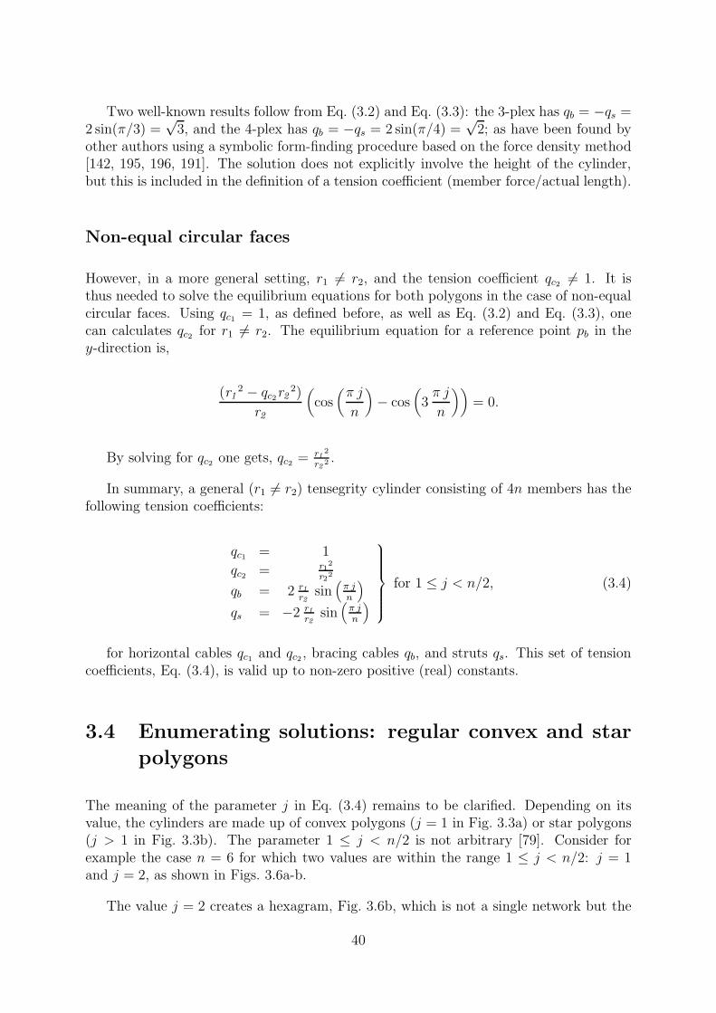
Two well-known results follow from Eq. (3.2) and Eq. (3.3): the 3-plex has qb = −qs =2 sin(π/3) =

√3, and the 4-plex has qb = −qs = 2 sin(π/4) =

√2; as have been found by

other authors using a symbolic form-finding procedure based on the force density method[142, 195, 196, 191]. The solution does not explicitly involve the height of the cylinder,but this is included in the definition of a tension coefficient (member force/actual length).

Non-equal circular faces

However, in a more general setting, r1 6= r2, and the tension coefficient qc2 6= 1. It isthus needed to solve the equilibrium equations for both polygons in the case of non-equalcircular faces. Using qc1 = 1, as defined before, as well as Eq. (3.2) and Eq. (3.3), onecan calculates qc2 for r1 6= r2. The equilibrium equation for a reference point pb in they-direction is,

(r12 − qc2r2

2)

r2

(

cos(

π j

n

)

− cos(

3π j

n

))

= 0.

By solving for qc2 one gets, qc2 = r12

r22 .

In summary, a general (r1 6= r2) tensegrity cylinder consisting of 4n members has thefollowing tension coefficients:

qc1 = 1

qc2 = r12

r22

qb = 2 r1

r2sin

(π jn

)

qs = −2 r1

r2sin

(π jn

)

for 1 ≤ j < n/2, (3.4)

for horizontal cables qc1 and qc2 , bracing cables qb, and struts qs. This set of tensioncoefficients, Eq. (3.4), is valid up to non-zero positive (real) constants.

3.4 Enumerating solutions: regular convex and star

polygons

The meaning of the parameter j in Eq. (3.4) remains to be clarified. Depending on itsvalue, the cylinders are made up of convex polygons (j = 1 in Fig. 3.3a) or star polygons(j > 1 in Fig. 3.3b). The parameter 1 ≤ j < n/2 is not arbitrary [79]. Consider forexample the case n = 6 for which two values are within the range 1 ≤ j < n/2: j = 1and j = 2, as shown in Figs. 3.6a-b.

The value j = 2 creates a hexagram, Fig. 3.6b, which is not a single network but the

40

(b)(a)

Fig. 3.6: Two different relationships of j for n = 6 : (a) the single connected curve isgenerated with j = 1; (b) two superimposed triangles generated with j = 2

superposition of two triangles. However, if j = 1 one can see that all n = 6 nodes areinterconnected and form a single network, Fig. 3.6a.

3.4.1 Possible configurations

In order to construct single connected networks, the relationship between n and j shouldbe such that the trigonometric angles (πj/n), in Eq. (3.4), generate single closed curvesembedded in two dimensions, e.g. [58, 169]. This is the case if j and n are relative primesor co-primes, which can be checked with the greatest common divisor (GCD), i.e. whenGCD(n, j) ≡ 1. Enumerating the solutions can thus be done by finding any 1 ≤ j < n/2being a co-prime to n. The following constraint is used in Eq. (3.4) to calculate thetension coefficients:

qc1 = 1

qc2 = r12

r22

qb = 2 r1

r2sin

(π jn

)

qs = −2 r1

r2sin

(π jn

)

for all 1 ≤ j < n/2 s.t. GCD(n, j) ≡ 1. (3.5)

Polygons satisfying this condition are visualised as single looped curves with n(j − 1)crossings, see Figs. 3.3c and 3.3d. The parameter j only affects the tension coefficients ofbracing cables and struts.

3.4.2 Counting the equivalent configurations

There are several equivalent solutions for most cylinders with n ≥ 3 and they are relatedto the aforementioned angle. For instance, the pentaplex has exactly two equivalentsolutions, Fig. 3.3a and Fig. 3.3b, but in general it is not obvious the number of equivalentsolutions for a larger n-plex.

41

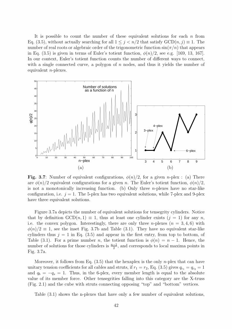
It is possible to count the number of these equivalent solutions for each n fromEq. (3.5), without actually searching for all 1 ≤ j < n/2 that satisfy GCD(n, j) ≡ 1. Thenumber of real roots or algebraic order of the trigonometric function sin(π/n) that appearsin Eq. (3.5) is given in terms of Euler’s totient function, φ(n)/2, see e.g. [169, 13, 167].In our context, Euler’s totient function counts the number of different ways to connect,with a single connected curve, a polygon of n nodes, and thus it yields the number ofequivalent n-plexes.

0 10 20 30 40 50 60 70 80 90 1000

5

10

15

20

25

30

35

40

45

50

Number of solutionsas a function of n

n−plex

φ(n)

/2

(a)

3 4 5 6 7 8 9

1

2

3

3−plex

4−plex

6−plex

(b)

Fig. 3.7: Number of equivalent configurations, φ(n)/2, for a given n-plex : (a) Thereare φ(n)/2 equivalent configurations for a given n. The Euler’s totient function, φ(n)/2,is not a monotonically increasing function. (b) Only three n-plexes have no star-likeconfiguration, i.e. j = 1. The 5-plex has two equivalent solutions, while 7-plex and 9-plexhave three equivalent solutions.

Figure 3.7a depicts the number of equivalent solutions for tensegrity cylinders. Noticethat by definition GCD(n, 1) ≡ 1, thus at least one cylinder exists (j = 1) for any n,i.e. the convex polygon. Interestingly, there are only three n-plexes (n = 3, 4, 6) withφ(n)/2 ≡ 1, see the inset Fig. 3.7b and Table (3.1). They have no equivalent star-likecylinders thus j = 1 in Eq. (3.5) and appear in the first entry, from top to bottom, ofTable (3.1). For a prime number n, the totient function is φ(n) = n − 1. Hence, thenumber of solutions for those cylinders is n−1

2, and corresponds to local maxima points in

Fig. 3.7a.

Moreover, it follows from Eq. (3.5) that the hexaplex is the only n-plex that can haveunitary tension coefficients for all cables and struts, if r1 = r2, Eq. (3.5) gives qc1 = qc2 = 1and qb = −qs = 1. Thus, in the 6-plex, every member length is equal to the absolutevalue of its member force. Other tensegrities falling into this category are the X-truss(Fig. 2.1) and the cube with struts connecting opposing “top” and “bottom” vertices.

Table (3.1) shows the n-plexes that have only a few number of equivalent solutions,

42

φ(n)/2.

φ(n)/2 n-plex1 3, 4, 62 5, 8, 10, 123 7, 9, 14, 184 15, 16, 20, 24, 305 11, 22

Table 3.1: Number of equivalent solutions for some tensegrity structures : The first rowshows that the 3-plex, 4-plex and 6-plex are tensegrity cylinders with only one possibleequivalent configuration, i.e. φ(n)/2 ≡ 1. The 5-plex, presented in Fig. 3.2 and Fig. 3.3,has two equivalent configurations. The 9-plex, analysed in Section 3.6 has three equivalentsolutions.

In summary, for a given n, all solutions that satisfy GCD(n, j) ≡ 1 are equivalentsolutions consisting of close looped curves with n(j − 1) crossings. A given n-plex hasφ(n)/2 ≥ 1 equivalent solutions. For j = 1, there are no crossings and the polygons areconvex. Any other solution not satisfying GCD(n, j) ≡ 1 corresponds to disconnectedpolygons.

3.5 Analysis of tension coefficients, forces and lengths

3.5.1 Tension coefficients

The analytical solution in terms of tension coefficients gives immediate access to forcesand lengths. Hence, one can analyse these asymptotic values when n or j approach theirlimits. A reader should be aware of inherent limitations of the small displacement theoryused in this work. The order of a tensegrity cylinder can be arbitrarily large, n → ∞,while j can be arbitrarily close to n/2. These limits have to be handled carefully insofarcertain forces and lengths tend to zero. The study of their asymptotic values is indeedimportant to understand the cylinders for large enough n.

The tension coefficients in the horizontal cables, qc1 and qc2 in Eq. (3.5), are unaffectedby any change in n or j. However, tension coefficients of bracing cables and struts inEq. (3.5) show an interesting limit value:

tension coefficient limit n→∞ limit j → n/2

qb = 2 r1

r2sin

(π jn

)

0 2 r1

r2,

qs = −2 r1

r2sin

(π jn

)

0 −2 r1

r2.

(3.6)

It is seen in Eq. (3.6) how tension coefficients in bracing cables and struts are zero

43

when n tend to infinity. Since the tension coefficients are defined as force divided bylength, it is indeed possible to explore the value of both forces and lengths. A Taylorexpansion of qb and qs in Eq. (3.6) shows that values of tension coefficients in bracing

cables and struts decrease inversely proportional to n: qb = −qs = 2 r1

nr2π j + O

(1n3

)

. On

the other hand, if one vary the parameter j → n/2 the tension coefficients tend to a finitevalue, as a ratio of the tapering. There is however one drawback for j → n/2 : strutscollide in the centre; the incircle is reduced with j, e.g. Fig. 4.6.

3.5.2 Lengths

The tension coefficients qb and qs in Eq. (3.4) have a graphical meaning. The value of

2 sin(

π jn

)

corresponds to the length of a horizontal cable formed by connecting any twoconsecutive nodes at j steps. This length is depicted in Fig. 3.5b and corresponds tothe length, after defining j, of the segment pfpc or pfpd. The lengths lc1 and lc2 growmonotonically for 1 ≤ j < n/2. The lengths for each member, calculated from thecoordinates Eq. (3.1), are defined as follows:

lc1 = 2 r1 sin(

π jn

)

lc2 = 2 r2 sin(

π jn

)

lb =

√

r21 + r2

2 + h2 − 2 r1 r2 sin(

π jn

)

ls =

√

r21 + r2

2 + h2 + 2 r1 r2 sin(

π jn

)

(3.7)

Notice that lc1 and lc2 , in Eq. (3.7), include a term 2 sin(

πjn

)

, which tends to zero for

large n, see Eq. (3.6). The length of horizontal cables is therefore zero when n tends toinfinity, inasmuch as the unstressed bar length, l0 = EAl/(ql + EA), tends to zero forthe same limit; here E is the elastic modulus in a bar with cross sectional area A andlength l = lc1 or l = lc2 . This limit, n → ∞, has to be handled carefully since it isnot physically meaningful to assume zero-length cables. The limit values are thus used toshow the tendency of lengths, Eq. (3.7), and tension coefficients, Eq. (3.6). The behaviouris certainly a decreasing length as a function of the number of nodes used to discretisethe circular faces.

3.5.3 Forces

Any member of the cylinder has bar force f = EA(l − l0)/l0, where E is the elasticmodulus, A the cross sectional area, and l0 the unstressed bar length. Member forces canbe calculated with the tension coefficients and lengths, Eq. (3.4) and Eq. (3.7) respectively.The definition of tension coefficient is force divided by length, q = f/l, thus the memberforces are:

44

fc1 = qc1lc1 = 2 r1 sin(

π jn

)

,

fc2 = qc2lc2 = 2r21

r2sin

(π jn

)

,

fb = qblb = 2 r1

r2sin

(π jn

)√

r21 + r2

2 + h2 − 2 r1 r2 sin(

π jn

)

,

fs = qsls = − 2 r1

r2sin

(π jn

)√

r21 + r2

2 + h2 + 2 r1 r2 sin(

π jn

)

,

(3.8)

where fc, fb and fs are forces in horizontal cables, bracing cables and struts, respec-tively. The terms like 2 sin

(π jn

)

, in Eq. (3.8), tend to zero as n increases, see Eq. (3.6).

Thus, the limit values for large n and large j of the member forces Eq. (3.8) are as follows:

force limit n→∞ limit j → n/2fc1 0 2r1

fc2 0 2r21

r2

fb 0 2 r1

r2

√

(r1 − r2)2 + h2

fs 0 −2 r1

r2

√

(r1 + r2)2 + h2

(3.9)

The decreasing trend for large n, i.e. zeros in Eq. (3.9), is due to the fact that terms

like 2 sin(

π jn

)

decrease inversely proportional to n.

The tendency of these member forces is interesting, but the limit value (i.e. zero force)should be handled carefully : it implies zero-length horizontal cables. Figure 3.8 showsthis decreasing trend of all member forces; here the y-axis has (logarithmic) arbitraryscale in newtons. A Taylor expansion of fb and fs, for n→∞, gives more details of thislimit value:

fb = −fs = 2r1 π j

r2 n

√

r21 + r2

2 + h2 + O(

1

n2

)

.

That is, member forces increase within the range 1 ≤ j < n/2, and higher-order termsdecrease with n.

In summary, the tension coefficients (forces divided by lengths) in both struts andbracing cables have the same magnitude and decrease with the order of a cylinder. Thetension coefficients in horizontal cables are unaffected by n or j. The force in any member(tension coefficient times length) rapidly decreases as n grows, but it increases with 1 ≤j < n/2. The limit value of member forces, for j → n/2, is a finite non-zero value. Forthe case j = 1, the larger n the better the circumference is approximated by a convexpolygon, and the distance between any pair of adjacent nodes in the horizontal planesdecreases as a function of n.

45

3 10 15 20 25 30 35 40 45 500.114

1.114

2.114

3.114

4.14

n−plex

Mem

ber

forc

es

horizontalcablesbracingcablesstruts

Fig. 3.8: Logarithmic plot of member forces versus n : Numerical calculation showinghow the member forces decrease monotonically with n. All cylindrical tensegrity struc-tures are calculated with r1 = r2 = h = 1.

3.6 A full example: the 9-plex

This Section develops the form-finding of a tensegrity cylinder, and illustrates the use ofequations presented so far. It has been chosen the 9-plex. The 9-plex consists of twoenneagons, i.e. 9-sided polygons, linked with nine bracing cables and nine struts. Allexamples of this cylinder have r1 = 1 and r2 = 2.

There are four possible, 1 ≤ j < 9/2, ways to wire the cylinders. A visual inspectionof the four options, depicted in Fig. 3.9, confirms that there are only three valid polygons,i.e. j = 1, 2, 4. Table 3.1 shows that there are three valid cylinders associated to the9-plex. The values of j can be calculated with the Euler’s totient function, φ(9)/2 = 3,directly without drawing the polygons.

The four polygons are listed as follows: j = 1 is the regular enneagon shown inFig. 3.9a; j = 2 and j = 4 are star enneagons shown in Fig. 3.9b and Fig. 3.9d; and j = 3is a nonagram composed of three equilateral triangles, shown in Fig. 3.9c.

A nonagram, j = 3, has no single curve connecting all nine points in the plane.It is straightforward to calculate which j, from the 1 ≤ j < 9/2, produces a valid,

46

(a) (b)

(c) (d)

Fig. 3.9: Connecting nine nodes on the plane : (a) j=1; (b) j=2; (c) j=3; (d) j=4.

fully connected polygon. A quick calculation of the greatest common divisor shows thatGCD(9,1) = GCD(9,2) = GCD(9,4) = 1, but GCD(9,3)=3. It is therefore clear that onlyj = 1, 2, 4 produce valid polygons and j = 3 produces a nonagram.

The form-finding of the three valid 9-plex is calculated with Eq. (3.5). All tensioncoefficients for the nine tensile elements in the circumference of radius r1 are qc1 = 1, andfor radius r2 are qc2 = 12/22 = 1/4. The other tension coefficients, for bracing cables (qb)and struts (qs), are listed below:

if j = 1, qb = −qs = 212sin(πj

n) = sin (π/9) = 0.3420


n) = sin (2π/9) = 0.6427


n) = sin (4π/9) = 0.9848

(3.10)

Figure 3.10 shows the three valid configurations for the 9-plex, all of them derived fromthe same node-to-node connectivity. That is why Figs. 3.10a-c are said to be equivalentconfigurations from a connectivity point of view. The tension coefficients are the oneslisted in Eq. (3.10).

47

(a) (b)

(c)

Fig. 3.10: Three possible solutions for the 9-plex : (a) j=1; (b) j=2; (c) j=4. Allconfigurations are actually derived from the same nodal connectivity, i.e. equivalent, theonly variation is the parameter j of Eq. (3.5). One state of self-stress is found in allcylinders.

Advantages of the presented form-finding method are better appreciated when a com-parison with other methods based on tension coefficients is shown. A symbolic form-finding procedure based on the force density method is presented in [142, 195, 196]. Inorder to obtain the tension coefficients that self-equilibrate a cylindrical tensegrity struc-ture, the authors look for the positive real roots of a minimal polynomial that annihilatesa force density matrix, calculated with q = qb = −qs which is the only unknown; here itis assumed qc1 = qc2 = 1. It implies r1 = r2 = 1, or in other words, a cylinder with equalcircular ends.

48

A search of the abovementioned polynomials requires the solution of a system of linearequations: a force density matrix with dimensions 2n×2n. To start with, the force densitymatrix D = CT diag(t)C has

t = [1, . . . , 1, q, . . . , q, 1, . . . , 1,−q, . . . ,−q], (3.11)

and it is symbolically reduced to row echelon form. The procedure works with the as-sumption qb = −qs and qc1 = qc2 = 1, that is why t, Eq. (3.11), consists of four sections,with nine entries each one. From left to right, the vector t is:

t = [qc1 , . . . qc1 , q, . . . , q, qc2, . . . qc2,−q, . . . ,−q].

By determining the irreducible factors, one can see that the polynomial,

q8 − 9 q6 + 27 q4 − 30 q2 + 9 = 0,

has positive real roots: 0.6840, 1.2855, 1.7320, 1.9696; which are the same valuesobtained by applying Eq. (3.5). However, Eq. (3.5) provides a direct way to calculatethe tension coefficients. That is, if r1 = r2 it follows from Eq. (3.5), that: qb = −qs =2 sin (π/9) = 0.6840, qb = −qs = 2 sin (2π/9) = 1.2855, qb = −qs = 2 sin (4π/9) =1.9696. A set of values which can be seen in Table 3.2. The missing root, 1.7320, is infact 2 sin(3π/9) with which comes from a non-valid cylindrical tensegrity structure, i.e.j = 3 and n = 9.

It is interesting to notice that Eq. (3.5) selects the valid cylinders, which in the symbolicform-finding method has to be verified after the echelon form and root extraction. Itis also convenient to remark that our solution covers equal and non-equal circular faces:qc2 = r2

1/r22. Further, solutions obtained with the symbolic form-finding method described

above leave us with no clue about j, which influences the geometry, i.e. convex or star-likecylinders.

3.7 Implementation

This Section shows a piece of code that calculates the critical tension coefficient in strutsand bracing cables that self-equilibrate a tensegrity cylinder. The code, written for Maple,has no intention to be a definite guide in how to implement Eq. (3.5) and has no claimof good coding style. It calculates qb, which is equal to −qs. Tension coefficients on theparallel, circular faces are not calculated since qc1 = 1 for normalisation reasons, and qc2 isstraightforward, i.e. qc2 = r2

1/r22. The code is shown in Fig. 3.11, and it uses the package

of number theory (line 1).

The procedure accepts two parameters, the order of our tensegrity cylinder n and theratio r of the circular faces r1/r2, see line 3. It basically searches for all φ(n)/2 equivalent

49

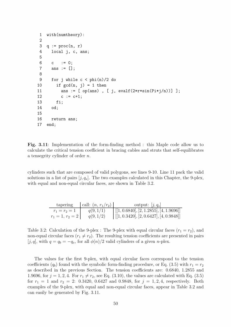
1 with(numtheory):

2

3 q := proc(n, r)

4 local j, c, ans;

5

6 c := 0;

7 ans := [];

8

9 for j while c < phi(n)/2 do

10 if gcd(n, j) = 1 then

11 ans := [ op(ans) , [ j, evalf(2*r*sin(Pi*j/n))] ];

12 c := c+1;

13 fi;

14 od;

15

16 return ans;

17 end;

Fig. 3.11: Implementation of the form-finding method : this Maple code allow us tocalculate the critical tension coefficient in bracing cables and struts that self-equilibratesa tensegrity cylinder of order n.

cylinders such that are composed of valid polygons, see lines 9-10. Line 11 pack the validsolutions in a list of pairs [j, qs]. The two examples calculated in this Chapter, the 9-plex,with equal and non-equal circular faces, are shown in Table 3.2.

tapering call: (n, r1/r2) output: [j, qs]r1 = r2 = 1 q(9, 1/1) [[1, 0.6840], [2, 1.2855], [4, 1.9696]]

r1 = 1, r2 = 2 q(9, 1/2) [[1, 0.3420], [2, 0.6427], [4, 0.9848]]

Table 3.2: Calculation of the 9-plex : The 9-plex with equal circular faces (r1 = r2), andnon-equal circular faces (r1 6= r2). The resulting tension coefficients are presented in pairs[j, q], with q = qb = −qs, for all φ(n)/2 valid cylinders of a given n-plex.

The values for the first 9-plex, with equal circular faces correspond to the tensioncoefficients (qb) found with the symbolic form-finding procedure, or Eq. (3.5) with r1 = r2

as described in the previous Section. The tension coefficients are: 0.6840, 1.2855 and1.9696, for j = 1, 2, 4. For r1 6= r2, see Eq. (3.10), the values are calculated with Eq. (3.5)for r1 = 1 and r2 = 2: 0.3420, 0.6427 and 0.9848, for j = 1, 2, 4, respectively. Bothexamples of the 9-plex, with equal and non-equal circular faces, appear in Table 3.2 andcan easily be generated by Fig. 3.11.

50

3.8 Conclusions and final remarks

This Chapter presented a form-finding procedure and a comprehensive analysis of cylin-drical tensegrity structures (n-plexes), in which the circular faces are composed of eitherconvex or star polygons. The circular faces consists of polygons created by connectingevery j-th node lying on their circumference. The analysis is done on the basis of ten-sion coefficients, and allows to calculate them directly in analytical way. The analyticalinvestigations permit to address the following issues at once:

Firstly, a solution for any n-plex, with equal and non-equal circular faces, is easilycalculated in closed-form. Tension coefficients, i.e. force divided by length, were usedinstead of twisting angles. For cylinders with equal circular faces our solution agrees withprevious studies. Tension coefficients that self-equilibrate the cylinders can be calculatedfor an arbitrarily large n-plex.

Interestingly, as a historical note, a tension coefficient like 2r sin(π/n), can easily bededuced from a paper [180] that deals with tubular frameworks for aeroplane fuselages;here r is the radius of the framework. The paper, published in 1933, develops a procedurefor the calculation of stresses in tubular frameworks and it is, to our best knowledge,the first use of tension coefficients similar to 2r sin(π/n) in mechanics. In his analysis,however, Southwell assumed that every bar in the framework can sustain both tension orcompression.

Secondly, it is possible to choose between convex (j = 1) and star-like (j > 1) cylinders.The equations developed for the form-finding introduce a parameter j with which a switchin the appearance of the n-plex is allowed. In fact, each circular face is visualised as singlelooped curves with n(j − 1) crossings

Thirdly, the enumeration of all valid j, coming from structurally identical n-plexes,generated out of the same n, is accomplished with the greatest common divisor. Theconfigurations are indexed by a parameter j that changes the geometric arrangement ofthe nodes. All tensegrity cylinders have at least one valid j, in which j = 1 correspondsto convex cylinders.

Finally, it is also possible to count the total number of equivalent configurations. Thenumber of these equivalent configurations is given by the Euler’s totient function, whichis not a monotonically increasing function with n, and its upper bound is a linear functionof n. It is also possible to count and show solutions having exactly certain number ofequivalent configurations. One interesting result of our analysis is that only three cylinders(n = 3, 4, 6) have no equivalent star polygons. The hexaplex deserves special attentionbecause it is the only n-plex that can sustain unitary tension coefficients, i.e. the valuesof axial force and length per member are equal, in all members.

51

Chapter 4

Stability and non-uniqueness of thesolution for tensegrity cylinders

The previous Chapter presented an analysis of cylindrical tensegrity structures. Theform-finding of cylindrical tensegrity structures was analytically derived using tensioncoefficients. An analysis of these structures shows that a number of solutions existsfor almost any n-plex. A number of geometrically different but equally valid cylindersproduced with the same connectivity, nodes and members was calculated. There areactually φ(n)/2 equivalent solutions for any n-plex. However, it is not clear a priori whatthe differences or properties are among all φ(n)/2 equivalent configurations per n. Theremust be a difference other than geometry. This Chapter presents further analytical butalso numerical studies that shed light into their differences.

The current Chapter provides insights into three different aspects of cylindrical tenseg-rity structures. Firstly, an analysis of their elastic strain energy is used to classify a numberof equivalent configurations that are generated out of the same n-plex. It is shown that thestrain energy attains its minimum at a state corresponding to convex cylinders, and showhow this energy is related to mathematical concepts of rigidity. Secondly, it is shown howthe analytical form-finding solution in terms of tension coefficients is non-unique. Thetypical assumption of having a reduced set of different tension coefficients is relaxed. Indoing so, asymmetric cylinders are created in such a way that all tension coefficients aredistinct from each other. Thirdly, the initial stiffness of these cylinders show that theirsingle state of self-stress stiffens all internal mechanisms. A full example, the 30-plex, ispresented to illustrate the concepts developed in this Chapter.

4.1 Introduction

In the previous Chapter φ(n)/2 equivalent solutions of the form-finding procedure wereshown for every n-plex. It is not clear a priori in which properties other than the geometricarrangement of their nodes, they differ. In order to investigate their differences, the elastic

52

potential energy of these equilibrium configurations is analysed. Global equilibrium isattained in the state of least energy. Therefore configurations with less potential energyare preferred to other local minima with higher value.

The analytical form-finding procedure, presented in the previous Chapter, introduced atypical but unnecessary simplification. A geometrical model was based on three differentelements: horizontal cables, bracing cables and struts. Since the tension coefficient inbracing cables and struts are identical scalar quantities, the set of tension coefficients isreduced by symmetry to horizontal and vertical members.

Moreover, if equal-sized faces are requested, the tension coefficients of all horizontalmembers are unitary. It leaves only one unknown to be calculated. However, all these sim-plifications are not necessarily. Tensegrity cylinders can be calculated in such a way thatall members have a different tension coefficient from each other. The inherent symmetryof the tension coefficients can be eliminated: no more parallel polygons, the equilibriumfor a single node does not copy to all other nodes by symmetry, member lengths are nolonger equal, &c.

Henceforth, the term “asymmetric” will refer to configurations having as many dif-ferent tension coefficients as members, i.e. there are no discernible groups of tensioncoefficients. The cylinders lose their symmetry in the tension coefficients, geometry andlengths. The non-uniqueness of the analytical form-finding procedure for tensegrity cylin-ders is thus discussed by presenting examples of asymmetric configurations.

Other authors have shown that tensegrity cylinders have a single state of self-stress[185, 142, 191]. However little is known on whether or not asymmetric star-like cylindershave a state of self-stress at all or if their self-equilibrium is stable. An analysis of theinitial stiffness allow us to to classify the equilibrium of cylinders. Finally, the relation-ship between initial stiffness and related mathematical concepts is briefly discussed. Forexample, what does a concept like “global rigidity” mean in engineering terms, and towhat extent and how this concept relates to structural stability. The present analyticalstudy contributes to fill this conceptual gap.

This Chapter is organised as follows. The calculation of the state of global equilib-rium is shown in Section 4.2. Asymmetric configurations and their initial stiffnesses arediscussed in Section 4.3 and 4.4, respectively. A full example, the 30-plex, is presented inSection 4.5. Finally, some conclusions of this work appear in Section 4.6.

4.2 Stability and global equilibrium

As previously shown in Section 3.4.2, there are φ(n)/2 structurally identical solutions outof the same n-plex, and it is not clear whether or not their equilibrium is similar. Toaddress this question, an elastic strain energy is assigned to each of these solutions. Theenergy is based on the pre-strain level in the members. This strain energy correspondsto the total elastic energy that is stored in the pre-stressed members of a tensegrity

53

cylinder. Assuming that all members, in all φ(n)/2 equivalent solutions for the same n,are made of the same material and have the same cross sectional area: a comparisonof their elastic strain energy allows to distinguish the structures on the ground of theprinciple of minimum strain energy, which is a particular case of the principle of leastaction. A derivation of the elastic strain energy follows.

Elastic strain energy

The elastic strain energy of a (cylindrical) tensegrity structure is calculated by describingits members as Hookean springs that store elastic energy upon experiencing a pre-strainε. Let ei, εi and ai be the Young’s modulus, the strain and the cross-sectional area of thei-th member, respectively. Then, if the stress and length of the i-th member are describedas σi = eiεi and li, respectively, the strain energy per unit volume of a structure is givenby:

U =1

2

4n∑

i=1

σiεi =1

2

4n∑

i=1

eiε2i =

1

2

4n∑

i=1

ei(fi

eiai)2 =

1

2

4n∑

i=1

f 2i

eia2i

=1

2

4n∑

i=1

l2i q2i

eia2i

. (4.1)

Here, each sum is taken over all 4n members of any cylindrical tensegrity structure, and fi

is the axial force of the i-th member. If the elastic strain energy of two or more structuresis compared, with the same Young’s modulus and cross-sectional area per member, thestrain energy Eq. (4.1) is just U ∝ ∑4n

i=1 l2i q2i . For clarity, the strain energy for a given

n-plex at configuration j, with member lengths (ln,j) and tension coefficients (qn,j), iswritten as follows:

Un,j ∝ n(ln,jc1

)2q2c1

+ n(ln,jc2

)2q2c2

︸︷︷︸

horizontal cables

+ n(ln,jb )2(qn,j

b )2

︸︷︷︸

bracing cables

+ n(ln,js )2(qn,j

s )2

︸︷︷︸

struts

. (4.2)

Please recall that tension coefficients in horizontal cables, i.e. qc1 and qc2 , are notaffected by the parameter j. The components of the analytical expression Eq. (4.2),involving squared tension coefficients and lengths for any n and j, are listed as follows:

q2c1 = 1

q2c2 = r1

4

r24

(qn,jb )2 = (qn,j

s )2 = 4 r12

r22

(

sin(

π jn

))2

(ln,jc1

)2 = 4 r12

(

sin(

π jn

))2

(ln,jc2

)2 = 4 r22

(

sin(

π jn

))2

(ln,js )2 = r1

2 + r22 + 2 r1 r2 sin

(π jn

)

+ h2

(ln,jb )2 = r1

2 + r22 − 2 r1 r2 sin

(π jn

)

+ h2.

(4.3)

54

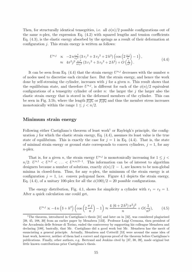
Then, for structurally identical tensegrities, i.e. all φ(n)/2 possible configurations out ofthe same n-plex, the expression Eq. (4.2) with squared lengths and tension coefficientsEq. (4.3), is the elastic energy absorbed by the springs as a result of their deformation atconfiguration j. This strain energy is written as follows:

Un,j ∝ −2 n r12

r22 (3 r1

2 + 3 r22 + 2 h2)

(

cos(

2 π jn

)

− 1)

,

≈ 4π2j2 r12

nr22 (3 r1

2 + 3 r22 + 2 h2) + O

(1n2

)

.(4.4)

It can be seen from Eq. (4.4) that the strain energy Un,j decreases with the number nof nodes used to discretise each circular face. But the strain energy, and hence the workdone by self-stressing the cylinder, increases with j for a given n. This result shows thatthe equilibrium state, and therefore Un,j , is different for each of the φ(n)/2 equivalentconfigurations of a tensegrity cylinder of order n: the larger the j the larger also theelastic strain energy that is stored in the deformed members of the cylinder. This canbe seen in Fig. 3.5b, where the length pfpc or pfpd and thus the member stress increasesmonotonically within the range 1 ≤ j < n/2.

Minimum strain energy

Following either Castigliano’s theorem of least work1 or Rayleigh’s principle, the config-uration j for which the elastic strain energy, Eq. (4.4), assumes its least value is the truestate of equilibrium. This is exactly the case for j = 1 in Eq. (4.4). That is, the stateof minimal strain energy or ground state corresponds to convex cylinders, j = 1, for anyn-plex.

That is, for a given n, the strain energy Un,j is monotonically increasing for 1 ≤ j <n/2: Un,1 < Un,2 < . . . < Un,n/2−1. This information can be of interest to algorithmdesigners because a number of solutions, exactly φ(n)/2 − 1, are known to be non-globalminima in closed-form. Thus, for any n-plex, the minimum of the strain energy is atconfiguration j = 1, i.e. convex polygonal faces. Figure 4.1 depicts the strain energy,Eq. (4.4), of a unitary 100-plex for all the φ(100)/2 = 20 possible configurations.

The energy distribution, Fig. 4.1, shows for simplicity a cylinder with r1 = r2 = 1.After a quick calculation one could get,

Un,j ∝ −4 n(

3 + h2) (

cos(

2π j

n

)

− 1)

≈ 4 (6 + 2 h2) π2j2

n+ O(

1

n2), (4.5)

1The theorem, introduced in Castigliano’s thesis [31] and later on in [32], was considered plagiarised[39, 45, 188, 30] from an earlier paper by Menabrea [133]. Professor Luigi Cremona, then president ofthe Accademia delle Scienze di Torino, ended the controversy by supporting his colleague Menabrea anddeclaring [188], basically, that Mr. Castigliano did a good work but Mr. Menabrea has the merit ofenunciating a general principle. Actually, Menabrea and Cotterill [53] were around the same idea ofleast work, however, neither of them had a correct and rigorous proof of the theorem before Castigliano’spublications. Finally, other authors, e.g. Bertrand and Jenkins cited by [37, 38, 39], made original butlittle known contributions prior Castigliano’s thesis.

55

1 3 7 9 11 13 17 19 21 23 27 29 31 33 37 39 41 43 47 49

3.15

500

1000

1500

2000

2500

3000

P a r a m e t e r j

Str

ain

ener

gy p

er u

nit v

olum

e (J

/m3)

Unitary 100−plex

Fig. 4.1: Elastic strain energy : possible configurations j of a unitary 100-plex, i.e.r1 = r2 = h = 1. A minimum strain energy is attained at j = 1, which is the tensegritycylinder with convex faces.

which shows the energy Eq. (4.5) proportional to j, for a fixed n and h. The shapeof Fig. 4.1 is a half sine function insofar as all tension coefficients like 2 sin(πj/n) areevaluated within 1 ≤ j < n/2. The lower bound is thus j = 1 and upper bound is atconfiguration j → n/2.

In summary, the energy is thus inversely proportional to the number of nodes used todiscretise the cylinder, see e.g. Eq. (4.5). For a given n, the strain energy Un,j of all theφ(n)/2 structurally identical tensegrities out of the same n-plex increases proportionallyto j. The energy of a tensegrity cylinder of order n is thus minimised for j = 1, i.e. theconvex cylinder.

4.3 Non-uniqueness of the analytical solution for tenseg-

rity cylinders

A very relevant aspect of the form-finding of tensegrity cylinders, the non-uniqueness ofthe analytical solution, is discussed in this Section. It might be convenient to ask whetheror not a unique set of tension coefficients is completely specified after fixing n, j, r1 and r2

in Eq. (3.5). Is it a solution, or only one possible solution for a tensegrity cylinder of order

56

n? Several solutions might exist by multiplying Eq. (3.5), but that is not a satisfactoryanswer. So, that is why the concept of “uniqueness” comes into play.

Uniqueness is, in turn, a very interesting question which is solely based on the geo-metrical model adopted in Eq. (3.1) and Fig. 3.5. A highly symmetric geometrical modelwas derived from which only two unknowns have to be determined: qc2 for the horizontalcables, and q = qb = −qs for the bracing cables and struts. The solution is indeed verysymmetric in the tension coefficients and lengths.

In one hand, the tension coefficients are valid up to (non-zero) positive multiplicativeconstants. That is, all tension coefficients can be multiplied by a positive constant andreach the same self-equilibrium state. On the other hand, a fundamental assumptionin the presented analytical form-finding procedure, however, is the distinction of threegroups of tension coefficients in Eq. (3.5). These groups are:

1. cables in a circumferences of radius r1 with qc1 ;

2. cables in a circumference of radius r2 with qc2;

3. bracing cables and struts with q = qb = −qs.

In the following, the assumption of having a reduced number of different tensioncoefficients is revised.

4.3.1 How many different groups of tension coefficients?

One may wonder why only three and no more groups of tension coefficients were defined.The difficulty lies in the analytical model which is easily handled because it has fewunknowns. The model is over simplified. This is of course not the only possible solution,but none the less one has to rely on numerical form-finding algorithms.

In geometrical terms, the number of different configurations and tension coefficients isinfinite, but the number of states of self-stress does not change under affine or projectivetransformations [59, 186]. More importantly, the solution, in terms of tension coefficients,is not unique even after fixing a (non-zero) positive real constant. It is certainty possibleto define more groups of tension coefficients other than qc1 , qc2 , qb and qs.

In an extreme case, asymmetric equilibrium configurations can be calculated in whichthe vector of tension coefficients, t,

t = [q1 q2 . . . q4n],

that self-equilibrate the tensegrity cylinder is has different entries for all 4n members,

t = [q1 6= q2 6= . . . 6= q4n].

57

This is particularly important in the context of practical constructions of tensegrity struc-tures. In such a case, the analytical solution might not be easily achieved in practice dueto assembly and manufacturing inaccuracies. In a realistic scenario, none of the actualtension coefficients may match its analytical value. This immediately rises questions aboutthe tolerance of those tension coefficients. The question is briefly discussed in the presentChapter.

A rough approximation of tolerance values can be obtained by calculating the tenseg-rity cylinders with asymmetric tension coefficients, where q1 6= q2 6= . . . 6= q4n. Thus,asymmetric tension coefficients are allowed in each member. A numerical form-findingprocedure, developed earlier on [80] and discussed in full length in Chapter 5, was adaptedto generate asymmetric tension coefficients.

In our calculations, the tension coefficients and lengths are indeed very different fromthe analytically calculated values in this and previous Chapter. It is known that self-stressed configurations are determined up to affine and projective transformations [59,186]. Little is known, however, on how do tension coefficients vary. The comparisonof the two sets of tension coefficients, symmetric and asymmetric, might give a clue ofthe confidence intervals and manufacturing tolerances relevant to the design of tensegritystructures. Next section shows a small example with the discrepancies between cylinderswith symmetric and asymmetric tension coefficients.

4.3.2 Examples of asymmetric tensegrity cylinders

Two examples, a symmetric n-plex and its asymmetric counterpart are discussed herein more detail. In this example the unitary symmetric 3-plex, for simplicity, it is setr1 = r2 = h = j = qc1 = qc2 = 1. With these values Eq. (3.5) thus gives bracing cableswith qb = 2 sin(π/3) =

√3 and struts with qs = −2 sin(π/3) = −

√3. This is the reference

configuration that appears in the first column from the left of Table (4.1).

For clarity, the twelve tension coefficients, which appear as rows in Table (4.1), aregrouped in three sections: six horizontal cables, three bracing cables and three struts. Thesymmetry introduced in the geometrical model for the analytical form-finding method ofcylindrical tensegrity structures can be seen in the tension coefficients.

Certainly, only two groups are observed if the absolute value of tension coefficients isemployed: horizontal cables with qc1 = qc2 = 1 and vertical members with qb = −qs =√

3 = 1.73, e.g. first column from the left of Table (4.1). Symmetry which is also reflectedin member lengths, shown again in the first column from the left of Table (4.2). The height

of this symmetric cylinder, as described in Section 2.7, is h =

√3+3

√3

3and radii r =

√3

3

for both r1 and r2. It gives a fully symmetric 3-plex with unitary cable lengths.

Three asymmetric cases can be generated with the form-finding procedure to be pre-sented in the next Chapter. That procedure requires one “prototype” of member forces:either tension (+1) or compression (−1). A variation in these ±1 values generate asym-

58

Ref. Test1a Test1b Test1c Test2a Test2b Test2c Test3a Test3b Test3c1.0000 1.0000 1.0000 1.0000 1.0000 1.0000 1.0000 1.0000 1.0000 1.0000

top 1.0000 1.4216 0.7547 1.4308 1.2745 1.9010 0.9054 11.3882 3.0829 0.4849and 1.0000 1.1376 0.8749 1.7781 0.7371 0.4554 0.1260 1.4055 1.9359 3.1765

bottom 1.0000 1.4325 0.7403 1.7150 0.8803 1.3378 1.3780 4.2455 4.2341 0.4273cables 1.0000 1.0165 0.9548 1.5038 0.4402 0.5314 0.2263 0.7460 13.0897 2.3559

1.0000 1.1110 0.9335 0.9839 0.5473 1.0757 1.5508 1.4234 1.7253 1.76461.7321 2.2604 1.3937 3.1377 1.4658 1.1825 1.1515 5.0844 1.9912 2.2293

bracing 1.7321 1.7151 1.7093 2.1637 1.4561 1.9014 1.5449 1.5226 16.4382 1.1710cables 1.7321 2.2232 1.4618 2.0766 1.1243 2.3348 1.3414 13.2279 4.7463 4.1729

-1.7321 -2.0164 -1.5360 -2.5299 -1.4188 -1.5274 -1.3165 -3.4644 -3.7782 -2.0842struts -1.7321 -2.0044 -1.5506 -2.2139 -1.2675 -1.9609 -1.3593 -7.2391 -9.8029 -1.8760

-1.7321 -2.1324 -1.4621 -2.5170 -1.3344 -1.7528 -1.3335 -4.0832 -4.1945 -2.7860

Table 4.1: Tension coefficients of 3-plexes found with random prototypes : the firstcolumn from the left shows the reference tension coefficients of a symmetric 3-plex cal-culated with Eq. (3.5) and n = 3. The first test with positive random values assignedto cables appears in columns Test1x; the second test, shown in columns Test2x, consistsof negative random values assigned to struts; finally, columns Test3x show the third testwhich assigned positive random values to cables and negative random values to struts.

Ref. Test1a Test1b Test1c Test2a Test2b Test2c Test3a Test3b Test3c1.0000 1.0430 0.9657 1.0970 0.7824 1.0540 0.9934 1.3010 1.7020 1.1159

top 1.0000 0.9312 1.0510 0.9643 0.5955 0.7131 1.0218 0.5786 1.0696 1.4389and 1.0000 1.0327 0.9862 0.9508 0.9319 1.1938 1.5861 1.0138 1.2278 0.4917

bottom 1.0000 0.9315 1.0521 0.9682 1.0547 0.7731 0.6304 0.7085 0.6303 1.4794cables 1.0000 1.0371 0.9869 0.9454 1.3939 1.2269 1.1893 1.4555 0.5981 0.6094

1.0000 1.0381 0.9640 1.0992 1.2523 1.0993 0.5902 1.3190 1.0528 1.02611.0000 0.7002 0.7991 0.6265 0.7101 1.0432 0.8860 0.5405 1.3933 0.9019

bracing 1.0000 0.8572 0.6956 0.8037 0.6835 0.5993 0.6029 1.3583 0.4300 1.3812cables 1.0000 0.7080 0.7719 0.8298 0.9654 0.6741 0.9547 0.4564 0.7346 0.3456

2.1547 1.9328 1.8983 1.8544 1.9350 1.9546 1.9680 1.9933 1.4989 1.8263struts 2.1547 1.9368 1.8805 1.9679 1.8494 1.8374 1.7873 1.9811 1.9471 1.7057

2.1547 1.8434 1.9438 1.8715 1.8644 1.8147 1.7872 1.1984 1.9714 1.9087

Table 4.2: Member lengths of a 3-plex found with random prototypes : the first columnfrom the left is the reference length of a symmetric 3-plex with unitary member lengthsin cables and bracing cables. Columns Test1x, show the member lengths calculated byassigning positive random values to cables; the second test, Test2x, shows the memberlengths calculated with negative random prototypes for struts; finally, columns Test3xshow the member lengths of our third test which assigned positive random values tocables and negative random values to struts.

metric solutions for the tension coefficients that self-equilibrate a tensegrity structure.The three cases in which the prototypes can be initialised are as follows:

1. assign positive random numbers to prototype cables,

2. assign negative random numbers to prototype struts,

3. assign positive random numbers to prototype cables and negative random numbersto prototype struts.

Details of the numerical form-finding procedure are left for the next Chapter and arenot necessary for the purposes of this Section. Figures 4.2a-c show one example of each

59

type of random prototypes. Three examples are shown in Table (4.1) for each of thethree different ways to assign the random prototypes of member forces. The examples aredenoted “Test1x” for prototypes with positive random numbers to cables, “Test2x” forprototypes with negative random numbers to struts, and “Test3x” for prototypes withpositive random numbers to cables and negative random numbers to struts.

Actually, tension coefficients that appear under columns “Test1x” in Table (4.1) cor-respond to member lengths “Test1x”, Table (4.2), and so on. All tension coefficientscalculated with the numerical procedure appear normalised such that the first tensioncoefficient is 1. The normalisation makes both symmetric and asymmetric tension coeffi-cients comparable to what was followed in Section 3.3.

(a) (b)

(c)

Fig. 4.2: Example of asymmetric tensegrity structures : (a) 3-plex calculated by assigningpositive random numbers to cables; (b) 3-plex calculated by assigning negative randomnumbers to struts; (c) 3-plex calculated by assigning positive random numbers to cablesand negative random numbers to struts.

Table (4.1) contrasts the large differences between each symmetric and asymmetricexamples. For instance, the average value for tension coefficients qc1 and qc2 are 1.6971(instead of 1.0), qb has average value 3.0455 (instead of 1.73), and qs is -2.6127 (instead

60

of -1.73); compare other columns to the reference configuration shown in the first columnfrom the left of Table (4.1).

Similarly, member lengths in Table (4.2) are quite different to the reference 3-plex. Itis shown that not only the tension coefficients are different but also the member lengthsfollow this asymmetric pattern. It is no longer possible to group tension coefficients orlengths into a few classes. The average member lengths are as follows: lc1 and lc2 are1.0175 (instead of 1.0), lb has average value 0.794 (instead of 1.0), and ls is 1.85 (insteadof 2.15). There is no attempt to calculate which test introduces the largest deviation fromthe reference tension coefficient or member lengths.

4.4 Initial stiffness

The number of independent states of self-stress is found to be s = 1, regardless of j orn. The number of inextensional modes of deformation (mechanisms) is m = 2n + 1. Thenumber of states of self-stress and mechanisms are known, e.g. [185, 146, 145], for n-plexeswith j = 1. Our study shows, however, that this result also holds for n-plexes with j > 1.

Here, the initial response of a structure in its pre-stressed geometry is calculated. Theusual analysis of pre-stressed, kinematically indeterminate structures, see e.g. [93, 145,197], is employed to verify the stability of these structures. This is a test in which thetangent stiffness matrix is subjected to inextensional displacements at zero external load,i.e. the initial stiffness of a free standing structure.

It is known that a vector of tension coefficients contributes to the tangent stiffnessmatrix,

Kt = Ke + Kg,= AGAT + (AQAT + I3 ⊗D),

(4.6)

of pre-stressed, kinematically indeterminate structures, see e.g. [93, 145]. Here A is theequilibrium matrix, e.g. [159], as defined in Eq. (2.4), as

A =


,

calculated with the Cartesian coordinates in the x-, y-, and z-axis, of the pin-jointedstructure; incidence matrix C ∈ ℜ4n×n; force density matrix D = CTQC, in which Q isthe (4n × 4n) diagonal matrix of tension coefficients; G is the (4n × 4n) matrix of axialstiffnesses, I is the 3x3 identity matrix; and (⋆)T denotes the transpose operation. Thematrix D is called stress matrix in mathematics, e.g. [47, 48].

61

4.4.1 Sign test

A free standing tensegrity cylinder has an initial state of equilibrium in which it is sub-ject to inextensional mechanisms of deformation, M = [d1 d2 . . . d2n+1]; here vectors ofmechanisms, d ∈ ℜ3n, can be calculated, e.g. [159] or Eq. (2.9), from the left null spaceof A using a singular value decomposition. The stability of this initial state, or initialstiffness of a structure, only involves a section of the geometric stiffness, e.g. [145, 93, 197],i.e. two terms in Eq. (4.6) vanish with mechanisms: ATd = 0. Therefore, infinitesimalmechanisms applied to Eq. (4.6) reduce the tangent stiffness matrix to I3 ⊗D.

The reduced tangent stiffness matrix can be used to check whether or not a structurehas stiffness against its inextensional modes of deformation at once, as opposed to calculateKtd = f = 0, [22, 93]. So, it is possible to write

Λ =MT (I3 ⊗D)M,

as quadratic form ofM and the main part of the geometric stiffness matrix, I3⊗D. Thequadratic form Λ, i.e. linearised work [22], is positive semi-definite if and only if D is alsopositive semi-definite.

Interestingly, it is found 2(j − 1) negative eigenvalues in the force density matrix D,for any n-plex with parameter j. If D is positive, it has to be verified whether or not itsstate of self-stress imparts positive stiffness to the 2n− 5 internal mechanisms of a givenn-plex. If it does, the eigenvalues of Λ should indicate that only six directions have nostiffness,

eig(Λ) = eig(MT (I3 ⊗D)M)= [λ1 = λ2 = . . . λ6 = 0

︸︷︷︸

rigid body motions

λ7 > 0 . . . λ2n+1 > 0︸︷︷︸

positive stiffness

], (4.7)

insofar as they are mechanisms corresponding to rigid body motions that appear in theanalysis of free standing structures in three dimensions. There are not constrained degreesof freedom in our analysis, that is why six rigid body motions should appear in Eq. (4.7).There should not be any negative eigenvalue in the signed test Eq. (4.7). All other 2n−5infinitesimal mechanisms are stiffened by the state of self-stress for j = 1. The signed testEq. (4.7) shows a number of negative eigenvalues when j > 1. In summary, the geometricstiffness matrix, of any n-plex with j = 1, is positive semi-definite and its single stateof self-stress stiffens all inextensional mechanisms. The convex cylinders are thereforemechanically stable structures.

It is also possible to stack g cylinders on the top of each other so as to create g-stage masts. Here, the number of states of self-stress and mechanisms are s = g andm = g + 2(n − 3), respectively. In this g-stage masts the struts of one module are pin-jointed to the ones of the next stage. It is a well-known fact, i.e. needle tower by K.Snelson, that by modifying the connectivity and allow only discontinuous struts, a singlestate of self-stress for an arbitrary number of stages can be calculated, e.g. the analysisin [146].

62

4.4.2 Initial stiffness of asymmetric and star-like cylinders

Asymmetric cylinders generated with j = 1 have one state of self-stress, s = 1, and aremechanically stable. Conversely, the star-like cylinders, symmetric or asymmetric withj > 1 were found associated to configurations which are not mechanically stable. Forinstance, the 5-plex composed of star polygons (Fig. 3.3b) has a state of self-stress butits momentary equilibrium configuration is unstable.

(a)

E

C

B

A

D

(b)

Fig. 4.3: Extra tensile elements in a star-like cylinder : (a) a 5-plex with five extra cablesin each star polygon; (b) five extra connections join the arms of this star.

Although star-like cylinders were unstable, they could be the starting configurationto more complex designs, e.g. Fig. 4.3, Fig. 4.4d, or Fig. 4.4f. Their negative eigenvaluesare removed from the force density matrix by adding a few horizontal cables. An extremecase is found by joining all arms of the the star polygons, in both circular faces, e.g.Fig. 4.3a-b.

However, by adding only two horizontal cables to the 5-plex in one circular face, i.e. byconnecting AC and AD in Fig. 3.3d, the resulting star-like cylinder is stable. This is shownFig. 4.4c-d, it has s = 1. Other connectivities can be tried, for instance Figures 4.4e-fshow the 5-plex with five extra cables connecting the star polygon of one circular face.

Struts in any of the abovementioned examples remain discontinuous and produceconceptually valid tensegrity structures. Table (4.3) shows the tension coefficients of astar-like cylinder, the 5-plex with j = 2, as well as two other configurations that stabilisethe structure. The form-finding is done with a numerical procedure, shown in the nextChapter. The negative eigenvalues in D are removed from the 5-plex with j = 2 by adding(i) two horizontal cables or (ii) more cables (e.g. five) in one circular face, see the lasttwo columns of Table (4.3). The 5-plex with five extra cables in one circular face hass = 4, and the linear combination of the states of self-stress allows a correct combination

63

(a) (b)

(c) (d)

(e) (f)

Fig. 4.4: Stabilisation of star-like cylinders : (a) both faces with j = 2; (b) unstable5-plex; (c) one face with two extra cables; (d) stable cylinder; (e) one face with five extracables joining all arms of the star polygon; (f) stable cylinder.

of tension and compression in the members that match our initial design: the five extramembers are set in tension.

64

members 5-plex 5-plex + 2 cables 5-plex + 5 cables

1.0000 1.0000 1.00001.0000 0.6532 1.0000

horizontal 1.0000 0.6842 1.0000cables, r1 1.0000 0.6080 1.0000

1.0000 0.8774 1.00001.0000 0.2925 0.30191.0000 0.7308 0.3019

horizontal 1.0000 0.4148 0.3019cables, r2 1.0000 0.4735 0.3019

1.0000 0.6758 0.30191.9021 0.9752 1.19751.9021 1.0045 1.1975

bracing 1.9021 0.9413 1.1975cables 1.9021 1.0210 1.1975

1.9021 0.9732 1.1975-1.9021 -0.9442 -1.1975-1.9021 -1.0269 -1.1975

struts -1.9021 -0.8712 -1.1975-1.9021 -1.0554 -1.1975-1.9021 -0.9216 -1.1975

0.6434 0.9308extra 0.9602 0.9308

horizontal 0.9308cables, r1 0.9308

0.9308

Table 4.3: Tension coefficients of one extended 5-plex with j = 2 : It is shown here thetension coefficients of one 5-plex with j = 2, as well as the result of adding two or fivehorizontal cables to one circular face. The negative eigenvalues in the matrix D, createdfor star-like 5-plex with j = 2, can be removed by adding a couple of horizontal cables.The resulting structure is a conceptually valid tensegrity structure, with a continuousnetwork of tension and discontinuous elements in compression.

4.4.3 Rigidity

Interestingly, other authors [51] found tensegrity cylinders with j = 1 to be “special”, socalled “globally rigid”, and this concept is related to global strain energy minima. Authorsin [51] proved the positive semi-definitiveness of a force density matrix D of maximal rankfor configurations with j = 1. All cylinders, for any n and all valid j, see Eq. (3.5), fulfilthe mentioned maximal rank condition. Therefore, the “globally rigid” only refers to thepositive semi-definitiveness of D, for a given n and j = 1. Positive semi-definiteness ofquadratic forms like D is equivalent to positiveness of the eigenvalues of Λ not associated

65

to rigid body motions, see Eq. (4.7). In fact, all these eigenvalues,

λ7 > 0 . . . λ2n+1 > 0,

are positive, i.e. the function has a minimum for j = 1. The global minima is attainedwhen all eigenvalues associated to non-trivial mechanisms are positive (j = 1), otherwisethe configuration (j > 1) is a stationary point but not an extremum. Thus, “globallyrigid” seems to be a consequence of the principle of minimum strain energy.

Moreover, Eq. (4.7) provides the link to other concepts in the hierarchy of mathe-matical rigidity, namely “pre-stress stable” and “second-order rigidity” [52]. It turns outthat “pre-stress stable” is equivalent to the following sign test in the quadratic form thetangent stiffness matrix: MTKtM > 0, for all non-trivial infinitesimal mechanisms; andMTKtM = 0, for the rigid body motions. Further, the term “second-order rigidity” isequivalent to Eq. (4.7): MT (I3⊗D)M > 0, for every non-trivial infinitesimal mechanism.In this case, concepts “pre-stress stable” and “second-order rigidity”, have equivalent signtests since the material stiffness matrix vanishes for infinitesimal mechanisms. Thereforeit comes to no surprise [52] that if a tensegrity is “pre-stress stable” then it is said to be“second-order rigid” as well.

However, the simplicity of Eq. (4.7) has the additional advantage that identifies thesix rigid body motions,

λ1 = λ2 = . . . λ6 = 0,

from the left null space of the equilibrium matrix A. Therefore a sign and maximal rankcondition on D are superseded in this context by a more clear definition in terms of initialstiffness. In engineering terms, a positive semi-definite force density matrix and sign testEq. (4.7) check whether or not a structure has positive stiffness in its self-equilibriumstate.

Since the maximum and minimum of a quadratic form can be expressed in terms ofeigenvalues, it can be concluded that all star-like cylinders, with j > 1 and thus withmixed signs among their eigenvalues, are not extremal values but saddle points in thequadratic function.

4.5 A full example: the 30-plex

It is shown an example of the formalism developed in this Chapter. The cylinder to becalculated is the 30-plex. The best way to understand the equations is by presenting afull example.

The 30-plex has n = 30 nodes in each circular face and 4 ∗ 30 = 120 members. It isset r1 = 1, r2 = 2 and h = 3 for all the φ(30)/2 = 4 possible solutions. The structurallyidentical configurations are found to be j = {1, 7, 11, 13}, e.g. using Eq. (3.5). All othervalues of j produce disconnected cylinders.

66

Figures 4.5a-d show the four equivalent solutions for a 30-plex. The noticeable differ-ence is the way tensile members are arranged on the circular faces. The struts, shown inthick gray lines, do not touch or intersect. However, if n is sufficiently large all struts willcollide in the cylinder’s centre. The theoretical limit is when j → n/2 but struts may hiteach other for much smaller j. The graphical model from which Eq. (3.5) was derived didnot consider cross-sectional areas of struts. So, there is no hint about a maximum strutthickness allowed in cylinders.

(a) (b)

(c) (d)

Fig. 4.5: Four possible solutions for a 30-plex : (a) j=1; (b) j=7; (c) j=11; (d) j=13.

Table (4.4) shows analytical solutions of tension coefficients, calculated with Eq. (3.5),for a 30-plex. Tension coefficients are represented as follows: horizontal cables are qc1 andqc2, bracing cables are q30,j

b and struts are q30,js . Here j can take values {1,7,11,13}.

Member lengths can be calculated from Eq. (3.1). Table (4.5) shows member lengthsof a 30-plex organised in: horizontal cables (l30,j

c1 ) and (l30,jc2 ), bracing cables (l30,j

b ) andstruts (l30,j

s ).

A tension coefficient is defined as a member force divided by its length. Therefore,member forces are directly calculated from Table (4.4) and Table (4.5). The memberforces for a 30-plex are shown in Table (4.6): f 30,j

c1 and f 30,jc2 for horizontal cables, f 30,j

b forbracing cables, and f 30,j

s for struts.

67

j = 1 j = 7 j = 11 j = 13

qc1 = 1 qc1 = 1 qc1 = 1 qc1 = 1

qc2 = 1/4 qc2 = 1/4 qc2 = 1/4 qc2 = 1/4

q30,1b = sin (1/30 π) q30,7

b = sin(

730

π)

q30,11b = sin

(1130

π)

q30,13b = sin

(1330

π)

q30,1s = − sin (1/30 π) q30,7

s = − sin(

730

π)

q30,11s = − sin

(1130

π)

q30,13s = − sin

(1330

π)

Table 4.4: Example of tension coefficients : four configuration of a 30-plex.

j = 1 j = 7 j = 11 j = 13

l30,1c1

= 0.2090 l30,7c1

= 1.3382 l30,11c1

= 1.8270 l30,13c1

= 1.9562

l30,1c2

= 0.4181 l30,7c2

= 2.6765 l30,11c2

= 3.6541 l30,13c2

= 3.9125

l30,1b = 3.6853 l30,7

b = 3.3650 l30,11b = 3.2164 l30,13

b = 3.1760

l30,1s = 3.7971 l30,7

s = 4.0836 l30,11s = 4.2016 l30,13

s = 4.2323

Table 4.5: Example of lengths : a 30-plex

j = 1 j = 7 j = 11 j = 13

f 30,1c1

= 0.2090 f 30,7c1

= 1.3382 f 30,11c1

= 1.8270 f 30,13c1

= 1.9562

f 30,1c2

= 0.1045 f 30,7c2

= 0.66913 f 30,11c2

= 0.9135 f 30,13c2

= 0.9781

f 30,1b = 0.3852 f 30,7

b = 2.2516 f 30,11b = 2.9384 f 30,13

b = 3.1066

f 30,1s = −0.3969 f 30,7

s = −2.7325 f 30,11s = −3.8384 f 30,13

s = −4.1398

Table 4.6: Example of forces : the 30-plex

Finally, the elastic strain energy corresponding to our four configurations arising fromthe same 30-plex is easily calculated with Eq. (4.4). The values of this energy are asfollows:

U30,1 = 10.8169U30,7 = 443.2584U30,11 = 826.2196U30,13 = 947.2050

It is seen that configuration j = 1 corresponds to the minimum strain energy. In fact,

68

the strain energy is best described with the parameter j, from which it is observed:U30,1 < U30,7 < U30,11 < U30,13. This behaviour was previously described and exemplifiedwith a 100-plex, Fig. 4.1, but holds for any n-plex.

Table (4.7) shows how the force density matrix with j = 1 has zero negative eigen-values. It has a maximal rank condition in 3D, i.e. nullity four. The quadratic form Dhas a minimum when j = 1, and all other configurations are not extremal values. Thesemixture of eigenvalues, for j > 1, affects the reduced form of the stiffness matrix Λ, seeEq. (4.7). Only the configuration j = 1 stiffens all inextensional mechanisms, except forsix rigid-body motions.

matrix eigenvalues j = 1 j = 7 j = 11 j = 13

Dλ < 0λ = 0λ > 0

0456

12444

20436

24432

Λλ < 0λ = 0λ > 0

0655

14641

24631

26629

Table 4.7: Eigenvalues and initial stiffness : number of positive, zero and negative eigen-values in the force density matrix and reduced stiffness matrix. Small boxes highlight theconfiguration j = 1 which has zero negative eigenvalues in both D and sign test Λ, seeEq. (4.7).

Finally, it was described that star polygons have n(j−1) self-crossings in the horizontalplanes, but little was said about the space inside a cylinder. The previous Chapter didnot include a “top view” of the cylinders in which their incircle is seen. This is shown inFig. 4.6. Obviously, the inradius decreases monotonically as a function of j. The Fig. 4.6shows a top view of the four possible configurations of the 30-plex and r1 = r2 was selectedas to maximise the view inside those cylinder. Struts in the first configurations, e.g. upto j = 7 or j = 11, seem not touching each other. However, every single step from j = 1to j → n/2 narrows the gap between any two struts, till eventually they struts intersecteach other.


An analysis of the stability and non-uniqueness of the analytical form-finding solutionfor tensegrity cylinders is presented. Our analysis is based on tension coefficients. Thefollowing four issues were discussed:

Firstly, structurally equivalent configurations were compared by means of their elasticstrain energy. This energy was analytically derived. An energetic argument was used toclassify the tensegrity cylinders into groups according to their global minima. In fact,

69

r

r

r

r

(a) (b)

(c) (d)

Fig. 4.6: Influence of j to the incircle of a 30-plex : top view of a 30-plex with (a) j = 1;(b) j = 7; (c) j = 11; (d) j = 13. The parameters r1 = r2 = h = 1 are selected in allcases.

the geometrical change of equivalent configurations, i.e. 1 ≤ j < n/2, was related totheir strain energy. Actually, it follows from their elastic strain energy that the globalequilibrium configuration is the cylinder with convex polygons, i.e. the energy functionattains its minimum at j = 1, for any n-plex.

Secondly, even though all φ(n)/2 equivalent configurations have one state of self-stress for any n and j, the stability of this state of self-stress depends of j. There are2(j− 1) negative eigenvalues in the force density matrix. Further analyses of the stiffnessmatrix confirmed that configurations with j = 1 are indeed in a minimum energetic state.Moreover, this result is closely related to the concept of global rigidity [51], which in ourcontext is basically the application of the principle of least action or Castigliano’s theorem

70

of least work: the strain energy Un,j takes its least value in the ground state j = 1, forany n-plex.

Other configurations with j > 1, which all satisfy the equilibrium equations, wouldrequire additional force or constraints in their degrees of freedom to maintain their mo-mentary equilibrium. That is why the quadratic form has a stationary point but not anextremum, i.e. it has positive and negative eigenvalues for j > 1. Therefore, the math-ematical concept of global rigidity, in the context of tensegrity cylinders, can be directlyrelated to the mechanical concept of stable equilibrium: favour a configuration that bringsthe elastic strain energy at its least value. Closing the gap between mathematical rigidity,e.g. [47, 48, 91], and mechanical stability is an interesting research direction for futurework.

Thirdly, while the cylinders with j = 1 are mechanically stable, the other struc-tures (j > 1) should not be immediately discarded. Unstable tensegrity cylinders canbe stabilised by adding cables or elastic membranes [168] to produce conceptually validtensegrity cylinders. An interesting research direction is the stabilisation of tensegritycylinders by a low pressurised fluid, like in Tensairity c© [125]. This pressure-inducedstability might produce interesting, light and deployable pneumatic tensegrity structures.

Examples of asymmetric tensegrity cylinders were presented in which all tension co-efficients were allowed to take a different value. It is shown that the analytic solutionbased on reduced number of different tension coefficients is not unique. However, the cor-responding asymmetric structures with j = 1 were also mechanically stable. The analysisof asymmetric tension coefficients helps to understand the capabilities and limitations ofthe form-finding procedure developed in the previous Chapter. Moreover, the differencebetween symmetric and asymmetric tension coefficients might give confidence intervals tocope with assembly and manufacturing inaccuracies. The form-finding process of asym-metric tensegrities and the analysis of their confidence intervals is also an interestingdirection for future work.

Finally, as a historical note, the lengths and squared lengths of polygons and starpolygons were studied as early as the 17th century by Kepler, e.g. cited in [169, 192]. Itis said Kepler observed that the sides of a heptagon of unit circumradius are the positivereal roots of:

x6 − 7x4 + 14x2 − 7 = 0,

which in turn are: 0.8677, 1.5636 and 1.9498. The same roots or lengths can be obtainedin closed-form with Eq. (3.5) and n = 7. It has j = {1, 2, 3} and solutions: 2 sin (π/7) =0.8677, 2 sin (2π/7) = 1.5636, and 2 sin (3π/7) = 1.9498.

Likewise, the squared length of any side of the same heptagon are the roots of:

x3 − 7x2 + 14x − 7 = 0,

for the three possible configurations: j = 1, 2, 3. The three roots are: 0.7530, 2.4450,3.8019; for j = {1, 2, 3} respectively. Interestingly, these roots or squared lengths can alsobe calculated in closed-form with Eq. (4.3). Following the terminology of this dissertation,

71

the squared lengths of polygons and star polygons, lc1 and lc2 in Eq. (4.3), can be written

(ln,jr )2 = 4 r 2

(

sin(

π j

n

))2

,

or

(ln,j)2 = 4(

sin(

π j

n

))2

,

for unitary circumradius, i.e. r = 1. Now, by applying n = 7 and j = 1, 2, 3 to this squaredlength, it follows that: (l7,1)2 = 4 sin(π/7)2 = 0.7530, (l7,2)2 = 4 sin(2π/7)2 = 2.4450, and(l7,3)2 = 4 sin(3π/7)2 = 3.8019. This is again the same result obtained by Kepler, but ourprocedure required no root extraction.

72

Chapter 5

Numerical form-finding of tensegritystructures

The two previous Chapters presented a detailed analysis of tensegrity cylinders. Thisclass of highly symmetrical tensegrities allowed an analytical treatment. However, likeany other analytical form-finding method it has its shortcomings. Analytical solutions forthe form-finding of tensegrity structures, even in an approximate sense, are only possiblefor small symmetric systems, mostly restricted to few parameters like a single twistingangle or just a pair of critical tension coefficients. However, in general, analytical solutionsdo not extend to structures of multi-parametered forms, for instance with more than twogroups of tension coefficients, as seen in the asymmetric solutions for cylindrical tensegritystructures.

A novel and versatile numerical form-finding procedure that alleviates many of theseshortcomings is presented. It requires only a “minimal” knowledge of the structure,where “minimal” is defined as follows: the type of each member (i.e. either compressionor tension) and the connectivity among the nodes to be known. Equilibrium geometryand force densities are iteratively calculated. The condition of maximal rank in the forcedensity matrix and minimal member lengths were included in the form-finding procedureto guide the search to states of self-stress with minimal elastic potential energy. Since thereare no assumptions upon cable lengths or cable-to-strut ratios, the numerical procedureis indeed able to calculate novel configurations. Notwithstanding the simplicity of theproposed approach, it compares favourably with all the leading techniques in the field.This is clearly exemplified through a series of examples.

5.1 Introduction

The analytical form-finding investigation presented in Chapter 3 required basically twocritical tension coefficients: qc2 for the second circular face and q = qb = −qs for thebracing cables and struts. An analytical form-finding procedure is possible in so far the

73

cylindrical tensegrity structures were derived from a highly symmetrical model. Morecomplex structures, i.e. asymmetric or spheres, can be computed however only throughnumerical procedures. There is no analytical treatment anymore in this Chapter. Sym-metry is no longer part of the solution procedure. The formalism of tension coefficientsis however employed here as well.

Other tensegrity structures beyond cylinders are more difficult to describe with one ortwo critical tension coefficients. A satisfactory form-finding of more complex tensegrities,for instance governed by assembly of tensegrity units, is far from current capabilities.Moreover, in spite of many advanced form-finding procedures the form-finding of aggre-gation of essentially known units is still extremely difficult. As explained in Chapter 2,most of the existing form-finding procedures compute a single critical parameter in anpartially known structure. A form-finding procedure could typically compute a criticalparameter such as (i) a twisting angle, (ii) a cable-to-strut ratio or (iii) a force-to-lengthratio.

In most existing form-finding procedures assumptions on either the tension coefficients,the element lengths or the symmetry of the whole structure must be imposed a priori, see[142] or [191] for a survey. For instance, (i) few different types of tension coefficients areimposed in a symbolic analysis, (ii) element lengths have to be predefined in a dynamicrelaxation procedure and non-linear programming, (iii) a global symmetry is assumed ina group-theory based form-finding procedure, and (iv) initial forces or force densities haveto be arbitrarily initialised in numerical form-finding methods for tensegrity structures[204, 205].

Form-finding techniques have left a number of open questions because these datamay not always be available or easy to estimate beforehand. The calculation of complextensegrity structures therefore remains difficult. The general setting in form-finding shouldrely on minimal assumptions, because a design might not specify any member lengths,the number of different groups of lengths or tension coefficients.

The current Chapter presents a numerical form-finding procedure for statically inde-terminate structures in self-equilibrium. A strategy of least assumptions was chosen andthe procedure described here only requires: the type of each member (i.e. either com-pression or tension) and the connectivity (i.e. incidence matrix) between the nodes tobe known. With this knowledge the proposed matrix algorithm approximates the self-equilibrium geometry and the tension coefficients. The procedure iteratively adjusts thetension coefficients and geometry until a state of self-stress is found.

This Chapter is organised as follows: The overall form-finding approach appears inSection 5.2, and it is based on the relevant definitions and rank conditions for tensegritystructures previously described in Sections 2.4 and 2.5. The core of our form-findingprocedure is presented in Sections 5.3 and 5.4. Examples of two-dimensional (2D) andthree-dimensional (3D) structures are presented in Section 5.5. A brief discussion aboutimplementation details in Matlab is presented in Section 5.6, as well as the complexity andconvergence of the algorithm in Section 5.7. The form-finding of the expanded octahedronis exemplified in Section 5.8. Finally, conclusions drawn from this Chapter appear in

74

Section 5.9.

5.2 Form-finding with prototypes

Contrary to most form-finding procedures, e.g. [142, 191] for a review, the numericalprocedure shown here requires no initial assumptions about member lengths, geometry orsymmetry of the structure. Instead, our procedure only requires to know the dimensions(d) of the structure, the incidence matrix C, and initial information about the type of eachmember. This information is contained in a vector q0 ∈ ℜb that is seen as a “prototype” ofthe tension coefficient for each member. Since the tension coefficient is defined as memberforce divided by its length, the signed prototypes like +1 and −1 can be seen as unitarycompression and tensile components, respectively. That is, any entry in the vector q0

assigns the tension coefficient +1 or −1 to members that are chosen to be in tension orin compression, respectively:

q0 = [+1 + 1 + 1 . . .︸︷︷︸

tension

−1 − 1 − 1 . . .︸︷︷︸

compression

]T . (5.1)

Subsequently, the matrix D is calculated from q0, i.e. D = CT diag(q0)C, and iterativelymodified as to satisfy the rank conditions Eq. (2.7). In the course of these iterations,the numerical procedure tries to deviate as little as possible from the signs of the initialprototypes defined in Eq. (5.1).

An outline of the form-finding process is shown in Fig. 5.1. The incidence matrix (C),the number of dimensions (d) and a prototype of tension coefficients (q0) are initialisedin Fig. 5.1a. At this stage, the vector of tension coefficients q0 need not produce a stateof self-stress (s = 0) in the structure.

Then, the nodal coordinates are approximated as a function of the tension coefficients(Fig. 5.1b); from these coordinates a new vector of tension coefficients is approximated(Fig. 5.1c). These two steps represent the core of the proposed form-finding procedure.They are repeated until a solution is found (Fig. 5.1d). At this point, at least one state ofself-stress, s ≥ 1, is found and it is the end of our numerical procedure (Fig. 5.1e). Theprocedure shown in Fig. 5.1b and Fig. 5.1c will be described in detail in Sections 5.3.2and 5.4.2, respectively.

Finally, a structure with s ≥ 1 must have tension coefficients such that At = 0and coordinates D[xy z] = [0 0 0]. Implicitly, both rank conditions given in Eq. (2.6)and Eq. (2.7) are satisfied. If the calculated structure is in a stable self-equilibrium, seeSection 4.4, one can say that a signed vector of tension coefficients q0 provided enoughinformation to compute [x,y, z] and t, a stable self-equilibrium state.

75

[xi yi zi] = f(qi−1)

such that

Di−1[xi yi zi] ≈ [0 0 0]

s > 0?

solution such that

D[xy z] = [0 0 0]

Aq = 0

qi = f(xi−1,yi−1, zi−1)

such that

Ai−1qi ≈ 0

C : incidence matrix

d : dimensions

q0 : prototype oftension coefficients

input

(b) (c)

no

yes

i=i+1

i=i+1

i=1

(a)

output

(e)

(d)

iterations

Fig. 5.1: Outline of the numerical form-finding procedure : (a) initialisation, no state ofself-stress. Only a vector of prototypes of tension coefficients, the number of dimensionsand the incidence matrix are required; (b) Approximated coordinates as a function oftension coefficients. Coordinates are calculated from the decomposition of a force densitymatrix with the current tension coefficients; (c) Approximated tension coefficients as afunction of coordinates. Tension coefficients are calculated from the decomposition of anequilibrium matrix with the current coordinates; (d) The previous decomposition is usedto test whether or not the structure has a state of self-stress; (e) Final coordinates andtension coefficients that create at least one state of self-stress.

5.3 From tension coefficients to coordinates

5.3.1 Equilibrium

Let t be a (non-zero) vector of tension coefficients and C be an incidence matrix for a(d = 3)-dimensional tensegrity structure in a self-stressed state. The force density matrixis then given by D = CT diag(t)C. If the matrix D is positive semi-definite of maximalrank [48], i.e. satisfies the rank condition Eq. (2.7) or equivalently it has a nullity d + 1,one can perform a Schur decomposition:

D = CT diag(t) C = UVUT ,

76

where the first (d+ 1) columns of the matrix U = [u1 u2 . . . un ], contain the basis of thenodal coordinates; and the diagonal matrix V has d+1 = 4 zero eigenvalues for a 3D struc-ture. That is, if the positive semi-definite matrix V has eigenvalues [0 0 0 0 λ5 . . . λmax],the candidate eigenvectors are situated in the leftmost columns of U . In this context, thematrix U has the basis for the nodal coordinates as column vectors in the nullspace, eachof which solves the homogeneous Eq. (2.5).

It follows from the definition of D that the 1-vector, [1 1 1 . . .]T , solves the homo-geneous Eq. (2.5). This 1-vector, however, provides little information for the nodal co-ordinates and it should be avoided in subsequent calculations. See [136] for particularinformation on nullspaces and decompositions. The general solution,

[xy z ] = [u1 u2 . . . ud+1 ]T ,

requires a transformation matrix T ∈ ℜ(d+1)×d. One can use T to change the geometry ofthe structure. Infinite number of geometrically different self-stressed configurations canthus be found for a single vector t. Since the tension coefficients do not change underaffine transformations [186], the numerical procedure can directly use the eigenvectorsin the nullspace. Thus, for simplicity and without loss of generality the transformationmatrix T is set to

T =

1 0 00 1 00 0 10 0 0

.

It is convenient to remark that static and kinematic properties of this kind of pin-jointedstructures are invariant to projective transformations [165, 59]. That is, the values of sand m do not change under projective transformations. The vector t may however changeits value under projective transformations. Conversely, a vector t remains unchangedunder affine transformations, which also implies that s and m remain unchanged.

5.3.2 Non-equilibrium

Tensegrity structures generated by a vector of tension coefficients q0, Eq. (5.1), unlikelysatisfy Eq. (2.7) and therefore the structures are not in self-equilibrium. In this case it isnecessary to circumvent the lack of a useful nullspace in D, from which the basis of thenodal coordinates can be computed. Here is show how an approximation of the nodalcoordinates can be computed if the rank condition Eq. (2.7) is not satisfied. A matrixoperation of a nonlinear map f : ℜb → ℜn×d of vector to matrix is presented. It takes tto compute an approximation of [xy z].

Let t be a vector of tension coefficients such that a force density matrix D factorisedas

77

D = CT diag(t) C = UVUT , (5.2)

does not satisfy Eq. (2.7), and may not be positive semi-definite. In general, a forcedensity matrix with prototypes of tension coefficients q0 falls within this definition. Thenullspace is therefore useless and other techniques need to be applied to identify a triplet,{ui,uj,uk} ∈ U , of column vectors that approximates the equation of static equilibrium,

D[ui uj uk ] ≈ [0 0 0].

This is an approximated solution of static equilibrium in which the column vectors{ui,uj,uk} do not correspond to the zero eigenvalues of Eq. (5.2). In fact, the approxi-mated solution can be found with a mixture eigenvectors associated to eigenvalues in zeroand negative eigenvalues.

A possible choice of these column vectors is to favour the triplet that produces adominating structure, e.g. [47, 51], in which struts are of non-zero length but as short aspossible. This minimal length condition has some advantages, for instance with respectto Euler buckling and globally rigid tensegrities [51, 48]. It is easy to choose the triplet{ui,uj,uk} if one considers the problem in terms of lengths, in which the total squaredlength of the entire structure is minimised,

b∑

p=1

l2p = ||Cui + Cuj + Cuk||2 . (5.3)

To this end, the unitary matrix U = [u1 u2 u3 . . . un ] computed in Eq. (5.2), is used inthe calculation of all projected lengths,

L = CU = [ (uA1 − uB

1 ) (uA2 − uB

2 ) . . . (uAn − uB

n ) ], (5.4)

over all 1 . . . n axes for each pair (A, B) of connected nodes. It is convenient to removethe column vectors ui for which Cui = 0 in Eq. (5.4). In order to find the {ui,uj ,uk},Eq. (5.3), the columns of L, Eq. (5.4), are identified according to their 2-norm,

[ c1 c2 . . . ] = arg mini||Li|| , (5.5)

where the elements of the sorted list [ c1 c2 . . . ] returned by the minimal argumentfunction, arg min(⋆), correspond to the indices (i) in which the vector norm ||Li|| isminimised. Notice that there may be multiple indices that correspond to the minimal2-norm. Therefore, the minimal indices as well as their multiplicity are taken to have apool of at least d candidate columns. Equation (5.5) helps to narrow the search space to

78

only a few column vectors of Eq. (5.4). The reduced matrix U = [uc1 uc2 . . . ud+1] is thenused to factorise the projected lengths by means of a QR (or LU) decomposition,

QR = (CU)T (CU), (5.6)

and get access to the upper triangular matrixR. In such a case, the lengths along eachaxis are handled columnwise, i.e. Cui = QRi, and linearly dependent projected lengthshave their pivot set to zero. To remark it explicitly, a unitary matrix Q in the orthogonal-triangular decomposition is not the diagonal matrix of tension coefficients defined in aforce density matrix D. Finally, smaller but non-zero pivots in the triangular matrix Rhelp to choose the d linearly independent columns as nodal coordinates [xy z]; here d = 3.

This selection procedure, Eq. (5.5) and Eq. (5.6), helps to find configurations with min-imal but non-zero projections, Eq. (5.3), with a maximal rank condition of D, Eq. (2.7),and which have linearly independent projections Cx, Cy and Cz. In other words, theprocedure picks a configuration that dominates all other equivalent ones, see [47, 51, 48].At this point our form-finding procedure has calculated an approximated equilibriumconfiguration, such that D[xy z] ≈ 0.

5.4 From coordinates to tension coefficients

5.4.1 Equilibrium

Let [xy z] be the nodal coordinates of a structure in a state of self-stress, s ≥ 1. It isknown [159] that the basis of vector spaces of tension coefficients and mechanisms of aself-stressed structure are calculated from the nullspaces of the equilibrium matrix, seeEq. (2.8). To make this Chapter easier to follow, the decomposition Eq. (2.8) is writtenhere again. The singular value decomposition of the equilibrium matrix is:

A =


= UVWT . (5.7)

In this context the unitary matrix U has the following left nullspace,

U = [u1 u2 . . . |d1 . . . ddn−r],

and the matrix W has the following right nullspace,

W = [w1 w2 . . . | t1 . . . tb−r],

where r is the rank of the diagonal matrix V; the singular vectors d ∈ ℜdn denote them = dn − r infinitesimal mechanisms; and the singular vectors t ∈ ℜb the states of

79

self-stress, each of which solves the homogeneous equation Eq. (2.4). For a valid set ofcoordinates [xy z] if the rank of A is r = rank(A) < b, it follows that matrix A comesfrom a statically indeterminate structure, or equivalently s ≥ 1.

5.4.2 Non-equilibrium

However, if the structure is not in a state of self-stress, the right nullspace of A, asdefined in Eq. (5.7), is not immediately available. That is the case when the matrix Ais calculated with an approximation of the nodal coordinates (see Section 5.3.2). It ispossible, however, to modify A in such a way that it is rank deficient. It is shown amatrix operation of a nonlinear map f : ℜn×d → ℜb of matrix to vector: from [xy z] tocompute an approximation of t.

Let [xy z] be a matrix of estimated nodal coordinates and d = 3. By calculating thesingular value decomposition of A, A = UVWT , one gets the matrixW = [w1 w2 . . . wb],from which the tension coefficients can be obtained. It is take for granted that V hassingular values in decreasing order [σmax . . . σmin]. Basically, if a single state of self-stressis assumed, s = 1, the signs of the rightmost singular vector of W and the prototypesin q0 may not match, i.e. sgn(wb) 6= sgn(q0). So it is necessary to take more thanone colum vector from the right of W to compute a vector t that best matches q0. Forinstance, by using a least square fit, the procedure can calculate the vector of coefficientst that minimises the quantity

∣∣∣

∣∣∣[wj . . . wb]t− q0

∣∣∣

∣∣∣

2, (5.8)

for a block of column vectors [wj . . . wb], such that

t = [wj . . . wb]t.

The procedure starts by setting j = b − 1 and verify if the signs match, sgn(t) =sgn(q0). If it does, the procedure stops, otherwise it decreases j by one, and repeats it.This procedure imposes the existence of at least one state of self-stress that matches insigns with q0.

At the end, the vector t is the unique least square solution for the system

[wj . . . wb]t = q0,

such that the product of the equilibrium matrix and the new vector of approximatedtension coefficients,

t = [wj . . . wb]t, (5.9)

gives an approximation solution to the equilibrium state,

80

At =


t ≈ 0. (5.10)

The numerical form-finding procedure therefore approximates a state of equilibrium,Eq. (5.10), and preserves sgn(q0), in the new vector t, as defined in Eq. (5.9). Thepseudocode is shown in Fig. 5.2.

q0= [+1, +1, . . . , +1,−1,−1, . . . ,−1]t = q0

s = 0doUVUT = CT diag(t)C[x , y , z] = select coordinates(U)

A =


UVWT = At = select tension coefficients(W , q0)s = count states selfstress(V)

while s = 0

Fig. 5.2: Pseudocode : a numerical form-finding procedure approximates equilibriumcoordinates from the current vector of tension coefficients (initialised as prototypes), andapproximates tension coefficients from the current coordinates.

As the pseudocode indicates, Fig. 5.2, the approximations of coordinates and tensioncoefficients are the main calculations in the numerical procedure. This closes the loop inthe form-finding procedure because with the vector t, Eq. (5.9), the procedure calculatesa new set [xy z], as described in Section 5.3.2. The procedure iteratively approximatesa vector of tension coefficients and set of coordinates that self-equilibrate the staticallyindeterminate structure defined by C and q0.

5.5 Examples of 2D and 3D tensegrity structures

The usefulness of our procedure is demonstrated by presenting a few examples of 2D and3D tensegrity units. The procedure works remarkably well for globally rigid tensegrities[46, 48], in which the matrix D is (i) positive semi-definite of (ii) maximal rank n − d − 1.This maximal rank condition means nullity three for 2D structures and nullity four for

81

3D structures. All examples presented in this paper fulfil these two conditions. Noticethat no struts intersect in any tensegrity structure.

Examples in 2D

Figure 5.3a depicts a tensegrity hexagon. This hexagon was studied in 1878 by Crofton[60] as an example of a structure that satisfies the Maxwell’s rule (b = 2n − 3) but it isstatically indeterminate; see also [41, 40] for more information on Crofton’s work. Hisgraphical solution was generalised to 2k-sided polygons, k > 2, by Kotter [116] in 1912.One can analyse this small tensegrity in exact symbolic form, e.g. as in [191]. Thesolution is a force density of qc = 1 and qs = −1/2 in cables and struts, respectively. Thenumerical form-finding procedure calculates exactly this solution. Here the struts, whichare the elements in compression, are depicted by thick grey lines.

Another example of early 2D tensegrity structures is shown in Fig. 5.3b. This hexag-onal tensegrity was studied by Mohr [137] in 1885. An example found in [91] is shown inFig. 5.3c. Each one of these three tensegrities (Figs. 5.3a-c) has six nodes and nine mem-bers, and each tensegrity structure has s = 1 and m = 1. Here m excludes the three rigidbody motions of a planar structure. It goes without saying that the complete enumerationof valid tensegrities with n nodes and b members remains an open problem.

Figure 5.3d is a compound of a square and a hexagon, in which the struts are placedsuch that there is no nodal symmetry, and two nodes lack incident struts. The numericalform-finding procedure can calculate the equilibrium configuration of nodes with no inci-dent struts. Finally, Fig. 5.3e shows an example found in [49]. The tensegrities Figs. 5.3d-ehave a single state of self-stress, s = 1 and m = 2, and they have eight nodes and twelvemembers.

5.5.1 Examples in 3D

5.5.2 Expanded octahedron

Using a symbolic analysis based on the force density matrix, Tibert and Pellegrino [191]calculated two solutions for the expanded octahedron, of which only one produces apositive semi-definite matrix D. Applying our form-finding procedure, it is found thatthe expanded octahedron has indeed s = m = 1. The stable structure is shown in Fig. 5.4a.The 2-norm of At as a function of the number of iterations is plotted in a logarithmicscale in Fig. 5.4b. It can be seen that the iterative procedure converges in 14 iterationsto one state of self-stress.

The ratio between strut and cable lengths is ls/lc ≈ 1.63299, which is in agreementwith other studies [142]. By normalising t with respect to the tension coefficient in thecables, a value (qc = 1) and (qs = −3/2) is found for 24 cables and 6 struts, respectively.

82

(b)(a)

(d)

(c)

(e)

Fig. 5.3: Examples of planar tensegrities : The (unconnected) thick gray lines representstruts.

These values correspond to the ones found by [191] using a symbolic analysis. Notice thatthe form-finding procedure changes the lengths of all members at each iteration. The totallength is plotted in Fig. 5.4c. In this case the members are elongated in every iterationuntil the self-equilibrium is found.

Moreover, the initial stiffness criterion, Eq. (4.7), shows that the state of self-stressimparts a positive stiffness to all but six directions, i.e. rigid body motions. This exampledemonstrates that the proposed form-finding procedure is able to efficiently calculate thesolution that produces a positive semi-definite matrix D.

5.5.3 Truncated tetrahedron

The truncated tetrahedron analysed by several authors [191, 157, 142] has one cablelength as well as a single length for all struts. This structure is calculated by imposingthese conditions a priori, e.g. in a dynamic relaxation [140] or in non-linear programming[157]. However, there is no such constraint in our proposed form-finding procedure. Thenumerical form-finding procedure found a solution with two different cable lengths and allstruts being of equal length, see Fig. 5.5a. What is the difference between these solutions?

83

(a)

1 3 5 7 9 11 13 1510

−10

10−8

10−6

10−4

10−2

100

Number of iterations toward self−equilibrium

log

||Aq|

| 2

Form−finding of theexpanded octahedrons=m=0

s=m=1

(b)

0 5 10 1517.6

17.7

17.8

17.9

18

18.1

18.2

18.3

18.4

18.5

18.6


Tot

al le

ngth

Form−finding of theexpanded octahedron

(c)

Fig. 5.4: Form-finding of the expanded octahedron : (a) expanded octahedron; (b)convergence to self-equilibrium; (c) net change of member lengths. Thick green linesrepresent elements in compression.

A comparison is here described by looking at their elastic potential energy. This isessentially the same approach followed in Section 4.2. As described in the previous Chap-ter, global equilibrium is attained in the state of least energy. Therefore configurationswith less potential energy are preferred to other local minima with higher energy.

Similarly to the approach shown in Section 4.2, the elastic potential energy of a tenseg-rity structure is calculated by describing its members as Hookean springs that store energyupon experiencing a strain. Let ei, εi and ai be the Young’s modulus, the strain and thecross-sectional area of member i, respectively. Then, if the stress and length per memberare defined as σi = eiεi and li, respectively, the elastic energy per unit volume of thestructure is given by:

84

(a)

0 2 4 6 810

−10

10−8

10−6

10−4

10−2

100


log

||Aq|

| 2

Form−finding of thetruncated tetrahedron

s=0, m=6

s=1, m=7

(b)

1 2 3 4 5 6 7 813.24

13.26

13.28

13.3

13.32

13.34

13.36

Form−finding of thetruncated tetrahedron


Tot

al le

ngth

(c)

Fig. 5.5: Form-finding of the truncated tetrahedron : (a) truncated tetrahedron; (b)convergence to self-equilibrium; (c) net change of member lengths. Thick green linesrepresent elements in compression.

U =1

2

b∑

i=1

σiεi =1

2

b∑

i=1

eiε2i =

1

2

b∑

i=1

ei(fi

eiai

)2 =1

2

b∑

i=1

f 2i

eia2i

=1

2

b∑

i=1

l2i q2i

eia2i

.

By comparing two or more structures with the same value of eiai, as shown in Eq. (4.1),the difference in the elastic potential energy density is U ∝ ∑b

i=1 l2i q2i .

The truncated tetrahedron calculated by [191, 157, 142] was compared to the solutionfound by us. The solution with a single cable length was calculated with the non-linearprogramming approach [157], provided by Gunnar Tibert. For the comparison, it wasassumed that both structures have the same value for eiai. The structures were rescaledto fit inside a box of unitary lengths, and their tension coefficients normalised so the

85

tension coefficient of a reference cable is unitary in both structures. Our calculationsshow:

• 12 cables with q = 1, 6 cables with q = 1.3794 and 6 struts with q = −0.66714 inthe structure calculated by [191, 48].

• 12 cables with q = 1, 6 cables with q = 1.1546 and 6 struts with q = −0.6170 in ourstructure.

The calculation of the elastic energy density shows that the truncated tetrahedroncalculated with a single cable length has an energy 20% higher than the solution withtwo cable lengths. In terms of equilibrium and stability the configuration with two cablelengths is therefore advantageous. The structure with only one cable length, possessinglonger struts and larger tension coefficients, is suppressed by our form-finding procedurein favour of a low-energy structure with two different cable lengths.

The form-finding procedure takes 8 iterations to start from a configuration with s = 0and m = 6 to converge towards the equilibrium configuration with s = 1 and m = 7, seeFig. 5.5b. Figure 5.5c shows the total length as a function of the number of iterationsrequired to converge to self-equilibrium. The procedure finds an initial configuration andsubsequently reduces its total length.

Moreover, the state of self-stress imparts positive stiffness to every infinitesimal mech-anism of this structure, except for the six rigid-body displacements, e.g. Eq. (4.7). Thisdemonstrates that the proposed form-finding procedure is capable of selecting a configu-ration with minimal elastic potential energy.

5.5.4 Truncated icosahedron

Murakami and Nishimura [147] have analysed the truncated icosahedron, Fig. 5.6a, witha rather complicated form-finding procedure based on group theory. Their form-findingtakes advantage of the symmetry and is developed for the truncated versions of the fivePlatonic solids. It is unclear whether their group theory approach can be extended tohandle other structures.

After 45 iterations our form-finding procedure calculates s = 1 and m = 55, which isin agreement with their assumptions [147]. Figure 5.6b show a truncated icosahedron andits convergence to s = 1. The total length is initially over-estimated but it is reduced ateach iteration, see Fig. 5.6c, till convergence is found.

By normalising the tension coefficients with respect to a reference cable, it was found:60 cables with q = 1, 30 cables with q = 0.6775 and 30 struts with q = −0.3285.This solution provides positive stiffness to all mechanisms, see initial stiffness criterionEq. (4.7), except for the six rigid-body displacements.

86

(a)

0 10 20 30 4010

−10

10−8

10−6

10−4

10−2

100


log

||Aq|

| 2

Form−finding of thetruncated icosahedron

s=0, m=54

s=1, m=55

(b)

0 5 10 15 20 25 30 35 40 4516

17

18

19

20

21

22

23

Form−finding of thetruncated icosahedron


Tot

al le

ngth

(c)

Fig. 5.6: Form-finding of the truncated icosahedron : (a) truncated tetrahedron; (b)convergence to self-equilibrium; (c) net change of member lengths. Thick green linesrepresent elements in compression.

5.5.5 Cylindrical tensegrities

Finally, the ability of the proposed procedure to find structures that correspond to globalenergy minima is further exemplified with cylindrical tensegrities. As seen in previousChapters, two well known examples of cylindrical tensegrity structures are the triplexand the quadruplex for which n = 3 and n = 4, respectively.

The geometry of this class of tensegrity structure is described by a set of two parallelplanes, “top” and “bottom” so to say, see [79] or Section 3.2. Here, each plane consistsof n nodal points, and both planes are connected by n brace cables and n struts. Aninteresting feature of these cylinders is the number of equivalent or structurally identicalconfigurations that exist for a given n. There are in fact φ(n)/2 equally valid configura-

87

tions for any n-plex, see Section 3.4.2 for details.

The form-finding of cylindrical tensegrities has been studied using several approaches,for instance, the dynamic relaxation procedure by [142] and non-linear programming by[157]. But these approaches impose the condition of a unique cable length.

(b)

(d)

(f)

(a)

(c)

(e)

Fig. 5.7: Examples of cylindrical tensegrities of order n : (a) n=3, the triplex; (b) n=4,the quadruplex; (c) n=5; (d) n=20; (e) n=50; (f) n=100. Thick gray lines representelements in compression.

Cylindrical tensegrities were re-calculated with the proposed form-finding procedure.For instance, the triplex and the quadruplex are shown in Figs. 5.7a and 5.7b, respectively.The (convex) pentaplex, or 5-plex for short, is shown in Fig. 5.7c: the numerical form-finding procedure converges to convex cylinders and discard the star-like configurations;

88

see Sections 4.2 and 4.4 for the implications of either convex or star-like cylinders. Finally,three examples (Figs. 5.7d-f) of (convex) tensegrity cylinders are shown. The exampleshave a large number of elements, such as the 20-plex, 50-plex, and 100-plex.

As expected, an analysis of their initial stability shows that the structures possesspositive stiffness with the given state of self-stress. Moreover, the solutions have lc1 =lc2 different from lb and ls. Coordinates derived from the eigenvectors of D did notproduce unitary cylinders like lc1 = lc2 = lb. Interestingly, the form-finding procedure isindeed able to selectively calculate the stable configuration among the φ(n)/2 − 1 sub-optimal configurations, see Section 3.4.2 for the derivation of this number of equivalentbut unstable configurations.

5.6 Implementation

In summary, the form-finding procedure iterates Eq. (5.5), Eq. (5.6) and Eq. (5.8) untilthe rank condition Eq. (2.6) is satisfied. The potential nullspaces in D and A are exploitedas to impose the existence of at least one solution.

The number of geometrically different configurations and tension coefficients is infinite,but the structural parameter s does not change under affine or projective transformations[59, 186]. That is why the numerical procedure focuses on certain eigenvectors in D andA. From these matrices, suitable eigenvectors are selected as the bases of vector spacesfor both coordinates and tension coefficients.

In fact, it is Eq. (5.8) the one that forces the current equilibrium matrix to be rankdeficient, i.e. having at least one state of self-stress or equivalently r = rank(A) < b. Theauxiliary equations Eq. (5.5) and Eq. (5.6) update the coordinates of the next equilibriummatrix, and so on till s > 0. At the end, a vector t is found such that At = 0, and thissingle vector t is our solution. The rest of the states of self-stress, in case s ≥ 2, can becalculated from the right nullspace of A.

Matlab code

The numerical form-finding method for tensegrity structures in 3D is implemented in afew lines of Matlab code. The code appears in Fig. 5.8. All thresholds for rank conditionswere set to 1e-10. The code, written for Matlab 7.0, has no intention to be a definiteguide in implementing Eq. (5.5), Eq. (5.6) and Eq. (5.8). Moreover, Fig. 5.8 has no claimof good coding style.

The procedure, Fig. 5.8, guides both matrices D and A to be rank deficient, i.e.a proper rank, by selecting the appropriate eigenvector(s) in each decomposition andimposing the existence of at least one state of self-stress.

89

1 tol = 1e-10; % for zero tests

2 sigma = 1;

3

4 while sigma > tol % until a state of self-stress is found

5 [U,V] = schur(C’*diag(t)*C); % basis for coordinates, D=UVU^T

6 N = sum(diag(V)<tol); % potential nullity

7 if N < 4, N=1:4; else N=1:N; end; % get enough nullspace any way,

8 U = U(:, N); % reduced search space

9

10 [Q,R] = qr((C*U)’*(C*U)); % lengths projected in all directions

11 n = []; for i=1:size(R,2), % norm_2

12 n(i)=norm(R(:,i)); end; % n_i >= 0

13 [val,ind] = sort(n);

14 ind = ind(find(val > tol)); % ignore 1-vector, i.e. n_i=0

15

16 if length(ind) > 3 % two possible triplets?

17 for i=1:length(ind)-2 % 1-2-3 or 2-3-4

18 l = C*U(:,ind(i:i+2));

19 if det(l’*l)>tol % linearly independent columns

20 ind = ind(i:end);

21 break;

22 end;

23 end;

24 end;

25

26 % take the approximate coordinates and approximate the tension coefficients

27 x = U(:,ind(1)); y = U(:,ind(2)); z = U(:,ind(3));

28 A = [ C’*diag(C*x) ; C’*diag(C*y) ; C’*diag(C*z) ];

29 [U,V,W] = svd(A,0); % SVD of the equilibrium matrix

30

31 % select the tension coefficients that match the prototypes

32 for i=0:size(A,2)-1

33 t = W(:,(end-i):end) * (W(:,(end-i):end) \ proto);

34 if sum(sign(t) - sign(proto) ~= 0) == 0

35 break;

36 end;

37 end;

38

39 sigma = V(end,end); % for the test of states of self-stress

40 end;

Fig. 5.8: An implementation of the form-finding method : sample code, in Matlab, asa proof of concept that calculates a vector of tension coefficients to self-equilibrate atensegrity structure in 3D. The input parameters are the vector of prototypes, q0, whichin the code is called “proto”, and the incidence matrix C. At the end, the vector “t” hasthe vector of tension coefficients that self-equilibrate the structure, At = 0, and providesa state of self-stress, s > 0.

From tension coefficients to coordinates

The very first iteration of code Fig. 5.8 requires the initialisation of prototypes (vector q0

is “proto” in line 33) and vector “t”, i.e. t = q0. Schur decomposition in line 5 requiresthis assignment of t = q0 for the very first approximation of equilibrium coordinates.What it does is D = UVUT , in which a force density matrix is calculated with the currentvector of tension coefficients. Notice that a force density matrix, Eq. (5.2), requires anincidence matrix C; e.g. Section 2.4 for a definition of incidence matrix. A schematicrepresentation of these first steps appears in Fig. 5.9.

90

(a) q0, C D[xy z] = [0 0 0] (d)i = 1 At = 0↓ ↑

s = 0 s ≥ 1

↓ ↑(b) [xi yi zi] = f(ti−1) ti = f(xi−1,yi−1, zi−1) (c)

Di−1[xi yi zi] ≈ [0 0 0]i = i + 1−→←− Ai−1ti ≈ 0

Fig. 5.9: Main equations of the proposed form-finding procedure : (a) Eq. (5.1), thefirst vector of tension coefficients t0 is a vector of prototypes q0 = [±1 . . . ± 1]T ; (b)Eq. (5.5) and Eq. (5.6) approximate the coordinates as a function of tension coefficients;(c) Eq. (5.8) and Eq. (5.10) approximate the tension coefficients as a function of coordi-nates; (d) coordinates and tension coefficients that create at least one state of self-stress,see Eq. (2.4), Eq. (2.5) and Eq. (2.6)

Most of the lines, from 5 to 27, are employed to approximate the coordinates as afunction of a vector of tension coefficients. Coordinates which approximate a state ofself-equilibrium. After the Schur decomposition, in line 5, eigenvectors are accessible butonly a few of them are used for the rest of calculations, see lines 6-8. This pre-selectionnarrows the search1 space for the selection of potential coordinates. Both zero and negativeeigenvalues are selected, i.e. line 6, for the potential coordinates. This reduced set, U , hasthe potential nullspace for the basis of nodal coordinates. The procedure takes at leastd + 1 = 4 columns, independently on whether or not the current nullity is four; herethis nullity refers to 3D structures.

Projected lengths, CU , are factorised as QR in line 10, see Eq. (5.4). A norm-2 is thencalculated for every column vector, see lines 11-12, and indices minimising this norm arecalculated in line 13, see Eq. (5.5). Indices corresponding to norm zero, i.e. the 1-vector,are discarded. Using this list of valid indices, the first triplet of linearly independent,consecutive eigenvectors in U , is chosen, see lines 16-24.

From coordinates to tension coefficients

A set of approximated coordinates, line 27, is used to compute the equilibrium matrix Ain line 28, see Eq. (2.4). A singular value decomposition of A gives access to the singularvectors of mechanisms and tension coefficients, Eq. (5.7). If the singular values of V followthe sequence [σmax . . . σmin], the rightmost singular vector from matrixW approximate avector of tension coefficients such that At ≈ 0. This vector, however, might not match ourselected signs, sgn(t) 6= sgn(q0). The procedure does therefore calculate a least square

1A reader might notice that indices {i, j, k} of selected eigenvectors {ui,uj ,uk} ∈ U , see Eq. (5.2),could be used to get t without computing the sigular value decomposition of the equilibrium matrix A.It is sufficient to force a rank reduction in D as follows: Vii = 0,Vjj = 0, Vkk = 0, and re-calculate

D = UVUT . Then, the entries tAB = DAB are the tension coefficients that self-equilibrate the structure;here AB is any of the b segments in the structure connecting nodes A and B.

91

solution, Eq. (5.8), with a block of columns from the right of W, and the prototypes q0,see lines 32-37.

A new vector of tension coefficients that approximates self-equilibrium is calculated inline 33, see Eq. (5.9), such that At ≈ 0 and sgn(t) = sgn(q0), in the least square sense.Finally, the procedure closes its loop, i.e. lines 39 and 4, by checking whether or not thesmallest singular value of A is zero, which indicates a state of self-stress is found.

It is convenient to remark, however, that the final vector of tension coefficients t isnot unique for the given structure. Other vectors t, equally valid, may exist for the sameC and the same signs of q0. In a broad context, the problem itself is ill-posed in thesense of Hadamard because: (i) a solution may not exists for C and q0, (ii) a solution isdefinitively not unique, several other solutions may exist with the same sign pattern q0,and (iii) experience gained in this dissertation is not conclusive as to assert whether or notthe solution depends continuously on C and q0. For instance, Section 5.5.3 presented atruncated tetrahedron in which calculated tension coefficients are different from previouslypublished research. A truncated tetrahedron could include extra cable elements andsolutions are still found; however, including extra struts complicates the form-finding,which might not return a 3D result. Random assignments to q0, however preserving itssame sign patter, can solve the truncated tetrahedron and result in asymmetric solutions.Thus, one could tentatively conclude that the solution depends continuously on C and|q0|, but not on sgn(q0).

5.7 Complexity and convergence

The numerical form-finding procedure does compute three costly operations in each itera-tion: (i) a Schur decomposition for the calculation of coordinates from tension coefficients,(ii) a QR factorisation used to identify linearly-independent projected lengths, and (iii) asingular value decomposition for the calculation of tension coefficients from coordinates.The complexity of each section is shown for each operation.

Firstly, a Schur decomposition of the force density matrix D ∈ ℜn×n takes O(n3)operations. Secondly, a QR factorisation of the set of projected lengths, CU , Eq. (5.4),takes O(2n3/3) operations with a Householder reduction. Finally, the third operation is asingular value decomposition of the equilibrium matrix A ∈ ℜ3n×b. This third operationis the most costly because a singular value decomposition takes O(min(3nb2, 9bn2)).

However, for the tensegrities analysed in this dissertation 3nb2 < 9bn2. The number ofbars easily exceeds nodes. The complexity of this step is therefore: O(3nb2). Finally, sincethe computational effort of either Schur decomposition or QR factorisation is O(n3) ≪O(3nb2), it is safe to say that the complexity of a single iteration of the numerical form-finding procedure is of order O(3nb2).

This O(3nb2) is the asymptotic upper bound, worst case scenario that could be re-duced should sparse matrix operations be used, or in practical terms, by calculating only

92

the singular vector associated to the smallest singular value. The full singular valuedecomposition of the equilibrium matrix, A = UVWT , is not useful unless the infinitesi-mal mechanisms, in U , are analysed at each iteration. The singular value decompositionwas selected, however, because of its stability in computing the approximation of tensioncoefficients.

3plex 4plex 5plex 10plex 50plex T O 100plex I0

0.5

1

1.5

2

2.5

Tensegrity structures

Mea

n co

mpu

ting

time

in s

econ

ds

Required computing timefor the form−finding procedure

Truncatedtetrahedron

Expandedoctahedron

Truncatedicosahedron

Fig. 5.10: Computing time : computing time required for the numerical form-findingprocedure in a standard PC, Intel(R) XEON(TM) CPU 2.20GHz, running Matlab 7.0.Stopwatch timer functions tic and toc were used to measure the amount of time Matlabtakes to complete the form-finding procedure.

The computational effort per iteration, O(3nb2), should be considered in view of howmany iterations does the numerical procedure need to converge. The number of iterations,and hence the total computing time, may vary between 10 and 20 folds with the typeof tensegrity structure, see Fig. 5.10. This figure shows the average computing time, inseconds, for ten runs of the numerical form-finding procedure over some representativetensegrity structures.

For instance, the numerical form-finding procedure requires only one iteration to solveany n-plex or 2D tensegrities. Even a larger cylinder, e.g. 50-plex with 100 nodes and200 members, takes less computing time than the expanded octahedron with 12 nodesand 30 members. For comparable tensegrities in the number of nodes n, the numericalprocedure requires more iterations for the structures with larger number of members b.The number of iterations for spherical tensegrities is about O(log(b)).

93

Random prototypes

It is convenient to mention complexity and q0, i.e. the vector of prototypes. The inclusionof some random entries in the vector of prototypes increases the number of iterationsseveral folds. A simple structure, the triplex for instance, is calculated in only one iterationwhen the vector q0 consists of ±1. However, it takes a dozen iterations to solve a triplexwith a random vector q0; random values which however keep positive sign for cables andnegative for struts. The results of this numerical experiments with random prototypeswere described in Section 4.3.2. In that section only ten runs of the form-finding procedurewere computed. The resulting tensegrity structures have asymmetric, i.e. all different,tension coefficients and lengths, see Table 4.1 and Table 4.2, respectively. Figure 4.2presented examples of these geometries.

The random prototypes in q0 are uniformly distributed, pseudo-random numbers onthe unit interval. Initial calculations have shown that randomness can be successfullyincluded in the form-finding. As discussed in Section 4.3.2, the randomness added to vec-tors q0 produced asymmetric solutions for the tension coefficients of tensegrity cylinders.There are basically three arrangements of random numbers r for c cables and s struts ina vector of prototypes q0:

q01 = [r1 r2 . . . rc

︸︷︷︸

random

−1 − 1 . . . − 1],

q02 = [+1 + 1 . . . + 1 −r1 − r2 . . . − rs

︸︷︷︸

random

],

q03 = [r1 r2 . . . rc

︸︷︷︸

random

−rc+1 − rc+2 . . . − rc+s︸︷︷︸

random

].

Larger calculations, 1000 runs for each of the three assignments, of a tripex withrandom prototypes give the following median values:

1. q = 1 for cables, q = 1.781 for bracing cables, and q = −1.79 for struts when q01 is

used; convergence in 12 iterations;

2. q = 1 for cables, q = 1.725 for bracing cables, and q = −1.735 for struts when q02

is used; convervence in 10 iterations; in about 11-12 iterations; and

3. q = 1 for cables, q = 1.894 for bracing cables, and q = −1.869 for struts when q03

is used; convergence in 13 iterations.

Notice median and not mean values are reported. Median values are the 50% percentileof sample, or 2nd quartile, and are good estimations of the center of sample data. Themedian is robust to outliers. Recall the exact solution: q = 1 for cables, and q =

√3 =

1.732 for bracing cables and struts. A larger calculation (100000 runs) with q03, the one

94

which has higher deviation from the theoretical value, shows: q = 1 for cables, q = 1.787for bracing cables, and q = −1.761 for struts; values which are closer to

√3 but exhibit

the same pattern qb > |qs|.

The numerical form-finding procedure takes slighly more time to calculate a triplexwith q0

3. That is, the more random entries in q0 the longer the convergence. The differ-ence between 10 to 13 iterations is not so dramatic in this example, but more complicatedstructures might not converge at all with such a random prototypes.

New configurations can be created with the numerical procedure and random entriesin q0. The numerical simulation of lengths and forces in novel asymmetric tensegritystructures might give a clue of the confidence intervals and manufacturing tolerancesrelevant to the design of tensegrity structures. This class of numerical form-finding isnew and opens several research directions. However, new opportunities also bring newchallenges: the current form-finding procedure shows that randomness in q0 increases thecomputing time and hampers the convergence. Notice that the numerical procedure mightnot converge to valid 3D structures when random assignments of signs are placed. Othertensegrity structures might not follow the same pattern, and sections of the numericalalgorithm may need to be revised to improve the convergence in presence of randomvectors q0, and avoid collisions between segments. This extension is however left forfuture work.

5.8 Numerical example

This section shows a numerical example in which the main matrices and vectors arecalculated for a small tensegrity structure. The principal calculations are presented asoutputs from Matlab 7.0. The example chosen is the expanded octahedron, discussedin Section 5.5. Its form-finding is rather simple and consists of two different tensioncoefficients: qc = 1 and qs = −3/2 for 24 cables and 6 struts, respectively. To start with,the vector q0 ∈ ℜ30 of prototypes is, q0 = [+1 , . . . , +1 , −1 , −1 , −1 , −1 , −1 , −1 ]T ,for the b = 30 members of this structure. The example shows, for simplicity, prototypesordered in a continuous way such that q0 has 24 cables (+1) and then 6 struts (−1).It is important to remark one feature of q0 for the expanded octahedron. The tensioncoefficients in cables are actually solved, by coincidence in this small example, with thevector of prototypes. The solution qc = 1 is already set in the vector q0 of prototypes.Therefore, only six tension coefficients, struts qs, have to be determined.

Next, the incidence matrix, C ∈ ℜ30×12, of the expanded octahedron relates the b = 30members to n = 12 nodes:

95

C =

1 0 0 0 0 -1 0 0 0 0 0 0

1 0 0 0 0 0 -1 0 0 0 0 0

1 0 0 0 0 0 0 0 -1 0 0 0

1 -1 0 0 0 0 0 0 0 0 0 0

0 1 0 0 0 0 0 0 -1 0 0 0

0 1 0 0 0 0 0 -1 0 0 0 0

0 1 -1 0 0 0 0 0 0 0 0 0

0 0 1 0 0 0 0 -1 0 0 0 0

0 0 1 0 0 0 0 0 0 -1 0 0

0 0 1 -1 0 0 0 0 0 0 0 0

0 0 0 1 0 0 0 0 0 -1 0 0

0 0 0 1 0 0 0 0 0 0 -1 0

0 0 0 1 -1 0 0 0 0 0 0 0

0 0 0 0 1 0 0 0 0 0 -1 0

0 0 0 0 1 0 0 0 0 0 0 -1

0 0 0 0 1 -1 0 0 0 0 0 0

0 0 0 0 0 1 0 0 0 0 0 -1

0 0 0 0 0 1 -1 0 0 0 0 0

0 0 0 0 0 0 1 -1 0 0 0 0

0 0 0 0 0 0 1 0 0 0 -1 0

0 0 0 0 0 0 0 1 0 0 -1 0

0 0 0 0 0 0 0 0 1 -1 0 0

0 0 0 0 0 0 0 0 1 0 0 -1

0 0 0 0 0 0 0 0 0 1 0 -1

1 0 0 0 0 0 0 0 0 0 0 -1

0 1 0 0 0 0 -1 0 0 0 0 0

0 0 1 0 0 0 0 0 -1 0 0 0

0 0 0 1 0 0 0 -1 0 0 0 0

0 0 0 0 1 0 0 0 0 -1 0 0

0 0 0 0 0 1 0 0 0 0 -1 0

.

Firstly, a Schur decomposition ofD = UVUT , Eq. (5.2), is employed to obtain the basisof coordinates. Matrix D has nullity one, and as such it does not fulfil Eq. (2.7). The validnullity for a solid or 3D structure is four. It is therefore necessary to take at least d+1 = 4eigenvectors of U . If the diagonal matrix V has eigenvalues [−λmin . . . 0 . . . λmax], thecandidate eigenvectors are situated in the leftmost columns of U .

In this example, these eigenvectors correspond to the first four smallest eigenvalues:0.0, 0.7639, 0.7639 and 0.7639. This will be the tentative nullspace U from which thecoordinates are selected. A more detailed exploration of the four column vectors showsthat one, i.e. corresponding to the zero eigenvalue, is the 1-vector. Thus, its entry isremoved from the tentative nullspace with which it remains only three eigenvectors,

96

[xy z] =

−0.3482 −0.0906 −0.3472−0.2042 0.3991 −0.2214

0.3029 0.3890 −0.08330.3482 0.0906 0.34720.2042 −0.3991 0.2214−0.3029 −0.3890 0.0833

0.0701 −0.4034 −0.28690.1310 0.0836 −0.4752−0.4725 0.1070 0.1238−0.0701 0.4034 0.2869

0.4725 −0.1070 −0.1238−0.1310 −0.0836 0.4752

,

which are the approximated coordinates so far. The eigenvectors are linearly independentand can be plotted, see Fig. 5.11a. They give a very good visual approximation of thefinal shape. However, it is not in self-equilibrium, and therefore has no state of self-stress,i.e. s = 0.

(a) (b)

Fig. 5.11: Numerical example : (a) shape of the expanded octahedron after the firstiteration of the proposed numerical form-finding procedure. It has no state of self-stressyet, s = 0, and At 6= 0; (b) asymmetric expanded octahedron calculated from a randomvector of prototypes q0.

Then, the approximated coordinates are used to calculate the equilibrium matrix, A,see Eq. (5.7), from which the mechanisms and tension coefficients can be obtained bycalculating its singular value decomposition, e.g. A = UVWT . By looking at the leastsquare solution that best fit q0, the block of columns has to be multiplied by t = −5.4194,see Eq. (5.8). The approximated solution is found in the rightmost singular vector of W.The approximated vector of tension coefficients, normalised such that the first element isunitary, is therefore:

97

Iteration qs ||At||1 −1.395081024 6.321250e− 012 −1.478744228 1.180807e− 013 −1.495737355 2.333034e− 024 −1.499147007 4.654919e− 035 −1.499829383 9.305399e− 046 −1.499965876 1.860902e− 047 −1.499993175 3.721734e− 058 −1.499998635 7.443439e− 069 −1.499999727 1.488687e− 0610 −1.499999945 2.977373e− 0711 −1.499999989 5.954746e− 0812 −1.499999998 1.190949e− 0813 −1.5 2.381898e− 0914 −1.5 4.763800e− 10

Table 5.1: Iterations of the numerical form-finding procedure : The procedure takes 14iterations to calculate a self-equilibrated structure with a cut-off value of 1e-10 in ||At||,and approximates qs to its final value -3/2.

t = [1 , 1 , 1 . . . , 1 , −1.3951 , −1.3951 , −1.3951 , −1.3951 , −1.3951 , −1.3951 ].

This vector t is not a valid solution. Here, the value of tension coefficients in struts isqs = −1.395. It was shown in Section 5.5 that the correct solution has qs = −3/2, but itis however an approximated solution such that At ≈ 0. In fact, the vector norm showsthat is not near self-equilibrium, ||At|| ≈ 0.6321.

Next iterations follow the same pattern back and forward: once an approximatedvector of tension coefficients is found, approximated coordinates are then calculated. Ta-ble 5.1 shows how the tension coefficients in the six struts approximate qs = −3/2, andthe vector norm ||At|| approximates 1e-10 (i.e. zero).

A cut-off value for zero is set to 1e-10, which in this case means self-equilibrium:At = 0. At this point, line 14 in Table 5.1, the matrix A is rank deficient and its rightnullspace, see Eq. (5.7), contains the vector of tension coefficients that self-equilibratethe structure. Its right nullspace consists of one singular vector, assigned to t, thatcreates one state of self-stress, s = 1, up to 1e-10. In a standard PC, the numericalprocedure is seen to run out of precision should this threshold be moved beyond 1e-10.If, for instance, a random vector q0 is assigned one could probably arrive to asymmetricshapes like Fig. 5.11b. This example (s = m = 1) shows the numerical procedure couldconverge to solutions in the event of random initial conditions (e.g. q0); however, itremains unclear whether or not asymmetric solutions can give useful confidence boundsfor tension coefficients.

98


A multi-parameter form-finding procedure for tensegrity structures is presented. Geom-etry and tension coefficients are iteratively computed from an incidence matrix and avector of prototypes of member forces. The elements of this vector, q0, consist of unitaryentries +1 and −1 for members in tension and compression, respectively. The conditionsof a maximal rank of the force density matrix and minimal member lengths, were includedin the form-finding procedure as to guide the search to one state of self-stress.

As opposed to most existing form-finding procedures, the novel procedure requiresneither nodal coordinates, symmetry, element lengths, nor tension coefficients to be im-posed a priori. This lack of assumptions leads to a versatile form-finding procedure thatcan calculate, for instance, (i) the expanded octahedron without assuming any tensioncoefficients, (ii) the truncated tetrahedron without assuming any cable lengths, (iii) thetruncated icosahedron without assuming any global symmetry, and (iv) the cylindricaltensegrities without assuming any cable lengths. The numerical procedure is indeed ableto calculate novel configurations.

Actually, the numerical form-finding procedure, (i) reproduces solutions obtained withtechniques based on symbolic calculations, non-linear programming, dynamic relaxationand group theory, (ii) selects configurations of minimal elastic potential energy, as wellas (iii) reduces the knowledge required in the design process to ±1 depending on whetherthe member is in tension or compression. Previous and new structures are therefore easilyhandled with our proposed numerical procedure.

Moreover, the proposed form-finding procedure does not require tuning variables northresholds. However, it remains to study in greater detail structures with multiple state ofself-stress. It seems to be possible the application of the proposed form-finding procedureto topology optimisation problems in which not only +1 and −1 entries are allowed butalso 0. The form-finding procedure could be adapted to support zero entries in the vectorof prototypes, Eq. (5.1). A zero could identify a member which is neither in tension norcompression and it could be eliminated from the design. Finally, it has been observedthat other configurations can be found by using non-unitary (but still signed) entries inthe vector of prototypes q0. The extension to fully exploit, i.e. asymmetric solutions,such a vectors is however largely unexplored and it is regarded as an interesting researchdirection for future work.

99

Chapter 6

Conclusions and final remarks

6.1 Analytical form-finding

A form-finding procedure and a comprehensive analysis of cylindrical tensegrity structures(n-plexes), in which the circular faces are composed of either convex or star polygons, havebeen presented. The circular faces consist of polygons created by connecting every j-thnode lying on their circumference. The analysis is done based on tension coefficients, andenables, for the first time, to address the following issues at once:

(i) express the solution for an arbitrarily large n-plex;

(ii) calculate symmetric, asymmetric, and star-like cylinders;

(iii) count and enumerate equivalent configurations for an arbitrarily large n-plex;

(iv) relate geometrical change of equivalent configurations to strain energy;

(v) explore the asymptotic behaviour of member forces and lengths for large n.

For cylinders with equal circular faces, our solution agrees with previous studies. It wasfound that global rigidity is basically the principle of least action or Castigliano’s theoremof least work: in the analysis of a tensegrity cylinder of order n, the strain energy Un,j

takes its least value in the ground state j = 1. The other configurations 1 < j < n/2,which all satisfy the equilibrium equations, would require additional force to maintaintheir momentary equilibrium. That is why the quadratic form has a stationary pointbut not an extremum, i.e., it has positive and negative eigenvalues for j > 1. Therefore,the mathematical concept of global rigidity, in the context of tensegrity cylinders, can bedirectly related to the mechanical concept of stable equilibrium: favour a configurationthat takes its least value in the elastic strain energy.

The analytical form-finding investigation leads to novel results because of the flexibilitythat tension coefficients give to the equilibrium equations. However, the form-finding

100

of cylinders with non-equal circular faces is not new because it can be calculated withtwisting angles. The benefits of studying cylindrical tensegrity structures with tensioncoefficients outweigh the difficulties in calculating them, for they help to:

(i) characterise the geometry as star-like cylinders or hollow cylinders because of theuse of star and convex polygons;

(ii) count all equivalent solutions for an arbitrary n-plex;

(iii) enumerate all valid star-like cylinders;

(iv) count the crossings that tensile members create in the circular faces of star-likecylinders;

(v) count the negative eigenvalues that appear in force density matrices obtained fromstar-like cylinders.

Tension coefficients also allow the calculation of both forces and lengths per member,which are important components for the elastic strain energy. Global equilibrium can betherefore analytically calculated. The key factor is the form-finding under the formalismof tension coefficients. All these results would not be easy to calculate from solutionsexpressed as twisting angles or strut-to-cable length ratios. On the other hand, sincethe force density matrix is basically the Laplacian matrix of a weighted graph, a graph-theoretical study of its eigenvalues is of utmost interest. Thus, spectral graph theory fortensegrity structures is regarded as an interesting research direction.

6.2 Numerical form-finding

As opposed to existing form-finding procedures, our procedure requires neither nodalcoordinates, symmetry, element lengths, nor tension coefficients to be imposed a priori.This lack of assumptions leads to a versatile form-finding procedure that can calculate,for instance:

(i) two-dimensional and three-dimensional tensegrity structures;

(ii) cylindrical tensegrities without assuming any cable lengths or a reduced number ofdifferent tension coefficients;

(iii) asymmetric cylindrical tensegrity structures;

(iv) a truncated tetrahedron without assuming any cable lengths;

(v) a expanded octahedron without assuming any number of different tension coeffi-cients;

(vi) a truncated icosahedron without assuming any global symmetry.

101

It has been shown that the proposed matrix algorithm supports and confirms ourinitial hypothesis on the possible reduction of assumptions on form-finding methods. Theform-finding procedure was used to verify some well-known results on tensegrity structuresand also to refute the assumptions found on the truncated tetrahedron. In particular, thenumerical investigations produced a form-finding method that is able to:

(i) reproduce solutions obtained with techniques based on time-consuming symbolic cal-culations, twisting angles, nonlinear programming, dynamic relaxation, and grouptheory;

(ii) select configurations of minimal elastic potential energy;

(iii) reduce the knowledge required in the design process to ±1 depending on whetherthe member is in tension or compression.

After interpreting the results of both analytical and numerical form-finding methods,the results seem encouraging. The results have been validated with the existing literatureand our calculations reproduce or improve well-known tensegrity structures. The nu-merical results are quite favourable and invalidate some time-consuming and constrainedform-finding methods. Previous and new structures, in two dimensions and three dimen-sions, are therefore easily handled with our proposed numerical procedure.

The key point, from which the numerical form-finding method was devised, is theapproximated solution found within the unitary matrices obtained from the factorisationof equilibrium matrices and force density matrices. The iterative process is a stepwiserefinement that approximates a solution till a state of self-stress is found. Approximatedsolutions are calculated by introducing a tool, a vector of prototypes of tension coeffi-cients, which only assigns the sign of member forces. The force density matrix is thusuncommitted on the final form with which the geometry converges.

6.3 Limitations and opportunities

There are drawbacks and limitations involved in any form-finding methods, and our ana-lytical and numerical ones are no exception. First of all, the help received by using tensioncoefficients is paid with no control on member lengths or axial stiffnesses.

This is undoubtedly a drawback that can be remedied in post processing steps, whichunfortunately were not covered in this dissertation. Our form-finding investigations usedthe basic equations of tension coefficients, in which a designer has no control on lengthsand stiffnesses, and neglect dead loads. However, there are extensions that overcome theselimitations, e.g. [92], and other techniques can use an initial geometry calculated with ourform-finding methods to obtain fine details in subsequent analysis of geometric non-linearstructures, e.g. [117].

102

The analytical form-finding method cannot easily be re-formulated to obtain solutionsin which all tension coefficients are different from each other. This fact leads us to rely onnumerical approximations. It would be interesting to have a procedure that calculates,either analytically or numerically, the bounds for this tolerance or sensitivity to flawsof tension coefficients. Also, the numerical form-finding method heavily relies on the“correctness” of the nodal connectivity, which might not be always right. The numericalprocedure does not force an arbitrary structure to have a meaningful state of self-stress.Normally, if a random connectivity matrix is introduced, the form-finding process ends intwo dimensions when three dimensions were required, or maps all nodes to a single pointif two dimensions was requested. This is the principle of Garbage In, Garbage Out inaction; but nevertheless a good starting point for random networks.

This is of course a problem of input data. In many designs, however, a topologyoptimisation step that deletes or adds structural members might be required; hence, itmight guide the form-finding procedure to interesting structures. There are many ideasabout coupling topology optimisation with the numerical form-finding method, which,however, have not been studied so far. The numerical form-finding method can be astarting point to the above-mentioned topology optimisation loop. It has the potential tofree the designer from another parameter.

Finally, in a general setting, the basis of the numerical form-finding method couldhelp other researchers in diverse fields. The numerical procedure searches for a geometryand tension coefficients that self-equilibrate a closed system subject to pointwise attrac-tions and repulsions. Basic equations like the force density matrix, equilibrium matrix,and rank conditions are present in a variety of fields. It is therefore expected that theresearch presented here sheds light on numerical procedures devised for similar problemsin other fields, such as rigidity percolation, molecular conformation, protein flexibility, orthe determination of filament forces in cellular tensegrity models.

103

Bibliography

[1] S. Adriaenssens and M. Barnes. Tensegrity spline beam and grid shell structures.Engineering Structures, 23(1):29–36, 2001.

[2] J. B. Aldrich. Control synthesis for a class of light and agile robotic tensegritystructures. PhD thesis, University of California, San Diego, 2004.

[3] J. B. Aldrich and R. E. Skelton. Control/structure optimization approach forminimum-time reconfiguration of tensegrity systems. In R. C. Smith, editor, SmartStructures and Materials 2003, volume 5049, pages 448–459, San Diego, 2003. SPIE.

[4] J. B. Aldrich, R. E. Skelton, and K. Kreutz-Delgado. Control synthesis for a class oflight and agile robotic tensegrity structures. In Proceedings Of The 2003 AmericanControl Conference, pages 5245–5251, 2003.

[5] F. J. Alenghat, S. M. Nauli, R. Kolb, J. Zhou, and D. E. Ingber. Global cytoskele-tal control of mechanotransduction in kidney epithelial cells. Experimental CellResearch, 301(1):23–30, 2004.

[6] M. Arsenault and C. Gosselin. Dynamic simulation of a spatial 3-DOF tenseg-rity mechanism. Transactions of the Canadian Society for Mechanical Engineering,29(4):491–505, 2005.

[7] M. Arsenault and C. M. Gosselin. Kinematic, static, and dynamic analysis of aplanar one-degree-of-freedom tensegrity mechanism. Journal of Mechanical Design,127(6):1152–1160, 2005.

[8] S. Beer. On suicidal rabbits: A relativity of systems. Systemic Practice and ActionResearch, 3(2):115 – 124, 1990.

[9] S. Beer. Team Tensegrity. Wiley, New York, 1991.

[10] S. Beer. Origins of team syntegrity. In R. Espejo and M. Schwaninger, editors, Cor-porate Effectiveness through Management Cybernetics. Campus Verlag, Frankfurt,1993.

[11] S. Behling, D. Braun, A. Fuchs, P. Seger, T. Stark, and T. Volz. Neue Baumate-rialien der Zukunft. Wechsel Wirkungen : Jahrbuch aus Lehre und Forschung derUniversitat Stuttgart, 2004:16–28, 2004.

104

[12] N. Ben Kahla and K. Kebiche. Nonlinear elastoplastic analysis of tensegrity systems.Engineering Structures, 22(11):1552–1566, 2000.

[13] S. Beslin and V. de Angelis. The minimal polynomials of sin(2π/p) and cos(2π/p).Mathematics magazine, 77:146–149, 2004.

[14] N. Biggs. Algebraic graph theory. Cambridge Mathematical Library. CambridgeUniversity Press, 1993.

[15] B. Bollobas. Modern graph theory, volume 184 of Graduate texts in Mathematics.Springer-Verlag, New York, 1998.

[16] M. Bouderbala and R. Motro. Folding tensegrity systems: Six strut modules andtheir assemblies. In S. Pellegrino and S. Guest, editors, IUTAM-IASS Sympo-sium On Deployable Structures: Theory And Applications, volume 80, pages 27–36.Kluwer Academic Publishers, 2000.

[17] R. Bradshaw, D. Campbell, M. Gargari, A. Mirmiran, and P. Tripeny. Specialstructures: Past, present, and future. Journal of Structural Engineering-ASCE,128(6):691–709, 2002.

[18] H. A. Buchholdt, M. Davies, and M. J. L. Hussey. The analysis of cable nets.Journal of Applied Mathematics, 4(4):339–358, 1968.

[19] J. Cabrera. Controlling instability with delayed antagonistic stochastic dynamics.Physica A-Statistical Mechanics & its Applications, 356(1):25–30, 2005.

[20] C. Calladine. Buckminster Fuller’s ‘tensegrity’ structures and Clerk Maxwell’s rulesfor the construction of stiff frames. International Journal of Solids and Structures,14(2):161–172, 1978.

[21] C. Calladine and S. Pellegrino. Further remarks on first-order infinitesimal mecha-nisms. International Journal of Solids and Structures, 29(17):2119–2122, 1992.

[22] C. R. Calladine and S. Pellegrino. First-order infinitesimal mechanisms. Interna-tional Journal of Solids and Structures, 27(4):505–515, 1991.

[23] D. M. Campbell, D. Chen, and P. Gossen. Design experience with nonlinear tensionbased systems: tents, trusses and tensegrity. Technical report, Geiger Engineers,2005.

[24] D. M. Campbell, D. Chen, P. A. Gossen, and K. P. Hamilton. Tensioned fabricmembrane roofs for “tensegrity” domes. In M. Sanayei, editor, 13th StructuresCongress. Restructuring: America And Beyond, pages 302–305, New York, 1995.ASCE.

[25] P. Canadas, D. Isabey, C. Oddou, and S. Wendling. Time response of a viscoelastictensegrity model to approach cell dynamical response. Archives Of Physiology AndBiochemistry, 108:170–170, 2000.

105

[26] P. Canadas, V. M. Laurent, P. Chabrand, D. Isabey, and S. Wendling-Mansuy.Mechanisms governing the visco-elastic responses of living cells assessed by foamand tensegrity models. Medical Biological Engineering and Computing, 41(6):733–739, 2003.

[27] P. Canadas, V. M. Laurent, C. Oddou, D. Isabey, and S. Wendling. A cellulartensegrity model to analyse the structural viscoelasticity of the cytoskeleton. JTheor Biol, 218(2):155–173, Sep 2002.

[28] W. B. Carlson, D. Williams, and R. E. Newnham. Piezotensegritic structures fortransducer applications. Materials Research Innovations, 3(3):175–178, 1999.

[29] D. L. D. Caspar and A. Klug. Physical principles in the construction of regularviruses. In Cold Spring Harbor Symposia on Quantitative Biology, volume XXVII,pages 1–24, 1962.

[30] C. A. Castigliano. Accademia delle scienze di torino. http://www.torinoscienza.it.

[31] C. A. Castigliano. Intorno al sistemi elastici. Master’s thesis, Dissertazione pre-sentata alla R. Scuola di Applicazione per gli Ingegneri in Torino per ottenere ildiploma di laurea in ingegneria, 1873.

[32] C. A. Castigliano. Nuova teoria intorno all’equilibrio dei sistemi elastici. Atti dellaR. Accademia delle Scienze di Torino, 11:127–286, 1875.

[33] W. Chan. Tensegrity minimal mass design, control and experiments. PhD thesis,University Of California, San Diego, 2005.

[34] W. L. Chan, D. Arbelaez, F. Bossens, and R. E. Skelton. Active vibration control ofa three-stage tensegrity structure. In Smart Structures and Materials 2004, volume5386, pages 340–346. SPIE, 2004.

[35] W. L. Chan, S. Solari, and R. E. Skelton. Shape control of tensegrity plate: anexperimental study. In Proceedings of the ASME Aerospace Division 2004, pages63–68, 2004.

[36] J. E. Charalambides. Computer method for the generation of the geometry of tenseg-rity structures. PhD thesis, University of Texas at Austin, 2004.

[37] T. M. Charlton. Maxwell, jenkin and cotterill and the theory of statically-indeterminate structures. Notes and Records of the Royal Society of London,26(2):233–246, 1971.

[38] T. M. Charlton. A history of theory o f structures in the nineteenth century. Cam-bridge University Press, Cambridge, 1982.

[39] T. M. Charlton. Least work theory according to menabrea, castigliano, and frankel.The Structural Engineer, 62(11):345–347, 1984.

[40] T. M. Charlton. Contributions to the theory of frameworks by o. henrici and m. w.crofton. Engineering Structures, 11:199–201, 1989.

106

[41] T. M. Charlton. An extension of maxwell’s theory of pin-jointed frameworks by m.w. crofton, f.r.s. Notes and Records of the Royal Society of London, 43(1):53–56,1989.

[42] K. Chatzis. Mecanique physique, experimentation et tradition dans la science desconstructions de j.-v. poncelet (1788-1867). In A. Becchi, M. Corradi, F. Foce,and O. Pedemonte, editors, Towards a History of Construction, pages 343–354.Birkhauser Verlag, Basel, 2002.

[43] C. S. Chen and D. E. Ingber. Tensegrity and mechanoregulation: from skeleton tocytoskeleton. Osteoarthritis & Cartilage, 7(1):81–94, 1999.

[44] R. Chow. Structural form as morphogenetic event. Master’s thesis, Carleton Uni-versity, 2002.

[45] P. Cicala. Castigliano’s contribution in structural analysis and the equation ofvirtual works. Meccanica, 19:15–18, 1984.

[46] R. Connelly. Rigidity and energy. Inventiones Mathematicae, 66(1):11–33, 1982.

[47] R. Connelly. Rigidity. In P. M. Gruber and J. M. Wills, editors, Handbook of convexgeometry, pages 223–271. Elsevier Science Publishers, 1993.

[48] R. Connelly. Tensegrity structures: why are they stable? In M. F. Thorpe andP. M. Duxbury, editors, Rigidity theory and applications, pages 47–54. Kluwer Aca-demic/Plenum Publishers, 1999.

[49] R. Connelly and A. Back. Mathematics and tensegrity. American Scientist, 86:142–151, 1998.

[50] R. Connelly, K. Rybnikov, and S. Volkov. Percolation of the loss of tension in aninfinite triangular lattice. Journal of Statistical Physics, 105(1-2):143–171, 2001.

[51] R. Connelly and M. Terrell. Globally rigid symmetric tensegrities. Topologie struc-turale, 21:59–77, 1995.

[52] R. Connelly and W. Whiteley. Second-order rigidity and prestress stability fortensegrity frameworks. SIAM Journal on Discrete Mathematics, 9(3):453–491, 1996.

[53] J. H. Cotterill. On the equilibrium of arched ribs of uniform section. London,Edinburgh and Dublin Philosophical Magazine, Ser. 4, 29:380, 1865.

[54] M. Coughlin and D. Stamenovic. A tensegrity structure with buckling compres-sion elements - application to cell mechanics. Journal Of Applied Mechanics-Transactions Of The Asme, 64(3):480–486, 1997.

[55] M. F. Coughlin. The microstructural basis of cellular deformability. PhD thesis,Boston University, 2000.

[56] M. F. Coughlin and D. Stamenovic. A tensegrity model of the cytoskeleton in spreadand round cells. Journal of Biomechanical Engineering, 120(6):770–777, 1998.

107

[57] M. F. Coughlin and D. Stamenovic. A prestressed cable network model of theadherent cell cytoskeleton. Biophysical Journal, 84(2 Part 1):1328–1336, 2003.

[58] H. Coxeter. Regular complex polytopes. Cambridge University Press, 1991.

[59] H. Crapo and W. Whiteley. Statics of frameworks and motions of panel structures,a projective geometric introduction. Topologie structurale, 6:43–82, 1982.

[60] M. W. Crofton. On self-strained frames of six joints. Proceedings of the LondonMathematical Society, 10:13–16, 1878.

[61] B. de Jager and R. Skelton. Input/output selection for planar tensegrity models. InProceedings Of The 40th IEEE Conference On Decision And Control, pages 4280–4285. IEEE Press, 2001.

[62] B. de Jager and R. E. Skelton. Input-output selection for planar tensegrity models.IEEE Transactions on Control Systems Technology, 13(5):778–785, 2005.

[63] B. de Jager, R. E. Skelton, and M. Masic. Integrated control/structure design forplanar tensegrity models. In Proceedings Of The 2002 IEEE International Confer-ence On Control Applications, pages 862–867. IEEE Press, 2002.

[64] M. de Oliveira and R. Skelton. A new topology of tensegrity towers with uniformforce distribution. In R. C. Smith, editor, Smart structures and materials 2005,volume 5757, pages 198–208. SPIE, May 2005.

[65] M. Defossez. Shape memory effect in tensegrity structures. Mechanics ResearchCommunications, 30(4):311–316, 2003.

[66] M. Defossez. Mechanical response of a tensegrity structure close to its integrity limitsubmitted to external constraints. Mechanics Research Communications, 31(5):569–575, 2004.

[67] H. Deng and A. S. K. Kwan. Unified classification of stability of pin-jointed barassemblies. International Journal of Solids and Structures, 42(15):4393–4413, 2005.

[68] M. J. Denton, P. K. Dearden, and S. J. Sowerby. Physical law not natural selectionas the major determinant of biological complexity in the subcellular realm: newsupport for the pre-Darwinian conception of evolution by natural law. Biosystems,71(3):297–303, Oct 2003.

[69] S. Djouadi, R. Motro, J. S. Pons, and B. Crosnier. Active control of tensegritysystems. Journal of Aerospace Engineering, 11(2):37–44, 1998.

[70] B. Domer, E. Fest, V. Lalit, and I. F. C. Smith. Combining dynamic relaxationmethod with artificial neural networks to enhance simulation of tensegrity struc-tures. Journal of Structural Engineering-ASCE, 129(5):672–681, 2003.

[71] B. Domer, B. Raphael, K. Shea, and I. F. C. Smith. A study of two stochasticsearch methods for structural control. Journal of Computing in Civil Engineering,17(3):132–141, 2003.

108

[72] B. Domer and I. Smith. An active structure that learns. Journal of Computing inCivil Engineering, 19(1):16–24, 2005.

[73] J. Duffy, J. Rooney, B. Knight, and C. Crane. Review of a family of self-deployingtensegrity structures with elastic ties. Shock and Vibration Digest, 32(2):100–106,2000.

[74] P. M. Duxbury, D. J. Jacobs, M. F. Thorpe, and C. Moukarzel. Floppy modes andthe free energy: Rigidity and connectivity percolation on bethe lattices. Phys. Rev.E, 59(2):2084–2092, 1999.

[75] B. Eckes, D. Dogic, E. Colucci-Guyon, N. Wang, A. Maniotis, D. Ingber, A. Mer-ckling, F. Langa, M. Aumailley, A. Delouvee, V. Koteliansky, C. Babinet, andT. Krieg. Impaired mechanical stability, migration and contractile capacity invimentin-deficient fibroblasts. Journal of Cell Science, 111(Part 13):1897–1907,1998.

[76] S. El-Lishani and H. Nooshin. Investigating the statical stability of pin-jointedstructures using genetic algorithm. International Journal of Space Structures, 20:53–68, 2005.

[77] G. G. Estrada and H.-J. Bungartz. Duality between global rigidity and minimumstrain energy. In 7th World Congress on Computational Mechanics, Los Angeles,July 2006.

[78] G. G. Estrada, H.-J. Bungartz, and C. Mohrdieck. Numerical form-finding of 2Dtensegrity structures. In E. Ramm, W. A. Wall, K.-U. Bletzinger, and M. Bischoff,editors, Proc. of the Int. Conf. on Computation of Shell and Spatial Structures, page278, Salzburg, June 2005. IASS/IACM.

[79] G. G. Estrada, H.-J. Bungartz, and C. Mohrdieck. On cylindrical tensegrity struc-tures. In E. Ramm, W. A. Wall, K.-U. Bletzinger, and M. Bischoff, editors, Proc. ofthe Int. Conf. on Computation of Shell and Spatial Structures, page 281, Salzburg,June 2005. IASS/IACM.

[80] G. G. Estrada, H.-J. Bungartz, and C. Mohrdieck. Numerical form-finding of tenseg-rity structures. International Journal of Solids and Structures, 43(22-23):6855–6868,November 2006.

[81] C. M. Ewing, R. Paul, E. Chang, A. W. Partin, D. J. Krovich, D. S. Coffey, andW. B. Isaacs. Re-establishment of the cadherin-catenin pathway in the prostaticcancer cell line PC3 leads to non-tumorigenic phenotype, and reorganization ofthe cytoskeletal filaments: A biological model of tensegrity. Journal of Urology,157:368–368, 1997.

[82] E. Fest, K. Shea, D. Domer, and I. Smith. Adjustable tensegrity structures. Journalof Structural Engineering-ASCE, 129(4):515–526, 2003.

[83] E. Fest, K. Shea, and I. F. C. Smith. Active tensegrity structure. Journal ofStructural Engineering-ASCE, 130(10):1454–1465, 2004.

109

[84] L. Frantsevich and S. Gorb. Arcus as a tensegrity structure in the arolium of wasps(Hymenoptera : Vespidae). Zoology, 105(3):225–237, 2002.

[85] F. Fu. Study on the new prestressed tensegrity structure. Master’s thesis, BeijingUniversity of Technology, 2000.

[86] F. Fu. Structural behavior and design methods of tensegrity domes. Journal ofConstructional Steel Research, 61(1):23–35, 2005.

[87] C. Galli, S. Guizzardi, G. Passeri, G. M. Macaluso, and R. Scandroglio. Life onthe wire: on tensegrity and force balance in cells. Acta Biomed Ateneo Parmense,76(1):5–12, Apr 2005.

[88] A. Geitmann, W. McConnaughey, I. Lang-Pauluzzi, V. Franklin-Tong, andA. Emons. Cytomechanical properties of papaver pollen tubes are altered afterself-incompatibility challenge. Biophysical Journal, 86(5):3314–3323, 2004.

[89] A. S. P. George Oster and A. Katchalsky. Network thermodynamics. Nature,234(5329):393–399, 1971.

[90] P. Gossen, D. Chen, and E. Mikhlin. The first rigidly clad “tensegrity” type dome:the Crown Coliseum, Fayetteville, North Carolina. Technical report, Geiger Engi-neers, 2005.

[91] J. Graver, B. Servatius, and H. Servatius. Combinatorial rigidity, volume 2 ofGraduate Studies in Mathematics. American Mathematical Society, 1993.

[92] L. Grundig, E. Moncrieff, P. Singer, and D. Strobel. A history of the principaldevelopments and applications of the force density method in germany 1970-1999.In Fourth International Colloquium on Computation of Shell & Spatial Structures,Chania-Crete, Greece, June 2000. IASS-IACM.

[93] S. Guest. The stiffness of prestressed frameworks: A unifying approach. Interna-tional Journal of Solids & Structures, 43(3-4):842–854, 2006.

[94] T. Havel. Distance geometry: theory, algorithms and chemical applications. InP. von Rague Schleyer, editor, Encyclopedia of computational chemistry, pages 723–742. John Wiley & Sons, 1998.

[95] J. Heyman. Truesdell and the history of the theory of structures. In A. Becchi,M. Corradi, F. Foce, and O. Pedemonte, editors, Essays on the history of mechanics,pages 9–19. Birkhauser Verlag, Basel, 2003.

[96] L. A. Hinrichs. Prismic tensigrids. Topologie structurale, 9:3–14, 1984.

[97] D. Ingber. Cellular tensegrity: defining new rules of biological design that governthe cytoskeleton. Journal Of Cell Science, 104:613–627, 1993.

[98] D. Ingber. In search of cellular control: Signal transduction in context. Journal ofCellular Biochemistry (Suppl.), 30-31(Suppl 30-31):232–237, 1998.

110

[99] D. E. Ingber. Integrin signaling, cellular tensegrity, and control of angiogenesis.FASEB Journal, 11:A1288–A1288, 1997.

[100] D. E. Ingber. Integrins, tensegrity, and mechanotransduction. Gravit Space BiolBull, 10(2):49–55, Jun 1997.

[101] D. E. Ingber. Tensegrity: the architectural basis of cellular mechanotransduction.Annual Review of Physiology, 59:575–599, 1997.

[102] D. E. Ingber. The architecture of life. Sci Am, 278(1):48–57, Jan 1998.

[103] D. E. Ingber. Biological design principles that guide self-organization, emergence,and hierarchical assembly: From complexity to tensegrity. In Y. Bar-Yam, editor,2nd International Conference on Complex Systems. Unifying Themes In ComplexSystems, pages 269–280, 2000.

[104] D. E. Ingber. The origin of cellular life. Bioessays, 22(12):1160–1170, Dec 2000.

[105] D. E. Ingber. Mechanical signalling and the cellular response to extracellular matrixin angiogenesis and cardiovascular physiology. Circulation Research, 91(10):877–887,2002.

[106] D. E. Ingber. Tensegrity I. Cell structure and hierarchical systems biology. Journalof Cell Science, 116(7):1157–1173, 2003.

[107] D. E. Ingber. Tensegrity II. How structural networks influence cellular informationprocessing networks. Journal of Cell Science, 116(8):1397–1408, 2003.

[108] D. E. Ingber. Mechanical control of tissue morphogenesis during embryologicaldevelopment. Int J Dev Biol, 50(2-3):255–266, 2006.

[109] D. J. Jacobs, A. J. Rader, L. A. Kuhn, and M. F. Thorpe. Protein flexibility predic-tions using graph theory. Proteins: Structure, Function, and Genetics, 44:150–165,2001.

[110] H. S. Jacoby. Recent progress in american bridge construction. Science, 16(392):12–22, 1902.

[111] J. E. Johnson. Functional implications of protein-protein interactions in icosahedralviruses. PNAS, 93(1):27–33, 1996.

[112] M. Kawaguchi, I. Tatemichi, and P. Chen. Optimum shapes of a cable dome struc-ture. Engineering Structures, 21(8):719–725, 1999.

[113] H. Klimke and S. Stephan. The making of a tensegrity tower.http://www.mero.de/uploads/tx cwtcartoongallery/tens tower e.pdf, 2003. MEROGmbH.

[114] B. Knight, J. Duffy, C. Crane, and J. Rooney. Innovative deployable an-tenna developments using tensegrity design. In Collection Of The 41stAIAA/ASME/ASCE/AHS/ASC Structures, Structural Dynamics, And MaterialsConference And Exhibit, volume 1, pages 984–994, 2000.

111

[115] B. F. Knight. Deployable antenna kinematics using tensegrity structure design. PhDthesis, University of Florida, 2000.

[116] E. Kotter. Uber die Moglichkeit, n Punkte in der Ebene oder im Raume durchweniger als 2n−3 oder 3n−6 Stabe von ganz unveranderlicher Lange unverschieblichmiteinander zu verbinden. In Festschrift Heinrich Muller-Breslau, pages 61–80.Alfred Kroner Verlag, Leipzig, 1912.

[117] A. S. K. Kwan. A new approach to geometric nonlinearity of cable structures.Computers & Structures, 67(4):243–252, 1998.

[118] S. M. Levin. The tensegrity-truss as a model for spine mechanics: biotensegrity.Journal of Mechanics in Medicine and Biology, 2(3-4):375–388, 2002.

[119] M. Levy, W. Terry, and T. F. Jing. Hypar tensegrity dome construction method-ology. In International Congress on Innovative Large Span Structures : Concept,Design, Construction, pages A148–A156, Montreal, 1992. Canadian Society of CivilEngineering.

[120] K. Liapi. A visualization method for the morphological exploration of tensegritystructures. In International Conference on Information Visualisation, pages 523–528, 2001.

[121] K. A. Liapi. Geometry in architectural engineering education revisited. Journal ofArchitectural Engineering, 8(3):80–88, 2002.

[122] K. A. Liapi and J. Kim. A parametric approach to the design of vaulted tensegritynetworks. International Journal of Architectural Computing, 2:245–262, 2004.

[123] K. Linkwitz and H.-J. Schek. Einige bemerkungen zur berechnung von vorgespan-nten seilnetzkonstruktionen. Ingenieur-Archiv, 40:145–158, 1971.

[124] D. Liu, M. S. Wang, Z. X. Deng, R. Walulu, and C. D. Mao. Tensegrity: Construc-tion of rigid DNA triangles with flexible four-arm DNA junctions. Journal of theAmerican Chemical Society, 126(8):2324–2325, 2004.

[125] R. H. Luchsinger, M. Pedretti, and A. Reinhard. Pressure induced stability: frompneumatic structures to Tensairity c©. Journal of Bionics Engineering, 1(3):141–148, 2004.

[126] H. Luo and T. R. Bewley. Design, modeling, and optimization of compliant tenseg-rity fabrics for the reduction of turbulent skin friction. In R. C. Smith, editor, SmartStructures and Materials 2003, volume 5049, pages 460–470, San Diego, 2003. SPIE.

[127] H. X. Luo and T. R. Bewley. Accurate simulation of near-wall turbulence over acompliant tensegrity fabric. In R. C. Smith, editor, Smart Structures and Materials2005, volume 5757, pages 184–197. SPIE, 2005.

[128] I. Martinez-Ramos, A. Maya-Mendoza, P. Gariglio, and A. Aranda-Anzaldo. Aglobal but stable change in HeLa cell morphology induces reorganization of DNAstructural loop domains within the cell nucleus. Journal of Cellular Biochemistry,96(1):79–88, 2005.

112

[129] M. Masic. Design, optimization, and control of tensegrity structures. PhD thesis,University of California, San Diego, 2004.

[130] M. Masic and R. Skelton. Path planning and open-loop shape control of modulartensegrity structures. Journal of Guidance Control & Dynamics, 28(3):421–430,2005.

[131] M. Masic and R. E. Skelton. Open-loop control of class-2 tensegrity towers. In R. C.Smith, editor, Smart Structures And Materials 2004, volume 5383, pages 298–308,San Diego, 2004. SPIE.

[132] M. Masic and R. E. Skelton. Optimization of class 2 tensegrity towers. In A. B.Flatau, editor, Smart Structures and Materials 2004, volume 5390, pages 163–174,San Diego, 2004. SPIE.

[133] L. F. Menabrea. Nouveau principe sur la distribution des tensions dans les systemeselastiques. Comptes Rendus hebdomadaires des seances de l’Academie de Sciencesde Paris, 46:1056–1060, 1858.

[134] M. V. Menshikov, K. A. Rybnikov, and S. E. Volkov. The loss of tension in aninfinite membrane with holes distributed according to a poisson law. Advances inApplied Probabability, 34(2):292–312, 2002.

[135] R. Merris. Laplacian matrices of graphs : a survey. Linear Algebra and its Applica-tions, 197/198:143–176, 1994.

[136] C. D. Meyer. Matrix analysis and applied linear algebra. SIAM, 2000.

[137] O. C. Mohr. Beitrag zur theorie des fachwerkes. Der Civilingenieur, 31:289–310,1885.

[138] K. W. Moored, S. A. Taylor, and H. Bart-Smith. Optimization of a tensegritywing for biomimetic applications. In Y. Matsuzaki, editor, Smart Structures andMaterials 2006, volume 6173, page 617313, San Diego, 2006. SPIE.

[139] R. Motro. Forms and forces in tensegrity systems. In H. Nooshin, editor, Proceedingsof the 3rd International Conference on Space Structures,, pages 180–185. Elsevier,1984.

[140] R. Motro. Tensegrity systems and geodesic domes. International Journal of SpaceStructures, 5(3/4):341–351, 1990.

[141] R. Motro. Tensegrity systems: the state of the art. International Journal of SpaceStructures, 7(2):75–82, 1992.

[142] R. Motro. Tensegrity: Structural systems for the future. Kogan Page Science,London, 2003.

[143] R. Motro and V. Raducanu. Tensegrity systems. International Journal of SpaceStructures, 18:77–84, 2003.

113

[144] H. F. B. Muller-Breslau. Zur frage der kennzeichen statisch bestimmter, stabilerfachwerke. Schweizerische Bauzeitung, V(4):19, 1885.

[145] H. Murakami. Static and dynamic analyses of tensegrity structures. II. Quasi-staticanalysis. International Journal of Solids and Structures, 38(20):3615–3629, 2001.

[146] H. Murakami and Y. Nishimura. Initial shape finding and modal analyses of cyclicright-cylindrical tensegrity modules. Computers & Structures, 79(9):891–917, 2001.

[147] H. Murakami and Y. Nishimura. Static and dynamic characterization of regulartruncated icosahedral and dodecahedral tensegrity modules. International Journalof Solids & Structures, 38(50-51):9359–9381, 2001.

[148] C. L. M. H. Navier. Resume des lecons donnees a l’Ecole Royale des Ponts etChaussees, sur l’application de la mecanique a l’etablissement des constructions etdes machines. Premiere partie. Firmin Didot, Paris, 1826.

[149] M. Nestorovic. Analysis of the properties of integrally tensioned tensegrity domes.Space Structures, 1(4):1008–1016, 1993.

[150] K. Obara, K. Nobe, H. Nobe, M. S. Kolodney, P. De Lanerolle, and R. J. Paul.Effects of microtubules and microfilaments on [Ca2+](i) and contractility in a re-constituted fibroblast fiber. American Journal of Physiology - Cell Physiology,279(3):C785–C796, 2000.

[151] R. Olfati-Saber and R. Murray. Graph rigidity and distributed formation stabi-lization of multi-vehicle systems. In Conference on Decision and Control. IEEE,2002.

[152] C. Paul, M. Bellotti, S. Jezernik, and A. Curt. Development of a human neuro-musculo-skeletal model for investigation of spinal cord injury. Biological Cybernetics,93(3):153–170, 2005.

[153] C. Paul, H. Lipson, and F. Valero-Cuevas. Redundancy in the control of robots withhighly coupled mechanical structures. In International Conference on IntelligentRobots and Systems, pages 802–808, 2005.

[154] C. Paul, J. W. Roberts, H. Lipson, and F. J. Valero-Cuevas. Gait production in atensegrity based robot. In International Conference on Advanced Robotics, pages216–222, 2005.

[155] R. J. Paul, P. S. Bowman, and M. S. Kolodney. Effects of microtubule disruptionon force, velocity, stiffness and [Ca2+](i) in porcine coronary arteries. AmericanJournal of Physiology - Heart & Circulatory Physiology, 279(5):H2493–H2501, 2000.

[156] M. Pedretti. Smart tensegrity structures for the Swiss Expo 2001. In R. O. Clausand W. B. Spillman, editors, Smart Structures and Materials 1998, volume 3330,pages 378–386, San Diego, 1998. SPIE.

[157] S. Pellegrino. Mechanics of kinematically indeterminate structures. PhD thesis,University of Cambridge, 1986.

114

[158] S. Pellegrino. Analysis of prestressed mechanisms. International Journal of Solidsand Structures, 26(12):1329–1350, 1990.

[159] S. Pellegrino. Structural computations with the singular value decomposition of theequilibrium matrix. International Journal of Solids and Structures, 30(21):3025–3035, 1993.

[160] A. Pickering. The science of the unknowable: Stafford beer’s cybernetic informatics.Kybernetes: The International Journal of Systems & Cybernetics, 33(3-4):499–521,2004.

[161] J.-P. Pinaud. Deployable tensegrity towers. PhD thesis, University of California,San Diego, 2005.

[162] J.-P. Pinaud, M. Masic, and R. E. Skelton. Path planning for the deployment oftensegrity structures. In R. C. Smith, editor, Smart Structures and Materials 2003,volume 5049, pages 436–447, San Diego, 2003. SPIE.

[163] A. Pugh. An introduction to tensegrity. University of California Press, 1976.

[164] A. J. Rader, B. M. Hespenheide, L. A. Kuhn, and M. F. Thorpe. Protein unfolding:Rigidity lost. PNAS, 99:3540–3545, 2002.

[165] W. J. M. Rankine. On the mathematical theory of the stability of earth-work andmasonry. Proceedings of the Royal Society of London, 8:60–61, 1856.

[166] D. Rastorfer. Structural gymnastics for the olympics + 2 tensegrity domes designedby geiger,david,h. Architectural Record, 176:128–135, 1988.

[167] P. Ribenboim. Algebraic numbers. John Wiley & Sons, 1972.

[168] K. Sakantamis and O. P. Larsen. The Cocoon method: a physical modelling tool fordesigning tensegrity systems. International Journal of Space Structures, 19(1):11–20, 2004.

[169] D. Y. Savio and E. R. Suryanarayan. Chebychev polynomials and regular polygons.Amererican Mathematical Monthly, 100:657–661, 1993.

[170] D. Schecter. Beer’s “organizational tensegrity” and the challenge of democraticmanagement. Systemic Practice and Action Research, 4(4):303 – 317, 1991.

[171] H.-J. Schek. The force density method for form finding and computation of generalnetworks. Computer Methods in Applied Mechanics and Engineering, 3:115–134,1974.

[172] M. Schlaich. Der Messeturm in Rostock - ein Tensegrityrekord. Stahlbau,72(10):697–701, 2003.

[173] H. C. Schulitz. Das Niedersachsenstadion - die AWD-Arena. Stahlbau, 73(4):218 ––223, 2004.

115

[174] R. G. Selfridge. About some tensegrity structures. International Journal of SpaceStructures, 16(4):231–235, 2001.

[175] R. E. Skelton, R. Adhikari, J. P. Pinaud, W. L. Chan, and J. W. Helton. Anintroduction to the mechanics of tensegrity structures. In Proceedings Of The 40thIEEE Conference On Decision And Control, pages 4254–4259. IEEE Press, 2001.

[176] R. E. Skelton and F. Li. Economic sensor/actuator selection and its application toflexible structure control. In R. C. Smith, editor, Smart Structures and Materials2004, volume 5383, pages 194–201, San Diego, 2004. SPIE.

[177] R. T. Skelton and C. Sultan. Controllable tensegrity: a new class of smart structures.In V. V. Varadan and J. Chandra, editors, Smart Structures and Materials 1997,volume 3039, pages 166–177, San Diego, 1997. SPIE.

[178] K. Snelson. Sculptures. http://www.kennethsnelson.net/.

[179] R. V. Southwell. Primary stress-determination in space frames. Engineering,CIX:165–168, 1920.

[180] R. V. Southwell. On the calculation of stresses in braced frameworks. Proceedingsof the Royal Society of London. Series A, 139(839):475–507, 1933.

[181] C. Sultan. Modeling, design, and control of tensegrity structures with applications.PhD thesis, Purdue University, 1999.

[182] C. Sultan and R. E. Skelton. Integrated design of controllable tensegrity struc-tures. In ASME International Mechanical Engineering Congress and Exposition,volume 54, pages 27–35. ASME, Fairfield, NJ, (USA), 1997.

[183] D. D. Symons, R. G. Hutchinson, and N. A. Fleck. Actuation of the kagome double-layer grid. part 1: prediction of performance of the perfect structure. Journal ofMechanics and Physics of Solids, 53(8):1855–1874, 2005.

[184] Syntegration c©. Team syntegrity. http://www.team-syntegrity.com/.

[185] T. Tarnai. Simultaneous static and kinematic indeterminacy of space trusses withcyclic symmetry. International Journal of Solids and Structures, 16(4):347–359,1980.

[186] T. Tarnai. Duality between plane trusses and grillages. International Journal ofSolids and Structures, 25(12):1395–1409, 1989.

[187] T. Tarnai. Geodesic domes and fullerenes. Philosophical Transactions: PhysicalSciences and Engineering, 343(1667):145–153, 1993.

[188] R. Tazzioli. Per una storia della fisica matematica italiana (1860-1880). In Attidel XIX Congresso di Storia della Fisica e dell’Astronomia, pages 97–107, Milano,2000.

[189] W. R. Terry, G. A. Storm, K. M. Houghton, and W. S. Hofmeister. Building tensionin buffalo. Civil Engineering, 67(5):40–43, 1997.

116

[190] A. G. Tibert. Deployable tensegrity structures for space applications. PhD thesis,KTH, 2002.

[191] A. G. Tibert and S. Pellegrino. Review of form-finding methods for tensegritystructures. International Journal of Space Structures, 18(4):209–223, 2003.

[192] L. F. Toth. Regular figures, volume 48 of International series of monographs onpure and applied mathematics. Pergamon Press, Oxford, 1964.

[193] I. B. Turkan Haliloglu and B. Erman. Gaussian dynamics of folded proteins. PhysicalReview Letters, 79(16):3090–3093, 1997.

[194] J. J. M. van de Wijdeven and A. G. de Jager. Shape change of tensegrity structures:design and control. In American Control Conference, volume 4, pages 2522–2527,2005.

[195] N. Vassart. Recherche de forme et stabilite des systemes reticules autocontraints- application aux systemes de tensegrite. PhD thesis, l’Universite Montpellier II -Sciences et Techniques du Languedoc, 1997.

[196] N. Vassart and R. Motro. Multiparametered formfinding method: Application totensegrity systems. International Journal of Space Structures, 14(2):147–154, 1999.

[197] K. Volokh and O. Vilnay. Why pre-tensioning stiffens cable systems. InternationalJournal of Solids and Structures, 37(13):1809–1816, 2000.

[198] K. Y. Volokh. Stability conjecture in the theory of tensegrity structures. Interna-tional Journal of Structural Stability and Dynamics, 3(1):1–16, 2003.

[199] K. Y. Volokh and O. Vilnay. “natural”, “kinematic” and “elastic” displacementsof underconstrained structures. International Journal of Solids and Structures,34(8):911–930, 1997.

[200] W. Whiteley. Rigidity of molecular structures: generic and geometric analysis. InM. F. Thorpe and P. M. Duxbury, editors, Rigidity theory and applications, pages21–46. Kluwer Academic/Plenum Publishers, 1999.

[201] W. Whiteley. Counting out to the flexibility of molecules. Physical Biology,2(4):S116–S126, 2005.

[202] Wilkinson Eyre Architects. Tensegrity bridge, National Building Museum - Wash-ington D.C., USA. A + U-Architecture & Urbanism, (1):140–143, Dec 2005.

[203] X. F. Yuan and S. L. Dong. Nonlinear analysis and optimum design of cable domes.Engineering Structures, 24(7):965–977, 2002.

[204] J. Zhang and M. Ohsaki. Adaptive force density method for form-finding prob-lem of tensegrity structures. International Journal of Solids and Structures, 43(18-19):5658–5673, 2006.

117

[205] J. Zhang, M. Ohsaki, and Y. Kanno. A direct approach to design of geometryand forces of tensegrity systems. International Journal of Solids and Structures,43(7-8):2260–2278, 2006.

118

Summary

The analysis of statically indeterminate structures requires the calculation of an initialequilibrium geometry. Tensegrity structures are one of such statically indeterminate struc-tures, with the additional constraint of holding their equilibrium configuration with theaction of internal forces and without any anchorage point or external forces. The onlysource of balance is the state of self-stress held among tensile and compression forces.Tensegrity structures are thus statically indeterminate structures in a stable state of self-stressed self-equilibrium.

The basic problem with the modelling of statically indeterminate structures is thatthere is no unique solution for the forces or geometry that equilibrate a structure. This iswhere form-finding comes into play. The process of determining their three-dimensionalequilibrium shape is commonly called form-finding. Form-finding is a branch of compu-tational mechanics dedicated to computing the three-dimensional shape of a structure instatic equilibrium, given a statically meaningful state of stress and load. Form-findingmethods are useful in the search for geometries that minimise or favour certain shapes.

The form-finding process of tensegrity structures models linear elastic structural mem-bers held together by frictionless joints, and the self-weight of the structural members isneglected. Strictly speaking, the idealised condition of frictionless and massless joints isnever satisfied, but it is a simplification that helps for the calculations and gives meaning-ful reference points. The members, either in tension or compression, are made of isotropiclinear-elastic materials. There is no buckling considered for compression elements, andthere is no slacking for tensile members either. There is no contribution from temperatureor gravity.

Therefore, any equilibrium geometry considered in this dissertation is entirely definedby the interplay of its structural members, i.e. stand-alone tensegrity structures. Deadand live loads can be subsequently introduced, with another techniques, i.e. force densitymethod or finite element methods, upon an initial equilibrium geometry calculated in thisdissertation.

The key point in the tensegrity concept, i.e., balancing continuous tension and dis-continuous compression, can represent a variety of physical models. In a general setting,tension and compression are replaced by attraction and repulsion, respectively. Tensegritystructures and related areas such as rigidity have applications in lightweight and foldablestructures, domes, masts, models of cytoskeleton, muscular-skeletal systems, protein flex-

119

ibility prediction, and molecular conformation, just to name a few. The calculation ofform and forces by means of form-finding methods is an essential step for the design ofthese prestressed structures.

This dissertation presents two investigations, one analytical and one numerical, on theform-finding of tensegrity structures. Both are in fact complementary. The main resultsfrom these investigations appear in [77, 78, 79, 80].

The analytical form-finding for a class of highly symmetric structures with cylindricalshape is first presented, while the numerical procedure for general structures is givenin the second part. The numerical procedure especially is able to reproduce the resultsobtained with other form-finding methods with great accuracy. The versatility of thenovel numerical form-finding procedure is none the less demonstrated by solving not onlycylindrical but also spherical tensegrity structures. The details of both studies are listedbelow.

Analytical investigation

A thorough analysis of tensegrity cylinders, e.g., the triplex and the quadruplex, is pre-sented in analytical form. The triplex, also known as three-strut tensegrity module orsimplex [142], is shown in Fig. 6.1a. The term n-plex is used as a shortened term for higher-order tensegrity cylinders. Tensegrity cylinders have been extensively studied in differentbranches of mathematics and engineering (e.g. [195, 196, 157, 174, 185, 146, 145, 51, 191]).Many solutions for the form-finding of these structures exist, and though they are essen-tially equivalent they are expressed in terms of angles, strut-to-cable length ratios, ortension coefficients1. There is, however, no solution in terms of tension coefficients forcylinders with non-equal circular faces. The formalism of tension coefficients is helpfulto gain insights into, for instance, counting and enumerating the equivalent solutions, aswell as characterising the differences among them.

The proposed form-finding procedure does indeed exploit the inherent symmetry ofcylindrical tensegrity structures (see Fig. 6.1b for the geometrical construction used toderive the equations of static self-equilibrium). The form-finding is presented in terms oftension coefficients for an arbitrarily large n-plex. In the course of the research, certaintensegrities were observed to have more than one possible geometrical configuration outof the same node-to-node connections. They are called equivalent or structurally identicalconfigurations. Figures 6.1c-d show the two possible configurations for the 5-plex, withj = 1 and j = 2, where 1 ≤ j < n/2 is an integer parameter that affects the overall aspectof a cylinder.

1Force divided by length, also called force density coefficients.

120

(a)

pf

pc

pa

pb

pd

xy

z

h

r1

r2

pe

(b)

(c) (d)

E B

A

D C

(e)

C D

A

E B

(f)

Fig. 6.1: Analytical investigations of cylindrical tensegrity structures : (a) the 3-plex inits stable self-equilibrium geometry; (b) geometrical model for a cylinder with radii r1 andr2, composed of two identical polygons with n nodes each one. The nodes are connectedevery j steps apart along the circumference; (c) first geometry of the 5-plex, j = 1; (d)second geometry of the 5-plex, j = 2; (e) constitutive polygon of the 5-plex with j = 1, i.e.each vertex is connected to the immediate neighbour on the circumcircle; (f) constitutivepolygon of the 5-plex with j = 2, i.e. each vertex is connected to consecutive neighboursat two steps along the circumcircle. The example of consecutive nodes in (e) and (f) is theconnection between nodes A and B. Thick green lines represent members in compression.

121

By solving the equations of static self-equilibrium for a cylindrical tensegrity structure,Fig. 6.1b, the closed-form solution for an arbitrary cylinder of order n, with radii r1 andr2, is:

qc1 = 1

qc2 = r12

r22

qb = 2 r1

r2sin

(π jn

)

qs = −2 r1

r2sin

(π jn

)

for all 1 ≤ j < n/2 s.t. GCD(n, j) ≡ 1. (6.1)

where qc1 and qc2 are the tension coefficients of tensile components (e.g. pfpc and papb)connecting n nodes lying upon circumferences of radii r1 and r2, respectively; qb is thetension coefficient assigned to each of the n bracing cables (e.g. pfpb) that connects thecircular faces; qs is the tension coefficient assigned to each of the n struts (e.g. pfpa) thatkeep the circular faces apart.

The closed-form solution, Eq. (6.1), agrees with previous works with equal circularfaces, i.e. r1 = r2. For instance, the triplex shown in Fig. 6.1b has a critical tensioncoefficient of qb = −qs = 2 sin(π/3) which is effectively

√3, as reported in the literature,

e.g. [142, 191, 195].

The tensile components are visualised as single closed, non-self-intersecting curves,embedded in two-dimensions with n(j − 1) crossings. If j = 1 the convex shape isobtained. This geometrical difference can be seen from the constitutive polygons of the5-plex, Fig. 6.1e-f, with j = 1 and j = 2. For instance, Fig. 6.1f shows a star polygon,j = 2, with five crossings: n(j − 1) = 5(2 − 1) = 5. It is important to remark that theheight h of the cylinder is immerse in the tension coefficients, because they are defined asmember force divided by length. There is one obvious constraint on the way the cablesare placed on the circular faces. The arrangement of cables, of any circular face, mustproduce a fully connected network. This is easily checked with the greatest commondivisor (GCD) of n and j: GCD(n,j)=1, for all 1 ≤ j < n/2.

The equivalent configurations have neither been counted nor characterised so far. Thenumber of equivalent configurations is given by φ(n)/2, where φ(⋆) is the Euler’s totientfunction. This function counts the number of positive real roots of the above-mentionedtrigonometric function, sin(π/n), which appears in Eq. (6.1). The other roots, i.e. neg-ative, reverse the sign of bracing cables and struts, which, although valid solutions, areinadmissible with the original design that sets tension to bracing cables and compressionto struts. It turns out that there are only three cylindrical tensegrity structure that haveno equivalent configurations, they are n = 3, 4, 6.

For n = 5 and n > 6, there is a number of different configurations per n and it isnot clear a priori what sort of characteristics they have other than being geometrical.An energy argument was followed to analyse the range of equivalent configurations. Theelastic strain energy is associated to each of the φ(n)/2 structurally identical configurationscoming out of the same n. Naturally, the state of least energy is favoured by principleslike Castigliano’s theorem of least work in mechanics or Rayleigh’s principle on the theory

122

of vibrations. The elastic strain energy associated to the n-plex at configuration j is:

Un,j ≈ 4π2j2 r12

nr22

(

3 r12 + 3 r2

2 + 2 h2)

+ O(

1

n2

)

.

The comparison of the φ(n)/2 equivalent tensegrity cylinders out of the same n-plex,all with the same radii and height, lead to j = 1 as the state of least energy. Thatis, the strain energy Un,j , of a n-plex at configuration 1 ≤ j < n/2, increases with j:Un,1 < Un,2 < . . . < Un,n/2−1. Interestingly, a similar result was obtained, by otherauthors [51], for tensegrity cylinders analysed with mathematical rigidity. Tensegritycylinders were called “globally rigid” [51] for j = 1, a result that, however, was left withno physical interpretation.

For instance, the 5-plex with j = 1, see Fig. 6.1c, is globally rigid and it is energeticallybetter than the star-like cylinder shown in Fig. 6.1d with j = 2. The link establishedbetween mathematical rigidity and elastic strain energy concluded that global rigidity isitself a particular case of the Principle of Least Action in the form of adopting a config-uration that minimises the strain energy. Thus, global rigidity is conceptually similar toCastigliano’s theorem of least work and Rayleigh’s principle on the theory of vibrations.

Numerical investigation

Analytical solution for the form-finding of tensegrity structures is possible only for smallersystems and does not easily extend to multi-parameter structures. For cylindrical tenseg-rity structures, the analytical solution has one crucial assumption: it classifies two groupsof tension coefficients. The first is devoted to horizontal members (qc1 = 1 and qc2 =r21/r

22), and the second for vertical members (q = qb = −qs). This simplification is in-

cluded in the highly geometrical model used to describe the state of self-stress. It leavesonly one unknown (q) to be determined. Therefore, a vector of tension coefficients thatself-equilibrates a cylindrical tensegrity structure is:

t = [1, 1, . . . , 1, qc2, qc2 , . . . , qc2︸︷︷︸

for horizontal cables

, q, q, . . . , q,−q,−q, . . . ,−q︸︷︷︸

for bracing cables/struts

].

Suppose for a moment that a cylinder has three or four groups of tension coefficients,instead of only two. In the extreme case, it could be possible for all tension coefficientsto take a different value. That is, a different value for all tension coefficients from q1 toq4n in a cylinder:

t = [q1 6= q2 6= . . . 6= q4n].

The inherent symmetry of our geometric model, Fig. 6.1b, is no longer valid. Thegeometrical model from which the analytical form-finding was devised cannot cope with

123

this number of extra groups of tension coefficients. Due to the rise in complexity, allprevious works on tensegrity cylinders considered only two groups.

The literature of form-finding methods for tensegrity structures is plagued with suchsimplifications that assume important parts of the structure (see e.g. [142, 191] for asurvey). Each form-finding method, be it analytical or numerical, has noteworthy lim-itations. That is why the form-finding procedures are designed to work under certainassumptions or domain knowledge. This hinders the applicability of form-finding meth-ods to partially known structures. In general terms, it is not possible to anticipate thenumber of different tension coefficients or the member lengths beforehand.

In the second study, a form-finding procedure that provides solution to many tradi-tional problems is proposed. Because exact analytical solutions become unmanageablefor more complex structures, a numerical procedure was chosen. The identified methodaddressed the lack of a priori information by developing an unconventional form-findingprocedure that only uses the node-to-node connections and the sign of individual membersas either tension or compression. That is, the numerical form-finding procedure uses theincidence matrix and a vector of prototypes of tension coefficients. The latter vector hasone entry per member in which the sign defines the force as either tension or compression,e.g.

q0 = [+1 + 1 + 1 . . .︸︷︷︸

tension

−1 − 1 − 1 . . .︸︷︷︸

compression

].

Tensegrity structures are thus calculated by designing an incidence matrix (C) anda vector of prototypes, q0. This decision influences the convergence. Other values, e.g.positive or negative random entries in q0, affect the convergence and the procedure mightnot converge at all.

A designer has the responsibility of selecting a meaningful q0 vector of prototypes forthe incidence matrix C. Figure 6.2 shows the pseudocode of the proposed form-findingprocedure.

The numerical procedure, Fig. 6.2, basically computes a set of nodal coordinates thatapproximate the equilibrium configuration, then, the approximated coordinates are usedto calculate the tension coefficients that approximate a self-stressed tensegrity structure.The numerical procedure is deterministic and has complexity O(3nb2) per iteration; fora structure of n nodes and b members. The number of iterations vary greatly with thetype of tensegrity. A solution for any cylindrical tensegrity structures is found in onlyone iteration. However, the number of iterations for spherical tensegrities is roughly alogarithmic function of b.

The main components of Fig. 6.2 are described as follows. A prototype of tensioncoefficients, q0, is used as design variable. The numerical procedure computes an approx-imation of the nodal coordinates from the current vector of tension coefficients,t. Thisvector is initialised to t = q0. The calculation involves a Schur decomposition of the

124

q0= [+1, +1, . . . , +1,−1,−1, . . . ,−1]t = q0


A =



while s = 0

Fig. 6.2: Pseudocode : the numerical form-finding procedure approximates the equilib-rium coordinates from the current vector of tension coefficients (initialised as prototypes),and approximates the tension coefficients from the approximated coordinates.

current force density matrix, D = CT diag (t)C. A selection procedure takes the potentialcoordinates by eliminating the 1-vector and choosing linearly independent coordinates.The coordinates are then used to calculate an approximation of tension coefficients thatself-equilibrate the structure. This is done by computing the right nullspace of the equi-librium matrix with singular value decomposition. A vector of tension coefficients isselected by taking the least square solution that best matches the signs defined in q0.The procedure iterates till a state of self-stress is found, s 6= 0.

Three-dimensional and two-dimensional tensegrity structures, including cylindricaland spherical tensegrity structures, can be calculated with the new numerical form-findingmethod. Figure 6.3a shows a two-dimensional structure, while Fig. 6.3b-f shows three-dimensional tensegrity structures.

Tensegrity cylinders were recalculated, and the numerical procedure converging tostructures with equal radii was found. That is, in the absence of constraints, the numericalform-finding procedure converges to structures that could be generated with r1 = r2. Forinstance, Fig. 6.3b shows the 50-plex calculated with the numerical procedure, and ithas r1 = r2. On the other hand, the equilibrium geometry was calculated for cylindricaltensegrities with an unrestricted number of different tension coefficients. The numericalresults show that it is indeed possible to set all tension coefficients differently. Moreover,their deviation from the analytical solution (with two groups) can give interesting clues forthe tolerance, sensitivity to flaws, of tension coefficients in tensegrity cylinders. Figure 6.3cshows the 3-plex in which all tension coefficients were allowed to take different absolutevalues.

125

(a) (b)

(c) (d)

(e) (f)

Fig. 6.3: Numerical investigations of tensegrity structures : (a) tensegrity structure intwo-dimensions; (b) stable equilibrium geometry of the 50-plex; (c) asymmetric 3-plexin which all tension coefficients are different from each other; (d) equilibrium geometryof the truncated tetrahedron; (e) equilibrium geometry of the expanded octahedron; (f)equilibrium geometry of the truncated icosahedron. Thick green lines represent membersin compression.

The truncated tetrahedron (Fig. 6.3d) is a spherical tensegrity structures that hasbeen studied since the late 1970s. The basic assumption of these studies is that allcables have one common length, and that there is also a single length for all struts (e.g.[191, 157, 140, 142]). The two constraints on member lengths are imposed a priori.

However, because member lengths automatically emerge from our form-finding, thetruncated tetrahedron was calculated to confirm or reject the assumption. A solution with

126

two different cable lengths and one strut length was found. The same energy argument wasfollowed to distinguish between two equally valid configurations. It can be shown thatthe structure calculated with the proposed numerical form-finding method has a lowerstrain structure, while the structure calculated with the proposed analytical form-findingmethod has more energy than the configuration forced to have a single cable length. Basedon strain energy considerations, the structure with two cable lengths should be preferredto the one with a single cable length.

To sum up, the novel procedure requires neither the nodal coordinates, the symmetry,the element lengths, nor the tension coefficients to be imposed a priori. This lack ofassumptions leads to a versatile form-finding procedure that can calculate, for instance,

• two-dimensional tensegrity structures (e.g. Fig. 6.3a);

• the cylindrical tensegrities without assuming any cable lengths or a number of dif-ferent tension coefficients (e.g. Fig. 6.3b);

• asymmetric cylindrical tensegrity structures (e.g. Fig. 6.3c);

• the truncated tetrahedron without assuming any cable lengths (e.g. Fig. 6.3d);

• the expanded octahedron without assuming any number of different tension coeffi-cients (e.g. Fig. 6.3e);

• the truncated icosahedron without assuming any global symmetry (e.g. Fig. 6.3f).

The numerical procedure is indeed able to calculate novel configurations in three-dimensional as well as two-dimensional structures. Finally, it is worth mentioning thatthe numerical form-finding procedure: (i) reproduces solutions obtained with techniquesbased on symbolic calculations, nonlinear programming, dynamic relaxation, and grouptheory, (ii) selects configurations of minimal elastic potential energy, as well as (iii) reducesthe knowledge required in the design process to +1/−1 depending on whether the memberis in tension or compression. Previous and new structures are therefore easily handledwith the proposed numerical procedure.

Outlook and future work

So far, the form-finding of tensegrities has plenty of methods that require specific knowl-edge of the final structure. This introduces extra constraints to the user and hindersuncompromised designs. As a result of the two investigations, previous and new tenseg-rity structures can easily be calculated and effectively opens the door to novel designs.It is expected that these investigations will help to discover new structures and providestarting points for future developments in the form-finding of statically indeterminatestructures.

127

There are however a number of issues that have not been exhaustively studied. It isimportant to study, for instance, the sensitivity of the numerical form-finding procedureto random entries in the vector of prototypes. It is possible to set random entries in q0,preserving the signs according to tension and compression, and calculate valid tensegritystructures. The comparison between solutions with and without random entries in q0 isregarded as an interesting research direction.

In a more general setting, a designer might not be able to provide a signed vector ofprototypes. Here, a topology optimisation approach will enhance the versatility of theproposed form-finding procedure. The design variables could be the number of tension andcompression elements, which in turn leave the topology optimisation algorithms samplethe 2b possible assignments of +1 and −1 in a vector of length b.

Finally, in general terms, the basis of the numerical form-finding method could helpother researchers in diverse fields. The numerical procedure searches for a geometry andtension coefficients that self-equilibrate a closed system subject to pointwise attractionsand repulsions. Basic equations like the force density matrix, equilibrium matrix, andrank conditions are present in a variety of fields. It is therefore expected that the re-search presented here sheds light on numerical procedures devised for similar problemsin other fields, such as rigidity percolation, molecular conformation, protein flexibility, orthe determination of filament forces in cellular tensegrity models.

128

Zusammenfassung

Die Untersuchung statisch unbestimmter Strukturen erfordert die Berechnung von An-fangsgleichgewichtsgeometrien. Tensegrity Strukturen sind statisch unbestimmte Struk-turen, mit der Zusatzbedingung, dass sie eine Gleichgewichtskonfiguration mit Hilfe in-nere Krafte aufbauen, das heißt ohne Lager oder außere Krafte. Der sich im Gleichgewichtbefindliche Eigenspannungszustand wird nur durch Zug- und Druckelemente aufrechter-halten. Das Verfahren zur Bestimmung der dreidimensionalen Gleichgewichtsform wirdublicherweise Formfindung genannt.

Bei der Formfindung von Tensegrity Strukturen werden linear elastische, mit reiblosenGelenken verbundenen Strukturelemente definiert. Im Gegensatz zu anderen Verfahrenberucksichtigt die Tensegrity Formfindung nicht das Eigengewicht der Strukturelemente.Deswegen ist jede in dieser Dissertation betrachtete Gleichgewichtsgeometrie durch dasZusammenspiel ihrer Strukturelemente definiert und somit werden nur allein stehendeTensegrity Strukturen behandelt. Totlasten und andere Belastungsarten konnen auf-bauend auf den in dieser Dissertation berechneten Gleichgewichtsgeometrien mit anderenTechniken berucksichtigt werden. Streng genommen ist die idealisierte Annahme von reib-und masselosen Verbindungen niemals erfullt, jedoch erleichtert diese Vereinfachung dieRechung und gibt sinnvolle Ausgangspunke. Die Elemente, entweder auf Zug oder aufDruck belastet, sind aus linear elastischem Material. Das Knicken der Druckstabe sowieStabausfall wird nicht berucksichtigt. Weiterhin werden Schwerkraft und Temperature-influsse auf die Tensegrity Struktur vernachlassigt.

Der Schlussel im Tensegrity Konzept, das heißt das Ausgleichen von kontinuierlichemZug und diskontinuierlichem Druck kann durch eine Auswahl physikalischer Modellebeschrieben werden. Im allgemeinen Fall konnen Zug und Druck durch Anziehung undAbstoßung beschrieben werden. Tensegrity Strukturen und verwandte Gebiete wie Steifigkeithaben Anwendungen im Leichtbau und fur die Konstruktion faltbarer Strukturen, imDombau und Mastbau, fur Modelle des Zytoskelett, des Muskelskelettsystem, der Pro-teinflexibilitat und der Molekularen-Konformation. Die Berechnung der Gestalt und derKrafte mit Hilfe von Formfindungsverfahren ist ein wesentlicher Schritt fur die Konstruk-tion dieser vorgespannten Strukturen.

Die Dissertation stellt zwei Untersuchungen uber die Formfindung von TensegrityStrukturen vor. Beide Untersuchungen, die eine analytische und die andere numerisch,erganzen sich einander. Die wichtigsten Ergebnisse dieser Untersuchungen wurden in[77, 78, 79, 80] publiziert. Die analytische Formfindung wird zunachst fur eine Klasse von

129

sehr symmetrischen Strukturen zylindrischer Form beschrieben.

Ein numerisches Formfindungsverfahren fur allgemeine Strukturen wird im zweitenTeil vorgestellt. Das numerische Verfahren kann die Ergebnisse aus anderen Formfind-ungsmethoden außerst exakt reproduzieren. Trotzdem wird die Vielseitigkeit dieser neuar-tigen, numerischen Formfindungsmethode nicht nur anhand von zylindrischen sondernauch anhand von kugelformigen Tensegrity Strukturen demonstriert. Die Einzelheitenbeider Untersuchungen sind unten aufgelistet.

Analytische Untersuchung

Eine sorgfaltige Untersuchung von Tensegrity Strukturen, z.B. der Dreifach- und der Vier-fachstruktur, wird in analytischer Form dargestellt. Das Triplex, auch als 3-Stab Tenseg-rity Modul oder Simplex [142], ist in Abbildung 6.4a dargestellt. Der Begriff n-plex wirdim Folgenden fur Tensegrity hoherer Ordnung benutzt. Tensegrity Zylinder sind umfan-greich in verschiedenen Gebieten der Mathematik und des Ingenieurwesens untersuchtworden, z.B. [195, 196, 157, 174, 185, 146, 145, 51, 191].

Viele Losungen des zur Formfindung dieser Strukturen sind bekannt und im wesentlichengleichwertig aber als Winkel, Stab zu Seil Langenverhaltnis oder Zugkoeffizienten aus-gedruckt. Jedoch gibt es keine Losung in Form von Zugkoeffizienten fur Zylinder mitnicht gleichen Kreisflachen. Der Formalismus der Zugkoeffizienten ist hilfreich fur denEinblick, zum Beispiel beim Zahlen und Numerierung von gleichwertigen Losungen, sowiezum Auswerten von Unterschieden zwischen den Losungen. Das vorgeschlagene Verfahrender Formfindung macht sich die Symmetrie von Tensegrity Strukturen zu Nutze, sieheAbbildung 6.4b fur die geometrische Konstruktion zur Herleitung der Gleichgewichtsgle-ichungen.

Die Formfindung ist mit Hilfe von Zugkoeffizienten fur allgemeine, große n-plex for-muliert. Im Verlauf der Forschung wurde fur bestimmte Tensegrity Strukturen mehr alseine mogliche geometrische Konfiguration fur dieselbe Konnektivitat der Knotenpunktegefunden. Diese werden gleichwertige oder strukturell identische Konfigurationen genannt.Abbildungen 6.4c-d zeigen zwei mogliche Konfigurationen fur ein 5-plex, mit j=1 und j=2,mit 1 ≤ j < n/2 als ganzzahlige Parameter, die das grundlegende Aspektverhaltnis desZylinders definieren.

Die geschlossene Losung des statischen Gleichgewichts fur eine allgemeine zylindrischeStruktur der Ordnung n, Abb. 6.4b, mit Radien r1 und r2 ergibt:

qc1 = 1

qc2 = r12

r22

qb = 2 r1

r2sin

(π jn

)

qs = −2 r1

r2sin

(π jn

)

fur 1 ≤ j < n/2 wie GCD(n, j) ≡ 1. (6.2)

130

(a)

pf

pc

pa

pb

pd

xy

z

h

r1

r2

pe

(b)

(c) (d)

E B

A

D C

(e)

C D

A

E B

(f)

Fig. 6.4: Analytische Untersuchung : (a) das 3-plex im Selbst-Gleichgewicht; (b) zylin-drisches Modell fur die geometrische Konstruktion zur Herleitung mit Radien r1 und r2;(c) erste Gleichgewichtskonfiguration fur das 5-plex mit j = 1; (d) zweite Gleichgewicht-skonfiguration fur das 5-plex mit j = 2; (e) Polygon mit 5 Punkten und j = 1; (f) Polygonmit 5 Punkten und j = 2; starke grune Linien sind Druckelemente.

mit den Zugkoeffizienten der Zugelemente qc1 und qc2 (z.B. pfpc und papb), die n aufdem Umfang der Kreise mit Radien r1 bzw. r2 liegende Knoten verbinden; qb ist der

131

Zugkoeffizient, der jedem der n Spannseile zugeordnet (z.B. pfpb) ist, die die Kreisflachenverbinden; qs ist der Zugkoeffizient, der jedem der n Stabe (z.B. pfpa) zugeordnet ist, diedie Kreisflachen auseinander halten. Die geschlossene Losung, Gleichung 6.2, stimmt mitfruheren Arbeiten mit uber gleichen Kreisflachen uberein, z.B. r1 = r2. Zum Beispiel,das Triplex in Abbildung 6.1b hat die kritische Zugkoeffizienten qb = −qs = 2 sin(π/3),effektiv

√3, wie in der Literatur berichtet, z.B. [142, 191, 195].

Die Zugelemente sind als einzelne geschlossene, sich nicht selbst schneidende Kurvenauf zwei Dimensionen projiziert. Man erhalt Polygone, die mit n(j − 1) Querverbindun-gen dargestellt werden. Mit j = 1 ergibt sich die konvexe Form. Dieser geometrischeUnterschied kann an den konstitutiven Polygonen des 5-plex Abb. 6.4e-f mit j=1 undj=2 festgestellt werden. Zum Beispiel zeigt Abb. 6.4f ein Sternpolygon, mit j=2 und 5Querelementen: n(j − 1) = 5(2− 1) = 5.

Als Besonderheit ist anzumerken, dass die Hohe h des Zylinders in den Zugkoeffizientenentalten ist, da sie als Elementkraft geteilt durch Lange definiert ist. Es gibt eine offen-sichtliche Einschrankung, wie die Seile auf den Kreisflachen angeordnet werden konnen.Die Anordnung der Seile einer jeden Kreisflache muss ein voll besetztes Netzwerk ergeben.Dies kann einfach uber den großten gemeinsamen Teiler (GCD) von n und j getestet wer-den: GCD(n,j)=1, fur 1 ≤ j < n/2.

Die gleichwertigen Konfigurationen sind zuvor nicht gezahlt oder charakterisiert wor-den. Die Zahl gleichwertiger Konfigurationen ist φ(n)/2, mit der eulerschen φ-Funktion.Die Funktion zahlt die Zahl der positiven reellen Wurzel der oben genannten trigonometrischenFunktion sin(π/n) aus Gleichung 6.2. Die anderen Wurzeln, z.B. negative, entgegengesetztdem Vorzeichen der Spannseile und der Stabe, die trotz ihrer gultigen Losung unzulassigemit dem ursprunglichen Aufbau, der den Spannseilen Zug und den Staben Druck zuord-net. Die Untersuchungen ergeben, dass es lediglich 3 zylindrische Tensegrity Strukturenmit nicht aquivalenten Konfigurationen gibt. Diese sind n = 3, 4, 6.

Fur n = 5 und n > 6 gibt es eine Zahl unterschiedlicher Konfigurationen undes ist nicht eindeutig, welche andere Eigenschaften sie haben abgesehen von ihrer Ge-ometrie haben. Ein energetisches Argument wurde herangezogen, um die Reihe ge-ometrischer Konfigurationen zu analysieren. Die elastische Verzerrungsenergie wird jederder φ(n)/2 Konfigurationen mit gleichem n zugeordnet. Der Zustand der geringstenEnergie wird nach Prinzipien wie Castigliano’s Theorem der geringsten Arbeit aus derMechanik oder nach Rayleigh’s Prinzip aus der Schwingungslehre analiziert. Die elastis-che Verzerrungsenergie einer jeden n-plex Konfiguration ist

Un,j ≈ 4π2j2 r12

nr22

(

3 r12 + 3 r2

2 + 2 h2)

+ O(

1

n2

)

.

Der Vergleich von φ(n)/2 aquivalenten Tensegrity Strukturen aus demselben n-plexmit denselben Radien und Hohen fuhrt auf j=1 als den Zustand der geringsten Energie.Das heißt, die Verzerrungsenergie Un,j eines n-plex in der Konfguration 1 ≤ j < n/2steigt mit j: Un,1 < Un,2 < . . . < Un,n/2−1.

132

Interessanterweise wurde von anderen Autoren [51] fur Tensegrity Zylinder unter An-nahme mathematischer Rigiditat ein ahnliches Ergebnis gefunden. Tensegrity Strukturenwurden fur j=1 als ,,global” steif bezeichnet [51]. Jedoch wurde zu diesem Ergebnis keinephysikalische Interpretation geliefert. Der 5-plex zum Beispiel mit j=1 aus Abbildung 6.4cist global steif und energetisch gunstiger als der sternformige Zylinder aus Abbildung 6.4dmit j=2.

Aus der Verbindung zwischen mathematischer Rigiditat und elastischer Verzerrungsen-ergie folgt, dass globale Rigiditat selbst ein spezieller Fall des Prinzips der geringstenWirkung ist, bei dem eine Konfiguration minimaler Verzerrungsenergie angenommen wird.Somit ahnelt das Konzept der globalen Rigiditat Castigliano’s Theorem der geringstenArbeit und Rayleigh’s Prinzip aus der Schwingungslehre.

Numerische Untersuchung

Analytische Losungen fur die Formfindung von Tensegrity Strukturen sind nur fur kleinereSysteme moglich und nicht einfach auf vielparametrige Strukturen ubertragbar. Die ana-lytische Losung von zylindrischen Strukturen hat eine entscheidende Annahme: sie bein-haltet zwei Gruppen von Zugkoeffizienten. Die erste Gruppe ergibt sich aus den horizon-talen Elementen (qc1 = 1 und qc2 = r2

1/r22) und die zweite aus den vertikalen Elementen

(q = qb = −qs). Diese Vereinfachung in dem geometrischen Modell mit inbegriffen,das den Eigenspannungszustand beschreibt. Als einzige Unbekannte ist q zu bestimmen.Deswegen ist der Vektor des Zugkoeffizienten fur die zylindrische Tensegrity Struktur imSelbst-Gleichgewicht:

t = [1, 1, . . . , 1, qc2, qc2 , . . . , qc2︸︷︷︸

fur horizontale Seil

, q, q, . . . , q,−q,−q, . . . ,−q︸︷︷︸

fur Spannseile und Stabe

].

Sei fur einen Moment angenommen, dass anstelle von nur zwei Gruppen von Zugko-effizienten unser Zylinder drei oder vier Gruppen aufweist. In diesem Extremfall sind furalle Zugkoeffizienten verschiedene Zugkoeffizienten denkbar

t = [q1 6= q2 6= . . . 6= q4n].

Die inharente Symmetrie unseres Modells, Abb. 6.4b ist nicht langer gultig. Dasgeometrische Modell, aus dem die analytische Formfindung entwickelt worden ist, ist nichtfur diese Anzahl von Extragruppen von Zugkoeffizienten geeignet. Aufgrund der Zunahmeder Komplexitat betrachten alle vorherigen Arbeiten uber Tensegrity Strukturen nur zweiGruppen. Die Literatur der Formfindungsmethoden von Tensegrity Strukturen ist voll vonsolchen Vereinfachungen, die wichtige Teile der Struktur betreffen, siehe z.B. [142, 191]fur einen Uberblick.

133

Jede Formfindungsmethode, analytisch oder numerisch, hat nennenswerte Beschrankungen.Deswegen funktionieren Formfindungsmethode nur unter bestimmten Annahmen oder mitKenntnissen des Losungsraums. Dies hindert die Anwendbarkeit von Formfindungsmeth-oden auf Strukturen, die nur teilweise bekannt sind. Im Allgemeinen ist es nicht moglich,die unterschiedlichen Zugkoeffizienten oder die Elementlangen zu entscheiden.

In der zweiten Untersuchung wird eine Formfindungsmethode vorgeschlagen, die vieletraditionelle Annahmen vereinfacht. Da exakte, analytische Losungen fur komplexereStrukturen unhandlich sind, wurde entschieden, eine numerische Losung zu entwickeln:Zunachst wurde das Fehlen von Information festgestellt und durch die Entwicklung einernicht-konventionellen Formfindungsmethode umgangen. Diese benotigt lediglich: derHaufigkeitsmatrix (das heißt Knotenverbindung) und das Vorzeichen der einzelnen Zug-oder Druckelemente, z.B.

q0 = [+1 + 1 + 1 . . .︸︷︷︸

Zug

−1 − 1 − 1 . . .︸︷︷︸

Druck

].

Tensegrity Strukturen werden also durch das Entwickeln von Vektoren von Prototypenq0 berechnet und diese Entscheidung beeinflusst die Konvergenz. Andere Werte, z.B. pos-itive Zufallseintrage in q0 beeintrachtigen die Konvergenz und das numerische Verfahrenkann moglicherweise uberhaupt nicht konvergieren. Ein Konstrukteur hat die Verantwor-tung fur die Auswahl eines sinnvollen Vektors q0 von Prototypen. Abbildung 6.5 zeigtden Pseudocode fur das vorgeschlagene Formfindungsverfahren.

q0= [+1, +1, . . . , +1,−1,−1, . . . ,−1]t = q0


A =



while s = 0

Fig. 6.5: Pseudocode : das numerische Formfindungsverfahren nahert die Gleichgewicht-skoordinaten des aktuellen Vektors der Zugkoeffizienten (initialisiert als Prototypen q0)an und approximiert die Zugkoeffizienten mit den genaherten Koordinaten.

134

Das numerische Verfahren, Abb. 6.5, berechnet eine Reihe von Knotenkoordinaten, diedie Gleichgewichtskonfiguration annahern. Die angenaherten Koordinaten werden dannfur die Berechnung der Zugkoeffizienten benutzt, die die gespannte Tensegrity Strukturapproximieren. Das numerische Verfahren ist deterministisch und hat fur eine Strukturmit n Knoten und b Elementen den Aufwand O(3nb2) pro Iteration.

Die Zahl der Iterationen variiert stark mit dem Tensegrity Typ. Eine Losung fur einebeliebige Tensegrity Struktur wird in nur einem Iterationsschritt gefunden, jedoch brauches O(log b) Iterationen fur kugelformige Tensegrities.

Die Hauptkomponente von Abb. 6.5 wird wie folgt beschrieben. Ein Prototyp vonZugkoeffizienten q0 wird als Design Variable verwendet. Das numerische Verfahren berech-net eine Nahrung der Knotenkoordinaten vom den Zugkoeffizienten, die mit q0 initialisiertsind. Die Berechnung beinhaltet die Schur-Zerlegung der aktuellen Kraftdichte-Matrixund ein Auswahlverfahren, das den 1-Vektor und linear unabhangige Koordinaten elim-iniert.

Die Koordinaten werden dann fur die Berechnung einer Naherung der Zugkoeffizien-ten verwendet, mit denen sich die Struktur im Gleichgewicht befindet. Dieses geschiehtdurch die Berechnung des rechten Nullraums der Gleichgewichtsmatrix mit einer Sin-gularwertzerlegung. Ein Vektor von Zugkoeffizienten wird ausgewahlt, fur den die Losungam besten mit den Vorzeichen ubereinstimmt. Das Verfahren iteriert solange, bis einEigenspannung Zustand gefunden ist, s 6= 0.

Zylindrische und kugelformige Tensegrity Strukturen konnen mit der neuen Formfind-ungsmethode genauso berechnet werden wie andere drei- oder zweidimensionale Tenseg-rity Strukturen. Abbildung 6.6a zeigt eine zweidimensionale Struktur wahrend Abb. 6.6b-feine dreidimensionale Tensegrity Struktur zeigt.

Ohne Nebenbedingungen konvergiert das numerische Formfindungsverfahren also zuStrukturen, die mit r1 = r2 erzeugt werden konnen. Zum Beispiel zeigt Abb. 6.6beinen berechneten 50-plex mit r1 = r2. Des Weiteren wurden Gleichgewichtsgeome-trien fur zylindrische Tensegrity mit uneingeschrankter Anzahl von verschiedenen Zugele-menten berechnet. Das numerische Ergebnis zeigt, dass alle Zugkoeffizienten unter-schiedlich gesetzt werden konnen. Daruber hinaus gibt die Abweichung von der analytis-chen Losung (mit zwei Gruppen) interessantes Wissen uber Toleranz, Empfindlichkeitgegenuber Fehlern und Zugkoeffizienten in zylindrischen Tensegrity Strukturen. Abbil-dung 6.6c zeigt einen 3-plex, in dem alle Zugkoeffizienten unterschiedliche absolute Werteerlaubt waren.

Der abgeschnittene Tetraeder in Abbildung 6.6d ist eine kugelformige Tensegrity Struk-tur, die seit Ende 1970 untersucht werden. Die grundlegende Annahme dieser Unter-suchungen besagt, dass alle Seile dieselbe Lange haben und dass es eine Lange fur alleStabe gibt, z.B. [191, 157, 140, 142]. Die beiden Nebenbedingungen fur die Elementlangensind von vornherein auferlegt. Da jedoch in unserer Formfindung die Elementlangen mit-berechnet wurden, wurde der abgeschnittene Tetraeder gerechnet, um die Annahmen zubestatigen oder zu verwerfen. Die Untersuchungen ergab eine Losung mit zwei unter-

135

(a) (b)

(c) (d)

(e) (f)

Fig. 6.6: Analytische Untersuchung : (a) zweidimensionale Tensegrity Strukture; (b) das50-plex im Selbst-Gleichgewicht; (c) unsymmetrische 3-plex mit alle Zugkoeffizienten un-terschiedlich gesetzt; (d) stabiles Selbst-Gleichgewichtsgeometrien fur der abgeschnitteneTetraeder; (e) stabiles Selbst-Gleichgewichtsgeometrien fur der erweiterte Oktaeder; (f)stabiles Selbst-Gleichgewichtsgeometrien fur der abgeschnittene Ikosaeder; starke gruneLinien sind Druckelemente.

schiedlichen Kabellangen und einer Stablange. Das gleiche energetische Argument wurdeverwendet, um zwischen zwei gultigen Konfigurationen zu unterscheiden. Es kann gezeigtwerden, dass die durch unsere Methode berechnete Struktur eine geringere Verzerrungsen-ergie ausweist als die Struktur mit nur einer Stablange. Aufgrund dieser energetischenUberlegung sollte die mit der Formfindung numerisch gefundene Struktur mit zwei Ka-bellangen der mit nur einer Kabellange bevorzugt werden. Das entwickelte neue Verfahrenerfordert keine Angaben von Knotenkoordinaten und Symmetrie der Elemente oder von

136

Zugkoeffizienten. Das Fehlen dieser Annahmen macht diese Methode zu einem vielseitigenFormfindungsverfahren zur Berechnung von:

• zweidimensionale Tensegrity Strukturen, z.B. Abb. 6.6a;

• zylindrische Tensegrity Strukturen ohne Annahme von Seillangen oder Anzahl un-terschiedlicher Zugkoeffizienten, z.B. Abb. 6.6b;

• unsymmetrische, zylindrische Tensegrity Strukturen, z.B. unsymmetrische 3-plexAbb. 6.6c;

• das abgeschnittene Tetraeder ohne Annahme von Kabellangen, z.B. Abb. 6.6d;

• der erweiterte Oktaeder ohne Annahme von unterschiedlichen Zugkoeffizienten, z.B.Abb. 6.6e;

• der abgeschnittene Ikosaeder ohne Annahme einer globalen Symmetrie, z.B. Abb. 6.6f.

Das numerische Verfahren ermoglicht die Berechnung neuer Konfigurationen in dreiDimensionen sowie zweidimensionaler Strukturen. Abschließend sei hier angemerkt wer-den, dass das numerische Formfindungsverfahren: (i) Losungen reproduziert, die mitsymbolischen Berechnungstechniken, nichtlinearer Optimierung, dynamischer Relaxationund Gruppentheorie erhalten werden, (ii) wahlt Konfigurationen minimaler elastischer,potentieller Energie aus sowie (iii) verringert das fur das Gestaltungsverfahren notwendigeWissen auf +1/− 1 abhangig davon, ob das Element unter Zug oder Druck steht.

Ausblick und zukunftige Arbeiten

Fruhere und neue Strukturen konnen mit dem vorgeschlagenen numerischen Verfahren ein-fach bearbeitet werden. Es gibt jedoch eine Anzahl von Fragen, die noch nicht genugenduntersucht worden sind. Es ware zum Beispiel interessant zu untersuchen, wie die dieEmpfindlichkeit des numerischen Formfindungsverfahren auf Zufallseintrage im Vektordes Prototypen.

Es ist moglich zufallige Eintrage in q0 unter Beibehaltung der Vorzeichen entsprechendden Zug- und Druckelementen zu wahlen und so gultige Tensegrity Strukturen zu berech-nen. Der Vergleich zwischen Losungen mit und ohne Zufallseintrage in q0 wird als interes-sante Fragestellung angesehen. Im allgemeinen Fall kann ein Konstrukteur moglicherweisekeine vorzeichenbehaftet Vektor fur Prototypen liefern. Hier wurde eine Topologieopti-mierung die Vielseitigkeit des vorgestellten Formfindungsverfahrens erhohen. Als Kon-struktionsvariabeln konnte die Anzahl der Druck- und Zugelemente dienen, die ein Sampleaus der Topologieoptimierung mit 2b moglichen Zuordnungen von +1 und −1 in einemVektor der Lange b liefern wurde.

137

Resume

Research interests: biostatistics and mathematical biology, attribute se-lection, colour and signal processing, theory of pre-stressed pin-jointed struc-tures, mathematical modelling of discrete systems.EMail: [email protected]

I Education and research experience

2007- : Research fellow. Royal College of Surgeons in Ireland, Dublin.

2004-2006 : Doctoral research at the Max-Planck-Institut fur Metallforschung (MPI-MF) and Universitat Stuttgart.

2002-2004 : Research staff at the MPI-MF.

2001-2002 : Research assistant. Monterrey Tech., ITESM, Division of EngineeringScience, Mexico.

2000-2001 : Visiting scholar. Swiss Federal Institute of Technology, ETH-Zurich,Dept. of Electrical Engineering.

1997-1999 : Master of Science in Computer Science. Monterrey Tech., ITESM, Divi-sion of Engineering Science, Mexico; and at the Center for Mathematical Research,CIMAT, Mexico. Thesis: Probabilistic estimation of local scale.

1992-1996 : Bachelor of Science in Computer Engineering. Monterrey Tech., ITESM,Division of Engineering Science, Mexico.

II Publications under the affiliation of MPI (other than [77, 78, 79, 80])

1. F. Tian, H. Hosseinkhani, M. Hosseinkhani, A. Khademhosseini, Y. Yokoyama, G.G. Estrada, H. Kobayashi; Quantitative analysis of cell adhesion on aligned micro-and nanofibers. Journal of Biomedical Materials Research Part A (in press).

2. F. Tian, H. Hossinkhani, Y. Yokoyama, G. G. Estrada, H. Kobayashi; The effect ofdiameter of electronspun PGA scaffold for biological behaviour of human umbilicalvein endothelial cells. Key Engineering Materials, vol. 342-343: 237-240, 2007.

138

3. F. Tian, G. G. Estrada, H. Kobayashi; Quantitative method for the analysis of cellattachment using aligned scaffold structures. Journal of Physics: Conference Series,61: 587-590, 2007.

4. F. Tian, G. G. Estrada, H. Kobayashi; Quantitative method for the analysis of cellattachment using aligned scaffold structures. International Conference on Nanoscienceand Technology. Section: Nano-implants and protheses. Basel, Jul/Aug 2006.

5. F. Tian, D. Cui, H. Schwarz, G. G. Estrada; Cytotoxicity of Single Wall CarbonNanotubes on Human Fibroblasts. Toxicology in Vitro, 20(7): 1202-1212, Oct.2006.

6. D. Cui, L. Zhang, X. Yan, L. Zhang, J. Xu, Y. Guo, G. Jin, G. G. Estrada, D.Li, J. Zhao, F. Han, J. Zhang, J. Hu, D. Fan, H. Gao; A microarray-based gastriccarcinoma prewarning system. World Journal of Gastroenterology, 11(9): 1273-1282; March, 2005.

7. R. Kemkemer, G. G. Estrada, D. Kaufmann, D. Ulrich, H. Gruler; Feature Extrac-tion of Non-stained Melanocyte Cells. Proc. of the Int. Conf. on Image Processing,vol. 3, pp. 605-608, Genova, Sep. 2005. Section: Biomedical Imaging and Process-ing. IEEE Signal Processing Society.

8. F. Tian, D. Cui, H. Schwarz, G. G. Estrada; Effect of Carbon Materials of DifferentSizes on Human Fibroblast Cells. 4th World Congress of Cellular and MolecularBiology. Section: Nano-biotechnology and bio-safety. Abstracts book, pp. 101,Poitiers, France. Oct. 2005.

9. D. Cui, G. Jin, T. Gao, T. Sun, F. Tian, G. G. Estrada, H. Gao, A. Sarai; Char-acterization of BRCAA1 and its novel antigen epitope identification. Cancer Epi-demiology, Biomarker & Prevention, vol. 13, pp. 1136-1145, July 2004.

10. G. G. Estrada, E. Morales; How does the Hue contribute to construct better colourfeatures?. Proc. of the MICAI 2004, Springer-Verlag: Lecture Notes in ComputerScience, vol. 2972, pp. 602-611, Apr. 2004.

11. G. G. Estrada; A note on designing logical circuits using SAT. Proc. of the ICES,Springer-Verlag: Lecture Notes in Computer Science, vol. 2606, pp. 410-421, Trond-heim, Mar. 2003. Section: Logic Design.

139

Acknowledgements

This dissertation completes the period 2002-2006 in which I worked for the Max-Planck-Institut fur Metallforschung, Stuttgart.

I would like to express my sincere gratitude to Hans-Joachim Bungartz, my supervisor, forhis tireless support and endless patience bestowed upon me. His direction helped me retainfocus on a broadly defined research project, and his support remained high throughout theups and downs of the research. I wish to thank Huajian Gao for the continuous supportprovided me during my stage at the Max-Planck-Institut. His help was decisive for myresearch. I shall always keep good memories of the inspiring, enjoyable atmosphere of thedepartment under his direction. Hans and Huajian are the persons without whom thisdissertation would never have been possible.

The results in this dissertation would likely not have matured without the criticism andcontributions of many people. I would especially like to thank a number of them thatdirectly or indirectly contributed to focus my attention to interesting details or gaveuseful advice that improved the overall quality of this research work: Bin Liu, EkkehardRamm, Gunnar Tibert, Ken’ichi Kawaguchi, Klaus Linkwitz, Rene Motro, Simon Guestand Thomas Huckle. Special thanks go to Camilla Mohrdieck who drew my attention totensegrity structures and spent a lot of time guiding my first steps into the field.

This research could hardly exist without appropriate financial support. I received a fel-lowship as well as funds for conferences, software and books; therefore, I would like totake this opportunity to thank the generosity of: CONACyT, Max-Planck-Institut furMetallforschung and Universitat Stuttgart.

Last but not least, I want to thank Furong, Guadalupe, Rosa and my friends, for theirceaseless encouragement through these years. Finally, I am in debt to Silvia Casanova forher copious administrative help; Nils Brodling, Martin Bernreuther and Yong Kong fortheir help with the German summary; and Eduard Arzt for his support.

140

Index

Applications to architecture and civil en-gineering, 16

Applications to biology and chemistry, 16Applications to democratic collaboration

and decision making, 18Applications to smart structures, 17Approximated tension coefficients, 80Approximation of coordinates, 77Asymmetric tension coefficients, 57, 59,

94, 123Attraction and repulsion vs. tension and

compression, 13

Cartesian coordinates of the triplex, 29Castigliano, 55Cellular tensegrity model, 17Circumradius, 71Complexity of the numerical form-finding

procedure, 92Convergence of the numerical form-finding

procedure, 93, 98Counting the solutions of a given n-plex,

42Crofton, 82

Definition of tensegrity structures, 4Discrete Laplacian matrix, 21

Enumerating the solutions of a given n-plex, 41

Equilibrium matrix, A, 20triplex, 31

Example3-plex, 2930-plex, 669-plex, 46Expanded octahedron, 95

Expanded octahedron, 82

Force density matrix, D, 20

3-plex, 27triplex, 30

Form-finding with strut-to-cable length ra-tios, 26

Form-finding with tension coefficients, 27,41, 122

Form-finding with twisting angles, 26From coordinates to tension coefficients,

79From tension coefficients to coordinates,

76

Gaussian Network Model, 21Global rigidity, 65, 123Graph theory

Force density matrix, 21Form-finding, 23Spectral graph theory, 101

Greatest common divisor, 41

Hexagonal tensegrity structure, 82

ImplementationMaple, 50Matlab, 90Pseudocode, 81

Incidence matrix, C, 20, 95triplex, 30

Incircle, 69Initial stiffness test, 25, 31, 62, 63, 66, 69

triplex, 31

Kotter, 82Kepler, 71

Least square solution for tension coeffi-cients, 80, 92, 97

Left nullspace of the equilibrium matrix,24, 31, 79

141

Mobius, 22Muller-Breslau, 19Maxwell’s rule, 22Member forces in tensegrity cylinders, 45Member lengths in tensegrity cylinders,

44Minimal polynomial, 48Minimum strain energy, 55, 66, 69, 71, 85Molecular conformations, 17

Nonagram, 46Nullity of the force density matrix, 23

Pressure-induced stability, 71Projected lengths, 20, 78Protein flexibility prediction, 17Prototype of tension coefficients, 75, 95,

124Pseudocode of the numerical procedure,

81, 125

Quadratic form of infinitesimal mechanismsand force density matrix, 25

Random prototypes, 59, 94Rank of the equilibrium matrix, 22, 80,

92Rank of the force density matrix, 22, 77,

91, 96Right nullspace of the equilibrium matrix,

24, 31, 79, 92, 97Root extraction

Force density matrix, 28Heptagon, 71sin(π/n), 42

Singular Value Decomposition of the equi-librium matrix, 24, 79, 91, 97

Southwell, 19, 51Statically indeterminate structures, 2, 13,

22, 25Strain energy, 54, 66, 68, 84, 123

Tangent stiffness matrix, 24Tension coefficients or force density coef-

ficients, 19, 4330-plex, 673-plex, 30

9-plex, 47Topology optimisation, 99, 103Truncated icosahedron, 86Truncated tetrahedron, 83

142

analytical and numerical investigations of form-ﬁnding ... · such structures are called...

Documents