Âåñòíèê ÒÃÓ, ò. 16, âûï. 6, ÷. 2, 2011

MSC 43A85, 32D15

Analytic continuation of spherical functions

for the hyperboloid of one sheet 1

c© V. F. MolchanovDerzhavin Tambov State University, Tambov, Russia

For the hyperboloid of one sheet in R3, we construct four complex hulls and continueanalytically to them spherical functions of dierent series (continuous, holomorphic andantiholomorphic)

Keywords: hyperboloid of one sheet, complex hulls, spherical functions

In this paper we study analytic continuation of spherical functions on the hyper-boloid of one sheet X in R3 on complex hulls of the hyperboloid.

The quasiregular representation of the group G = SO0(1, 2) decomposes inirreducible unitary representations of the continuous series (with multiplicity 2) andthe holomorphic and anti-holomorphic discrete series (with multiplicity 1). Thisdecomposition is equivalent to the decomposition of the delta function on X onspherical functions of these series.

It was known [2], [3] that spherical functions of discrete series can be continuedanalytically on some complex manifolds (complex hulls of the hyperboloid X ). Buta similar question for spherical functions of the continuous series was not studied.

In this paper we construct 4 complex hulls Y+, Y−, Ω+ and Ω− of the hyperboloidX . The spherical functions of two discrete series can be continued analytically ontwo rst manifolds, each series needs its own hull. But for the spherical functions ofthe continuous series, the situation is more complicated and more interesting: thespherical functions of the continuous series need both manifolds Ω+ and Ω−, eachspherical function is half the sum of the limit values from Ω+ and Ω−.

1. Complex hulls

Introduce in the space R3 the bilinear form

[x, y] = −x1y1 + x2y2 + x3y3, (1.1)

1Supported by the Russian Foundation for Basic Research (RFBR): grant 09-01-00325-à, Sci.Progr. "Development of Scientic Potential of Higher School": project 1.1.2/9191, Fed. ObjectProgr. 14.740.11.0349 and Templan 1.5.07

1701

Âåñòíèê ÒÃÓ, ò. 16, âûï. 6, ÷. 2, 2011

The hyperboloid of one sheet X is dened by the equation [x, x] = 1. Let X C bethe complexication of X . It is obtained as follows. Let us extend the bilinear form[x, y] to the space C3 by the same formula (1.1). Then X C is the set of points x inC3 satisfying the equation [x, x] = 1. Its complex dimension is equal to 2.

We consider that the group G = SO0(1, 2) acts linearly on R3 from the right:x 7→ xg. In accordance with it we write vectors in the row form. On the hyperboloidX , the group G acts transitively. The group G also acts on X C: x 7→ xg, but ofcourse not transitively.

In this section we determine some complex manifolds in X C of complex dimension2, invariant with respect to G. They are maximal in some sense, the group G actson them simply transitively, so that the G-orbits are dieomorphic to G and havereal dimension 3. The hyperboloid X is contained in the boundary of each of thesemanifolds. We call them the complex hulls of the hyperboloid X .

We need the group SL(2,C) and its subgroup SU(1, 1). They consist respectivelyof matrices:

g =

(α βγ δ

), g1 =

(a b

b a

)with the unit determinant. The group SL(2,C) acts on the extended complex planeC = C ∪ ∞ (the Riemann sphere) linear fractionally:

z 7→ z · g =αz + γ

βz + δ.

This action is transitive. But the subgroup SU(1, 1) has three orbits on C: the opendisk D : zz < 1, its exterior D′ : zz > 1, and the circle S : zz = 1.

Denote the group SU(1, 1) by G1, then the group SL(2,C) is its complexicationGC

1 .Let us identify the space R3 with the space of matrices

x =

(ix1 x2 + ix3

x2 − ix3 −ix1

).

The action x 7→ g−1xg of the group G1 on these matrices x is the action x 7→ xg ofthe group G on vectors x ∈ R3. It gives an homomorphism of G1 on G.

Introduce on X horospherical coordinates u, v: (u, v) ∈ S × S, u 6= v, by

x =

(u+ v

i(u− v),

1− uvu− v

,1 + uv

i(u− v)

).

The inverse map x 7→ (u, v) is given by

u =x3 + ix2

x1 + i, v =

x3 + ix2

x1 − i. (1.2)

It embeds the hyperboloid X into the torus S × S, the image is the torus withoutthe diagonal u = v, the diagonal is a boundary of the hyperboloid.

When a point x ∈ X is transformed by g ∈ G, its coordinates (u, v) aretransformed by a fractional linear transformation (the same for u and v): u 7→ u ·g1,

1702

Âåñòíèê ÒÃÓ, ò. 16, âûï. 6, ÷. 2, 2011

v 7→ v · g1, where g1 is an element in the group G1 which goes to g ∈ G under thehomomorphism G1 → G mentioned above.

Similarly we introduce horospherical coordinates z, w on X C: a point x ∈ X C is

x =

(z + w

i(z − w),

1− zwz − w

,1 + zw

i(z − w)

), (1.3)

the variables z, w run over the extended complex plane C, with the condition z 6= w.The inverse map is given by

z =x3 + ix2

x1 + i, w =

x3 + ix2

x1 − i. (1.4)

These formulae, dened originally for x1 6= ±i, are extended by continuity to allx ∈ X C. Namely, the points x = (i, iλ, λ), x = (−i, iλ, λ), λ 6= 0, have horosphericalcoordinates (0, i/λ), (−i/λ, 0), respectively, and the points x = (i,−iλ, λ), x =(−i,−iλ, λ) have horospherical coordinates (−iλ,∞) and (∞, iλ), respectively.

Thus, formulae (1.4) give an embedding XC → C×C, the image is C×C withoutthe diagonal.

There are the following relations. Let the points x and y in X C have horosphericalcoordinates (z, w) and (λ, µ) respectively. Then

[x, y]− 1 = −2(z − λ)(w − µ)

(z − w)(λ− µ), (1.5)

[x, y] + 1 = −2(z − µ)(w − λ)

(z − w)(λ− µ). (1.6)

If a point x in X C has horospherical coordinates (z, w), then the point x (it belongsto X C too) has horospherical coordinates (1/z, 1/w). Together with (1.5), (1/6) thisgives

[x, x]− 1 = 2(1− zz)(1− ww)

|z − w|2, (1.7)

[x, x] + 1 = 2

∣∣∣∣1− zwz − w

∣∣∣∣2 . (1.8)

Moreover, for the imaginary parts we have

Imx1 = −zz − ww|z − w|2

, (1.9)

Imx3

x2

= −1− zz · ww|1− zw|2

. (1.10)

In the direct product C× C let us consider 4 complex manifolds:

D ×D, D′ ×D′, D ×D′, D′ ×D. (1.11)

The torus S×S is contained in the boundary of each of them. The group G1 acts onC×C diagonally: (z, w) 7→ (z · g, w · g). It preserves all these manifolds (1.11). But

1703

Âåñòíèê ÒÃÓ, ò. 16, âûï. 6, ÷. 2, 2011

this action is not transitive. This can be seen already when we compare dimensions:dimesion of G1 is less than dimension of each manifold (3 < 4). Further, the groupG1 preserves [x, x], therefore, by (1.8), it preserves, for instance,

J =[x, x+ 1

2=

∣∣∣∣1− zwz − w

∣∣∣∣ 2

,

so that any G1-orbit lies on the level surface J = const.

Lemma 1.1 The following pairs are representatives of G1-orbits:

(−iµ, iµ), 0 6 µ < 1, for D ×D,(−iµ, iµ), 1 < µ 6∞, for D′ ×D′,(−iµ, iµ−1), 0 6 µ < 1, for D ×D′,(−iµ, iµ−1), 1 < µ 6∞, for D′ ×D.

Proof. Let us consider D × D. Since G1 acts transitively on D, we can move therst element of a pair in D×D to zero. We obtain a pair (0, ζ), ζ ∈ D. Now we canact on this pair by the centralizer of 0, i.e the diagonal group K1 of G1. It consistsof matrices g1 with a = eiα, b = 0. They act by rotations with angle 2α around zero.So we can move ζ to ir, 0 6 r < 1. Thus, any pair in D×D can be moved to a pair(0, ir), 0 6 r < 1. This pair can be transferred to a pair (−iµ, iµ) in the lemma bymeans of a matrix

g1 =1√

1− µ2

(1 iµ−iµ 1

), r =

2µ

µ2 + 1.

Similarly we consider the other 3 cases.

For all µ satisfying the strong inequalities in Lemma 1.1, i. e. 0 < µ < 1 or1 < µ < ∞, the stabilizer of the pair indicated in the lemma is the center ±Eof the group G1, so that the G1-orbits of these pairs are dieomorphic to the groupG ' G1/±E and has dimension three.

For µ = 0 or µ =∞ the stabilizer of the pairs is the subgroup K1in G1 consistingof diagonal matrices, so that the corresponding G1-orbits are dieomorphic to theLobachevsky plane L = G1/K1 and have dimension two. ForD×D andD′×D′ thesetwo-dimensional orbits are the diagonals z = w, and for D×D′ and D′×D theyare the manifolds zw = 1. Indeed, the matrix g1 carries the pairs (0, 0), (∞, ∞),(0, ∞), (∞, 0) to the pairs (z, z), (w, w), (z, w), (w, z) respectively, where z = b/a,w = a/b, so that zw = 1.

Let us delete these two-dimensional orbits from the manifolds (1.11) and denotethe remainig manifolds by the same symbols with index 0, for example, (D × D)0

etc. For these manifolds, the representatives of the G1-orbits are the pairs indicatedin Lemma 1.1 with µ satisfying the inequalities 0 < µ < 1 or 1 < µ <∞.

Let us go from C × C to X C by (1.3) and (1.4). The images of (D × D)0,(D′ ×D′)0, (D ×D′)0, (D′ ×D)0 will be denoted by Y+, Y−, Ω+, Ω− respectively.

1704

Âåñòíèê ÒÃÓ, ò. 16, âûï. 6, ÷. 2, 2011

By (1.7) (1.10) we get the folowing description of these sets (recall that they alllie in X C : [x, x] = 1):

Y+ : [x, x] > 1, Imx3

x2

< 0,

Y− : [x, x] > 1, Imx3

x2

> 0,

Ω+ : −1 < [x, x] < 1, Imx1 > 0,

Ω− : −1 < [x, x] < 1, Imx1 < 0,

The pairs (−iµ, iµ) and (−iµ, iµ−1) go to the points in X C lying on the curves

yt = (0, i sinh t, cosh t), ωt = (i sin t, 0, cos t), (1.12)

where µ = e−t, µ = tan (π/4 − t/2), respectively. Representatives of the G1-orbitsare the points:

yt : t > 0, for Y+,

yt : t < 0, for Y−,ωt : 0 < t < π/2, for Ω+,

ωt : −π/2 < t < 0, for Ω−.

The Lie algebra g of the group G = SO0(1, 2) consists of matrices

X =

0 ξ1 ξ2

ξ1 0 −ξ0

ξ2 ξ0 0

.

Let us take the corresponding basis in g:

L0 =

0 0 00 0 −10 1 0

, L1 =

0 1 01 0 00 0 0

, L2 =

0 0 10 0 01 0 0

.

Let us give a remark about the manifolds Y±. The Killing form of g is B(X, Y ) =tr (XY ), so that B(X,X) = 2(−ξ2

0 +ξ21 +ξ2

2). Consider in g two light cones (forwardand backward) C+ and C− dened by the inequalities −ξ2

0 + ξ21 + ξ2

2 < 0, ±ξ0 > 0.These domains are invariant with respect to AdG. In the complexication GC letus take the two sets exp (iC±). It turns out that

Y± = X · exp (iC±).

Moreover, it turns out that the subsets Γ± = G · exp (iC±) of GC are semigroups(Olshanski).

1705

Âåñòíèê ÒÃÓ, ò. 16, âûï. 6, ÷. 2, 2011

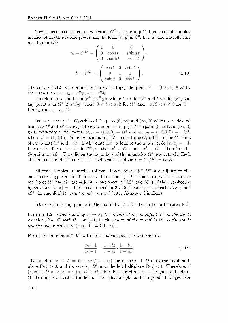
Now let us consider a complexication GC of the group G. It consists of complexmatrice of the third order preserving the form [x, y] in C3. Let us take the followingmatrices in GC:

γt = eitL0 =

1 0 00 cosh t −i sinh t0 i sinh t cosh t

,

δt = eitL2 =

cos t 0 i sin t0 1 0

i sin t 0 cos t

. (1.13)

The curves (1.12) are obtained when we multiply the point x0 = (0, 0, 1) ∈ X bythese matrices, i. e. yt = x0γt, ωt = x0δt.

Therefore, any point x in Y± is x0γtg, where t > 0 for Y+ and t < 0 for Y−, andany point x in Ω± is x0δtg, where 0 < t < π/2 for Ω+ and −π/2 < t < 0 for Ω−.Here g ranges over G.

Let us return to the G1-orbits of the pairs (0, ∞) and (∞, 0) which were deletedfromD×D′ andD′×D respectively. Under the map (1.3) the pairs (0, ∞) and (∞, 0)go respectively to the points ωπ/2 = (i, 0, 0) = ix1 and ω−π/2 = (−i, 0, 0) = −ix1,where x1 = (1, 0, 0). Therefore, the map (1.3) carries these G1-orbits to the G-orbitsof the points ix1 and −ix1. Both points ±x1 belong to the hyperboloid [x, x] = −1.It consists of two the sheets L±, so that x1 ∈ L+ and −x1 ∈ L−. Therefore theG-orbits are iL±. They lie on the boundary of the manifolds Ω± respectively. Eachof them can be identied with the Lobachevsky plane L = G1/K1 = G/K.

All four complex manifolds (of real dimension 4) Y±, Ω± are adjoint to theone-sheeted hyperboloid X (of real dimension 2). On their turn, each of the twomanifolds Ω+ and Ω− are adjoint to one sheet (to iL+ and iL−) of the two-sheetedhyperboloid [x, x] = −1 (of real dimension 2). Relative to the Lobachevsky planeiL± the manifold Ω± is a complex crown (after AkhiezerGindikin).

Let us assign to any point x in the manifolds Y±, Ω± its third coordinate x3 ∈ C.

Lemma 1.2 Under the map x 7→ x3 the image of the manifold Y± is the wholecomplex plane C with the cut [−1, 1], the image of the manifold Ω± is the wholecomplex plane with cuts (−∞, 1] and [1, ∞).

Proof. For a point x ∈ X C with coordinates z, w, see (1.3), we have

x3 + 1

x3 − 1=

1 + iz

1− iz· 1− iw

1 + iw. (1.14)

The function z 7→ ζ = (1 + iz)/(1 − iz) maps the disk D onto the right half-plane Re ζ > 0, and its exterior D′ onto the left half-plane Re ζ < 0. Therefore, if(z, w) ∈ D × D or (z, w) ∈ D′ × D′, then both fractions in the right-hand side of(1.14) range over either the left or the right half-plane. Their product ranges over

1706

Âåñòíèê ÒÃÓ, ò. 16, âûï. 6, ÷. 2, 2011

the whole plane C with cut (−∞, 0]. If in addition z 6= w, then this product is notequal to 1. Hence x3 ranges over C without [−1, 1].

If (z, w) ∈ D×D′ or (z, w) ∈ D′×D, then both fractions in the right-hand sideof (1.14) range over dierent half-planes. Therefore, their product ranges over thewhole of C with cut [0, ∞), hence x3 ranges over C without (−∞, −1] and [1, ∞).Since we consider Ω±, but not D × D′ and D′ × D, we have to exclude in (1.14)pairs (z, w) for which w = 1/z. But it does not make the image smaller. Indead, ifthe rst fraction in the right-hand side of (1.14) has value reiα, −π/2 < α < π/2,then the second fraction has value −r−1eiα, so that their product is equal to −e2iα.The intersection of the sets of these points over all α is empty.

Let M(y) be a holomorphic function on the manifold Y± and let N(x) be itslimit values at the hyperboloid X :

M(x) = limy→x

M(y), y ∈ Y±, x ∈ X .

We shall assume that y tends to x along the radius, i. e. if y ∈ Y± and x ∈ X havehorospherical coordinates (z, w) and (u, v) respectively, then

z = e−tu, w = e−tv (1.15)

and t→ ±0. These equalities (1.15) give (for γt, see (1.13)):

y = xγt. (1.16)

Lemma 1.3 Let M(y) depend only on y3: M(y) = N(y3). By Lemma 1.2 thefunction N(λ) is analytic on the plane C with cut [−1, 1]. Then one has

M(x) = N(x3 ∓ i0x2).

Proof. Let y and x be connected by (1.15). Then by (1.16) we have

y3 = −i sinh t · x2 + cosh t · x3.

Therefore, y3 = −it · x2 + x3 + o(t), when t→ 0. Hence the lemma.

Now let M(ω) be a holomorphic function on the manifold Ω± and let M(x) beits limit values on the hyperboloid X :

M(x) = limy→x

M(ω).

Here we assume similarly that ω tends to x along the radius, i. e. if ω ∈ Ω± andx ∈ X have horospherical coordinates (z, w) and (u, v) respectively, then

z = e−tu, w = etv (1.17)

and t→ ±0.

1707

Âåñòíèê ÒÃÓ, ò. 16, âûï. 6, ÷. 2, 2011

Lemma 1.4 Let M(ω) depend only on ω3: M(ω) = N(ω3). By Lemma 1.2 thefunction N(λ) is analytic on the plane C with cuts (−∞, −1] and [1, ∞). Then

M(x) = N(x3 ± i0 · x1x3) (1.18)

Proof. By (1.17) and (1.18) we have

ω3 =1 + uv

i(e−tu− etv).

Let us substitute here the expressions of u, v in terms of x, see (1.2). Taking intoaccount the equality x2

1 + 1 = (x3 + ix2)(x3 − ix2), we obtain

ω3 =x3

cosh t− i sinh t · x1

. (1.19)

When t→ 0, it behaves as x3(1 + itx1) up to terms of order t2. Hence the lemma.

It is convenient to represent it using a cone in C4. Let us equip C4 with thebilinear form

[[x, y]] = −x0y0 − x1y1 + x2y2 + x3y3

(we add to vectors x in C3 the coordinate x0). Let C be the cone in C4 dened by[[x, x]] = 0, x 6= 0. Then the complex hyperboloid X C is the section of the cone Cby the hyperplane x0 = 1. Looking at (1.3), consider the set Z of points

ζ =1

2(i(z − w), z + w, i(1− zw), 1 + zw) , (1.20)

where z, w ∈ C. It is the section of the cone C by the hyperplane −ix2 +x3 = 1, i. e.the hyperplane [x, ξ0] = 1, where ξ0 = (0, 0, ,−i, 1). The map ζ 7→ x = ζ/ζ0 mapsZ\z = w in X C, it gives just the horospherical coordinates.

The manifolds (1.11) without the points corresponding to∞, lie in Z: in order toobtain D ×D or D′ ×D′, one has to the inequality [ζ, ζ] > 0 to add the inequalityIm (ζ3/ζ2) < 0 or Im (ζ3/ζ2) > 0, respectively, and in order to obtain D × D′ orD′×D, one has to the inequality [ζ, ζ] < 0 to add the condition that the imaginarypart of the determinant ∣∣∣∣ ζ0 ζ1

ζ0 ζ1

∣∣∣∣is less or greater than zero.

[The denition just given of the manifold D ×D is the denition of the Cartandomain of type IV D(p) for p = 2. Indeed, D(p) is dened as follows: we equipCn, n = p + 2, with the form [x, x] = −x2

1 − . . . − x2p + x2

n−1 + x2n. Let ξ

0 =(0, . . . , 0,−i, 1). Then D(p) consists of points ζ ∈ Cn such that

[ζ, ζ] = 0, [ζ, ζ] > 0, [ζ, ξ0] = 1, Im (ζn/ζn−1) < 0.

1708

Âåñòíèê ÒÃÓ, ò. 16, âûï. 6, ÷. 2, 2011

Any point ζ ∈ D(p) can be written as

ζ = (ζ1, . . . , ζp,a− 1

2i,a+ 1

2), a = ζ2

1 + . . .+ ζ2p ,

where ζ1, . . . , ζp satisfy the inequalities:

ζ1ζ1 + . . . ζpζp <aa+ 1

2< 1,

so that D(p) can be identied with a bounded domain in Cp.]

Let us assign to a point x = (x0, x1, x2, x3) in C4 the matrix

x =

(x0 + ix1 x2 + ix3

x2 − ix3 x0 − ix1

). (1.21)

Its determinant is equal to −[[x, x]]. In particular, for a point ζ ∈ Z, given by(1.20), one gets the matrix

ζ = i

(z 1−zw −w

)= i

(1−w

)(z 1

).

These matrices ζ are characterized by det ζ = 0, ζ12 = i.The group G1×G1 acts on the space of matrices (1.21): to an element (g1, g2) ∈

G1 ×G1 corresponds the linear transformation:

x 7→ g−11 xg2. (1.22)

It is given by a real matrix of order 4. We obtain a homomorphism of the groupG1 × G1 onto the group SO0(2, 2). The kernel is the group of order 2 consisting ofthe pairs (E, E), (−E, −E). The diagonal of G1 × G1, i. e. the set of pairs (g, g),g ∈ G1, goes to the subgroup SO0(1, 2) = G, it preserves x0 = (1/2) trx.

Consider the following action of G1 ×G1 on Z:

ζ 7→ g−11 ζg2

−i(g−11 ζg2)12

(apply rst the linear action (1.22) and return then to the section Z along a linepassing through the origin). This is the fractional linear action:

z 7→ z · g2, w 7→ w · g1.

The homomorphism G1 ×G1 → SO0(2, 2) can be extended to the complexications(we obtain a homomorphism SL(2,C) × SL(2,C) → SO(4,C)). Let us take in thecomplexication GC

1 ×GC1 the pairs(

eitL0 , eitL0)and

(e−itL0 , eitL0

).

1709

Âåñòíèê ÒÃÓ, ò. 16, âûï. 6, ÷. 2, 2011

Under the above homomorphism these pairs go to the matrices:1 0 0 00 1 0 00 0 cosh t −i sinh t0 0 i sinh t cosh t

and

cosh t i sinh t 0 0i sinh t cosh t 0 0

0 0 1 00 0 0 1

.

The rst one is obtained by bordering of the matrix γt, see (1.13). The secondone appears in the proof of Lemma 1.4. Indeed, let us multiply a vector (row)(1, x1, x2, x3) in C, such that the vector x = (x1, x2, x3) belongs to X , by this matrixand then divide by the coordinate with index zero, we just get a vector ω ∈ Ω±

whose horospherical coordinates are connected with the horospherical coordinatesof x by (1.17), namely,

ω =1

cosh t− ix1 · i sinh t(x1 · cosh t+ i sinh t, x2, x3) . (1.23)

It includes (1.19). The curve (1.23) with x = x0, i. e. the curve (i tanh t, 0, 1/cosh t),is in fact the curve ωt, see (1.12), with another parameter.

2. On the analytic continuation of spherical functions

First we consider spherical functions Ψσ,ε(x), σ = −1/2 + iρ, ε = 0, 1, on thehyperboloid X of the continuous series. We study the analytic continuation of thesefunctions to the complex manifolds Ω±, dened in 1.

In fact, we may consider the spherical functions Ψσ,ε on the hyperboloid X withgeneric σ: σ ∈ C, σ /∈ Z, not only with σ = −1/2 + iρ.

These spherical functions Ψσ,ε(x), σ ∈ C, ε = 0, 1, were computed in [4], [5], theyare linear combinations of Legendre functions of the rst kind of ±x3 (x3 being thethird coordinate of x):

Ψσ,ε(x) = − 2π

sinσπ[Pσ(−x3) + (−1)εPσ(x3)] . (2.1)

The Legendre function Pσ(z) is analytic in the complex plane C with cut (−∞, −1].At this cut, we dene it as half the sum of the limit values form above and below:

Pσ(c) =1

2[Pσ(c+ i0) + Pσ(c− i0)] , c < −1.

Therefore, the combination Pσ(−z)+(−1)εPσ(z) is analytic in C with cuts (−∞, −1]and [1, ∞). Precisely these cuts appear in Lemmas 1.2 and 1.4 in treating thecomplex manifolds Ω± adjoint to X .

1710

Âåñòíèê ÒÃÓ, ò. 16, âûï. 6, ÷. 2, 2011

So, if we want to continue the functions Ψσ,ε(x) analytically, then naturally Ω±

should be taken for that purpose. Hence let us consider functions on Ω± dened bythe same formula (2.1) with x replaced with ω:

Ψσ,ε(ω) = − 2π

sinσπ[Pσ(−ω3) + (−1)εPσ(ω3)] . (2.2)

These functions are analytic on Ω±. Let us determine their limit values at X .

First consider the function Pσ(ω3) on Ω±. By Lemma 1.4 its limit values at Xare:

limPσ(ω3) =

Pσ(x3), x3 > −1,

Pσ(x3 ∓ i0x1), x3 < −1,(2.3)

when ω → x and ω ∈ Ω±. It follows from [1] 3.3 (10) that the function Pσ(z) hasthe following limit values at the cut (−∞, −1]:

Pσ(c± i0) = e±iσπPσ(−c)− 2

πsinσπ ·Qσ(−c),

where c < −1 and Qσ is the Legendre function of the second kind. Therefore, by(2.3) we have for ω → x, ω ∈ Ω± and x3 < −1:

limPσ(ω3) =

e∓iσπPσ(−x3)− 2

πsinσπQσ(−x3), x1 > 0,

e±iσπPσ(−x3)− 2

πsinσπQσ(−x3), x1 < 0.

It can be written as

limPσ(ω3) = Pσ(c)∓ sgnx1 · isinσπ · Pσ(−x3).

We see that the limit values of Pσ(ω3) as ω → x coincide with Pσ(x3) for x3 > −1only. In order to obtain Pσ(x3) one has to take half the sum of the limit values fromboth manifolds Ω+ and Ω−.

Similarly this goes for Pσ(−y3).

Thus, the limit values at X of the function Ψσ,ε(ω) on Ω± dened by (2.2)coincide with the spherical function Ψσ,ε(x) for −1 < x3 < 1 only. The sphericalfunction Ψσ,ε(x) is even in x1, but the limit function lim Ψσ,ε(ω) does not. In orderto obtain the spherical function Ψσ(x) from the function Ψσ,ε(ω), one has to useboth manifolds Ω± and to take half the sum of the limit values from Ω+ and Ω−:

Ψσ,ε(x) =1

2

∑±

lim Ψσ,ε(ω),

where the limit is taken when ω → x, ω ∈ Ω±, x ∈ X .

1711

Âåñòíèê ÒÃÓ, ò. 16, âûï. 6, ÷. 2, 2011

Now we consider the spherical functions Ψn,± of the holomorphic and anti-holomorphic discrete series on X . Here n ∈ N = 0, 1, 2, . . .. The signs “+′′ and “−′′correspond to the holomorphic and the anti-holomorphic series respectively. Thesefunctions are expressed [4] in terms of Legendre functions of the second kind:

Ψn,±(x) = 4Qn(x3 ∓ i0 · x2).

Comparing it with Lemma 1.3, we see that the spherical function Ψn,± is continuedanalytically on the manifold Y± as the function

Ψn(y) = 4Qn(y3).

References

1. A. Erdelyi, W. Magnus, F. Oberthettinger and F. G. Tricomi. Higher Transcen-dental Functions, McGraw-Hill, New York, 1953.

2. V. F. Molchanov. Quantization on the imaginary Lobachevsky plane, Funct.Anal. Appl., 1980, vol. 14, issue 2, 7374.

3. V. F. Molchanov. Holomorphic discrete series for hyperboloids of Hermitiantype. J. Funct. Anal., 1997, vol. 147, No. 1, 2650

4. V. F. Molchanov. Canonical representations on a hyperboloid of one sheet.Preprint Math. Inst. University of Leiden, MI 2004-02, 56 p.

5. V. F. Molchanov. Canonical and boundary representations on a hyperboloidof one sheet. Acta Appl. Math., 2004, vol. 81, Nos. 13, 191204.

1712