analytic approximations for multi-asset option … · analytic approximations for multi-asset...

Mathematical Finance, Vol. 22, No. 4 (October 2012), 667–689

ANALYTIC APPROXIMATIONS FOR MULTI-ASSET OPTION PRICING

CAROL ALEXANDER AND AANAND VENKATRAMANAN

Reading University

We derive general analytic approximations for pricing European basket and rainbowoptions on N assets. The key idea is to express the option’s price as a sum of prices ofvarious compound exchange options, each with different pairs of subordinate multi-or single-asset options. The underlying asset prices are assumed to follow lognormalprocesses, although our results can be extended to certain other price processes forthe underlying. For some multi-asset options a strong condition holds, whereby eachcompound exchange option is equivalent to a standard single-asset option under amodified measure, and in such cases an almost exact analytic price exists. More gen-erally, approximate analytic prices for multi-asset options are derived using a weaklognormality condition, where the approximation stems from making constant volatil-ity assumptions on the price processes that drive the prices of the subordinate basketoptions. The analytic formulae for multi-asset option prices, and their Greeks, are de-fined in a recursive framework. For instance, the option delta is defined in terms of thedelta relative to subordinate multi-asset options, and the deltas of these subordinateoptions with respect to the underlying assets. Simulations test the accuracy of ourapproximations, given some assumed values for the asset volatilities and correlations.Finally, a calibration algorithm is proposed and illustrated.

KEY WORDS: basket options, rainbow options, best-of and worst-of options, compound exchangeoptions, analytic approximation.

1. INTRODUCTION

This paper presents a recursive procedure for pricing European basket and rainbow op-tions on N assets. The pay-off to a basket option at its maturity T is ω[�NS′

T − K ]+, andthat of a rainbow option is ω[max{S1T , . . . , SNT}− K]+, where ST = (S1T, S2T, . . . , SNT)are the N asset prices, K is the option strike, ω = 1 (call) or −1 (put) and the weights�N = (θ1, θ2, . . . , θN) are real constants. Zero-strike rainbow options are commonlytermed best-of-N-assets or worst-of-N-assets options. Since min {S1T , . . . , SNT} =−max{− S1T , . . . , −SNT}, a pricing model for best-of options also serves for worst-of options. The most commonly traded two-asset options are exchange options (rainbowoptions with zero strike) and spread options (basket options with weights 1 and −1).Margrabe (1978) derived an exact solution for the price of an exchange option, underthe assumption that the two asset prices follow correlated lognormal processes. However,a straightforward generalization of this formula to any two-asset option with non-zerostrike is impossible. A linear combination of lognormal processes is no longer lognormal,and it is only when the strike of a two-asset option is zero that one may circumvent thisproblem by reducing the dimension of the correlated lognormal processes to one. Hence,

Manuscript received July 2009; final revision received September 2010.Address correspondence to Aanand Venkatramanan, ICMA Centre, Henley Business School at Reading,

Reading University, RG6 6BA, UK; e-mail: [email protected].

DOI: 10.1111/j.1467-9965.2011.00481.xC© 2011 Wiley Periodicals, Inc.

667

668 C. ALEXANDER AND A. VENKATRAMANAN

academic research has focussed on deriving good analytic approximations for pricingtwo-asset options with non-zero strike, as well as more general multi-asset options.

Analytic approximations for pricing rainbow options include that of Johnson (1987),who extends the two-asset rainbow option pricing formula of Stulz (1982) to the generalcase of N assets. Ouwehand and West (2006) verify the results of Johnson (1987) andexplain how to prove them using a multivariate normal density approximation derivedby West (2005). Then, they explain how to price N asset rainbow options using thisapproach, providing an explicit approximation for the case N = 4. For options on twoassets with different pay-off profiles, Topper (2001) uses a finite element scheme to solvenonlinear parabolic price PDEs.

Approximations for basket options began with Levy (1992), who approximated abasket price distribution with that of a single lognormal variable, matching the first andsecond moments. Then Gentle (1993) derived the basket option price by approximatingthe arithmetic average by a geometric average. Milevsky and Posner (1998a) used thereciprocal gamma distribution and Milevsky and Posner (1998b) used the Johnson (1949)family of distributions to approximate the distribution of the basket price. Extending theAsian option pricing approach of Rogers and Shi (1995), Beißer (1999) expressed abasket option price as a weighted sum of single-asset Black-Scholes prices, with adjustedforward price and adjusted strike for every constituent asset. Finally, Ju (2002) used aTaylor expansion to approximate the ratio of the characteristic function of the average ofcorrelated lognormal variables, which is approximately lognormal for short maturities.Krekel et al. (2004) compare the performance of these models, concluding that theapproximations of Ju (2002) and Beißer (1999) are most accurate, although they tend toslightly over- and underprice, respectively. However, many of these methods have limitedvalidity or scope. They may require a basket value that is always positive, or they may notidentify the effect of each individual volatility or pair-wise correlation on the multi-assetoption price or its hedge ratios.

This paper develops an analytic approximation that has none of these limitations. Itis based on the novel idea of writing a basket or rainbow pay-off as a sum of pay-offsto compound exchange options (CEOs), where the “assets” in these exchange optionsare pairs of subordinate basket options, and then applying a recursive procedure toobtain a decomposition of the multi-asset option’s pay-off into a sum of pay-offs tostandard, single-asset European calls and puts (henceforth, vanilla options) and optionsto exchange vanilla options on the assets. Each asset price is assumed to follow a standardgeometric Brownian motion (GBM) process, but this assumption may be relaxed to allowmore general drift and local volatility components. The price of a vanilla option followsan Ito’s process, which we approximate with a lognormal process and hence the pricesof the exchange options on vanilla options are obtained using the formula of Margrabe(1978). Then an analytic approximation to the multi-asset option price is given by arecursive application.

In the following, Section 2 presents these recursive pay-off decompositions and de-rives the prices of European basket and rainbow options as linear combinations of pricesof vanilla options and options to exchange such options. Section 3 analyzes CEOs onvanilla options, deriving conditions under which (1) the price processes for the vanillaoptions are approximately lognormal, and (2) their relative prices are almost exactlylognormal. Section 4 derives approximate basket option prices based on both theseconditions. Section 5 presents simulations that illustrate the accuracy of our approxima-tions and Section 6 describes a general calibration algorithm. Section 7 summarizes andconcludes.

ANALYTIC APPROXIMATIONS FOR MULTI-ASSET OPTION PRICING 669

2. PRICING FRAMEWORK

The pay-off to a basket option on N assets with maturity T and (any real) strike K is

VNT = [ω(BT − K)]+ = [ω(�N S′T − K)]+ = [ω�N(S′

T − K′)]+,(2.1)

where BT = �NS′T and K = (K1, K2, . . . , KN) such that �NK′ = K , other notation being

previously defined. Now set �N = (�m, �n), ST = (SmT, SnT), and K = (Km, Kn) forsome positive integers m and n such that m + n = N. Define the sub-basket call and putpay-offs CmT = [�m(S′

mT − K′m)]+, and PmT = [−�m(S′

mT − K′m)]+, and similarly for n.

Then (2.1) becomes

VNT = [CmT − PnT]+ + [CnT − PmT]+.(2.2)

Alternatively, setting �N = (�m, −�n),

VNT = [CmT − CnT]+ + [PnT − PmT]+.(2.3)

The above representations follow on noting that, if f + = max{f , 0} and f − = max{−f ,0} and f and g are any real-valued functions, then [ f + g]+ = [ f + − g−]+ + [g+ − f −]+

and [ f − g]+ = [ f + − g+]+ + [g+ − f +]+. For 0 ≤ t < T , VNt may now be computedas the discounted sum of the risk-neutral expectations of the two replicating CEO pay-offs which appear on the right-hand side: in case (2.2), they are pay-offs to exchangeoptions on a basket call and a basket put; and in case (2.3) they are pay-offs to exchangeoptions on two basket calls and two basket puts with a different number of assets in eachbasket.

Decompositions of the form (2.2) or (2.3) are then applied to each of CmT , PmT , CnT ,and PnT in turn, choosing suitable partitions for m and n which determine the number ofassets in the subordinate basket calls and puts. By applying the pay-off decompositionrepeatedly, each time decreasing the number of assets in the subordinate options, oneeventually expresses the pay-off to an N-asset basket option as a sum of pay-offs to CEOsin which the subordinate options are standard single-asset calls and puts, and ordinaryexchange options. The price of the original N-asset basket option is then computed asthe sum of the prices of CEOs and standard exchange options. We explain how to priceCEOs in terms of standard single-asset option prices in the next section.

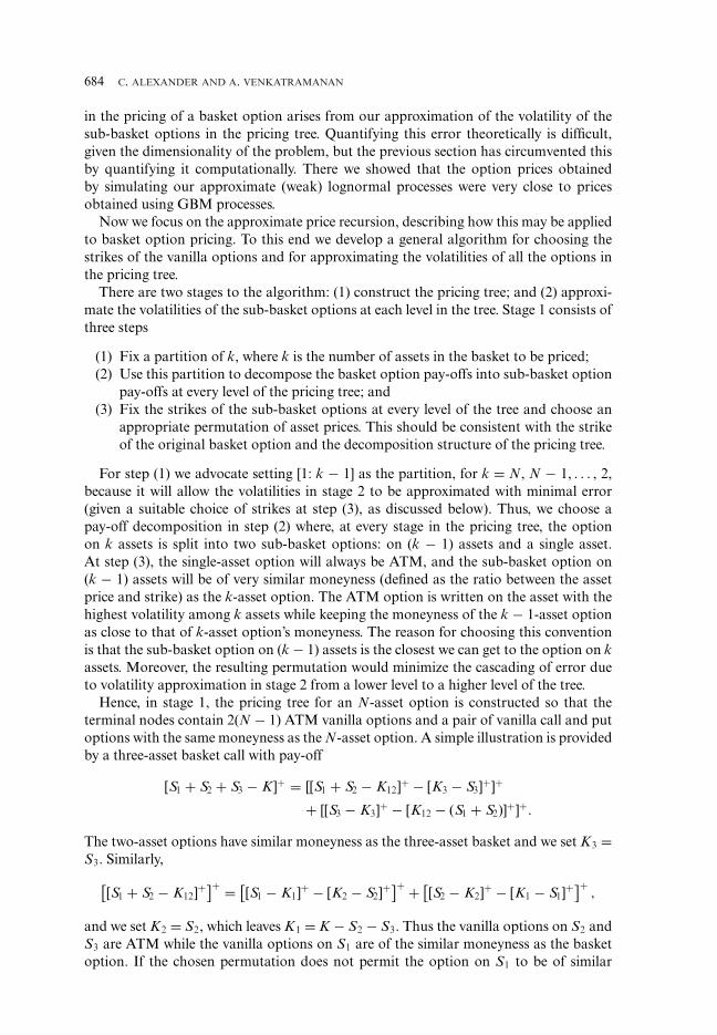
Figure 2.1illustrates this recursive decomposition for pricing a four-asset basket option(we have only shown one leg of the tree, but the other leg can be priced similarly). The four-asset basket option has price equal to the sum of the two CEO prices on the penultimatelevel of the tree. To price these CEOs we have first to compute the prices of the 4 two-assetbasket options on the level below, but to price these we must first price eight CEOs—andto price the CEOs we need to price the standard calls on the four assets (we only needcall prices, because we can deduce the corresponding put prices using put-call parity).

For a general N-asset basket option our approach requires the evaluation of 2(N − 1)CEO prices and 2N standard option prices. When N is odd, terminal nodes will containvanilla options. For instance, for N = 3 and the pay-off [S1T − S2T + S3T − K]+, thedecomposition may be written [[S1T − S2T ]+ − [K − S3T ]+]+ + [[S3T − K]+ − [S2T −S1T ]+]+, so we choose a pair of exchange options on assets one and two and a pair ofvanilla options on asset three. The weighted sum of the strikes of the exchange or vanillaoptions that appear in the terminal nodes of the tree is equal to K, the strike of the basketoption.


FIGURE 2.1. Pricing tree for four-asset basket option.

Now consider a general rainbow option with pay-off max{S1T − K, . . . , SNT − K}. Itsprice may be expressed in terms of an N-asset basket option price and exchange optionprices. To see this, let (n1, n2, . . . , nN) be a permutation of (1, 2, . . . , N) and choose k to besome integer between 1 and N. By splitting the basket of N assets into two sub-baskets,where k determines the size of the sub-baskets and the permutation (n1, n2, . . . , nN)determines the assets in these sub-baskets, the rainbow option’s pay-off may be writtenas the sum of two pay-offs, one to a best-of option on a sub-basket and the other to acompound option, as

max{

Snk+1T, Snk+2T, . . . , SnNT} − K

+ [max

{Sn1T, Sn2T, . . . , SnkT

} − max{

Snk+1T, Snk+2T, . . . , SnNT}]+

.

The best-of option pay-off terms here may themselves be represented as the sum of twosuch pay-offs, until all sub-baskets are on one or two assets. Once the sub-basket size iseventually reduced to two, we use the identity max{SiT , SjT} = SjT + [SiT − SjT ]+.

For every permutation (n1, n2, . . . , nN) and index k we obtain a different pay-offdecomposition for the rainbow option. Obviously, the value of the pay-off will be thesame in each case, so the model should be calibrated in such a way that the option priceis invariant to the choice of (n1, n2, . . . , nN) and k. For illustration, consider a rainbowoption on four assets. Here, it is convenient to use the notation Xni t for the price of anoption to receive asset ni in exchange for selling asset ni+1. Choosing (n1, n2, n3, n4) = (1,2, 3, 4) and k = 2, the rainbow option’s pay-off P4T may be written P4T = S4T + X3T +[BT ]+ − K. Thus, the price of the rainbow option is P4t = S4t + X3t + Vt − Ke−r(T−t),where Vt = e−r (T−t)EQ{[BT]+} is the price of a zero-strike basket option with four assetswhose prices are {X1t, S2t, X3t, S4t} and with weights {1, 1, −1, −1}. Recall that, underthe correlated lognormal assumption, an analytic solution exists for Xit. Hence, P4t maybe evaluated because we have already derived the price Vt of the basket option; it may beexpressed in terms of CEO prices.

We have chosen k = 2 above because this choice leads to the simplest form of pay-offdecomposition for a four-asset rainbow option. In fact, for any permutation (n1, n2, n3,n4), the pay-off may be written P4T = Sn4T + Xn3T + [Sn2T − Xn1T − Sn4T + Xn3T]+ − K .Hence, a general expression for the price of a four-asset rainbow option is P4t = Sn4t +Xn3t + V4t − Ke−r (T−t), where V4t = e−r (T−t)EQ{[BT]+} denotes the price of a zero-strike


basket option with four assets whose prices are {Xn1t, Sn2t, Xn3t, Sn4t} and with weights{1, 1, −1, −1}. This argument can be extended to rainbow options on more than fourassets. For example, the pay-off to a rainbow option on three assets, having prices S5,S6, and S7, may be written P3T = S7T + X6T + [S5T − S7T + X6T ]+, and the price of aseven-asset rainbow option is P7t = P3t + EQ{[P4T − P3T]+}.

3. PRICING CEO’S

The pay-off decompositions illustrated above have employed options on a basket whichmay contain the assets themselves, options written on these assets, and options to ex-change these assets. A suitable pay-off decomposition will express the price of thesebasket options as a sum of CEO prices. The two options exchanged in the CEO (whichmay be on different assets or may themselves be compound options) always have the samematurity as the CEO. We now derive an analytic approximation for the CEO price, firstassuming the underlying assets follow correlated lognormal processes, and then undermore general price processes. Our key idea is to express the price of such a CEO as theprice of a single-asset option that can be easily derived.

Let (�, (Ft)t≥0, Q) be a filtered probability space, where � is the set of all possibleevents such that S1t, S2t ∈ (0, ∞), (Ft)t≥0 is the filtration produced by the sigma algebraof the price pair (S1t, S2t)t�0 and Q is a bivariate risk-neutral probability measure.Assume the risk-neutral price dynamics are governed by dSit = rSitdt + σ iSitdWit with〈dW 1t, dW 2t〉 = ρdt for i = 1, 2, where W 1 and W 2 are Wiener processes under therisk-neutral measure Q, σ i is the constant volatility of asset i, and ρ is the constantcorrelation between dW 1 and dW 2. Consider an option to exchange a vanilla option onasset one with a vanilla option on asset two, where all options have the same maturityT . Let Uit and Vit denote the prices of the vanilla call and put on asset i with commonstrike Ki, for i = 1, 2. If the CEO is on two calls the pay-off is [ω(U1T − U2T )]+, if theCEO is on two puts the pay-off is [ω(V1T − V2T )]+, and the pay-off is either [ω(U1T −V2T )]+ or [ω(V1T − U2T )]+ if the CEO is on a call and a put, where ω = 1 for a call CEOand −1 for a put CEO.

The price ft of a CEO can be obtained as a risk-neutral expectation of the terminalpay-off, for example, for a CEO on two calls

ft = e−r (T−t)EQ{[ω(U1T − U2T)]+|Ft}.

But the application of risk-neutral valuation requires a description of the price processesUit and Vit, for i = 1, 2. To this end we apply Ito’s Lemma to ft and use the Black-Scholesdifferential equation to obtain

dUit =(

∂Uit

∂t+ r Sit

∂Uit

∂Sit+ 1

2σ 2

i S2it∂2Uit

∂S2it

)dt + σi Sit

∂Uit

∂SitdW it

= rUit dt + ξitUit dW it,

(3.1)

where ξit = σiSitUit

∂Uit∂Sit

. Similarly, setting ηit = σiSitVit

| ∂Vit∂Sit

| yields

dVit = r Vit dt + ηitVit dW it.(3.2)

We restrict our subsequent analysis to pricing a CEO on two calls (the followingderivations are very similar when one or both of the standard options are puts). We first


solve for the prices Uit of the underlying options and their volatilities ξ it, for i = 1, 2.Then we derive “weak” and “strong” lognormality conditions, under which the CEOprice is approximately equal to a single-asset option price under an equivalent measure.

LEMMA 3.1. When the asset price Sit follows a GBM with Wiener process Wit, a standardcall option on asset i has price process described by (3.1) with volatility ξ it following theprocess described by

dξit = ξit

(σi − ξit + σi Sit

it

�it

)[−ξit dt + dW it] ,(3.3)

where �it = ∂Uit∂Sit

and it = ∂�it∂Sit

are the delta and gamma of the call option.

Proof . Let θit = ∂Uit∂t and Xit = �it

Uit. Then, dropping the subscripts, dξ = σ (XdS +

SdX + dSdX). By Ito’s Lemma

d� = ∂θ

∂Sdt + ∂�

∂S(r Sdt + σ SdW) + 1

2∂2�

∂S2σ 2S2 dt

= ∂

∂S(rU) dt − (r� + σ 2S) dt + σ SdW

= −σ 2Sdt + σ SdW,

and

d X = U−1 d� − U−2�dU + U−3�dU2 − U−2d�dU

= U−1 (�ξ 2 − σ Sξ − r� − σ 2S

)dt + U−1 (σ S − ξ�) dW.

Hence dξ = (σξ − ξ 2 + σ 2 S2

U ) [−ξdt + dW], which can be rewritten as (3.3). �The only approximation we need to make is that σ iSitit/�it is constant in equa-

tion (3.3), that is, set ci = σ iSitit/�it and write σi = σi + ci . Then (3.3) becomes

dξit = ξit(ξit − σi ) (ξit dt − dW it) .(3.4)

LEMMA 3.2. Let ki = σi/ξ0 − 1 and W∗it = − 1

2 σ t + Wit, for i = 1, 2. Then (3.4) hassolution

ξit = σi (1 + ki e−σi W∗it )−1.(3.5)

For ξ it to remain finite, we must have W∗it > 1

2 σi t + σ−1i ln |ki | for all t ∈ [0, T ]. When

ξi0 > σi the option volatility process explodes in finite time and the boundary at ∞ is anexit boundary.

Proof . The proof is the same for i = 1 and 2, so we can drop the subscript i forconvenience. If ξ0 = σ then ξt = σ for all t > 0. So in the following we consider twoseparate cases, according as ξ0 < σ and ξ0 > σ .

It follows from (3.4) that dξ t → 0 whenever ξ t → 0 or σ . So if the process is startedwith a value ξ0 < σ then ξ t will remain bounded between 0 and σ (σ ≥ ξt ≥ 0) for all t∈ [0, T ]. On the other hand, when ξ0 > σ , ξ t is bounded below by σ but not bounded


above, and ξt − σ ≥ 0. Setting xt = 1σ

ln | ξt−σ

ξt| and applying Ito’s Lemma, we can show

that dxt = 12 σdt − dW t and xt = x0 + 1

2 σ t − Wt. Substituting xt back into the aboveequation yields ξt = σ (1 + ke−σ W∗

t )−1.Now we show that the option volatility process explodes when ξi0 > σi and the bound-

ary at ∞ is an exit boundary. That is, ξ it reaches ∞ in finite time and once it reaches ∞,it stays there. From the above equation, we see that ξ t → ∞ when W∗

t → σ−1 ln |k|. Sothe volatility process could reach ∞ in finite time. However, when W∗

t < σ−1 ln |k| theabove equation implies that ξ t could become negative, which cannot be true. So to provethat ξ t remains strictly positive, we need to know more about the boundary at ∞. If theboundary is an “exit” boundary, then ξ t cannot return back once it enters the region.That is, if ξ τ = ∞ for some stopping time 0 ≤ τ ≤ T , then ξ s = ∞ for all s > τ .

In fact, we can indeed classify ∞ as an exit boundary, and to show this we perform thetest described in Lewis (2000), Durrett (1996), and Karlin and Taylor (1981). To this end,let s(y), m(y) be functions such that, for 0 < y < ∞, s(y) = exp{− ∫ y 2α(x)

β(x)2 dx}, m(y) =β(y)2s(y). Define S(c, d), M(c, d), and N(d) as S(c, d) = ∫ d

c s(y) dy, M(c, d) = ∫ dc

1m(y) dy,

N(d) = limc↓0∫ d

cS(c,y)m(y) dy. Then, the Feller test states that the boundary at ∞ is an

exit boundary of the process if M(0, d) = ∞ and N(0) < ∞. In our case, we haveα(x) = x2(x − σ ) and β(x) = −x(x − σ ), so

m(y) = σ 2 y2; s(y) = exp{−

∫ y 2x − σ

dx}

= σ 2

(y − σ )2

M(c, d) = 1σ 2

[1c

− 1d

]; S(c, d) = σ 2

[1

σ − d− 1

σ − c

]

N(d) =∫ d

0S(0, x)m(x) dx = − d

σ− ln |d − σ | + ln σ .

This shows that M(0, d) = ∞ and N(0) < ∞, hence ξ it explodes and ∞ is an exitboundary. �

Now that we have characterized the option price volatility, it is straightforward to findthe option price under our lognormal approximation, as follows:

LEMMA 3.3. When the option volatilities are given by (3.5) the call option price at timet is

Uit = Ui0 ert

(eσi W∗

it + ki)

1 + ki,(3.6)

where ki = ( σiξi0

− 1) and W∗it = − 1

2 σ t + Wit. Moreover, when ξi0 > σi , Uit → 0 as ξ it →∞.

Proof . Given the option price SDE (3.1), dropping the subscript i and solving for U ,we get

Ut = U0 exp(

rt − 12

∫ t

0ξ 2

t dt +∫ t

0ξt dW t

).(3.7)

Substituting d(ln |σ − ξt|) = 12ξ 2

t dt − ξt dW t in the above equation gives


Ut = U0 exp(

rt −∫ t

0d(ln |σ − ξt|)

)

= U0 exp(rt − ln |σ − ξt| + ln |σ − ξ0|)

= U0ert(

σ − ξ0

σ − ξt

),

(3.8)

which can be rewritten as equation (3.6). �From Lemma 3.3, since ξ t is bounded between 0 and σ when ξ0 < σ and bounded

below by σ when ξ0 > σ , we can conclude that Ut will remain strictly positive for all timet ∈ [0, T ]. However, for ξ0 > σ , if the volatility explodes (ξ t → ∞), equation (3.8) showsthat Ut → 0. Moreover, once Ut reaches zero, it will stay there.

The option price process (3.6) will follow an approximately lognormal process ifξi0 ≈ σi , and we call this the weak lognormality condition. But when is ξi0 ≈ σi ? Bydefinition, ξit → σ i if ∂Uit

∂Sit→ 1 and Sit

Uit→ 1 as t → T . Then, σ i ≈ σi and therefore

ξi0 ≈ σi . Moreover, from equation (3.5), ξit ≈ σi , for all t ∈ [0, T ]. Under the weaklognormality condition, the option price volatilities ξ it and ηit are directly approximatedas constants in equations (3.1) and (3.2), respectively. This allows us to approximate theoption price processes as lognormal processes. Hence, we can change the numeraire tobe one of the option prices, so that the price of a CEO may be expressed as the price ofa single-asset option, and we can price the CEO using the formula given by Margrabe(1978).

The weak lognormality condition is used to derive analytic approximations to basketoption prices in Section 4. However, for some multi-asset options it is possible to obtainan almost exact price. The following result provides a strong lognormality condition,under which the relative option price follows a lognormal process almost exactly.

THEOREM 3.4. The CEO on calls has the same price as a standard single-asset optionunder a modified yet equivalent measure if the following condition holds

U10k1

1 + k1− U20

k2

1 + k2= 0.(3.9)

Proof . The call CEO on two calls has time 0 price given by

f0 = e−r TEQ

{[U10er T

1 + k1

(eσ1W∗

1T − k1) − U20er T

1 + k2

(eσ2W∗

2T − k2)]+}

= EQ

{[U10

1 + k1eσ1W∗

1T − U20

1 + k2eσ2W∗

2T −(

U10k1

1 + k1− U20

k2

1 + k2

)]+}

= EQ

{[U10

1 + k1exp

(∫ T

0−1

2σ 2

1 ds + σ1 dW 1s

)

− U20

1 + k2exp

(∫ T

0−1

2σ 2

2 ds + σ2 dW 2s

)]+}.

(3.10)


Let dW 1t = ρdW 2t + ρ ′dZ1t, where W 2 and Z1 are independent Wiener processes,ρ ′ =

√1 − ρ2 and P is a probability measure whose Radon-Nikodym derivative with

respect to Q is given by

dP

dQ= exp

(−1

2σ 2

2 t + σ2W2t

).

Let Yt = U1t(1+k2)U2t(1+k1) and Z2t = W2t − σ2t. Then Z1 and Z2 are independent Brownian mo-

tions under the measure P and the dynamics of Y can be described by

d(ln Yt) =(

−12σ 2

1 + 12σ 2

2

)dt + (ρσ1 − σ2) dW 2t − ρ ′σ1d Z1t = −1

2σ 2dt + σt dW t,

where W is a Brownian motion under P and σ 2 = (ρσ1 − σ2)2 + (ρ ′σ1)2 = σ 21 + σ 2

2 −2ρσ1σ2. Now the CEO price can be written as the price of a single-asset option writtenon Y , as

f0 = U20

1 + k2EP

{[Yt exp

(−1

2

∫ T

0σ 2

s ds +∫ T

0σs dW s

)− 1

]+}= U20

1 + k2EP{[YT − 1]+}.

When σi > ξi0, for i = 1, 2, the above expectation simply yields the Black-Scholes priceof a European option on Yt with strike equal to one. But when σi < ξi0, ξ iτ could reach∞ for some τ ≤ T . However, when the volatility explodes Uis = 0 for s ≥ τ , since theboundary at ∞ is an exit boundary, and the expectation in equation (3.10) need only becomputed over the paths for which the individual option volatilities remain finite. Nowby Lemma 3.2,

Z1t > ρ ′−1(

12

(σ1 − σ2)t + σ−11 ln |k1| − σ−1

2 ln |k2|)

= μ1

and Z2t > − 12 σ2t + σ−1

2 ln |k2| = μ2.

Hence, setting mi = min {Zis: 0 ≤ s ≤ T}, the price of the CEO may be written

f0 = U20

1 + k2EP{1m1>μ1;m2>μ2 [YT − 1]+} + U10

1 + k1EQ

{1m1>μ1;m2<μ2

[eσ1W∗

1T − k1]+}

,

(3.11)

where 1 is the indicator function. The first term on the right-hand side gives the expectedvalue of the pay-off when neither of the volatilities explode. This is equal to the price of adown-and-out barrier exchange option which expires if either of the asset prices crossesthe barrier. The second term is equivalent to a single-asset external barrier option whenonly ξ 2 explodes. Then U2T becomes zero and the CEO pay-off reduces to U1T .

Single-asset barrier options can be priced by an application of the reflection principle(see Karatzas and Shreve 1991) and the case of a two-asset barrier exchange option is anextension of that.1 Using the reflection principle, the first term in the right-hand side ofequation (3.11) may be written

EP

{1YT>1; m1>μ1; m2>μ2

} = EP

{1YT>1; m1>μ1

} − EP

{1ln YT< 2μ2 ; m1>μ1

}.

1 Carr (1995), Banerjee (2003), and Kwok, Wu, and Yu (1998) discuss the pricing of two-asset and multi-asset external barrier options that knock out if an external process crosses the barrier. Lindset and Persson(2006) discuss the pricing of two-asset barrier exchange options, where the option knocks out if the price ofone asset equals the other.


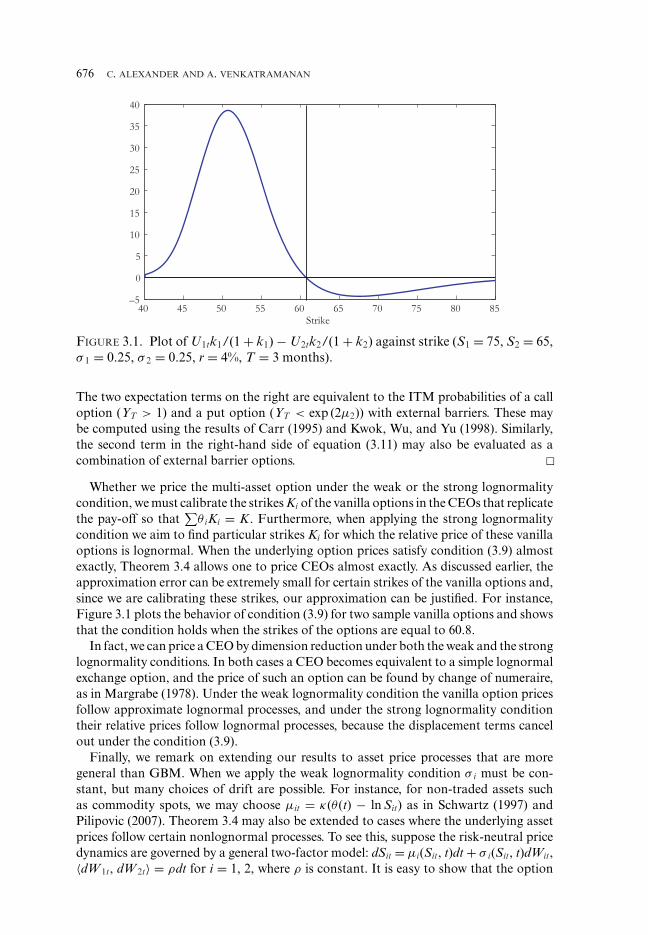
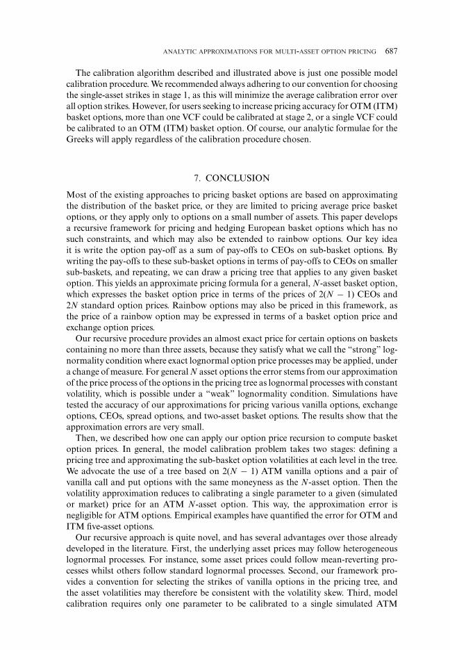
FIGURE 3.1. Plot of U1tk1/(1 + k1) − U2tk2/(1 + k2) against strike (S1 = 75, S2 = 65,σ 1 = 0.25, σ 2 = 0.25, r = 4%, T = 3 months).

The two expectation terms on the right are equivalent to the ITM probabilities of a calloption (YT > 1) and a put option (YT < exp (2μ2)) with external barriers. These maybe computed using the results of Carr (1995) and Kwok, Wu, and Yu (1998). Similarly,the second term in the right-hand side of equation (3.11) may also be evaluated as acombination of external barrier options. �

Whether we price the multi-asset option under the weak or the strong lognormalitycondition, we must calibrate the strikes Ki of the vanilla options in the CEOs that replicatethe pay-off so that

∑θ iKi = K. Furthermore, when applying the strong lognormality

condition we aim to find particular strikes Ki for which the relative price of these vanillaoptions is lognormal. When the underlying option prices satisfy condition (3.9) almostexactly, Theorem 3.4 allows one to price CEOs almost exactly. As discussed earlier, theapproximation error can be extremely small for certain strikes of the vanilla options and,since we are calibrating these strikes, our approximation can be justified. For instance,Figure 3.1 plots the behavior of condition (3.9) for two sample vanilla options and showsthat the condition holds when the strikes of the options are equal to 60.8.

In fact, we can price a CEO by dimension reduction under both the weak and the stronglognormality conditions. In both cases a CEO becomes equivalent to a simple lognormalexchange option, and the price of such an option can be found by change of numeraire,as in Margrabe (1978). Under the weak lognormality condition the vanilla option pricesfollow approximate lognormal processes, and under the strong lognormality conditiontheir relative prices follow lognormal processes, because the displacement terms cancelout under the condition (3.9).

Finally, we remark on extending our results to asset price processes that are moregeneral than GBM. When we apply the weak lognormality condition σ i must be con-stant, but many choices of drift are possible. For instance, for non-traded assets suchas commodity spots, we may choose μit = κ(θ (t) − ln Sit) as in Schwartz (1997) andPilipovic (2007). Theorem 3.4 may also be extended to cases where the underlying assetprices follow certain nonlognormal processes. To see this, suppose the risk-neutral pricedynamics are governed by a general two-factor model: dSit = μi(Sit, t)dt + σ i(Sit, t)dWit,〈dW 1t, dW 2t〉 = ρdt for i = 1, 2, where ρ is constant. It is easy to show that the option


price processes will still be given by (3.6) whenever μi(Sit, t) and σ i(Sit, t) satisfy(∂σit

∂t+ μit

∂σit

∂Sit+ 1

2σ 2

it∂2σit

∂S2it

)= σit

∂μit

∂Sit.

4. PRICING BASKET OPTIONS

First, we apply the strong lognormality condition and use the formula of Margrabe(1978) recursively to derive almost exact prices for specific examples of basket optionswith two or three assets. However, when N ≥ 4 the condition in Theorem 3.4 is toostrong. In that case, we derive analytic approximate basket option prices under the weaklognormality condition.

Consider a CEO written on two lognormal exchange options, both having a commonasset which is used as numeraire in the method of Margrabe (1978). Then the exchangeoption price processes may be described by equations (3.1) or (3.2), and the CEO can bepriced by applying Theorem 3.4. For example, the pay-off to a two-asset basket optioncan be written as a sum of pay-offs to two CEOs on single-asset call and put options,as in Section 3. A three-asset basket option with zero strike, when the signs of the assetweights � are a permutation of (1, 1, −1) or (−1, −1, 1), is just an extension of thetwo-asset case where we have an additional asset instead of the strike. The option canbe priced as a CEO either to exchange a two-asset exchange option for the third assetor to exchange 2 two-asset exchange options with a common asset. For example, a 3:2:1spread option has pay-off decomposition2

PT = [3S1T − 2S2T − S3T]+

= [3[S1T − S2T]+ − [S3T − S2T]+]+ + [[S2T − S3T]+ − 3[S2T − S1T]+]+.

In the general case of basket options on N underlying assets, except for the onesdiscussed above, the two replicating CEOs are no longer written on plain vanilla orlognormal exchange options, but on sub-basket options. For instance, consider a four-asset basket option with zero strike and pay-off PT = [S1T − S2T − S3T + S4T ]+. Wehave

PT = [[S1T − S2T]+ − [S3T − S4T]+]+ + [[S4T − S3T]+ − [S2T − S1T]+]+,

and since the two replicating CEOs are written on lognormal exchange options with nocommon asset, the CEOs cannot be priced using Theorem 3.4. But we can adjust thevolatilities of the CEOs using the weak lognormality condition, so that the sub-basketoption price processes are approximately lognormal processes. Then the relative sub-basket option prices also follow approximate lognormal processes and the two replicatingCEO prices can be computed by using the formula of Margrabe (1978). Thus, exactpricing under the strong lognormality condition is only possible in special cases, and inthe general case we must use the weak lognormality condition to find an approximateprice.

2 Note that there is a closed form formula for the price of this option of the form∫ ∞

−∞

∫ ln 32 +x

−∞

∫ ln(3ex−2ey)

∞(3ex − 2ey − ex) f (x, y, z) dz dy dx,

where f is the trivariate normal density function and x, y, z are the log stock price processes. However, it isnot easy to evaluate the triple integral.


Let(�, (Ft)t≥0 , Q

)be a filtered probability space, where � is the set of all possible

events such that (S1t, S2t, . . . , SNt) ∈ (0, ∞)N , (Ft)t≥0 is the filtration produced by thesigma algebra of the N-tuplet (S1t, S2t, . . . , SNt)t≥0 of asset prices, and Q is a multivariaterisk-neutral probability measure. We assume that the underlying asset prices processesSi are described by

d Sit = μi (Sit, t)Sit dt + σi Sit dW it, 〈 dW it, dW jt〉 = ρi j dt, 1 ≤ i , j ≤ N,

where Wi are Wiener processes under the risk-neutral measure Q, σ i is the volatility ofith asset (assumed constant), μi(.) is a well-defined function of Sit and t, and ρ ij is thecorrelation between ith and jth assets (assumed constant).

We now describe the price process VNt of the basket option on N assets. Using arecursive argument, we begin by assuming that the prices of the call and put sub-basketoptions on m and n assets follow lognormal processes. Then we show that when the basketoption volatility is approximated as a constant the basket option price process VNt canbe expressed as a lognormal process. Since Cmt, Cnt, Pmt, and Pnt are prices of basketoptions themselves, we may also express their processes as lognormal process, assumingtheir sub-basket option prices follow lognormal processes. In the end, these assumptionsyield an approximate lognormal process for the price of a basket option on N assets.

As before, let �N = (�m, −�n). Then the basket option price may be computed as asum of the price E1t of a CEO on two sub-basket calls and the price E2t of a CEO on twosub-basket puts, that is, VNt = E1t + E2t. Each sub-basket option follows a price processwith a nonconstant volatility, but we shall express it using a constant. For instance, thesub-basket call option price processes are written, for i = m and n

dCit = rCit dt + σ Ci Cit dWit,

where Wi is a Wiener process and σ Ci is a constant.3 Then, by Ito’s Lemma

d E1t = r E1t dt +∑

i=m,n

σ Ci Cit�Cit dWit.(4.1)

Similarly, we assume the price E2t of the CEO on puts follows a process analogous to(4.1) with Ci replaced by Pi; and when the decomposition gives two CEOs written oncall and put sub-basket options, so their price processes have a call and a put optioncomponent, we have

d E1t = r E1t dt + σ CmCmt�Cmt dWmt + σ Pn Pnt�Pnt dWnt.

Now write dWnt = γ mn dWmt +√

1 − γ 2mn dWt, where W is a Wiener process, independent

of Wm, and γ mn is the correlation between the options on sub-baskets of size m and n.Further, define

σit = σ Ci

Cit

VNt

∂ E1t

∂Cit− σ Pi

Pit

VNt

∂ E2t

∂ Pit,

for i = m and n.

3 For brevity, we suppress the dependence of σCi on the option’s strike and maturity, the discount rateetc.


Then

dVNt = r (E1t + E2t) dt +∑

i=m,n

σCi Cit�Cit dWit −∑

i=m,n

σPi Pit�Pit dWit,

= r VNt dt + VNt

((σCm

Cmt

VNt

∂ E1t

∂Cmt− σPm

Pmt

VNt

∂ E2t

∂ Pmt

)dWmt

−(

σCnCnt

VNt

∂ E1t

∂Cnt− σPn

Pnt

VNt

∂ Ent

∂ Pnt

)dWnt

),

= r VNt dt + VNt(σmt dWmt − σnt dWnt

).

Now setting

σ 2t = σ 2

mt + σ 2nt − 2γmn σmtσnt,

σ 2E1t = σ 2

Cmt + σ 2Cnt − 2γmn σCmtσCnt,

σ 2E2t = σ 2

Pmt + σ 2Pnt − 2γmn σPmtσPnt

yields

dVNt = r VNt dt + σtVNt dWt.(4.2)

So that its price is given by Margrabe’s formula, the basket option price VNt is approx-imated by a lognormal process, that is, we replace the volatility in the SDE (4.2) by aconstant, σ . Thus, in place of (4.2) we assume dVNt = r VNt dt + σ VNt dWt.

Let ν be a positive real such that σ = ν σ0, where σ0 is the value of σt at time zero.Then dVNt = r VNt dt + ν σ0VNt dWt. We have also assumed that the underlying call andput sub-basket options follow lognormal processes, with average volatilities σCi and σPi ,respectively. Thus, we could likewise set σCi = νCi σCi ,0 and σPi = νPi σPi ,0. However, forease of calibration we shall use only one parameter for the volatilities of all the optionsabove the base level of the pricing tree. That is, we set all ν’s equal to a constant, ν,which we call the “volatility correction factor” (VCF).4 Thus, σ ≈ ν σ0, σCi ≈ ν σCi ,0,σPi ≈ ν σPi ,0, and so on. Note that σE1t is also replaced by a constant σE1, and with asingle VCF ν, σE1 ≈ ν (σ 2

Cm0 + σ 2Cn0 − 2γmn σ Cm0σCn0)1/2 and similarly for σE2.

THEOREM 4.1. The price of a general N-asset basket option may be approximated bythe recursive formula

VNt(�, St, K, T, ν, ω) = E1t(�, St, K, T, ν, ω) + E2t(�, St, K, T, ν, ω),(4.3)

4 The VCF does not apply to single-asset option volatilities. When the sub-basket size reduces to one, ν

= 1 and the option has price process (3.1) if it is a call, or (3.2) if it is a put. The sole function of the VCF isto approximate the process volatilities of the options above the base level of the tree.


where

E1t(�, St, K, T, ν, ω) = ω(Vmt(�m, SmT, Km, ν,+1)�(ωd11)

− Vnt(�n, SnT, Kn, ν,−χ )�(ωd12))

= ω(V1

mt�(ωd11) − V1nt�(ωd12)

), say

E2t(�, St, K, T, ω) = ω(Vnt(�n, SnT, Kn, ν, χ )�(ωd21)

− Vmt(�m, SmT, Km, ν,−1)�(ωd22))

= ω(V2

nt�(ωd21) − V2mt�(ωd22)

), say

with χ = +1 for a call and −1 for a put, and

di1 = ln(Vi

mt

/Vi

nt

) + 12ν2σ 2

Ei (T − t)

νσEi√

T − t; di2 = di1 − νσEi

√T − t.

Proof . Since Cm, Pm and Cn, Pn are themselves prices of options on baskets of sizesm and n, respectively, they can be computed by applying equation (4.3) recursively untilthe size of a sub-basket reaches one and St = (Sit), K1 = (Ki ), and �1 = θi for some 1 ≤i ≤ N. Then

E1(�, St, K, T, 1, ω) =ωe−r (T−t)θi (Fit,T�(ωd1) − Ki�(ωd2)) , E2(�, St, K, T, 1, ω) = 0,

where Fit,T is the ith asset forward price and

d1 =[

ln(FitT/Ki ) +(

r + 12�2

i

)(T − t)

] /[�i

√T − t] , d2 = d1 − �i

√T − t.

For instance, when μi = (r − qi) in equation (4.1), Fit,T = Site(r−qi )(T−t) and �i = σ i. Ormore generally, when μi = κ(θ (t) − ln Sit), as in Pilipovic (2007)

Fit,T = exp(

e−κ(T−t) ln Sit +∫ T

te−κ(T−s)θ (s) ds + σ 2

i

2κ(1 − e−2κ(T−t))

),

�i = σi

√1 − e−2κ(T−t)

2κ.

�One of the main advantages of our approximation is that we can derive analytic

formulae for the multi-asset option Greeks which, unlike most other approximations,capture the effects that individual asset’s volatilities and correlations have on the hedgeratios. Differentiating the basket option price given in Theorem 4.1, using the chain rule,yields the following

COROLLARY 4.2. The deltas, gammas, and vegas of our basket option price f are

�fSi

= �fCj

�Cj

Si+ �

fPj

�Pj

Si

fSi

= f

Cj

(�

Cj

Si

)2 + Cj

Si�

fCj

+ fPj

(�

Pj

Si

)2 + Pj

Si�

fPj

V fσi

= V fσE1

∂σE1

∂σi+ V f

σE2

∂σE2

∂σi+ VCj

σi �fCj

+ V Pjσi �

fPj

,

(4.4)


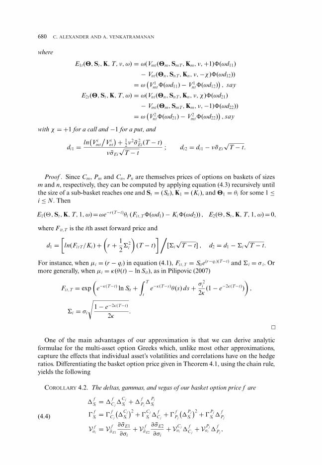
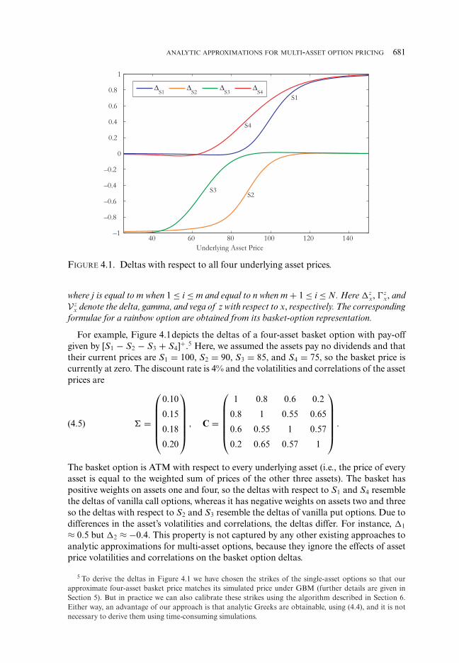
FIGURE 4.1. Deltas with respect to all four underlying asset prices.

where j is equal to m when 1 ≤ i ≤ m and equal to n when m + 1 ≤ i ≤ N. Here �zx, z

x, andV z

x denote the delta, gamma, and vega of z with respect to x, respectively. The correspondingformulae for a rainbow option are obtained from its basket-option representation.

For example, Figure 4.1depicts the deltas of a four-asset basket option with pay-offgiven by [S1 − S2 − S3 + S4]+.5 Here, we assumed the assets pay no dividends and thattheir current prices are S1 = 100, S2 = 90, S3 = 85, and S4 = 75, so the basket price iscurrently at zero. The discount rate is 4% and the volatilities and correlations of the assetprices are

� =

⎛⎜⎜⎜⎜⎜⎝

0.10

0.15

0.18

0.20

⎞⎟⎟⎟⎟⎟⎠ , C =

⎛⎜⎜⎜⎜⎜⎝

1 0.8 0.6 0.2

0.8 1 0.55 0.65

0.6 0.55 1 0.57

0.2 0.65 0.57 1

⎞⎟⎟⎟⎟⎟⎠ .(4.5)

The basket option is ATM with respect to every underlying asset (i.e., the price of everyasset is equal to the weighted sum of prices of the other three assets). The basket haspositive weights on assets one and four, so the deltas with respect to S1 and S4 resemblethe deltas of vanilla call options, whereas it has negative weights on assets two and threeso the deltas with respect to S2 and S3 resemble the deltas of vanilla put options. Due todifferences in the asset’s volatilities and correlations, the deltas differ. For instance, �1

≈ 0.5 but �2 ≈ −0.4. This property is not captured by any other existing approaches toanalytic approximations for multi-asset options, because they ignore the effects of assetprice volatilities and correlations on the basket option deltas.

5 To derive the deltas in Figure 4.1 we have chosen the strikes of the single-asset options so that ourapproximate four-asset basket price matches its simulated price under GBM (further details are given inSection 5). But in practice we can also calibrate these strikes using the algorithm described in Section 6.Either way, an advantage of our approach is that analytic Greeks are obtainable, using (4.4), and it is notnecessary to derive them using time-consuming simulations.


5. SIMULATION RESULTS

This section tests the accuracy of the weak lognormal approximation by comparing thesimulated price of various options based on standard correlated GBM processes withthat based on the approximate process (4.2). We have seen that we price a multi-assetoption as a sum of CEOs on sub-basket options. These sub-basket options are in turnpriced as sums of CEOs of smaller baskets until we arrive at a sum of CEOs on vanillacall and put options. By rewriting the option price processes as approximate lognormalprocesses we are able to apply Margrabe’s formula to compute the price of the CEO,and hence also the price of the multi-asset option. Therefore, the accuracy of our weaklognormal approximation for pricing CEOs is crucial for the accuracy of our multi-assetoption price approximations.

Consider the compound call exchange option that is an option to receive a vanilla callon asset one in exchange for a vanilla call on asset two, which has pay-off

PT = [U1T − U2T]+, with U1t = [S1t − K1]+ and U2t = [S2t − K2]+.

We now simulate the price of this option in two different ways, by: (1) simulating theunderlying asset prices themselves, using correlated GBMs; and (2) simulating the CEOprice Pt directly using our lognormal approximation, viz:

d Pt

Pt= rdt + ξ1

∂ Pt

∂U2t

U1t

PtdW 1t − ξ2

∂ Pt

∂U2t

U2t

PtdW 2t.(5.1)

Note that the deltas used here are those of the CEO with respect to the vanilla options,and ξ 1 and ξ 2 are the option volatilities, which are approximated using (3.6). Hence, inthis case the weak lognormal approximation is done twice, once for each ξ i (i = 1, 2).

The difference between these two CEO prices depends on moneyness (of the vanillaoptions and the CEO) and the option’s characteristics. We therefore change moneynessby fixing S1 = 100, letting S2 = 80, 90, 100, 110 and setting K1 = K2 = 60, 80, 100, 120.To further limit the number of options considered we simulate only two maturities (1 and6 months), set discount rates to 0% or 4%, let the asset price volatilities be 20% or 50%,and set their correlation to be 0.5 or 0.8.

Table 5.1 presents the results. To compute each option price we employed two millionsimulations, including antithetic sampling to reduce the sampling variance. The GBMprice is obtained by simulating U1t and U2t and then computing [U1T − U2T ]+ andtaking the average over all two million simulations. The standard deviation is reportednext to the GBM price. In the last column, we report our approximate prices, obtainedby simulating (5.1). The approximation errors are very small indeed, especially for ITMoptions, as expected.6

6. MODEL CALIBRATION

To express the price process of a sub-basket option as an approximate log-normal processwe have approximated the option volatility and assumed it is constant. Hence, any error

6 Results for other values of volatilities and correlations yield similar results. We also ran similar experi-ments to examine the effect of weak lognormal approximation on the price processes of vanilla options andthree types of two-asset options: standard exchange options, call spread options, and two-asset basket calls.In every case the errors between prices from approximate and GBM processes were less than 10−2; in factfor ITM options they were usually much smaller than this.


TABLE 5.1CEO Prices: Correlated GBM Process versus Weak Lognormal Approximate Process

(S1 = 100)

S2 K1, K2 r T σ 1 σ 2 ρ Sim Price Std Dev Appr Price Error

80 60 0 0.08 0.2 0.2 0.50 20.0001 0.0003 20.0007 −0.000680 60 0.04 0.08 0.2 0.2 0.50 20.0669 0.0003 20.0665 0.000480 60 0 0.08 0.2 0.2 0.80 20.0000 0.0002 20.0003 −0.000380 60 0.04 0.08 0.2 0.2 0.80 20.0667 0.0002 20.0690 −0.002380 100 0 0.50 0.2 0.2 0.50 5.3946 0.0048 5.3948 −0.000280 100 0.04 0.08 0.5 0.5 0.50 5.6498 0.0049 5.6496 0.000180 100 0.04 0.08 0.2 0.2 0.80 2.4787 0.0019 2.4782 0.000580 100 0 0.50 0.5 0.5 0.80 9.7367 0.0109 9.7370 −0.000380 120 0 0.08 0.2 0.5 0.50 0.0012 0.0000 0.0014 −0.000280 120 0.04 0.08 0.2 0.5 0.50 0.0015 0.0001 0.0019 −0.000580 120 0 0.08 0.5 0.5 0.80 0.7668 0.0023 0.7649 0.001980 120 0.04 0.08 0.5 0.5 0.80 0.8058 0.0024 0.8039 0.001990 60 0 0.08 0.2 0.2 0.80 10.0019 0.0002 10.0053 −0.003490 60 0.04 0.08 0.2 0.2 0.80 10.0353 0.0002 10.0407 −0.005490 100 0.04 0.08 0.2 0.2 0.50 2.4068 0.0018 2.4108 −0.004090 100 0 0.08 0.2 0.2 0.80 2.2308 0.0017 2.2347 −0.003990 100 0.04 0.08 0.2 0.2 0.80 2.3938 0.0017 2.3954 −0.001690 120 0 0.08 0.2 0.2 0.50 0.0013 0.0000 0.0011 0.000290 120 0.04 0.08 0.2 0.2 0.50 0.0016 0.0001 0.0014 0.000290 120 0 0.08 0.2 0.5 0.50 0.0009 0.0000 0.0008 0.000190 120 0.04 0.08 0.2 0.5 0.50 0.0011 0.0000 0.0013 −0.000290 120 0 0.08 0.2 0.2 0.80 0.0013 0.0000 0.0012 0.000190 120 0.04 0.08 0.2 0.2 0.80 0.0017 0.0001 0.0015 0.000190 120 0 0.50 0.2 0.2 0.80 0.6314 0.0020 0.6307 0.0008

100 60 0 0.08 0.2 0.2 0.50 2.3022 0.0017 2.2984 0.0038100 60 0.04 0.08 0.2 0.2 0.50 2.3099 0.0018 2.3031 0.0068100 60 0 0.08 0.2 0.5 0.50 5.0126 0.0032 5.0133 −0.0007100 60 0.04 0.08 0.2 0.5 0.50 5.0294 0.0033 5.0304 −0.0010100 60 0 0.08 0.2 0.5 0.80 4.1516 0.0026 4.1505 0.0011100 60 0.04 0.08 0.2 0.5 0.80 4.1655 0.0026 4.1646 0.0009100 120 0 0.08 0.2 0.2 0.50 0.0013 0.0000 0.0010 0.0003100 120 0.04 0.08 0.2 0.2 0.50 0.0016 0.0001 0.0014 0.0002100 120 0 0.08 0.2 0.5 0.50 0.0004 0.0000 0.0006 −0.0002100 120 0.04 0.08 0.2 0.5 0.50 0.0005 0.0000 0.0006 −0.0001110 60 0 0.08 0.2 0.2 0.80 0.0054 0.0001 0.0052 0.0002110 60 0.04 0.08 0.2 0.2 0.80 0.0054 0.0001 0.0051 0.0003110 80 0 0.08 0.2 0.2 0.50 0.1245 0.0005 0.1242 0.0003110 80 0.04 0.08 0.2 0.2 0.50 0.1249 0.0005 0.1247 0.0002110 80 0 0.08 0.2 0.2 0.80 0.0054 0.0001 0.0042 0.0013110 120 0 0.08 0.2 0.2 0.50 0.0006 0.0000 0.0004 0.0002110 120 0 0.08 0.2 0.5 0.50 0.0001 0.0000 0.0002 −0.0001110 120 0.04 0.08 0.2 0.5 0.50 0.0002 0.0000 0.0003 −0.0001


in the pricing of a basket option arises from our approximation of the volatility of thesub-basket options in the pricing tree. Quantifying this error theoretically is difficult,given the dimensionality of the problem, but the previous section has circumvented thisby quantifying it computationally. There we showed that the option prices obtainedby simulating our approximate (weak) lognormal processes were very close to pricesobtained using GBM processes.

Now we focus on the approximate price recursion, describing how this may be appliedto basket option pricing. To this end we develop a general algorithm for choosing thestrikes of the vanilla options and for approximating the volatilities of all the options inthe pricing tree.

There are two stages to the algorithm: (1) construct the pricing tree; and (2) approxi-mate the volatilities of the sub-basket options at each level in the tree. Stage 1 consists ofthree steps

(1) Fix a partition of k, where k is the number of assets in the basket to be priced;(2) Use this partition to decompose the basket option pay-offs into sub-basket option

pay-offs at every level of the pricing tree; and(3) Fix the strikes of the sub-basket options at every level of the tree and choose an

appropriate permutation of asset prices. This should be consistent with the strikeof the original basket option and the decomposition structure of the pricing tree.

For step (1) we advocate setting [1: k − 1] as the partition, for k = N, N − 1, . . . , 2,because it will allow the volatilities in stage 2 to be approximated with minimal error(given a suitable choice of strikes at step (3), as discussed below). Thus, we choose apay-off decomposition in step (2) where, at every stage in the pricing tree, the optionon k assets is split into two sub-basket options: on (k − 1) assets and a single asset.At step (3), the single-asset option will always be ATM, and the sub-basket option on(k − 1) assets will be of very similar moneyness (defined as the ratio between the assetprice and strike) as the k-asset option. The ATM option is written on the asset with thehighest volatility among k assets while keeping the moneyness of the k − 1-asset optionas close to that of k-asset option’s moneyness. The reason for choosing this conventionis that the sub-basket option on (k − 1) assets is the closest we can get to the option on kassets. Moreover, the resulting permutation would minimize the cascading of error dueto volatility approximation in stage 2 from a lower level to a higher level of the tree.

Hence, in stage 1, the pricing tree for an N-asset option is constructed so that theterminal nodes contain 2(N − 1) ATM vanilla options and a pair of vanilla call and putoptions with the same moneyness as the N-asset option. A simple illustration is providedby a three-asset basket call with pay-off

[S1 + S2 + S3 − K ]+ = [[S1 + S2 − K12]+ − [K3 − S3]+]+

+ [[S3 − K3]+ − [K12 − (S1 + S2)]+]+.

The two-asset options have similar moneyness as the three-asset basket and we set K3 =S3. Similarly,

[[S1 + S2 − K12]+

]+ = [[S1 − K1]+ − [K2 − S2]+

]+ + [[S2 − K2]+ − [K1 − S1]+

]+,

and we set K2 = S2, which leaves K1 = K − S2 − S3. Thus the vanilla options on S2 andS3 are ATM while the vanilla options on S1 are of the similar moneyness as the basketoption. If the chosen permutation does not permit the option on S1 to be of similar


moneyness as of the basket option, then we rearrange the order picking the next higherasset price with similar volatility to S1.

Stage 2 consists of calibrating the VCF ν, defined in Section 4. Any basket optionprice could be used for its calibration, but we recommend using an ATM basket optionprice (simulated, or better, if available, its market price) because using an ITM (OTM)basket option for calibration leads to larger errors on OTM (ITM) basket options thanwe obtain using the ATM ν value. Having calibrated ν, the prices of other basket optionsand all hedge ratios are derived analytically, using (4.3) and (4.4).

To illustrate the calibration algorithm, consider the five-asset basket calls examinedby Ju (2002), for which S1 = S2 = S3 = S4 = S5 = 100, θ1 = 35, θ2 = 25, θ3 = 20, θ4

= 15, θ5 = 5, and T = 1 or 3 years. As in Ju (2002) the asset price volatilities are equal(σ = 20% or 50%), their correlations are also equal (ρ = 0 or 0.5), the discount rate iseither 0% or 5%, and the five-asset basket call has strike 90, 100 or 110.7 Following step(1), we construct the pricing tree so that the strikes of the four ATM vanilla options atthe base have Ki = θ i for i = 2, . . . , 5 and the other vanilla option has K1 = 25, 35, or 45according as the five-asset basket call has strike 90, 100, or 110.

Table 6.1 reports the results from step (2), that is, the calibration of the VCF foreach set of options. The column headed “simulation results” reports the basket optionprices obtained by simulating the five correlated GBM processes for the underlying assetsand taking the average price over two million simulations. The next column reports thestandard error of these simulations and the column headed “approximate price” is theprice obtained using our weak lognormal approximation in the calibration algorithmdescribed above. The last two columns report the calibrated VCF and the differencebetween the two prices.

The VCF is sensitive to asset price volatilities and correlation. A VCF equal to or closeto one implies that the approximation naturally yields accurate prices and there is veryminimal or no correction required to the sub-basket option volatilities. However, a VCFdifferent to one implies that the true sub-basket option volatilities may be different tothe constant approximate volatility σ and hence requires some correction.

Table 6.2 shows that the VCF is close to one for uncorrelated assets with relatively lowvolatility (σ = 20%) implying that our approximate formula naturally works well for ATMoptions under such cases. But for uncorrelated assets with relatively high volatility (σ =50%) we have a VCF less than one (about 0.83–0.9) suggesting a downward correctionto the approximate sub-basket volatilities. The largest VCFs (about 1.5–1.7) are forcorrelated assets with relatively low volatility (ρ = 0.5, σ = 20%) in which case thesub-basket option volatilities are scaled up.

By construction, the error is very small for ATM options. Using the ATM-calibratedvalues for the VCF also produces relatively small errors for ITM options, and whenpricing 3-year options the errors are generally less than when pricing 1-year options. Thelargest errors are for 1-year OTM options. Here errors can exceed 10% of the simulatedprice for options on uncorrelated assets. When the asset prices are correlated and thebasket option is a 3-year OTM basket call, our approximate prices are slightly greaterthan the simulated prices, but in all other cases our approximation tends to over-priceslightly.

7 In practice, we could set the volatilities of the vanilla options that are ATM to be equal to the ATMimplied volatilities and the volatility of the vanilla option that has the same moneyness as the basket optionto a value implied from the skew. Similarly, we could use implied correlation matrix, if available from marketprices, or set it equal to some statistical estimate.


TABLE 6.1Five-Asset Basket Prices: Correlated GBM versus Weak Lognormal Approximation

T K r σ ρ Sim Price Std Error Approx Price VCF

1 90 0.05 0.2 0 14.6254 0.0011 15.6434 0.98961 90 0.05 0.2 0.5 15.6479 0.0005 17.0599 1.70021 90 0.05 0.5 0 18.3388 0.0062 18.3719 0.89501 90 0.05 0.5 0.5 22.8694 0.0029 24.1031 1.39351 90 0.1 0.2 0 18.6285 0.0012 19.4295 1.01361 90 0.1 0.2 0.5 19.2149 0.0006 20.2970 1.49211 90 0.1 0.5 0 21.2996 0.0065 21.3933 0.90171 90 0.1 0.5 0.5 25.3757 0.0031 26.6393 1.35931 100 0.05 0.2 0 6.8143 0.0009 6.8150 0.98961 100 0.05 0.2 0.5 8.8929 0.0004 8.8929 1.70021 100 0.05 0.5 0 12.6438 0.0054 12.6433 0.89501 100 0.05 0.5 0.5 17.8991 0.0028 17.8990 1.39351 100 0.1 0.2 0 10.307 0.0011 10.3068 1.01361 100 0.1 0.2 0.5 11.9199 0.0005 11.9199 1.49211 100 0.1 0.5 0 15.2241 0.0058 15.2236 0.90171 100 0.1 0.5 0.5 20.2037 0.0028 20.2036 1.35931 110 0.05 0.2 0 2.2074 0.0007 4.1564 0.98961 110 0.05 0.2 0.5 4.3969 0.0004 5.0478 1.70021 110 0.05 0.5 0 8.426 0.005 9.6427 0.89501 110 0.05 0.5 0.5 13.8766 0.0028 13.9065 1.39351 110 0.1 0.2 0 4.2398 0.0007 5.8384 1.01361 110 0.1 0.2 0.5 6.5267 0.0003 6.5727 1.49211 110 0.1 0.5 0 10.5148 0.0052 11.6391 0.90171 110 0.1 0.5 0.5 15.9268 0.0028 15.7634 1.35933 90 0.05 0.2 0 23.0121 0.0017 23.4937 0.959283 90 0.05 0.2 0.5 24.8104 0.0008 26.0281 1.386623 90 0.05 0.5 0 29.9998 0.0103 29.7121 0.833733 90 0.05 0.5 0.5 36.828 0.0057 37.7945 1.149023 90 0.1 0.2 0 33.3711 0.0018 33.7350 1.007133 90 0.1 0.2 0.5 34.0088 0.0008 34.7613 1.230573 90 0.1 0.5 0 37.2287 0.0107 36.9049 0.845563 90 0.1 0.5 0.5 42.7673 0.0058 43.6977 1.121093 100 0.05 0.2 0 15.678 0.0016 15.6782 0.959283 100 0.05 0.2 0.5 18.5798 0.0007 18.5799 1.386623 100 0.05 0.5 0 25.161 0.01 25.1607 0.833733 100 0.05 0.5 0.5 32.7054 0.0058 32.7049 1.149023 100 0.1 0.2 0 26.1671 0.0017 26.1664 1.007133 100 0.1 0.2 0.5 27.5462 0.0008 27.5463 1.230573 100 0.1 0.5 0 32.1145 0.0104 32.1141 0.845563 100 0.1 0.5 0.5 38.5906 0.0057 38.5907 1.121093 110 0.05 0.2 0 9.8016 0.0013 10.9059 0.959283 110 0.05 0.2 0.5 13.4902 0.0006 13.0938 1.386623 110 0.05 0.5 0 21.0184 0.0098 21.9056 0.833733 110 0.05 0.5 0.5 29.1034 0.0059 28.8132 1.149023 110 0.1 0.2 0 19.4368 0.0016 20.0164 1.007133 110 0.1 0.2 0.5 21.7596 0.0008 21.0829 1.230573 110 0.1 0.5 0 27.6233 0.0101 28.4547 0.845563 110 0.1 0.5 0.5 34.8364 0.0057 34.4549 1.12109


The calibration algorithm described and illustrated above is just one possible modelcalibration procedure. We recommended always adhering to our convention for choosingthe single-asset strikes in stage 1, as this will minimize the average calibration error overall option strikes. However, for users seeking to increase pricing accuracy for OTM (ITM)basket options, more than one VCF could be calibrated at stage 2, or a single VCF couldbe calibrated to an OTM (ITM) basket option. Of course, our analytic formulae for theGreeks will apply regardless of the calibration procedure chosen.

7. CONCLUSION

Most of the existing approaches to pricing basket options are based on approximatingthe distribution of the basket price, or they are limited to pricing average price basketoptions, or they apply only to options on a small number of assets. This paper developsa recursive framework for pricing and hedging European basket options which has nosuch constraints, and which may also be extended to rainbow options. Our key ideait is write the option pay-off as a sum of pay-offs to CEOs on sub-basket options. Bywriting the pay-offs to these sub-basket options in terms of pay-offs to CEOs on smallersub-baskets, and repeating, we can draw a pricing tree that applies to any given basketoption. This yields an approximate pricing formula for a general, N-asset basket option,which expresses the basket option price in terms of the prices of 2(N − 1) CEOs and2N standard option prices. Rainbow options may also be priced in this framework, asthe price of a rainbow option may be expressed in terms of a basket option price andexchange option prices.

Our recursive procedure provides an almost exact price for certain options on basketscontaining no more than three assets, because they satisfy what we call the “strong” log-normality condition where exact lognormal option price processes may be applied, undera change of measure. For general N asset options the error stems from our approximationof the price process of the options in the pricing tree as lognormal processes with constantvolatility, which is possible under a “weak” lognormality condition. Simulations havetested the accuracy of our approximations for pricing various vanilla options, exchangeoptions, CEOs, spread options, and two-asset basket options. The results show that theapproximation errors are very small.

Then, we described how one can apply our option price recursion to compute basketoption prices. In general, the model calibration problem takes two stages: defining apricing tree and approximating the sub-basket option volatilities at each level in the tree.We advocate the use of a tree based on 2(N − 1) ATM vanilla options and a pair ofvanilla call and put options with the same moneyness as the N-asset option. Then thevolatility approximation reduces to calibrating a single parameter to a given (simulatedor market) price for an ATM N-asset option. This way, the approximation error isnegligible for ATM options. Empirical examples have quantified the error for OTM andITM five-asset options.

Our recursive approach is quite novel, and has several advantages over those alreadydeveloped in the literature. First, the underlying asset prices may follow heterogeneouslognormal processes. For instance, some asset prices could follow mean-reverting pro-cesses whilst others follow standard lognormal processes. Second, our framework pro-vides a convention for selecting the strikes of vanilla options in the pricing tree, andthe asset volatilities may therefore be consistent with the volatility skew. Third, modelcalibration requires only one parameter to be calibrated to a single simulated ATM


basket option price, which can be done in a few seconds; then simple analytic formulaeyield prices of ITM and OTM baskets and all deltas, gammas, and vegas. Most otherapproaches are much more time consuming, requiring either many more simulations orcomputations of multidimensional integrals.

REFERENCES

BANERJEE, P. (2003): Close from Pricing on Plain and Partial Outside Double Barrier Options,Wilmott 6, 46–49.

BEIßER, J. (1999): Another Way to Value Basket Options, Working Paper, Johannes Gutenberg-Universitat Mainz.

CARR, P. (1995): Two Extensions to Barrier Option Valuation, Appl. Math. Finance 2(3), 173–209.

DURRETT, R. (1996): Stochastic Calculus: A Practical Introduction. Boca Raton, FL: CRC Press.

GENTLE, D. (1993): Basket Weaving, Risk 6(6), 51–52.

JOHNSON, H. (1987): Options on the Maximum or the Minimum of Several Assets, J. Financ.Quant. Anal. 22(3), 277–283.

JOHNSON, N. L. (1949): Systems of Frequency Curves Generated by Methods of Translation,Biometrika 36(1/2), 149–176.

JU, N. (2002): Pricing Asian and Basket Options Via Taylor Expansion, J. Comput. Finance 5(3),79–103.

KARATZAS, I., and S. E. SHREVE (1991): Brownian Motion and Stochastic Calculus. New York:Springer-Verlag.

KARLIN, S., and H. M. TAYLOR (1981): A Second Course in Stochastic Processes. New York:Academic Press.

KREKEL, M., J. DE KOCK, R. KORN, and T. K. MAN (2004): An Analysis of Pricing Methodsfor Baskets Options, Wilmott 2004(3), 82–89.

KWOK, Y. K., L. WU, and H. YU (1998): Pricing Multi-asset Options with an External Barrier,Int. J. Theor. Appl. Finance 1(4), 523–541.

LEVY, E. (1992): The Valuation of Average Rate Currency Options, J. Int. Money Finance 11,474–491.

LEWIS, A. L. (2000): Option Valuation under Stochastic Volatility. Newport Beach, CA: FinancePress.

LINDSET, S., and S. A. PERSSON (2006): A Note on a Barrier Exchange Option: The World’sSimplest Option Formula? Financ. Res. Lett. 3(3), 207–211.

MARGRABE, W. (1978): The Value of an Option to Exchange One Asset for Another, J. Finance33(1), 177–186.

MILEVSKY, M. A., and S. E. POSNER (1998a): Asian Options, the Sum of Lognormals, and theReciprocal Gamma Distribution, J. Financ. Quant. Anal. 33(3), 409–422.

MILEVSKY, M. A., and S. E. POSNER (1998b): A Closed-form Approximation for Valuing BasketOptions, J. Derivatives 5(4), 54–61.

OUWEHAND, P., and G. WEST (2006): Pricing Rainbow Options, Wilmott Mag. 74–80.

PILIPOVIC, D. (2007): Energy Risk: Valuing and Managing Energy Derivatives. New York:McGraw-Hill.

ROGERS, L. C. G., and Z. SHI (1995): The Value of an Asian Option, J. Appl. Probab. 32(4),1077–1102.


SCHWARTZ, EDUARDO S. (1997): The Stochastic Behavior of Commodity Prices: Implications forValuation and Hedging, J. Finance 52(3), 923–973.

STULZ, R. M. (1982): Options on the Minimum or the Maximum of Two Risky Assets—Analysisand Applications, J. Financ. Econ. 10(2), 161–185.

TOPPER, J. (2001): Worst Case Pricing of Rainbow Options, SSRN eLibrary.

WEST, G. (2005): Better Approximations to Cumulative Normal Functions, Wilmott Mag. 9,70–76.

analytic approximations for multi-asset option … · analytic approximations for multi-asset...

Documents