analysisofareinforcedconcreteshearwall · forcement in which the design is based on linear elastic...
TRANSCRIPT

Analysis of a Reinforced Concrete Shear Wall
M.Sc Thesis
Björk Hauksdóttirs053069
Instructors
Bjarni BessasonPer Golterman
February 2007


AbstractIn June 2000 two major earthquakes with moment magnitude 6.6 occurred, after 88 yearsof rest, in the central part of the South Iceland Seismic Zone (SIZS). Earthquakes in thisregion have several times since the settlement of Iceland caused collapse of the majorityof houses and number of casualties. It has been estimated that no more than one fourthof the strain energy in the SIZS was released in the two June 2000 earthquakes resultingin that large earthquakes may occur in the zone during the next few decades.
The main objective of the research work presented in this thesis is to study the nonlin-ear behavior of a reinforced concrete shear wall with di�erent reinforcement arrangementsin an idealized three story building located in the SISZ subjected to a step-wise increasinglateral earthquake load.
Four di�erent reinforcement arrangements of the shear wall are considered. Firstly,a reinforcement in which the design is based on the Stringer method. Secondly, a rein-forcement in which the design is based on linear elastic �nite element method analysisusing general purpose FE-program (SAP2000). Thirdly, a reinforcement again based onlinear elastic FEM but here using a building specialized FE-program (ETABS), whichhas a special post-processor to present section forces. Fourthly, a reinforcement based onminimum reinforcement requirements from Eurocode 2.
The nonlinear behavior of the four di�erent reinforced shear walls is then tested bynon-linear pushover analysis using the general purpose FE-program ANSYS. An attemptis made to evaluate crack width calculations as a function of load to re�ect the damage.
The study show that di�erent reinforcement layouts a�ect the response of the walland the di�erence in crack width is mainly due to the boundary reinforcement. The crackwidths calculated by using the information from ANSYS seem to be promising and usefulwhen designing and analysing structures in seismic zones.
i


Symbols
Q = Set of generalized stressesD = Distributionq = strainsW = work per unit volumeε̄ = strains distributionσ̄ = stress distributionλ = indeterminate factorPi = external forcesui = displacementsdV = volume elementσx = stresses in x direction (horizontal)σy = stresses in y direction (vertical)τxy = strainsftx = Tensile strength of reinforcement in x direction (horizontal)fty = Tensile strength of reinforcement in y direction (vertical)fY = Yield strength of reinforcementAsx = Tensile reinforcement area in x direction (horizontal)Asy = Tensile reinforcement area in y direction (vertical)σc = concretes strengthν = e�ectiveness factort = thicknessF = calculated compression/tension forcefyd = Design yield point of steelAs,t = Reinforcement area for tension stringerAc,needed = Needed concrete area to take up compressionfcd = Design concrete strengthC = Total force that concrete can uptakeAs,c = Reinforcement area for compression stringerAs = Reinforcement are for rectangle mesh areaft = Tensile strength of steelεu = maximum strain in steelfc = compressive strength of concreteεc1 = concrete strain at peak stressεcu = ultimate strain in concrete∆ = structural displacementµ = ductilitySE = strength to resist earthquake-induced force
iii

Abstract
wk = the design crack widthsrm = the average �nal crack spacingεsm = the mean strain allowing under the relevant loadβ = coe�cient relating the average crack width to the design valueσs = the stress in the tension reinforcement at cracked sectionσsr = the stress in the tension reinforcement at the �rst crackβ1 = Coe�cient which takes account of the bond propertiesβ2 = Coe�cient which takes account of the loadingφ = bar sizek1 = Coe�cient which takes account of the bond propertiesk2 = Coe�cient which takes account of the form of the strain distributionH = height of the analyzed buildingW = width of the analyzed buildingL = Length of the analyzed shear wallh = story heighttw = the shear wall thicknessts = the slab/roof thicknessρc = density of concreteρg = density of glasstg = thickness of double glassEc = Young's modulus for concreteT1 = the fundamental period of vibrationFb = the seismic base shear forceSd = Design spectrumAc = total a�ective area of shear wallag = ground accelerationq = behavior factorFi = horizontal forces acting on the shear wallT = vibrating periodS = soil factormi,j = storey masseszi,j = heights of the massesfct = tensile strength of concretef1 = Ultimate compressive strength for state of biaxial compressionf2 = Ultimate compressive strength for state of uniaxial compressionσ
a
h = ultimate biaxial compressive strengthEc = secant modulus of elasticityβt = shear coe�cient for open crackβc = shear coe�cient for closed crackTc = multiplier for amount of tensile stress relaxationEs = modulus of elasticity for steel
iv

Contents
Abstract i
Symbols iii
Contents v
List of Figures vii
List of Tables ix
Preface xiAcknowledgements . . . . . . . . . . . . . . . . . . . . . . . . . . . . . . . . . . xi
1 Introduction 11.1 Background . . . . . . . . . . . . . . . . . . . . . . . . . . . . . . . . . . . 11.2 Objective . . . . . . . . . . . . . . . . . . . . . . . . . . . . . . . . . . . . 3
2 Theory 52.1 Introduction . . . . . . . . . . . . . . . . . . . . . . . . . . . . . . . . . . . 52.2 Analysis Methods . . . . . . . . . . . . . . . . . . . . . . . . . . . . . . . . 5
2.2.1 Linear Analysis . . . . . . . . . . . . . . . . . . . . . . . . . . . . . 52.2.2 Plastic Analysis . . . . . . . . . . . . . . . . . . . . . . . . . . . . . 6
2.2.2.1 The Lower Bound Theorem . . . . . . . . . . . . . . . . . 82.3 Design Methods . . . . . . . . . . . . . . . . . . . . . . . . . . . . . . . . . 9
2.3.1 Disks with Orthogonal Reinforcement . . . . . . . . . . . . . . . . 92.3.2 Stringer Method . . . . . . . . . . . . . . . . . . . . . . . . . . . . 11
2.4 Finite Element Analysis . . . . . . . . . . . . . . . . . . . . . . . . . . . . 122.4.1 Basic Concepts . . . . . . . . . . . . . . . . . . . . . . . . . . . . . 12
2.5 Nonlinear Analysis . . . . . . . . . . . . . . . . . . . . . . . . . . . . . . . 132.5.1 Concrete and Steel . . . . . . . . . . . . . . . . . . . . . . . . . . . 132.5.2 Reinforced Concrete . . . . . . . . . . . . . . . . . . . . . . . . . . 142.5.3 Mathematical Modeling . . . . . . . . . . . . . . . . . . . . . . . . 14
2.5.3.1 Elastic Based Model - Before Yielding Point . . . . . . . 172.5.3.2 Elastic-Strain Hardening Plastic Model - After Yielding
Point . . . . . . . . . . . . . . . . . . . . . . . . . . . . . 172.5.3.3 The Shape of an Initial Yield Surface . . . . . . . . . . . 182.5.3.4 The evolution of Subsequent Loading Surface . . . . . . . 192.5.3.5 The Flow Rule . . . . . . . . . . . . . . . . . . . . . . . . 19
2.5.4 Finite Element Modeling of Cracks . . . . . . . . . . . . . . . . . . 19
v

Contents
2.6 Ductility . . . . . . . . . . . . . . . . . . . . . . . . . . . . . . . . . . . . . 202.7 Cracks . . . . . . . . . . . . . . . . . . . . . . . . . . . . . . . . . . . . . . 212.8 Methods to Calculate Cracks . . . . . . . . . . . . . . . . . . . . . . . . . 22
2.8.1 Calculation of design crack widths . . . . . . . . . . . . . . . . . . 222.9 Shear Wall . . . . . . . . . . . . . . . . . . . . . . . . . . . . . . . . . . . 23
3 The Building and the Load 253.1 The Building . . . . . . . . . . . . . . . . . . . . . . . . . . . . . . . . . . 25
3.1.1 The Mass of the Building . . . . . . . . . . . . . . . . . . . . . . . 263.2 Pushover Analysis . . . . . . . . . . . . . . . . . . . . . . . . . . . . . . . 28
3.2.0.1 Lateral Force Patterns . . . . . . . . . . . . . . . . . . . . 283.2.0.2 Capacity Curve . . . . . . . . . . . . . . . . . . . . . . . 28
3.3 Load - Lateral Force Method of Analysis . . . . . . . . . . . . . . . . . . . 293.3.1 Can the Lateral Force Method be used? . . . . . . . . . . . . . . . 293.3.2 The Design Response Spectra . . . . . . . . . . . . . . . . . . . . . 303.3.3 Vertical Load . . . . . . . . . . . . . . . . . . . . . . . . . . . . . . 33
4 Reinforcement Design 354.1 The Stringer Method . . . . . . . . . . . . . . . . . . . . . . . . . . . . . . 35
4.1.1 The Load . . . . . . . . . . . . . . . . . . . . . . . . . . . . . . . . 354.1.2 Calculation of Shear Stresses and Stringer Forces . . . . . . . . . . 37
4.2 Linear Elastic FE-analysis . . . . . . . . . . . . . . . . . . . . . . . . . . . 434.2.1 Modeling in SAP2000 and ETABS . . . . . . . . . . . . . . . . . . 434.2.2 ETABS . . . . . . . . . . . . . . . . . . . . . . . . . . . . . . . . . 444.2.3 SAP2000 . . . . . . . . . . . . . . . . . . . . . . . . . . . . . . . . 48
4.3 Minimum Reinforcement according to EC2 . . . . . . . . . . . . . . . . . 534.3.1 Vertical Reinforcement . . . . . . . . . . . . . . . . . . . . . . . . . 534.3.2 Horizontal Reinforcement . . . . . . . . . . . . . . . . . . . . . . . 53
5 Nonlinear Pushover Analysis 555.1 Calculation Process in ANSYS . . . . . . . . . . . . . . . . . . . . . . . . 555.2 Element Type - Reinforced Concrete Solid . . . . . . . . . . . . . . . . . . 555.3 Material Properties . . . . . . . . . . . . . . . . . . . . . . . . . . . . . . . 565.4 Analytical Nonlinear Model . . . . . . . . . . . . . . . . . . . . . . . . . . 605.5 Analytical Results . . . . . . . . . . . . . . . . . . . . . . . . . . . . . . . 61
5.5.1 Cracks and Reinforcement Yielding . . . . . . . . . . . . . . . . . . 635.5.2 Calculations of Crack width . . . . . . . . . . . . . . . . . . . . . . 68
6 Summary and Conclusion 75
Appendices 77
A MATLAB script for Design Response spectra 77
B Calculations for Stringer method 79
C Modeling in ETABS 95
References 103
vi

List of Figures
1.1 Iceland lies on the Mid Atlantic Ridge . . . . . . . . . . . . . . . . . . . . 11.2 Damage because of the earthquakes . . . . . . . . . . . . . . . . . . . . . . 2
2.1 Uniaxial stress-strain relation for rigid-plastic material [18] . . . . . . . . 62.2 Maximum work hypothesis [18] . . . . . . . . . . . . . . . . . . . . . . . . 72.3 Disk element with stress in the concrete [18] . . . . . . . . . . . . . . . . . 92.4 Disk divided into nodes, stringer and mesh rectangle areas [13] . . . . . . 112.5 Stress-strain diagram for concrete [9] . . . . . . . . . . . . . . . . . . . . . 132.6 Typical stress-strain diagram of reinforcing steel [9] . . . . . . . . . . . . . 132.7 Typical load-displacement relationship for reinforced concrete element [21] 142.8 Biaxial strength Envelope for Plain Concrete [19] . . . . . . . . . . . . . . 152.9 Triaxial strength surface in principal stress space [19] . . . . . . . . . . . . 162.10 Typical load-displacement relationship for reinforced concrete element [21] 162.11 Loading surfaces of concrete in biaxial stress plane for a work-hardening-
plasticity model [4] . . . . . . . . . . . . . . . . . . . . . . . . . . . . . . . 182.12 Kinematic hardening rule [1] . . . . . . . . . . . . . . . . . . . . . . . . . 192.13 Relationship between strength and ductility [21] . . . . . . . . . . . . . . 212.14 The Shear Wall . . . . . . . . . . . . . . . . . . . . . . . . . . . . . . . . . 232.15 Structural wall [21] . . . . . . . . . . . . . . . . . . . . . . . . . . . . . . . 24
3.1 Plan View . . . . . . . . . . . . . . . . . . . . . . . . . . . . . . . . . . . . 253.2 The Shear Wall Dimensions . . . . . . . . . . . . . . . . . . . . . . . . . . 263.3 The Longitudinal Wall Dimensions . . . . . . . . . . . . . . . . . . . . . . 273.4 Horizontal ground acceleration for Iceland . . . . . . . . . . . . . . . . . . 303.5 Horizontal design spectrum . . . . . . . . . . . . . . . . . . . . . . . . . . 323.6 Forces applied on the shear wall . . . . . . . . . . . . . . . . . . . . . . . . 34
4.1 The wall divided into nodes, stringers and areas . . . . . . . . . . . . . . . 364.2 The forces acting on the wall for Stringer Method . . . . . . . . . . . . . . 364.3 Sign of the shear stresses . . . . . . . . . . . . . . . . . . . . . . . . . . . . 394.4 Horizontal Stringer Forces for stringerline 1 to 3 . . . . . . . . . . . . . . 404.5 Horizontal Stringer Forces for stringerline 4 to 6 . . . . . . . . . . . . . . 404.6 Horizontal Stringer Forces for stringeline 7 to 10 . . . . . . . . . . . . . . 414.7 Vertical Stringer Forces for stringerline 11 to 14 . . . . . . . . . . . . . . . 414.8 Vertical Stringer Forces for stringerline 15 to 18 . . . . . . . . . . . . . . . 424.9 Reinforcement of the wall based on Stringer method . . . . . . . . . . . . 424.10 Shell Element [26] . . . . . . . . . . . . . . . . . . . . . . . . . . . . . . . 434.11 Deformations of a shell element in ETABS [8] . . . . . . . . . . . . . . . . 444.12 Pier and spandrel forces in ETABS . . . . . . . . . . . . . . . . . . . . . . 45
vii

Contents
4.13 Pier labeling . . . . . . . . . . . . . . . . . . . . . . . . . . . . . . . . . . 454.14 Moment, M3, in spandrels . . . . . . . . . . . . . . . . . . . . . . . . . . . 464.15 Moment, M3, in piers . . . . . . . . . . . . . . . . . . . . . . . . . . . . . 464.16 Reinforcement of the wall based on analysis in ETABS . . . . . . . . . . . 474.17 The basic types of shell stresses [22] . . . . . . . . . . . . . . . . . . . . . 484.18 Normal stresses, σx, from the SAP2000 analysis . . . . . . . . . . . . . . . 494.19 Normal stresses, σy, from the SAP2000 analysis . . . . . . . . . . . . . . . 494.20 Shear stresses, τxy, from analysis in SAP2000 . . . . . . . . . . . . . . . . 504.21 Reinforcement arrangement of the wall based on analysis in SAP2000 . . 524.22 Minimum reinforcement according to EC2 . . . . . . . . . . . . . . . . . . 53
5.1 SOLID65 element in ANSYS [1] . . . . . . . . . . . . . . . . . . . . . . . . 565.2 Bilinear Hardening Concrete Model . . . . . . . . . . . . . . . . . . . . . . 575.3 Normal distribution of compressive strength results [20] . . . . . . . . . . 575.4 Steel Model . . . . . . . . . . . . . . . . . . . . . . . . . . . . . . . . . . . 595.5 Modeling of the wall in Ansys . . . . . . . . . . . . . . . . . . . . . . . . . 605.6 Element numbers . . . . . . . . . . . . . . . . . . . . . . . . . . . . . . . . 615.7 Load de�ection curves for di�erent analysis . . . . . . . . . . . . . . . . . 625.8 Ductility curves . . . . . . . . . . . . . . . . . . . . . . . . . . . . . . . . . 625.9 Ductility curves . . . . . . . . . . . . . . . . . . . . . . . . . . . . . . . . . 635.10 Cracking signs in ANSYS, NL=1 . . . . . . . . . . . . . . . . . . . . . . . 645.11 Cracks at design earthquake load (NL = 1) for in the wall designed with
Stringer method . . . . . . . . . . . . . . . . . . . . . . . . . . . . . . . . 645.12 Cracks at design earthquake load (NL = 1) in the wall designed from ETABS 655.13 Cracks at design earthquake load (NL = 1) in the wall designed from
SAP2000 . . . . . . . . . . . . . . . . . . . . . . . . . . . . . . . . . . . . 655.14 Cracks at design earthquake load (NL = 1) in the wall with minimum
reinforcement, EC2 . . . . . . . . . . . . . . . . . . . . . . . . . . . . . . . 665.15 Steel stresses in element no 787 above middle window . . . . . . . . . . . 675.16 Steel stresses in element no 670 below middle window . . . . . . . . . . . 675.17 Computed crack width in element 787 . . . . . . . . . . . . . . . . . . . . 695.18 Computed crack width in element 670 . . . . . . . . . . . . . . . . . . . . 695.19 Design crack width in element 1026 . . . . . . . . . . . . . . . . . . . . . . 705.20 Cracks at middle window for Stringer . . . . . . . . . . . . . . . . . . . . 715.21 Cracks width for Stringer . . . . . . . . . . . . . . . . . . . . . . . . . . . 715.22 Cracks at middle window for ETABS . . . . . . . . . . . . . . . . . . . . . 725.23 Cracks width for ETABS . . . . . . . . . . . . . . . . . . . . . . . . . . . 725.24 Cracks at middle window for SAP2000 . . . . . . . . . . . . . . . . . . . . 735.25 Cracks width for SAP2000 . . . . . . . . . . . . . . . . . . . . . . . . . . . 735.26 Cracks at middle window for EC2 . . . . . . . . . . . . . . . . . . . . . . . 745.27 Cracks width for EC2 . . . . . . . . . . . . . . . . . . . . . . . . . . . . . 74
C.1 Spandrel labeling . . . . . . . . . . . . . . . . . . . . . . . . . . . . . . . . 95C.2 Axial forces in spandrels, P . . . . . . . . . . . . . . . . . . . . . . . . . . 96C.3 Shear forces in spandrels, V2 . . . . . . . . . . . . . . . . . . . . . . . . . 96C.4 Moment forces in spandrels, M3 . . . . . . . . . . . . . . . . . . . . . . . . 97C.5 Pier labeling . . . . . . . . . . . . . . . . . . . . . . . . . . . . . . . . . . 99C.6 Axial forces in Piers, P . . . . . . . . . . . . . . . . . . . . . . . . . . . . . 99C.7 Shear forces in piers, V2 . . . . . . . . . . . . . . . . . . . . . . . . . . . . 100C.8 Moment forces in piers, M3 . . . . . . . . . . . . . . . . . . . . . . . . . . 100
viii

List of Tables
3.1 The buildings parameters . . . . . . . . . . . . . . . . . . . . . . . . . . . 263.2 Parameters for design response spectra . . . . . . . . . . . . . . . . . . . . 313.3 Parameters for type 1 design response spectrum. . . . . . . . . . . . . . . 32
4.1 Shear stresses in the rectangular mesh areas . . . . . . . . . . . . . . . . . 394.2 Material properties of concrete in SAP2000 and ETABS . . . . . . . . . . 444.3 Wall in SAP2000 and ETABS . . . . . . . . . . . . . . . . . . . . . . . . . 444.4 Average stresses and computed reinforcement from SAP2000 analysis . . . 51
5.1 Input parameters for Willam and Warnke model . . . . . . . . . . . . . . 585.2 Material parameters used the concrete . . . . . . . . . . . . . . . . . . . . 595.3 Parameters for material number two, the steel . . . . . . . . . . . . . . . . 595.4 Main characteristics of the FEM model in ANSYS . . . . . . . . . . . . . 60
C.1 Spandrel forces and reinforcement calculations . . . . . . . . . . . . . . . 98C.2 Pier forces and reinforcement calculations . . . . . . . . . . . . . . . . . . 101
ix


Preface
This work is presented for the ful�llment of the requirements of the Master of Sci-ence at the Department of Civil Engineering at the Technical University of Denmark.The work was done at the Faculty of Engineering at the University of Iceland where theauthor �nished his B.Sc degree.
AcknowledgementsThe University of Iceland Research Fund provided a �nancial support which I am very
grateful for.I am grateful to my supervisor professor Bjarni Bessason at the University of Icelandfor his guidance, ideas and encouragement during my thesis work. I would also like tothank associate professor Per Golterman at the Technical University of Denmark for hiscomments, support and giving me the opportunity to do my studies in Iceland. Finally Iwant to thank Helga Björk Magnúsdóttir M.Sc for reading and correcting the project.
Reykjavik, February 2007
Björk Hauksdóttir, s053069
xi


Chapter 1
Introduction
1.1 BackgroundIceland lies on the Mid Atlantic Ridge and is being split by the divergent plate bound-
ary between the North American Plate and the Eurasian Plate, causing earthquakes anderuptions. In South Iceland the plate boundary is shifted towards east and o�shore northof Iceland is shifted back west, see Figure 1.1. At these two locations there are conserva-tive plate boundaries and we have the two main seismic zones in Iceland, i.e. the TjörnesFracture Zone (TFZ) and the South Iceland Seismic Zone (SISZ). The most destructiveearthquakes in the history of Iceland have occurred in these two zones.
Figure 1.1: Iceland lies on the Mid Atlantic Ridge
The SIZS is in the middle of the South Iceland lowland, the largest agricultural re-gion in Iceland. In the region there are small villages and number of a farms. Most ofthe houses there are one or two story buildings and before the year 2000 only very fewbuildings (<10) were higher. The population in the year 2000 was around 16000.
1

Chapter 1 Introduction
In June 2000 two major earthquakes with moment magnitude 6.6 occurred, after 88years of rest, in the central part of the SIZS. Earthquakes in this region have severaltimes since the settlement of Iceland caused considerable damage and collapse of housesas well ad number of casualties. Despite intensive surface �ssuring caused by the twoJune 2000 earthquakes and recorded accelerations reaching 0.8g, the earthquakes causedno structural collapse (see Figure 1.2). However lot of houses were damaged and at least 35houses were estimated unrepairable. Most of the damaged houses were one story concreteshear walls, which only had reinforcement around the windows and doors openings. [23][24]
Figure 1.2: Damage because of the earthquakes
It has been estimated that no more than one fourth of the strain energy in the SIZSwas released in the two June 2000 earthquakes. Large earthquakes may occur in the zoneduring the next few decades and with possibility of an earthquake, of comparable size tothe earthquakes in the year 2000. [24]
With more dense population in South Iceland there is growing demand for higherhouses. Number of three story and four story buildings have been built after 2000 andmore are on the schedule.
In the past elastic design has mainly been used in seismic design of concrete structuresbut in recent years the understanding of the plastic theory and its application to rein-forced concrete structures has greatly increased and it has been shown that the plastictheory is very successful to explain experimental observations of reinforced concrete. In1979 the stringer method was developed by M.P. Nielsen for reinforced concrete walls.This method optimizes reinforcement for a given load using the lower bound theorem ofplasticity theory. In the year 1999 the Stringer Method was introduced in the DanishConcrete Norm, DS411.
Elastic analysis can give a good indication of the elastic capacity of structures but itcan not predict failure mechanisms and account for redistribution of force during progres-sive yielding. Nonlinear analysis gives a good demonstration on how the building reallyworks and it helps the engineer to get a better understanding on how the structure willbehave when subjected to earthquakes, where it is assumed that the elastic capacity of thestructure will be exceeded. One way of doing nonlinear analysis is to use static pushoveranalysis taking into account nonlinear behavior of the concrete and reinforcement.
2

Objective Section 1.2
Doing experiments on a reinforced concrete element shows of course the real life re-sponse of the element under load but it can be extremely costly and time consuming. Theuse of �nite element analysis has increased due to progressing knowledge and capabilitiesof computer software. So now it is possible to analyze concrete and understand the re-sponse of a concrete element.
Over the past twenty years the static pushover procedure has been presented and non-linear software tools been developed for seismic design of concrete structures by severalauthors and standards, see for instance Chopra [5], Fajfar [11], Priesley [21], EC8 [10] andATC-40 [2].
1.2 ObjectiveThe main objective of the research work presented in this thesis is to study the nonlin-
ear behavior of a reinforced concrete shear wall with di�erent reinforcement arrangementsin an idealized three story building located in the South Iceland Seismic Zone subjectedto a step-wise increasing lateral design earthquake load.Four di�erent reinforcement arrangements of the shear wall are considered. Firstly, a rein-forcement in which the design is based on the Stringer method. Secondly, a reinforcementin which the design is based on linear elastic �nite element method analysis using generalpurpose FE-program (SAP2000). Thirdly, a reinforcement again based on linear elasticFEM but here using a building specialized FE-program (ETABS). Fourthly, a reinforce-ment based on minimum reinforcement requirements from Eurocode 2.The nonlinear behavior of the four di�erent reinforced shear walls is then tested by non-linear pushover analysis using the general purpose FE-program ANSYS. An attempt ismade to evaluate crack width calculations as a function of load to re�ect damage.The main chapters are as follows:
Second chapter : The basic theory for the research work is presented. The di�erence be-tween linear elastic and plastic analysis is outlined and the fundamentals of the lowerbound theorem followed by explanation of the Stringer method. The basic concepts of a�nite element analysis is listed. The basic nonlinear behavior of concrete and reinforce-ment is presented and also the importance of ductility and crack control. The mathemat-ical models used in ANSYS for concrete, steel, yield criteria, failure criteria, �ow rule andhardening theory are presented. Finally a method to calculate crack width from Eurocode2 is described.
Third chapter: The idealized building is described in details and its mass calculated. Theapplied lateral design earthquake load is calculated based on the lateral force methodfrom Eurocode 8 and the static pushover analysis is presented.
Fourth chapter : The reinforcement design is made for the shear wall. First with theStringer method, secondly with a general FE-program, thirdly with a building specializedFE-program and fourthly with minimum reinforcement from Eurocode 2.
Fifth chapter: The four designed walls are analyzed in the FE-program ANSYS. Thecalculation process is described, the element type and material properties for the mathe-
3

Chapter 1 Introduction
matical models explained and de�ned. The analysis is carried out statically with nonlinearpushover analysis. The results are shown by capacity curves, where it is possible to see ini-tiations of cracks, yielding of reinforcement, ductility, crack distribution and crack widths.The results are compared between the four walls.
Sixth chapter : Summary, conclusion, recommendations and further work.
4

Chapter 2
Theory
2.1 IntroductionThis chapter reviews the theory used in this thesis. It starts by describing two of the
analysis methods used, linear and plastic analysis, following by showing how to calculatethe needed reinforcement from the analysis results by using the lower bound theorem.The basic mechanical properties of concrete and steel are clari�ed and the mathematicalmodels that are used to model them in nonlinear analysis are illustrated. It is explainedhow cracks are modeled in a �nite element programs and how they a�ect a concretestructure.
2.2 Analysis MethodsWhen designing walls and plates loaded in their own plane three methods in deter-
mining internal stresses, moments and forces may be used:
1. Methods based on linear analysis
2. Methods based on plastic analysis
3. Methods based on non-linear material behavior
In this project linear and plastic analysis will be used for the design of the reinforcement.Two �nite element programs are used to do linear analysis and calculations by hand aremade to do plastic analysis to �nd stresses and internal forces in the concrete. The lowerbound theorem is then used for the reinforcement design. Nonlinear analysis is made tolook at the seismic response of the designed walls. [9]
2.2.1 Linear AnalysisIn the �nite element programs a linear analysis is performed for each static load case
that is de�ned and it involves the solution of the system of linear equations representedby the equations and is solved in a single step:
Ku=r (2.2.1)
where K is the sti�ness matrix, r is the vector of applied loads and u is the vector ofresulting displacements.
5

Chapter 2 Theory
This is a simple mathematical approximation to simplify real time problems. Resultingin small de�ections and rotations, stresses are proportional to strain and material is elastic.[8] [22]
2.2.2 Plastic AnalysisThe Plasticity theory in its simplest form deals with materials that can deform plas-
tically under constant load when the load has reached a su�ciently high value. Materialswith such ability are called perfectly plastic materials.The de�nition of a perfectly plastic material or rigid-plastic material is that no deforma-tions occur in the material until the stresses reach the yield point and when that happensarbitrary large deformations can occur without any changes in the stresses. In the uniaxialcase this corresponds to the stress-strain curve in Figure 2.1. This material does not existin reality but it is possible to use this model when the plastic strains are much larger thanthe elastic strains.
Figure 2.1: Uniaxial stress-strain relation for rigid-plastic material [18]
The idealization that no deformations occur below yield point implies that the stress�eld cannot be determined when it is below that point. At this point the body is said tobe subject to collapse by yielding and the load is the collapse load or the load-carryingcapacity of the body. The theory of collapse by yielding is termed limit analysis.
For arbitrary stress �elds the yield point is assumed to be determined by a yieldcondition:
f(Q1, Q2, ..., Qn) = 0 (2.2.2)
where Q is set of generalized stresses and it is assumed that if f < 0 the stresses can besustained by the material and therefore give no strains and f > 0 can not occur.
The amount of work that must be performed to deform a rigid-plastic body to causeplastic deformations (strains) is
D =∫
V
(Q1q1 + ...)dV =∫
V
WdV (2.2.3)
6

Analysis Methods Section 2.2
where D denotes the dissipation, W the work per unit volume and q the strains.For all the stress combinations satisfying 2.2.2 the stress �eld rendering the greatest pos-sible work should be found, which is the greatest possible resistance against deformation.W can be described as:
W = σ̄ · ε̄ (2.2.4)where ε̄ is assumed to be given strain represented in the same coordinate system as f andσ̄ = (Q1, Q2, ..., Qn) determined so that W becomes as large as possible, subject to thecondition:
f(σ̄) = 0 (2.2.5)The following three assumptions are made on the yield surface. Firstly it is di�erentiablewithout plane surfaces or apexes, secondly it is convex and thirdly it is assumed to be aclosed surface containing the point (Q1, ...) = (0, ...), see Figure 2.2
Figure 2.2: Maximum work hypothesis [18]
If the variation of the work, W, is required to be zero when the stress �eld is variedfrom that which is sought then:
δW = δQ1q1 + ... = 0 (2.2.6)
The stress �eld Q1 + δQ1, ... also satis�es f = 0 so
δf
δQ1δQ1 + ... = 0 (2.2.7)
Since 2.2.6 and 2.2.7 apply to any variation δQ1, ..., W is only stationary when
qi = λδf
δQi, i = 1, 2, ...n (2.2.8)
where λ is an indeterminate factor.Here it has been shown when W is stationary ε̄ must be normal to the yield surface andtherefore eq. 2.2.8 is called normality conditions. When f < 0 for stresses within the yieldsurface δf
δQ1, ... is an outward directed normal. Now 2.2.4 is assumed to be nonnegative λ
becomes bigger or equal to zero and thus ε̄ becomes an outward-directed normal to theyield surface.Under given assumptions ε̄ uniquely determines a point σ̄ = (Q1, ...) on the yield surface,that is, the point were ε̄ is normal to the yield surface. The normality condition leads to
7
Chapter 2 Theory
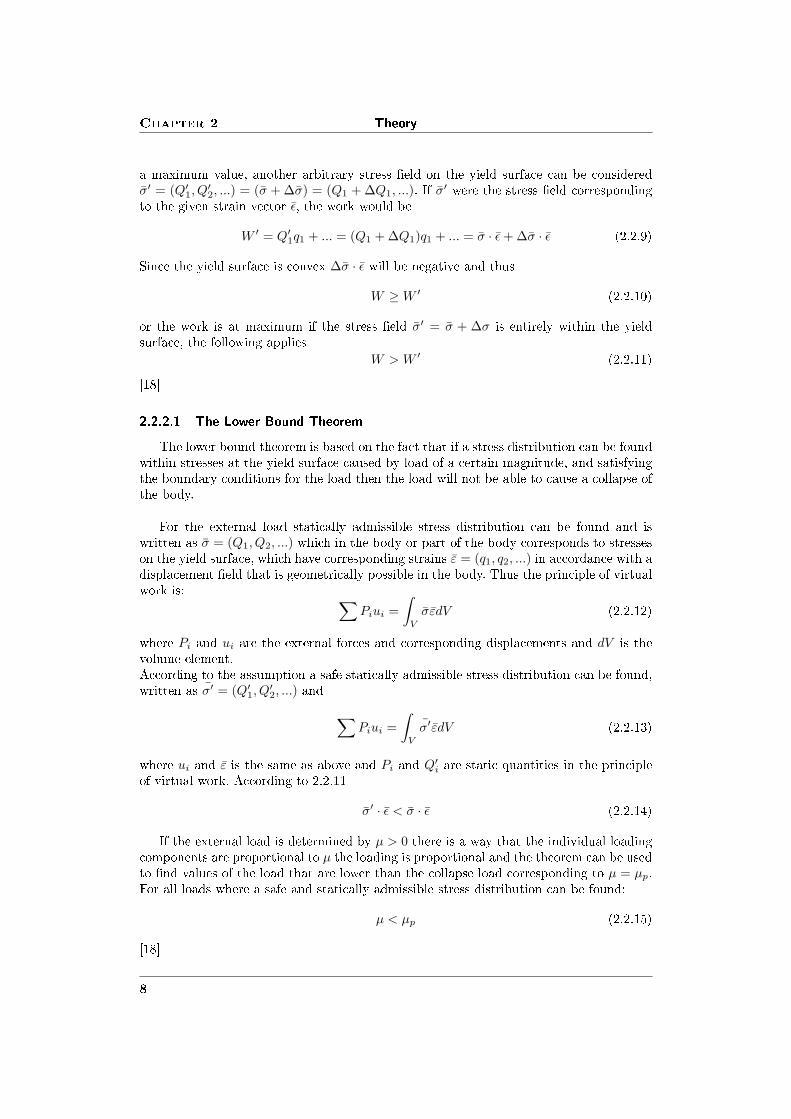
a maximum value, another arbitrary stress �eld on the yield surface can be consideredσ̄′ = (Q′1, Q
′2, ...) = (σ̄ + ∆σ̄) = (Q1 + ∆Q1, ...). If σ̄′ were the stress �eld corresponding
to the given strain vector ε̄, the work would be
W ′ = Q′1q1 + ... = (Q1 + ∆Q1)q1 + ... = σ̄ · ε̄ + ∆σ̄ · ε̄ (2.2.9)
Since the yield surface is convex ∆σ̄ · ε̄ will be negative and thus
W ≥ W ′ (2.2.10)
or the work is at maximum if the stress �eld σ̄′ = σ̄ + ∆σ is entirely within the yieldsurface, the following applies
W > W ′ (2.2.11)
[18]
2.2.2.1 The Lower Bound TheoremThe lower bound theorem is based on the fact that if a stress distribution can be found
within stresses at the yield surface caused by load of a certain magnitude, and satisfyingthe boundary conditions for the load then the load will not be able to cause a collapse ofthe body.
For the external load statically admissible stress distribution can be found and iswritten as σ̄ = (Q1, Q2, ...) which in the body or part of the body corresponds to stresseson the yield surface, which have corresponding strains ε̄ = (q1, q2, ...) in accordance with adisplacement �eld that is geometrically possible in the body. Thus the principle of virtualwork is: ∑
Piui =∫
V
σ̄ε̄dV (2.2.12)
where Pi and ui are the external forces and corresponding displacements and dV is thevolume element.According to the assumption a safe statically admissible stress distribution can be found,written as σ̄′ = (Q′
1, Q′2, ...) and
∑Piui =
∫
V
σ̄′ε̄dV (2.2.13)
where ui and ε̄ is the same as above and Pi and Q′i are static quantities in the principleof virtual work. According to 2.2.11
σ̄′ · ε̄ < σ̄ · ε̄ (2.2.14)
If the external load is determined by µ > 0 there is a way that the individual loadingcomponents are proportional to µ the loading is proportional and the theorem can be usedto �nd values of the load that are lower than the collapse load corresponding to µ = µp.For all loads where a safe and statically admissible stress distribution can be found:
µ < µp (2.2.15)
[18]
8

Design Methods Section 2.3
2.3 Design MethodsMethods based on the lower method have been developed for concrete structures and
the most obvious application consists of using the method in the design of reinforcement.Here two design methods based on the lower bound theorem will be represented.
2.3.1 Disks with Orthogonal ReinforcementGiven the stresses, σx, σy and τxy, in a disk, see Figure 2.3.
Figure 2.3: Disk element with stress in the concrete [18]
By using the given stresses the reinforcement strength needed in the x and y directionto carry them in the concrete can be calculated as ftx and fty. It is assumed that theconcrete can carry negative principal stresses in both x and y directions. At points whereone or both principal stresses are tensile stresses, reinforcement is added.The following set of formulas are used to determine the minimum reinforcement:For σx ≤ σy
Case 1:
σx ≥ −|τxy| (2.3.1)
ftx =AsxfY
t= σx + |τxy| (2.3.2)
fty =AsyfY
t= σy + |τxy| (2.3.3)
σc = 2|τxy| (2.3.4)
Case2:σx < −|τxy|
If σy < 0, reinforcement is required for
σxσy ≤ τ2xy
9

Chapter 2 Theory
And the reinforcement is determined by
Asx = 0
fty =AsyfY
t= σy +
τ2xy
|σx|σc = |σx|[1 + (
τxy
σx)2]
For σy ≤ σx
Case 1:
σy ≥ −|τxy| (2.3.5)
fty =AsyfY
t= σy + |τxy| (2.3.6)
ftx =AsxfY
t= σx + |τxy| (2.3.7)
σc = 2|τxy| (2.3.8)
Case2:σy < −|τxy|
If σx < 0, reinforcement is required for
σxσx ≤ τ2xy
And the reinforcement is determined by
Asy = 0
ftx =AsxfY
t= σy +
τ2xy
|σy|σc = |σy|[1 + (
τxy
σy)2]
where:
σx is the stresses in x direction.
σy is the stresses in y direction.
τxy is the strain.
ftx is the reinforcement strength in x direction.
fty is the reinforcement strength in y direction.
fY is the reinforcement yield strength.
Asx is the reinforcement area in x direction.
Asy is the reinforcement area in y direction.
t is the thickness of the disk.
[18]
10

Design Methods Section 2.3
2.3.2 Stringer MethodThe Stringer Method is a lower bound method, that is the load carrying capacity,
that is found with the method is equal or less than the actual load capacity. The StringerMethod can be used on all materials, where the theory of plasticity is a useful materialdescription. The method has been used for many years on steel structures and is startingto gain ground for concrete structures. It starts by looking at the wall as a disk in acoordinate system with the x as a horizontal axis and y as a vertical axis. The disk isdivided into stringers parallel with the x and y axes and the nodes where the stingerscross each other are given numbers. Between their stringers, areas are formed called meshrectangles and are given names.Figure 2.4 shows a disk which has been divided into nodes, stingers and mesh rectangleareas. One stringer goes from node to node, but a whole line of segment going from edgeto edge is called stringer line and consists of more than one stringers.
Figure 2.4: Disk divided into nodes, stringer and mesh rectangle areas[13]
When the stinger system has been made for the wall and forces been applied to it theshear stresses and stringer forces can be calculated by equilibrium equations. The mainidea is that the loads and reactions are calculated as concentrated forces in the nodes, oras shear stresses along the stringers. The stringers take on the axial stresses and can bothbe pressure- or tension stringers and the mesh rectangles take up the shear stresses, andis constant for each rectangle which means, that the force in the surrounding stringersvary linearly between the nodes.It is best to calculate �rst the shear stress in the mesh areas and thereafter the forces inthe stringers. The tension stringers need reinforcement to take up the tension force andthe reinforcement area is calculated as:
As,t =F
fyd(2.3.9)
where F is the calculated tension force in the stringer and fyd is the design yield point ofthe steel.If the calculated forces in the stringers are in compression the forces can be taken up by theconcrete supplemented with reinforcement. The calculations are based on the plasticitytheory and therefore the stress in the concrete can not be higher than the plastic strengthof the concrete, νfcd = 0.5 · 25. The stringers width is usually not bigger than 20% of the
11
Chapter 2 Theory
total mesh rectangle area length/width [7]. The needed concrete area in the stringer iscalculated as:
Ac,needed =F
νfcd(2.3.10)
where F is the compression force in the stringer, ν is the e�ciency factor and fcd is thedesign concrete strength.So the concrete can take up total force of:
C = Ac · ν · fcd (2.3.11)
where Ac is 0.2 · ′height of mesh rectangle′ ·′ wall width′
The needed reinforcement is:As,c =
F − C
fyd(2.3.12)
In the rectangle mesh areas the reinforcement is placed orthogonal and parallel with thecoordinate system or parallel with the stringers and the needed reinforcement and iscalculated as:
As =τmax · b
fyd(2.3.13)
where b is the width of the wall.[18] [13]
2.4 Finite Element AnalysisIn this project three computer programs are used, SAP2000, ETABS and ANSYS, all
based on �nite element analysis. In recent years, the use of �nite element modeling as adesign tool has grown rapidly.Here the whole content of the �nite element method or its equations will not be detailed.Only the basic part that is important for this project.
2.4.1 Basic ConceptsThe �nite element method (FEM) also called �nite element analysis (FEA) is a numer-
ical procedure that can be used to obtain solutions to a variety of problems in engineeringsuch as stress analysis, heat transfer and �uid �ow. Using programs based on FEA is verypowerful and impressive engineering tools. The method is based on that a continuous sys-tem with in�nite number of degrees of freedom (DOF) is characterized as a �nite discretemultidegree-of-freedom system, so that FEM models possessing tens of thousands of DOFare not uncommon. Several methods exist for FEA but the basic steps involved in anyFEA consist of the following:
� Create and discretize the solution domain into �nite elements; that is subdivide theproblem into nodes and elements.
� Assume a shape function to represent the physical behavior of an element; that is, acontinuous function is assumed to represent the approximate solution of an element.
� Develop equations for an element.
12

Nonlinear Analysis Section 2.5
� Assemble the elements to present the entire problem. Construct the global sti�nessmatrix.
� Apply boundary conditions, and loading.
� Solve a set of linear or nonlinear algebraic equations simultaneously to obtain nodalresults, such as displacement values at di�erent nodes.
[6]
2.5 Nonlinear AnalysisIn recent years nonlinear �nite element models have been used to utilize the behavior of
reinforced concrete. Many models have been proposed to describe this nonlinear behaviorof a reinforced concrete by using nonlinear �nite element analysis. Here the mathematicalmodels used in ANSYS will be described.
2.5.1 Concrete and SteelFigure 2.5 shows a compressive stress-strain diagram for concrete in uniaxial com-
pression. fc is the peak stress, εc1 is the strain at peak stress and εcu is the ultimatestrain.
Figure 2.5: Stress-strain diagram for concrete [9]
Figure 2.6 shows a stress-strain diagram of reinforcing steel where ft is the tensilestrength, fy the yield stress and εu the maximum elongation at maximum load
Figure 2.6: Typical stress-strain diagram of reinforcing steel [9]
13

Chapter 2 Theory
For higher grades of steel or steel strengths the tensile and yield strength gets higher.
2.5.2 Reinforced ConcreteThe characteristic stages of reinforced concrete can be illustrated by Figure 2.7 which
shows a typical load-displacement relationship. This nonlinear relationship can be dividedinto three intervals:
I The uncracked elastic stage
II Crack propagation
III The plastic stage
The last two stages or the nonlinear response is caused by cracking in the concrete andplasticity in the reinforcement and of compression in the concrete. Other time-independentnonlinearities are from the nonlinear action of the individual constituents of reinforcedconcrete, e.g., bond slip between steel and concrete, aggregate interlock of cracked concreteand dowel action of reinforced concrete. Creep, shrinkage and temperature changes, whichare all time-dependent e�ects also contribute to the nonlinear response. [21]
Figure 2.7: Typical load-displacement relationship for reinforced concreteelement [21]
2.5.3 Mathematical ModelingThe strength of concrete under multiaxial stresses is a function of the state of stress
and can not be predicted by limitations of simple tensile, compressive and shearing stressesindependently of each other. That is the strength of concrete elements can only be prop-erly determined by considering the interaction of the various components of the state ofstress. When the state of stress or strain reaches critical value, the concrete can startfailing by fracturing. The fracture of concrete can occur in two di�erent forms. One is bycracking, under tensile type of stress states, and the other by crushing under compressivetypes of stress states. The tensile weakness of concrete is a major factor contributing to
14

Nonlinear Analysis Section 2.5
the nonlinear behavior of reinforced concrete element.
The tensile weakness of concrete resulting in cracking is a major factor contributingto the nonlinear behavior of reinforced concrete. Kupfer obtained a tensile strength ofconcrete under biaxial stress states and his data provides a good de�nition of the basictensile strength of concrete under tension-tension or tension-compression biaxial stress�elds and can be seen in Figure 2.8
Figure 2.8: Biaxial strength Envelope for Plain Concrete [19]
Willam and Warnke (1975) developed a widely used model for triaxial failure surfacefor plain concrete. The failure surface is shown in Figure 2.9 where it is plotted in thecoordinate system σ1, σ2 and σ3. It is an three-dimensional stress space and is separatedinto hydrostatic and deviatoric sections. The hydrostatic section forms a meridianal planewhich contains the equisectrix σ1 = σ2= σ3 as an axis of revolution. The mathematicalmodel expresses the failure surface in terms of average or hydrostatic stress, σa (changein volume), the average shear stress, τa and the angle θ and the failure surface is de�nedas:
1z
σa
fcu+
1r(θ)
τa
fcu= 1 (2.5.1)
where z is the apex of the surface and fcu is the uniaxial compressive strength of theconcrete.The parameters that form the failure surface, z and r are identi�ed from the uniaxialcompressive strength, biaxial compressive strength and the uniaxial tension strength alongwith two points of high triaxial compression. So this representation requires �ve datapoints and the model is called the �ve parameter model of Willam and Warnke. [4] [19]
15

Chapter 2 Theory
Figure 2.9: Triaxial strength surface in principal stress space [19]
Figure 2.10 shows a typical uniaxial stress-strain curve for plain concrete up to tensileand compressive failure. For tensile failure, the behavior is essentially linearly elastic upto the failure load, the maximum stresses coincide with the maximum strains, and noplastic strains occur at the failure moment. For compressive failure, the material initiallyexhibits almost linear behavior up to the proportional limit at point A. Point A is theyielding point and before the stresses in the concrete reach that point the concrete is saidto be recoverable and can be treated within the framework of elasticity theory. After pointA only the portion εe can be recovered from the total deformation ε and the concrete isprogressively weakened by internal microcracking up to the end of the perfectly plastic�ow region CD at point D. The nonlinear deformation are basically plastic and it is clearthat the phenomenon in the region AC and in the region CD correspond exactly to thebehavior of a work hardening elastoplastic and elastic perfectly plastic solid, respectively.As can seen from Figure 2.10 the total strain ε in a plastic material can be considered asthe sum of the reversible elastic strain εe and the permanent plastic strain εp. A materialis called perfectly plastic or work-hardening according as it does or does not admit changesof permanent strain under constant stress. [21]
Figure 2.10: Typical load-displacement relationship for reinforced con-crete element [21]
16

Nonlinear Analysis Section 2.5
2.5.3.1 Elastic Based Model - Before Yielding Point
Many elasticity based models have been developed to represent the behavior of con-crete and the �eld of elasticity-based models are quite broad. They can be broken downinto subcategories based on the state of stress that is modeled (uniaxial, biaxial or tri-axial) and the form of constitutive relations (incremental or total stress-strain models).The subject in this project, the shear wall, is under biaxial loading where plane stressescan be found. For biaxial models the the most widely used representation is the isotropictotal stress-strain models. Kupfer and Gerstle devised a isotropic stress strain model forconcrete under biaxial loading based on a monotonic tests of concrete under biaxial stressand is expressed in the following form:
σx
σy
τxy
=
E
(1− ν2)
1 ν 0ν 1 00 0 (1−ν)
e
εx
εx
εx
(2.5.2)
where E is the modulus of elasticity and ν is the poisson ratio. [19]
2.5.3.2 Elastic-Strain Hardening Plastic Model - After Yielding Point
The response of the concrete after the yield point A in Figure 2.10 which is the ir-recoverable part, or the elastic-plastic response, is described by the theory of plasticity.In general models based on the plasticity describe concrete as an elastic-perfectly plasticmaterial, or to account for the hardening behavior up to the ultimate strength, as anelastic-plastic-hardening material. Here the elastic strain hardening plastic model will bedescribed, which is an approach where an initial yield surface is de�ned as the limitingsurface for elastic behavior and is located at a certain distance from the fracture (failure)surface. Figure 2.11 shows the loading surface of concrete in a biaxial stress plane for awork-hardening-plasticity model and shows the projections of the projection of the towlimiting surfaces. When the state of stress lies within the initial yield surface the materialbehavior is said to be in elastic range and linear-elastic equations can be applied. Whenthe stresses in the material go above the elastic limit surface (the yield line) a new yieldsurface called the loading surface is developed and it replaces the initial yield surface.Unloading and reloading of the material within this subsequent loading surface resultsin elastic behavior and no additional irrecoverable deformation will occur until this newsurface is reached. If further discontinuity is continued beyond this surface a �nal collapseof the concrete cracking or crushing occurs, depending on the nature of the stress state.
17

Chapter 2 Theory
Figure 2.11: Loading surfaces of concrete in biaxial stress plane for awork-hardening-plasticity model [4]
The formulation of the constitutive relations for a strain-hardening plastic material isbased on three fundamental assumptions:
1. The shape of an initial yield surface
2. The evolution of subsequent loading surface (or hardening rule)
3. The formulation of an appropriate �ow rule.
[4] [19]
2.5.3.3 The Shape of an Initial Yield SurfaceThere exists a loading function f which depends upon the state of stress and strain and
the history of loading. In other words, at each stage of a plastic deformation or unloading,there is some function of stress f(σij) such that no additional plastic deformations takeplace when f is smaller than some number k and plastic �ow of a work-hardening materialoccurs when f exceeds k. That is f is dependent of state of stress, the plastic strains andthe hardening parameter:
f = f(σij , εpij , k) (2.5.3)
So di�erent material states can be de�ned:
� f = 0 represents yield states.
� f < 0 elastic behavior occurs.
[4]
18
Nonlinear Analysis Section 2.5
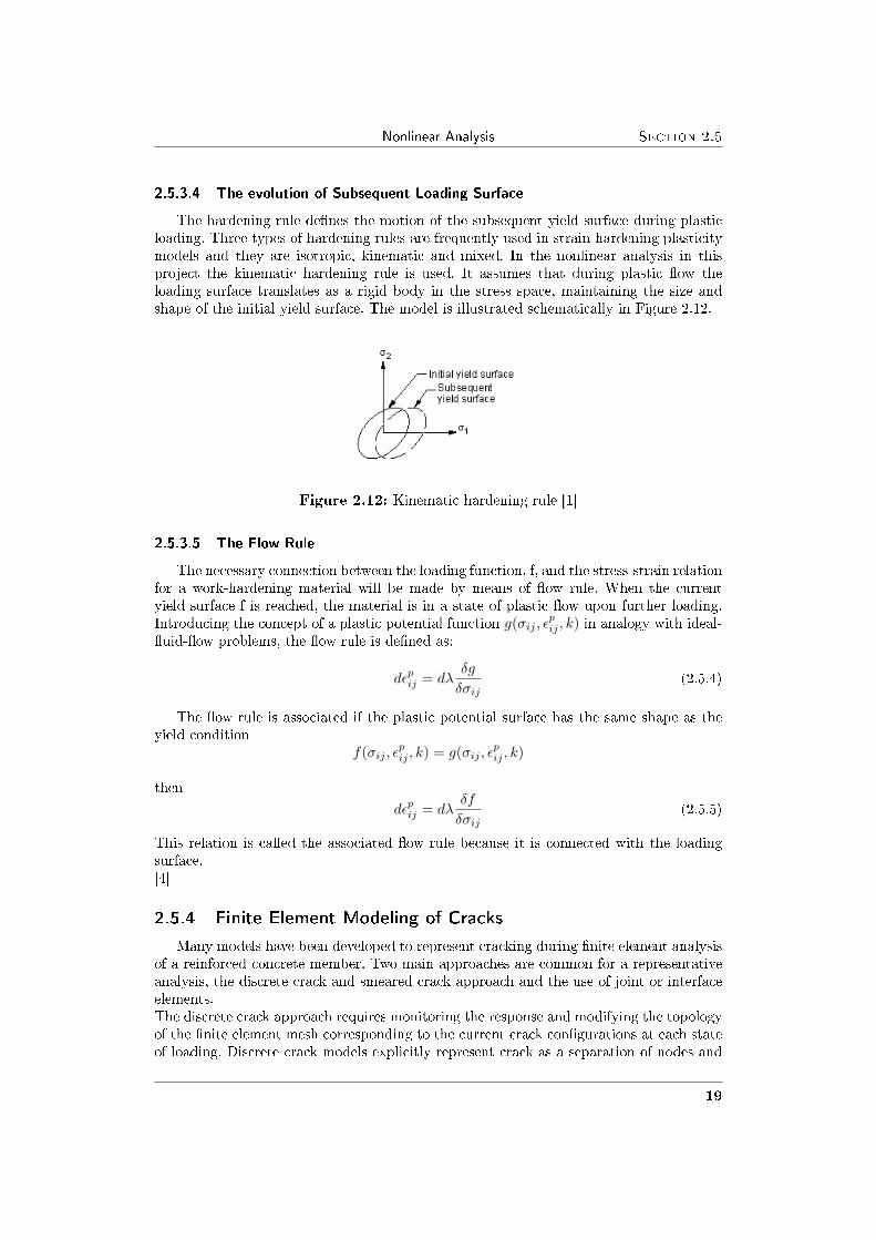
2.5.3.4 The evolution of Subsequent Loading SurfaceThe hardening rule de�nes the motion of the subsequent yield surface during plastic
loading. Three types of hardening rules are frequently used in strain-hardening plasticitymodels and they are isotropic, kinematic and mixed. In the nonlinear analysis in thisproject the kinematic hardening rule is used. It assumes that during plastic �ow theloading surface translates as a rigid body in the stress space, maintaining the size andshape of the initial yield surface. The model is illustrated schematically in Figure 2.12.
Figure 2.12: Kinematic hardening rule [1]
2.5.3.5 The Flow RuleThe necessary connection between the loading function, f, and the stress-strain relation
for a work-hardening material will be made by means of �ow rule. When the currentyield surface f is reached, the material is in a state of plastic �ow upon further loading.Introducing the concept of a plastic potential function g(σij , ε
pij , k) in analogy with ideal-
�uid-�ow problems, the �ow rule is de�ned as:
dεpij = dλ
δg
δσij(2.5.4)
The �ow rule is associated if the plastic potential surface has the same shape as theyield condition
f(σij , εpij , k) = g(σij , ε
pij , k)
thendεp
ij = dλδf
δσij(2.5.5)
This relation is called the associated �ow rule because it is connected with the loadingsurface.[4]
2.5.4 Finite Element Modeling of CracksMany models have been developed to represent cracking during �nite element analysis
of a reinforced concrete member. Two main approaches are common for a representativeanalysis, the discrete crack and smeared crack approach and the use of joint or interfaceelements.The discrete crack approach requires monitoring the response and modifying the topologyof the �nite element mesh corresponding to the current crack con�gurations at each stateof loading. Discrete crack models explicitly represent crack as a separation of nodes and
19

Chapter 2 Theory
the node is rede�ned as two nodes. Having many cracks leads to many degrees of freedomand the mesh topology of the problem may have to be changed signi�cantly to cope withnew crack patterns. Therefore the discrete crack approach may not be the best choicefor problems with many cracks, like in reinforced concrete elements. These problemscan mostly be avoided in the smeared crack approach, which models cracks and jointsin an average sense by appropriately modifying material properties at the integrationpoints of regular �nite elements. The formation of a crack involves no remeshing or newdegrees of freedom. However they have limited ability to model sharp discontinuities andrepresent the topology or material behavior in the vicinity of the crack. The smearedcrack approach works best when cracks to be modeled are themselves smeared out, as inreinforced concrete applications. [16]
2.6 DuctilityTo minimize major damage and to ensure the survival of buildings with moderate
resistance with respect to lateral force, structures must be capable of sustaining a highproportion of their initial strength when a major earthquake imposes large deformations.These deformations may be well beyond the elastic limit. This ability of the structureor its components, or of the materials used to o�er resistance in the inelastic domain ofresponse, is described by the general term ductility. It includes the ability to sustain largedeformations, and a capacity to absorb energy by hysteric behavior.The ductility is de�ned as the ratio of the total imposed displacements ∆ at any instantto that at the onset of yield ∆y.
µ =∆∆y
> 1 (2.6.1)
The ductility, µ, of a structure, that is the ductility developed when failure is imminentis:
µu =∆u
∆y(2.6.2)
The displacements ∆u and ∆y may represent strain, curvature, rotation or de�ection,where the de�ection is the most convenient quantity to evaluate either the ductility im-posed on a structure by earthquake µm or the structures's capacity to develop ductility µu.
Ductility is the structural property that will need to be relied on in most buildingsif satisfactory behavior under damage control and survival limit state is to be achieved.An important consideration in the determination of the required seismic resistance willbe that the estimated maximum ductility demand during shaking does not exceed theductility potential µu. It is possible to satisfy the performance criteria of the damagecontrol and survival limit state by one of the three distinct design approaches, related tothe level of ductility permitted of the structure. An illustration of these three approachesare shown in Figure 2.13 where the strength SE , required to resist earthquake-inducedforces and structural displacements ∆ at the development at di�erent levels of strengthare related to each other.
20

Cracks Section 2.7
Figure 2.13: Relationship between strength and ductility [21]
a Elastic response. Because of their great importance, certain buildings will deed topossess adequate strength to ensure that they remain essentially elastic. Other struc-tures, perhaps of lesser importance, may nevertheless possess a level of inherentstrength such that elastic response is assured. The idealized response of such struc-ture is shown in Figure 2.13 by the bilinear strength-displacement path OAA′. Themaximum displacement ∆me is very close to the displacement of the ideal elasticstructure.
b Ductile response. Most ordinary buildings are designed to resist lateral seismic forcewhich are smaller than those that would be developed in an elastically respondingstructure as Figure 2.13 shows, that inelastic deformation and hence ductility willbe required of the structure. These structures can be divided into two groups.
1. Fully ductile structures; These are designed to possess the maximum ductilitypotential than can reasonably be achieved at carefully identi�ed and detailedinelastic regions. The idealized bilinear response of this type of structure isshown in Figure 2.13 by the path OCC ′
2. Structures with Restricted Ductility ; Certain structures inherently possess sig-ni�cant strength with respect to lateral forces as a consequence, for example,of the presence of large areas of structural walls.
Figure 2.13 shows approximate values of ductility factors which may be used as guidesfor the limit of the categories discussed. Although displacement ductilities in excess of8 can be developed in some well-detailed reinforced concrete structures, the associatedmaximum displacements ∆mf are likely to be beyond limits set by other design criteria,such as structural stability. Elastically responding structures, implying no or negligibleductility demands, represent the other limit.[21]
2.7 CracksCracking should be limited to a level that will not impair the proper functioning of
the structure or cause its appearance to be unacceptable, it is also important from the
21
Chapter 2 Theory
aesthetic view to control the cracking.
Concrete cracks early in its loading history. Most cracks are results from the followingactions.
1. Volumetric change caused by plastic shrinkage or expensive chemical reactionswithin hardened concrete,creep and thermal stresses.
2. Stress because of bending, shear or other moments caused by transverse loads.
3. Direct stress due to applied loads or reactions or internal stresses due to continuity,reversible fatigue load, long-term de�ection, environmental e�ects or di�erentialmovements in structural system.
While the net results of these three actions cause the formation of cracks, the mechanismof their development cannot be considered identical. Volumetric change cause internalmicro-cracking, which may develop into full cracking. This project deals with formationsof cracks from the second and the third action where external loads results in direct andbending stresses causing �exural, bond and diagonal tension cracks. As the tensile stressin the concrete exceeds its tensile strength, internal micro-cracks form. These cracks de-velop into macro-cracks propagating to the external �ber zone of the element.
The maximum crack width that a structural element should be permitted to developdepends on the particular function of the element and the environmental condition towhich the structure is liable to be subjected. Icelandic houses are usually in exposureclass 2b (according to EC2) meaning that the environment is humid and frost occurs andfor corrosion protection to the reinforcement, the limitation of the maximum design crackwidth is about 0.3 mm
[9][17]
2.8 Methods to Calculate CracksThe design provision at the ultimate limit states may lead to excessive stresses in the
concrete and the reinforcing steel. These stresses may, as consequence, adversely a�ectthe appearance and performance in service conditions and the durability of concretestructures.
2.8.1 Calculation of design crack widthsThe design crack width may be obtained from EC2:4.4.2.4 from the relation:
wk = β · srm · εsm (2.8.1)
where:wk is the design crack width.srm is the average �nal crack spacing.εsm is the mean strain allowed under the relevant combination of loads for the e�ects oftension sti�ening, shrinkage, etc.β is a coe�cient relating the average crack width to the design value and here it may be
22

Shear Wall Section 2.9
taken as 1.3 or 1.7.εsm may be calculated from the relation:
εsm =σs
Es(1− β1β2(
σsr
σs)2) (2.8.2)
where:σs is the stress in the tension reinforcement calculated on the basis of a cracked section.σsr is the stress in the tension reinforcement calculated in the basis of a cracked sectionunder the loading conditions causing the �rst cracking.β1 is a coe�cient which takes account of the bond properties of the bars, 1 for high bondbars and 0.5 for plain bars.β2 is a coe�cient which takes account of the duration of the loading or of repeated loading,1 for a single short term loading and 0.5 for a sustained load or for many cycles of repeatedloading.The average �nal crack spacing for members subjected dominantly to �exure or tensioncan be calculated with the equation:
srm = 50 + 0.25k1k2φ/pr (2.8.3)
where:φ is the bar size in mm. Where mixture of bar sizes is used in section, an average bar sizemay be used.k1 is a coe�cient which takes account of the bond properties of the bars;k2 is a coe�cient which takes account of the form of the strain distribution.
[9]
2.9 Shear WallShear walls are commonly put into multi-storey buildings because of their good per-
formance under lateral loads like earthquake forces because they provide lateral stabilityand they act as vertical cantilevers in resisting the horizontal forces.The shear wall that is considered in this project if shown in Figure 2.14. It is a three storywall with one door on the ground �oor and 8 windows.
Figure 2.14: The Shear Wall
23

Chapter 2 Theory
Sti�ness, strength and ductility are the basic criteria that the structure should satisfyand shear walls provide a nearly optimum means of achieving those objectives. Buildingshaving shear walls are sti�er than framed structures resulting in reduced deformationsunder earthquake load. The necessary strength to avoid damage in the structure can beachieved by properly detailed longitudinal and transverse reinforcement and providingthat special detailing measures are adopted, dependable ductile response can be achievedunder major earthquakes.Structural walls usually have openings, in this project the openings are that big that theycan not be neglected in the design computations because they a�ect the shear and �exuralstrength of the wall.
Walls of the type shown in Figure 2.15, and of the same type as the wall analyzedhere, are characterized by a small height-to-length ratio, hw/lw. The potential �exuralstrength of such walls may be very large in comparison with lateral forces. Because of thesmall height, relatively large shearing forces must be generated
Figure 2.15: Structural wall [21]
To accommodate large seismically induced deformations, most structures need to beductile. Thus in the design of structures for ductile, it is preferable to consider forcesgenerated by earthquake-induced displacements rather than traditional loads.[21]
24

Chapter 3
The Building and the Load
In this chapter the analyzed building is described, the total mass calculated and theapplied load from an earthquake on the building is calculated. The house is a three storyo�ce building, it does not exist in reality and it is assumed that it is placed on the Southpart of Iceland.
3.1 The BuildingDrawings of the building is shown in �gures 3.1 and 3.2. The building is a RC structure
with windows all of the same size and it is assumed that the roof is monotonic made ofconcrete. Figure 3.2 shows the geometry of the wall analyzed, it has eight windows andone door. Openings are 23% of the area and height versus length (H/L) ratio is 0.78.The concrete strength is C30/35 and the wall thickness is 200 mm. The dimensions andparameters of the building can be seen in �gures 3.1 and 3.2 and Table 3.1.
Figure 3.1: Plan View
25

Chapter 3 The Building and the Load
Figure 3.2: The Shear Wall Dimensions
The following parameters are given regarding the structure:
Table 3.1: The buildings parametersBuilding height H=9.0 [m]Building width W=20 [m]Building depth (shear wall) L=11.5 [m]Story height h=3.0 [m]Wall thickness tw=200 [mm]Floor slab/roof thickness ts=200 [mm]Density of concrete ρc=2500 [kg/m3]Density of glass ρc=2600 [kg/m3]Thickness of double glass tg=0.008 [m]Young's modulus for concrete Ec = 3.4 · 1010 [N/m2]Dead and live loading on each story q = 5000 [N/m2]Concrete strength C30Reinforcement strength 500 MPa
3.1.1 The Mass of the BuildingEven thought that in this project only one wall of the building is analyzed the weight
of the whole building has to be calculated to be able to calculate the total earthquakeforce applied on the wall. Figure 3.3 shows the dimensions of the longitudinal wall.
26

The Building Section 3.2
Figure 3.3: The Longitudinal Wall Dimensions
The mass of the total building is:
The shear wall : 2 · 0.2 · 9 · 11.5 = 41.4 m3
Longitudinal wall : 2 · 0.2 · 9 · 20 = 72 m3
Roof and slabs : 3 · 0.2 · 11.5 · 20 = 138 m3
Openings:
Shear wall windows : = 2 · 8 · 0.2 · 2.5 · 1.2 = 9.6 m3
Shear wall door : = 2 · 0.2 · 1 · 2.2 = 0.88 m3
Longitudinal wall windows : = 2 · 15 · 0.2 · 2.5 · 1.25 = 18 m3
Total volume of concrete
⇒ 41.4 + 72 + 138− 9.6− 0.88− 18 = 223 m3
The total mass of the concrete:
223m3 · 2500kg/m3 = 557300kg
Mass of the glass:
(2 · (1 · 2.2 + (8 + 15) · 2.5 · 1.2) · 0.008 = 1.14m3 ⇒ 1.14m3 · 2600kg/m3 = 2962kg
The total mass of the building
557300 + 2962 = 560261kg
Mass for each story:m1=150877 kgm2=186754 kgm3=186754 kg
27

Chapter 3 The Building and the Load
3.2 Pushover AnalysisPushover analysis is non-linear static approach carried out under constant gravity
loads and by subjecting monotonically increasing lateral forces. The forces are applied atthe location of the masses in the structural model, representing the inertial forces whichwould be experienced by the structure when subjected to ground shaking.Three basic methods are used in seismic analysis to estimate the response of the buildingand the internal forces.
1. Methods that are based on equivalent lateral force.
2. Methods based on multi modal response analysis.
3. Methods based on non-linear time history analysis.
The �rst method uses a static force which is distributed on the building according tospeci�c rules listed in EC8. This method is good for simple regular buildings and couldtherefore be applied for the three story shear wall.
3.2.0.1 Lateral Force PatternsThe selection of an appropriate lateral load distribution is important within the
pushover analysis. In EC8 the non-linear static procedure requires at least two force dis-tributions, a uniform and modal pattern. The uniform pattern is with lateral forces thatare proportional to masses and the modal pattern varies with change in de�ected shapeas it yields or more precise from EC8:4.3.3.4.2.2, pushover analysis should be performedusing both of the following lateral load patterns:
1. A "uniform" pattern, based on lateral forces that are proportional to mass regardlessof elevation (unform response acceleration);
2. A "modal" pattern, which depends on the type of linear analysis applicable to theparticular structure. Because the building satis�es the condition for the applicationof lateral force analysis method, an 'inverted triangular' unidirectional force pattern,similar to the one used in that method is used.
The most unfavorable result of the pushover analysis using the two standard lateral forcepatterns should be adopted. Moreover, unless there is perfect symmetry with respect toan axis orthogonal to that of the seismic action components considered, each lateral forcepattern should be applied in both the positive and the negative direction, and the resultused should be the most unfavorable one from the two analyses.In this thesis only the second load pattern is used in the static pushover analysis.
3.2.0.2 Capacity CurveThe key outcome of the pushover analysis is the 'capacity curve', i.e. the relation
between the base shear force, Fb, and the representative lateral displacement of the struc-ture, dn. That displacement is often taken at a certain node n of the structural model,termed the control node. The control node is normally at the roof level.[10] [12]
28

Load - Lateral Force Method of Analysis Section 3.3
3.3 Load - Lateral Force Method of AnalysisIn the lateral force method a linear static analysis of the structure is performed under
a set of lateral forces applied separately in two orthogonal horizontal directions, x andy. The intent is to simulate through these forces the peak inertia load induced by thehorizontal component of the seismic action in the two directions, x and y. Owing to thefamiliarity and experience of structural engineers with elastic analysis for static loads(due to gravity, wind or other static actions), this method has long been - and still is -the workhorse for practical seismic design.
3.3.1 Can the Lateral Force Method be used?According to EC8:4.3.3.2.1(1)P the lateral force method can be applied to buildings
whose response is not signi�cantly a�ected by contributions from modes of vibrationhigher than the fundamental mode in each principal direction.The fundamental period of vibration, T1, in the two main directions should be smallerthan:
T1 ≤{
4 · Tc = 4 · 0.4 = 1.6s,2.0s
(3.3.1)
Where Tc = 0 is found in EC8, Table 3.2, and the building shall meet the criteria forregularity in elevation, given in EC8: 4.2.3.3.
According to EC8: 4.3.3.2.2 the seismic base shear force, Fb for the horizontal direction
Fb = Sd(T1) ·m · λ (3.3.2)
whereSd(T1) is the ordinate of the design spectrum at period T1. (See EC8: 3.2.2.5)m is the total mass of the building, computed in accordance with EC8:3.2.4(2)λ is the correction factor, here λ = 0.85 if T1 ≤ 2Tc and the building has more than twostories.
T1 can be approximated:T1 = Ct ·H3/4 (3.3.3)
where Ct = 0.075√Ac
- for a concrete shear wall and Ac is the total e�ective area of the shearwall.Ac is given by the equation:
Ac =∑
[Ai · (0.2 + (lwi/H))2] (3.3.4)
Where Ai is the e�ective cross sectional area of the shear wall i in the �rst storey of thebuilding in m2.lwi is the length of the shear wall i in the �rst storey in the direction parallel to theapplied forces, in m,.H is the height of the building, in m, from the foundation or the top of the rigid basementand lwi/H should not exceed 0.9.
29

Chapter 3 The Building and the Load
It is assumed that the building has two opposite shear walls.Ai = 11.5m · 0.2m = 2.3m2
From 3.3.4 Ac = 2 · (2.3 · (0.2 ·+0.92)) = 2.323Then Ct can be calculated:
Ct =0.075√2.323
= 0.049
Finally the �rst period is calculated from 3.3.3
T1 = 0.049 · 93/4 = 0.256
See if it �ts the requirements from 3.3.1
T1 = 0, 256s ≤{
4 · Tc = 4 · 0.4 = 1.6s,2.0s
Therefore the lateral force method of analysis can be used.[10]
3.3.2 The Design Response SpectraTo calculate the seismic base shear force the shape of the design response spectra is
needed.The building is placed on the South Iceland Seismic Zone (SISZ). The horizontal groundacceleration for Iceland according to the Icelandic National Annex FS ENV 1998-1-1:1994can be seen in Figure 3.4. The ground acceleration is 0.4g.
Figure 3.4: Horizontal ground acceleration for Iceland
Usually houses in Iceland are built on solid rock or ground type A. The importanceclass is set to III, which is for ordinary buildings not belonging to the other three im-portance classes, see EC8: Table 4.3. The following parameters (in Table 3.2) are used to
30

Load - Lateral Force Method of Analysis Section 3.3
calculate the shape of the design response spectra:
Table 3.2: Parameters for design response spectraGround type AImportance class III → γ1 = 1 (the important factor)Ground acceleration ag = 0.4gBehavior factor q = q0kw ≥ 1.5
According to EC8:5.2.2.2 q0 is the basic value dependent on the type of the structuralsystem and on its regularity in elevation. The building has Ductility Class Medium (DCM)so q0 = 3
kw =(1 + α0)
3≤ 1but not less than 0.5
α0 =∑
hwi∑lwi
=2 · 9
2 · 11.5= 0.78
The behavior factor can then be calculated
q = 3 · 0.59 = 1.78
From EC8 3.2.2.5 the horizontal design response spectrum, Sd(T ), is de�ned by thefollowing expression:
0 ≤ T ≤ TB : Sd(T ) = ag · S · [ 23 +T
TB· (2.5
q− 2
3)]
TB ≤ T ≤ TC : Sd(T ) = ag · S · 2.5q
TC ≤ T ≤ TD : Sd(T ) ={
ag · S · 2.5q · [TC
T ]≥ β · aq
TD ≤ T : Sd(T ) ={
ag · S · 2.5q · [TCTD
T 2 ]≥ β · aq
T is the vibration period of a linear single-degree-of-freedom system. The designground acceleration according to EC8.3.2.1(3)is:
ag = γI · agR = 1 · 0.4 · 9.81 = 4.12m/s2 (3.3.5)
TB , TC are the limits of the constant spectral acceleration branch and TD is the valuede�ning the beginning of the constant displacement response range of the spectrum.S is the soil factor.The damping correction factor is η, with reference value η = 1 for 5% viscous damping.The following values in Table 3.3 are de�ned and describe the recommended type 1 designresponse spectrum for type A ground, see EC 8: Table 3.2
31

Chapter 3 The Building and the Load
Table 3.3: Parameters for type 1 design response spectrum.S = 1TB(S) = 0.15TC(S) = 0.4TD(S) = 2.0
The horizontal design spectrum is evaluated in MATLAB and the script can be seenin appendix A and the shape of the design response spectrum in Figure 3.5.
0 0.5 1 1.5 2 2.5 3 3.5 40
0.5
1
1.5The response spectrum for ζ = 0.05
T
Sdh
/ag
Figure 3.5: Horizontal design spectrum
From Figure 3.5 it can be seen that for T1 = 0.256
Sd(T1)ag
= 1.068 ⇒ Sd(T1) = 1.404 · 0.4 · 9.81 · 1 = 5.5m/s2
Use EC8:4.3.3.2.3 to distribute the horizontal seismic forces:According to 4.3.3.2.3(3) the fundamental mode shape is approximated by horizontaldisplacements increasing linearly along the height, the horizontal forces, Fi, should betaken as being given by:
Fi = Fb · zi ·mi∑zj ·mj
(3.3.6)
wheremi, mj are the storey masses.zi, zj are the heights of the masses, mi, mj , above the level of application of the seismicaction.The mass is computed in accordance with EC8:3.2.4(2)
mi = ΣGk,j” + ”∑
ΨE,i ·Qk,i (3.3.7)
32

Load - Lateral Force Method of Analysis Section 3.3
whereΨE,i is the combination coe�cient for variable action i and is computed from the follow-ing expression ΨE,i = ϕ ·Ψ2i, here ϕ = 0.5 and Ψ2i = 0.3
Here live load is set to 3kN/m2 (o�ce building) and dead load (furniture etc.) to2kN/m2 on each story.
m1 = 150877kg
m2 = 186754 +2000 · 20 · 11.5
9.81+ 0.3 · 0.5
·3000 · 10 · 11.59.81
= 244195kg
m3 = 244195kg
Total mass, m=639268 kgSo from eq. 3.3.2 the seismic base shear force is:
Fb = 5.5 · 636683 · 0.85 = 2989kN
∑zj ·mj = 9 · 150877 + 6 · 244195 + 3 · 244195 = 3555648kg
Which gives:
F1 = 2989 · 9 · 1508773555648
= 1141kN
F2 = 2989 · 6 · 2431503555648
= 1226kN
F3 = 2989 · 3 · 2431503555648
= 613kN
The loads F1, F2 and F3 are divided on two shear walls (i.e. one in each end of thebuilding) and the load acting on shear wall to be analysed is therefore:
F1 = 570kN
F2 = 613kN
F3 = 307kN
3.3.3 Vertical LoadSafety factor for permanent action is 1.35 and 1.5 for variable action:
Weight from the roof:1.35 · 1
3 · 20m · 0.2m · 25kN/m3 = 45kN/mWeight from the �oor with live and dead load:45kN/m + 1.35 · 3 · 1
3 · 20 + 1.35 · 2 · 13 · 20m = 92kN/m
Weight from the shear wall:1.35 · 3m · 0.2m · 11.525kN/m3 = 0.81kN/mLoad on top: 45kN/mLoad on second �oor: 138kN/m
33

Chapter 3 The Building and the Load
Load on �rst �oor: 138kN/m
The load applied on the shear wall can be seen in Figure 3.6.
Figure 3.6: Forces applied on the shear wall
34

Chapter 4
Reinforcement Design
4.1 The Stringer MethodThe Stringer method is explained in section 2.3.2. It starts by dividing the wall into
stingers, nodes and rectangle mesh areas. The nodes are given numbers from 1 to 86 andthe areas are marked from x1 to x18. When marking the areas the thought was due tosymmetry of the wall that some of the mesh rectangles are assumed to have the sameshear stress. There are eighteen unknown values so eighteen equations have to be createdto be able to �nd the shear stress in each mesh rectangle. Here the line containing nodeone to eight is called stringer line 1, node 9 to 16 stringer line 2 and etc. This con�gurationcan be seen in Figure 4.1
4.1.1 The LoadIn chapter 3.3.2 and 3.3.3 the load acting on the shear wall was calculated. For the
wall to be in equilibrium, moments from the forces are calculated and loads put on thewall to balance it. That is for the three calculated horizontal loads acting on the building,forces are acting upon the wall so the set of the loads acting on the wall is zero.The moment acting on the building from the calculated horizontal loads:
570kN · 9m + 613kN · 6m + 307kN · 3m = 9729kNm
Forces acting against the horizontal loads are applied at the vertical stringer lines andare calculated as:
9729 = 2 · P · (5.75 +4.752
5.75+
2.252
5.75+
1.252
5.75) ⇒ P = 449kN
449 · 4.755.75
= 370kN
449 · 2.255.75
= 175kN
449 · 1.255.75
= 98kN
The applied forces for the calculations in the stringer method are shown in Figure 4.2.
35

Chapter 4 Reinforcement Design
Figure 4.1: The wall divided into nodes, stringers and areas
Figure 4.2: The forces acting on the wall for Stringer Method
36
The Stringer Method Section 4.1
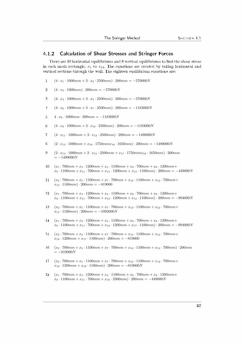
4.1.2 Calculation of Shear Stresses and Stringer ForcesThere are 10 horizontal equilibriums and 8 vertical equilibriums to �nd the shear stress
in each mesh rectangle, x1 to x18. The equations are created by taking horizontal andvertical sections through the wall. The eighteen equilibrium equations are:
1 (4 · x1 · 1000mm + 3 · x2 · 2500mm) · 200mm = −570000N
2 (4 · x3 · 1000mm) · 200mm = −570000N
3 (4 · x4 · 1000mm + 3 · x5 · 2500mm) · 200mm = −570000N
4 (4 · x6 · 1000mm + 3 · x7 · 2500mm) · 200mm = −1183000N
5 4 · x8 · 1000mm · 200mm = −1183000N
6 (4 · x9 · 1000mm + 3 · x10 · 2500mm) · 200mm = −1183000N
7 (4 · x11 · 1000mm + 3 · x12 · 2500mm) · 200mm = −1490000N
8 (2 · x13 · 1000mm + x16 · 1750mmx18 · 1650mm) · 200mm = −1490000N
9 (2 · x14 · 1000mm + 2 · x15 · 2500mm + x17 · 1750mmx18 · 1650mm) · 200mm= −1490000N
10 (x1 · 700mm + x3 · 1200mm + x4 · 1100mm + x6 · 700mm + x8 · 1200mm+x9 · 1100mm + x11 · 700mm + x13 · 1200mm + x14 · 1100mm) · 200mm = −449000N
11 (x2 · 700mm + x5 · 1100mm + x7 · 700mm + x10 · 1100mm + x12 · 700mm+x15 · 1100mm) · 200mm = −819000
12 (x1 · 700mm + x3 · 1200mm + x4 · 1100mm + x6 · 700mm + x8 · 1200mm+x9 · 1100mm + x11 · 700mm + x13 · 1200mm + x14 · 1100mm) · 200mm = −994000N
13 (x2 · 700mm + x5 · 1100mm + x7 · 700mm + x10 · 1100mm + x12 · 700mm+x15 · 1100mm) · 200mm = −1092000N
14 (x1 · 700mm + x3 · 1200mm + x4 · 1100mm + x6 · 700mm + x8 · 1200mm+x9 · 1100mm + x11 · 700mm + x16 · 1200mm + x17 · 1100mm) · 200mm = −994000N
15 (x2 · 700mm + x5 · 1100mm + x7 · 700mm + x10 · 1100mm + x12 · 700mm+x16 · 1200mm + x17 · 1100mm) · 200mm = −819000
16 (x2 · 700mm + x5 · 1100mm + x7 · 700mm + x10 · 1100mm + x12 · 700mm) · 200mm= −819000N
17 (x2 · 700mm + x5 · 1100mm + x7 · 700mm + x10 · 1100mm + x12 · 700mm+x18 · 1200mm + x18 · 1100mm) · 200mm = −819000N
18 (x1 · 700mm + x3 · 1200mm + x4 · 1100mm + x6 · 700mm + x8 · 1200mm+x9 · 1100mm + x11 · 700mm + x18 · 2300mm) · 200mm = −449000N
37

Chapter 4 Reinforcement Design
Matlab is used to solve these equations and are put into the matrices A and b as seenbelow:
A=200*[4*1000 3*2500 0 0 0 0 0 0 0 0 0 0 0 0 0 0 0 0;0 0 4*1000 0 0 0 0 0 0 0 0 0 0 0 0 0 0 0;0 0 0 4*1000 3*2500 0 0 0 0 0 0 0 0 0 0 0 0 0;0 0 0 0 0 4*1000 3*2500 0 0 0 0 0 0 0 0 0 0 0;0 0 0 0 0 0 0 4*1000 0 0 0 0 0 0 0 0 0 0;0 0 0 0 0 0 0 0 4*1000 3*2500 0 0 0 0 0 0 0 0;0 0 0 0 0 0 0 0 0 0 4*1000 3*2500 0 0 0 0 0 0;0 0 0 0 0 0 0 0 0 0 0 0 2*1000 0 0 1750 0 1750;0 0 0 0 0 0 0 0 0 0 0 0 0 2*1000 2*2500 0 1750 1750;700 0 1200 1100 0 700 0 1200 1100 0 700 0 1200 1100 0 0 0 0;0 700 0 0 1100 0 700 0 0 1100 0 700 0 0 1100 0 0 0;700 0 1200 1100 0 700 0 1200 1100 0 700 0 1200 1100 0 0 0 0;0 700 0 0 1100 0 700 0 0 1100 0 700 0 0 1100 0 0 0;700 0 1200 1100 0 700 0 1200 1100 0 700 0 0 0 0 1200 1100 0;0 700 0 0 1100 0 700 0 0 1100 0 700 0 0 0 1200 1100 0;0 700 0 0 1100 0 700 0 0 1100 0 700 0 0 0 0 0 0;0 700 0 0 1100 0 700 0 0 1100 0 700 0 0 0 0 0 2300;700 0 1200 1100 0 700 0 1200 1100 0 700 0 0 0 0 0 0 2300];
b= [-570000;-570000-570000-1183000-1183000-1183000-1490000-1490000-1490000-449000-819000-994000-1092000-994000-819000-819000-819000-449000];
Unfortunately the matrices do not have a unique solution. But one of the solutions canbe found by using the MATLAB function x = pinv(A) ∗ b to solve x1 to x18, the pinvfunction is an expensive way to calculate the inverse of matrix. The results are shown inTable 4.1, the shear stresses for the �rst nine mesh rectangles are acceptable and their
38
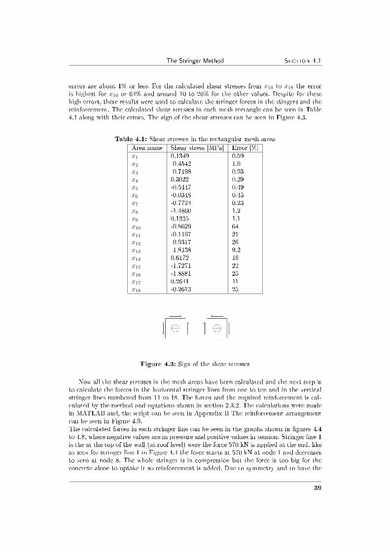
The Stringer Method Section 4.1
errors are about 1% or less. For the calculated shear stresses from x10 to x18 the erroris highest for x10 or 64% and around 10 to 20% for the other values. Despite for thesehigh errors, these results were used to calculate the stringer forces in the stingers and thereinforcement. The calculated shear stresses in each mesh rectangle can be seen in Table4.1 along with their errors. The sign of the shear stresses can be seen in Figure 4.3.
Table 4.1: Shear stresses in the rectangular mesh areasArea name Shear stress [MPa] Error [%]x1 0.1349 0.59x2 -0.4542 1.0x3 -0.7198 0.93x4 0.3022 0.29x5 -0.5447 0.49x6 -0.0348 0.45x7 -0.7724 0.23x8 -1.4860 1.2x9 0.1325 1.1x10 -0.8629 64x11 -0.1197 21x12 -0.9317 26x13 -1.8138 9.2x14 0.6172 16x15 -1.7271 22x16 -1.8881 25x17 0.2641 11x18 -0.2613 25
Figure 4.3: Sign of the shear stresses
Now all the shear stresses in the mesh areas have been calculated and the next step isto calculate the forces in the horizontal stringer lines from one to ten and in the verticalstringer lines numbered from 11 to 18. The forces and the required reinforcement is cal-culated by the method and equations shown in section 2.3.2. The calculations were madein MATLAB and, the script can be seen in Appendix B The reinforcement arrangementcan be seen in Figure 4.9.The calculated forces in each stringer line can be seen in the graphs shown in �gures 4.4to 4.8, where negative values are in pressure and positive values in tension. Stringer line 1is the at the top of the wall (at roof level) were the force 570 kN is applied at the end, likeas seen for stringer line 1 in Figure 4.4 the force starts at 570 kN at node 1 and decreasesto zero at node 8. The whole stringer is in compression but the force is too big for theconcrete alone to uptake it so reinforcement is added. Due to symmetry and to have the
39

Chapter 4 Reinforcement Design
reinforcement simplest as possible the reinforcement is the same for the whole stringerline and is put as 4k16. No force is acting on stringer line 2 and therefore the force is zeroat node 9 and 16, the force shifts between tension and compression along the stringer line.The predominant force is used to calculate the needed reinforcement and again becauseof symmetry and making the reinforcement simple the same reinforcement is put in thewhole stringer line. The same approach is made for stinger lines 3, 5, 6, 8, 9 and 10.
1 2 3 4 5 6 7 8−600
−400
−200
0
200
stringerline no 1
Horizontal stringer forces
9 10 11 12 13 14 15 16−200
−100
0
100
200
Str
inge
rfor
ce [k
N]
stringerline no 2
17 18 19 20 21 22 23 24−400
−200
0
200
400
stringerline no 3
Figure 4.4: Horizontal Stringer Forces for stringerline 1 to 3
The force 613 kN is applied at the end of stringer line 4 and the whole stringer lineis in compression as seen in Figure 4.5. The force decreases along the line ending as zeroate node 32. Reinforcement is needed to take up the maximum compression force and iscalculated to be 4k16 and again due to simplicity and symmetry the same reinforcementis put in the whole stringer line.
25 26 27 28 29 30 31 32−800
−600
−400
−200
0
stringerline no 4
Horizontal stringer forces
33 34 35 36 37 38 39 40−400
−200
0
200
400
Str
inge
rfor
ce [k
N]
stringerline no 5
41 42 43 44 45 46 47 48−400
−200
0
200
400
stringerline no 6
Figure 4.5: Horizontal Stringer Forces for stringerline 4 to 6
40

The Stringer Method Section 4.1
The force 307 kN is applied at the end of the stringer line 7 and the concrete is ableto take up the whole force so no reinforcement is needed.
49 50 51 52 53 54 55 56−400
−200
0Horizontal stringer forces
stringerline no 7
57 58 59 60 61 62 63 64 65 66−500
0
500
Str
inge
rfor
ce [k
N]
stringerline no 8
67 68 69 70 71 72 73 74 75 76−500
0
500
1000
stringerline no 9
77 78 79 80 81 82 83 84 85 86−2000
−1000
0
1000
stringerline no 10
Figure 4.6: Horizontal Stringer Forces for stringeline 7 to 10
There are eight vertical stringer lines numbered from 11 to 18. The maximum calcu-lated reinforcement is similar in all the vertical stringer lines and the same reinforcement,4k20, is put in all of them.
−1000 0 1000
1
9
17
25
33
41
49
57
67
77
strin
gerli
ne n
o 11
−500 0 500
2
10
18
26
34
42
50
58
68
78
Vertical stringer forces
strin
gerli
ne n
o 12
Stringerforce [kN]0 500 1000
3
11
19
27
35
43
51
59
69
strin
gerli
ne n
o 13
−500 0 500
4
12
20
28
36
44
52
60
70
80
strin
gerli
ne n
o 14
Figure 4.7: Vertical Stringer Forces for stringerline 11 to 14
41

Chapter 4 Reinforcement Design
−1000 −500 0
5
13
21
29
37
45
53
61
71
81
strin
gerli
ne n
o 15
−1000 −500 0
6
14
22
30
38
46
54
62
72
82
Vertical stringer forces
strin
gerli
ne n
o 16
Stringerforce [kN]−1000 −500 0
7
15
23
31
39
47
55
65
75
85st
ringe
rline
no
17−500 0 500
8
16
24
32
40
48
56
66
76
86
strin
gerli
ne n
o 18
Figure 4.8: Vertical Stringer Forces for stringerline 15 to 18
Figure 4.9: Reinforcement of the wall based on Stringer method
42

Linear Elastic FE-analysis Section 4.2
4.2 Linear Elastic FE-analysisTwo of the required reinforcement arrangements are designed based on linear elastic
analysis in two FE-programs. One with SAP2000 which is a general purpose FE-programand one with ETABS which is a building specialized FE-program and has a special post-processor to present section forces in the model.
4.2.1 Modeling in SAP2000 and ETABSThe modeling process in both of the programs is very similar and in this section the
process is described and description of the material properties listed.
1. The structure is divided into distinct appropriate elements. In both SAP2000 andETABS the shell element is used. The shell element combines membrane and plate-bending behavior, as shown in Figure 4.10. It has six degrees of freedoms in eachcorner point (only one shown on the �gure). It is a simple quadrilateral shell elementwhich has a 24x24 sti�ness matrix which is transformed to the global XYZ system.
Figure 4.10: Shell Element [26]
2. Grid lines are made for the x,y and z coordinates and the wall is drawn from scratch.
3. Boundary conditions are assigned to the nodes (joints) where it is required. Bound-ary conditions are assigned at the bottom of the wall (at ground level) where re-straints should be against all movements to imitate the behavior of a shear wall. Hereonly one wall is modeled so restraints are also put against movements perpendicularto the wall.
4. The material properties are de�ned such as mass, weight, modulus of elasticity,poisson's ratio, strength characteristics etc. The material properties used in themodels are shown in Table 4.2.
43

Chapter 4 Reinforcement Design
Table 4.2: Material properties of concrete in SAP2000 and ETABSMaterial name C30Type of material IsotropicMass per unit volume 2.5 kN/m3
Modulus of Elasticity 32 kN/mm2
Poisson's ratio 0.2Concrete strength 30 Mpa
5. The geometric properties of the elements are de�ned such as dimensions for the wallsection.
6. Elements are assigned to element type, see Table 4.3.
Table 4.3: Wall in SAP2000 and ETABSSection name w200Material C30Thickness 200mmType Shell
7. Loads are assigned to the joints as they will be applied in the real structure.8. The model should be ready to be analyzed and forces, stresses and displacements
can be looked at.
4.2.2 ETABSIn ETABS single walls are modeled as a pier/spandrel system, that is the wall is
divided into vertical piers and horizontal spandrels. This is a powerful mechanism toobtain design moments, shear forces and normal forces across a wall sections. Appropriatemeshing and labeling is the key to proper modeling and design. Loads are only transferredto the wall at the corner points of the area objects that make up the wall. Generally themembrane or shell type element should be used to model walls. Here the shell type isused. There are three types of deformation that a single shell element can experience, areaxial deformation, shear deformation and bending deformation, see Figure 4.11.
Figure 4.11: Deformations of a shell element in ETABS [8]
Wall pier forces are output at the top and bottom of wall pier elements and wall span-drel forces are output at the left and right ends of wall spandrel element, see Figure 4.12.
44

Linear Elastic FE-analysis Section 4.2
Figure 4.12: Pier and spandrel forces in ETABS
At the upper level of this model, Pier P1 is de�ned to extend all the way across thewall above the openings. Pier P2 makes up the wall pier to the left of the top window,pier P4 and P5 occur between the windows and pier P6 is at the right of the top windows.Pier P7 is de�ned to extend all the way across the wall below the openings. A similarlabeling of piers occurs at the lower two levels given names from P8 to P18. The pierlabeling can be seen in Figure C.5.
Figure 4.13: Pier labeling
Spandrel labels are assigned in similar way to vertical area objects (walls).The pier and spandrel labels must be assigned to elements before the output forces canbe given. Figures of the labeling can be seen in appendix C.The whole wall is meshed into 200 ∗ 250 rectangles.
45

Chapter 4 Reinforcement Design
Figures 4.14 and 4.15 show as an example the moment for all the piers and spandrelswhich is the most predominant value for the reinforcement around the openings. Thevalues can be seen in Table C.1 and C.2 in Appendix C.
Figure 4.14: Moment, M3, in spandrels
Figure 4.15: Moment, M3, in piers
46

Linear Elastic FE-analysis Section 4.2
The reinforcement has to be calculated for all the three forces. ETABS is able to givethe pier and spandrel forces in tables and the calculations are made in EXCEL and can beseen in appendix C. The calculated reinforcement arrangement from analyzing in ETABSis shown in Figure 4.16.
Figure 4.16: Reinforcement of the wall based on analysis in ETABS
47

Chapter 4 Reinforcement Design
4.2.3 SAP2000The shell element stresses computed in SAP2000 or are shown in Figure 4.17 and are:
� In-plane direct stresses: S11 (= σx) and S22 (= σy).
� In-plane shear stress: S12 (= τxy)
� Transverse shear stresses: S13 (= τxz) and S23 (= τyz)
� Transverse direct stress: S33 (= τz)
Here we are interested in the in plane stresses, S11, S22 and S12 or σx, σy and τxy andthey are assumed to be constant through the element thickness.
Figure 4.17: The basic types of shell stresses [22]
The result from the SAP2000 analysis is shown in Figures 4.18 to 4.20 based on theloads in Figure 3.6. For σx in Figure 4.18 the stresses vary from -10 to 6.5 MPa and forσy from -15 to 4.5 MPa where negative values are compression stresses. It is assumedthat the concrete can take up negative stresses and reinforcement is needed to take upthe tension stresses. As seen from the �gures the most critical tresses in x and y directionare around the openings and extra reinforcement is therefore needed there. In order tocompute a representative stresses for the reinforcement design around the openings theelement stresses from the FE-analysis were averaged around the openings. Three valueswere taken perpendicular from the window for both stresses in the x and y direction in0.25 increments perpendicular or over a 0.5 m strip. In similar way the average value forthe stresses in the wall were taken one meter in both directions, or 5 values with 0.25increments. The average values are used to calculate the necessary reinforcement by usingthe lower bound method described in section 2.3.1. The average values and the calculatedreinforcement can be seen in Table 4.4
48

Linear Elastic FE-analysis Section 4.2
Figure 4.18: Normal stresses, σx, from the SAP2000 analysis
Figure 4.19: Normal stresses, σy, from the SAP2000 analysis
49

Chapter 4 Reinforcement Design
Figure 4.20 shows the shear stresses in the wall and in the same way as for the stressesan average value is found to calculate the necessary reinforcement in the wall.
Figure 4.20: Shear stresses, τxy, from analysis in SAP2000
50

Linear Elastic FE-analysis Section 4.2
Table 4.4: Average stresses and computed reinforcement from SAP2000analysis
Reinforcement around openings σx σy τxy (σx) τxy (σy) Asx Asy
[MP a] [MP a] [MP a] [MP a] [mm2] [mm2]
Top left window, above/left 1.53 0.30 0.15 0.25 154 51Top left window, below/right 1.48 1.67 0.25 0.88 159 234Top middle window, above/left 2.38 0.87 0.31 0.35 247 111Top middle window, below/right 3.03 1.64 0.85 1.11 356 252Top right window, above/left 2.00 0.36 0.24 0.69 206 96Top right window, below/right 2.53 1.17 0.68 0.86 295 186Middle left window, above/left 2.77 0.93 0.67 0.79 316 158Middle left window, below/right 2.58 0.00 0.93 1.58 322 145Middle middle window, above/left 3.40 1.65 0.98 1.31 403 272Middle middle window, below/right 3.32 1.93 1.15 1.88 411 350Middle right window, above/left 2.85 1.27 0.71 1.15 327 222Middle right window, below/right 3.75 0.00 0.37 1.04 379 96Bottom left window, above/left 3.27 1.00 0.68 0.89 363 174Bottom left window, below/right 1.60 0.69 0.52 1.15 195 169Bottom middle window, above/left 3.26 0.00 0.36 0.75 332 69Bottom middle window, below/right 3.41 1.25 1.05 1.76 410 276Door, above 1.77 1.14 267Door, sides 1.30 0.50 166Reinforcement mesh σx σy τxy (σx) τxy (σy) Asx Asy
[MP a] [MP a] [MP a] [MP a] [mm2m
] [mm2m
]
Top reinforcement 2.35 0.60 0.60 678 138Above top windows 0.00 0.00 0.60 0.60 138 138between top and middle windows 0.60 0.30 1.28 1.28 431 363between middle and bottom windows 0.30 0.30 1.75 1.75 471 471below bottom windows 0.50 0.40 1.20 1.20 391 368Top windows 1 0.00 0.00 0.34 0.34 78 78Top windows 2 0.00 0.00 1.25 1.25 287 287Top windows 3 0.00 0.00 1.43 1.43 328 328Top windows 4 0.00 0.00 0.88 0.88 202 202Middle windows 1 0.20 0.00 1.02 1.02 281 235Middle windows 2 0.00 0.00 2.40 2.40 552 552Middle windows 3 0.00 0.00 3.10 3.10 713 713Middle windows 4 0.00 0.00 1.38 1.38 318 318Bottom windows 1 0.10 1.00 1.30 1.30 321 528Bottom windows 2 0.00 0.00 2.36 2.36 543 543Bottom windows 3 0.50 0.00 2.42 2.42 672 557Bottom windows 4 0.00 0.50 1.43 1.43 329 444
51

Chapter 4 Reinforcement Design
Figure 4.21: Reinforcement arrangement of the wall based on analysis inSAP2000
52

Minimum Reinforcement according to EC2 Section 4.3
4.3 Minimum Reinforcement according to EC24.3.1 Vertical Reinforcement
1. According to EC2 the area of reinforcement should be between |0.004|Ac and |0.04|Ac
where Ac is the corresponding concrete section area.
2. In general, half of this reinforcement should be located at each face.
3. The distance between two adjacent vertical bars shall not exceed |twice| the wallthickness or |300mm| whichever is lesser.
Based on this it is decided to have the vertical reinforcement 0.04 ·Ac or 2k10c200
4.3.2 Horizontal Reinforcement1. Horizontal reinforcement running parallel to the faces of the wall (and to the free
edges) should be provided and arranged at each surface between the vertical rein-forcement and the nearest surface. It should not be less than 50% of the verticalreinforcement.
2. The spacing between two adjacent horizontal bars should not be greater than300mm.
3. The diameter should not be less than one quarter of that of the vertical bars.
Based on this it is decided to have the horizontal reinforcement is half of the vertical andis put as k10c200It is decided to put 2k16 around all the openings.The reinforcement layout can be seen in Figure 4.22.
Figure 4.22: Minimum reinforcement according to EC2
53


Chapter 5
Nonlinear Pushover Analysis
5.1 Calculation Process in ANSYSThe basic steps in the ANSYS analysis consists of three phases: preprocessing phase,
solution phase and postprocessing phase:
1. Preprocessing phase: Here the solution domain is created and discretized into�nite elements: That is the model of the problem (in this case the shear wall) iscreated graphically and subdivided into nodes and elements. Boundary conditions,initial conditions and loads are applied to the model.
2. Solution phase: Here ANSYS solves the de�ned numerical problem to obtain nodalresults, such as displacement and stress values at di�erent nodes.
3. Postprocessing Phase: Here the important information is obtained and resultsare evaluated.
The model can be created by using command prompt line input or the Graphical UserInterface (GUI). For this model the GUI was utilized to create the model. In this chapterthe three story shear wall is analysed nonlinearly. Four di�erent reinforcement layoutscalculated from SAP2000, ETABS, the Stringer method and minimum reinforcement ac-cording to EC2 are used. The load is applied on all the three stories, incrementally, orpushover analysis. The results are presented in a force deformation curve or a capacitycurve. There the ductility behavior can be detected, i.e. concrete cracking or crushing andrebar yielding.
5.2 Element Type - Reinforced Concrete SolidThe SOLID65 element is used to model the concrete in this model. The SOLID65
is used for 3-D modeling of solids and it allows the presence of four di�erent materialswithin each element; one matrix material and maximum of three independent reinforcingmaterials. The reinforcement is de�ned as the rebar volume divided by the total elementvolume. The orientation of the rebars are de�ned by two angles (0° or 90°) from the el-ement coordinate system. In a concrete application the solid capability of the element isused to model the concrete and the rebars capability is used for modeling reinforcementbehavior.The element is de�ned by eight nodes having three degrees of freedom at each node:translation in the nodal x, y and z directions.
55

Chapter 5 Nonlinear Pushover Analysis
The most important aspect of this element is the treatment of nonlinear material prop-erties. The concrete is capable of cracking in tension (in three orthogonal directions),crushing in compression, plastic deformation, and creep. The rebars are capable of ten-sion and compression, but not shear. They are also capable of plastic deformation andcreep. The geometry, node locations and the coordinate system for the element is shownin Figure 5.1The reinforcement is modeled as real constants assuming a smeared model. For each re-inforcement real constant values are needed for the material number, volume ratio andorientation angle. The material number refers to the type of material used for the rein-forcement, the volume ratio is the ratio of steel to concrete element and the orientationangle refers to to the orientation of the reinforcement in the smeared model.
Figure 5.1: SOLID65 element in ANSYS [1]
The following assumptions and restrictions are made in the SOLID65 model:1. Cracking is permitted in three orthogonal directions at each integration point.2. If cracking occurs at an integration point, the cracking is modeled through an ad-
justment of material properties which e�ectively treats the cracking as a 'smearedband' of cracks, rather than discrete cracks.
3. The concrete material is assumed to be initially isotropic.4. Whenever the reinforcement capability of the element is used, the reinforcement is
assumed to be 'smeared' throughout the element. That is it it assumed that thereinforcement is uniformly spread throughout the concrete element.
5. In addition to cracking and crushing, the concrete may also undergo plasticity, withthe Drucker-Prager failure surface being most commonly used. In this case, theplasticity is done before the cracking and crushing checks.
[1]
5.3 Material PropertiesIn the year 2001 Thordur Sigfusson [3] calibrated a FE-model in ANSYS to simulate
laboratory tests of reinforced concrete elements. Sigfusson used his model both to sim-ulate laboratory tests of simply supported beam with vertical point load and shear wall
56
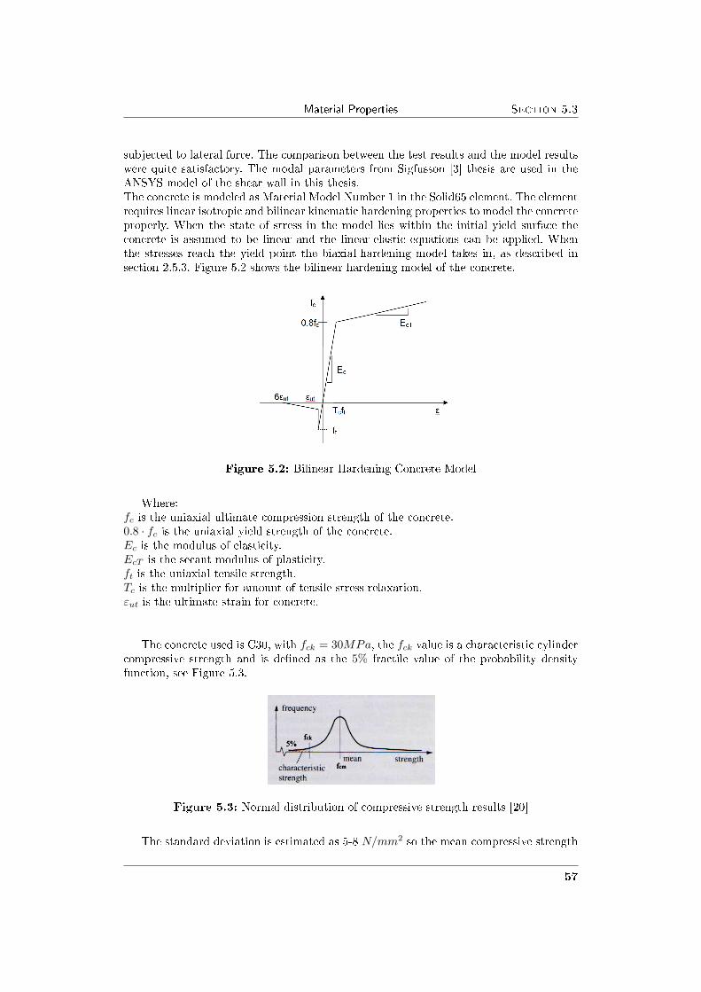
Material Properties Section 5.3
subjected to lateral force. The comparison between the test results and the model resultswere quite satisfactory. The modal parameters from Sigfusson [3] thesis are used in theANSYS model of the shear wall in this thesis.The concrete is modeled as Material Model Number 1 in the Solid65 element. The elementrequires linear isotropic and bilinear kinematic hardening properties to model the concreteproperly. When the state of stress in the model lies within the initial yield surface theconcrete is assumed to be linear and the linear-elastic equations can be applied. Whenthe stresses reach the yield point the biaxial-hardening model takes in, as described insection 2.5.3. Figure 5.2 shows the bilinear hardening model of the concrete.
Figure 5.2: Bilinear Hardening Concrete Model
Where:fc is the uniaxial ultimate compression strength of the concrete.0.8 · fc is the uniaxial yield strength of the concrete.Ec is the modulus of elasticity.EcT is the secant modulus of plasticity.ft is the uniaxial tensile strength.Tc is the multiplier for amount of tensile stress relaxation.εut is the ultimate strain for concrete.
The concrete used is C30, with fck = 30MPa, the fck value is a characteristic cylindercompressive strength and is de�ned as the 5% fractile value of the probability densityfunction, see Figure 5.3.
Figure 5.3: Normal distribution of compressive strength results [20]
The standard deviation is estimated as 5-8 N/mm2 so the mean compressive strength
57

Chapter 5 Nonlinear Pushover Analysis
for C30 concrete is roughly estimated to be:
fcm = 30 + (5− 8) = 35 to 38 MPa
It is decided to use the lower limit, fc=35MPaThe tensile strength is derived from the compression strength, fck and is estimated as:
fct = 0.3 · f2/3ck = 0.3 · 302/3 = 2.9MPa (5.3.1)
According to EC2 the modulus of elasticity of concrete depends not only on thestrength class of the concrete but also on the actual properties of the aggregates used:
Ec = 9.5 · (fck + 8)1/3 = 9.5 · (30 + 8)1/3 = 31656MPa (5.3.2)
The ultimate strain for concrete is 0.0035 indicating the crushing strain.
The bilinear kinematic material uses the von Mises failure criterion along with theWillam and Warnke model to de�ne the failure of the concrete, the Willam and Warnkemodel [4] is a �ve parameter model and as explained in section 2.5.3 it needs a total of�ve input strength parameters to de�ne the failure, the parameters are listed in Table 5.1.
Table 5.1: Input parameters for Willam and Warnke modelDescription LabelUltimate uniaxial tensile strength: ft
Ultimate uniaxial compressive strength: fc
Ultimate biaxial compressive strength: σah
Ultimate compressive strength for a state of biaxialcompression superimposed on hydrostatic stress state: f1
Ultimate compressive strength for a state of uniaxial compressionsuperimposed on hydrostatic stress state: f2
fcb = 1.2 · fc
f1 = 1.45 · fc
f2 = 1.725 · fc
The parameters needed to de�ne the material properties of the concrete are listed inTable 5.3. The typical shear transfer coe�cient is de�ned from zero to one, with zerorepresenting a smooth crack (complete loss of shear transfer) and one representing arough crack (no loss of shear transfer).
58

Material Properties Section 5.3
Table 5.2: Material parameters used the concreteNr Parameter C30 concrete1 Secant Modulus of elasticity [Ec] 31656 MPa2 Uniaxial ultimate compression strength [fc] 35 MPa3 Uniaxial tensile strength [ft] 2.9 MPa4 Secant modulus of plasticity [EΓ] 2 MPa5 Uniaxial yield strength for concrete 0.8 · fc = 29MPa6 Ultimate strain for concrete 3.5/pm7 Shear transfer coe�cient for an open crack [βt] 0.18 Shear transfer coe�cient for a closed crack [βc] 1.09 Multiplier for amount of tensile stress relaxation [Tc] 0.610 Poisson's ratio for concrete, elastic and cracked [ν] 0.211 Weight of concrete 24kN/m3
The reinforcement is modeled as Material Model Number 2 in the Solid65 element.The reinforcement used is fy = 500MPa steel, that is the yield strength is 500MPa. Thereinforcement material model is shown in Figure 5.4 and the parameters are shown inTable 5.3.
Figure 5.4: Steel Model
Table 5.3: Parameters for material number two, the steelNr Parameter reinforcement1 Poisson's ratio for steel 0.32 Modulus of elasticity for steel [Es] 210000 MPa3 Modulus of plasticity for steel [Ep] 1.035 MPa4 Yield point of steel [fy] 500 MPa5 Ultimate strain for steel [εu] 15±6 Weight of steel 77kN/m3
59

Chapter 5 Nonlinear Pushover Analysis
5.4 Analytical Nonlinear Model
The shear wall is modeled as a volume. All the nodes at the ground level are �xedand the displacement into the wall is prevented. To obtain good results from the Solid65element it is important to mesh the model properly. The analytical model of the meshedwall with its boundaries and applied loads is shown in Figure 5.5.
Figure 5.5: Modeling of the wall in Ansys
Table 5.4 shows the main characteristics of the �nite element model used in ANSYS.
Table 5.4: Main characteristics of the FEM model in ANSYSNr Finite element model ANSYS shear wall model1 Dimension of model 3D2 Total number of concrete elements 14923 Total number of reinforcement elements 14924 Cracking and crushing of elements YES5 Yielding of concrete and reinforcement YES6 Bond slip between steel and concrete NO7 Load step size 0.018 Iteration technique Newton-Rapson9 Convergence criteria Displacement norm, γ = 0.005
60

Analytical Results Section 5.5
Figure 5.6: Element numbers
5.5 Analytical Results
In the pushover analysis of the shear wall the lateral load was increased step-wise fromzero to twice as large as the calculated one to see how the wall behaves if the lateral loadexceeds the calculated design earthquake load, see section 3.3.2. For the double load thewall designed from SAP2000 reached numerical "failure" before the analyze was �nishedand therefore only one and a half of the calculated load was applied on that wall.
Figure 5.7 shows the load-de�ection curve or the capacity curve for the analysed walls.The force is normalized where one is the calculated design earthquake load. At the designearthquake load the ultimate top displacement is approximately 5.2 mm for the wall withminimum reinforcement according to EC2, 4.7 mm for the wall designed from SAP2000,4.1 mm for the wall designed from ETABS the minimum displacement, 3.8 mm, is for thewall designed according to the Stringer method.
61

Chapter 5 Nonlinear Pushover Analysis
0 1 2 3 4 5 60
0.1
0.2
0.3
0.4
0.5
0.6
0.7
0.8
0.9
1
deflection [mm]
Nor
mal
ized
Loa
d
ElasticEC2stringersap2000Etabs
Figure 5.7: Load de�ection curves for di�erent analysis
In Figure 5.8 the displacement has been normalized in the form of displacement ductil-ity. The yield de�ection is about 1 for all of the walls, see Figure 5.7, so the displacementductility has the same value as the displacement for each wall.
0 1 2 3 4 5 60
0.1
0.2
0.3
0.4
0.5
0.6
0.7
0.8
0.9
1
Displacement ductility
Nor
mal
ized
Loa
d
EC2stringersap2000Etabs
Figure 5.8: Ductility curves
62
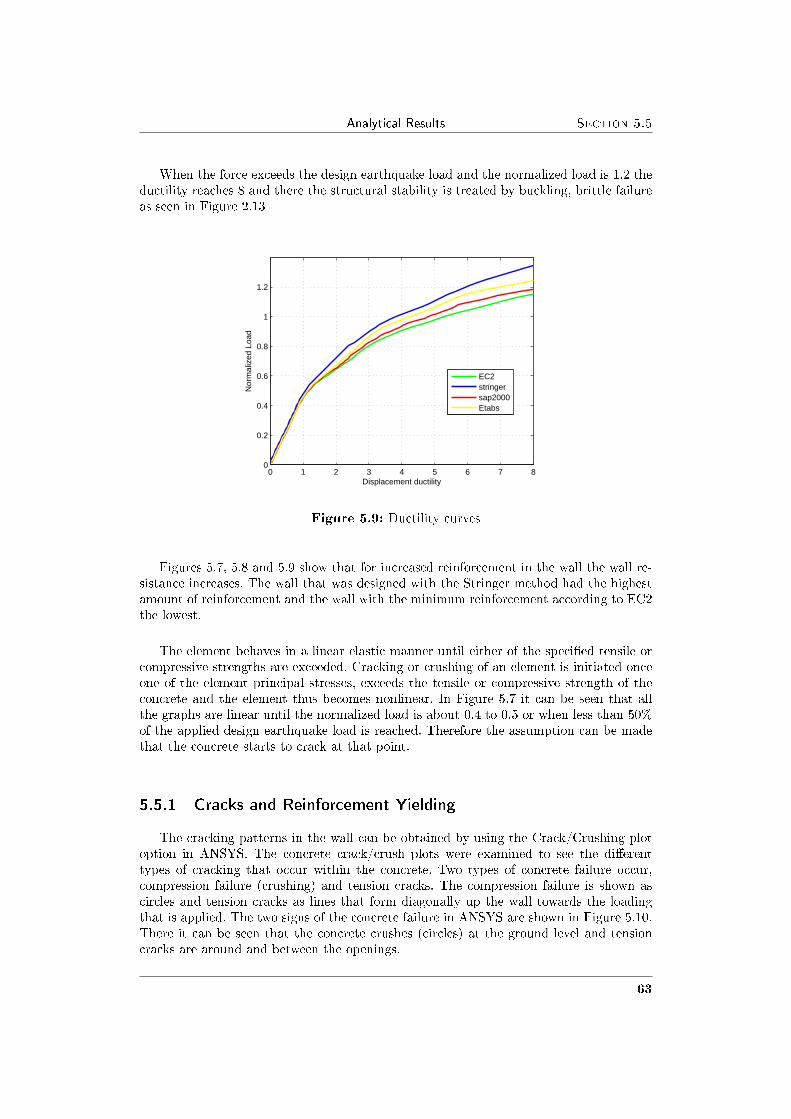
Analytical Results Section 5.5
When the force exceeds the design earthquake load and the normalized load is 1.2 theductility reaches 8 and there the structural stability is treated by buckling, brittle failureas seen in Figure 2.13
0 1 2 3 4 5 6 7 80
0.2
0.4
0.6
0.8
1
1.2
Displacement ductility
Nor
mal
ized
Loa
d
EC2stringersap2000Etabs
Figure 5.9: Ductility curves
Figures 5.7, 5.8 and 5.9 show that for increased reinforcement in the wall the wall re-sistance increases. The wall that was designed with the Stringer method had the highestamount of reinforcement and the wall with the minimum reinforcement according to EC2the lowest.
The element behaves in a linear elastic manner until either of the speci�ed tensile orcompressive strengths are exceeded. Cracking or crushing of an element is initiated onceone of the element principal stresses, exceeds the tensile or compressive strength of theconcrete and the element thus becomes nonlinear. In Figure 5.7 it can be seen that allthe graphs are linear until the normalized load is about 0.4 to 0.5 or when less than 50%of the applied design earthquake load is reached. Therefore the assumption can be madethat the concrete starts to crack at that point.
5.5.1 Cracks and Reinforcement Yielding
The cracking patterns in the wall can be obtained by using the Crack/Crushing plotoption in ANSYS. The concrete crack/crush plots were examined to see the di�erenttypes of cracking that occur within the concrete. Two types of concrete failure occur,compression failure (crushing) and tension cracks. The compression failure is shown ascircles and tension cracks as lines that form diagonally up the wall towards the loadingthat is applied. The two signs of the concrete failure in ANSYS are shown in Figure 5.10.There it can be seen that the concrete crushes (circles) at the ground level and tensioncracks are around and between the openings.
63

Chapter 5 Nonlinear Pushover Analysis
Figure 5.10: Cracking signs in ANSYS, NL=1
Figures 5.11 to 5.13 show the cracking in the shear wall for all the four di�erentreinforcement layouts. The crack pattern is very similar in all of the walls. The mostcritical area is around the middle opening of the second �oor, hereafter called the middleopening. The �rst tension cracking occurs in same elements for all of the walls. Theelements are numbered 778 and 670 and are located at the left upper corner and bottomright corner of the middle wall, see Figure 5.6. The concrete crushes at the ground levelof the wall.
Figure 5.11: Cracks at design earthquake load (NL = 1) for in the walldesigned with Stringer method
64

Analytical Results Section 5.5
Figure 5.12: Cracks at design earthquake load (NL = 1) in the wall de-signed from ETABS
Figure 5.13: Cracks at design earthquake load (NL = 1) in the wall de-signed from SAP2000
65

Chapter 5 Nonlinear Pushover Analysis
Figure 5.14: Cracks at design earthquake load (NL = 1) in the wall withminimum reinforcement, EC2
With increased load the tensile stresses get bigger than the tensile strength in theconcrete and its cracks and the tensile force is taken care of by the reinforcement. Thereforeit is interesting to see how the steel stress changes in the elements when the load isincreased. First the steel stress in element 787 is examined for all the walls. Element 787 islocated at the top left corner of the middle opening, see Figure 5.6. For the walls designedfrom the FE-analysis in ETABS and with the Stringer method, 4k16 is placed aroundthe opening while 2k16 is used when the design is based on the other two. Figure 5.15shows the steel stresses versus normalized load for the vertical reinforcement in element787. The stresses in the reinforcement start to increase when around 40% of the designearthquake load is reached for all the designed reinforcement layouts. It can be seen thatthe steel stresses in SAP2000 and EC2 increase faster than the other two. Despite thisless than 50% of the reinforcement strength is reached at the design earthquake load forthe 2k16 reinforcements.
66
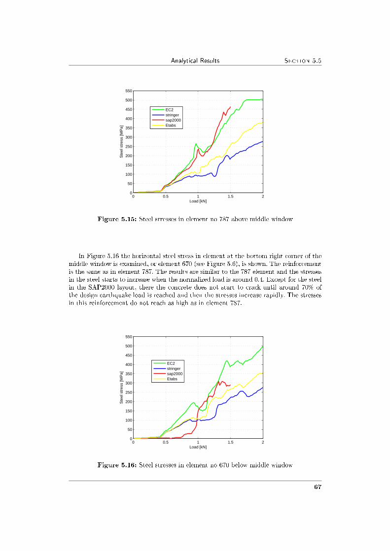
Analytical Results Section 5.5
0 0.5 1 1.5 20
50
100
150
200
250
300
350
400
450
500
550
Load [kN]
Ste
el s
tres
s [M
Pa]
EC2stringersap2000Etabs
Figure 5.15: Steel stresses in element no 787 above middle window
In Figure 5.16 the horizontal steel stress in element at the bottom right corner of themiddle window is examined, or element 670 (see Figure 5.6), is shown. The reinforcementis the same as in element 787. The results are similar to the 787 element and the stressesin the steel starts to increase when the normalized load is around 0.4. Except for the steelin the SAP2000 layout, there the concrete does not start to crack until around 70% ofthe design earthquake load is reached and then the stresses increase rapidly. The stressesin this reinforcement do not reach as high as in element 787.
0 0.5 1 1.5 20
50
100
150
200
250
300
350
400
450
500
550
Load [kN]
Ste
el s
tres
s [M
Pa]
EC2stringersap2000Etabs
Figure 5.16: Steel stresses in element no 670 below middle window
67

Chapter 5 Nonlinear Pushover Analysis
5.5.2 Calculations of Crack widthThe crush/crack plots of the walls show that the crack pattern in the walls are very
similar at the design earthquake load. A �gure of a crack does not tell all about the realdamage of the structures unless the widths of the cracks are known. An attempt was madeto calculate the width of the cracks by using information about the steel stresses fromthe ANSYS analysis and see if there is any di�erence between them in the four analysedwalls.In section 2.8.1 a method to calculate crack width based on EC2 was shown. The crackwidth can be found by the relation:
wk = β · srm · εsm (5.5.1)
srm is the average �nal crack spacing.εsm is the mean strain.β = 1.3, the width of the wall is less than 300 mm.εsm may be calculated from the relation:
εsm =σs
Es(1− β1β2(
σsr
σs)2) (5.5.2)
σs is the stress in the reinforcement and can be taken from ANSYS for each time step.σsr the stress in the tension when the �rst crack occurs, taken from ANSYS.β1 = 1, high bond bars.β2 = 0.5, earth quake load.The average �nal crack spacing for members subjected dominantly to �exure or tensioncan be calculated from the equation:
srm = 50 + 0.25k1k2φ/pr (5.5.3)
φ is the bar size in mm in the element.k1 = 0.8k2 = 0.5
The calculations were made in MATLAB and the crack width plotted as function ofthe normalized load.
In section 2.7 it was explained according to EC2 that the crack width should notexceed 0.3 mm to prevent corrosion of the reinforcement, which happens if the crackstarts to leak. From experience of Icelandic houses a crack need to be repaired if its widthis between 0.3 mm and 0.5 mm, but that is usually only necessary to improve the visualor a aesthetic view of the wall. Nevertheless the damaging impact on the concrete fromeach crack has to be evaluated individually. Crack 0.3 mm wide is visible at distance ofabout 2.0 m and it usually does not start to leak. For a crack of this size a light repair isusually enough where and surface treatment is enough were monosilan, siloxan or similarmaterial is applied on the concrete surface to conceal the projection of cracks. If the crackreaches 0.5 mm or more the damage starts to get more serious and more costly to repair.The concrete might start to leak and epoxy injection is necessary. The main purpose withthe repair is to prevent leaking, restore the original strength and sti�ness.
First element 787 is examined, see Figure 5.17 where the crack width is shown asfunction of the applied load. It can be seen that when the design earthquake load is
68

Analytical Results Section 5.5
reached the crack width for the wall designed from ETABS and Stringer method with4k16 in the element is under 0.3 mm but the crack width in the wall designed fromSAP2000 and minimum EC2 reinforcement with 2k16 is around 0.6 to 0.7 mm.The results are very similar for element 670 as seen in Figure 5.18.
0 0.5 1 1.5 20
0.1
0.2
0.3
0.4
0.5
0.6
0.7
0.8
0.9
1
1.1
1.2
1.3
1.4
1.5
Normalized Load
Des
ign
crac
k w
idth
[mm
]
EC2stringersap2000Etabs
Figure 5.17: Computed crack width in element 787
0 0.5 1 1.5 20
0.1
0.2
0.3
0.4
0.5
0.6
0.7
0.8
0.9
1
1.1
1.2
1.3
1.5
Normalized Load
Des
ign
crac
k w
idth
[mm
]
EC2stringersap2000Etabs
Figure 5.18: Computed crack width in element 670
From �gures 5.17 and 5.18 it is obvious that the reinforcement has great in�uenceon the crack width. The crack widt is smaller for higher reinforcement degree, i.e. 4k16than the lower degree 2k16. Therefore it is also interesting to look at an element werethe reinforcement area is the same for all of the four walls. Element 1026 is examined1026 which is between the windows on the third and the second �oor, see Figure 5.6.
69

Chapter 5 Nonlinear Pushover Analysis
The element is reinforced with k10c200. Even though the reinforcement is the same in allof the walls the results are similar as for the other two elements. At design earthquakeload the crack width is around 0.3 mm for the walls designed from ETABS and Stringermethod and is between 0.8 to 0.9 mm for the other two.
0 0.5 1 1.5 20
0.1
0.2
0.3
0.4
0.5
0.6
0.7
0.8
0.9
1
1.1
1.2
1.3
1.4
Normalized Load
Des
ign
crac
k w
idth
[mm
]
EC2stringersap2000Etabs
Figure 5.19: Design crack width in element 1026
70

Analytical Results Section 5.5
Next a look will be taken into the crack growth, it starts in element 670 at the rightbottom corner of the middle window and goes down to element 441. The crack growth inall the walls for the same elements are examined. It starts by looking at the wall designedwith the Stringer method. A close up �gure of the elements can be seen in Figure 5.20.
Figure 5.20: Cracks at middle window for Stringer
The concrete starts to crack in element 670 when the normalized load is 0.4 of thedesign load, in element 625 at 0.52 and the the last crack formed before the designearthquake load is reached is in element 441 when the normalized load is 0.9, but the crackopening is really small in the beginning and does not start to open until the normalizedload is around 1.5. In element 670 the reinforcement is 4k16 and 2k10c200 in the other�ve elements. The crack pattern can be seen in Figure 5.21, at design earthquake loadthe crack width is well below 0.3 mm at all places.
0 0.5 1 1.5 20
0.1
0.2
0.3
0.4
0.5
Normalized Load
Des
ign
crac
k w
idth
[mm
]
el. 670el. 625el. 579el. 533el. 487
Figure 5.21: Cracks width for Stringer
71

Chapter 5 Nonlinear Pushover Analysis
Now the same elements in the model designed with the FE-analysis in ETABS areexamined. The close up view of the cracks and can be seen in Figure 5.23. When the�gure is compared with Figure 5.20 it can be seen that the crack pattern is very similar.The reinforcement in element 670 is 4k16 and k10c200 in the other �ve.
Figure 5.22: Cracks at middle window for ETABS
The concrete starts to crack in element 670 when 40% of the design earthquake loadis reached. Cracks in the other elements start to develop shortly after the �rst crack andthe crack width grows rapidly in elements 625 to 487, where the reinforcement is twiceas low as in the elements for Stringer method. Despite this the crack width is under 0.3mm for all of the elements at the design earthquake load.
0 0.5 1 1.5 20
0.1
0.2
0.3
0.4
0.5
0.6
0.7
Normalized Load
Des
ign
crac
k w
idth
[mm
]
el. 670el. 625el. 579el. 533el. 487
Figure 5.23: Cracks width for ETABS
72
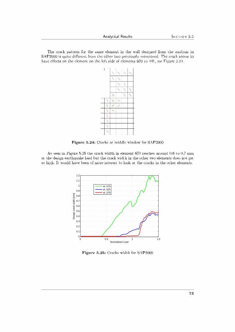
Analytical Results Section 5.5
The crack pattern for the same element in the wall designed from the analysis inSAP2000 is quite di�erent from the other two previously mentioned. The crack seems tohave e�ects on the element on the left side of elements 670 to 441, see Figure 5.24.
Figure 5.24: Cracks at middle window for SAP2000
As seen in Figure 5.25 the crack width in element 670 reaches around 0.6 to 0.7 mmat the design earthquake load but the crack width in the other two elements does not getso high. It would have been of more interest to look at the cracks in the other elements.
0 0.5 1 1.50
0.1
0.2
0.3
0.4
0.5
0.6
0.7
0.8
0.9
1
1.1
1.2
Normalized Load
Des
ign
crac
k w
idth
[mm
]
el. 670el. 625el. 579
Figure 5.25: Cracks width for SAP2000
73

Chapter 5 Nonlinear Pushover Analysis
Finally the same elements for the wall designed with minimum reinforcement accordingto EC2 are examined with 2k16 around the openings. It can be seen that there are slightlymore cracks seen on Figure 5.26 than in Figure 5.20 and 5.22.
Figure 5.26: Cracks at middle window for EC2
Cracking in element 670 starts when the normalized load is about 0.4 and the crackingin the other element follows quickly after and the growth of the crack width is fast. Atthe design earthquake load the width for elements 670, 625 and 579 has reached 0.3 mm,see Figure 5.27. At the design earthquake load the assumption can be made that a crackof length 75 cm and width of 0.3 mm or higher has been formed in the concrete belowthe opening because of the design earthquake load.
0 0.5 1 1.5 20
0.1
0.2
0.3
0.4
0.5
0.6
0.7
0.8
0.9
1
1.1
1.2
1.3
Normalized Load
Des
ign
crac
k w
idth
[mm
]
el. 670el. 625el. 579el. 533el. 487el. 441
Figure 5.27: Cracks width for EC2
74

Chapter 6
Summary and Conclusion
In the thesis a nonlinear pushover analysis of idealized three story concrete shear wallbuilding with di�erent seismic reinforcement design was presented. The building was as-sumed to be located in the South Iceland Seismic Zone where the characteristic peakground acceleration is 0.4g. This re�ects a design earthquake with 475 year return period.In the thesis only one wall of the building was studied. The design earthquake load wasde�ned by the lateral force method from Eurocode 8.
Three methods were used for the seismic design of the reinforcement in the shearwall. First, the Stringer method which is a lower bound method. Second, a design basedon linear elastic FE-analysis using the general purpose FE-program SAP2000. Third, adesign based again on linear elastic FE-analysis but now using the building specializedFE-program, ETABS. For comparison reinforcement based on the minimum requirementaccording to EC2 was also studied. The reinforcement from the Stinger Method and theone based on the ETABS analysis gave very similar reinforcement layouts. These methodsgave more boundary reinforcement, i.e. reinforcement around openings than the other twomethods.
A nonlinear �nite element model was created in ANSYS for the four reinforcementlayouts to carry out a pushover analysis of the di�erent shear wall design. The lateral loadwas stepwise increased from zero to twice the design earthquake load. With the model itwas possible to get information about deformations, initial cracks, tensile cracks, crushing,steel stresses and plastic deformations. However, the model gave no information aboutcrack widths which are crucial in order to estimate damage. For that reason an attemptwas made to evaluate crack widths as a function of load with method from Eurocode 2.In this method the steel stresses is the most important factor and it is important that thestresses in the reinforcement does not get too high.
When the response results of the di�erent walls were compared it turned out thatthe reinforcement layouts calculated from the Stringer Method and ETABS analysis gavevery similar results. On the other hand the reinforcement layouts from SAP2000 and theminimum reinforcement according to EC2 were similar. The design based on ETABS andthe Stringer method gave better results, i.e. less crack widths and overall less damagefor the same load level. The results clearly indicate that di�erent reinforcement layoutsa�ect the response of the wall. At the most critical points in the wall the two layoutsfrom ETABS and Stringer method were under acceptable crack widths, 0,3 mm, whensubjected to design earthquake load, while the minimum reinforcement according to EC2
75
Chapter 6 Summary and Conclusion
and the layout from SAP2000 gave far higher crack widths, or up to 0.9 mm. The di�er-ence in crack width is mainly due to the boundary reinforcement. It should be underlinedthat the technique used to average the stresses from the linear elastic FE-analysis withSAP2000 in the boundary areas of the wall greatly a�ects the amount of boundary rein-forcement. In this thesis the FE-stresses were averaged over 0.5 m wide strip which seemsto be to wide strip. This is something that should be studied in more details.
The crack widths calculated by using the information from ANSYS seem to be promis-ing and useful when designing and analysing structures in seismic zones. However, theresults from the nonlinear static procedure must be taken with caution, and the resultsneed to be veri�ed by experimental data.
In this thesis only one shear wall was studied and only one material set, i.e. concreteand steel type. In the future more types of shear walls and material sets could be studiedas well as laboratory tests to backup the numerical results. Finally, it could be veryinformative and valuable to back calculate reported damage during the South Icelandearthquakes of June 2000 in order to learn from them.
76

Appendix A
MATLAB script for Design Response spectra
%----------------------------------------------------------------function Sdh = hordesignSd(ag,T,TB,TC,TD,nu,q,beta,S)%----------------------------------------------------------------% INPUT:% ag: Design acceleration% T: Vibration period of a linear% single-degre-of-freedom system.% TB, TC: The limits of the constant spectral% acceleration branch% TD: The value defining the beginning of the% constant displacement response range of% the spectrum.% nu: Damping correction factor% q: Behaviour factor% beta: Lower bound factor% S: Soil factor%% OUTPUT: Sd : the horizontal design response spectrum%----------------------------------------------------------------
% Respons calculation, Sdhif T>=0 & T<=TB
Sdh = ag*S*(2/3+(T/TB)*(2.5/q-2/3));elseif T>TB & T<=TC
Sdh = ag*S*2.5/q;elseif T>TC & T<=TD
Sdh = max(ag*S*(2.5/q)*(TC/T), beta*ag);else
Sdh = max(ag*S*2.5/q*(TC*TD/T^2), beta*ag);end
%===================================================================% Structural response%---------------------------------------------------------------
clear all close all format short g format compact
77

Appendix A MATLAB script for Design Response spectra
% Parametersgamma1 = 1; % important class II EC8 Table 4.3g=9.81;ag = 0.4*g*gamma1; % design ground accelerationavg = 0.9*ag; % vertical design ground accelerationq = 2.34; % the behaviour factorS = 1; % soil factor, EC8 table 3.2 Type Dbeta = 0.2; % lower bound factor for design spectrumzeta = 0.05; % assumend damping ratio of buildingeta = max(sqrt(10/(5+zeta*100)),0.55) % correction factor for damping
% ------------ Respons spectrum ------------------------------------
% Values from EC8 table 3.2TBh = 0.15; % limits of the constant spectral
% acceleration branchTCh = 0.40; % limits of the constant spectral
% acceleration branchTDh = 2.00; % value defining the beginning of
% the constant displacement response of% the spectrum
n=0.01; % time step for spectrumT=0:n:4; % Evaluation spectra for T = [0;4]
% Horizontal design response spectrumSdh = zeros(1,size(T,1)); for i = 1:size(T,2)
Sdh(i) = hordesignSd(ag,T(i),TBh,TCh,TDh,eta,q,beta,S);end
% ------------Plot of respons spetrum -------------------------------figure(1) A=[Sdh/ag]; plot(T,A)
axis([0 4 0 1.3])
legend('Horizontal design') title(['The response spectrum for \zeta= ', num2str(zeta)]); xlabel('T') ylabel('{S_{dh}/a_g}') hold offprint -dmeta response.eps % dump encapsulated EMF file
78

Appendix B
Calculations for Stringer method
close all clear all format short
A=200*[4*1000 3*2500 0 0 0 0 0 0 0 0 0 0 0 0 0 0 0 0;0 0 4*1000 0 0 0 0 0 0 0 0 0 0 0 0 0 0 0;0 0 0 4*1000 3*2500 0 0 0 0 0 0 0 0 0 0 0 0 0;0 0 0 0 0 4*1000 3*2500 0 0 0 0 0 0 0 0 0 0 0;0 0 0 0 0 0 0 4*1000 0 0 0 0 0 0 0 0 0 0;0 0 0 0 0 0 0 0 4*1000 3*2500 0 0 0 0 0 0 0 0;0 0 0 0 0 0 0 0 0 0 4*1000 3*2500 0 0 0 0 0 0;0 0 0 0 0 0 0 0 0 0 0 0 2*1000 0 0 1750 0 1750;0 0 0 0 0 0 0 0 0 0 0 0 0 2*1000 2*2500 0 1750 1750;700 0 1200 1100 0 700 0 1200 1100 0 700 0 1200 1100 0 0 0 0;0 700 0 0 1100 0 700 0 0 1100 0 700 0 0 1100 0 0 0;700 0 1200 1100 0 700 0 1200 1100 0 700 0 1200 1100 0 0 0 0;0 700 0 0 1100 0 700 0 0 1100 0 700 0 0 1100 0 0 0;700 0 1200 1100 0 700 0 1200 1100 0 700 0 0 0 0 1200 1100 0;0 700 0 0 1100 0 700 0 0 1100 0 700 0 0 0 1200 1100 0;0 700 0 0 1100 0 700 0 0 1100 0 700 0 0 0 0 0 0;0 700 0 0 1100 0 700 0 0 1100 0 700 0 0 0 0 0 2300;700 0 1200 1100 0 700 0 1200 1100 0 700 0 0 0 0 0 0 2300];
b= [-570000;-570000-570000-1183000-1183000-1183000-1490000-1490000-1490000-449000-819000-994000-1092000-994000-819000
79
Appendix B Calculations for Stringer method
-819000-819000-449000];
x=pinv(A)*b
bnalgun =A*x;
skekkja1=(bnalgun./b-1)*100
%-------------------------------------------------------------------------%Horizontal stringerforces%-------------------------------------------------------------------------
%PLOTS%plot settingsset(0,'DefaultAxesFontName','Times')set(0,'DefaultAxesFontAngle','Normal')set(0,'DefaultAxesFontSize',10) set(0,'DefaultTextFontName','Times')set(0,'DefaultTextFontAngle','Oblique')set(0,'DefaultTextFontSize',10)
t=200;
F1x=-570000; F2x=F1x-1000*x(1)*t; F3x=F2x-2500*x(2)*t;F4x=F3x-1000*x(1)*t; F5x=F4x-2500*x(2)*t; F6x=F5x-1000*x(1)*t;F7x=F6x-2500*x(2)*t; F8x=F7x-1000*x(1)*t;
figure(1) subplot(3,1,1) plot([1 2 3 4 5 6 7 8],[F1x F2x F3x F4x F5xF6x F7x F8x]/1000) xlabel('stringerline no 1') grid ontitle('Horizontal stringer forces')
F9x=0; F10x=1000*t*(x(1)-x(3)); F11x=F10x+x(2)*2500*t;F12x=F11x+t*1000*(x(1)-x(3)); F13x=F12x+x(2)*2500*t;F14x=F13x+(x(1)-x(3))*1000*t; F15x=F14x+x(2)*2500*t;F16x=F15x+(x(1)-x(3))*1000*200; subplot(3,1,2) plot([9 10 11 12 1314 15 16],[F9x F10x F11x F12x F13x F14x F15x F16x]/1000)
Ylabel('Stringerforce [kN]') xlabel('stringerline no 2') grid on
F17x=0; F18x=(x(3)-x(4))*1000*t; F19x=F18x-x(5)*2500*t;F20x=F19x+(x(3)-x(4))*1000*t; F21x=F20x-x(5)*2500*t;F22x=F21x+(x(3)-x(4))*1000*t; F23x=F22x-x(5)*2500*t;F24x=F23x+(x(3)-x(4))*1000*t;
subplot(3,1,3) plot([17 18 19 20 21 22 23 24],[F17x F18x F19x F20x
80

Section B.0
F21x F22x F23x F24x]/1000)
xlabel('stringerline no 3') grid on print -dwinc horstringforce1.eps
figure(2)
F25x=-613000; F26x=F25x+1000*(x(4)-x(6))*t;F27x=F26x+2500*(x(5)-x(7))*t; F28x=F27x+1000*(x(4)-x(6))*t;F29x=F28x+2500*(x(5)-x(7))*t; F30x=F29x+1000*(x(4)-x(6))*t;F31x=F30x+2500*(x(5)-x(7))*t; F32x=F31x+1000*(x(4)-x(6))*t;
subplot(3,1,1)
plot([25 26 27 28 29 30 31 32],[F25x F26x F27x F28x F29x F30x F31xF32x]/1000)
xlabel('stringerline no 4') title('Horizontal stringer forces') gridon
F33x=0; F34x=(x(6)-x(8))*1000*t; F35x=F34x+x(7)*2500*t;F36x=F35x+(x(6)-x(8))*1000*t; F37x=F36x+x(7)*2500*t;F38x=F37x+(x(6)-x(8))*1000*t; F39x=F38x+x(7)*2500*t;F40x=F39x+(x(6)-x(8))*1000*t;
subplot(3,1,2) plot([33 34 35 36 37 38 39 40],[F33x F34x F35x F36xF37x F38x F39x F40x]/1000)
Ylabel('Stringerforce [kN]') xlabel('stringerline no 5') grid on
F41x=0; F42x=(x(8)-x(9))*1000*t; F43x=F42x-x(10)*2500*t;F44x=F43x+(x(8)-x(9))*1000*t; F45x=F44x-x(10)*2500*t;F46x=F45x+(x(8)-x(9))*1000*t; F47x=F46x-x(10)*2500*t;F48x=F47x+(x(8)-x(9))*1000*t;
subplot(3,1,3) plot([41 42 43 44 45 46 47 48],[F41x F42x F43x F44xF45x F46x F47x F48x]/1000)
xlabel('stringerline no 6') grid on print -dwinc horstringforce2.epsfigure(3)
F49x=-307000; F50x= F49x+1000*(x(9)-x(11))*t;F51x=F50x+2500*(x(10)-x(12))*t; F52x=F51x+1000*(x(9)-x(11))*t;F53x=F52x+2500*(x(10)-x(12))*t; F54x=F53x+1000*(x(9)-x(11))*t;F55x=F54x+2500*(x(10)-x(12))*t; F56x=F55x+1000*(x(9)-x(11))*t;
subplot(4,1,1)
plot([49 50 51 52 53 54 55 56],[F49x F50x F51x F52x F53x F54x F55xF56x]/1000) title('Horizontal stringer forces') xlabel('stringerline
81

Appendix B Calculations for Stringer method
no 7') grid on
F57x=0; F58x=(x(11)-x(13))*1000*t; F59x=F58x+x(12)*2500*t;F60x=F59x+(x(11)-x(13))*1000*t; F61x=F60x+x(12)*2500*t;F62x=F61x+(x(11)-x(16))*1000*t; F63x=F62x+(x(12)-x(16))*750*t;F64x=F63x+x(12)*1000*t; F65x=F64x+(x(12)-x(16))*750*t;F66x=F65x+(x(11)-x(18))*1000*t;
subplot(4,1,2) plot([57 58 59 60 61 62 63 64 65 66],[F57x F58x F59xF60x F61x F62x F63x F64x F65x F66x]/1000)
Ylabel('Stringerforce [kN]') xlabel('stringerline no 8') grid on
F67x=0; F68x=(x(13)-x(14))*1000*t; F69x=F68x-x(15)*2500*t;F70x=F69x+(x(13)-x(14))*1000*t; F71x=F70x-x(15)*2500*t;F72x=F71x+(x(16)-x(17))*1000*t; F73x=F72x+(x(16)-x(17))*750*t;F74x=F73x; F75x=F74x+(x(18)-x(18))*750*t;F76x=F75x+(x(18)-x(18))*1000*t;
subplot(4,1,3) plot([67 68 69 70 71 72 73 74 75 76],[F67x F68x F69xF70x F71x F72x F73x F74x F75x F76x]/1000)
xlabel('stringerline no 9') grid on
F77x=0; F78x=x(14)*1000*t; F79x=F78x+x(15)*2500*t;F80x=F79x+x(14)*1000*t; F81x=F80x+x(15)*2500*t;F82x=F81x+x(17)*1000*t; F83x=F82x+x(17)*750*t; F84x=F83x;F85x=F84x+x(18)*750*t; F86x=F85x+x(18)*1000*t;
subplot(4,1,4) plot([77 78 79 80 81 82 83 84 85 86],[F77x F78x F79xF80x F81x F82x F83x F84x F85x F86x]/1000) xlabel('stringerline no10') grid on print -dwinc horstringforce3.eps%-------------------------------------------------------------------------%Vertical stringerforces%-------------------------------------------------------------------------
F77y=449000; F67y=F77y+x(14)*1100*t; F57y=F67y+x(13)*1200*t;F49y=F57y+x(11)*700*t; F41y=F49y+x(9)*1100*t; F33y=F41y+x(8)*1200*t;F25y=F33y+x(6)*700*t; F17y=F25y+x(4)*1100*t; F9y=F17y+x(3)*1200*t;F1y=F9y+x(1)*1000*t;
figure(4)
set(gca,'YDir','reverse') subplot(1,4,1) plot([F77y F67y F57y F49yF41y F33y F25y F17y F9y F1y]/1000, [77 67 57 49 41 33 25 17 9 1])set(gca,'YDir','reverse') set(gca,'ytick',[1 9 17 25 33 41 49 57 67
82

Section B.0
77]) axis([-1000 1000 1 77]) ylabel('stringerline no 11')
grid on
F78y=370000; F68y=F78y+(x(15)-x(14))*1100*t; F58y=F68y-x(13)*1200*t;F50y=F58y+(x(12)-x(11))*700*t; F42y=F50y+(x(10)-x(9))*1100*t;F34y=F42y-x(8)*1200*t; F26y=F34y+(x(7)-x(6))*700*t;F18y=F26y+(x(5)-x(4))*1100*t; F10y=F18y-x(3)*1200*t;F2y=F10y+(x(1)-x(2))*1200*t;
subplot(1,4,2) plot([F2y F10y F18y F26y F34y F42y F50y F58y F68yF78y]/1000, [2 10 18 26 34 42 50 58 68 78])set(gca,'YDir','reverse') set(gca,'ytick',[2 10 18 26 34 42 50 58 6878]) axis([-500 600 2 78]) title('Vertical stringer forces')ylabel('stringerline no 12') xlabel('Stringerforce [kN]') grid on
F79y=175000; F69y=F79y+(x(14)-x(15))*1100*t; F59y=F69y+x(13)*1200*t;F51y=F59y+(x(11)-x(12))*700*t; F43y=F51y+(x(9)-x(10))*1100*t;F35y=F43y+x(8)*1200*t; F27y=F35y+(x(6)-x(7))*700*t;F19y=F27y+(x(4)-x(5))*1100*t; F11y=F19y+x(3)*1200*t;F3y=F11y+(x(1)-x(2))*700*t;
subplot(1,4,3) plot([F3y F11y F19y F27y F35y F43y F51y F59y F69yF79y]/1000, [3 11 19 27 35 43 51 59 69 79])set(gca,'YDir','reverse') set(gca,'ytick',[3 11 19 27 35 43 51 59 6979]) axis([0 1200 3 78]) ylabel('stringerline no 13') grid on
F80y=98000; F70y=F80y+(x(15)-x(14))*1100*t; F60y=F70y-x(13)*1200*t;F52y=F60y+(x(12)-x(11))*700*t; F44y=F52y+(x(10)-x(9))*1100*t;F36y=F44y-x(8)*1200*t; F28y=F36y+(x(7)-x(6))*700*t;F20y=F28y+(x(5)-x(4))*1100*t; F12y=F28y-x(3)*1200*t;F4y=F12y+(x(2)-x(1))*700*t;
subplot(1,4,4) plot([F4y F12y F20y F28y F36y F44y F52y F60y F70yF80y]/1000,[4 12 20 28 36 44 52 60 70 80]) set(gca,'YDir','reverse')set(gca,'ytick',[4 12 20 28 36 44 52 60 70 80]) axis([-700 500 480]) ylabel('stringerline no 14') grid on print -dwincverstringforce1.eps
F81y=-98000; F71y=F81y+(x(15)-x(15))*1100*t; F61y=F71y+x(16)*1200*t;F53y=F61y+(x(11)-x(12))*700*t; F45y=F53y+(x(9)-x(10))*1100*t;F37y=F45y+x(8)*1200*t; F29y=F37y+(x(6)-x(7))*700*t;F21y=F29y+(x(4)-x(5))*1100*t; F13y=F21y+x(3)*1200*t;F5y=F13y+(x(1)-x(2))*700*t;
83
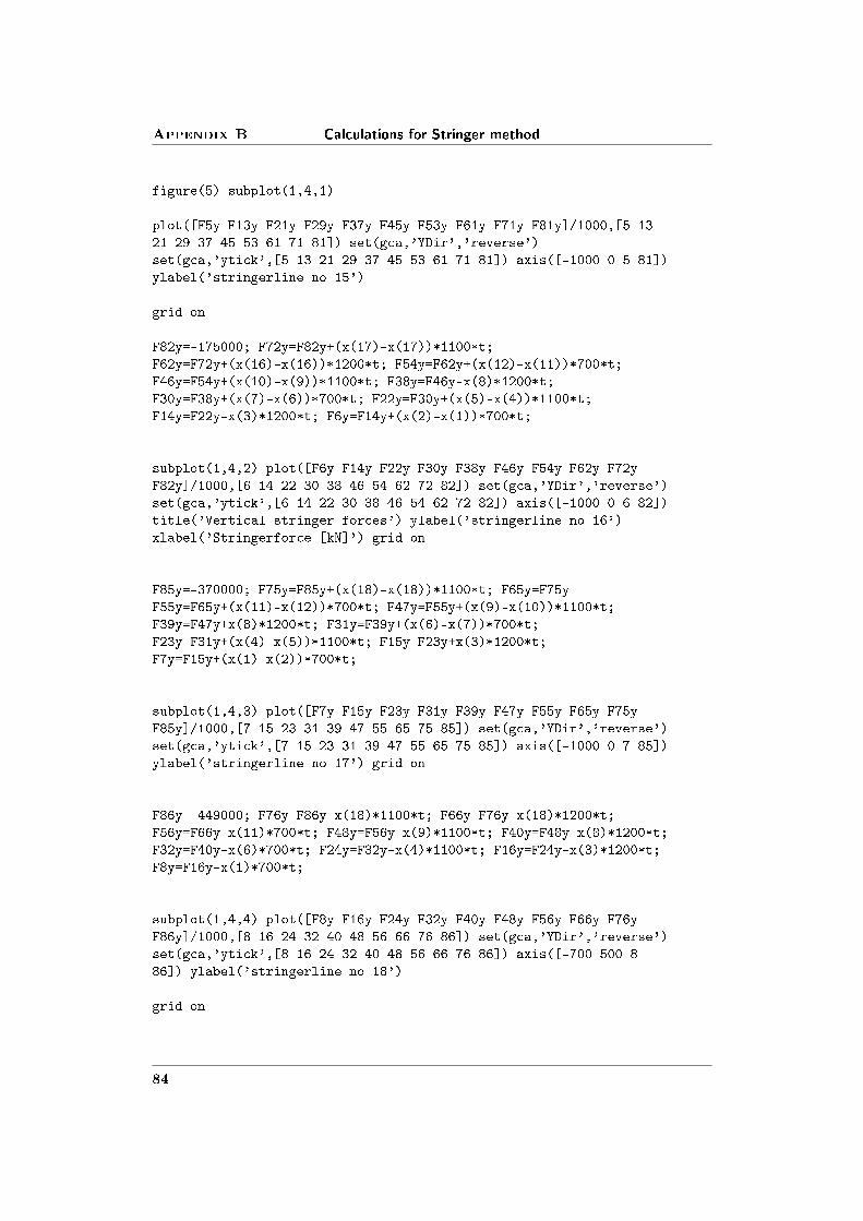
Appendix B Calculations for Stringer method
figure(5) subplot(1,4,1)
plot([F5y F13y F21y F29y F37y F45y F53y F61y F71y F81y]/1000,[5 1321 29 37 45 53 61 71 81]) set(gca,'YDir','reverse')set(gca,'ytick',[5 13 21 29 37 45 53 61 71 81]) axis([-1000 0 5 81])ylabel('stringerline no 15')
grid on
F82y=-175000; F72y=F82y+(x(17)-x(17))*1100*t;F62y=F72y+(x(16)-x(16))*1200*t; F54y=F62y+(x(12)-x(11))*700*t;F46y=F54y+(x(10)-x(9))*1100*t; F38y=F46y-x(8)*1200*t;F30y=F38y+(x(7)-x(6))*700*t; F22y=F30y+(x(5)-x(4))*1100*t;F14y=F22y-x(3)*1200*t; F6y=F14y+(x(2)-x(1))*700*t;
subplot(1,4,2) plot([F6y F14y F22y F30y F38y F46y F54y F62y F72yF82y]/1000,[6 14 22 30 38 46 54 62 72 82]) set(gca,'YDir','reverse')set(gca,'ytick',[6 14 22 30 38 46 54 62 72 82]) axis([-1000 0 6 82])title('Vertical stringer forces') ylabel('stringerline no 16')xlabel('Stringerforce [kN]') grid on
F85y=-370000; F75y=F85y+(x(18)-x(18))*1100*t; F65y=F75yF55y=F65y+(x(11)-x(12))*700*t; F47y=F55y+(x(9)-x(10))*1100*t;F39y=F47y+x(8)*1200*t; F31y=F39y+(x(6)-x(7))*700*t;F23y=F31y+(x(4)-x(5))*1100*t; F15y=F23y+x(3)*1200*t;F7y=F15y+(x(1)-x(2))*700*t;
subplot(1,4,3) plot([F7y F15y F23y F31y F39y F47y F55y F65y F75yF85y]/1000,[7 15 23 31 39 47 55 65 75 85]) set(gca,'YDir','reverse')set(gca,'ytick',[7 15 23 31 39 47 55 65 75 85]) axis([-1000 0 7 85])ylabel('stringerline no 17') grid on
F86y=-449000; F76y=F86y-x(18)*1100*t; F66y=F76y-x(18)*1200*t;F56y=F66y-x(11)*700*t; F48y=F56y-x(9)*1100*t; F40y=F48y-x(8)*1200*t;F32y=F40y-x(6)*700*t; F24y=F32y-x(4)*1100*t; F16y=F24y-x(3)*1200*t;F8y=F16y-x(1)*700*t;
subplot(1,4,4) plot([F8y F16y F24y F32y F40y F48y F56y F66y F76yF86y]/1000,[8 16 24 32 40 48 56 66 76 86]) set(gca,'YDir','reverse')set(gca,'ytick',[8 16 24 32 40 48 56 66 76 86]) axis([-700 500 886]) ylabel('stringerline no 18')
grid on
84

Section B.0
print -dwinc verstringforce2.eps%-------------------------------------------------------------------------%Reinforcement%-------------------------------------------------------------------------fcd=20 %MPafyd=435 %MPa%-------------------------------------------------------------------------%Reinforcement horizontal%-------------------------------------------------------------------------
%STRINGER 1%Tension reinforcementFhor1=[F1x F2x F3x F4x F5x F6x F7x F8x]/1000;
%The concrete can take up compressionforce:C1=0.2*800*t*0.5*fcd*0.001; for i=1:length(Fhor1); if Fhor1(i)>0 ;
Axten1(i)=Fhor1(i)*1000/fyd;else Axten1(i)=0; end end
Axten1
%Compression reinforcement
Fcom1=Fhor1+C1; for j=1:length(Fcom1) if Fcom1(j)<0;Axcom1(j)=(Fcom1(j))*1000/fyd;
else Axcom1(j)=0; end end
Axcom1
%STRINGER 2
%Tension reinforcementFhor2=[F9x F10x F11x F12x F13x F14x F15x F16x]/1000;
%The concrete can take up compressionforce:C2=0.2*800*t*0.5*fcd*0.001; for i=1:length(Fhor2); if Fhor2(i)>0 ;
Axten2(i)=Fhor2(i)*1000/fyd;else Axten2(i)=0; end end
Axten2
%Compression reinforcement
Fcom2=Fhor2+C2; for j=1:length(Fcom2) if Fcom2(j)<0;Axcom2(j)=(F1com(j))*1000/fyd;
else Axcom2(j)=0; end end
85

Appendix B Calculations for Stringer method
Axcom2
%STRINGER 3%Tension reinforcementFhor3=[F17x F18x F19x F20x F21x F22x F23x F24x]/1000;
%The concrete can take up compressionforce:C3=0.2*1100*t*0.5*fcd*0.001; for i=1:length(Fhor3); if Fhor3(i)>0 ;
Axten3(i)=Fhor3(i)*1000/fyd;else Axten3(i)=0; end end
Axten3
%Compression reinforcement
Fcom3=Fhor3+C3; for j=1:length(Fcom3) if Fcom3(j)<0;Axcom3(j)=(Fcom3(j))*1000/fyd;
else Axcom3(j)=0; end end
Axcom3
%STRINGER 4%Tension reinforcementFhor4=[F25x F26x F27x F28x F29x F30x F31x F32x]/1000;
%The concrete can take up compressionforce:C4=0.2*800*t*0.5*fcd*0.001; for i=1:length(Fhor4); if Fhor4(i)>0 ;
Axten4(i)=Fhor4(i)*1000/fyd;else Axten4(i)=0; end end
Axten4
%Compression reinforcement
Fcom4=Fhor4+C4; for j=1:length(Fcom4) if Fcom4(j)<0;Axcom4(j)=(Fcom4(j))*1000/fyd;
else Axcom4(j)=0; end end
Axcom4
%STRINGER 5%Tension reinforcementFhor5=[F33x F34x F35x F36x F37x F38x F39x F40x]/1000;
%The concrete can take up compressionforce:C5=0.2*800*t*0.5*fcd*0.001; for i=1:length(Fhor5); if Fhor5(i)>0 ;
86

Section B.0
Axten5(i)=Fhor5(i)*1000/fyd;else Axten5(i)=0; end end
Axten5
%Compression reinforcement
Fcom5=Fhor5+C5; for j=1:length(Fcom4) if Fcom5(j)<0;Axcom5(j)=(Fcom5(j))*1000/fyd;
else Axcom5(j)=0; end end
Axcom5
%STRINGER 6%Tension reinforcementFhor6=[F41x F42x F43x F44x F45x F46x F47x F48x]/1000;
%The concrete can take up compressionforce:C6=0.2*1100*t*0.5*fcd*0.001; for i=1:length(Fhor6); if Fhor6(i)>0 ;
Axten6(i)=Fhor6(i)*1000/fyd;else Axten6(i)=0; end end
Axten6
%Compression reinforcement
Fcom6=Fhor6+C6; for j=1:length(Fcom6) if Fcom6(j)<0;Axcom6(j)=(Fcom6(j))*1000/fyd;
else Axcom6(j)=0; end end
Axcom6
%STRINGER 7%Tension reinforcementFhor7=[F49x F50x F51x F52x F53x F54x F55x F56x]/1000;
%The concrete can take up compressionforce:C7=0.2*800*t*0.5*fcd*0.001; for i=1:length(Fhor7); if Fhor7(i)>0 ;
Axten7(i)=Fhor7(i)*1000/fyd;else Axten7(i)=0; end end
Axten7
%Compression reinforcement
Fcom7=Fhor7+C7; for j=1:length(Fcom7) if Fcom7(j)<0;Axcom7(j)=(Fcom7(j))*1000/fyd;
87

Appendix B Calculations for Stringer method
else Axcom7(j)=0; end end
Axcom7
%STRINGER 8%Tension reinforcementFhor8=[F57x F58x F59x F60x F61x F62x F63x F64x F65x F66x]/1000;
%The concrete can take up compressionforce:C8=0.2*800*t*0.5*fcd*0.001; for i=1:length(Fhor8); if Fhor8(i)>0 ;
Axten8(i)=Fhor8(i)*1000/fyd;else Axten8(i)=0; end end
Axten8
%Compression reinforcement
Fcom8=Fhor8+C8; for j=1:length(Fcom8) if Fcom8(j)<0;Axcom8(j)=(Fcom8(j))*1000/fyd;
else Axcom8(j)=0; end end
Axcom8
%STRINGER 9%Tension reinforcementFhor9=[F67x F68x F69x F70x F71x F72x F73x F74x F75x F76x]/1000;
%The concrete can take up compressionforce:C9=0.2*1100*t*0.5*fcd*0.001; for i=1:length(Fhor9); if Fhor9(i)>0 ;
Axten9(i)=Fhor9(i)*1000/fyd;else Axten9(i)=0; end end
Axten9
%Compression reinforcement
Fcom9=Fhor9+C9; for j=1:length(Fcom9) if Fcom9(j)<0;Axcom9(j)=(Fcom9(j))*1000/fyd;
else Axcom9(j)=0; end end
Axcom9
%STRINGER 10%Tension reinforcementFhor10=[F77x F78x F79x F80x F81x F82x F83x F84x F85x F86x]/1000;
88

Section B.0
%The concrete can take up compressionforce:C10=0.2*1100*t*0.5*fcd*0.001; for i=1:length(Fhor10); if Fhor10(i)>0;
Axten10(i)=Fhor10(i)*1000/fyd;else Axten10(i)=0; end end
Axten10
%Compression reinforcement
Fcom10=Fhor10+C10; for j=1:length(Fcom10) if Fcom10(j)<0;Axcom10(j)=(Fcom10(j))*1000/fyd;
else Axcom10(j)=0; end end
Axcom10%-------------------------------------------------------------------------%Vertical reinforcement%-------------------------------------------------------------------------%STRINGER 11%Tension reinforcementFver1=[F1y F9y F17y F25y F33y F41y F49y F57y F67y F77y]/1000;
%The concrete can take up compressionforce:C1y=0.2*1000*t*0.5*fcd*0.001;
%Tension reinforcementfor i=1:length(Fver1); if Fver1(i)>0 ;
Ayten1(i)=Fver1(i)*1000/fyd;else Ayten1(i)=0; end end
Ayten1
%Compression reinforcement
Fcom1y=Fver1+C1y; for j=1:length(Fcom1y) if Fcom1y(j)<0;Aycom1(j)=(Fcom1y(j))*1000/fyd;
else Aycom1(j)=0; end end
Aycom1
%STRINGER 12%Tension reinforcementFver2=[F2y F10y F18y F26y F34y F42y F50y F58y F68y F78y]/1000;
%The concrete can take up compressionforce:C2y=0.2*1000*t*0.5*fcd*0.001;
89

Appendix B Calculations for Stringer method
%Tension reinforcementfor i=1:length(Fver2); if Fver2(i)>0 ;
Ayten2(i)=Fver2(i)*1000/fyd;else Ayten2(i)=0; end end
Ayten2
%Compression reinforcement
Fcom2y=Fver2+C2y; for j=1:length(Fcom2y) if Fcom2y(j)<0;Aycom2(j)=(Fcom2y(j))*1000/fyd;
else Aycom2(j)=0; end end
Aycom2
%STRINGER 12%Tension reinforcementFver3=[F3y F11y F19y F27y F35y F43y F51y F59y F69y F79y]/1000;
%The concrete can take up compressionforce:C3y=0.2*1000*t*0.5*fcd*0.001;
%Tension reinforcementfor i=1:length(Fver3); if Fver3(i)>0 ;
Ayten3(i)=Fver3(i)*1000/fyd;else Ayten3(i)=0; end end
Ayten3
%Compression reinforcement
Fcom3y=Fver3+C3y; for j=1:length(Fcom3y) if Fcom3y(j)<0;Aycom3(j)=(Fcom3y(j))*1000/fyd;
else Aycom3(j)=0; end end
Aycom3
%STRINGER 14%Tension reinforcementFver4=[F4y F12y F20y F28y F36y F44y F52y F60y F70y F80y]/1000;
%The concrete can take up compressionforce:C4y=0.2*1000*t*0.5*fcd*0.001;
%Tension reinforcementfor i=1:length(Fver4); if Fver4(i)>0 ;
Ayten4(i)=Fver4(i)*1000/fyd;
90

Section B.0
else Ayten4(i)=0; end end
Ayten4
%Compression reinforcement
Fcom4y=Fver4+C4y; for j=1:length(Fcom4y) if Fcom4y(j)<0;Aycom4(j)=(Fcom4y(j))*1000/fyd;
else Aycom4(j)=0; end end
Aycom4
%STRINGER 15%Tension reinforcementFver5=[F5y F13y F21y F29y F37y F45y F53y F61y F71y F81y]/1000;
%The concrete can take up compressionforce:C5y=0.2*1000*t*0.5*fcd*0.001;
%Tension reinforcementfor i=1:length(Fver5); if Fver5(i)>0 ;
Ayten5(i)=Fver5(i)*1000/fyd;else Ayten5(i)=0; end end
Ayten5
%Compression reinforcement
Fcom5y=Fver5+C5y; for j=1:length(Fcom5y) if Fcom5y(j)<0;Aycom5(j)=(Fcom5y(j))*1000/fyd;
else Aycom5(j)=0; end end
Aycom5
%STRINGER 16%Tension reinforcementFver6=[F6y F14y F22y F30y F38y F46y F54y F62y F72y F82y]/1000;
%The concrete can take up compressionforce:C6y=0.2*1000*t*0.5*fcd*0.001;
%Tension reinforcementfor i=1:length(Fver6); if Fver6(i)>0 ;
Ayten6(i)=Fver6(i)*1000/fyd;else Ayten6(i)=0; end end
Ayten6
91
Appendix B Calculations for Stringer method
%Compression reinforcement
Fcom6y=Fver6+C6y; for j=1:length(Fcom6y) if Fcom6y(j)<0;Aycom6(j)=(Fcom6y(j))*1000/fyd;
else Aycom6(j)=0; end end
Aycom6
%STRINGER 17%Tension reinforcementFver7=[F7y F15y F23y F31y F39y F47y F55y F65y F75y F85y]/1000;
%The concrete can take up compressionforce:C7y=0.2*1000*t*0.5*fcd*0.001;
%Tension reinforcementfor i=1:length(Fver7); if Fver7(i)>0 ;
Ayten7(i)=Fver7(i)*1000/fyd;else Ayten7(i)=0; end end
Ayten7
%Compression reinforcement
Fcom7y=Fver7+C7y; for j=1:length(Fcom7y) if Fcom7y(j)<0;Aycom7(j)=(Fcom7y(j))*1000/fyd;
else Aycom7(j)=0; end end
Aycom7
%STRINGER 18%Tension reinforcementFver8=[F8y F16y F24y F32y F40y F48y F56y F66y F76y F86y]/1000;
%The concrete can take up compressionforce:C8y=0.2*1000*t*0.5*fcd*0.001;
%Tension reinforcementfor i=1:length(Fver8); if Fver8(i)>0 ;
Ayten8(i)=Fver8(i)*1000/fyd;else Ayten8(i)=0; end end
Ayten8
%Compression reinforcement
92

Section B.0
Fcom8y=Fver8+C8y; for j=1:length(Fcom8y) if Fcom8y(j)<0;Aycom8(j)=(Fcom8y(j))*1000/fyd;
else Aycom8(j)=0; end end
Aycom8%-------------------------------------------------------------------------%Shear reinforcement%-------------------------------------------------------------------------Ashear1=x(1)*200/fyd*1000 Ashear2=x(2)*200/fyd*1000Ashear3=x(3)*200/fyd*1000 Ashear4=x(4)*200/fyd*1000Ashear5=x(5)*200/fyd*1000
Ashear6=x(6)*200/fyd*1000 Ashear7=x(7)*200/fyd*1000Ashear8=x(8)*200/fyd*1000 Ashear9=x(9)*200/fyd*1000Ashear10=x(10)*200/fyd*1000
Ashear11=x(11)*200/fyd*1000 Ashear12=x(12)*700/fyd*1000Ashear13=x(13)*200/fyd*1000 Ashear14=x(14)*200/fyd*1000Ashear15=x(15)*200/fyd*1000 Ashear16=x(16)*200/fyd*1000Ashear17=x(17)*200/fyd*1000 Ashear18a=x(18)*200/fyd*1000Ashear18b=x(18)*200/fyd*1000
93


Appendix C
Modeling in ETABS
Figure C.1: Spandrel labeling
95
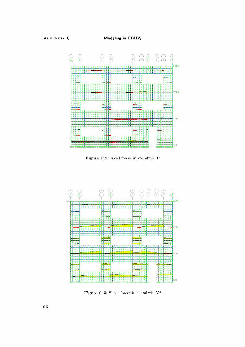
Appendix C Modeling in ETABS
Figure C.2: Axial forces in spandrels, P
Figure C.3: Shear forces in spandrels, V2
96
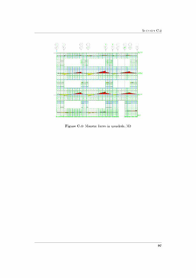
Section C.0
Figure C.4: Moment forces in spandrels, M3
97
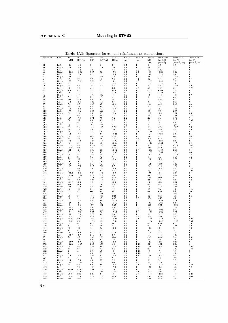
Appendix C Modeling in ETABS
Table C.1: Spandrel forces and reinforcement calculationsSpandrel Loc P P V2 V2 M3 Height Width Force Reinforc. Reinforc. Reinforc.
[kN] [kN/m] [kN] [kN/m] [kNm] [m] [m] M3 for M3 for V for P[kN] [mm2] [mm2/m] [mm2/m]
S1 Left -11 -16 6 8 5 0.7 1 6 15 18 0S1 Right -25 -35 -9 -14 26 0.7 1 38 86 -31 0S2 Left -9 -12 12 7 41 0.7 2.5 59 135 16 0S2 Right -113 -162 107 61 -70 0.7 2.5 -99 -228 141 0S3 Left -49 -70 8 11 -36 0.7 1 -52 -119 25 0S3 Right -10 -14 -37 -52 35 0.7 1 51 116 -120 0S4 Left 28 39 28 16 58 0.7 2.5 83 192 36 91S4 Right -77 -110 123 70 -91 0.7 2.5 -130 -299 161 0S5 Left 2 2 7 10 -52 0.7 1 -75 -172 23 5S5 Right 37 52 -41 -59 21 0.7 1 30 68 -136 120S6 Left 60 85 6 4 38 0.7 2.5 55 126 8 196S6 Right -68 -97 122 70 -76 0.7 2.5 -108 -249 161 0S7 Left -3 -4 27 39 -42 0.7 1 -60 -138 90 0S7 Right 11 16 -15 -22 -4 0.7 1 -6 -14 -50 37S8 Left 3 2 21 18 2 1.2 1 1 3 40 6S8 Right -35 -30 32 26 -8 1.2 1 -7 -16 61 0S9 Left -62 -51 133 111 36 1.2 1 30 70 255 0S9 Right 34 28 107 89 -26 1.2 1 -21 -49 205 64S9 Left 33 28 62 52 12 1.2 1 10 23 119 63S9 Right -63 -52 85 71 -18 1.2 1 -15 -35 163 0S10 Left -77 -64 139 116 41 1.2 1 35 79 267 0S10 Right 19 16 96 80 -20 1.2 1 -17 -39 184 36S10 Left 61 51 75 63 17 1.2 1 14 33 144 117S11 Left -68 -56 104 87 34 1.2 1 29 66 199 0S11 Left 53 44 60 50 14 1.2 1 12 26 115 101S11 Right 6 5 23 19 -3 1.2 1 -2 -5 44 12S12 Left -8 -4 -46 -25 3 1.8 1 1 3 -58 0S12 Right 18 10 -84 -47 174 1.8 1 96 222 -107 23S13 Left 28 16 59 13 266 1.8 2.5 148 339 30 36S13 Right -84 -47 350 78 -259 1.8 2.5 -144 -330 179 0S14 Left -25 -14 44 25 -104 1.8 1 -58 -133 56 0S14 Right 38 21 -75 -42 212 1.8 1 118 270 -96 49S15 Left 40 22 197 44 370 1.8 2.5 205 472 100 51S15 Right -72 -40 488 108 -499 1.8 2.5 -277 -638 249 0S16 Left 16 9 88 49 -267 1.8 1 -149 -342 113 21S16 Right 117 65 -165 -92 101 1.8 1 56 129 -211 149S17 Left 122 68 45 10 212 1.8 2.5 118 271 23 156S17 Right -15 -9 401 89 -362 1.8 2.5 -201 -463 205 0S18 Left 31 17 98 55 -193 1.8 1 -107 -247 125 40S18 Right 14 8 -92 -51 -3 1.8 1 -2 -4 -118 18S19 Left 6 5 61 51 6 1.2 1 5 11 117 11S19 Right 50 42 94 78 -28 1.2 1 -24 -54 179 97S19 Left -8 -6 22 18 3 1.2 1 2 5 41 0S19 Right -66 -55 74 62 -17 1.2 1 -14 -32 142 0S20 Left -92 -76 247 206 57 1.2 1 48 110 473 0S20 Right 62 52 205 171 -48 1.2 1 -40 -92 393 119S20 Left 54 45 110 91 21 1.2 1 17 40 210 104S20 Right -108 -90 160 133 -32 1.2 1 -27 -61 306 0S21 Left -145 -121 312 260 80 1.2 1 67 154 598 0S21 Right 31 26 214 179 -42 1.2 1 -35 -80 411 60S21 Left 68 57 125 104 25 1.2 1 21 47 240 130S21 Right -117 -98 190 158 -36 1.2 1 -30 -69 364 0S22 Left -107 -89 171 143 52 1.2 1 43 99 328 0S22 Right -15 -12 77 64 -7 1.2 1 -6 -14 147 0S22 Left 59 49 71 59 17 1.2 1 14 32 135 113S22 Right 7 6 44 37 -5 1.2 1 -4 -10 84 14S23 Left -2 -1 -43 -24 7 1.8 1 4 9 -55 0S23 Right 16 9 -54 -30 224 1.8 1 124 285 -69 21S24 Left -1 -1 128 28 349 1.8 2.5 194 446 65 0S24 Right -57 -32 420 93 -343 1.8 2.5 -190 -438 214 0S25 Left -16 -9 57 32 -156 1.8 1 -87 -199 73 0S25 Right -44 -24 -97 -54 225 1.8 1 125 287 -123 0S26 Left -132 -73 200 45 396 1.8 2.5 220 506 102 0S26 Right -188 -105 492 109 -476 1.8 2.5 -265 -608 251 0S27 Left -141 -78 137 76 -255 1.8 1 -142 -326 175 0S27 Right -131 -73 177 98 40 1.8 1 22 51 226 0S28 Left -234 -130 449 100 228 1.8 2.5 126 291 229 0S28 Right 175 97 -16 -4 -325 1.8 2.5 -181 -415 -8 224S29 Left 123 68 -113 -63 -238 1.8 1 -132 -304 -144 157S29 Right 15 8 -56 -31 -8 1.8 1 -4 -10 -71 19S30 Left 5 4 77 64 7 1.2 1 6 14 147 10S30 Right 52 44 110 92 -32 1.2 1 -27 -61 210 100S30 Left -8 -7 27 22 3 1.2 1 3 6 51 0S30 Right -72 -60 94 79 -20 1.2 1 -16 -37 181 0S31 Left -107 -89 245 204 60 1.2 1 50 116 469 0S31 Right 28 23 160 133 -34 1.2 1 -28 -65 307 53S31 Left 27 23 80 66 14 1.2 1 12 28 152 52S31 Right -109 -90 169 141 -33 1.2 1 -27 -63 323 0S32 Left -132 -110 229 109 69 1.2 1.75 57 131 251 0S32 Right 54 45 122 58 -28 1.2 1.75 -24 -54 134 103S32 Left 80 67 119 57 24 1.2 1.75 20 47 130 153S32 Right 1 1 36 17 -3 1.2 1.75 -3 -7 40 3S33 Left 2 1 85 21 10 2.3 1.75 4 10 49 2S33 Right -60 -26 157 39 -55 2.3 1.75 -24 -55 90 0S34 Left 1 1 -7 -7 5 1.1 1 4 10 -15 3S34 Right -80 -73 90 82 24 1.1 1 22 51 188 0S35 Left -147 -134 206 75 80 1.1 2.5 73 167 173 0S35 Right 66 60 62 23 -53 1.1 2.5 -48 -110 52 138S36 Left 14 12 -12 -11 -26 1.1 1 -24 -55 -25 29S36 Right -116 -106 184 167 18 1.1 1 16 38 385 0S37 Left -211 -192 372 135 114 1.1 2.5 103 237 311 0S37 Right 256 232 223 81 -110 1.1 2.5 -100 -230 186 534S38 Left 195 177 178 161 -36 1.1 1 -33 -75 371 407S38 Right -45 -41 111 101 -31 1.1 1 -28 -65 232 0
98

Section C.0
Figure C.5: Pier labeling
Figure C.6: Axial forces in Piers, P
99

Appendix C Modeling in ETABS
Figure C.7: Shear forces in piers, V2
Figure C.8: Moment forces in piers, M3
100

Section C.0
Table C.2: Pier forces and reinforcement calculationsPier P P V2 V2 M3 width Height Force Reinf. Reinf.
[kN] [kN/m] [kN] [kN/m] kNm] [m] h[m] from M3 for M3 for V2P1 -517 -45 570 71 74 11.5 0.7 6 15 163P1 -517 -45 570 71 491 11.5 0.7 43 98 163P2 -41 -41 49 41 -8 1 1.2 -8 -18 95P2 -41 -41 49 41 53 1 1.2 53 123 95P3 -132 -132 199 166 -101 1 1.2 -101 -233 381P3 -132 -132 199 166 145 1 1.2 145 334 381P4 -169 -169 195 162 -101 1 1.2 -101 -233 374P4 -169 -169 195 162 140 1 1.2 140 322 374P5 -175 -175 126 105 -70 1 1.2 -70 -160 242P5 -175 -175 126 105 87 1 1.2 87 200 242P6 -517 -45 570 45 1196 11.5 1.1 104 239 104P6 -517 -45 570 45 1784 11.5 1.1 155 357 104P7 -2105 -183 1183 147 2011 11.5 0.7 175 402 338P7 -2105 -183 1183 147 2957 11.5 0.7 257 591 338P8 -144 -144 140 117 -75 1 1.2 -75 -173 269P8 -144 -144 140 117 93 1 1.2 93 214 269P9 -448 -448 386 322 -228 1 1.2 -228 -524 740P9 -448 -448 386 322 236 1 1.2 236 542 740P10 -774 -774 452 377 -253 1 1.2 -253 -581 866P10 -774 -774 452 377 290 1 1.2 290 667 866P11 -739 -739 204 170 -181 1 1.2 -181 -415 391P11 -739 -739 204 170 65 1 1.2 65 149 391P12 -2105 -183 1183 94 4378 11.5 1.1 381 875 215P12 -2105 -183 1183 94 5561 11.5 1.1 484 1112 215P13 -3692 -321 1490 185 5787 11.5 0.7 503 1157 426P13 -3692 -321 1490 185 6880 11.5 0.7 598 1375 426P14 -178 -178 171 142 -55 1 1.2 -55 -127 327P14 -178 -178 171 142 154 1 1.2 154 354 327P15 -829 -829 343 286 -185 1 1.2 -185 -426 658P15 -829 -829 343 286 236 1 1.2 236 542 658P16 -1073 -613 639 304 -474 1.75 1.2 -271 -622 699P16 -1073 -613 639 304 309 1.75 1.2 176 406 699P17 -2080 -238 1153 120 3453 8.75 1.1 395 907 275P17 -2080 -238 1153 120 4654 8.75 1.1 532 1223 275P18 -1612 -921 338 175 -160 1.75 1.1 -91 -210 403P18 -1612 -921 338 175 606 1.75 1.1 346 796 403
101


References
[1] ANSYS, version 10.0, User and Theoretical Manual, ANSYS, Inc., Southpointe,Canonsburg, Pennsylvania, USA
[2] ATC, The Seismic Evaluation and Retro�t of Concrete Buildings, Applied Technol-ogy Council, ATC-40 Report, Redwood City, California, USA, 1996
[3] Bessason, Bjarni & Sigfússon, Thordur Capacity and earthquake response analysis ofRC-shear walls, Nordic concrete research, vol. 27:1-14, Oslo, Norway, 2001
[4] Chen, W.F, Plasticity in Reinforced Concrete, John Wiley & Sons, Inc., New York,USA, 1982
[5] Chopra, Anil K., Dynamics of Structures: Theory and Applications to EarthquakeEngineering, Prentice Hall, New Jersey, USA, 2001
[6] Cook, Robert D., Concepts and Applications of Finite Element Analysis, John Wiley& Sons, Inc., New York, USA, 2002
[7] DS411, Norm for betonkonstruktioner, eng. Code of Practice for the Structural useof Concrete (in Danish), Dansk Standard, Copenhagen, Denmark, 1999
[8] ETABS, Concrete Shear Wall Design Manual, Version 8, CSI, Computer & Struc-tures, Inc., Berkeley, USA, 2002
[9] Eurocode 2, Design of Concrete Structures. EN1992-1-1, European Commitee forStandardization, Brussels, 2004
[10] Eurocode 8, Design of Structures for Earthquake Resistance. EN1998-1-1, EuropeanCommitee for Standardization, Brussels, 2003
[11] Fajfar, P., A nonlinear analysis method for performance-based seismic design, Earth-quake Spectra, 16, p. 573-593, 2000
[12] Gulvanessian, Haig, Designers' Guide to EN 1998-1 and EN 1998-5, Thomas Telford,London, UK, 2005
[13] Jensen, Bjarne Chr., Betonkonstruktioener efter DS411, 2. udgave (in Danish), In-geniørenbøger, Copenhagen, Denmark, 2003
[14] Jónsson, Kristján, MATLAB, forritunarmál fyrir vísindalega útreikninga (in ice-landic), Útgáfufélagið Slemba, Reykjavík, Iceland, 2004
[15] Moaveni, Saeed, Finite Element Analysis, Theory and Applications with ANSYS,Person Educations, Inc., New Jersey, USA, 2003
103

References
[16] Nanakorn, P. and Soparat, P., Finite Element Analysis of Cracking Localization:The Smeared Crack Approach with a Mixed Formulation, Thammasat InternationalJournal of Science and Technology, Vol. 5, No. 3, pp. 28-39, 2000.
[17] Nawy, Edward G and Scanlon, Andrew Designing Concrete Structures for Service-abilty and safety, American Concrete Institute, Detroit, USA, 1992
[18] Nielsen, M.P., Limit Analysis and Concrete Plasticity, Second Edition, CRC Press,USA, 1999
[19] Nilson, Arthur H, Finite Element Analysis of Reinforced Concrete, American Societyof Civil Engineers, New York, USA, 1982
[20] O'Brien, Eugene J & Dixon, Andrew S, Reinforced and Prestressed Concrete Design,The Complete Process, Longman, Edinburgh, UK, 1999
[21] Pauley, Priestley, Seismic Design of Reinforced Concrete and Masonry Buildings,John Wiley & Sons, Inc., New York, USA, 1992
[22] SAP2000, Analsysis Reference Manual, Version 8, CSI, Computer & Structures, Inc.,Berkeley, USA, 2002
[23] Sigbjörnsson, Ragnar SOUTH ICELAND EARTH-QUAKES 2000: Damage and Strong-Motion Recordings,http://www.eaee.boun.edu.tr/bulletins/v20/v20web/iceland.htm,
[24] Stefansson, Ragnar, Gudmundsson, Gunnar B. & Halldorsson, Pall, The South Ice-land earthquakes 2000 a challenge for earthquake prediction research, Reykjavík,2003, http://www.vedur.is/utgafa/greinargerdir/2003/03017.pdf
[25] Teknisk Ståbi, 18. udgave (in Danish), Ingeniørenbøger, Copenhagen, Denmark, 2002
[26] Wilson, Edward L, Three Dimensional Static and Dynamic Analysis of Structures,A physical Approach with Empahsis on Earthquake Engineering, CSI, Computer &Structures, Inc., Berkeley, USA, 2002
104