analysis on the effects of housing policy for rural areas

Analysis on the Effects of Housing Policy for Rural Areas in Korea: Using System Dynamics Model

Copyright 2013 Korea Research Institute for Human Settlements

All rights reserved. Printed in the Republic of Korea. No part of this publication may be reproduced in any manner without written permission from KRIHS except in the case of brief quotations embodied in critical articles and reviews. For more information, please address inquiries to: Korea Research Institute for Human Settlements, 1591-6, 254 Simin-daero, Dongan-gu, Anyang-si, Gyeonggi-do, 431-712, Korea.

Tel: +82.31.380.0594Fax: +82.31.380.0470Website: http://www.krihs.re.kr

Note: The Special Report Vol. 24 is a summary of a chapter in the report titled “A Rural Housing Policy for Improving Housing Service Level” published by the KRIHS in 2012.

Analysis on the Effects of Housing Policy for Rural Areas in Korea: Using System Dynamics Modelby Kang Mi-na-- Anyang : Korea Research Institute for Human Settlements, 2013 p. ; cm. -- (KRIHS special report ; 2013-24)

ISBN 978-89-8182-221-7 94300 : Not for saleISBN 978-89-8182-991-9(set) 94300

335.8-KDC5363.5-DDC21 CIP2013027227

Chapter 1. Introduction _ 1

Chapter 2. Identification of Housing Service Index _ 7

1. Hedonic Price Model of Housing ………………………………………………………… 92. Housing Price Model and Rental Price Model …………………………………………… 103. Identification of Housing Service Index ………………………………………………… 17

Chapter 3. Development of System Dynamics (SD) Model to Analyze the Effects of Housing Policy for Rural Area _ 21

1. System Dynamics Model ………………………………………………………………… 222. Consideration on Housing Policy for Rural Area ………………………………………… 243. Criteria of the Model ……………………………………………………………………… 274. Composition of Model …………………………………………………………………… 29

Chapter 4. Analysis on Policy Effects _ 45

1. Policy to Increase Supply for Rental Housing …………………………………………… 472. Support for Housing Purchase and Cost on Rental House ……………………………… 493. Effects of Low-Interest Rate Loan (Support for Expenses on Refurbishment and Repair)

…………………………………………………………………………………………… 514. Effects of Housing Allowance / Housing Voucher System ……………………………… 525. Housing Market Stabilization Policy: Application of Housing Price Ceiling System …… 546. Overall Comparative Analysis on Policy Effects ………………………………………… 55

Chapter 5. Conclusion _ 57

Reference _ 60

_______________

_______________

_______________

_______________

Contents

_______________

_______________

_______________

_______________

_______________

_______________

Table 1 Rural Area Housing Conditions Indicator (as of 2010) ……………………………… 4

Table 2 Mean Value and Median Value of Variables in Housing Price Function …………… 13

Table 3 Mean Value and Median Value of Variables in Rental Housing Price Function ……… 13

Table 4 Estimation Results of Housing Price Model ……………………………………… 15

Table 5 Estimation Results of Rental Price Model ………………………………………… 16

Table 6 Housing Service Index …………………………………………………………… 19

Table 7 Current Policies Related to Housing in Rural Area ……………………………… 25

Table 8 Classification of Housing Policy for Rural Area ………………………………… 26

Table 9 Definition of Input and Output in Sub-models in Integrated Model of

Population, Households and Housing …………………………………………… 30

Table 10 Definition of Input and Output in Sub-models of Regional and Household Income

…………………………………………………………………………………… 36

Table 11 Indicator to Measure the Effects of Housing Policy for Rural Area ……………… 40

Table 12 Definition of Input and Output in Housing Policy for Rural Area Model ………… 41

Table 13 Effects of Rental Housing Supply Expansion Policy (based on 2020) …………… 48

Table 14 Changes in Quantitative Indicator of Housing upon Expansion of Housing

Supply in Rural Area …………………………………………………………… 48

Table 15 Policy Effects of Supporting Low-Interest Rate for Housing Purchase Loan

(based on 2020) ………………………………………………………………… 50

Table 16 Social Cost Estimate upon Support for Low-Interest Rate for Housing Purchase

Loan……………………………………………………………………………… 50

Table 17 Policy Effect of Supporting Low-Interest Rate Loan for Housing Refurbishment

and Repair (based on 2020) ……………………………………………………… 52

Table 18 Effect of Housing Allowance/Housing Voucher Policy ………………………… 53

Table 19 Effect of Expanding the Discount of Housing Price Ceiling System

(based on 2020) ………………………………………………………………… 54

Table 20 Comparative Analysis on Housing Service Level Improvement Compared to

Social Cost for Each Policy ……………………………………………………… 56

Table

Figure 1 Procedure for the Establishment of System Dynamics Model ……………………23

Figure 2 Conceptual Map of Model Development for Rural Housing Policy Effect ………… 27

Figure 3 System Flow of National Population …………………………………………… 31

Figure 4 System Flow of Population in Cities and Province……………………………… 32

Figure 5 System Flow of Households……………………………………………………… 33

Figure 6 System Flow of Housing ………………………………………………………… 34

Figure 7 System Flow of GDP …………………………………………………………… 37

Figure 8 System Flow of GRDP…………………………………………………………… 38

Figure 9 System Flow of Household Income ……………………………………………… 39

Figure 10 System Flow of Housing Policy ………………………………………………… 42

Figure 11 Prospects for Future Housing Conditions in Rural Area and the Model Framework

of the Policy Effect Analysis …………………………………………………… 44

Figure

Kang Mi-na She is a Research Fellow of the Housing & Land Research Division at the Korea Research Institute for Human Settlements. She received her Ph.D. in Economics at the Pennsylvania State University, USA. Her major research fields are housing welfare and policy in the housing and the real estates. Recent research works

include 「A Rural Housing Policy for Improving Housing Service Level」 (2012), 「A Study on Housing Policy for Disabled Household」 (2010), 「Analysis of the Single Family Detached Housing Market to Promote the Diversity of Housing Types」 (2009), 「A Study on Social Integration of the Nest- Housing District」 (2009), 「A Study on Housing Support System for the Elderly Based on Housing Demand Analysis」 (2008), 「2006, 2007, 2008, 2010 Korea Housing Survey」 (2007, 2008, 2009, 2011), 「A Study on Demand Estimation of National Rental Housing」 (2007), 「A Study on Housing Service Disparity among Regions and Classes (II): Policy Measures for Improving Housing Welfare」 (2006), etc.

Author

Summary

In Korea, rural areas have been serving as an important basis for living for a long time. However, the status of rural areas has been weakened with a rapid decrease in population and households in rural areas and inflow of population into cities due to urbanization and industrialization. Many problems have occurred in rural areas including worn-out homes or vacant houses. In the meantime, new trend of returning to farming and rural areas has emerged as many people want to live in nature after retirement or people want to live a brand new life in rural areas. Now is the time to review the living conditions and environment in rural areas to make the areas more livable place for many people.

In quantitative terms, the housing conditions in rural areas are good with the appropriate number of houses but the ratio of vacant home is high, which serves as a major factor in deteriorating living environment. In qualitative terms, the issues of safety and convenience emerge as there are many old and rundown houses. In addition, the possibility of refurbishing or repairing the houses is low as most residents in the old house are the elderly.

This study defines rural areas as administrative districts classified into town and township and rural housing as the house located in rural areas. The purpose of this study is to analyze the effects of housing policy on rural areas and identify the most effective policy. To this end, “housing service indicator”, which shows qualitative conditions of housing, was developed along with quantitative indicator on housing and living conditions. In addition, a simulation model was developed using system dynamics (SD) by identifying the causal relationship among various elements that compose the rural society. Based on the model, this study expects future housing conditions in rural areas, measures effects of the housing policy and compares policy programs designed to improve living conditions in rural areas.

The development of SD model to analyze the effects of housing policy for rural areas is a huge task. 7 processes are required to develop the model: designing various sub-models that compose the society, identifying causal relationship among variables in individual sub-model and system flow, establishing a model, analyzing the behavior of model, evaluating the feasibility, analyzing policy and making a decision. Population Housing Integration Model, Regional Income and Household

Summary

Income Model and Housing Policy Model were established as a big model and 17 sub-models were established under them. Based on the model, a future housing market in rural areas was expected and policy effects including quantitative effects like housing supply rate and the number of housing units per 1000 persons and qualitative effects like living conditions and required financial resources to implement the policy were estimated.

Policy effects against costs were weighed and analyzed using SD model and the result shows that the policies that could lead to the most significant improvement in housing conditions for rental house in rural areas are the ones that support housing purchase and fund for rent followed by housing allowance and housing voucher system, which are living cost subsidy system designed for households that belong to the second income quantile or lower.

This study is meaningful in that it developed “housing service indicator”, which shows the quality of living conditions, expects future housing and living conditions in rural areas, and calculates the effects of housing policy and social costs required to implement the policy. Existing studies have limitations regarding the model establishment and analysis on rural housing conditions. In this regard, this study opens a new chapter for rural housing policy research.

KRIHSSPECIAL REPORT2013

Introduction

2

Introduction

Rural areas have long been the basis for people’s lives in Korea. Rice paddy has been the important basis as rice is the staple food for Koreans. However, the status of rural areas has been weakened with a rapid decrease in population and households in rural areas and inflow of population into cities due to urbanization and industrialization. Many problems have occurred in rural areas including worn-out homes, vacant houses and the increasing number of closed schools. It is considered that the development of agricultural technology and automation play a significant role in reducing agricultural population though the share of agricultural land in national territory shows no big changes from 22% in 1949 to 20% in 2010.

In the meantime, a new trend of returning to farming and rural areas has emerged as many people want to live in nature after retirement or people want to live a brand new life in rural areas. Unfortunately, it is true that much less attention has been paid to living conditions and housing policy for rural areas than those for urban areas. Now is the time to review the living conditions and environment in rural areas to make them more livable place for many people.

This study defines rural areas as administrative districts classified into town and township and rural housing as the house located in rural areas. The purpose of this study is to analyze the effects of housing policy on rural areas and identify the effectiveness of the policy. To this end, an indicator to evaluate the housing service levels of rural areas is developed and a model to analyze policy effects is established so that the most effective policy can be identified after comparing and analyzing social costs and living conditions in rural areas from both qualitative and quantitative terms.

3


The scope of this study is classified into rural areas (town and township) and urban areas (village) and the model was established for each city and province from spatial perspective. From time perspective, the scope covers from the year of 2000 to the year of 2040 to establish the model based on existing data.

The effect of housing policy influences the number of housing stock and old and defective houses in a certain beneficial area as a whole. But at the same time, the policy directly impacts each individual household located in the area, leading to improvement of housing conditions of an individual household. It is not easy, however, to identify the improvement of housing conditions for each household as there is no objective data developed. Therefore, quantitative indicators including population size, the number of households and houses and housing supply rate have been used to design and evaluate the housing policy due to the convenience of data production and absence of appropriate indicators. It is important to develop an indicator that shows not only quantitative changes but also housing condition changes of individual household to identify the effects of housing policy for rural areas. In general, housing supply rate, the number of houses per 1000 persons, and the ratio of empty houses have been used as quantitative indicators. The number or share of households that do not meet the minimum housing standard and the levels of housing deterioration have been used as proxy variables for qualitative indicators to evaluate the housing conditions of rural areas. As indicators that show market condition, price income ratio (PIR) which indicates the relationship between market price of housing and annual household income and rent income ratio (RIR) which shows the level of rent have been used. These variables show the conditions of the overall region so they are not sufficient enough to be used as indicators that evaluate housing conditions of individual household.

Looking at the current housing conditions of rural areas in Korea based on existing indicators, the number of housing units per 1000 persons is 389.2 as of 2010 and the housing supply rate (based on the existing housing supply rate) is 103% in quantitative terms. It seems that there is no significant problem related to housing stock. One of the problems that lowers the quality of housing conditions in rural areas is empty houses. It is shown that the share of empty house in housing stock in rural areas is 9.9%.

From the qualitative perspectives, the number of households that do not meet the minimum housing standard is 478,000 or 14.5% of total households in rural areas as of 2010. 88.2% of the households are classified into below-standard households due to

4

their facilities. About 34% of rural households live in more than 20-year-old houses, which led to severe levels of the rural housing deterioration. The share of the elderly living in more than 30-year-old housing is even higher, reaching about 44%. In many cases, the elderly households have low fixed income so they cannot have capacity to refurbish or repair their houses even though safety issues associated with housing arise.

PIR, which is a market indicator, is 2.7 times and RIR is 18.2% based on median value. The PIR figure can be interpreted that a house can be purchased if one collects rural household income for 2.7 years and RIR figure means that 18.2% of rural household monthly income were used for rent. Given the PIR for urban areas, which is 5 times higher than that of rural areas, the share of rental cost in rural areas is relatively small. However, the data should be interpreted given the fact that there are not many housing transactions as many people live in the same place for a long time in rural areas. Assuming that critical point of RIR is 30% of monthly income, the burden of rent in rural areas is not too high compared to that of urban areas.

Table 1 Rural Area Housing Conditions Indicator (as of 2010)

Classification Major Indicators Calculation Formula Indicator Value

Quantitative Indicator

Housing Supply Rate (%)Existing Housing Supply Rate= (Rural Housing Stock/The Number of Households in Rural Area) X 100

103%

The Number of Housing Units per 1000 Persons

(No.)Rural Housing Stock/Rural Population 389.3

Ratio of Empty House (%)(The Number of Empty Houses in Rural Area/Rural Housing Stock) X 100

9.9%

Qualitative Indicator

Housing Service Conditions

The Number of Households that Do Not Meet Minimum Housing Standard (Area, Facility, Bedroom)

478,000 Households (14.5% of Rural

Households)

Level of Housing Deterioration (The Share of Houses More than 30-Years-Old)

34.1%

Market Indicator

PIRHousing Market Price/Annual Household Income

2.7 Times based on Median Value

RIR Rent/ Monthly Household Income18.2% based on Median Value

Source: Ministry of Land, Infrastructure and Transport, Korea Research Institute for Human Settlements. 2010

Korea Housing Survey

5


This study evaluates the housing service levels of individual household using quantitative indicators as well as system dynamics method and develops integrated indicators by the region and household characteristics, making it possible to conduct comparative analysis on the effects of housing policy.

To this end, 6 sub-models (population, household, housing, living, household income and policy) are established. “Prospects on Rural Housing and Policy Effect Measurement System” was developed to forecast the future rural housing environment and apply specific items required for the implementation of rural housing policy. This model can support a reasonable decision-making process from the long-term perspective as it considers various elements in rural housing environment to measure policy effects in a quantitative and comprehensive way. The development of housing policy based on comparative analysis on policy effects justifies the implementation of policy and gives confidence on the developed policy to decision-makers, leading to continuity of the policy.


Identification of Housing Service Index

8

There are quantitative, qualitative and market indicators that show housing conditions. In this chapter, housing service indicator that shows housing conditions of individual household in rural areas is developed to analyze policy effects.

It is not easy to measure levels of housing service provided by various types of houses with one criteria as housing is composed of a number of elements. However, the criteria and method with which objective measurement of housing service is possible are required to identify reasonable housing policy. Therefore, in this chapter housing service levels are measured objectively and ‘willingness to pay’ function related to housing service by households that consume housing service is identified using the Hedonic Price method.

The order of developing housing service index that shows relative housing conditions by region and occupancy type is as follows. First, housing service model that calculates housing service level depending on the housing quality should be established through two steps. In the first step, the relationship between housing price and housing quality is standardized using the 2010 Korea Housing Survey. In the second step, housing quality is converted into housing service index. In the final stage, housing service levels shown by different household income levels are identified by conducting regression analysis on household income, attribute, and housing service levels.

Identification of Housing Service Index

9


1. Hedonic Price Model of Housing

Unlike other goods, housing is an assembly composed of different elements including rooms, living room, and dining room. Depending on the size and the number of the elements, the market price of housing changes. Housing prices can be different not only based on structural attributes but also based on environmental attributes including location and region where housing is located. Therefore, buying a housing means buying a bundle of attributes that compose housing. Assuming that “the value of a housing is dependent on attributes that compose the housing”, the housing price is determined by price and quantity of attributes included in the housing. Here, the marginal price of attribute is called ‘hedonic’ or ‘implicit’ price.

The relationship between attributes and housing price can be presented in the following function.

P = f(S, A, L, N) (Formula 1)Here, P : Price of a house S : A bundle of housing structural attributes A : Area of land L : Locational attributes N : Neighborhood attributes

In case of analyzing housing market, Hedonic Price model selects an appropriate formula out of linear, semi-log or double-log formulas. This research selects the double-log formula in Hedonic Price model as below.

P = KAαS1β1…S1

β1L1γ1…Lm N1 …Nn exp(ε1D1+…+ε zD z) (Formula 2)

Here, α, β1,…, β1, γ1,…, γm , δ1, …, δn , ε1, …, ε z : various parameters K : Constant value D : Dummy variable

γm δ1 δn

10

In Hedonic Price model, the hedonic price of a certain attribute is presented in the gradient of the attribute. In other words, the gradient can be interpreted as the willingness to pay by households for marginal changes of the attribute. For example, hedonic price of S1 and PS1 which is the willingness to pay for S1 can be presented as below.

PS1 = β1 (Formula 3)

As shown in this formula (formula 3), the hedonic price of S1 is determined by housing price elasticity (β1), price of house (P) and the size of S1.Meanwhile, the willingness to pay for housing structure S1 can be determined by household attributes including household income, age of home owner, number of people in a household and occupation as well as the size of S1 from the perspective of household which consumes housing service. Therefore, the function of willingness to pay related to housing structure S1 can be presented as below (formula 4).

PS1 = g(S1, Y, Z) (Formula 4)Here, S1 : A bundle of housing attributes for 1st household Y : Household income Z : A bundle of attributes

2. Housing Price Model and Rental Price Model

Housing service level model is intended to calculate the levels of housing services depending on housing quality. By using the data from 2010 Korea Housing Survey, the relationship between housing price and housing quality is standardized, housing quality is converted into housing service index and regression analysis is conducted on household income, attributes and housing service levels. Finally, the housing service levels consumed by different levels of household income are identified. Formula 2 is converted as follows to identify Hedonic Price model through regression analysis.

pS1

11


Price of a house = f(Building year, housing usage area, the number of rooms, housing type, kitchen type, flush toilet, supply of hot water, water works, whether the location belongs to city or province and whether the location belongs to city or county)

P = KS1 S2 S3 exp(β1S4 + β2S5 + β3S6 + β4S7) (Formula 5) exp(γ1S8 + γ2S9 + γ3S10 + γ4S11) exp(δ1L1 + … + δ15L15)exp(εD)

Here P : Housing or rental housing price S1…S3 : Variables including building year, housing usage area, number of

bedrooms S4…S7 : Dummy variables that show housing type including single family

house, apartment, row house, multiplex house, other types of house S8…S11 : Dummy variables that show housing facilities including kitchen type,

flush toilet, supply of hot water, water works L1…L15 : Dummy variables that show whether the location belongs to city or

province like Seoul City … Southern Gyeongsang Province D : City=1, County=0

Table 2 and Table 3 show the mean value, median value and ratio of dummy variables regarding the variables used in the hedonic price function based on the housing survey data. The housing price used in housing price function as a dependent variable in Table 2 shows that the average housing price is 210 million won and its median value is 140 million won. The life span of housing is 17.8 years on average with median value of 13 years. The usage area of housing is 84㎡ as median value and this seems to be attributed to the supply of houses based on apartment supply standard. The average number of rooms is 2.9, which is almost three. In terms of housing type, the share of single family house is 35%, apartment is 54%, row house is 5%, multiplex house is about 5%. Regarding internal facilities, 96% of houses are equipped with stand-up type kitchen, flush toilet, hot water supply and water works. In particular, 99% of owner-occupied homes are equipped with flush toilet.

α1 α2 α3

12

Table 3 presents the variables of rental housing price function. Rental housing system which is called ‘Jeon-se’ is Korea’s unique type of housing rent. This type of rent is based on a big deposit. The other type is monthly rent with or without security deposit. Simply put, under the rent with a big deposit system, a lessee pays a substantial sum of money at once upon rental contract to a lessor. When the rental contract expires, the lessor gives the money back to the lessee again. It can be said that a lessor is given the interest of the money as rent by the lessee upon rental contract.

Lessees prefer rent with a big deposit type because they can receive the money back when a rental contract expires even though a significant sum of money should be paid at once. Under the monthly rent with security deposit type, a lessee should pay monthly rent after depositing some money to the lessor. The monthly rent without security deposit system is similar to that of other countries under which a lessee pays agreed monthly fee to a lessor. In the rental housing price model, the monthly rent with or without security deposit are converted into the rent with a big deposit price to encompass all types of rental housing. The monthly rent conversion rate uses 10%, which is commonly used in Korea Appraisal Board, Kookmin Bank or real estate agencies.

The housing rental price used as a dependent variable is 60 million won on average with median value of 40 million won. The life span of rental housing is 16 years on average with median value of 13 years. The usage area of house is 50㎡ as median value, which is 34㎡ smaller than that of owner-occupied home. It seems that most rental houses are used by households in the family formation period including single household, newly-married couple household or household with young children and they prefer a smaller size and cheaper house than home owners. The share of single family house is about 47%, apartment is about 41%, row house is 4%, and multiplex house is about 6%. Compared to owner-occupied houses, the share of single family house and multiplex house is higher and apartment is lower. Regarding internal facilities, more than 95% rental houses are equipped with stand-up type kitchen, flush toilet, hot water supply and water works. Compared to owner-occupied homes, however, the ratio of having stand-up type kitchen, flush toilet and hot water supply facility is lower.

13


Table 2 Mean Value and Median Value of Variables in Housing Price Function

Variable Name Unit Mean Value or Ratio Median Value

Housing Price10,000 won

21,016 14,000

Life Span of Housing Years 17.8 13

Usage Area m2 98.1 84

Number of Rooms No. 2.9 3

Single Family House (YES=1) - 0.3475 -

Apartment (YES=1) - 0.5431 -

Row House (YES=1) - 0.0473 -

Multiplex House (YES=1) - 0.0536 -

Stand-up Kitchen (YES=1) - 0.9903 -

Flush Toilet (YES=1) - 0.9602 -

Bathroom with Hot Water Supply (YES=1) - 0.9719 -

Installation of Waterworks (YES=1) - 0.9653 -

Table 3 Mean Value and Median Value of Variables in Rental Housing Price Function

Variable Name Unit Mean Value or Ratio Median Value

Rental Housing Price 10,000 won 6,210 4,100

Life Span of Housing Years 16.4 13

Usage Area m2 54.4 50

Number of Rooms No. 2.2 2

Single Family House (YES=1) - 0.4680 -

Apartment (YES=1) - 0.4121 -

Row House (YES=1) - 0.0429 -

Multiplex House (YES=1) - 0.0594 -

Stand-up Kitchen (YES=1) - 0.9834 -

Flush Toilet (YES=1) - 0.9752 -

Bathroom with Hot Water Supply (YES=1) - 0.9565 -

Installation of Waterworks (YES=1) - 0.9936 -

Table 4 and Table 5 show parameters identified after regression analysis on Korea housing survey data based on formula 5. Independent variables in the two tables are the same. However, Table 4 uses housing price and Table 5 uses rental housing price as a

14

dependent variable. Monthly rental fee is converted into rent with a big deposit price by applying the annual interest rate of 10%. In Table 4, adjusted R2 value is 0.727 and t which shows statistical significance of all parameters is statistically significant.

The estimation of variables which show physical characteristics of housing in the housing price calculation model demonstrates that the longer the house has been in use, the lower price it has and housing price increases with the increase of house size and the number of rooms. In terms of housing type, the price of multiplex, row, and single family houses is relatively lower than that of apartment. Installation of stand-up kitchen, flush toilet, bathroom with hot water supply and water works serve as a factor that increases the housing price. All the results are in line with theory and common sense beliefs. Meanwhile, review on dummy variables that show regional characteristics finds that the housing in Seoul, Gyeonggi-do and Incheon has the most significant influence on housing price. Houses located in cities have a stronger positive relationship with housing price. The most influential variable for the price of owner-occupied home is the dummy variable of housing location in Seoul. Housing located in Jeonbuk and Jeonnam provinces serves as the factor in lowering housing price. This is because these provinces includes rural areas where noticeable decline in population and households is witnessed.

Table 5 summarizes the estimation based on rental housing price model. In the table, a dependent variable is rental housing price and R2 which was adjusted to have statistical significance is 0.477 and t which shows statistical significance of all parameters is statistically significant.

The estimation of variables which present physical characteristics of housing in the housing price calculation model shows that the longer the house has been in use, the lower rental price it has and housing rental price increases with the increase of house size and the number of rooms. In terms of housing type, the rental price of multiplex, row, and single family houses is relatively lower than that of apartment. Installation of stand-up kitchen, flush toilet, bathroom with hot water supply and water works serve as a factor that increases rental housing price. However, the size is half of owner-occupied homes’ size. The most influential variable for the price of rental housing is the dummy variable of housing location in Seoul. Rental price of housing located in provinces that encompass relatively large rural areas (Jeonbuk and Jeonnam, Gangwon, Gyeongbuk and Gyeongnam) is less influenced by location than price of owner-occupied housing. This is because moving is less frequent in rural areas.

15


Table 4 Estimation Results of Housing Price Model

Adjusted R2 Variable Name Parameter Coefficient t-StatisticsSignificance

Level

0.727

Constant Value K 5.532 1452.289 0.000

Life Span of Housing α1 -0.221 -870.859 0.000

Usage Area α2 0.722 1467.550 0.000

Number of Rooms α3 0.409 484.683 0.000

Single Family House (Y/N) β1 -1.033 -524.814 0.000

Apartment (Y/N) β2 -0.642 -328.584 0.000

Row House (Y/N) β3 -1.113 -529.681 0.000

Multiplex House (Y/N) β4 -1.178 -563.818 0.000

Stand-up Type Kitchen (Y/N) γ1 0.227 101.635 0.000

Flush Toilet (Y/N) γ2 0.359 288.254 0.000

Bathroom wi th Hot Water Supply (Y/N)

γ3 0.242 165.058 0.000

Installation of Waterworks (Y/N) γ4 0.346 323.602 0.000

Seoul (Y/N) δ1 1.145 660.536 0.000

Busan (Y/N) δ2 0.086 48.127 0.000

Daegu (Y/N) δ3 0.016 8.666 0.000

Incheon (Y/N) δ4 0.455 247.708 0.000

Gwangju (Y/N) δ5 -0.271 -139.878 0.000

Daejeon (Y/N) δ6 0.127 64.286 0.000

Ulsan (Y/N) δ7 0.181 89.887 0.000

Gyeonggi (Y/N) δ8 0.575 334.075 0.000

Gangwon (Y/N) δ9 -0.274 -142.700 0.000

Chungbuk (Y/N) δ10 -0.163 -85.533 0.000

Chungnam (Y/N) δ11 -0.198 -106.487 0.000

Jeonbuk (Y/N) δ12 -0.483 -260.241 0.000

Jeonnam (Y/N) δ13 -0.455 -245.338 0.000

Gyeongbuk (Y/N) δ14 -0.291 -161.884 0.000

Gyeongnam (Y/N) δ15 -0.103 -57.854 0.000

City (Y/N) ε 0.413 666.969 0.000

16

Table 5 Estimation Results of Rental Price Model

Adjusted R2 Variable Name Parameter Coefficient t- StatisticsSignificance

Level

0.477

Constant Value K 4.881 889.211 0.000

Life Span of Housing α1 -0.195 -626.017 0.000

Usage Area α2 0.677 975.392 0.000

Number of Rooms α3 0.055 60.950 0.000

Single Family House (Y/N) β1 -0.189 -95.979 0.000

Apartment (Y/N) β2 -0.022 -10.793 0.000

Row House (Y/N) β3 -0.300 -133.302 0.000

Multiplex House (Y/N) β4 -0.126 -57.983 0.000

Stand-up Type Kitchen (Y/N) γ1 0.013 5.783 0.000

Flush Toilet (Y/N) γ2 0.317 153.221 0.000

Bathroom with Hot Water Supply (Y/N)

γ3 -0.059 -37.118 0.000

Installation of Waterworks (Y/N)

γ4 0.596 181.067 0.000

Seoul (Y/N) δ1 0.845 323.424 0.000

Busan (Y/N) δ2 0.160 58.782 0.000

Daegu (Y/N) δ3 0.137 49.767 0.000

Incheon (Y/N) δ4 0.241 87.407 0.000

Gwangju (Y/N) δ5 -0.202 -68.404 0.000

Daejeon (Y/N) δ6 0.187 64.443 0.000

Ulsan (Y/N) δ7 0.354 116.319 0.000

Gyeonggi (Y/N) δ8 0.496 189.746 0.000

Gangwon (Y/N) δ9 -0.084 -28.793 0.000

Chungbuk (Y/N) δ10 0.072 24.404 0.000

Jeonnam (Y/N) δ11 0.093 32.780 0.000

Jeonbuk (Y/N) δ12 -0.059 -20.242 0.000

Jeonnam (Y/N) δ13 -0.082 -27.607 0.000

Gyeongbuk (Y/N) δ14 0.089 31.366 0.000

Gyeongnam (Y/N) δ15 0.089 32.171 0.000

City (Y/N) ε 0.236 197.969 0.000

Note: Rent with or without security deposit is converted into rent with a big deposit, Jeon-se. Full Deposit of

Rental Housing = (Security Deposit) + (Monthly Rent X 12 / 0.1)

17


3. Identification of Housing Service Index

In the previous part, characteristics of variables used in housing price and rental housing price analysis model on Korea housing survey data are summarized and compared. Also, the estimation of housing price model and rental housing price model is made and analyzed. In this part, the basis housing should be established to get housing service levels. It is desirable to select housing with average or higher quality as the basis. Statistics on variables related to housing facilities to establish the basis housing include mean and median values of member variables and ratio to dummy variables in Table 2 and Table 3, which are based on housing survey data. These values are used to identify the housing service levels of basis housing, which shows the national average housing quality.

Housing that can serve as the basis is selected virtually to identify standardized housing service index, which can be applied widely to individual housing nationwide. To reflect the conditions of housing market correctly, the basis housing is classified into owner-occupied housing and rental housing. Given the mean and median values drawn from the statistical analysis, the basis housing for owner-occupied housing is established as an apartment located in Daegu Metropolitan City, which has been in use for 14 years with 85㎡ usage area, three bedrooms, stand-up type kitchen, flush toilet, bathroom with hot water supply and waterworks. Meanwhile, considering the mean and median values, the basis housing for rental housing is established as an apartment located in Daegu Metropolitan City, which has been in use for 13 years with 50㎡ usage area, two bedrooms, stand-up type kitchen, flush toilet, bathroom with hot water supply and waterworks.

If facilities and attributes of owner-occupied basis housing are put into formula 5, a certain value that reflects the physical facility conditions of the basis housing is calculated at 36.807. This value is converted into 100.0 as owner-occupied household housing service index and housing service index of all owner-occupied houses (S1i) is calculated based on facility conditions.

18

S1i = [{Bui lding Year -0 .221· Usage Area 0.722·Number of Rooms 0.409·EXP(-1.033×Single Family House-0.642× Apartment-1.113×Row House-1.178×Multiplex House)·EXP(0.227×Stand-up Type Kitchen+0.359×Flush Toilet+0.242× Bathroom with Hot Water Supply+0.346× Installation of Waterworks)}/36.807]×100

Similar to owner-occupied housing, if facilities and attributes of basis rental housing are input into formula 5, a certain value that reflects the physical facility conditions of the basis rental housing is calculated at 20.726.

This value is converted into 100.0 as tenant household housing service index and housing service index of all rental housing (S2i) is calculated based on facility conditions.

To compare owner-occupied housing, rental housing, rural areas and overall nation, housing service index for the whole owner-occupied housing is put as 100 and relative housing service index for tenant household (S*2i) is calculated.

S2i = [{Building Year-0.195·Usage Area0.677·Number of Rooms0.055·EXP(-0.189×Single Family House-0.022×Apartment-0.300×Row House-0.126×Multiplex House)·EXP(0.013×Stand-up Type Kitchen+0.317×Flush Toilet-0.059×Bathroom with Hot Water Supply+0.596×Installation of Waterworks)}/20.726]×100

S*2i = [{Bui lding Year -0 .221·Usage Area 0.722·Number of Rooms 0.409·EXP(-1.033×Single Family House-0.642×Apartment-1.113×Row House-1.178×Multiplex House)·EXP(0.227×Stand-up Type Kitchen+0.359×Flush Toilet+0.242×Bathroom with Hot Water Supply+0.346×Installation of Waterworks)/36.807]×100

Through the process explained above, housing service index (2005 national owner-occupied household =100) is presented in Table 6. Overall, rural housing service level is lower than the national housing service level and in particular, the housing service level of tenant household in rural areas shows the worst condition. As of 2013, housing service level of rural tenant household is 98.8, and that of rural owner-occupied household is 100.3 respectively, which are lower than the national housing service level.

19


Table 6 Housing Service Index

Owner-Occupied Household in Rural Areas

Tenant Household in Rural Areas

Owner-Occupied Household Nationwide

2005 94.5 95.8 100.0

2010 97.8 97.5 104.8

2013 100.3 98.8 108.4


Development of System Dynamics (SD) Model to Analyze the Effects of Housing

Policy for Rural Area

22

1. System Dynamics Model1)

System Dynamics (SD) is the method to understand and explain social phenomena from the perspective of dynamic and circular causal relationship. System Dynamics model focuses on interactions among variables and is based on circular causal relationship (Kim Do-hoon, Moon Tae-hun, Kim Dong-hwan, 1999. pp. 49-54). This is an analysis method to establish the model and run the simulation using condition, change, auxiliary, time variable and constant value.

This model can “naturally predict future value of the element that researcher wants by inputting time variable, condition variable and change variable in the process of system modeling. If various control variables are included in the model, impact of inputting control variables can be easily estimated, which can be used to analyze policy effects (Kim Young-pyo, 2009, p.388).” The simulation modeling using SD method is composed of 7 steps as presented in Figure 1: Problem definition, drawing causal loop diagram, drawing flow diagram, modeling, analysis on the behavior in model, evaluation on the feasibility of model, policy analysis and decision-making (Kim Young-pyo, 2009. p.392).

1) Kim Young-pyo 2009. Referred to “System Dynamics”. Easy to Understand Research Method

Development of System Dynamics (SD) Model to Analyze the Effects of Housing Policy for Rural Area

23


Figure 1 Procedure for the Establishment of System Dynamics Model

1. Problem Definition

7. Policy Analysis and Decision-making

6. Evaluation on the Feasibility of Model

2. Drawing Causal Loop Diagram

5. Analysis on the Behavior in Model

4. Modeling

Feedback

3. Drawing Flow Diagram

Causal Loop Diagram shows whether the changes in one variable have positive or negative impact on other variables in the system. It conceptually shows the interactive relationship among various variables and areas in the system. Flow diagram shows a specific flow of information among many variables to identify specific action and reaction among variables and flow in complex system (Figure 4 to 10). In the flow diagram, a square means a condition variable, a valve type means a change variable and a circle means an auxiliary variable. Modeling is the process of estimating the relationship among variables using methods like OLS shown in general quantitative analysis. In case of time series analysis, model behavior means simulation assuming that past trend remains without any special external shocks. The evaluation on the feasibility of model is the process of reviewing whether parameters of variables in the model are correctly estimated and model is properly structured. The final process of policy analysis and decision-making is to compare simulation results with changes in policy variable parameter or partial structure change and simulation results with original value. This analysis has benefits as it is possible to measure expected impact of policy after implementation and develop the most suitable policy alternative among various policy options (Kim Young-pyo, 2009. P.396).

24

2. Consideration on Housing Policy for Rural Area

Among housing policies in Korea, policies summarized in Table 7 are applicable to rural areas. Broadly, housing policies for rural areas can be classified into policies related to new housing supply, financial support for housing, stocks and maintenance and living standard. New houses are supplied under the ‘Bogeumjari Housing Program’ as of 2013, in the form of rent and sales. This program is not specifically designed for new housing supply but for stabilizing residence of low income households. So, most of new houses under the program are provided at the village where demand is high. Financial support for housing is intended to provide loan at low interest rate for the purchase, rent and refurbishment of housing. The program under which the government refurbishes and repairs houses targeting low income household families in vulnerable housing conditions is called “Refurbishment and Repair of Housing Program for the Socially Vulnerable Group”. “Housing Allowance” is the national subsidy program to assist residential cost for the households subject to minimum living allowance benefit. “Housing Price Ceiling System” is used for the period when housing price soars and it is not applied for the period when the housing market is in recession. This is the part of policy effort to stabilize the housing market as well as to provide houses at lower cost. “Minimum Housing Standard” is the minimum condition that should be met as people’s residence. The standard was established from the perspective of area, facility, structure, function and environment of housing. The Ministry of Agriculture, Food and Rural Affairs aims to increase the share of housing that meets the minimum housing standard to more than 90% in rural areas.

25


Table 7 Current Policies Related to Housing in Rural Area

Classification Program Name Details Current State

New Housing Supply

Bogeumjari Housing Program

(Sales/Rent)

·�Provide Bogeumjari housing (public housing) for stable residence of the public

· Housing supply program for the stable residence of the public·�Most of Bogeumjari houses are located in

cities, which are larger than village size.

Financial Support for

Housing

Support for Purchase or

Rent of Housing (Loan)

·�A loan for housing purchase of the working class·�A loan for rental housing of

low-income households·�A loan for rental housing of

the working class

· Annual interest rate of 4%, interest rate discount by 0.5% for multi-cultural family, family with the disabled or family that supports the elderly older than 65, variable interest rate

Financial Support for

Housing Refurbishment in Farming and Fishing Villages

· A loan within 50 million won for new housing construction or refurbishment· Loan payable in 15 years

with a 5-year grace period (annual interest rate of 3%)

· Local governments and Nonghyup Bank report the result of program to the Ministry of Agriculture, Food and Rural Affairs.

Refurbishment/Repair

Refurbishment and Repair of Housing Program for the Socially Vulnerable

Group

· Conducting construction, mechanical and electrical works for housing with severe levels of deterioration, targeting vulnerable groups including those who receive minimum living allowance

·�The beneficiary group should be expanded.·�Those who receive minimum living

allowance → Current beneficiaries + low income households among families with the disabled or the elderly people, single parent family, multi-cultural family or family with more than 5 children

Subsidy for Housing Cost

Housing Allowance

· Policy that supports housing cost for those who receive minimum living allowance

·�Nationwide, about 820,000 households receive living allowance and among them about 720,000 households receive housing allowance (as of March 2013).

Stabilization of Housing

Market

Housing Price Ceiling System

· Policy that regulates the sale price of new housing

·�One of the regulations that prevent the drastic surge in housing price nationwide

Housing Standard

Minimum Housing Standard

· Establishment of the minimum housing standard required for a pleasant living in terms of area, facility, structure, performance and environment

·Used as an indicator for policy-making·�Establish short- and long-term measures

to reduce the number of households that do not meet the minimum standard·�A goal is that more than 90% of rural

households meet the minimum standard.

26

It is necessary to classify policy effects into quantitative and qualitative effects to include the effects of housing policy for rural areas into the system. From the qualitative perspective, there are direct policies to increase the number of housing units by providing new houses and indirect policies to supply housing by creating the demand for housing purchase through financial support. From the qualitative perspective, there is a structure-centric policy to improve housing quality through refurbishment and repair of existing houses and a household-centric policy to improve housing service levels by raising household incomes through financial support <refer to Table 8>.

Table 8 Classification of Housing Policy for Rural Area

Policy Type DescriptionPolicy Effect

Quantitative Effect Qualitative Effect

Expansion of Housing Supply

·Sales of rural housing·Rent of rural housing

Increase in housing stocks

Improvement of housing service level (improvement of housing quality)

Housing Finance

·�Support for the capital required for new construction of rural housing

Increase in housing stocks

Improvement of housing service level (improvement of housing quality)

·�Support for capital required for refurbishment and repair of rural housing

-Improvement of housing service level (improvement of housing quality)

·�Support for capital required for purchase or rental of rural housing

-Improvement of housing service level (increase in household income)

Support for Housing Costs

·�Support for housing costs

-Improvement of housing service level (increase in household income)

Stabilization of Housing

Market

·�Housing price ceiling system

Decrease in housing supply

Improvement of housing service level (increase in household income)

27


3. Criteria of the Model

In this chapter, a model is designed and developed using system dynamics method to analyze the effects of housing policy for rural areas. Overall flow is identified in the conceptual map (Figure 2) of model before detailed descriptions. The purpose of designing and developing the model is to measure the ripple effects of the housing policy and identify the most suitable policy option among many alternatives. Therefore, sub-models are established for elements in rural areas including population, household, housing, residence, income and policy and future housing conditions in rural areas are expected. In addition, various housing policies are organized in scenario to compare and analyze the effects of each policy.

Figure 2 Conceptual Map of Model Development for Rural Housing Policy Effect

Analysis Model for the Effects of Rural Housing Policy (Example)

Policy Type Description Target Scale Ratio of Benefits

Housing Supply Policy

SalesRent

Total target areaSales: OO housing unitsRent: OO housing units

OO %

Support for Refurbishment

and Repair

Direct repairLoan with low interest rate

Households that belong to lower than O income quantile in deteriorated housing area

OO million won/housing units

OO %

Housing Finance

Loan with low interest rate for housing purchase capitalLoan with low interest rate for rental housing capital

Households that belong to lower than O income quantile

OO million won/households

OO %

Support for Housing Cost

Housing allowance/ housing voucher

Households that receive the minimum living allowance

OO million won/households

OO %

Rural Housing Prospect Measurement of Rural Housing Policy Effect

Target Region PeriodPolicy Option

Application Method

Measurement IndicatorMeasurement

of Effect

PopulationHouseholdHousing

Housing ConditionsIncome

NationwideCity and Province

Rural Area

2005~2040

Scenario 1Scenario 2Scenario 3Scenario 4Scenario 5

Combination of policyoptions

Household incomeHousing service level

Population sizeNumber of households

Number of housing, etc.

Policy effect = policy option

value-existing trend value

Required Sub-model

Population Household Housing Residence Income Policy

28

In many cases, the effect of housing policy is not immediate but gradual. For example, in case of policy that provides new rental housing, it takes long time for the policy to produce results because construction itself takes lots of time. In addition, the time required for policy to be effective depends on policy instruments. Therefore, it is necessary to expect the long-term future to compare different effects of policy with different policy instruments. To analyze policy effects in the long-term, this study selects the method to compare the case where there is no special change in the policy and existing policy remains in the future and case where additional housing policy is used. In the first case, the future will be expected by assuming that the current trend continues as it is. The future is expected by analyzing the past trend of major components of rural areas including population, household, housing conditions, and industrial environment using Population and Housing Census and statistical data on rural households. For the past trend analysis, the time frame covers from the year 2000 to the year 2010 and feasibility of model is demonstrated using 2010 data. The past trend is extended to expect the future for the next 30 years from 2010 to 2040.

The spatial scope of this research is the whole nation and the nation is classified into urban areas and rural areas to analyze rural areas as a focus area. The whole nation is divided into 16 cities and provinces and they are divided into urban areas and rural areas to design the model. As mentioned earlier, urban areas mean village level and rural areas mean town and township level.

Housing policies are divided into policy related to housing supply, support for refurbishment and repair, housing financial assistance, stabilization of residence and stabilization of the housing market. Here, the policy related to housing financial assistance is to support housing purchase or rent and housing refurbishment by providing loan with interest rate lower than market rate. The most suitable combination can be found for the improvement of housing conditions by running the simulation of policy effects with changes in selection condition of policy.

29


4. Composition of Model

1) Population, Household and Housing

Society is structured, operated, changed and developed by social components including industry, housing, population, household and labor. SD model does not analyze one component of society. It assumes that individual sub-model interacts each other in a society and establishes many sub-models in one integrated model. As the purpose of this study is to analyze the effects of rural housing policy, integrated model of population, households and housing related with houses and living conditions is established. Also sub-models are classified into population, household, housing and housing service. Population model is intended to forecast demographic changes as a result of birth, death and population movement. Population model is established for the nation as well as by city and province as future population size and the number of households will change depending on the conditions of individual city and province (refer to Figure 3 and 4). The basic assumption of estimation is that future population is estimated by reflecting past changes and trend. Household model is intended to forecast the changes in households by city and province as a result of structural change of population and households (refer to Figure 5). Housing model estimates the changes in general housing and rental housing by city and province (refer to Figure 6) and housing service model is intended to prospect the changes in housing service levels based on changes in household incomes.

Using the Population and Housing Census data, population, household and housing models by city and province are estimated. Then, the housing service level model is integrated.

For example, population, birth rates, mortality rates and moving-in/out rates by city and province are used to analyze the past demographic trend and estimate future population. Variables like national population, average number of households of total household, share of total households by city and province, share of general housing, and households by the number of residents, type of residence, and occupancy type are used to build a household model. To analyze and estimate the housing area, the number of general housing, rental housing, type of residence, the number of residents, and occupancy type by city and province are used as variables. In the housing service

30

model, average monthly income per household, and correlation function between average monthly income and housing service level are used (refer to Table 9). The causal relationship of individual model and system flow in the integrated model of population, household and housing is presented in Figure 3,4,5, and 6.

Table 9 Definition of Input and Output in Sub-models in Integrated Model of Population, Households and Housing

Sub-Model Major Input Variables Major Output Variables (2005~2040)

PopulationPopulation by city and provinceBirth rates, Mortality rates and Moving-in/out rates

Population by city and province

Household

National population, average number of households out of total household Share of total households by city and provinceShare of general households by city and province Share of households by city and province in terms of the number of residents in a householdShare of households by city and province in terms of residence typeShare of households by city and province in terms of occupancy type

The number of general households, and total households by city and provinceThe number of households by city and province in terms of the number of residents in a householdThe number of households by city and province in terms of residence typeThe number of households by city and province in terms of occupancy type

Housing

Share of the number of general housing by city and provinceShare of the number of rental housing by city and provinceShare of households by city and province in terms of residence typeShare of households by city and province in terms of occupancy type

The number of general housing and rental housing by city and provinceThe number of housing by city and province in terms of residence typeThe number of housing by city and province in terms of occupancy type

Housing Service

Average monthly income per household by city and provinceCorrelation function between average monthly income and housing service

Housing service levels related to average monthly income per household (owner-occupied, tenant)

31


Figure 3 System Flow of National Population

t t

Growth

The Number of Newborn Babies by Mother's Age

Population by Age andSex Nationwide

Birth Rateby Mother's Age

Birth Ratio byAge and SexNationwide Birth Ratio without

Knowing Mother's Age

Initial Birth Ratiowithout Knowing

Mother's Age

Initial Birth Rate by Ageand Sex Nationwide

Trend in the Change of Birth Rate by Age and Sex Nationwide

Mortality RateChange Trend

by Age andSex Nationwide

Trend in theChange of Mortality Rateof the Elderly

Mortality Rate Change by Age and

Sex Nationwide

Mortality Rate Changeof the Elderly

Birth Rate Changeby Age and Sex Nationwide

Weight on BirthRate Change by Ageand Sex Nationwide

Weight on MortalityRate Change by Ageand Sex Nationwide

Weight on Mortality RateChange of the Elderly

Ratio of Birthwithout Knowing

Mother's Age

Mortality Rateby Age and Sex

NationwideInitial Death Rate

of the Elderly

YouthPopulation

Population byAge and SexNationwide

Indicator Relatedto Population

Working AgePopulation

Elderly Population

The Number of Deaths by Age and Sex Nationwide

The Number of Births by Age andSex Nationwide

The Number of Births by Sex Nationwide

The Number ofBirths Nationwide

Initial Death Rate of the

Elderly

The Number of Deaths by SexNationwide

The Number ofDeaths Nationwide

PopulationNationwide

Populationby Sex Nationwide

Population by Five Year Age

Group and Sex

The Number ofNewborn Babies

The Number of Newborn Babieswithout KnowingMother's Age

Confirmed Mortality Rate by Age and Sex Nationwide

Initial MortalityRate by Age andSex Nationwide

Mortality Rate of the Elderly

Initial Population by Age andSex Nationwide

The Number of Births by Age and Sex Nationwide

Population by Age and Sex Nationwide

The Number of Deaths by Age and Sex Nationwide

32

Figure 4 System Flow of Population in Cities and Province

Initial Birth Rate inCity and Province

Function of Birth Ratein City and Province

Birth Rate Change in City and Province

Initial Mortality Rate inCity and Province

Function of Mortality Ratein City and Province

Mortality Rate Change in City and Province

Share of Population in Metropolitan Areas

The Number of Deaths in City

and Province

Population by Sex in City and

ProvinceThe Number of Deaths by Sex

Nationwide

Share of Deaths inCity and Province

Total Number of Deaths in

City andProvince

Initial Population inCity and Province

Population in City and Province

The Number of Birthsby Sex Nationwide

Populationby Sex in Cityand Province

The Number of Births in City and Province

Total Number of Births in City and Province

The Number of Births by Sex in City and Province

People Who Move-in by Sex in City and Province

People WhoMove-in

Nationwide

Share of Move-inCity and Province

Total Number ofPeople Who Move in

City and Province

The Number of People Who Move in City and Province

Change Rate of Move-inRate in City and Province

Initial Move-in Rate ofCity and Province

Function of Move-in Rate in City and Province

Change Rate of Movement Rate

Nationwide

Initial MovementRate Nationwide

Change Rate of Movement Rate

The Number of People WhoMove-out in

City and Province

Total Number of People Who Move-outin City and Province

Change Rate of Move-outRate in City and Province

Function of Move-outRate in City and Province

Initial Move-out Rate ofCity and Province

Share of Move-out in City and Province

People Who Move-out NationwidePeople Who Move in

/out by Sex Nationwide

Population by Sex in City and Province

The Number of Deaths by Sex in City and Province

People Who Move-out by Sex in City and Province

Share of theBirths in Cityand Province

33


Figure 5 System Flow of Households

Total Number of Householdsin Metropolitan Area

Total Number of Households in Non-metropolitan Area

Population Nationwide

Total Householdsin City and Province

TotalHouseholdsNationwide

Change of the Share of Total Households in

City and Province

Share of TotalHouseholds in

City and Province

Average Number of Family Members in Total Households

Change of Average Number of Family Members in Total

Households Nationwide

Initial Value of AverageNumber of Family Members in Total

Households Nationwide

Trend in the Change of the Average Number of Family Members in Total Households Nationwide

Median Change Rate in the Average Number of Family Members

in Total Households Nationwide

Change Rate in the Average Number of Family Members in Total Households Nationwide

Initial Value of Shareof Total Households in

City and Province

Share of Total Households in the City and Province for the Year

Adjusted Share of TotalHouseholds in City

and Province

Total Sum of Shareof Total Households

in the City and Province for the Year

Median Change Rate in the Share ofTotal Households in City and Province

Change Rate in the Share of TotalHouseholds in City and Province Trend in the Change of

the Share of Total Households in City and Province

Change in the Share of Households byType Nationwide

Share of Householdsby Type Nationwide

Households by Type Nationwide

Adjusted Share of Householdsby Type Nationwide

Total Sum of Share ofHouseholds by Type

Nationwide for the Year

Initial Value of Share of Households by Type Nationwide

Share of Household by Type Nationwide for the Year

Median Change Rate in the Share ofHouseholds by Type Nationwide

Change Rate in the Share ofHouseholds by Type Nationwide

Trend in the Change ofthe Share of Households

by Type Nationwide

Change in theShare by Household

Type in City and Province

Share by HouseholdType in City and

Province

Initial Value of Shareby Household Type in

City and ProvinceAdjusted Share by the Household


Total Sum of Share by HouseholdType in City and Province for the Year

Change Rate in the Share byHousehold Type in City and Province

Change Rate in the Share byHousehold Type in City and Province

Trend in the Change of theShare by Household


Change in the Average Number

of Family Membersin City and Province

The Average Number of Family Members in General Households in City and Province

Median Change Rate in the Average Number of Family

Members in General Householdsin City and Province

Change Rate in the AverageNumber of Family Members in

General Households in Cityand Province

Trend in the Change of the Average Number of Family Members in General Households in City and Province

Initial Value of the Average Number of Family Members in General Households in City and Province

The Number of FamilyMembers in General Households Nationwide

The Average Number of Family Members in General Households

General Households Nationwide

General Households in City and Province

The Number of Family Members by

the Number of Families in City and Province

The Number of Households by the Number of Families in City and Province

Change of the Share of Households by the Number

of Families in City and Province

Households by Typein City and Province

General Households in Metropolitan

Area

GeneralHouseholds in

Non-metropolitanArea

The Number of FamilyMembers by the Number

of Families Nationwide

Average Numberof Family Memberby the Number ofFamily Members

Household by the Number of

Family Members Nationwide

The Number ofHouseholds by theNumber of Family

Members Nationwide

Initial Value of Share of Households by the

Number of Family Members Nationwide

Share of Households by the Number of Family Members Nationwide

Change in the Share ofHouseholds by the Number

of Family Members Nationwide

Share by the Number of Family Members Nationwide

Share by theNumber of Family

Members Nationwidefor the Year Total Sum of Share by the

Number of Family MembersNationwide for the Year

Change Rate in the Share by the Number of Family Members NationwideMedian Change Rate in the Share by the Number of Family Members Nationwide

Trend in the Change of Share by the Number of

Family Members Nationwide

Share of Households by the Number of Family Members

in City and Province

Initial Value of Household Share by the Number of

Family Members in Households in City and Province

Share by the Number of Family Members in

Households in City and Province for the Year

Trend in the Change of Shareby the Number of Family Membersin Households in City and Province

Median ChangeRate in the Shareby the Number of

Family Members inHouseholds in

City and Province

Change Rate in the Share by the Number of FamilyMembers in Households in City and Province

Total Sum of Share by the Number of Family

Members in Households in City and Province for the Year

Adjusted Share of Households by the Number of Members in Households in City and Province

General HouseholdsNationwide

Share by HouseholdType in City and Province for the Year

The Number of Family Members in General Households in City

and Province

34

Figure 6 System Flow of Housing

The Number of Households by Residence Type in City and Province

The Number of Households by Residence Type

Nationwide

Share of Households by Residence

Type Nationwide

Change in the Share of

Households by Residence Type


Share of Households by Residence Type in City

and Province

Initial Value of the Share of Households

by ResidenceType Nationwide

Change in the Share of Households by Residence Type Nationwide

Share of Householdsby Residence Type


Adjusted Share of Households by Residence Type Nationwide

Total Sum of Share of Households by Residence

Type Nationwide for the Year

Change Rate in the Share by Residence Type Nationwide

Median Change Rate in the Share by Residence Type Nationwide

Trend in the Change of the Share by Residence

Type Nationwide

The Number of Households by

Residence Type in City and Province

The Number ofHouseholds by

Residence Type in Non-metropolitan Area

The Number of Households by Residence Type in Metropolitan City

Initial Value of Share of Households by Residence Type in City and Province

Share of Households by Residence Type in City and Province for the Year

Adjusted Share ofHouseholds by Residence Type in City and Province

Total Sum of Share of Households by Residence Type in City and Province

Change Rate in the Share of Households

by Residence Type in City and Province

Median Change Rate in the Share of Households by

Residence Type in City and Province

Trend in the Change of Share of Households

by Residence Type in City and Province

The Number of General Housing Nationwide

The Number of Houses by Occupancy Type Nationwide

The Number of Houses by Occupancy Type in City and Province

Share of Households by

Occupancy Type in City and Province

The Number of Households by Occupancy Type in City and Province

Change in the Share of Households by Occupancy Type in City and Province

Adjusted Share ofHouseholds by

Occupancy Type in City and Province

Total Sum of Share of Households by Occupancy Type in City and Province

Share of Households by Occupancy Type in City and Province for the Year

Change Rate in theShare of Households by Occupancy Typein City and Province

Median Change Rate in the Share ofHouseholds by

Occupancy Typein City and Province

Trend in the Change of the Share of Households

by Occupancy Typein City and Province

The Number of Households by Occupancy Type in Non-metropolitan Area

The Number of Households by

Occupancy Type in Metropolitan Area


Initial Value of the Share of Households

by Occupancy Type Nationwide

Share by Occupancy TypeNationwide

for the Year

Change in the Share of Households by Occupancy Type Nationwide

Adjusted Share of Households by Occupancy Type Nationwide

Total Sum of Share by Occupancy Type


Change Rate in the Share by Occupancy Type Nationwide

Median Change Rate in the Share by Occupancy Type Nationwide

Trend in the Change of the Share by Occupancy

Type Nationwide

The Number of Households by Occupancy Type Nationwide

Initial Value of the Share of Households by Occupancy


The Number of Households by Residence Type

Nationwide

Share of Households by Occupancy

Type Nationwide

35


Figure 6 System Flow of Housing (continued)

Median Change Rate inthe Number of RentalHousing Nationwide

The Number of Rental Housing in Non-metropolitan Area

Share of Rental Housing Nationwide

Change in the Share of General Housing in

City and Province

Share of General Housing in City and Province

Adjusted Share of General Housing in

City and Province

Share of General Housing in City and Province for the YearTotal Sum of Share of General

Housing in City and Province

Initial Change Rate in the Share of General Housing


Change Rate in the Share of General Housing in City and Province

Trend in the Change of the Share of General Housing in City and Province

Change Rate in the Share of Rental


Share of Rental Housing in City and Province

Initial Value of the Shareof Rental Housing in City

and ProvinceAdjusted Share of Rental


Total Sum of Share of RentalHousing in City and Province

Share of Rental Housing inCity and Province for the Year

Trend in the Change of the Share of Rental Housing in City and Province

Initial Change Rate in the Share of Rental Housing


Change Rate in the Share of Rental Housing in City

and Province

Share of General Housingin City and Province

Share of Rental Housingin City and Province

Ratio of Rental Housing by Zone

The Number of General Housing

Nationwide

The Number of Housing Units

per 1,000 PersonsPopulationNationwide

Change Rate in the Number of Rental Housing Nationwide

Trend in the Change of the Numberof Rental Housing Nationwide

Change in the Number of Rental

Housing Nationwide4,738,300 Housing Units

The Number of Rental Housing Nationwide

The Number of Rental Housing in City and Province

The Number of Rental Housingin

MetropolitanArea

The Number of General Housing in Non-metropolitan Area

Trend in the Change of the Number of General Housing

Nationwide

Median Change Rate in the Number of General Housing

Nationwide

Change Rate in the Number of General Housing Nationwide

Initial Value of the Number of General

Housing

Change in the Number of General Housing Nationwide


Nationwide



The Number ofGeneral Housing inMetropolitan Area

Initial Value of the Number of

Rental Housing

HousingSupply Rate


Ratio of Rental Housing in City and Province

Initial Value of Share of General Housing in City and Province

36

2) GDP, GRDP and Household Income

One important area in a society is the one related to incomes. This can be classified into industry, labor, capital and technology but sub-models of this study are classified into GDP, which shows overall national wealth, GRDP, which shows regional economic conditions and household income, which has direct impact on housing purchase and housing conditions of household as the purpose of this study is to analyze the effects of housing policy for rural areas. In addition, social model is established by linking income model and integrated model of population, household and housing mentioned above.

Regional income and household income model predicts the changes in major indicators related to future regional income and household income by reflecting past changes of regional and household income.

The input and output variables of regional and household income are summarized in Table 10. Initial input value is based on 2005 data and output is based on changes for 35 years from 2005 to 2040. In GDP, the major input variables are production assets by industry, gross fixed capital formation and change rate by industry, gross fixed capital consumption and change rate by industry and the number of employed people by industry. Based on this, future GDP, production assets and the number of employed people are estimated. In regional income model, gross fixed capital formation ratio by city and province, gross fixed capital consumption and change rate by industry and the number of employed people by city and province and industry are used. Based on this, GRDP and the number of the employed are estimated by city and province. Household income model uses gross regional domestic product by city and province, population and household by city and province and the ratio of household income to GRDP by city and province to estimate average monthly household income by city and province. Figure 7, 8 and 9 present the system flow of each sub-model.

Table 10 Definition of Input and Output in Sub-models of Regional and Household Income

Sub-model Major Input Variables Major Output Variables (2005~2040)

GDP

Production assets by industryGross fixed capital formation by industry, change rateGross fixed capital consumption by industry, change rateThe number of the employed by industry

GDP by industryProduction assets by industryThe number of the employed by industry

GRDP (including

industry and employment)

Share of gross fixed capital formation ratio by city and provinceShare of gross fixed capital consumption ratio by city and provinceShare of the employed people by city and province/industry

GRDP by city and provinceThe number of the employed by city and province

Household Income

Gross regional domestic product by city and provincePopulation and household by city and provinceRatio of household income to GRDP by city and province

Average monthly income per household by city and province

37


Figure 7 System Flow of GDP

Change in GDP GDP

Median Change Rate in Technological

Advancement

Change Rate in Technological Advancement

Trend of TechnologicalAdvancement

Labor Contribution Rate

Change Ratein Labor

Labor ElasticityCoefficient

The Number of the Employedin the Previous Year

Population over the Age

of 15

Economically Active Population

for the YearAmount of

Fixed Capital Formation

Initial Value of Employment

Rate

National Production Asset

Initial Value of FixedCapital Formation

Change in Employment Rate

EmploymentRate Nationwide

Formation of FixedCapital for the Year

Formation of National Fixed Capital

Initial Value of FixedCapital Consumption

Consumption of FixedCapital for the Year

Consumption ofNational Fixed Capital

Change Rate in the Consumption of

Fixed Capital

Trend in the Change of the Consumption of Fixed Capital

Change Rate in the Consumption of Fixed Capital

Share of Employmentby Industry

Change in the Share of Employment

by Industry

Confirmed Shareof Employment

Total Sum of Share ofEmployment for the Year

Change in the Share of Employment

Initial Value ofShare of Employment

by Industry

Trend in the Change of the Share of Employment by Industry

Median Change Rate in the Share

of Employmentby Industry

Median Change Rate in the Shareof Employment by Industry

Employment Indexin Service Sector

Employment Index in

ConstructionSector

Employment Index in Farming and Fishing Sector

The Number of the Employedby Industrial Structure

Production Assetsby Industry

Share of Production

Asset by Industry

Change in the Share of Production

Asset by Industry

Initial Value of theShare of Production

Assets

Change in the Shareof Production Assets

Confirmed Share of Production Assets

Total Share of Production Assets

Change in the Shareof Production Assets

Trend in the Change of theShare of Production Assets

Median Change Rate in theShare of Production Assets

Trend in the Change of Formation of Fixed CapitalMedian Change

Rate in the Formation of Fixed Capital

Trend in the Changeof Employment Rate

Change Rate in Employment

Rate

Median Change Rate in Employment

Rate Change Rate in the Formation of Fixed Capital

Initial GDP

Capital Contribution Rate

Capital ElasticityCoefficient

Change Rate in Capital

Production Assets in the Previous Year

Initial Value ofProduction Asset

Fixed Capital Consumption

Capital Formation

Excluding FixedCapital

Ratio of Production Assets

ExcludingFixed Capital

The Number of the Employed

for the Year

EmploymentIndex by Industry

Employment Indexin Manufacturing

Sector

38

Figure 8 System Flow of GRDP

GRDP Change inCity and Province

R GDPin City and Province

GDP

GRDP Share inCity and Province

Sum of GRDP in City andProvince for the Year

Initial GRDP inCity and Province

Change in GRDP in City and Province for the Year

Change Rate in Technological Advancement


Median Change Rate in Technological

Advancement in City and Province

Trend of Technological Advancement in City and Province

Change Ratein Labor in City

and Province

Labor Contribution Rate in City and Province

Labor Elasticity Coefficient in City

and Province

The Number of the Employed in thePrevious Year in City and Province

The Number of the Employed in City and Province

The Number of the Employed by Industrial Structure in City and Province

The Number of the Employedby Industrial Structure

Change in the Share of Employment by Industry


Share of Employment by Industry in City

and Province

Total Sum of Share of Employment by Industry


Change Rate in theShare of Employment

by Industry in City and Province

Median ChangeRate in the Share of

Employment byIndustry in City

and Province

Trend in the Change of the Share of Employment by Industry in City and Province

Change in the Share of Employment by Industry in City and Province

Initial Value of the Share of Employment

by Industry in Cityand Province

Share of Employment by Industry in City and Province

Ratio of Production Assets Excluding Fixed

Capital in City and Province

Formation of CapitalExcluding Fixed Capital


Capital ElasticityCoefficient in

City and Province

Capital Contribution Rate in City and Province

Change Rate of Capital in City and Province

Production Assets in the Previous Year in City and Province

Consumption of Fixed Capitalin City and Province

Consumption ofNational Fixed Capital

Initial Value of the Consumption of Fixed Capital in City and Province

Consumption of Fixed Capital in City and Province

Consumption of Fixed Capital inCity and Province for the Year

Confirmed Share of the Consumption of Fixed Capital in City and Province

Total Sum of Share of the Consumption of Fixed Capital in City and Province

Change Rate in the Share of the Consumption of Fixed Capital in City and Province

Median Change Rate in the Share of the Consumption of Fixed Capital in City and Province

Change in the Share of the Consumption of Fixed Capital in City and Province

Trend in the Change of the Share of the

Consumption of the Fixed Capital in City

and Province

Change in the Share of the

Formation of Fixed Capital in Cityand Province

Trend in the Change of the Share of the Formation of Fixed Capital in City and Province

Confirmed Share of Formation ofFixed Capital in

City and Province

Share of the Formation of Fixed Capital in City

and Province for the Year

Share of the Formation of Fixed Capital in City and

Province

Total Sum of Share of the Formation of Fixed

Capital in City and Province

Change Rate in the Share of the Formationof Fixed Capital in City and Province

Median Change Rate in the Share of theFormation of Fixed Capital in City and Province

Initial Value of ProductionAssets in City and Province

Production Assets in City and Province

Formation of Fixed Capital in City and Province

Formation of National Fixed

Capital

Formation of Fixed Capitalin City and Province

Share of the Consumption ofFixed Capital in

City and ProvinceInitial Value of the Share of Formation of

Fixed Capital in City and Province

GRDP in City and Province for the Year

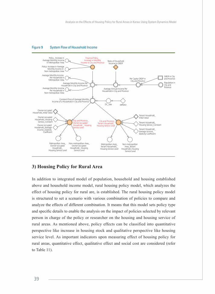
39


Figure 9 System Flow of Household Income

Policy_ Increase inAverage Monthly Income

in Metropolitan Area

Policy- Increase in Average Monthly Income in

Non-metropolitan Area

Average Monthly Income Per Household in

Metropolitan Area

Average Monthly IncomePer Household in

Non-metropolitan Area

Financial Policy_ Increase in Monthly

Income in City and ProvinceRatio of HouseholdIncome to GRDP

Average Annual Income PerHousehold in City and Province

Per Capita GRDP in City and Province

GRDP in City and Province

Population in City and Province

Average Monthly Income PerHousehold in City and Province

Constant Price of Average MonthlyIncome of a Household in City and Province

DC_rate

Owner-occupied Household_Initial Value

Owner-occupied Household_Housing

Service_Constant

Owner-occupied Household_Average

Income_Elasticity Coefficient

Metropolitan Area_Owner-occupied

Household_ Housing Service Level

Non-metropolitan Area_Owner-occupied

Household_ Housing Service Level

City and Province_Owner-occupied Household _ Housing Service Level

City and Province_Tenant Household_

Housing Service Level

Tenant Household_Initial Value

Tenant Household_ Housing Service_Constant

Tenant Household_ Average Income_Elasticity Coefficient

Non-metropolitan Area_Tenant

Household_Housing Service Level

Metropolitan Area_Tenant Household_ Housing Service Level

deflator

3) Housing Policy for Rural Area

In addition to integrated model of population, household and housing established above and household income model, rural housing policy model, which analyzes the effect of housing policy for rural are, is established. The rural housing policy model is structured to set a scenario with various combination of policies to compare and analyze the effects of different combination. It means that this model sets policy type and specific details to enable the analysis on the impact of policies selected by relevant person in charge of the policy or researcher on the housing and housing service of rural areas. As mentioned above, policy effects can be classified into quantitative perspective like increase in housing stock and qualitative perspective like housing service level. As important indicators upon measuring effect of housing policy for rural areas, quantitative effect, qualitative effect and social cost are considered (refer to Table 11).

40

Table 11 Indicator to Measure the Effects of Housing Policy for Rural Area

ClassificationMajor

IndicatorRelevant Variable Factor that Led to Policy Effect

Quantitative Effect

Housing Supply Rate

·Housing Stock·�The Number of Households

Increase in the housing supply rate by increasing housing stock through policy

The Number of Housing Units per 1,000 Persons

·Housing Stock·�Population

Increase in the number of housing units per 1,000 persons by increasing housing stock through policy

Qualitative Effect


·�Improvement of Housing Quality

Improvement in housing service level by improving the quality of housing through new housing supply and financial support for housing refurbishment and repair

·�Increase in Household Income

Improvement in housing service level by increasing household income indirectly through policy so that people can live in better housing environment

Social Cost

Financial Support

·The Number of Beneficiaries·�Financial Support Scale by

Policy

Social cost related to the government’s financial support to make policy effective

Loan Support·�The Number of Beneficiaries·�Loan Support Scale by Policy

Social cost related to the government’s loan support to make policy effective

Housing Price Support Amount

·�The Number of Beneficiaries·�The Ratio of Housing Price

Benefits

Social cost related to the housing price discount benefits to make policy effective

The policies subject to analysis include housing supply expansion policy, financial support for housing policy, loan support for housing policy and support for the stabilization of living. The system flow where individual policy exerts its influence is presented in Figure 10. For example, the housing supply target area is determined according to housing supply expansion policy and the total number of housing in the area will increase based on the determined number of new housing supply. In addition, if a household receives low-interest rate loan for housing purchase/rent/construction, the household can increase its income by the difference between market interest rate and low-interest rate supported by the government. If housing is supplied at the price lower than the market through policies like housing price ceiling system to stabilize housing

41


market, the households which purchase these houses can increase its incomes compared to the households which cannot buy the houses to which housing price ceiling system is applied. This household income increase can lead to improvement in housing service.

Under this system, Table 12 shows various combinations in housing policy scenario as input. For example, scenario can be established by setting the total number of housing, housing distributional ratio, target area, and timing of supply of rental housing and housing for sale. Therefore, the inputs in the rural housing policy evaluation model include the target and scope of policy including the number of houses to be constructed, the number of beneficiaries, financial support amount, application ratio and beneficial interest rate. The outputs in the model include quantitative indicators like housing supply rate and the number of housing units per 1,000 persons, and housing service level that represents the living standard of individual household.

Table 12 Definition of Input and Output in Housing Policy for Rural Area Model

Policy Input Output (Indicators of Major Expected Effects)

Housing Supply

Whether it is rental housing or housing for saleSupply areaSupply scale by regionSupply timing by region

Population size by region, housing supply rate, the number of households by occupancy type, housing service level

Support for Housing

Refurbishment and Repair

Whether it is direct refurbishment or loan with low interest rateIncome quantile of households subject to policy benefitLoan support scale per householdRatio of households that apply for the program

Housing quality, housing service level

Housing Financial Support

Whether it is loan for rental housing or housing for purchaseIncome quantile of households subject to policy benefitLoan support scale per householdRatio of households that apply for the program

Average household income by region, housing service level, household by occupancy type

Support for Housing

Stabilization

Whether it is housing allowance or rental housingIncome quantile of households subject to policy benefitSupport scale per household

Average household income by region, average income of households which receive minimum living allowance, housing service level of households which receive minimum living allowance

42

Figur

e 10

Sys

tem

Flow

of H

ousin

g Po

licy

Polic

y_Ci

ty a

nd P

rovin

ce-

Incr

ease

in R

enta

l Hou

sing

The

Ratio

of

Ren

tal

Hou

sing

Supp

ly

Supp

ort f

or N

ew C

onst

ruct

ion_

City

and

Pro

vince

_ N

umbe

r of

Incr

ease

in H

ousin

g

Supp

ort f

or N

ew

Cons

truct

ion_

City

_ N

umbe

r of

Incr

ease

in H

ousin

g

Hou

sing

Supp

ly:

Sale

and

Ren

tal

Hou

sing

Hou

sing

Supp

ly Ti

min

g_

Seou

l

Hou

sing

Stab

ilizat

ion_

City

and

Pro

vince

_In

crea

se in

Mon

thly

Inco

me

Nat

ionw

ide_

City

and

Pr

ovin

ce_

The

Num

ber o

f H

ouse

hold

s by

Inco

me

Brac

ket

Soci

al C

ost_

Nat

iona

l Pu

blic

Fin

anci

al

Supp

ort A

mou

ntN

atio

nal P

ublic

Fi

nanc

ial S

uppo

rt A

mou

nt fo

r the

Yea

r

Hou

sing

Pric

e Ce

iling_

City

and

Pro

vince

_In

crea

se in

Mon

thly

Inco

me

Hou

sing

Pric

e Ce

iling

Polic

yH

ousin

g Pr

ice

Ceilin

g_Ru

ral A

rea_

Incr

ease

in

Mon

thly

Inco

me

City

and

Pro

vince

_Rur

al A

rea_

Gen

eral

Hou

seho

lds

Supp

ly Po

licy_

Ratio

of R

ural

Are

a

Soci

al C

ost_

Rura

l Are

a_

Bene

fits

of H

ousin

g Se

lling

Pric

e

Soci

al C

ost_

Nat

ionw

ide_

Bene

fits

of H

ousin

g Se

lling

Pric

e

Nat

ionw

ide

Bene

fits

of

Hou

sing

Sellin

g Pr

ice

for t

he Y

ear

Bene

fits

of H

ousin

g Se

lling

Pric

e in

Rur

al A

rea

for t

he Y

ear

Hou

sing

Pric

e Ce

iling_

Rura

l Are

a_In

crea

se in

A

nnua

l Inc

ome

Hou

sing

Pric

e Ce

iling_

City

and

Pr

ovin

ce_I

ncre

ase

in A

nnua

l Inc

ome

Hou

sing

Pric

e Ce

iling_

City

and

Pro

vince

_ In

crea

se in

the

Inco

me

of T

hose

Who

Pur

chas

e a

Hou

se

City

and

Pro

vince

_ Av

erag

e Sa

le P

rice

of H

ousin

gSu

pply

Polic

y_Ci

ty a

nd

Prov

ince

_Num

ber o

f In

crea

se in

Hou

sing

Ratio

of B

enef

its o

f H

ousin

g Se

lling

Pric

e

City

and

Pro

vince

_G

ener

al H

ouse

hold

s

Hou

sing

Stab

ilizat

ion_

Inco

me

Qua

ntile

Hou

sing

Stab

ilizat

ion_

Bene

ficia

ry H

ouse

hold

Hou

sing

Stab

ilizat

ion

Supp

ort P

olic

y

Hou

sing

Stab

ilizat

ion_

Rura

l Are

a_In

crea

se in

Mon

thly

Inco

me

City

and

Pro

vince

_Ru

ral A

rea_

Gen

eral

H

ouse

hold

s

Rura

l Are

a_Ci

ty a

nd P

rovin

ce_

The

Num

ber o

f Hou

seho

lds

by In

com

e Br

acke

t

Fina

ncia

l Sup

port

Am

ount

fo

r Rur

al A

rea

for t

he Y

ear

Soci

al C

ost_

Pub

lic

Fina

ncia

l Sup

port

Am

ount

for R

ural

A

rea

Hou

sing

Stab

ilizat

ion_

Excl

udin

g O

wne

r-oc

cupi

ed H

ouse

hold

Nat

ionw

ide_

Ratio

of

Ow

ner-o

ccup

ied

Hou

seho

ld

Hou

sing

Supp

ly Ti

min

g_B

usan

Hou

sing

uppl

y Ti

min

g_D

aegu

Hou

sing

Supp

ly Ti

min

g_I

nche

onH

ousin

g Su

pply

Tim

ing

_Gw

angj

uH

ousin

g Su

pply

Tim

ing

_Dae

jeon

Hou

sing

Supp

ly Ti

min

g_U

lsan

Hou

sing

Supp

ly Ti

min

g_G

yeon

ggi

Hou

sing

Supp

ly Ti

min

g_G

angw

onH

ousin

g Su

pply

Tim

ing

_Chu

ngbu

kH

ousin

g Su

pply

Tim

ing

_Chu

ngna

mH

ousin

g Su

pply

Tim

ing

_Jeo

nbuk

Hou

sing

Supp

ly Ti

min

g_J

eonn

amH

ousin

g Su

pply

Tim

ing

_Gye

ongb

ukH

ousin

g Su

pply

Tim

ing

_Gye

ongn

amH

ousin

g Su

pply

Tim

ing

_Jej

u

Supp

ort f

or N

ew

Cons

truct

ion_

City

and

Pr

ovin

ce_N

umbe

r of

Incr

ease

in H

ousin

g

Supp

ort f

or N

ew

Cons

truct

ion_

Rura

l A

rea_

Num

ber o

f In

crea

se in

Hou

sing

Supp

ort f

or N

ew

Cons

truct

ion_

City

_N

umbe

r of

Incr

ease

in H

ousin

gSu

ppor

t for

New

Co

nstru

ctio

n_Ra

tio

of R

ural

Are

a

Capi

tal S

uppo

rt fo

r N

ew C

onst

ruct

ion

Polic

y

Num

ber o

f New

Cons

truct

ion_

Seo

ulN

umbe

r of N

ew C

onst

ruct

ion_

Bus

anN

umbe

r of N

ew C

onst

ruct

ion_

Dae

guN

umbe

r of N

ew C

onst

ruct

ion_

Inch

eon

Num

ber o

f New

Con

stru

ctio

n_ G

wan

gju

Num

ber o

f New

Con

stru

ctio

n_ D

aeje

onN

umbe

r of N

ew C

onst

ruct

ion_

Ulsa

nN

umbe

r of N

ew C

onst

ruct

ion_

Gye

ongg

iN

umbe

r of N

ew C

onst

ruct

ion_

Gan

gwon

Num

ber o

f New

Con

stru

ctio

n_ C

hung

buk

Supp

ort f

or N

ew C

onst

ruct

ion_

City

and

Pro

vince

_Inc

reas

e in

the

Num

ber o

f H

ousin

g

Capi

tal f

or N

ew C

onst

ruct

ion_

A

pplic

atio

n Ra

tio

Capi

tal f

or N

ew C

onst

ruct

ion_

Su

ppor

t Rat

io

Capi

tal f

or N

ew C

onst

ruct

ion_

Fa

vora

ble

Inte

rest

Rat

e

Capi

tal f

or N

ew

Cons

truct

ion_

City

and

Pro

vince

City

and

Pro

vince

_Av

erag

e Sa

le P

rice

of H

ousin

g

Supp

ort f

or N

ew

Cons

truct

ion

_Rat

io o

f Rur

al A

rea

Capi

tal f

or N

ew C

onst

ruct

ion

_Rur

al A

rea

Capi

tal f

or N

ew

Cons

truct

ion_

Nat

ionw

ide

Num

ber o

f New

Con

stru

ctio

n_ C

hung

nam

Num

ber o

f New

Con

stru

ctio

n_ Je

onbu

kN

umbe

r of N

ew C

onst

ruct

ion_

Jeon

nam

Num

ber o

f New

Con

stru

ctio

n_ G

yeon

gbuk

Num

ber o

f New

Con

stru

ctio

n_ G

yeon

gnam

Num

ber o

f New

Con

stru

ctio

n_ Je

ju

Tim

ing

of N

ew

Cons

truct

ion_

Seou

l

Capi

tal f

or N

ew

Cons

truct

ion_

Nat

ionw

ide

Nat

iona

l Fin

anci

al S

uppo

rtA

mou

nt fo

r the

Yea

r Soci

al C

ost_

Fin

anci

al

Supp

ort A

mou

nt

Nat

ionw

ide

Capi

tal S

uppo

rt fo

r Re

furb

ishm

ent P

olic

y

Refu

rbish

men

t_Ci

ty a

nd

Prov

ince

_ In

crea

se in

M

onth

ly In

com

e

Refu

rbish

men

t_Ci

ty a

nd

Prov

ince

_Inc

reas

e in

Ann

ual

Inco

me

Refu

rbish

men

t_Ci

ty a

nd

Prov

ince

_ In

com

e In

crea

se

by B

rack

et

Sum

of N

atio

nal S

uppo

rtfo

r Ref

urbi

shm

ent

Fina

ncia

l Sup

port

for H

ousin

gPu

rcha

se a

nd R

enta

l Hou

sing

Capi

tal S

uppo

rt_Ci

tyan

d Pr

ovin

ce_I

ncre

ase

in M

onth

ly In

com

e

Capi

tal S

uppo

rt_Ci

ty

and

Prov

ince

_Inc

reas

e in

Ann

ual I

ncom

e

Sum

of N

atio

nal

Capi

tal S

uppo

rt

City

and

Pro

vince

_ G

ener

al H

ouse

hold

s

Nat

ionw

ide_

City

and

Pr

ovin

ce_

The

Num

ber o

f H

ouse

hold

s by

Inco

me

Brac

ket

City

and

Pro

vince

_ Th

e N

umbe

r of H

ouse

hold

s by

Hou

sing

Serv

ice

Brac

ket

Capi

tal S

uppo

rt_

Incr

ease

in th

e In

com

eof

App

lican

ts

Capi

tal S

uppo

rt_

Favo

rabl

e In

tere

st R

ate

Capi

tal S

uppo

rt_

Inco

me

Qua

ntile

Capi

tal S

uppo

rt_

Supp

ort A

mou

nt

Capi

tal S

uppo

rt_Be

nefic

iary

Hou

seho

lds

Capi

tal S

uppo

rt_

Rura

l Are

a_

Inco

me

Incr

ease

by

Bra

cket

Capi

tal S

uppo

rt_Ru

ral A

rea_

Incr

ease

in A

nnua

l Inc

omeP

100

milli

on w

on/y

r

Capi

tal S

uppo

rt_Ru

ral A

rea_

Am

ount

of

Incr

ease

in

Mon

thly

Inco

me

Capi

tal S

uppo

rt fo

rH

ousin

g Pu

rcha

se a

ndRe

ntal

Hou

sing

Fina

ncia

l Sup

port

Am

ount

in R

ural

A

rea

for t

he Y

ear

Sum

of S

uppo

rtA

mou

nt fo

rRe

furb

ishm

ent

in R

ural

Are

a

Sum

of C

apita

l Su

ppor

t Am

ount

in

Rur

al A

rea

Soci

al C

ost_

Fina

ncia

lSu

ppor

t Am

ount

in R

ural

Are

a

Capi

tal S

uppo

rt fo

r Re

furb

ishm

ent P

olic

y

Refu

rbish

men

t_Ru

ral A

rea_

A

mou

nt o

f Inc

reas

e in

M

onth

ly In

com

e

Refu

rbish

men

t_Ru

ral A

rea_

In

crea

se in

Ann

ual I

ncom

e

Refu

rbish

men

t_Ru

ral A

rea_

In

com

e In

crea

se b

y Br

acke

t

Refu

rbish

men

t_Be

nefic

iary

Hou

seho

ldsRe

furb

ishm

ent_

Favo

rabl

e In

tere

st R

ate

Refu

rbish

men

t_In

com

e Q

uant

ileRe

furb

ishm

ent_

Supp

ort

Am

ount

Refu

rbish

men

t_A

pplic

atio

nRa

tio

Capi

tal S

uppo

rt_

App

licat

ion

Ratio Ru

ral A

rea_

The

Num

ber o

f H

ouse

hold

s by

Hou

sing

Serv

ice

Brac

ket

Rura

l Are

a_Ci

ty a

nd P

rovin

ce_

The

Num

ber o

f Hou

seho

lds

by In

com

e Br

acke

t

City

and

Pro

vince

_Rur

al A

rea_

G

ener

al H

ouse

hold

s

Tim

ing

of N

ew

Cons

truct

ion_

Busa

nTi

min

g of

New

Co

nstru

ctio

n_D

aegu

Tim

ing

of N

ew

Cons

truct

ion_

Inch

eon

Tim

ing

of N

ew

Cons

truct

ion_

Gw

angj

uTi

min

g of

New

Co

nstru

ctio

n_D

aeje

onTi

min

g of

New

Co

nstru

ctio

n_U

lsan

Tim

ing

of N

ew

Cons

truct

ion_

Gye

ongg

iTi

min

g of

New

Co

nstru

ctio

n_G

angw

onTi

min

g of

New

Co

nstru

ctio

n_Ch

ungb

ukTi

min

g of

New

Co

nstru

ctio

n_Ch

ungn

amTi

min

g of

New

Co

nstru

ctio

n_Je

onbu

kTi

min

g of

New

Co

nstru

ctio

n_Je

onna

mTi

min

g of

New

Co

nstru

ctio

n_G

yeon

gbuk

Tim

ing

of N

ew

Cons

truct

ion_

Gye

ongn

amTi

min

g of

New

Co

nstru

ctio

n_Je

ju

Polic

y_Ru

ral A

rea_

Num

ber o

f In

crea

se in

Ren

tal H

ousin

gPo

licy_

City

_Num

ber o

f In

crea

se in

Ren

tal H

ousin

g

Refu

rbish

men

t_Ci

ty a

nd P

rovin

ce_

Amou

nt o

f Inc

reas

ein

Mon

thly

Inco

me

Polic

y_ C

ity a

nd P

rovin

ce_

Am

ount

of I

ncre

ase

in M

onth

ly In

com

e

Polic

y_Ru

ral A

rea_

A

mou

nt o

f Inc

reas

e in

Mon

thly

Inco

me

Refu

rbish

men

t_ R

ural

A

rea_

Am

ount

of

Incr

ease

in M

onth

ly In

com

e

Capi

tal S

uppo

rt_ R

ural

A

rea_

Am

ount

of

Incr

ease

in M

onth

ly In

com

e

Hou

sing

Pric

e Ce

iling_

Ru

ral A

rea_

Am

ount

of

Incr

ease

in M

onth

ly In

com

e

Capi

tal S

uppo

rt_Ci

ty a

nd P

rovin

ce_

Amou

nt o

f Inc

reas

e in

Mon

thly

Inco

me

Hou

sing

Price

Cei

ling_

City

and

Pro

vince

_Am

ount

of I

ncre

ase

in M

onth

ly In

com

ePo

licy_

City

and

Pr

ovin

ce_I

ncre

ase

in G

ener

al H

ousin

g

Polic

y_Ru

ral A

rea_

N

umbe

r of I

ncre

ase

in G

ener

al H

ousin

g

Polic

y_Ci

ty_

N

umbe

r of I

ncre

ase

in G

ener

al H

ousin

g

Polic

y_Ci

ty a

ndPr

ovin

ce_

Am

ount

of

Incr

ease

in M

onth

lyIn

com

e of

Ten

ant

Hou

seho

ld

City

and

Pro

vince

_ Ra

tio o

f Ow

ner-o

ccup

ied

Hou

seho

ldPo

licy_

Rura

l Are

a_

Am

ount

of I

ncre

ase

in M

onth

ly In

com

e of

Ten

ant H

ouse

hold

Supp

ly Po

licy_

Rura

l Are

a_N

umbe

r of

Incr

ease

in H

ousin

g

Supp

ly Po

licy_

City

and

Pro

vince

_N

umbe

r of I

ncre

ase

in H

ousin

g

Supp

ly Po

licy_

City

_N

umbe

r of I

ncre

ase

in H

ousin

gSu

pply

Polic

y_Ra

tio

of N

ewly

Cons

truct

ed

Hou

sing

in R

ural

Are

a

Hou

sing

Supp

ly Po

licy:

City

and

Pro

vince

Hou

sing

Supp

ly Sc

ale

Hou

sing

Supp

ly Ti

min

g

Num

ber o

f Hou

sing

Cons

truct

ion:

Seo

ulN

umbe

r of H

ousin

g Co

nstru

ctio

n: B

usan

Num

ber o

f Hou

sing

Cons

truct

ion:

Dae

guN

umbe

r of H

ousin

g Co

nstru

ctio

n: In

cheo

nN

umbe

r of H

ousin

g Co

nstru

ctio

n: G

wan

gju

Num

ber o

f Hou

sing

Cons

truct

ion:

Dae

jeon

Num

ber o

f Hou

sing

Cons

truct

ion:

Ulsa

nN

umbe

r of H

ousin

g Co

nstru

ctio

n: G

yeon

ggi

Num

ber o

f Hou

sing

Cons

truct

ion:

Gan

gwon

Num

ber o

f Hou

sing

Cons

truct

ion:

Chu

ngbu

kN

umbe

r of H

ousin

g Co

nstru

ctio

n: C

hung

nam

Num

ber o

f Hou

sing

Cons

truct

ion:

Jeon

buk

Num

ber o

f Hou

sing

Cons

truct

ion:

Jeon

nam

Num

ber o

f Hou

sing

Cons

truct

ion:

Gye

ongb

ukN

umbe

r of H

ousin

g Co

nstru

ctio

n: G

yeon

gnam

Num

ber o

f Hou

sing

Cons

truct

ion:

Jeju

Hou

sing

Stab

ilizat

ion_

Excl

udin

g O

wne

r-occ

upie

d H

ouse

hold

City

and

Pro

vince

_G

ener

al H

ouse

hold

s

Hou

sing

Stab

ilizat

ion_

City

and

Pro

vince

_A

mou

nt o

f Inc

reas

e in

Av

erag

e M

onth

ly In

com

e

Hou

sing

Stab

ilizat

ion_

App

lican

ts_I

ncre

ase

in M

onth

ly In

com

e

Hou

sing

Stab

ilizat

ion_

Rura

l Are

a_In

crea

se in

M

onth

ly In

com

e

Finan

cial S

uppo

rt Po

licy

Hou

sing

Cons

truct

ion

in C

ity a

nd P

rovin

ce Scal

e of

Hou

sing

Cons

truct

ion

Tim

ing

of H

ousin

gCo

nstru

ctio

n

Hou

sing

Stab

ilizat

ion_

Supp

ort A

mou

nt

Hou

sing

Stab

ilizat

ion_

App

licat

ion

Ratio

Nat

ionw

ide_

Ann

ual

Publ

ic F

inan

cial

Sup

port

Am

ount

Hou

sing

Stab

ilizat

ion_

Rura

l Are

a_A

pplic

ants

_In

crea

se in

Mon

thly

Inco

me

Rura

l Are

a_Pu

blic

Fin

anci

al

Supp

ort A

mou

nt

43


Figur

e 10

Sys

tem

Flow

of H

ousin

g Po

licy

Polic

y_Ci

ty a

nd P

rovin

ce-

Incr

ease

in R

enta

l Hou

sing

The

Ratio

of

Ren

tal

Hou

sing

Supp

ly

Supp

ort f

or N

ew C

onst

ruct

ion_

City

and

Pro

vince

_ N

umbe

r of

Incr

ease

in H

ousin

g

Supp

ort f

or N

ew

Cons

truct

ion_

City

_ N

umbe

r of

Incr

ease

in H

ousin

g

Hou

sing

Supp

ly:

Sale

and

Ren

tal

Hou

sing

Hou

sing

Supp

ly Ti

min

g_

Seou

l

Hou

sing

Stab

ilizat

ion_

City

and

Pro

vince

_In

crea

se in

Mon

thly

Inco

me

Nat

ionw

ide_

City

and

Pr

ovin

ce_

The

Num

ber o

f H

ouse

hold

s by

Inco

me

Brac

ket

Soci

al C

ost_

Nat

iona

l Pu

blic

Fin

anci

al

Supp

ort A

mou

ntN

atio

nal P

ublic

Fi

nanc

ial S

uppo

rt A

mou

nt fo

r the

Yea

r

Hou

sing

Pric

e Ce

iling_

City

and

Pro

vince

_In

crea

se in

Mon

thly

Inco

me

Hou

sing

Pric

e Ce

iling

Polic

yH

ousin

g Pr

ice

Ceilin

g_Ru

ral A

rea_

Incr

ease

in

Mon

thly

Inco

me

City

and

Pro

vince

_Rur

al A

rea_

Gen

eral

Hou

seho

lds

Supp

ly Po

licy_

Ratio

of R

ural

Are

a

Soci

al C

ost_

Rura

l Are

a_

Bene

fits

of H

ousin

g Se

lling

Pric

e

Soci

al C

ost_

Nat

ionw

ide_

Bene

fits

of H

ousin

g Se

lling

Pric

e

Nat

ionw

ide

Bene

fits

of

Hou

sing

Sellin

g Pr

ice

for t

he Y

ear

Bene

fits

of H

ousin

g Se

lling

Pric

e in

Rur

al A

rea

for t

he Y

ear

Hou

sing

Pric

e Ce

iling_

Rura

l Are

a_In

crea

se in

A

nnua

l Inc

ome

Hou

sing

Pric

e Ce

iling_

City

and

Pr

ovin

ce_I

ncre

ase

in A

nnua

l Inc

ome

Hou

sing

Pric

e Ce

iling_

City

and

Pro

vince

_ In

crea

se in

the

Inco

me

of T

hose

Who

Pur

chas

e a

Hou

se

City

and

Pro

vince

_ Av

erag

e Sa

le P

rice

of H

ousin

gSu

pply

Polic

y_Ci

ty a

nd

Prov

ince

_Num

ber o

f In

crea

se in

Hou

sing

Ratio

of B

enef

its o

f H

ousin

g Se

lling

Pric

e

City

and

Pro

vince

_G

ener

al H

ouse

hold

s

Hou

sing

Stab

ilizat

ion_

Inco

me

Qua

ntile

Hou

sing

Stab

ilizat

ion_

Bene

ficia

ry H

ouse

hold

Hou

sing

Stab

ilizat

ion

Supp

ort P

olic

y

Hou

sing

Stab

ilizat

ion_

Rura

l Are

a_In

crea

se in

Mon

thly

Inco

me

City

and

Pro

vince

_Ru

ral A

rea_

Gen

eral

H

ouse

hold

s

Rura

l Are

a_Ci

ty a

nd P

rovin

ce_

The

Num

ber o

f Hou

seho

lds

by In

com

e Br

acke

t

Fina

ncia

l Sup

port

Am

ount

fo

r Rur

al A

rea

for t

he Y

ear

Soci

al C

ost_

Pub

lic

Fina

ncia

l Sup

port

Am

ount

for R

ural

A

rea

Hou

sing

Stab

ilizat

ion_

Excl

udin

g O

wne

r-oc

cupi

ed H

ouse

hold

Nat

ionw

ide_

Ratio

of

Ow

ner-o

ccup

ied

Hou

seho

ld

Hou

sing

Supp

ly Ti

min

g_B

usan

Hou

sing

uppl

y Ti

min

g_D

aegu

Hou

sing

Supp

ly Ti

min

g_I

nche

onH

ousin

g Su

pply

Tim

ing

_Gw

angj

uH

ousin

g Su

pply

Tim

ing

_Dae

jeon

Hou

sing

Supp

ly Ti

min

g_U

lsan

Hou

sing

Supp

ly Ti

min

g_G

yeon

ggi

Hou

sing

Supp

ly Ti

min

g_G

angw

onH

ousin

g Su

pply

Tim

ing

_Chu

ngbu

kH

ousin

g Su

pply

Tim

ing

_Chu

ngna

mH

ousin

g Su

pply

Tim

ing

_Jeo

nbuk

Hou

sing

Supp

ly Ti

min

g_J

eonn

amH

ousin

g Su

pply

Tim

ing

_Gye

ongb

ukH

ousin

g Su

pply

Tim

ing

_Gye

ongn

amH

ousin

g Su

pply

Tim

ing

_Jej

u

Supp

ort f

or N

ew

Cons

truct

ion_

City

and

Pr

ovin

ce_N

umbe

r of

Incr

ease

in H

ousin

g

Supp

ort f

or N

ew

Cons

truct

ion_

Rura

l A

rea_

Num

ber o

f In

crea

se in

Hou

sing

Supp

ort f

or N

ew

Cons

truct

ion_

City

_N

umbe

r of

Incr

ease

in H

ousin

gSu

ppor

t for

New

Co

nstru

ctio

n_Ra

tio

of R

ural

Are

a

Capi

tal S

uppo

rt fo

r N

ew C

onst

ruct

ion

Polic

y

Num

ber o

f New

Cons

truct

ion_

Seo

ulN

umbe

r of N

ew C

onst

ruct

ion_

Bus

anN

umbe

r of N

ew C

onst

ruct

ion_

Dae

guN

umbe

r of N

ew C

onst

ruct

ion_

Inch

eon

Num

ber o

f New

Con

stru

ctio

n_ G

wan

gju

Num

ber o

f New

Con

stru

ctio

n_ D

aeje

onN

umbe

r of N

ew C

onst

ruct

ion_

Ulsa

nN

umbe

r of N

ew C

onst

ruct

ion_

Gye

ongg

iN

umbe

r of N

ew C

onst

ruct

ion_

Gan

gwon

Num

ber o

f New

Con

stru

ctio

n_ C

hung

buk

Supp

ort f

or N

ew C

onst

ruct

ion_

City

and

Pro

vince

_Inc

reas

e in

the

Num

ber o

f H

ousin

g

Capi

tal f

or N

ew C

onst

ruct

ion_

A

pplic

atio

n Ra

tio

Capi

tal f

or N

ew C

onst

ruct

ion_

Su

ppor

t Rat

io

Capi

tal f

or N

ew C

onst

ruct

ion_

Fa

vora

ble

Inte

rest

Rat

e

Capi

tal f

or N

ew

Cons

truct

ion_

City

and

Pro

vince

City

and

Pro

vince

_Av

erag

e Sa

le P

rice

of H

ousin

g

Supp

ort f

or N

ew

Cons

truct

ion

_Rat

io o

f Rur

al A

rea

Capi

tal f

or N

ew C

onst

ruct

ion

_Rur

al A

rea

Capi

tal f

or N

ew

Cons

truct

ion_

Nat

ionw

ide

Num

ber o

f New

Con

stru

ctio

n_ C

hung

nam

Num

ber o

f New

Con

stru

ctio

n_ Je

onbu

kN

umbe

r of N

ew C

onst

ruct

ion_

Jeon

nam

Num

ber o

f New

Con

stru

ctio

n_ G

yeon

gbuk

Num

ber o

f New

Con

stru

ctio

n_ G

yeon

gnam

Num

ber o

f New

Con

stru

ctio

n_ Je

ju

Tim

ing

of N

ew

Cons

truct

ion_

Seou

l

Capi

tal f

or N

ew

Cons

truct

ion_

Nat

ionw

ide

Nat

iona

l Fin

anci

al S

uppo

rtA

mou

nt fo

r the

Yea

r Soci

al C

ost_

Fin

anci

al

Supp

ort A

mou

nt

Nat

ionw

ide

Capi

tal S

uppo

rt fo

r Re

furb

ishm

ent P

olic

y

Refu

rbish

men

t_Ci

ty a

nd

Prov

ince

_ In

crea

se in

M

onth

ly In

com

e

Refu

rbish

men

t_Ci

ty a

nd

Prov

ince

_Inc

reas

e in

Ann

ual

Inco

me

Refu

rbish

men

t_Ci

ty a

nd

Prov

ince

_ In

com

e In

crea

se

by B

rack

et

Sum

of N

atio

nal S

uppo

rtfo

r Ref

urbi

shm

ent

Fina

ncia

l Sup

port

for H

ousin

gPu

rcha

se a

nd R

enta

l Hou

sing

Capi

tal S

uppo

rt_Ci

tyan

d Pr

ovin

ce_I

ncre

ase

in M

onth

ly In

com

e

Capi

tal S

uppo

rt_Ci

ty

and

Prov

ince

_Inc

reas

e in

Ann

ual I

ncom

e

Sum

of N

atio

nal

Capi

tal S

uppo

rt

City

and

Pro

vince

_ G

ener

al H

ouse

hold

s

Nat

ionw

ide_

City

and

Pr

ovin

ce_

The

Num

ber o

f H

ouse

hold

s by

Inco

me

Brac

ket

City

and

Pro

vince

_ Th

e N

umbe

r of H

ouse

hold

s by

Hou

sing

Serv

ice

Brac

ket

Capi

tal S

uppo

rt_

Incr

ease

in th

e In

com

eof

App

lican

ts

Capi

tal S

uppo

rt_

Favo

rabl

e In

tere

st R

ate

Capi

tal S

uppo

rt_

Inco

me

Qua

ntile

Capi

tal S

uppo

rt_

Supp

ort A

mou

nt

Capi

tal S

uppo

rt_Be

nefic

iary

Hou

seho

lds

Capi

tal S

uppo

rt_

Rura

l Are

a_

Inco

me

Incr

ease

by

Bra

cket

Capi

tal S

uppo

rt_Ru

ral A

rea_

Incr

ease

in A

nnua

l Inc

omeP

100

milli

on w

on/y

r

Capi

tal S

uppo

rt_Ru

ral A

rea_

Am

ount

of

Incr

ease

in

Mon

thly

Inco

me

Capi

tal S

uppo

rt fo

rH

ousin

g Pu

rcha

se a

ndRe

ntal

Hou

sing

Fina

ncia

l Sup

port

Am

ount

in R

ural

A

rea

for t

he Y

ear

Sum

of S

uppo

rtA

mou

nt fo

rRe

furb

ishm

ent

in R

ural

Are

a

Sum

of C

apita

l Su

ppor

t Am

ount

in

Rur

al A

rea

Soci

al C

ost_

Fina

ncia

lSu

ppor

t Am

ount

in R

ural

Are

a

Capi

tal S

uppo

rt fo

r Re

furb

ishm

ent P

olic

y

Refu

rbish

men

t_Ru

ral A

rea_

A

mou

nt o

f Inc

reas

e in

M

onth

ly In

com

e

Refu

rbish

men

t_Ru

ral A

rea_

In

crea

se in

Ann

ual I

ncom

e

Refu

rbish

men

t_Ru

ral A

rea_

In

com

e In

crea

se b

y Br

acke

t

Refu

rbish

men

t_Be

nefic

iary

Hou

seho

ldsRe

furb

ishm

ent_

Favo

rabl

e In

tere

st R

ate

Refu

rbish

men

t_In

com

e Q

uant

ileRe

furb

ishm

ent_

Supp

ort

Am

ount

Refu

rbish

men

t_A

pplic

atio

nRa

tio

Capi

tal S

uppo

rt_

App

licat

ion

Ratio Ru

ral A

rea_

The

Num

ber o

f H

ouse

hold

s by

Hou

sing

Serv

ice

Brac

ket

Rura

l Are

a_Ci

ty a

nd P

rovin

ce_

The

Num

ber o

f Hou

seho

lds

by In

com

e Br

acke

t

City

and

Pro

vince

_Rur

al A

rea_

G

ener

al H

ouse

hold

s

Tim

ing

of N

ew

Cons

truct

ion_

Busa

nTi

min

g of

New

Co

nstru

ctio

n_D

aegu

Tim

ing

of N

ew

Cons

truct

ion_

Inch

eon

Tim

ing

of N

ew

Cons

truct

ion_

Gw

angj

uTi

min

g of

New

Co

nstru

ctio

n_D

aeje

onTi

min

g of

New

Co

nstru

ctio

n_U

lsan

Tim

ing

of N

ew

Cons

truct

ion_

Gye

ongg

iTi

min

g of

New

Co

nstru

ctio

n_G

angw

onTi

min

g of

New

Co

nstru

ctio

n_Ch

ungb

ukTi

min

g of

New

Co

nstru

ctio

n_Ch

ungn

amTi

min

g of

New

Co

nstru

ctio

n_Je

onbu

kTi

min

g of

New

Co

nstru

ctio

n_Je

onna

mTi

min

g of

New

Co

nstru

ctio

n_G

yeon

gbuk

Tim

ing

of N

ew

Cons

truct

ion_

Gye

ongn

amTi

min

g of

New

Co

nstru

ctio

n_Je

ju

Polic

y_Ru

ral A

rea_

Num

ber o

f In

crea

se in

Ren

tal H

ousin

gPo

licy_

City

_Num

ber o

f In

crea

se in

Ren

tal H

ousin

g

Refu

rbish

men

t_Ci

ty a

nd P

rovin

ce_

Amou

nt o

f Inc

reas

ein

Mon

thly

Inco

me

Polic

y_ C

ity a

nd P

rovin

ce_

Am

ount

of I

ncre

ase

in M

onth

ly In

com

e

Polic

y_Ru

ral A

rea_

A

mou

nt o

f Inc

reas

e in

Mon

thly

Inco

me

Refu

rbish

men

t_ R

ural

A

rea_

Am

ount

of

Incr

ease

in M

onth

ly In

com

e

Capi

tal S

uppo

rt_ R

ural

A

rea_

Am

ount

of

Incr

ease

in M

onth

ly In

com

e

Hou

sing

Pric

e Ce

iling_

Ru

ral A

rea_

Am

ount

of

Incr

ease

in M

onth

ly In

com

e

Capi

tal S

uppo

rt_Ci

ty a

nd P

rovin

ce_

Amou

nt o

f Inc

reas

e in

Mon

thly

Inco

me

Hou

sing

Price

Cei

ling_

City

and

Pro

vince

_Am

ount

of I

ncre

ase

in M

onth

ly In

com

ePo

licy_

City

and

Pr

ovin

ce_I

ncre

ase

in G

ener

al H

ousin

g

Polic

y_Ru

ral A

rea_

N

umbe

r of I

ncre

ase

in G

ener

al H

ousin

g

Polic

y_Ci

ty_

N

umbe

r of I

ncre

ase

in G

ener

al H

ousin

g

Polic

y_Ci

ty a

ndPr

ovin

ce_

Am

ount

of

Incr

ease

in M

onth

lyIn

com

e of

Ten

ant

Hou

seho

ld

City

and

Pro

vince

_ Ra

tio o

f Ow

ner-o

ccup

ied

Hou

seho

ldPo

licy_

Rura

l Are

a_

Am

ount

of I

ncre

ase

in M

onth

ly In

com

e of

Ten

ant H

ouse

hold

Supp

ly Po

licy_

Rura

l Are

a_N

umbe

r of

Incr

ease

in H

ousin

g

Supp

ly Po

licy_

City

and

Pro

vince

_N

umbe

r of I

ncre

ase

in H

ousin

g

Supp

ly Po

licy_

City

_N

umbe

r of I

ncre

ase

in H

ousin

gSu

pply

Polic

y_Ra

tio

of N

ewly

Cons

truct

ed

Hou

sing

in R

ural

Are

a

Hou

sing

Supp

ly Po

licy:

City

and

Pro

vince

Hou

sing

Supp

ly Sc

ale

Hou

sing

Supp

ly Ti

min

g

Num

ber o

f Hou

sing

Cons

truct

ion:

Seo

ulN

umbe

r of H

ousin

g Co

nstru

ctio

n: B

usan

Num

ber o

f Hou

sing

Cons

truct

ion:

Dae

guN

umbe

r of H

ousin

g Co

nstru

ctio

n: In

cheo

nN

umbe

r of H

ousin

g Co

nstru

ctio

n: G

wan

gju

Num

ber o

f Hou

sing

Cons

truct

ion:

Dae

jeon

Num

ber o

f Hou

sing

Cons

truct

ion:

Ulsa

nN

umbe

r of H

ousin

g Co

nstru

ctio

n: G

yeon

ggi

Num

ber o

f Hou

sing

Cons

truct

ion:

Gan

gwon

Num

ber o

f Hou

sing

Cons

truct

ion:

Chu

ngbu

kN

umbe

r of H

ousin

g Co

nstru

ctio

n: C

hung

nam

Num

ber o

f Hou

sing

Cons

truct

ion:

Jeon

buk

Num

ber o

f Hou

sing

Cons

truct

ion:

Jeon

nam

Num

ber o

f Hou

sing

Cons

truct

ion:

Gye

ongb

ukN

umbe

r of H

ousin

g Co

nstru

ctio

n: G

yeon

gnam

Num

ber o

f Hou

sing

Cons

truct

ion:

Jeju

Hou

sing

Stab

ilizat

ion_

Excl

udin

g O

wne

r-occ

upie

d H

ouse

hold

City

and

Pro

vince

_G

ener

al H

ouse

hold

s

Hou

sing

Stab

ilizat

ion_

City

and

Pro

vince

_A

mou

nt o

f Inc

reas

e in

Av

erag

e M

onth

ly In

com

e

Hou

sing

Stab

ilizat

ion_

App

lican

ts_I

ncre

ase

in M

onth

ly In

com

e

Hou

sing

Stab

ilizat

ion_

Rura

l Are

a_In

crea

se in

M

onth

ly In

com

e

Finan

cial S

uppo

rt Po

licy

Hou

sing

Cons

truct

ion

in C

ity a

nd P

rovin

ce Scal

e of

Hou

sing

Cons

truct

ion

Tim

ing

of H

ousin

gCo

nstru

ctio

n

Hou

sing

Stab

ilizat

ion_

Supp

ort A

mou

nt

Hou

sing

Stab

ilizat

ion_

App

licat

ion

Ratio

Nat

ionw

ide_

Ann

ual

Publ

ic F

inan

cial

Sup

port

Am

ount

Hou

sing

Stab

ilizat

ion_

Rura

l Are

a_A

pplic

ants

_In

crea

se in

Mon

thly

Inco

me

Rura

l Are

a_Pu

blic

Fin

anci

al

Supp

ort A

mou

nt

44

Integrated model of population, households and housing, household income model and rural housing policy model that analyzes the effects of rural housing policy are established. These three models are the ones that reflect the rural areas of Korea. If rural housing policy is implemented using the three models, market changes of rural housing and effects of policy can be shown. As shown in Figure 11, analysis model is composed of three integrated model of population, household, and housing, regional income and household income model, and rural housing policy model. There are 17 sub-models under them. If external inputs related with housing policy are added, existing population/household as well as regional and household income are changed and changes in population, household, housing, regional income and household income are forecast and social cost required to execute the policies, qualitative and quantitative policy effects are estimated. For example, in terms of quantitative policy effects, the housing supply rate and the number of housing units per 1,000 persons are calculated and in terms of qualitative effects, housing service level and social cost including financial support, loan support and support to lower housing price are calculated and presented.

Figure 11 Prospects for Future Housing Conditions in Rural Area and the Model Framework of the Policy Effect Analysis

Integrated Model of Population, Family and Housing

Model for Housing Market Forecasting and Policy Evaluation in Rural Area (ex)

Model of Regional and Household Income

DemographicModel by Age

Demographic Model by

Age Bracket

DemographicModel by Cityand Province

Household Modelwith Certain Characteristics

Household Model by House Type

Household Modelwith the Number of Members ina Household

Household Model with

Occupancy TypeModel of

VacantHome

Housing Model with General

Rental

Policy Type Support Type Support Target (ex)

Rental Housing/Housing for Sale

New Construction/Refurbishment/Rental

Support for Housing Cost

Housing PriceCeiling System

Rural Area

Households under Fourth Income Quantile

Households under Second Income Quantile

Households Which Purchased a Newly-Constructed House

2500 HousingUnits/yr

50 Million Won/Household

300,000 Won Per Month/ Household

-

-

30%

20%

5%

Housing SupplyExpansion Policy

Housing FinancialSupport Policy

Housing Allowance/Housing Voucher Policy

Housing MarketStabilization Policy

Support Scale(ex) Actual Benefit Ratio

Housing Model by Type

HousingModel with

Occupancy Type

Model ofHousing

Service Level

GRDP (Gross Regional Domestic

Product) Model

GDPModel

IndustrialModel

EmploymentModel

HouseholdIncomeModel

Effect of Rural Housing Policy

Quantitative Effect of Housing (housing supply rate, the number

of housing units per 1,000 persons)

Qualitative Effect of Housing (housing service level)

Social Cost (public financial support amount,

capital support amount, benefits of lower housing purchasing price)

Prospects for Rural Housing Market

Demographic Changes(population, demographic structure, aging,

economically active population, etc.)

Changes in Household(the number of households, single-person households, average number of members

in a household, etc.)

Changes in Housing (housing supply rate, the number

of housing units per 1,000 persons, vacant home ratio, etc.)

Changes in Regional and Household Income(industrial structure, regional income,

employment rate, household income, etc.)

Analysis on Policy Effects



46

In this chapter, effects of rural housing policies are compared and analyzed using integrated model of population, household, and housing, household income model, and rural housing policy model established above. Housing policy scenarios are established with variations and major indicators related to future housing are compared between the case with housing policy and case without housing policy to analyze policy effects.

Housing supply expansion measure, housing finance support measure, housing cost support measure to stabilize residence and housing price ceiling measure to stabilize housing market are put into the simulation. In terms of housing supply policies, the expansion of rental housing supply is assumed to look at policy effects and in terms of housing finance support policies, the financial support policy for housing purchase and rent and policy to provide loan at low interest rate for housing refurbishment and repair are analyzed. In terms of housing cost subsidy policies, the effects of application of housing allowance and housing voucher are analyzed. In lower-price housing supply policy through housing market stabilization, the effects of housing policy ceiling system are analyzed.

The basis year for the analysis is 2010 and the changes in housing service level in 2020 are compared and analyzed between the case where policy is executed and the case where policy is not executed.


47


1. Policy to Increase Supply for Rental Housing

The ratio of households which want long-term rental housing supply is high in low-income households and households with the elderly in rural areas. In general, most rental housing is supplied in the form of apartment so this type of supply is mainly used in urban areas. In case where the policy to expand rental housing in rural areas is used, the policy effects are analyzed. It is assumed that about 300,000 housing units are newly supplied every year under the master plan for housing supply2) and 20% of new housing units are provided to rural areas3). The allocation of new housing supply for each city and province is based on the share of households in 2010. In addition, the share of new housing supply for rural areas is simulated with 10%, 20% and 30% to compare policy effects.

It is estimated that housing service level of tenant households is improved by 0.03, 0.06, 0.07, and 0.08 when the ratio of new rental housing supply in rural areas is 10%, 20%, 30%, and 40% respectively as a result of housing supply measure (refer to Table 13).

The quantitative indicator changes show that if the status quo remains as it is without any additional policy implementation, the number of housing units per 1,000 persons in rural areas is 430 and that in the nation is 419 (refer to Table 14). Meanwhile, if the share of new housing supply in rural areas is assumed to be 20%, the number of housing units per 1,000 persons is 418 and 423 in rural areas and the whole nation respectively. If the share of new housing supply in rural areas is assumed to be 30%, and the share of rental housing is 20%, the number of housing units per 1,000 persons is 420 and 424 in rural areas and the whole nation respectively.

2) Assuming the supply amount planned in the most conservative way considering economic cycle changes

3) Based on the fact that the ratio of rural households in the nation is about 20% as of 2010.

48

Table 13 Effects of Rental Housing Supply Expansion Policy (based on 2020)


Basic Model10% Rental Housing

Supply20% Rental Housing

Supply30% Rental

Housing Supply

2010(A)

2020(B)

2020(C)

Policy Effects(C)-(B)

2020(D)

Policy Effects(D)-(B)

2020(E)

Policy Effects(E)-(B)

Rural Area_Owner-

occupied Household

92.63 99.71 99.99 0.28 99.94 0.23 99.88 0.17

Rural Area_Tenant

Household80.94 92.44 92.47 0.03 92.5 0.06 92.51 0.07

Nationwide_Owner-

occupied Household

100 109.35 111.5 2.15 111.05 1.7 110.65 1.3

Nationwide_Tenant

Household78.84 90.17 90.41 0.24 90.6 0.43 90.73 0.56

Table 14 Changes in Quantitative Indicator of Housing upon Expansion of Housing Supply in Rural Area

Housing Supply Rate in 2020

Basic Model Quantitative Indicator upon Ratio of Housing Supply in Rural Area

is 20% (2020)

Quantitative Indicator upon Ratio of Housing Supply in Rural Area

is 30% (2020)2010 2020

Rural Area 104.29 104.78 101.91 102.57

Nationwide 102.67 107.42 108.41 108.78

Rural Area_ the Number of Housing Units per

1,000 Persons395 430 418 420

Nationwide_ the Number of Housing

Units per 1,000 Persons366 419 423 424

Note 1) : Basic model shows quantitative indicator of housing in 2010 and 2020 assuming that the current status continues.

2) : Assuming that 300,000 houses are newly supplied every year and the share of rental housing is 20%.

49


2. Support for Housing Purchase and Cost on Rental House

The target and levels of benefits of policy should be assumed to compare the effects of the policy. The purpose of financial support including support for housing purchase and rental house is to stabilize the residence for households, which cannot afford to buy or rent a house on their own, so it is assumed that 2% interest discount is provided to households that belong to fifth income quantile or under. It is also assumed that about 10% of the target households apply for the support. The changes in housing service level are analyzed in case where support for housing purchase and rent is increased by 50 million to 200 million won. Table 15 presents the policy effects classifying the cases into the low-interest rate loan scale of 50 million, 100 million and 200 million won. Table 16 shows social costs to be required for each case. The most desirable policy may be the one that can improve housing service level by keeping social costs to the minimum. This model not only estimates the required spending but also designs policy combination executable with limited budget and estimates the housing service level improvement with the combination.

In case of tenant households in rural areas, housing service level is estimated to increase by 0.15 under the policy that provides 2% lower interest rate than market rate for 100 million won support for housing purchase or rent and social costs to execute the policy are estimated to be 52.6 billion won in rural areas.

In case of tenant households in rural areas, if the financial support amount increases by 100 million won to 200 million won, housing service level is estimated to increase by 0.29 under the policy that provides 2% lower interest rate than market rate and social costs to execute the policy are estimated to be 105.2 billion won in rural areas.

50

Table 15 Policy Effects of Supporting Low-Interest Rate for Housing Purchase Loan (based on 2020)

Housing Service

Indicator

Basic Model50 Million Won

Loan100 Million Won

Loan200 Million Won

Loan

2010(A)

2020(B)

2020(C)

Policy Effects(C)-(B)

2020(D)

Policy Effects(D)-(B)

2020(E)

Policy Effects(E)-(B)

Rural Area_ Owner-

occupied92.63 99.71 99.76 0.05 99.8 0.09 99.89 0.18

Rural Area_ Tenant

80.94 92.44 92.51 0.07 92.59 0.15 92.73 0.29

Nationwide_ Owner-

occupied100 109.35 109.39 0.04 109.43 0.08 109.51 0.16

Nationwide_Tenant

78.84 90.17 90.22 0.05 90.27 0.1 90.37 0.2

Note 1): The housing service level of owner-occupied household in the nation as of 2010 is 100 2): It shows housing service level in 2020 in case of financial support for housing purchase or rent every

year by 2020 3): (A) and (B) show housing service level without any policy implementation. 4): Policy effects are shown by comparing the housing service level in 2020 without any policy

implementation and housing service level in 2020 with policy implementation.

Table 16 Social Cost Estimate upon Support for Low-Interest Rate for Housing Purchase Loan

(Unit: 100 million won/every year)

Support Amountper Household 50 Million Won 100 Million Won 200 Million Won

Rural Area 262.9 526.0 1,052.0

Nationwide 1,057.4 2,115.1 4,230.3

51


3. Effects of Low-Interest Rate Loan (Support for Expenses on Refurbishment and Repair)

In rural areas, the demand for housing refurbishment and repair is high as houses are very old. The target of support for housing refurbishment and repair can be established as low income households that belong to third income quantile or under and it can be expanded to compare the case with the one where the policy is applied to households that are supported by low-interest loan for purchase and rent. Low-interest rate loan for housing refurbishment and repair is assumed to be provided to households that belong to third household income quantile and fifth household income quantile with 2% interest rate discount. It is also assumed that about 10% of the target households apply for the benefits.

In case where 100 million won loan is provided with low interest rate for housing refurbishment and repair to those that belong to third household income quantile, housing service indicator increased by 0.1 for owner-occupied households and 0.2 for tenant households in rural areas respectively (refer to Table 17). In this case, the social cost is estimated that 74.8 billion won is required annually.

Meanwhile, if the 200 million won loan with low interest rate is provided to those under fifth income quantile for housing refurbishment and repair, housing service indicator increased by 0.9 for owner-occupied households and 1.5 for tenant households in rural areas respectively. In this case, the social cost is estimated that 526 billion won is required annually.

52

Table 17 Policy Effect of Supporting Low-Interest Rate Loan for Housing Refurbishment and Repair (based on 2020)

Scenario

2010 2020 Required Budget

Estimate(Social cost)

Owner-occupied

TenantOwner-

occupiedTenant

Scenario1

Third income quantile/100 million won loan/household

application rate of 20%

92.82 81.24 99.83 92.64

74.8 Billion Won

Basic Model 92.63 80.94 99.71 92.44

Policy Effect 0.1 0.2 0.1 0.1

Scenario2

Fifth income quantile/200 million won loan/ household

application rate of 50%

93.98 88.07 100.58 93.89

526 Billion Won

Basic Model 92.63 80.94 99.71 92.44

Policy Effect 1.2 1.3 0.5 0.5

4. Effects of Housing Allowance / Housing Voucher System

Housing allowance and housing voucher system is intended to provide residence cost to the lessee to stabilize the residence for the households with lowest income and worst housing condition. The changes in housing service level and required budget are estimated in case where the housing allowance or housing voucher policy is used.

It is assumed that 300,000 won are provided on a monthly basis to households that belong to second income quantile or under regardless of occupancy type and 90% of those households apply for the system, the housing service indicator increased by 1.21 and 0.73 for tenant households and owner-occupied households in rural areas respectively. It is estimated that every year, 448.57 billion won is required in rural areas as social cost (refer to Table 18).

53


It is assumed that 300,000 won are provided on a monthly basis to households that do not own housing and belong to the second income quantile or under and 90% of those households apply for the system, the housing service indicator increased by 0.47 for tenant households in rural areas. It is estimated that every year 208.57 billion won is required as social cost in rural areas

Table 18 Effect of Housing Allowance/Housing Voucher Policy


Basic ModelSecond Income Quantile

Households

Second Income Quantile Households (Only for household without

housing)

2010(A)

2020(B)

2020(C)

Policy Effect(C)-(B)

2020(D)

Policy Effect(D)-(B)

Rural Area_ Owner-occupied

92.63 99.71 100.44 0.73 99.71 0

Rural Area- Tenant

80.94 92.44 93.65 1.21 92.91 0.47

Nationwide_Owner-occupied

100 109.35 109.87 0.52 109.35 0

Nationwide_ Tenant

78.84 90.17 90.81 0.64 0.25 0.49

Annual Budget to be Required

(Social cost)- 448.57 Billion Won 208.57 Billion Won

54

5. Housing Market Stabilization Policy: Application of Housing Price Ceiling System

Housing price ceiling system is used as a means to control housing price by the government to provide housing at lower cost. Using the system, the policy effects of providing new houses at the cost lower than market price are analyzed. Assuming that 300,000 houses are newly supplied every year4) and housing price ceiling system is implemented to provide houses at the price lower than market price, it is necessary to review the housing service level changes in rural areas before executing policy. Therefore, policy effects are reviewed by changing the discount rate of housing price ceiling system to 10%, 20% and 30%.

It is estimated that houses are provided at lower cost by applying 10% discount of housing price ceiling, housing service level increased by 0.26 and 0.11 for owner-occupied households and tenant households in rural areas respectively. It is estimated that houses are provided at lower cost by applying 20% discount of housing price ceiling, housing service level increased by 0.29 and 0.17 for owner-occupied households and tenant households in rural areas respectively. It is estimated that houses are provided at lower cost by applying 30% discount of housing price ceiling, housing service level increased by 0.33 and 0.23 for owner-occupied households and tenant households in rural areas respectively (refer to Table 19).

Table 19 Effect of Expanding the Discount of Housing Price Ceiling System (based on 2020)

Housing Service

Indicator

Basic Model 10% Discount 20% Discount 30% Discount

2010

(A)

2020

(B)

2020

(C)

Policy

Effects

(C)-(B)

2020

(D)

Policy

Effects

(D)-(B)

2020

(E)

Policy

Effects

(E)-(B)

Rural Area_ Owner-

occupied92.63 99.71 99.97 0.26 100 0.29 100.04 0.33

Rural Area_Tenant 80.94 92.44 92.55 0.11 92.61 0.17 92.67 0.23

Nationwide_Owner-

occupied100 109.35 111.07 1.72 111.1 1.75 111.12 1.77

Nationwide_Tenant 78.84 90.17 90.63 0.46 90.66 0.49 90.68 0.51

4) Assuming the supply amount planned in the most conservative way considering economic cycle changes

55


6. Overall Comparative Analysis on Policy Effects

Each policy program has its own purpose so the timing and level of implementation should be determined based on the purpose. However, the improvement of housing and relevant social cost should be reviewed for each policy program before implementing policy. By doing so, the budget on housing policy can be allocated more efficiently. According to the analysis result (refer to Table 20), the most effective policy to improve the housing service levels of tenant households in rural areas is to support for housing purchase and rent followed by housing allowance and housing voucher system targeting households that belong to second income quantile. Meanwhile, as the expansion of long-term rental housing supply and affordable housing supply cause lots of social costs, the policy effects are not significant.

If only policy effects are considered without the consideration of social cost, the most effective policy is to support 300,000 won per month to households that belong to second income quantile or under. The second most effective policy is to support 300,000 won per month to households without housing that belong to second income quantile or under. The third most effective policy is to supply houses at price 20% lower than market price.

There is significant difference between the case considering both costs and effects and the case considering only policy effects. As the basic financial resources for housing policy are coming from tax, the budget should be allocated efficiently, and policy effects should be thoroughly reviewed before implementing policies.

56

Table 20 Comparative Analysis on Housing Service Level Improvement Compared to Social Cost for Each Policy

Housing

Service

Indicator

Policy

Social

Cost

(100

million

won)

Rural Area_Owner-

occupied HouseholdRural Area_ Tenant

Policy

Effects

Policy Effects/

Social Cost for

Owner-occupied

Household in

Rural Area

Policy

Effects

Policy Effects/

Social Cost for

Tenant in Rural

Area

Financial

Support

100 Million Won

Loan, 2%

Favorable

Interest Rate

526 0.09 0.00024 0.15 0.00098

Long-term

Rental

Housing

Supply

10% Expansion 4,104 0.28 9.61E-05 0.03 2.52E-05

20% Expansion 8,208 0.23 3.95E-05 0.06 2.52E-05

Housing

Supply

at Lower

Cost

10% Discount 4,560 0.26 8.03E-05 0.11 8.32E-05

20% Discount 9,120 0.29 4.48E-05 0.17 6.43E-05

Housing

Allowance/

Housing

Voucher

300,000 Won

(second income

quantile or under)

4,486 0.73 0.00023 1.21 0.00093

300,000 Won

(second income

quantile or

under/without

housing)

2,086 - - 0.47 0.00023

Note 1): It is assumed that among new supply of 300,000 houses, the ratio of rental housing increases by 10 to 30% and the ratio of rural households is 19% as of 2010.

2): The construction price for permanent rental housing is assumed to be 72 million won per unit (as of 2012).

3): Assuming that housing supply at lower cost means every year 300,000 new housing units are supplied at price 10 to 20% lower than new housing price (based on 2010 Korea housing survey, average price of rural housing is 80 million won).

4): Policy effects are accounted for by changes of housing service level in 2020 if policy is implemented 5): Policy effects and social costs are estimated by allocating social costs to owner-occupied household

and tenant considering the share of each in rural households.


Conclusion

58

In Korea, rural areas have long been an important basis for living. However, the status of rural areas has been weakened with a rapid decrease in population and households in rural areas and inflow of population into cities due to urbanization and industrialization. Many problems have occurred in rural areas including worn-out houses or vacant homes. In the meantime, new trend of returning to farming and rural areas has emerged as many people want to live in nature after retirement or people want to live a brand new life in rural areas. Now is the time to review the housing conditions and environment in rural areas to make the areas more livable place for many people.

In quantitative terms, the housing conditions in rural areas are good with appropriate number of houses, but the ratio of vacant home is high, which serves as a major factor in deteriorating living environment. In qualitative terms, the issues of safety and convenience emerge as there are many old and rundown houses. In addition, the possibility of refurbishing or repairing the houses is low as most residents in the house are the elderly.

This study defines rural areas as administrative districts classified into town and township and rural housing as the house located in rural areas. The purpose of this study is to analyze the effects of housing policy on rural areas and identify the most effective policy. To this end, “housing service indicator”, which shows qualitative conditions of housing, was developed along with quantitative indicator on housing and living conditions. In addition, a simulation model was developed using system dynamics (SD) by identifying causal relationship among various elements that compose the rural society. Based on the model, this study forecasts future housing

Conclusion

59


conditions in rural areas and measures effects of housing policies to compare policy programs designed to improve housing conditions in rural areas.

The development of SD model to analyze the effects of housing policy for rural areas is a huge task. 7 processes are required to develop the model: designing various sub-models that compose the society, identifying causal relationship among variables in individual sub-model and system flow, establishing model, analyzing the behavior in model, evaluating the feasibility, analyzing policy and making a decision. Population Housing Integration Model, Regional Income and Household Income Model and Housing Policy Model were established as a big model and 17 sub-models were established under them. Based on the model, a future housing market in rural areas was expected and policy effects including quantitative effects like housing supply rate and the number of housing units per 1000 persons, and qualitative effects like housing conditions and required financial resources to implement the policy were estimated.

Policy effects against costs were compared and analyzed using SD model and the result shows that the policies that could lead to the most significant improvement in housing conditions for tenant households in rural areas are policies that support housing purchase and fund for rent followed by housing allowance and housing voucher system, which are living cost subsidy system designed for households that belong to second income quantile or lower. It is found that policies that regulate the price of housing supply price like expansion of long-term rental housing supply and housing price ceiling system through market stabilization incur significant social costs led by construction while effects are not significant.

The academic achievement of this study is the making of “housing condition indicator”, which shows the quality of housing conditions. The housing service level indicator can show housing quality of individual housing as well as compare relative housing service levels by region and time to analyze policy effects compared to the case using proxy variables to identify quality of housing (the ratio of households that do not meet the minimum housing standard, ratio of vacant home, etc). It is meaningful in that the housing service level for individual housing is developed for the first time. In addition, the model which enables estimation of future rural housing and housing conditions using SD is developed. Existing studies showed limitation to establish and analyze model on rural housing conditions. In this regard, it can be said that this study opens a new chapter for rural housing policy research.

60

Reference

Jung Il-hong et al. 2010. “Characteristics of Urban Citizens Moving to Rural Area and Their Preference”, Rural Society, Vol. 20, No.2 pp.163-190.

Kang Mi-na et al. 2012. “A Rural Housing Policy for Improving Housing Service level.” Gyeonggi : Korea Research Institute for Human Settlements

Kim Do-hoon et al. 1999. 「System Dynamics」. Daeyoung Publication.Kim Hyung-yong. 1998. “Study on the State of Those Returning to Rural Area and

Ways for Their Settlement”, ” Korean Journal of Livestock Management. Vol. 14 No.1 pp.205~223. Korea Association of Livestock Management.

Kim Jung-ho. 2005. “Current State of Rural Housing and Policy Implications”. Korea Local Government Review. Vol. 7 No.2. pp. 71-89.

Kim Young-pyo. 2009. “System Dynamics Method”. pp.385~400. 「Easy to Understand National Land Research Method」. Gyeonggi : Korea Research Institute for Human Settlements

Lee Hae-wook. 2009. “Study on the Direction of Rural Housing Planning through Analysis on Rural Residence Type”. Rural Planning, Vol.15, No.2 pp.43-57.

Ministry of Agriculture, Food and Rural AffairsㆍKorea Rural Community Corporation. 2008. 「Study on the Development of Survey Structure and Method for Housing State in Rural Area」.

Ministry of Agriculture, Food and Rural AffairsㆍKorea Rural Community Corporation. 2010. 「Study on the Development of Desirable Rural and Fishing Area Development Model for 30 Years from Now」.

Ministry of Land, Infrastructure and Transport. 2011. 「Handbook on Work related to Housing」.Nah Gun-woo. 2002. Study on the State of Empty House in Rural Area and How to

Use It- Focusing on Geumsan-gun Area-Graduate School of Science and Industry Education, Joongbu University, Paper for Master’s Degree.

Song Mi-ryung et al. 2009. 「Trend and Implication of Rural Policy in Other Countries」Seoul : Korea Rural Economic Institute

Statistics Korea, Estimate on Future Population and HouseholdsStatistics Korea, Survey on Farming and Fishing Villages, 2005-2010Statistics Korea, Survey on Population and Housing, 2005-2010Yoon Hee-jung. 2011 “Establishment of Criteria for Minimum Housing Standard in

Town and Township and Guideline” Rural Planning Vol.17 No. 2 pp.13-21.

analysis on the effects of housing policy for rural areas

Documents