analysis of unit-magnitude constrained phasor reconstruction problems

1412 J. Opt. Soc. Am. A/Vol. 14, No. 7 /July 1997 Roque Kwok-Hung Szeto

Analysis of unit-magnitude constrained phasorreconstruction problems

Roque Kwok-Hung Szeto

Earth Resources Laboratory, Massachusetts Institute of Technology, 42 Carleton Street,Cambridge, Massachusetts 02142-1324

Received September 19, 1996; revised manuscript received January 10, 1997; accepted February 4, 1997

Many physical problems in adaptive optics and imaging application result in the optimization of a Hermitianform, xTHx, where H is an (n 3 n) Hermitian matrix and x is an n-component complex vector whose ele-ments are constrained to have unit magnitude. In this work the technique of Lagrange multiplers is used toderive the governing nonlinear equations. An efficient numerical algorithm is constructed to solve the non-linear equations. Of particular interest are applications that admit of nonunique solutions (e.g., problemsarising from phase difference measurements). Newton’s method is applied to an inflated system of equations.This significantly improves the region inside which Newton’s method converges quadratically. A practicalexample of phasor reconstruction from phase difference measurements is given to illustrate the developedtheory. In the example it is shown how the Lagrange multipliers can be used to give an a posteriori estimateof the measurement noise. For general Hermitian matrices, practical considerations of the developed algo-rithm are discussed. © 1997 Optical Society of America [S0740-3232(97)02807-X]

Key words: adaptive optics, phasor reconstruction, Hermitian-form optimization.

1. INTRODUCTIONThe method of Lagrange multipliers is often used to solveconstrained optimization problems,1 with the resultingnonlinear equations solved by Newton’s method. Inmany applications in adaptive optics and imagingthrough the atmosphere, the problems can be formulatedas a unit-magnitude phasor optimization of a Hermitianform. In the work presented here a general theory is de-veloped and an efficient algorithm is given for this type ofconstrained optimization problem.For applications that are concerned with phase differ-

ence measurements, it is well known that a constantphase, also known as a piston, is an unobservable mode inthe reconstruction of the unknown phase f (r) from phasedifference measurements. That is, the solution is uniqueup to an additive constant: f(r) 1 p is a solution forany arbitrary constant p. In terms of reconstruction ofphasors, x(r), from phase difference measurements, thesolution is unique up to a multiplicative constant of theform exp(ia), where a is an arbitrary real number:x(r)exp(ia) is also a solution for any arbitrary real num-ber a.The significance of nonunique solutions is that the

Jacobian matrix (Frechet derivative) of the set of nonlin-ear equations is singular evaluated at the solution,@x* (r), l* #, where l denotes the vector containing theLagrange multipliers. It is known2,3 that Newton’smethod for singular Jacobian matrices converges inside acone that is generally smaller than the region if the Jaco-bian matrix is nonsingular and that for most singularJacobian matrices the convergence rate is only linear. Inthis work the system of equations is inflated by requiringthat the solution be piston free: that is, the constrainedsolution is geometrically isolated. The condition inwhich the Jacobian matrix of the inflated system is non-

0740-3232/97/0701412-09$10.00 ©

singular is given. An efficient numerical algorithm is de-veloped to solve the inflated system of equations.The work presented here is divided into three parts.

In Section 2 the general theory is presented. A simpleexample of phasor reconstruction from phase differencemeasurements is illustrated in Section 3: it is generallywell known that linear least-squares phase reconstruc-tion from phase difference measurements4–7 does notwork well for adaptive optics correction for moderate tohigh atmospheric turbulence scintillation levels8,9 be-cause of the presence of branch points that occur at nullintensity values. Practical considerations are discussedin Section 4.

2. THEORY OF UNIT-MAGNITUDECONSTRAINED OPTIMIZATION OFHERMITIAN FORMThe optimization problem can be formulated as

maxx

xTHx, (1)

where x is an n-component complex vector, H is a Her-mitian matrix, and the overbar denotes complex-conjugate operation. The optimization is solved subjectto the n constraints that the n components of x have unitmagnitude,

uxiu2 5 1, i 5 1, ..., n. (2)

The most common method for the constrained optimiza-tion problem is the use of Lagrange multipliers. For then constraints in Eq. (2) we introduce n Lagrange multi-pliers, l j , j 5 1, ..., n. We next note that in many adap-tive optics applications, as with phase reconstructionfrom phase difference measurements, the piston is an un-observable mode, [or, correspondingly in phasor terms,

1997 Optical Society of America

Roque Kwok-Hung Szeto Vol. 14, No. 7 /July 1997 /J. Opt. Soc. Am. A 1413

the solution vector u 1 iv is determined up to a multipli-cative constant exp(ia), for any real constant a]. An ad-ditional constraint is needed to isolate a unique solution:the simple constraint that the sum of the imaginary partsof the components of x vanish is imposed,

(i51

n

I xi 5 0. (3)

The constraint in Eq. (3) can be interpreted as the zeroaverage phase constraint. To see this, we consider n ar-bitrary unit-magnitude phasors. Then we define the av-erage phase fp in accordance with the equation,

fp 5 tan21~Y/X !, (4)

where X and Y are the average of the real and the imagi-nary parts, respectively, of the n phasors:

X 51

n (i51

n

Rxi , (5)

Y 51

n (i51

n

I xi . (6)

From Eq. (4) the average phase fp is zero if the value ofY is zero. We see that from Eq. (6) this is equivalent tothe constraint in Eq. (3). We further note that to removethe average phase from the n complex unit-magnitudephasors xi , we multiply xi by exp(2ifp). It is trivial toshow that the resulting product xi exp(2ifp) has zero av-erage phase by proving that the imaginary part of thesum of the n average phase removed phasors vanishes:

1

n (i51

n

xi exp~2ifp! 5 ~X2 1 Y2!1/2. (7)

In addition to the n Lagrange multipliers, l i , i5 1, ..., n for the n constraints in Eq. (2), we introducean additional Lagrange multipler, m8, for the zero aver-age phase constraint in Eq. (3) and rewrite the unit-magnitude constrained Hermitian-form optimizationproblem as

maxx,l,m

xTHx 1 lTc 1 m81TI x, (8)

where c is an n-component vector containing the unit-magnitude phasor constraints in Eq. (2),

c 5 ~ ux1u2 2 1, ux2u2 2 1, ..., uxiu2 2 1, ... !T, (9)

and 1 is an n-component vector whose entries are all 1’s.The functional to be maximized is an inherent real quan-tity. It is useful at this point to introduce the notation uand v to denote the real and the imaginary parts of x, re-spectively. We also introduce the symmetric matrix Aand the skew-symmetric matrix B to be the real part andimaginary part of H in Eq. (1). That is,

u 5 Rx, (10)

v 5 I x, (11)

A 5 RH, (12)

B 5 IH. (13)

Substituting Eqs. (10)–(13) into Eq. (8), we obtain the re-sult

maxx,l,m8

xTHx 1 lTc 1 m81TI x

5 maxu,v,l,m8

@uT~Au 2 Bv! 1 vT~Av 1 Bu!

1 lTc~u , v! 1 m81Tv]. (14)

The problem now becomes a simple unconstrained optimi-zation problem of finding a solution for u, v, l and m8 thatmaximizes the functional W(u, v, l, m8),

W~u, v, l, m8! [ uT~Au 2 Bv! 1 vT~Av 1 Bu!

1 lTc~u,v! 1 m81Tv. (15)

To proceed we take derivatives with respect to uT, vT,lT, and m8 and set the resulting expressions to zero,

Au 2 Bv 5 2Lu, (16)

Av 1 Bu 5 2Lv 2 m1, (17)

Uu 1 Vv 5 1, (18)

1Tv 5 0, (19)

where matrices U, V, and L are diagonal matrices whoseelements are the variables, ui , vi , and l i , respectively,

U 5 diag~u1 , u2 , ... !, (20)

V 5 diag~v1 , v2 , ... !, (21)

L 5 diag~l1 , l2 , ... !, (22)

and m is related to m8 in accordance with the equation,

m 512 m8. (23)

In passing, the following equation will be needed in theanalysis of the Lagrange multipliers. We multiply Eq.(17) by i, add the resulting equation to Eq. (16), and withuse of the relations in Eqs. (10)–(13),

Hx 5 2Lx 2 im1. (24)

There are many iterative methods available in the so-lution of the set of nonlinear equations in Eqs. (16)–(19).If the associated Jacobian matrix is banded and nonsin-gular and if an initial-guess vector (u0, v0, l0, m0)T isreadily available, then Newton’s method is one of themost efficient methods because of the nature of the qua-dratic rate of convergence. The additional constraint asgiven by Eq. (3) forces the inflated system of equations tohave a geometrically isolated solution. For reasons thatwill become clear later in this section, the Jacobian ma-trix for the inflated system is nonsingular if the nontrivialsolution of the equations,


F A 1 L~l* ! B U~u* !

2B A 1 L~l* ! V~v* !

U~u* ! V~v* ! 0G S cr

ci

cl

D 5 0, (25)

F A 1 L~l* ! 2B U~u* !

B A 1 L~l* ! V~v* !

U~u* ! V~v* ! 0G S fr

fi

fl

D 5 0, (26)

satisfies the inequalities,

1Tci Þ 0, (27)

1Tfi Þ 0. (28)

We next recognize that for most adaptive optics and im-aging applications the matrices A and B on the left-handside of Eqs. (25) and (26) are functions of the phase dif-ference measurements only; therefore the inner products1Tci and 1Tfi are almost never zero. That is, the Jaco-bian matrix for the inflated system is almost always non-singular. We can conclude that Newton’s method whenapplied to the inflated system will converge quadraticallyalmost all the time provided that a good initial guess canbe found to lie within the ball of convergence. Thereforewe shall restrict our discussion of the method of solutionof Eqs. (16)–(19) to the use of Newton’s method.We let (un, vn, ln, mn) be some iterate sufficiently close

to the solution of Eqs. (16)–(19). Then Newton’s methodcan be described by the equations,

~A 1 Ln!dun 2 Bdvn 1 Undln 5 2d f1n , (29)

Bdun 1 ~A 1 Ln!dvn 1 Vndln 1 dmn1 5 2d f2n , (30)

2Undun 1 2Vndvn 5 2d f3n , (31)

1Tdvn 5 2d f4n , (32)

where dfin , i 5 1, ..., 4 are the residuals at the n th itera-

tion:

df1n 5 Aun 2 Bvn 1 Lnun, (33)

df2n 5 Bun 1 Avn 1 Lnvn 1 mn1, (34)

df3n 5 Unun 1 Vnvn 2 1, (35)

df4n 5 1Tvn. (36)

The (n 1 1)st iterates are given by the equations,

un11 5 un 1 dun, (37)

vn11 5 vn 1 dvn, (38)

ln11 5 lm 1 dln, (39)

mn11 5 mn 1 dmn. (40)

There are altogether (3n 1 1) linear scalar equations inthe four matrix equations (29)–(32) for the (3n 1 1) un-knowns: the three n-component vectors dun, dvn, dln

and the additional Lagrange multiplier dmn. We nextuse the properties of the unit-magnitude constraints that

U and V be diagonal matrices to simplify the (3n 1 1)equations, Eqs. (29)–(32), to just (n 1 1) linear scalarequations.To proceed, we multiply Eq. (30) by i and add the re-

sulting equation to Eq. (29):

~A 1 iB 1 Ln!~dun 1 idvn! 1 ~Un 1 iVn!dln 1 idmn1

5 2~df1n 1 idf2

n !. (41)

We shall use Eq. (41) to solve for dln. We first recognizethat because of the unit-magnitude constraints, U andV are diagonal matrices, with the diagonal elements ofthe sum of (U 1 iV) are the complex phasors xi . Wenote that the inverse of a diagonal matrix is itself a diag-onal matrix whose elements are equal to the reciprocal ofthe corresponding diagonal elements of the original diag-onal matrix. That is, if Jn is the inverse of (Un 1 iVn),then

Jn 5 Un 2 iVn, (42)

where the kth diagonal element of the matrices Un andVn has values uk

n and vkn , respectively:

ukn 5

ukn

@ukn #2 1 @vk

n #2, (43)

vkn 5

vkn

@ukn #2 1 @vk

n #2. (44)

If the Newton iterates are sufficiently close to the solu-tion, the denominator in Eqs. (43) and (44) has value nearunity because of the unit-magnitude constraints in Eq.(2). Solving for dln in Eq. (41), we obtain

dln 5 ~Un 1 iVn!21@~A 1 iB 1 Ln!~dun 1 idvn!

1 idmn1 1 ~df1n 1 idf2

n !#

5 Un@~A 1 Ln!dun 2 Bdvn 1 df1n #

1 Vn@~A 1 Ln!dvn 1 Bdun 1 dmn1 1 df2n #

1 iUn@~A 1 Ln!dvn 1 Bdun 1 dmn1 1 df2n #

2 iVn@~A 1 Ln!dun 2 Bdvn 1 df1n #. (45)

Because the elements of dln are real, the imaginary partof the right-hand side of Eq. (45) must vanish identically.We further recognize that in Eqs. (43) and (44), uk

n andvk

n have the same denominator, (ukn)21 (vk

n)2; thereforewe can replace Un and Un with Un and Vn, respectively,on the last line of the right-hand side of Eq. (45), which ismultiplied by i. That is, we can replace Eq. (45) with thetwo equations,

dln 5 Un@~A 1 Ln!dun 2 Bdvn 1 df1n #

1 Vn@~A 1 Ln!dvn 1 Bdun 1 dmn1 1 df2n #, (46)

Un@~A 1 Ln!dvn 1 Bdun 1 dmn1 1 df2n #

2 Vn@~A 1 Ln!dun 2 Bdvn 1 df1n # 5 0. (47)


Equation (46) allows us to obtain dln once dun, dvn, anddmn are updated. Equation (47) is to be solved togetherwith Eqs. (31) and (32) for the unknowns, dun, dvn, anddmn.The three matrix equations, Eqs. (31), (32), and (47),

can be further simplified. We again use the properties ofthe unit-magnitude constraints that both U and V be di-agonal matrices. If uui

nu . 0, ;i, 5 1, ..., n, then we caneasily solve dun as a function of dvn. That is, Eq. (31) im-plies that

dun 5 2@Un#21Vn~dvn 112 df3

n !. (48)

We can now substitute Eq. (48) into Eq. (47) to obtain thedesired result:

Un$~A 1 Ln!dvn 2 B@Un#21Vn~dvn 112 df3

n ! 1 dmn1

1 df2n% 2 Vn$2~A 1 Ln!@Un#21Vn~dvn 1 df3

n !

2 Bdvn 1 df1n} 5 0. (49)

Here we see that Eq. (48) allows us to solve for dun oncedvn is updated, and Eq. (49) is to be solved together withEq. (32); we rewrite these two equations as a single ma-trix equation,

FGv~un, vn, ln! Gm~un!

1T 0 G S dvn

dmn D 5 S 2dG~un, vn, ln!

2df4n D ,

(50)

where the Jacobian matrix Gv(u, v, l) and the two vec-tors Gm(u) and dG(u, v, l) are given by the equations,

Gv~u, v, l! 5 @V~A 1 L! 2 UB#U21V 1 VB

1 U~A 1 L!, (51)

Gm~u! 5 U1, (52)

dG~u, v, l! 5 Udf2 2 Vdf1 112 @UB 2 V~A 1 L!#

3 U21df3 . (53)

The matrix equation Eq. (50) can be solved by using thebordering algorithm,

dmn 5df4

n 2 1T@Gv~un, vn, ln!#21dG~un, vn, ln!

1T@Gv~un, vn, ln!#21Gm~un!,

(54)

dvn 5 2@Gv~un, vn, ln!#21dG~un, vn, ln!

2 dmn@Gv~un, vn, ln!#21Gm~un!. (55)

It is instructive to study Eqs. (50)–(53). First, the re-duction process has not added any nonzero elements tothe Jacobian matrix Gv(u, v, l) in Eq. (51) when theJacobian matrix is compared with the structure and thesparseness of the original Hermitian matrix H. Second,the added constraint in Eq. (3) has no effect on the Jaco-bian matrix Gv(u, v, l). In other words, Gv(u, v, l) issingular evaluated at the solution for most adaptive op-tics and imaging applications.We turn our attention to the solutions for dmn

and dvn given in Eqs. (54) and (55). Here we see thatthe bulk of the computations are in the evalua-tion of @Gv(un, vn, ln)#21dG(un, vn, ln) and

@Gv(un, vn, ln)#21Gm(un), which we can rewrite as thesolution to the two matrix equations,

Gv~un, vn, ln!y 5 dG~un, vn, ln!, (56)

Gv~un, vn, ln!z 5 Gm~un!. (57)

For any direct solution method, the major computationalburden of a matrix equation is in the LU factorization ofthe matrix. Here we see that the same Jacobian matrixGv(un, vn, ln) appears in both equations, Eqs. (56) and(57). Therefore the LU factorization need be done onlyonce.We next claim that even though the Jacobian matrix

Gv(u, v, l) is singular when evaluated at the solution,(u* , v* , l* ), the Newton process in the solutions of Eqs.(56) and (57) is well defined. To see this, we make use ofthe following result,10 which says that if Gv(u* , v* , l* )is singular with a one-dimensional null space, then theextended matrix appearing on the left-hand side of Eq.(50) is nonsingular if and only if the dimension of therange of Gm(u* ) is also equal to unity and the intersectionof the range of Gm(u* ) and the range of Gv(u* , v* , l* ) isthe null set—a consequence of the Fredholm alternativeand the inequalities as given by Eq. (27) and (28). Theabove result implies that Eq. (57) has no solution whenevaluated at (u* , v* , l* ). This is precisely the reasonthat Newton’s method converges and that the rate of con-vergence is quadratic. In effect, the solution to Eq. (57)is a single step of inverse iteration11 approximating theeigenvector that corresponds to the zero eigenvalue ofGv(u* , v* , l* ), and the second term in the solution dvn

in Eq. (55) corresponds to a projection, projecting off thepart of the iteration error that degrades the convergenceperformance of Newton’s method at singular points.The assumption that there are no values of uj

n , j5 1, ..., n equal to zero is strictly for convenience and forease of presentation only. If one or more values of uj

n arezero, then the corresponding values of dvj

n can be solvedfrom Eq. (31), since Un and Vn are diagonal matrices.Clearly, from the unit-magnitude phasor constraint, uj

n

and vjn cannot be simultaneously equal to zero. Equation

(47) can be used to solve for dujn if uj

n vanishes. It is rec-ognized that the structure and sparseness of the resultingJacobian matrix remains the same as the original Her-mitian matrix H. The algorithm for the general case isas follows. A new vector, dw, is introduced such that

dwj 5 H dujn if uj

n 5 0

dvjn otherwise

. (58)

Then the corresponding jth linear equation is to be ob-tained from Eq. (47) by either eliminating dvj

n if ujn van-

ishes or eliminating dujn otherwise, in accordance with

the equations,

dvjn 5 2

df3, jn

2vjn if uj

n 5 0, (59)

dujn 5 2

df3, jn 2 2vj

ndvjn

2ujn otherwise. (60)


Equations (59) and (60) are used in place of Eq. (48). Theabove theory remains valid even though the implementa-tion is more complicated in the solution of dun, dvn, anddmn.For applications that admit of unique solutions, the

zero average constraint is not required. Then there are3n equations for the 3n unknowns. The reduction pro-cess as described here goes through with dmn set equal tozero, and Eq. (50) reduces simply to

Gv~un, vn, ln!dvn 5 2dG~un, vn, ln!. (61)

3. UNIT-MAGNITUDE CONSTRAINEDPHASOR RECONSTRUCTORThe objective in phase/phasor reconstruction from phasedifference measurements is to optimize some metric thatmeasures the difference between the differences of twoneighboring phase values and their corresponding phasedifference measurements. Solutions obtained from lin-ear least-squares phase reconstruction4–7 does not workwell in the presence of branch points that occur at null in-tensity values9 because such a method tends to distributethe (2p) jumps at the branch cuts as error throughout thereconstruction region. For this reason, the work pre-sented here aims to formulate the phasor reconstructionas a unit-amplitude constrained Hermitian-form optimi-zation. For applications in which the phase function isimportant, additional processing is required to obtain thephase function from the reconstructed phasor functionwhen there are branch points present, a matter that willnot be pursued here.To begin we let V denote the set of Cartesian coordi-

nate points (xi , yj) at which the phasor function is to bereconstructed from phase difference measurements. Thetreatment given here is for general subaperture (pixel)geometry. We next define the merit functionM(mx , my , w) by the equation,

M~mx , my , w! 5 Mx~mx , w! 1 My~my , w!, (62)

where Mx(mx , w) is the merit function for the phasor re-construction from x phase difference measurements,My(mx , w) is the merit function for the phasor recon-struction from y phase difference measurements, mx isthe vector containing x phase difference measurements,my is the vector containing y phase difference measure-ments, and w is the unit magnitude phasor vector to bereconstructed from phase difference measurements:

Mx~mx , w!

5 (V

w~xi , yj!w~xi21 , yj!exp@imx~xi , yj!#, (63)

My~my , w!

5 (V

w~xi , yj!w~xi , yj21!exp@imy~xi , yj!#. (64)

If we write the components of the unit-magnitude phasorvector in the form

w~xi , yj! 5 exp@iu~xi , yj!#, (65)

then we can rewrite the merit functionM(mx , my , w) as

M~mx , my , w! 5 (V

@w~xi , yj!w~xi21 , yj!mx~xi , yj!

1 w~xi , yj!w~xi , yj21!my~xi , yj!#

5 (V

exp$i@2u~xi , yj! 1 u~xi21 , yj!

1 mx~xi , yj!#% 1 exp$i@2u~xi , yj!

1 u~xi , yj21! 1 my~xi , yj!#%. (66)

The expressions inside the square brackets in the expo-nents on the right hand-side is what is commonly used inlinear least-squares reconstruction. That is, setting thetwo expressions inside the square brackets in the expo-nents on the right-hand side to zero gives the x phase dif-ference measurement equations and the y phase differ-ence measurement equations. The correspondingconventional linear least-squares problem for phase re-construction is to seek u that minimizes the functionQ(mx , my , u):

Q~mx , my , u! 5 (V

@2u~xi , yj! 1 u~xi21 , yj!

1 mx~xi , yj!#2 1 @2u~xi , yj!

1 u~xi , yj21! 1 my~xi , yj!#2.

(67)

If du denotes either @2u(xi , yj) 1 u(xi21 , yj)1 mx(xi , yj)] or @2u(xi , yj) 1 u(xi , yj21)1 my(xi , yj)], then on comparison of Eqs. (67) and (66)we see that (du)2 (phase reconstruction) has a minimumvalue of zero (when there is no measurement noise),whereas the even function cos(du ) (phasor reconstruction)has a maximum value of unity in the absence of measure-ment noise. Therefore our approach in the phasor recon-struction problem is to maximize the real part of themerit function M(mx , my , w), because the real part ofthe merit function corresponds to the sum of the cosine ofdu ’s. That is, we seek w such that

maxw

R@M~mx , my , w!# 5 maxw

12 @M~mx , my , w!

1 M~mx , my , w!#

5 maxw

wTHw, (68)

subject to the unit phasor constraints,

uwi, ju2 5 1, ;~xi , yj! P V. (69)

What follows is the derivation of the Hermitian matrixH.We begin by studying the x phase difference measure-

ments. From Eq. (63) we can write

Mx~mx , w! 5 wTDw. (70)

In Eq. (70),w is an n-component vector, and D is a square(n 3 n) matrix. We shall use the convention that the xindices run faster than the y indices. Recalling that


wi, j denotes the net function approximating the phasorfunction at (xi , yj), we can write the n-component un-known phasor vector as

w 5 ~w11 w21 w31 ...wn1 w12 w22 ... !T. (71)

By inspection, the matrix D can be seen to be a block di-agonal matrix,

D 5 diag@qx,1, qx,2, ...#, (72)

where qx,k, k > 1 are square matrices, whose elementsqi, jx,k are given by the equation

qi, jx,k 5 Hmx~xi , yk! if i 5 j 1 1

0 otherwise. (73)

The y phase difference measurements can be treated insimilar fashion. It is straightforward to show that theHermitian matrix H for reconstruction from phase differ-ence measurements is a block tridiagonal matrix,

H 5 @Bi Ai Bi21H #, (74)

where the superscript H in Eq. (74) denotes complex con-jugate transpose operation and Ai , i > 1 are given by theequation

Ai 5 F mx,1i

mx,1i mx,2i

mx,2i mx,3i

� �

G (75)

and Bi , i 5 1, ..., n 2 1, are diagonal matrices,

Bi11 5 diag@my,1i my,2i ...#. (76)

We have used the notation mx,ik [ mx(xi,yk) andmy,ik [ my(xi,yk).We now use the theory developed in Section 2 to solve

Eqs. (68) and (69) with the Hermitian matrix H given byEqs. (74)–(76) for square (N 3 N) pixel arrays. Sincethe Hermitian matrix H in Eq. (74) is block tridiagonal,its corresponding matrix Gv(u, v, l) must also be blocktridiagonal. For the computations reported here, wehave chosen to apply a direct matrix-solution procedure toEqs. (56) and (57) by using a block LU factorization of ablock tridiagonal matrix, @Bi Ai Ci#,

@Bi Ai Ci# 5 @b i I 0#@0 a i Ci#, (77)

where the matrices a i and b i are given by the equations

a i 5 HA1 if i 5 1

Ai 2 b iCi21 i . 1, (78)

b i 5 Bia i2121 . (79)

The block matrices a i are in turn factorized into LU formby using a mixed column–row pivoting strategy for stabil-ity reasons and because the block tridiagonal matrix issingular,

a i 5 piliuiqi , (80)

where pi , qi , li , and ui are the row permutation matrix,the column permutation matrix, the lower triangular ma-trix, and the upper triangular matrix, respectively. Inthe mixed column–row pivoting strategy, the pivot at the

kth stage of the factorization is chosen as follows. Wefirst evaluate the maximum value along the kth columnand the kth row:

p 5 maxj>k

$ua i, jk$k% u, ua i,kj

$k% u%. (81)

If the value of p is greater than etol (etol depends on ma-chine accuracy), then we interchange, if necessary, thekth row (or the kth column) with the j8th row (or thej8th column) if p 5 ua i , j8k

(k) u (or p 5 ua i ,kj8(k) u). If the value

of p is less than etol , then we perform a full pivoting onthe remaining @(n 2 k) 3 (n 2 k)# matrix. Of course, ifthe matrix a i is sparse, the pivoting strategy should bemodified to minimize fill-ins.For the results shown in Table 1, the phasor function

values w(xi , yj), i, j 5 1, .., N are generated by drawingfrom a Gaussian pseudo-random-number generator. Themeasurement phasors are then evaluated in accordancewith the equations

mx~xi , yj! 5 @w~xi11 , yj!w* ~xi , yj! 1 nx~yi , yj!#/

@ uw~xi11 , yj!uuw~xi , yj!u 1 nx~xi , yj!#,

(82)

my~xi , yj! 5 @w~xi , yj11!w* ~xi , yj! 1 ny~xi , yj!#/

@ uw~xi , yj11!uuw~xi , yj!u 1 ny~xi 1 yj!#,

(83)

where nx(xi , yj) and ny(xi , yj) are themselves zero-meanrandom-noise terms drawn from a Gaussian pseudo-random-number generator.The computations are done in single precision. The

rate of convergence with use of the extended matrix in Eq.(50) is always quadratic when the iterates are sufficientlyclose to the solution, and the method converges regardlessof the size of the pixel array. Table 1 shows the esti-mated relative error norm between Newton iterations onthe extended matrix formulation as given by Eq. (50) forsome typical square (N 3 N) pixel array sizes: N 5 5,9, 33, and 65. The calculations have also been repeatedwithout the additional zero average phase constraint. Itwas found that Newton’s method does not converge forvalues of N . 6.From Eq. (24) the Lagrange multiplier for the zero av-

erage phase constraint m should always converge to zeroat the solution regardless of noise. In the absence ofnoise the Lagrange multipliers, l ij , have the values(22) at the four corners of the pixel array, (23) at the

Table 1. Estimated Errors between NewtonIterations for (N 3 N) Pixel Array

Iteration N 5 5 9 33 65

1 1.50 3 1021 1.68 3 1021 4.04 3 1021 1.73 3 1021

2 2.74 3 1022 1.15 3 1021 2.94 3 1021 9.55 3 1022

3 9.59 3 1024 4.24 3 1022 7.09 3 1022 2.66 3 1022

4 4.39 3 1027 9.22 3 1024 1.86 3 1022 5.55 3 1024

5 — 1.43 3 1026 1.28 3 1023 7.54 3 1027

6 — — 4.03 3 1026 —


boundaries of the pixel array other than the four corners,and (24) inside the pixel array. We can show this sim-ply by substituting the appropriate H matrix as given byEqs. (74)–(76) into the matrix equation in Eq. (24) withthe value of m set equal to zero. We can write the scalarmeasurement equation for any interior pixel as

mx,i21, jwi21, j 1 mx,i, jwi11, j 1 my,i, j21wi, j21

1 my,i, jwi, j11 5 2l i, jwi, j . (84)

With use of the equations for mx,i, j , my,i, j , and wi, j inthe noise-free case,

mx,i, j 5 exp~iu i11, j 2 iu i, j!, (85)

my,i, j 5 exp~iu i, j11 2 iu i, j!, (86)

wi, j 5 exp~iu i, j!, (87)

the left-hand side of Eqs. (84) can be reduced to the form

mx,i21, jwi21, j 1 mx,i, jwi11, j 1 my,i, j21wi, j21

1 my,i, jwi, j11 5 exp~iu i, j 2 iu i21, j!exp~iu i21, j!

1 exp~iu i11, j 2 iu i, j!exp~iu i11, j!

1 exp~iu i, j 2 iu i, j21!exp~iu i, j21!

1 exp~iu i, j11 2 iu i, j!exp~iu i, j11!

5 4 exp~iu i, j!

5 4wi, j . (88)

The treatment for the Lagrange multipliers at the bound-ary pixels follows in analogous fashion, and we shall notpursue the matter further. In the presence of noise thesimple analysis as given by Eq. (88) does not apply, be-cause the measurement equations must now reflect theeffects of measurement noise. However, it is expectedthat the Lagrange multipliers will deviate from the noise-free values. To quantify the effects of measurementnoise on the Lagrange multipliers, we use numericalsimulations. The measurement noise is simulated with azero-mean Gaussian pseudo-random-number generator.We use the notation El

2(sn) to denote the mean squaredifference between the noise-free Lagrange multipliersand the Lagrange multipliers calculated with mean zeroand variance sn

2 Gaussian-distributed measurementnoise. That is, we write

El2~sn! 5

1

N2 (i, j51

N

@l i, j~sn! 2 l i, j~0 !#2. (89)

The results are plotted as function of sn in Fig. 1. Thereare three curves in the figure, corresponding to the threevalues of N 5 33, 65, and 129 (the curves for N 5 65 andN 5 129 are indistinguishable): the slightly nonsmoothcurve corresponds to N 5 33, and the two smooth curvescorrespond to the two larger values of N 5 65, and 129.This is a rather interesting result in that El

2 is indepen-dent of the size of the problem provided that N is not toosmall. What is further important in the interpretation ofFig. 1 is the ability to obtain an a posteriori estimate of

the fidelity of the measurement data by simply evaluatingthe value of El

2—provided that the measurement noisecan be modeled or approximated by a zero-meanGaussian-distributed random process.Next, the reconstructed wave front is demonstrated for

different levels of measurement noise. For the noise-freewave front, we use the unnormalized focus term,x2 1 y2, i.e.,

w~x, y ! 5 exp@i~x2 1 y2!#. (90)

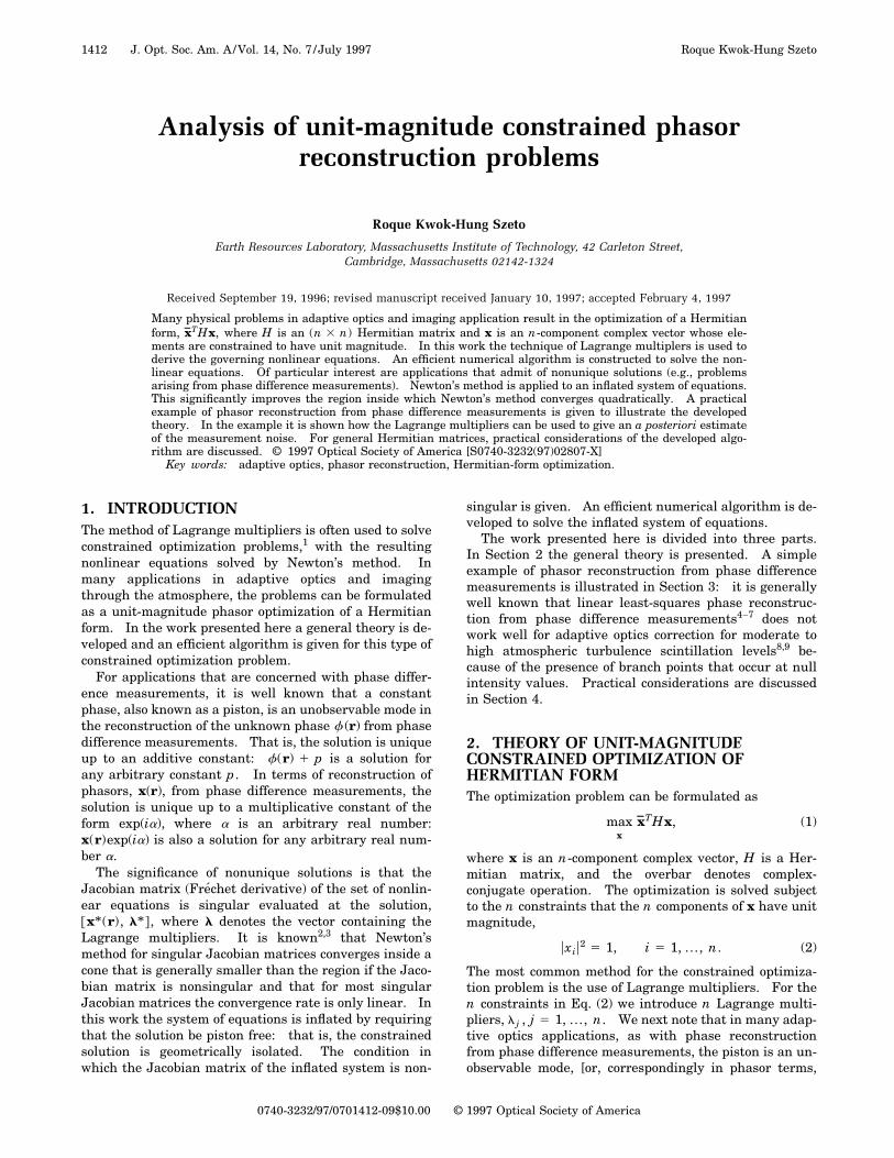
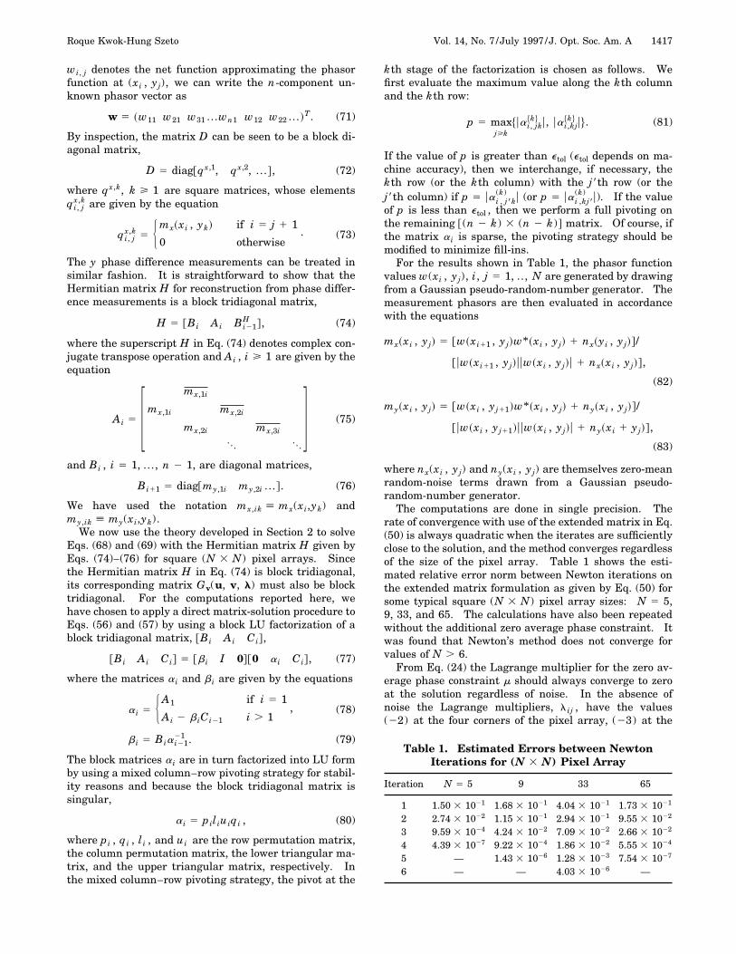
The results shown are for a square (65 3 65) pixel array.Figures 2, 3, 4, and 5 are for the four values of sn :1022,1021, 1, and 10, respectively. The reason that Figs.4 and 5 are comparable is that both measurement noisesare near or at saturation.Of more interest are the effects of measurement noise

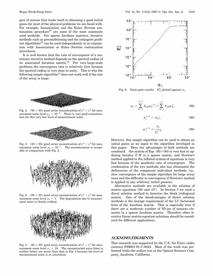
on the mean square reconstructed phasor error. For ourexample, we use the notation Ef

2 to denote the meansquare phase reconstruction error,

Ef2 5

1

N2 (i, j51

N

(arg$wi, j exp@2i~xi2 1 yj

2!#%)2. (91)

Ef2 is plotted as a function of sn in Fig. 6. The curve is

obtained from the average of 60 different realizations foreach of the sn values.

4. PRACTICAL CONSIDERATIONS FORGENERAL HERMITIAN MATRICESThe success of Newton’s method in the solution of systemsof nonlinear equations lies in the ability to obtain a suffi-ciently good initial guess that lies inside the ball of con-vergence. Unfortunately, obtaining a good initial guessis problem dependent. Fortunately, there is a certain as-

Fig. 1. Effects of measurement noise on Lagrange multipliers:mean square of the deviation of Lagrange multipliers from theircorresponding noise-free values plotted as a function of sn forsquare (N 3 N) pixel array, N 5 33 (jagged line), and N 5 65and 129, the curves for the two larger N values are indistinguish-able. The result here can provide an a posteriori estimate of thefidelity of the measurement data.


pect of science that lends itself to obtaining a good initialguess for most of the physical problems we are faced with.For example, linearization and the Euler–Newton con-tinuation procedure10 are some of the most commonlyused methods. For sparse Jacobian matrices, iterativemethods such as preconditioning and the conjugate gradi-ent algorithms12 can be used independently or in conjunc-tion with linearization or Euler–Newton continuationprocedures.It is well known that the rate of convergence of a sta-

tionary iterative method depends on the spectral radius ofits associated iteration matrix.13 For very-large-scaleproblems the convergence rate is relatively slow becausethe spectral radius is very close to unity. This is why thefollowing simple algorithm14 does not work well if the sizeof the array is large:

Fig. 2. (65 3 65) pixel array reconstruction of x2 1 y2 for mea-surement noise level sn 5 1022. There is very good reconstruc-tion for this very low level of measurement noise.

Fig. 3. (65 3 65) pixel array reconstruction of x2 1 y2 for mea-surement noise level sn 5 1021. The reconstruction is accept-able in comparison with Fig. 2.

Fig. 4. (65 3 65) pixel array reconstruction of x2 1 y2 for mea-surement noise level sn 5 1. The degradation due to measure-ment noise is clearly evident.

Fig. 5. (65 3 65) pixel array reconstruction of x2 1 y2 for mea-surement noise level sn 5 10. The reconstructed wave front isneither better nor worse than that in Fig. 4 because the level ofmeasurement noise is at saturation.

uj 5 (k51

j21

hjkwkn11,1(

k5j

n

hjkwkn , (92)

l jn11 5 uuju, (93)

wjn11 5

uj

l jn11 . (94)

However, this simple algorithm can be used to obtain aninitial guess as an input to the algorithm developed inthis paper. Here the advantages of both methods arecombined: the system of Eqs. (92)–(94) is very fast in up-dating iterates if H is a sparse matrix, and Newton’smethod applied to the inflated system of equations is veryfast because of the quadratic rate of convergence. Thecombination of the two methods also has eliminated thedeficiencies of the component individual methods, viz.,slow convergence of the simple algorithm for large arraysizes and the difficulty in convergence if Newton’s methodis applied to any arbitrary initial guesses.Alternative methods are available in the solution of

matrix equations (56) and (57). In Section 3 we used adirect solution method to factorize the block tridiagonalmatrix. One of the disadvantages of direct solutionmethods is the storage requirement of the LU factorizedform of the Jacobian matrix. This is especially true ifthere are a moderate number of fill-ins of nonzero ele-ments in a sparse Jacobian matrix. Therefore other it-erative linear matrix-equation solutions should be consid-ered for different applications.

ACKNOWLEDGMENTSThis research was supported by the U.S. Air Force undercontract F29601-91-C-0023. Most of the work was per-formed while the author was at the Optical Sciences Com-pany, Anaheim, California.

Fig. 6. Noise gain results: Ef2 plotted against sn .


REFERENCES1. P. E. Gill and W. Murray, Numerical Methods for Con-

strained Optimization (Academic, New York, 1974).2. L. Rall, ‘‘Convergence of the Newton process to multiple so-

lutions,’’ Numer. Math. 9, 23–37 (1966).3. G. W. Reddien, ‘‘On Newton’s method for singular prob-

lems,’’ SIAM J. Numer. Anal. 15, 993–996 (1978).4. R. H. Hudgin, ‘‘Wave-front reconstruction for compensated

imaging,’’ J. Opt. Soc. Am. 67, 375–378 (1977).5. J. Hermann, ‘‘Least-Squares wave-front errors of minimum

norm,’’ J. Opt. Soc. Am. 70, 28–35 (1980).6. H. Takajo and T. Takahashi, ‘‘Least-squares phase estima-

tion from the phase difference,’’ J. Opt. Soc. Am. A 5, 416–425 (1988).

7. B. M. Welsh and C. S. Gardner, ‘‘Performance analysis ofadaptive optics systems using laser guide stars and slopesensors,’’ J. Opt. Soc. Am. A 6, 1913–1923 (1989).

8. H. Takajo and T. Takahashi, ‘‘Suppression of the influenceof noise in least-squares phase estimation from the phasedifference,’’ J. Opt. Soc. Am. A 7, 1153–1162 (1990).

9. D. L. Fried and J. L. Vaughn, ‘‘Branch cuts in the phasefunction,’’ Appl. Opt. 31, 2865–2882 (1992).

10. H. B. Keller, ‘‘Bifurcation and nonlinear eigenvalue prob-lems,’’ in Applications of Bifurcation Theory, P. Rabinowitz,ed. (Academic, New York, 1977), pp. 359–384.

11. J. H. Wilkinson, The Algebraic Eigenvalue Problem (OxfordU. Press, Oxford, 1965).

12. O. Axelsson, Iterative Solution Methods (Cambridge U.Press, Cambridge, 1994).

13. D. M. Young, Iterative Solution of Large Linear Systems(Academic, New York, 1971).

14. R. A. Hutchin, Optical Physics Consultants, RedondoBeach, Calif. 90277 (personal communication, 1996).

analysis of unit-magnitude constrained phasor reconstruction problems

Documents