analysis of the vehicle-track-structure...

COMPDYN 2011ECCOMAS Thematic Conference on

Computational Methods in Structural Dynamics and Earthquake Engineering M. Papadrakakis, M. Fragiadakis, V. Plevris (eds.)

Corfu, Greece, 25-28 May 2011

ANALYSIS OF THE VEHICLE-TRACK-STRUCTURE-SOIL DYNAMICINTERACTION OF RAILWAY BRIDGES FOR HST

A. Romero, J. Domınguez, P. Galvın

Escuela Tecnica Superior de Ingenieros. Universidad de Sevilla.Camino de los Descubrimientos, 41092 Sevilla, Spain

[email protected], [email protected], [email protected]

Keywords: High speed train (HST), Soil structure interaction, Railway bridge, Resonant vibra-tion.

Abstract. The dynamic vehicle-track-bridge-soil interaction is studied on high speed lines. Theanalysis is carried out using a general and fully three dimensional multi-body-finite element-boundary element model, formulated in the time domain to predict vibrations due to the trainpassage over the bridge. The vehicle is modelled as a multi-body system, the track and thebridge are modelled using finite elements and the soil is considered as a homogeneous half-space by the boundary element method. Usually, moving force model and moving mass modelare employed to study the dynamic response of bridges. In this work, the multi-body systemallows one to consider the quasi-static and dynamic excitation mechanisms. Soil-structureinteraction is taken into account on the dynamic behaviour on simply-supported short spanbridges. The influence of soil-structure interaction is analysed in both resonant and non-resonant regimes.

1


1 INTRODUCTION

Resonance phenomenon on railway bridges occurs when the loading frequency is close toa multiple of a natural frequency of the structure. In short-span bridges, actual operation ve-locity could be higher than resonance velocities. In that case, high level vibrations reached onresonance regime can result in problems to the security, passenger comfort and track stabil-ity. Therefore, the dynamic behaviour of railway bridges becomes an important design issue.Bridge behaviour is influenced by many factors such as the axle load, successive load passageand track irregularities. These effects are evaluated by dynamic amplification factors on railwaybridge standards, which represent the amplification in the dynamic response in relation with thestatic response for a single moving load [1]. However, the dynamic amplification factors do notaccount for the resonance effects and its use is limited to trains speed below220 km/h. In othercases, it is required further analysis.

References about the dynamic response of railway bridges are quite extensive. Fryba [2] pre-sented a theoretical model of a bridge using the integral transformation method. An estimationof the amplitude of the free vibration was given. Li et al. [3]investigated the influence of thevehicle-bridge interaction on resonant vibrations. They concluded that the maximum responsein resonant regime is reached at the first resonance velocity. Ju et al. [4] suggested a three-dimensional finite element model to study resonant effects on multi-span bridges, concludingthat loading frequencies and natural frequencies of bridges should be as different as possibleto avoid resonance phenomenons. Xia et al. [5] investigatedthe resonance mechanisms andconditions of train-bridge system, analysing the resonantregimens according to their excitationmechanisms.

One of the first steps in the study of railway bridge vibrations is to develop an accuratemodel of the induced force by the train. Different vehicle-bridge interaction models have beenused: moving load model, moving mass model and moving oscillators models. The movingforce model is the simplest vehicle-bridge interaction model. The model can be used if thetrain speed is low enough to neglect its inertia. The model has been widely employed by thescientific comunity [6, 7, 8, 9]. Most sophisticated model isthe moving mass model. Thismodel takes into account the mass of the vehicle, but the model does not consider the effectof the suspension. Finally, comprehensive moving oscillator models have been used by severalauthors [3, 4, 5, 10, 11]. Pesterev et al. [10] examined the asymptotic behaviour of the movingoscillator for large and small values of the suspension. Forinfinite spring stiffness, the movingoscillator model is not equivalent to the moving mass model.Liu et al. [11] studied underwhich conditions dynamic train-bridge interaction must beconsidered for the dynamic analysisof railway bridges. They have concluded that the dynamic vehicle-bridge interaction is moreimportant for large train-bridge mass ratio. Li and Su [3] established that the dynamic vehicle-bridge interaction leads a lower level dynamic response of the bridge than the moving forcemodel.

The number of publications about the influence of soil-structure interaction (SSI) on railwaybridges vibrations is reduced. Takemiya et al. [12, 13] studied the soil-foundation-bridge in-teraction under moving loads using a dynamic substructure method in the frequency domain.Recently,Ulker-Kaustell et. al [14] presented a qualitative analysis of dynamic the soil-structureinteraction on a frame railway-bridge. That work is based onTakemiya’s work.

In this work, a three dimensional numerical model is developed to study vehicle-track-structure-soil interaction (Fig. 1). The numerical model is based on the three dimensionalfinite element and boundary element formulation in the time domain. The articulated train con-

2


figuration is modelled as a multi-body system. Therefore, quasi-static and dynamic excitationmechanisms are considered.

ΩFEM

ΩBEM

Figure 1: Vehicle-track-structure-soil interaction.

The outline of this papers is as follows. First, the numerical model is presented, including abrief summary of finite element and boundary element time domain formulation, and the multi-body model used to represent the vehicle-track-structure-soil interaction. Second, the influenceof soil-structure interaction on the dynamic properties ofthe bridge is analysed. Third, thecontribution of the dynamic excitation mechanisms due to high speed train passage are studied.Finally, induced vibrations on a simply-supported short span bridge are computed for severaltrain speeds. Resonant and non-resonant regimes are studied. The influence of soil-structureinteraction in the vibrations of railway bridge is considered.

2 Soil-structure interaction model

The model is based on the three-dimensional finite element [15] and boundary element [16]time domain formulations.

The boundary element method system of equations can be solved step-by-step to obtain thetime variation of the boundary unknowns; i.e. displacements and tractions. Piecewise constanttime interpolation functions are used for tractions and piecewise linear functions for displace-ments. Nine node rectangular quadratic elements are used for spatial discretization. Explicitexpressions of the fundamental solution of displacements and tractions corresponding to animpulse point load in a three dimensional elastic full-space can be seen in reference [17].

Once the spatial and temporal discretizations are carried out it is obtained the followingequation for each time step:

Hnnun = Gnnpn+n−1∑

m=1

(Gnmpm− Hnmum) exp [−2πα(n−m)∆t]

(1)

where,un is the displacement vector andpn is the traction vector at the end of the time intervaln, andHnn andGnn are the full unsymmetrical boundary element system matrices, in the timeintervaln, α is the soil attenuation coefficient and∆t is the time step. An approach based on theclassical Barkan expression [18] is employed to account forthe material damping in the soil;the right hand side term derived from previous steps is damped by an exponential coefficientαusing a linearly increasing exponent with time.

The equation which results from the finite element method canbe expressed symbolically asfollows if an implicit time integration Newmark method is applied [19]:

Dnnun = fn + fn−1 (2)

3


whereDnn is the dynamic stiffness matrix,un the displacement vector andfn the equivalentforce vector, in the time intervaln.

In this paper, damping matrixC is considered proportional to mass matrixM and stiffnessmatrixK :

C = α0M + α1K (3)

α0 andα1 are obtained fromith andjth modal damping ratios (ζi andζj, respectively). Thenth

modal damping ratio is [20]:

ζn =α0

2ωn+

α1ωn

2(4)

The ith andjth modes should be chosen to obtain the damping ratios for all modes that con-tribute at the response. If both modes have the same damping ratio ζ , it is obtained:

α0 = ζ2ωiωj

ωi + ωj

α1 = ζ2

ωi + ωj

(5)

Coupling boundary element and finite element sub-regions entails satisfying equilibrium andcompatibility conditions at the interface between both regions [21].

3 Vehicle model

The multi-body model used to represent the vehicle-structure-soil dynamic interaction isshown in figure 2.(a). Axles and car bodies are considered rigid parts. Primary and secondarysuspensions are represented by spring and damper elements [22].

(a)

2lc,i

xc,1

ϕc,1 M

c,1 J

c,1

xc,2

ϕc,2 M

c,2 J

c,2

xc,i

ϕc,i M

c,i J

c,i

(b)

xbc,1

xbc,2

xbc,3

xbc,4

xbc,j-1

xbc,j

Figure 2: (a) The multi-body model for an articulated HST. (b) Uncoupled bogies.

The equations of motion for the uncoupled multi-body systemshown in Fig. 2.(b) can bewritten as follows:

M x + Cx + Kx = F (6)

where,M , C andK are the mass, damping and stiffness matrices, respectively. Vehicle responseis described by the displacementxc and rotationϕc of the body, the displacementxb and rotationϕb of the bogies, and the displacement of the wheelsxwr andxwf .

4


x

2lw

k1, c

1

Mb, J

b

k2, c

2

Mw

Mw

xw,r

xw,f

xbc

xb

ϕb

Figure 3: The multi-body model for a bogie.

The mass matrix of each bogie (Eq. 7) is composed of the bogie massMb, the bogie inertiamomentJb and wheel massesMw:

M b = diag (0 Mb Jb Mw Mw) (7)

The stiffness and damping matrices of a bogie can be written as:

K b =

k2 −k2 0 0 0−k2 2k1 + k2 0 −k1 −k10 0 2k1l

2w −k1lw k1lw

0 −k1 −k1lw k1 00 −k1 k1lw 0 k1

(8)

Cb =

c2 −c2 0 0 0−c2 2c1 + c2 0 −c1 −c10 0 2c1l

2w −c1lw c1lw

0 −c1 −c1lw c1 00 −c1 c1lw 0 c1

(9)

where,k1 andc1 are the stiffness and damping of the primary suspension,k2 andc2 are thestiffness and damping of the secondary suspension, and2lw is the distance between axles of abogie.

The equation of motion of the whole train can be obtained fromdisplacement relationshipsbetween car bodies and bogies. The relationshisp to obtain the equation of motion of the fronttraction car [22] are:

xbc,1 = xc,1 − ϕc,1lc

xbc,2 = xc,1 + ϕc,1lc(10)

where,xc,1 andϕc,1 represent vertical displacement and rotation of the car body, respectively,and2lc the bogie distance in a vehicle. Similar expression can be drawn for the first passengercar (Fig. 2). The vertical displacementxbc,n for themth vehicle can be written as follows:

xbc,n = 2

m∑

i=3

(

(−1)n+ixc,i

)

+ (−1)n (xc,2 + lc,2ϕc,2) (11)

The relationships for the whole train can be expressed as:

xbc = Lx c (12)

5


(a)

0.70

1.39 1.39 1.39 1.39

0.25

0.75

5.84

0.3 0.3 0.3 0.3

1.46

1.30

0.72

UIC-60

Concrete sleeper

0.3

Ballast layer

Rail-pad

(b)

1.20

1.20

1.20

2.40

7.30

6.00

Figure 4: (a) Deck cross-section. (b) Abutment geometry.

Introducing Eq. (12) into Eq. (6) lead to:

Mx + Cx + Kx = F (13)

where,M , C andK are the mass, damping and stiffness matrices of the articulated HST (Fig.2.(a)). The mass matrix is obtained by assembling car body mass matrix:

M c = diag (Mc Jc) (14)

whereMc is the mass of the car body andJc the inertia moment of the car body. The degree offreedom of rotation of the vehicle allows us to consider the pitch car inertia moment.

Finally, the equation of motion of the vehicle is introducedin the soil-structure interactionequation imposing equilibrium and compatibility conditions at each wheel-rail contact point.A Hertzian contact spring is considered between wheels and rails [22, 23]. As vehicle movesalong the track according to its speed, contact points between wheels and rails change as timegoes on. A moving node is created at each wheel-rail contact point in the rail to couple vehiclesand track. So the track mesh including rail changes at each time step. Then, mass, dampingand stiffness matrices vary at each time step and the obtained finite element system of equationsbecomes non-linear. Nevertheless, the time domain formulation allows one to solve the non-linear system of equations using, for example, the methodology presented in reference [24].

4 Dynamic behaviour of simply-supported short span bridge

In this section, the dynamic behaviour of a simply-supported short span bridge under HSTpassage is studied. First, the modal properties are obtained account for soil-structure interac-tion. Second, the quasi-static and the dynamic load contribution are studied. Finally, the dy-namic response of the bridge due to HST passage is analysed taken into account soil-structureinteraction.

4.1 Soil-structure dynamic interaction

In this paper a railway bridge with a single suported slab bayof 12m is studied. The deck(Fig. 4.(a)) is composed of a0.25m thickness concrete slab. The slab resting over five pre-stressed concrete beams with a0.75 × 0.3m rectangular cross-section. A distance1.39m be-tween beams is considered. The concrete has a densityρ = 2500 kg/m3, a Poisson ratioν = 0.2,and a Young’s modulusE = 31× 109 N/m2.

6


The deck leans over two concrete abutments (Fig. 4.(b)) withdensityρ = 2500 kg/m3, aPoisson ratioν = 0.3, and a Young’s modulusE = 20×109 N/m2. Beams resting on laminatedrubber bearings. The bearings have a thickness of20mm and the stiffness and damping valuesarekb = 560× 106 N/m andcrp = 50.4× 103 Ns/m.

A single ballast track is located over the deck. The track is composed of two UIC60 railswith a bending stiffnessEI = 6.45 × 106 Nm2 and a mass per unit lengthm = 60.3 kg/m foreach rail. The rail-pads have a10mm thickness and their stiffness and damping values arekrp =150 × 106 N/m andcrp = 13.5 × 103 Ns/m, respectively. The prestressed concrete monoblocksleepers have a lengthl = 2.50m, a widthw = 0.235m, a heighth = 0.205m (under therail) and a massm = 300 kg. A distanced = 0.6m between the sleepers is considered. Theballast has a densityρ = 1800 kg/m3, a Poisson ratioν = 0.2, and a Young’s modulus equal toE = 209× 106 N/m2. The width of the ballast equals2.92m and the heighth = 0.7m.

The structure is assumed to be located at the surface of a homogeneous half-space that rep-resents a stiff soil, with a S-wave velocityCs = 400.0m/s, a P-wave velocityCp = 799.4m/s,and a Rayleigh wave velocityCR = 372.6m/s.

ΩFEM

ΩBEM

Figure 5: Soil-structure discretization.

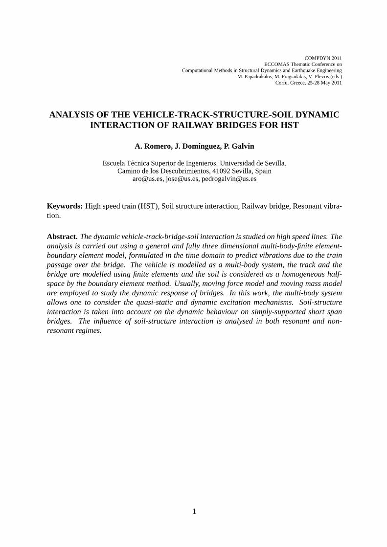
Fig. 6 shows the first four mode shapes, corresponding with the first bending (symmetric),the first torsional, the first bending of cross-section (symmetric) and the first antisymmetricbending deck mode shapes, respectively.

Fig. 7 shows the vertical displacement at the center of the mid-span deck due to an impulsiveloadP (t) = −1N (H(t)−H(t−0.045 s)) acting in both rails. The response is governed by thefirst bending (symmetric) deck mode. The same structural damping is considered for all modesthat contribute significantly to the response of the structureζ = 2%. Damping matrix (Eq. 2) isobtained consideringωi = ω1 andωj = ω4, beingα0 = 2.3 andα1 = 1.24×10−4. Fig. 7 showsthat the resonant frequency moves tof1 = 11.06Hz and an amplification in the response whenSSI is considered. This effect is due to the additional levelof flexibility between the abutmentsand the soil. The damping can be obtained from the free vibration response. Its value increasesto ζ = 3.9% when SSI is considered.

4.2 Quasi-static and dynamic excitation mechanisms

Induced vibrations due to HST passage are generated by several excitation mechanisms: thequasi-static contribution, the parametric excitation dueto the discrete support of the rails and thedynamic contribution due to wheel and rail unevenness. In this section, the different excitationmechanisms are studied.

7


(a) f1 = 11.96Hz (b) f2 = 21.90Hz

(c) f3 = 29.99Hz (d) f4 = 47.82Hz

Figure 6: First four modes of vibrations of the structure.

0 50 100 1500

1

2

3x 10

−9

Frequency [Hz]

Rec

epta

nce

[m/N

/Hz]

Figure 7: Track-structure-soil and track-structure receptance

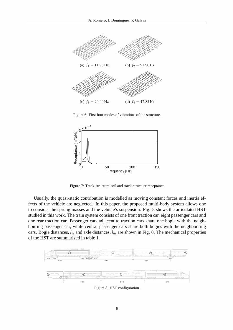
Usually, the quasi-static contribution is modelled as moving constant forces and inertia ef-fects of the vehicle are neglected. In this paper, the proposed multi-body system allows oneto consider the sprung masses and the vehicle’s suspension.Fig. 8 shows the articulated HSTstudied in this work. The train system consists of one front traction car, eight passenger cars andone rear traction car. Passenger cars adjacent to traction cars share one bogie with the neigh-bouring passenger car, while central passenger cars share both bogies with the neighbouringcars. Bogie distances,lb, and axle distances,la, are shown in Fig. 8. The mechanical propertiesof the HST are summarized in table 1.

7 108 9

18700 21845 22150

187002184522150

1 2 3 4

30003520 3000 1630 1640 3000 3000

Figure 8: HST configuration.

8


Description Name Unit Traction cars Passenger cars

Mass of car-body Mc kg 55790 24000

Mass of bogie Mb kg 2380 3040

Mass of wheel-axle Mw kg 2048 2003

Car-body inertia moment Jc kg m2 1.15× 103 1.48× 103

Bogie inertia moment Jb kg m2 1.48× 106 2.68× 103

Primary suspension stiffness k1 N/m 2.45× 106 1.4× 106

Secondary suspension stiffnessak2 N/m 2.45× 106 0.82× 106

Primary suspension damping c1 Ns/m 20× 103 10× 103

Secondary suspension damping c2 Ns/m 40× 103 48× 103

Table 1: Mechanical properties of HST

The transmitted load by an axle can be computed as the elasticinteraction forceFH at wheel-rail contact point as follows:

FH = −2kH(uc − uw) (15)

where,uc is the rail displacement at contact point,uw represents the wheel displacement andkH = 1.4 × 109 N/m is a Hertzian contact spring between wheels and rail [23]. Fig. 9 showsthe one-third octave band spectra of the transmitted load for train speedv = 80m/s andV1,2 =110.14m/s. V1,2 is resonant resonant speed of the bridge (see section 4.3). The computedresults are compared with those obtained using a moving force model. Both models lead tothe same results at the bogie passing frequency,fb = v/lb, and the axle passing frequency,fa = v/la. However, the computed transmitted forces present differences at higher frequenciesdue to inertia effects are neglected in the moving force model.

(a)1 2 4 8 16 31.5 63 125

160

180

200

220

One−third octave centre frequency [Hz]

For

ce[d

B, r

ef 1

0−6 N

]

(b)1 2 4 8 16 31.5 63 125

160

180

200

220


For

ce[d

B, r

ef 1

0−6 N

]

Figure 9: Excitation force on the track computed with a moving force model (grey line) and the multi-body system(black line) for a HST travelling at (a)v = 80m/s and (b)V1,2 = 110.14m/s

9


1 2 4 8 16 31.5 63 12550

60

70

80

90

One−third octave centre frequency[Hz]

Dis

plac

emen

t[d

B, r

ef 1

0−6 m

]

Figure 10: One-third octave band spectra of the vertical displacement at the wheel (red line), bogie (blue line) andthe car body (green line) due to the track unevenness (black line) for a HST travelling atv = 80m/s.

The dynamic contribution account for track and wheel irregularities. The displacement vec-tor uc is equal to the sum of rail displacementur and rail unevennessuw/r perceived by an axle[25, 26]:

uc = ur + uw/r (16)

In this paper, random track unevennessuw/r(x) is modelled as a stationary Gaussian randomprocess characterized by its one-sided PSD functionSuw/r

(ky). The spectral representationtheorem is used to generate samples of track unevennessuw/r(x) as a superposition of harmonicfunctions with random phase angles [25, 26]:

uw/r(x) =n

∑

m=1

√

2Suw/r(kym)∆ky cos(kymy − θm) (17)

wherekym = m∆ky is the wavenumber sampling used only to compute the artificial profile,∆ky the wavenumber step andθm are independent random phase angles uniformly distributedin the interval[0, 2π]. The artificial track profile is generated from PSD function according toISO 8608 [27]:

Suw/r(ky) = Suw/r

(ky0)

(

kyky0

)

−w

(18)

An artificial profile is obtained from the PSD function withky0 = 1 rad/m andSuw/r(ky0) =

2π × 10−8m3. w = 3.5 is commonly assumed for wheel-rail unevenness in current high speedlines.

Fig. 10 shows the one-third octave band spectra of the vertical displacement at the wheel, bo-gie and body car due to the unevenness profile shown in the samefigure. Primary and secondarysuspensions system isolate body car and bogie at frequencies higher than1.2Hz y 5.5Hz, re-spectively.

Figs. 11(a),(b) show the one-third octave band spectra of the vertical acceleration at the cen-ter of the mid-span deck for a train passage atv = 80m/s andV1,2 = 110.14m/s, respectively.The quasi-static contribution are represented in these figures. The deck response is governed bythe quasi-static contribution.

4.3 Induced vibrations due to HST

In this section, SSI effect on induced vibrations due to HST passage is studied. Resonant andnon resonant regimes are analysed. The geometry and the mechanical properties of the bridgehave been described in previous sections.

10


(a)1 2 4 8 16 31.5 63 125

60

80

100

120

140


Acc

eler

atio

n[d

B, r

ef 1

0−6 m

/s2 /H

z]

(b)1 2 4 8 16 31.5 63 125

60

80

100

120

140


Acc

eler

atio

n[d

B, r

ef 1

0−6 m

/s2 /H

z]

Figure 11: The computed total response (black line) and the computed quasi-static (grey line) one-third octaveband spectra of the vertical acceleration at the center of the mid-span deck for a HST travelling at (a)v = 80m/sy (b) V1,2 = 110m/s.

40 60 80 100 1200

10

20

30

Velocity [m/s]

Acc

eler

atio

n [m

/s 2 ]

V1,2=

110.14

m/s

V1,5=

44.06

m/s

V1,7=

31.47

m/s

V1,2=

103.41

m/s

amax = 3.5m/s2

Figure 12: Maximum vertical acceleration at the mid-span center deck computed from SSI model (black line) andnon-SSI model (grey line).

The resonant condition of a bridge excited by a row of moving forces can be expressed asfollows [2, 5]:

Vn,i =fnd

i(n = 1, 2, ..., i = 1, 2, ...) (19)

where,Vn,i is the train speed,fn is thenth resonant frequency of the bridge andd is a charac-teristic distance of the moving loads.

Fig. 12 shows the maximum vertical acceleration at the center of mid-span deck in relationto the train speed passage. There is an increase of deck acceleration when the speed increases.Maximum levels are reached at resonant velocities of the first bending (symmetric) mode shape,considering the distance between bogiesd = 18.7m. Figure 12 shows the resonant velocitiesV1,2 = 110.14m/s,V1,5 = 44.06m/s andV1,7 = 31.47m/s. The Spanish Standard [1] sets a limitstate of vertical accelerations atamax = 3.5m/s2, plotted in Fig. 12. The maximum accelerationat the center of the mid-span deck is below this limit in the range of operating speeds on currenthigh speed lines. The response of the structure varies substantially when SSI is considered.Resonant velocities decrease due to variation of the dynamic behaviour of the structure. Themaximum response occurs atV1.2 = 103.41m/s. Moreover, it is observed that the maximumlevel of acceleration achieved in resonant regime is significantly lower when the soil-structureinteraction is considered. The structural damping varies from ζ = 2% to ζ = 3.9%.

Fig. 13 shows the time histories and frequency content of thevertical acceleration at thecenter of mid-span deck for three train speed passage:v = 80m/s, V1,2 = 103.41m/s andV1,2 = 110.14m/s. In the first case, the response obtained with both modelscorresponds witha non-resonant regime. The time history shows similar levels in both cases and the differences

11


are not significant. The response is governed by the bogie passing frequency, for the first bend-ing (symmetric) mode and the first bending mode of the cross-section. The SSI produces anamplification of the response at the bogie passing frequency. In addition, the frequency re-sponse associated with the natural frequencies of the structure decreases. In resonant regime,the response of the structure shows a gradually increase of the vibrations with the successivebogie passage at the resonant velocitiesV1,2 andV1,2 (Fig. 13.(c),(e), respectively). The pre-dominant frequency in the response are asociated with the first bending mode (Fig. 13.(d),(f)).The model without SSI does not estimate accurately the bridge response as can be seen in Fig.13.(c),(d). Since the amplitude of the resonant vibration depend inversely on damping [2], themodel without soil overestimates the response, as can be seen in Figs. 13.(e),(f).

(a)0 0.5 1 1.5 2 2.5

−5

0

5

Time [s]

Acc

eler

atio

n [m

/s2 ]

(b)0 10 20 30 40 50 60

0

0.5

1

Frequency [Hz]

Acc

eler

atio

n [m

/s2 /H

z]

(c)0 0.5 1 1.5 2

−10

−5

0

5

10

Time [s]

Acc

eler

atio

n [m

/s2 ]

(d)0 10 20 30 40 50 60

0

1

2

3

4

Frequency [Hz]

Acc

eler

atio

n [m

/s2 /H

z]

(e)0 0.5 1 1.5 2

−20

−10

0

10

20

Time [s]

Acc

eler

atio

n [m

/s2 ]

(f)0 10 20 30 40 50 60

0

5

10

Frequency [Hz]

Acc

eler

atio

n [m

/s2 /H

z]

Figure 13: (a,c,e) Time histories and (b,d,f) frequency contents of the vertical acceleration at the mid-span centerdeck for a HST travelling at (a,b)v = 80m/s, (c,d)V1,2 = 103.41m/s y (e,f)V1,2 = 110.14m/s, computed fromthe SSI model (black line) and the non-SSI model (grey line).

5 Conclusions

In this paper, a numerical model to predict vibrations on railway bridges has been presented.The numerical model is based on the three dimensional finite element and boundary element for-mulations in time domain. The articulated HST is modelled asa multi-body system. Therefore,the different excitation mechanisms can be considered accurately. The following conclusionscan be drawn from the obtained results:

1. Transmitted force has a high frequency content that the moving force model does not

12


reproduce accurately due to vehicle’s inertia effects are neglected.

2. Structure soil interaction produces a reduction in the natural frequencies and an increaseof structural damping due to the additional flexibility level between the abutment and thesoil.

3. Therefore, the resonant behaviour occurs at speeds lowerthan those predicted by themodel without soil.

4. The amplitude of the resonant response regime depends on the structural damping ratio.So, it is necessary to take into account the influence of the SSI to estimate correctly theresponse.

Acknowledgments

This research is financed by the Ministerio de Ciencia e Innovacion of Spain under the re-search project BIA2010-14843. The financial support is gratefully acknowledge. The supportgive by the Andalusian Scientific Computing Centre (CICA) isgratefull.

REFERENCES

[1] Ministerio de Fomento,Instruccion sobre las acciones a considerar en el proyecto depuentes de ferrocarril IAPF07, Ministerio de Fomento 2007

[2] L. Fryba, A rough assessment of railway bridges for highspeed trains,EngineeringStructures23 (2001) 548-556.

[3] J. Li, M. Su, The resonant vibration for a simply supported girder bridge under high-speedtrains,Journal of Sound and Vibration224 (1999) 897-915

[4] S.H. Ju, H.T. Lin, Resonance characteristics of high-speed trains passing simply sup-ported bridges,Journal of Sound and Vibration267 (2003) 1127-1141

[5] H. Xia, N. Zhang, W.W. Guo, Analysis of resonance mechanism and conditions of train-bridge system,Journal of Sound and Vibration297 (2006) 812-822.

[6] P. Museros, E. Alarcon, E, Influence of the second bending mode on the response ofhigh-speed bridges at resonance,Journal of Structural Engineering131 (2005) 405-415.

[7] P. Museros, M.D. Martinez-Rodrigo, Vibration control of simply supported beams undermoving loads using fluid viscous dampers,Journal of Sound and Vibration300 (2007)292-315.

[8] M.D. Martınez-Rodrigo, J. Lavado, P. Museros, Transverse vibrations in existing rail-way bridges under resonant conditions: Single-track versus double-track configurations ,Engineering Structures32 (2010) 1861-1875.

[9] M.D. Martınez-Rodrigo, P. Museros, Optimal design of passive viscous dampers for con-trolling the resonant response of orthotropic plates underhigh-speed moving loads,Jour-nal of Sound and Vibration(2010), doi:10.1016/j.jsv.2010.10.017

13


[10] A.V. Pesterev, L.A. Bergman, C.A. Tan, T.-C. Tsao, B. Yang, On the asymptotics of thesolution of the moving oscillator problem,Journal of Sound and Vibration260 (2003)519-536.

[11] K. Liu, G. De Roeck, G. Lombaert, The effect of dynamic train-bridge interaction onthe bridge response during a train passage,Journal of Sound and Vibration325 (2009)240-251.

[12] H. Takemiya, X.C. Bia, Shinkansen high-speed train induced ground vibratios in view ofvıaduct-ground interaction,Soil Dynamics and Earthquake Engineering27 (2007) 506-520.

[13] H. Takemiya, Analyses of wave field from high-speed train on vıaduct at shallow/deepsoft grounds,Journal of Sound and Vibration310 (2008) 631-649.

[14] M. Ulker-Kaustell, R. Karoumi, C. Pacoste, Simplified analysis of the dynamic soil-structure interaction of a portal frame railway bridge,Engineering Structures32 (2010)3692-3698.

[15] O.C. Zienkiewicz,The Finite Element Method, McGraw-Hill Company, London, 1977.

[16] J. Domınguez,Boundary elements in dynamics, Computational Mechanics Publicationsand Elsevier Applied Science, Southampton, 1993.

[17] P. Galvın, J. Domınguez, Analysis of ground motion due to moving surface loads inducedby high-speed trains,Engineering analysis with boundary elements30 (2007) 931–941.

[18] D.D. Barkan,Dynamics of Bases and Foundations, McGraw-Hill, New York, 1962.

[19] N.M. Newmark, A method of computation for structural dynamics,ASCE Journal of theEngineering Mechanics Division85 (1959) 67–94.

[20] R.W Clough, J. PenzienDynamic of Structures, McGraw-Hill, New York, 1975.

[21] P. Galvın, A. Romero, J. Domınguez, Fully three-dimensional analysis of high-speedtrain-track-soil-structure dynamic interaction ,Journal of Sound and Vibration329 (2010)5147–5163.

[22] X. Sheng, C.J.C. Jones, D.J. Thompson, A theoretical model for ground vibration fromtrains generated by vertical track irregularities,Journal of Sound and Vibration272 (2004)937–965.

[23] C. Esveld,Modern Railway Track, MRT Productions,Zaltbommel, 2001.

[24] S.Y. Chang, Nonlinear error propagation analysis for explicit pseudodynamics algorithm,Journal of engineering mechanics ASCE123 (2003) 841–850.

[25] G. Lombaert, G. Degrande, J. Kogut, S. Francois, The experimental validation of a nu-merical model for the prediction of railway induced vibrations, Journal of Sound andVibration297 (2006) 512–535.

[26] G. Lombaert, G. Degrande, Ground-borne vibration due to static and dynamic axle loadsof InterCity and high-speed trains,Journal of Sound and Vibration319 (2009) 1036–1066.

14


[27] International Organization for Standardization ISO 8608:1995,Mechanical vibration roadsurface profiles-reporting of measured data, 1995.

15

analysis of the vehicle-track-structure...

Documents