analysis of the effect of oil price shock on industry
TRANSCRIPT

1 | P a g e
Analysis of the Effect of Oil Price Shock on Industry
Stock Returns in Nigeria
by
Magnus O. Abeng1
Research Department, Central Bank of Nigeria
Abstract
This study focus on the impact of oil price fluctuation on the sector level activities of the stock
market in Nigeria. Five industry sectors were examined based on availability of data while
included macroeconomic factors were selected guided by economic theory and existing
literature. Study results suggest that changes in oil prices significantly affect stock returns of all
the sectors, except food beverages and tobacco. Consistent with the findings of McSweeney
and Worthington (2007) and Agusman and Deriantino (2008) for the Australian and Indonesian
stock markets, respectively, the parameter estimates of market returns for the banking,
insurance, food beverages and tobacco, oil and gas and industrial sectors significantly
exceeded unity, suggesting a high risk exposure of these sectors vis-à-vis market returns. The
food beverages and tobacco and oil and gas sectors exhibit significantly negative sensitivity to
exchange rate risk, indicating the debilitating effect of the depreciation of the domestic
currency on the returns of these sectors. The implications are enormous. First, the negative
response of all sectors to exchange rate movement calls for prudent management of reserves
plus informed and timely intervention in the market by the monetary authority to keep the rate
stable. Secondly, the insensitivity of the food beverages and tobacco to oil price movement is
an indication of the inefficiency instituted by the subsidy on petroleum products that insulate
domestic consumption from market fundamentals. Subsidies distort the efficient allocation of
resources by the market and in the case of Nigeria abet and aid corruption.
Key Words: Stock market shocks, oil price fluctuation, industry sector returns
JEL Classification: F42, E52
1 Magnus Abeng is a staff of the Research Department of the Central Bank of Nigeria and a PhD student at
the University of Surrey, United Kingdom. The views expressed herein are the author’s and not those of the
institutions he is affiliated with. E-mail: [email protected] or [email protected]

2 | P a g e
1. Introduction
The role of oil resource and the implications for its changing prices on the global
economy has been extensively examined in the literature (Hamilton, 1983; Mork, 1989;
Jones and Kaul, 1996; Balaz and Londarev, 2006; Kilian, 2007; Rault and Arouri, 2009;
Jones et al, 2004; and Chittedi, 2012), among others. As the world’s leading fuel, oil
resource is unarguably an essential factor input in the production process, accounting
for 32.9 per cent of global energy consumption, and over 61.0 per cent of global trade
in 2013 (BP, 2014). This significant role underscores the extensive literature on the
implications oil price changes on key macroeconomic indicators as inflation rate,
exchange rate, interest rate, stock prices, international debt and output growth2.
Though these studies differ markedly in their findings, they nevertheless, affirm the
degree of risk the global economy is exposed to in the face oil price fluctuations. Some
of the noted effects of positive changes in oil price include exacerbated inflationary
pressure; reduced real disposable income; dampened aggregate demand;
decelerated investment; worsened unemployment rate; and eventually slowed down
economic growth. These claims were clearly attested to by the macroeconomic
distortions that accompanied the global oil crisis of the 1970s, the international Persian
Gulf crisis of 1991 and, to a large extent, the recent 2007/2008 global financial and
economic crisis. Though the degree of transmission of oil price shocks to the economy
depends on whether the economy is oil-exporting or oil-importing, such consequences,
in many climes, extend beyond the economic to the social spheres where oil price
shocks are felt much more by the poor than the developed economies. (McSweeney
and Worthtington, 2007 and Rifkin, 2002),
The Nigerian economy is overly dependent on crude oil exports, which contribute
about 98 per cent of export earnings, 83 per cent of Federal government revenue and
a key contributor to GDP (CBN, 2001). The proceeds from crude oil exports in 2002
accounted for over 70 per cent of government revenue, 90 per cent of foreign
exchange earnings, and 26 per cent of GDP. By 2006, the proportions of oil exports to
government revenue, GDP and foreign exchange earnings increased to 87.2, 37.6 and
90.2 per cent, respectively, while in 2010 earnings from oil alone contributed
approximately 94.0 per cent of total foreign exchange (CBN 2010b).
These statistics underscores the vulnerability of the economy to the vagaries of
international crude oil price. Theoretically, an increase in oil price should indicate
2 Hamilton (1983); Chen et al (1986); Gisser and Goodwin (1986); Mork (1989); Huang et al (1996); Jones and Kaul
(1996); Sadorsky (1999); Koranchelin (2005); Balaz and Londarev (2006); Barsher and Sadorsky (2006), Kilian
(2007); and Kilian and Park (2008); Rault and Arouri, 2009; Jones et al, (2004); and Chittedi, (2012).

3 | P a g e
revenue windfall for oil-exporting countries as it is expected to shore up foreign
exchange earnings and build reserve in the short-run. However, for net-importers of
refined petroleum products such as Nigeria with domestic regulation of prices
(subsidies), oil price increase may not translate to the expected economic benefit, but
might rather cascade into severe fiscal hiccups, restraining government’s ability to
finance the huge import bills as well as meet other international obligations. The
aftermaths may be detrimental to economic growth arising from increased domestic
production cost and decline in aggregate demand. Consequently, the impact of oil
price fluctuation on exchange rate, monetary policy, government expenditure, and
stock market in Nigeria has severally been investigated. Evidence from a survey of
these literature3 were mixed, ostensibly due to the different methodologies and data
frequencies employed (Adebiyi et al, 2009 and Aliyu, 2009). Some other studies
undermined the significant contribution of the stock market in the conduct of monetary
policy by excluding stock market indicators in their models (Umar and Kilishi, 2010;
Iwayemi and Fowowe, 2010; and Olomola and Adejumo, 2006). Invariably, conclusions
from these studies are very likely to be bias, misleading and not devoid of meaningful
contributions to monetary policy formulation due to mis-specification and/or other
errors.
In the spirit of globalization and economic integration, research interest has generally
shifted to examining the impact of oil price on the stock market returns plausibly due to
the growing importance of stock market as a channel of monetary policy, in addition to
the growing role of the market as the source of financing long-term development
projects. However, extant literature indicate that most of these studies adopted the
aggregate analytical approaches which mask the dynamics inherent in the market as
the effect of oil price change is apportioned equally across sectors without taking
cognizance of the heterogenous and industry specific features of the sectors. However,
there is an emerging body of literature that is focused at addressing this limitation in the
literature. These studies adopt industry level approach to the analyses of the impact of
oil price shocks on stock market returns making study results veritable input to portfolio
investors’ decision making process and the conduct of monetary policy. It has also
facilitated monetary authority’s better understanding of the role of the stock market as
a channel of monetary policy transmission mechanism and identifies the underlying
factors that drive individual industries’ sensitivity or risk exposure to oil prices changes. In
economies where these studies had been conducted, economic agents had achieved
better economic management and effective decision making processes. To the best of
3 This include Ayadi, et al (2000); Ayadi (2005); Olomola and Adejumo (2006); Sill (2007); Aliyu (2009); Omisakin et al
(2009); Adebiyi et al (2009); and Iwayemi and Fowowe (2010).

4 | P a g e
our knowledge, no study has so far attempted to use this approach in the context of
Nigeria.
Thus, this study attempts to fill this gap by i) including stock market variables in the
model to capture the interaction and dynamics between oil price and stock market
returns, ii) employing high frequency data, which according to Basher and Sadorsky
(2006) contain richer information than lower frequency data, and iii) following the stock
market classification, adopting the microeconomic approach, with a view to analyzing
the relative impact of oil price change on the activities of these individual stock returns.
The objective here is two-pronged: first, to investigate the degree of vulnerability or
otherwise of industry level stock returns to oil price shock, and secondly to examine the
persistence of oil price shocks in Nigerian stock market. To achieve this, the study
followed an approach prevalent in the literature (Faff and Brailsford, 1999; Sadorsky,
2001; Sadorsky and Henriques, 2001; Driesprong, et al, 2004; McSweeney and
Worthington, 2007; and Broadstock, et al, 2012) to first estimate an extended standard
multifactor model to determine the impact of oil price shock on industry stock returns.
The preference for this estimation technique is informed by its ability to reveal the
degree of exposure or level of vulnerability of the various activity sectors in the model
sample to fluctuations in oil price. Consequently, three models would be estimated to
measure the sensitivity of individual sector returns to changes in oil price.
The study is structured into five sections. Following this introduction is Section two, which
reviews both the theoretical, methodological and empirical literature. Specifically,
empirical studies were reviewed with a view to establishing the theoretical platform for
the study. Section three highlights the evolution and developments in the Nigerian stock
capital market as well as the movements in oil price during the sample period. Section
four focused on the methodology, which incorporates the data, model specification
and technique of analysis. The summary and conclusion and study limitations and areas
for further study are the focus of Section five.

5 | P a g e
2. Review of Empirical Literature
Authors Focus Methodology Findings
Huang, et al, (1996) examines the co-movements between
daily returns of oil future with stock
returns during the 1980s
multivariate vector
autoregression (VAR)
approach
could not find any correlation between
oil future and stock returns
Hunt and Witt (1995) Examines the influence of energy
price, income and temperature on
energy consumption in UK
Johansen Maximum
likelihood procedure
L-R relationship between energy
demand, income and price but S-R
effect of temperature
McSweeney and
Worthington (2007)
examine the impact of oil prices on
the stock returns of nine industries in
the Australian market
multifactor model strong positive covariance between oil
price changes and the energy industry
even though the banking, materials,
retailing and transportation industries,
exhibited negative relationship
Yurtsever and Zahor
(2007)
the reaction of stock returns to oil price
shocks as well as the symmetry of this
shock on firms and industries in the
Netherlands
standard market model,
augmented by the oil
price factor
result shows a significant negative effect
of oil price shock on the stocks of some
industries and individual firms (including
banks and chemical industries)
Bredin and Elder
(2011)
the exposure of 18 industry level stock
returns to oil price changes in the US
the linear factor model
(Arbitrage Pricing Theory
(APT))
a weak direct exposure of majority of the
industry returns to oil price changes was
also demonstrated

6 | P a g e
Authors Focus Methodology Findings
Hunt and Witt
(1995)
Examines the influence of energy
price, income and temperature on
energy consumption in UK
Johansen Maximum
likelihood procedure
L-R relationship between energy
demand, income and price but S-R
effect of temperature
McSweeney and
Worthington (2007)
examine the impact of oil prices on
the stock returns of nine industries in
the Australian market
multifactor model strong positive covariance between oil
price changes and the energy industry
even though the banking, materials,
retailing and transportation industries,
exhibited negative relationship
Yurtsever and
Zahor (2007)
the reaction of stock returns to oil
price shocks as well as the
symmetry of this shock on firms and
industries in the Netherlands
standard market
model, augmented
by the oil price
factor
result shows a significant negative effect
of oil price shock on the stocks of some
industries and individual firms (including
banks and chemical industries)
Eryigit (2009) Examined oil price change and the
sectoral indices of the Istanbul
Stock Exchange (ISE)
ordinary least square
technique
changes in oil price having statistically
significant effects on industry level
returns of all the sectors except
transport, banks
Fan and Jahan-
Parvar (2011)
the predictability of the spot and
futures oil price fluctuations on
forty-nine industry-level returns in
the US stock market.
Jump-GARCH model only very few industry returns (20 per
cent) are predictively sensitive to oil spot
price innovations,

7 | P a g e
Overall, it could be deduced from the ample empirical evidence that the impact of oil
price change on industry stock returns, though mixed, cannot be disregarded.
Inference from the review of industry stock returns revealed that the level of exposure of
risk varies across industries. While many studies found no statistically significant
correlation between oil price and industry stock returns, others recorded
contemporaneous reaction of stock prices to oil price shock. This is of particular interest
to investors and policymakers especially as the sensitivity across industries informs them
about the transmission mechanism of oil price shock to the economy, the source of
such shocks and the likely direction of shift in demand for goods and services. This calls
for further research, especially as it was noted that several of these studies focused on
advanced economies, ostensibly due the sophistication of their stock market and
efficient data collection mechanism compared with those of less developed
economies. The dearth of literature for sub Saharan Africa cum Nigeria was noted while
the methodology and data frequency used were fraught with limitations. These
observed gaps served as the motivating factors, which this study intends to contribute
to and fill.
3. Data and Variables Definition
3.1 Data
Data used in this study are sourced from various relevant institutions and agencies. The
all-share-index (ASI) – an indicator of returns in the equity market - and inflation rate,
derived from consumer price index (CPI) – were sourced from the Nigeria Stock
Exchange (NSE) and the National Bureau of Statistics (NBS) databases, respectively.
While real interest rate (RIR) and average nominal exchange rate (EXR) are sourced
from the Central Bank of Nigeria Statistical Bulletin, oil price (OPR) is obtained from the
Energy Information Administration (EIA) of the U.S. Department of Energy. A dummy
(dum07) is incorporated to capture the systemic influence of the global financial crisis
on equity market returns in Nigeria.
The selection of variables was guided by economic theory and related empirical
literature centered on the assumptions of small open economy. Consequently, interest
rate is included in the model to capture the effect of monetary policy, inflation rate
measures real economic activity, the exchange rate reflects the transmission channel in
an open economy, while the role of the dummy variable to capture the effect of the
global financial crisis. The choice of variables is hinged on the fact that stock prices are
known to be susceptible to oil price change and also to changes in other
macroeconomic or market fundamentals.
The study employs monthly data spanning from 1997M1 to 2014M5. The use of monthly
series is justified by previous literature on the subject (Sadorsky, 2001; Sadorsky and

8 | P a g e
Henrques, 2001; and Elsharif et al 2005). Monthly series also streamlines the various data
frequencies, since most macroeconomic variables are not available at higher
frequency as stock returns. Except for real interest rate that is already expressed in
percentages, all other variables are expressed in log form to allow for a unit change in
them to be interpreted as percentage changes. The series are also annualized (year-
on-year basis) to strip them of seasonal effects as well as accommodate investors’
adaptive approach to decision making process.
3.1.2 Variables Definition
The reclassification of industry sectors by the Nigeria Stock Exchange (NSE) in 2009, with
a view to aligning the market with the global industry classification standards (GICS),
led to the streamlining of the number of industry sectors from thirty-three to twelve. Of
the twelve broad representative industry sectors, the study used only five sectors’
indices namely banking, insurance, food beverages and tobacco, oil and gas and
industrial (consumer goods). Other sectors were excluded from the model on the basis
of non-availability of historical data or better still the discontinuation of the series after
the reclassification in 2009. The selected variables are defined as follows.
In the study, industry stock returns, used as the dependent variable for each of the
models, is the annualized growth rate of all share index computed as
Stock Returns ,ln ln (s = 12) ; 1, 2,...,5 ti t
t s
piR i
pi
(3)
Oil Price ln ln (s = 12)tt
t s
opropr
opr
(4)
Market Returns ln ln (s = 12)tt
t s
mktmkt
mkt
(5)
Exchange Rate /
ln ln (s = 12)/
tt
t s
usd exrexr
usd exr
(6)
Inflation Rate ln ln (s = 12)tt
t s
cpicpi
cpi
(7)
where ,ln i tR , tlnop , tlnmkt , tlnexr and tlncpi are defined as the log of the returns of
industry, oil price, market, exchange rate and consumer price index, respectively, i is
individual sectors at time t , 12s reflects the year-on-year changes, while tpi and
t spi represent the current and lagged value of equity price index of an industry in
month t and t s , respectively. Equally, real interest rate, was computed, in
consonance with the conventional Fisherian equation as
9 | P a g e
1 11 - 1 (s = 12)
1 inf 1 inf
t t st
t t s
ir irrir
(8)
following the arguments by Chen et al (1986) that “term premium measures the
changes in the real rate of interest” (McSweeney and Worthington, 2007. p11). Where
( )tir and (inf )t are interest and inflation rates, respectively.
3.2 Model Specification
In the study, the industry level exposure to oil price change is measured, adopting the
standard multifactor regression model that use ordinary least squares (OLS) technique.
Three models were estimated in all. Model 1 follows the works of Khoo (1994), Chan and
Faff (1998), Faff and Brailsford (1999), Sadorsky (2001), Sadorsky and Henrique (2001)
and McSweeney and Worthington (2007). The model is specified as
, 1 2 3 4 5 6ln ln ln ln lncpii t o t t t t t t tR opr mkt exr rir dumCr
(9)
where ,ln i tR , ln topr , ln tmkt , ln texr and lncpit are the log of return on stock index of
industry i at period t ( 1,2,...,5)where i , change in oil price (WTI), return on the market
portfolio, average nominal exchange rate and consumer price index, respectively,
while trir is the change in real interest rate. All the variables are expressed in the
logarithm form except real interest rate. A multiplicative dummy variable ( dumCr ) was
introduced to capture the impact of the global financial crisis of 2007 and is computed
as dummy*lnopr (where the period between 2008M12 and 2011M07 = 1 and otherwise
= 0)4. The slopes ( 1 6 ... ) are the parameters sensitivities for the thi industry to be
estimated and t is the standard error term.
The second model investigated the sensitivity of stock returns of individual industries to
oil price change as well as account for the structural breaks that may occur in all the
parameters. Equation 9 is modified to include two interactive dummy variables namely
dumR and dumF , indicating the direction of oil price change. The modified model is,
thus, specified as
4 The inclusion of a multiplicative dummy variable for each of the explanatory variables allows the intercept and each partial slope to vary, implying different underlying structures for the two conditions (0 and 1) associated with the dummy variable (Asteriou and Hall, 2007).

10 | P a g e
, 1 2 3 4 5 6 7ln ln ln ln lncpii t o t t t t t t t tR opr mkt exr rir dumF dumR (10)
where *dumF do opr , (1 )*dumR do opr . Here do indicate a decline or fall in oil
price and carries the value zero while (1 do ) represent an upward movement in oil
price, and is assigned the value 1. In order to avoid the incidence of dummy trap with
the use of these two variables, these values are multiplied by the prevailing oil price to
derive the interactive dummies. Other variables in the model remain as previously
defined. These models assume market efficiency in both the oil and stock sectors,
suggesting a contemporaneous response by the stock market to a change in the price
of oil (Huang et al, 1996; Faff and Brailsford, 1999; and Sadorsky, 2001)5.
Model three measure the persistence of the effect of oil price change on stock returns
in the market beyond contemporaneous response. A dynamic model that relaxed the
market efficiency assumption of model 2 is estimated. In other words, the model
investigates the relationship between stock returns and lagged oil price for each
industry and the regression is estimated for each of the five industry sectors for the entire
sample as
, 1 2 1 3 2 13 12 14ln ln ln ln ... lni t o t t t t t tR opr opr opr opr dumCr (11)
The model is specified with industry returns, change in contemporaneous oil price,
twelve lags of oil price change and the dummy capturing the global financial crisis. The
inclusion of the dummy accounts for structural breaks in the data series, while the
number of lags is chosen based on the rule of thumb that the series are monthly.
4. Preliminary Estimation and Analysis
Before proceeding with the OLS estimation of the multifactor model, since the interest in
this section is to ascertain whether or not oil price provides information about the
behavior of industry stock returns, the stationarity properties of the series is first examined
adopting the standard unit root test procedures. The unit root test displays the non-
stationary characteristics of the series, a common and dominant behavior of
aggregate economic time series data. In other words, it basically shows how the
movement of the series grows around or deviates from the population mean. Where
the elements in the series are found non-stationary, the series is transformed, usually by
differencing, to achieve stationarity.
5 An efficient market is that “in which firms make production-investment decisions, and investors can choose among the
securities that represent ownership of firms’ activities under the assumption that security prices at any time “fully reflect” all
available information” (Fama, 1969:1).

11 | P a g e
4.1 Graphical Plots
A precursor to the unit root test was the need to plot the graphical representation of
the variables employed in the estimation. Figure 3, gives the visual impulse of the trends.
An eye ball assessment of the graphs suggests that all the variables exhibit volatility that
may be non-normal. Further assessment of the graphs reveals a seeming trough (or
deepening) between 2008 and 2010, which coincides with the global financial crisis.
The significant crash in the market and industry returns was immediately followed by the
steep depreciation in the exchange rate of the local currency vis-à-vis other currencies
and a rapid inflation and interest rate rise during the crisis period.
Figure 1: Plots of Market Indices and Macroeconomic variables (1997 -May 2014)
-3
-2
-1
0
1
98 00 02 04 06 08 10 12 14
Banking
-3
-2
-1
0
1
2
98 00 02 04 06 08 10 12 14
Insurance
-1.5
-1.0
-0.5
0.0
0.5
1.0
98 00 02 04 06 08 10 12 14
Food Beverages and Tobacco
-3
-2
-1
0
1
2
3
98 00 02 04 06 08 10 12 14
Oil and Gas
-3
-2
-1
0
1
2
3
98 00 02 04 06 08 10 12 14
Industrial
-1.2
-0.8
-0.4
0.0
0.4
0.8
98 00 02 04 06 08 10 12 14
Market All Share Index
-1.0
-0.5
0.0
0.5
1.0
1.5
98 00 02 04 06 08 10 12 14
Oil Price
-0.4
0.0
0.4
0.8
1.2
1.6
98 00 02 04 06 08 10 12 14
Exchange Rate
-.05
.00
.05
.10
.15
.20
.25
.30
98 00 02 04 06 08 10 12 14
Consumer price Index
-20
-10
0
10
20
98 00 02 04 06 08 10 12 14
Real Interest Rate
4.2 Unit Root
The relationship between oil price innovations and stock returns is examined from the
individual sector perspectives. The stationarity or order of integration of the series is first
determined, adopting the Augmented Dickey-Fuller (ADF), the Phillip Perron (PP) and
the Kwiatkowski et al (1992) (KPSS) tests. The KPSS test was conducted as a confirmatory
test to authenticate the ADF and PP outcomes. The results of the unit root test,
presented in Table 2, show that all the variables are stationary at level, that is,
integrated of order zero 1(0) at 1 and 5 per cent level of significance. This implies the
rejection of the null hypothesis, thus, rendering the series suitable for regression analysis.

12 | P a g e
Table 2: Unit Root Tests
Level Order of
integration ADF test-stat PP test-stat KPSS LM-test
Banking -2.427** -2.574** 0.248* 1(0)
Insurance -2.076** -2.506** 0.264* 1(0)
Food, beverages and tobacco -2.596* -2.489** 0.112* 1(0)
Consumer Goods -2. 977* -3.161* 0.154* 1(0)
Oil and gas -2.310** -3.614* 0.182* 1(0)
Oil price -2.515** -3.446* 0.057* 1(0)
Market Index -2.016** -2.297** 0.117* 1(0)
Nominal exchange rate -3.577* -2.963* 0.458* 1(0)
Consumer Price Index -3.356* -3.268* 0.106* 1(0)
Real Interest Rate -3.234* -3.521* 0.122* 1(0)
Critical Values
(1%) -2.577 0.739
(5%) -1.943 0.463
(10%) -1.616 0.347
Notes: All variables are in their log form. ADF and PP tests are conducted without trend and intercept while the
KPSS test was a model with the intercept only. The Bartlett Kernel spectral estimation method was selected for
KPSS. *, ** and *** indicate the rejection of the null hypothesis at 1%, 5% and 10%, respectively. Source: Version
8.1 of E-views software was used in the estimation
4.3 Descriptive Statistics
The descriptive statistics for individual sector returns as well as the changes in the
macroeconomic factors in their logarithm form is depicted in Table 3. The results
suggest that while significant variation in the series was evident in the marked
difference between the minimum and maximum values, the sample mean and median
vary across sectors.
Table 3: Descriptive Statistics
lnbnk lnins lnfbt lnind lnoag lnopr lnmkt lnexr lncpi Δrir
Mean 0.062 0.001 0.118 0.184 0.059 0.107 0.096 0.122 0.108 0.415
Median 0.147 0.076 0.185 0.085 0.074 0.097 0.137 0.018 0.109 1.380
Maximum 0.865 1.487 0.896 2.809 2.220 0.995 0.704 1.495 0.249 16.480
Minimum -1.994 -2.297 -1.440 -2.598 -2.886 -0.822 -1.155 -0.084 -0.025 -14.680
Std. Dev. 0.502 0.656 0.444 0.933 0.744 0.349 0.348 0.346 0.048 6.599
Skewness -2.049 -1.440 -0.810 -0.151 -0.370 -0.439 -0.850 3.420 0.068 -0.317
Kurtosis 8.307 6.419 3.819 6.113 4.975 3.248 4.156 13.275 3.582 2.642
Jarque-bera 365.326 162.426 26.791 79.481 36.135 6.782 34.317 1237.943 2.901 4.302
Prob. 0.0000 0.0000 0.0000 0.0000 0.0000 0.034 0.0000 0.0000 0.234 0.116
Source: Version 8.1 of E-views software was used in the estimation
13 | P a g e
In Table 3, lnbnk , lnins , lnfbt , lnind , and lnoag are the logarithm of banking, insurance,
food beverages and tobacco, industrial and oil and gas sectors, respectively, while all
other variables are as earlier defined. Adopting the standard deviation as a measure of
volatility, a cursory analysis show that, among the five activity sectors, industrial sector
seem to exhibit the highest index return volatility (0.93), followed by oil and gas (0.74)
and insurance (0.66). For the macroeconomic factors, consumer price index exhibit
most relative stability with the least volatility (0.05) while real interest rate displays high
fluctuations with a standard deviation of 6.6 per cent. In terms of statistical distribution,
all the series, except exchange rate and inflation, show evidence of negative skewness,
implying the extreme fatness of the left tail. With respect to normality, the kurtosis
indicates a leptokurtic distribution across all series, except interest rate, implying fatter
tails than normal. The claim of non-normality of the distribution, as indicated by the
skewness and kurtosis, is further confirmed by the high probability values of the Jarque-
Bera (JB) statistic.
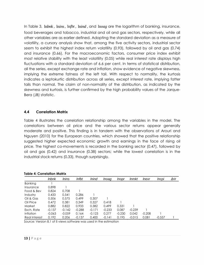
4.4 Correlation Matrix
Table 4 illustrates the correlation relationship among the variables in the model. The
correlations between oil price and the various sector returns appear generally
moderate and positive. This finding is in tandem with the observations of Arouri and
Nguyen (2010) for the European countries, which showed that the positive relationship
suggested higher expected economic growth and earnings in the face of rising oil
price. The highest co-movements is recorded in the banking sector (0.47), followed by
oil and gas (0.42) and insurance (0.38) sectors; while the lowest correlation is in the
industrial stock returns (0.33), though surprisingly.
Table 4: Correlation Matrix
lnbnk lnins lnfbt lnind lnoag lnopr lnmkt lnexr lncpi Δrir
Banking 1
Insurance 0.898 1
Food & Bev 0.824 0.708 1
Industry 0.433 0.541 0.286 1
Oil & Gas 0.506 0.575 0.499 0.307 1
Oil Price 0.472 0.381 0.349 0.327 0.418 1
Market 0.882 0.822 0.933 0.382 0.499 0.331 1
Exch. Rate -0.137 -0.142 -0.288 -0.171 -0.233 0.087 -0.239 1
Inflation -0.063 -0.059 0.164 -0.123 0.277 -0.230 0.042 -0.208 1
Real Interest 0.192 0.206 -0.137 0.400 -0.141 0.195 -0.015 0.081 -0.557 1
Source: Version 8.1 of E-views software was used in the estimation
14 | P a g e
An inverse relationship was observed between exchange rate and the various sector
returns, indicating a dampening effect of exchange rate depreciation on the
performance of the market. The positive relationship between exchange rate and oil
price shows the regime of appreciation as reserves are built up in the face of increasing
international oil price. Overall, there are positive co-movements between market
returns index and the sector returns of the food, beverages and tobacco, banking and
insurance, with 0.93, 0.88 and 0.82 correlation, respectively.
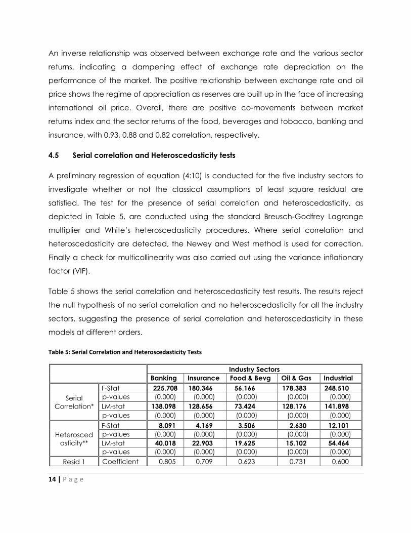
4.5 Serial correlation and Heteroscedasticity tests
A preliminary regression of equation (4:10) is conducted for the five industry sectors to
investigate whether or not the classical assumptions of least square residual are
satisfied. The test for the presence of serial correlation and heteroscedasticity, as
depicted in Table 5, are conducted using the standard Breusch-Godfrey Lagrange
multiplier and White’s heteroscedasticity procedures. Where serial correlation and
heteroscedasticity are detected, the Newey and West method is used for correction.
Finally a check for multicollinearity was also carried out using the variance inflationary
factor (VIF).
Table 5 shows the serial correlation and heteroscedasticity test results. The results reject
the null hypothesis of no serial correlation and no heteroscedasticity for all the industry
sectors, suggesting the presence of serial correlation and heteroscedasticity in these
models at different orders.
Table 5: Serial Correlation and Heteroscedasticity Tests
Industry Sectors
Banking Insurance Food & Bevg Oil & Gas Industrial
Serial
Correlation*
F-Stat 225.708 180.346 56.166 178.383 248.510
p-values (0.000) (0.000) (0.000) (0.000) (0.000)
LM-stat 138.098 128.656 73.424 128.176 141.898
p-values (0.000) (0.000) (0.000) (0.000) (0.000)
Heterosced
asticity**
F-Stat 8.091 4.169 3.506 2.630 12.101
p-values (0.000) (0.000) (0.000) (0.000) (0.000)
LM-stat 40.018 22.903 19.625 15.102 54.464
p-values (0.000) (0.000) (0.000) (0.000) (0.000)
Resid 1 Coefficient 0.805 0.709 0.623 0.731 0.600

15 | P a g e
Notes: *Breuch-Godfrey Langrange Multiplier Test, **White Heteroscedasticity test, excluding White Cross
terms. Source: Version 8.1 of E-views software was used in the estimation
These conclusions are drawn from the relatively high values of both the LM-stat and F-
stat and the small p-values that are less than 0.05 for a 95 per cent confidence interval,
which suggest the rejection of the null hypothesis of no serial correlation. It is also noted
that the first and second lagged residual terms are statistically significant at 5 per cent
significance level, indicating that serial correlation is of first and second order. The
rejection of the null hypothesis implies that economically, the variance of the
dependent variable across the data in the regressions is influenced by the volatility in oil
price. To correct for the bias that could be introduced by the observed autocorrelation
and heteroscedasticity in the models, the estimation procedures for standard errors and
p-values incorporated the HAC Newey-West (1987).
The check for the presence of multicollinearity, a common challenge with multifactor
modelling in the literature, the variance inflationary factor (VIF) was computed6. The
result indicates that the VIF values for all the macroeconomic factors, except market
index, are far from the restrictive critical value (VIF > 5). This implies that though
multicollinearity is present in the model, it is at a tolerable level and do not pose any
serious threat to the overall result.
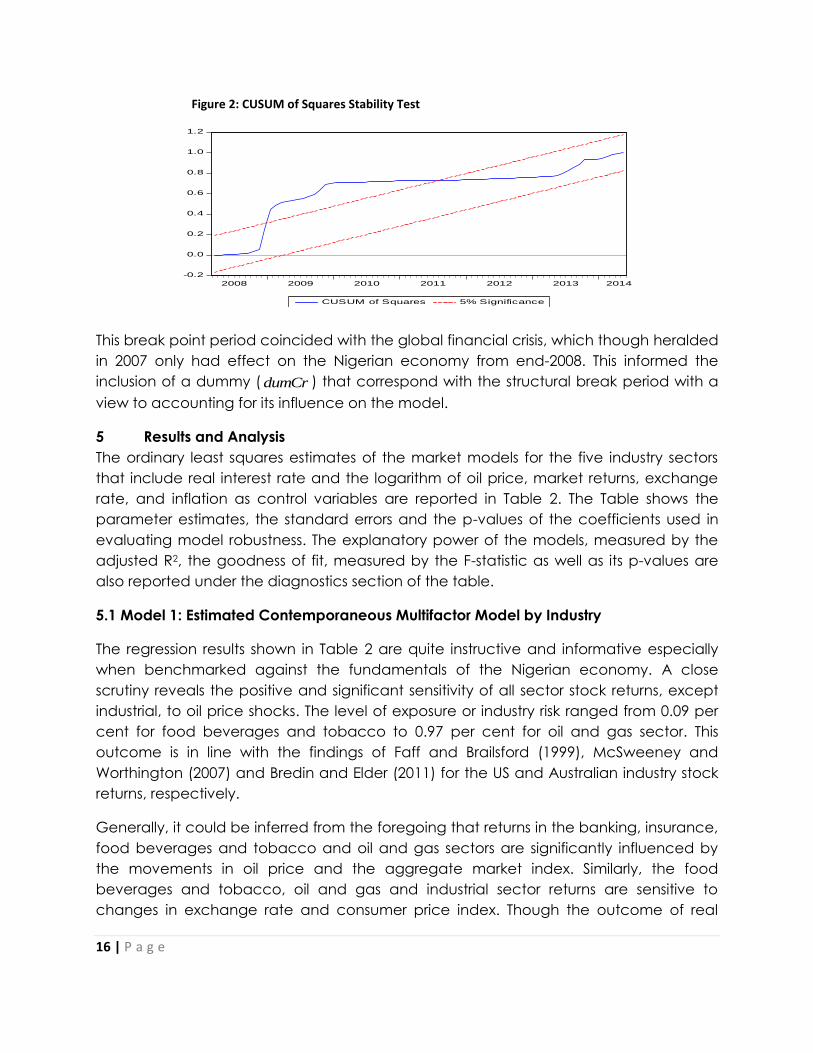
4.6 Structural Stability Test
The classical Chow (1960) structural stability test was conducted to detect evidence of
potential structural break. The CUSUM squared result presented in Figure 4 rejects the
hypothesis of coefficient stability at five per cent significance, suggesting the presence
of structural change in the model. This is an indication that, though most of the residuals
are within their confidence interval limits or bounds, structural breaks potentially occur
in the model at 2008M12 and lasted through 2011M07 during which point the residuals
drifted upward and departed from the confidence bands.
6 Variance Inflationary Factor is computed as 2
1
1VIF
R
where R2 is the unadjusted R-squared or correlation coefficient.
While there is no table of formal critical VIF values, a common rule of thumb is that if a given VIF is greater than 5, then
multicollinearity is severe and if it is less than 5, it is considered to be at a tolerable level. (Studenmund, 2011).
p-value (0.000) (0.000) (0.000) (0.000) (0.000)
Resid 2 Coefficient 0.047 0.130 -0.021 0.103 0.295
p-value (0.519) (0.066) (0.772) (0.161) (0.000)
16 | P a g e
Figure 2: CUSUM of Squares Stability Test
-0.2
0.0
0.2
0.4
0.6
0.8
1.0
1.2
2008 2009 2010 2011 2012 2013 2014
CUSUM of Squares 5% Significance
This break point period coincided with the global financial crisis, which though heralded
in 2007 only had effect on the Nigerian economy from end-2008. This informed the
inclusion of a dummy ( dumCr ) that correspond with the structural break period with a
view to accounting for its influence on the model.
5 Results and Analysis
The ordinary least squares estimates of the market models for the five industry sectors
that include real interest rate and the logarithm of oil price, market returns, exchange
rate, and inflation as control variables are reported in Table 2. The Table shows the
parameter estimates, the standard errors and the p-values of the coefficients used in
evaluating model robustness. The explanatory power of the models, measured by the
adjusted R2, the goodness of fit, measured by the F-statistic as well as its p-values are
also reported under the diagnostics section of the table.
5.1 Model 1: Estimated Contemporaneous Multifactor Model by Industry
The regression results shown in Table 2 are quite instructive and informative especially
when benchmarked against the fundamentals of the Nigerian economy. A close
scrutiny reveals the positive and significant sensitivity of all sector stock returns, except
industrial, to oil price shocks. The level of exposure or industry risk ranged from 0.09 per
cent for food beverages and tobacco to 0.97 per cent for oil and gas sector. This
outcome is in line with the findings of Faff and Brailsford (1999), McSweeney and
Worthington (2007) and Bredin and Elder (2011) for the US and Australian industry stock
returns, respectively.
Generally, it could be inferred from the foregoing that returns in the banking, insurance,
food beverages and tobacco and oil and gas sectors are significantly influenced by
the movements in oil price and the aggregate market index. Similarly, the food
beverages and tobacco, oil and gas and industrial sector returns are sensitive to
changes in exchange rate and consumer price index. Though the outcome of real
17 | P a g e
interest rate are mixed, all sectors except the oil and gas, respond significantly to
movements in real interest rate. The estimates also show that the dummy variable
tracking the effect of the global financial crisis is significant for all the sectors except
industrial sectors with the impact being more on the insurance and oil and gas sectors.
These conclusions are affirmed by the adjusted R2. The explanatory power of the
models was adjudged to be very adequate as the ability of the models to explain the
sensitivity of stock returns vary from 34 per cent for the industrial sector to 92 per cent for
food beverages and tobacco sector. The F-statistics with the associated p-values
indicate the goodness of fit of the models.
The dummy variable introduced to capture the effect of the 2007 global financial crisis
satisfies the apriori expectation for three of the four sectors. The negative coefficients
are consistent with economic literature that hypothesises increased cost of production
during depressions or financial crisis periods. The increased cost of doing business, in
addition to contagion and panic selling, translates to a decline in cash flow as well as
prices and returns in the stock market. In Nigeria, this loss was as much as 46 per cent in
stock returns in 2008. Estimates suggest that the risks are highest for the insurance and
oil and gas sectors with 0.007 per cent each. Counterintuitively, the industrial sector that
depend highly on imported raw and intermediate materials, industrial equipment as
well as technology for productive purposes, show no response to global crisis. However,
the banking sector, with 0.02 per cent exhibits some measure of resilience to the global
crisis pressures, owing largely to the banking sector consolidation exercise embarked on
in 2004, and the subsequent huge bail outs and other intervention measures by the
central bank during the crisis. These interventions strengthened the capital base of
banks and insulated the sector from the full impact of the global turbulence until the
second round effect of the crisis in 2008.

18 | P a g e
Table 2: Regression Analysis of Multifactor Market Models by Industry
Model 1: Impact of Oil Price Change on Industry Stock Returns Model 2: Sensitivity Analysis of Industry Stock Return on Oil Price Change
Banking Insurance Food & Bevg Oil & Gas Industrial Banking Insurance Food & Bevg Oil & Gas Industrial
Constant
Coefficient -0.142* -0.201* -0.104* -0.513* -0.213 0.016 -0.068 -0.029 -0.413* -0.845*
Std Errors (0.081) (0.111) (0.034) (0.208) (0.222) (0.085) (0.151) (0.044) (0.231) (0.269)
p-values 0.079 0.072 0.002 0.014 0.339 0.852 0.654 0.504 0.076 0.002
LNOPR
Coefficient 0.274* 0.272* 0.089* 0.974* 0.479 0.307* 0.228 0.147* 0.912* 0.294
Std Errors (0.082) (0.110) (0.045) (0.252) (0.316) (0.072 (0.159) (0.055) (0.275) (0.321)
p-values 0.001 0.014 0.051 0.000 0.131 0.000 0.152 0.008 0.001 0.361
LNMKT
Coefficient 1.121* 1.230* 1.213* 0.403 0.807* 1.174* 1.475* 1.112* 0.657* 0.918*
Std Errors (0.103) (0.119) (0.039) (0.266) (0.369) (0.093) (0.143) (0.041) (0.272) (0.370)
p-values 0.000 0.000 0.000 0.131 0.030 0.000 0.000 0.000 0.016 0.014
LNEXR
Coefficient -0.037 -0.025 -0.046* -0.363* -0.330* -0.047 -0.059 -0.109* -0.375* 0.071
Std Errors (0.043) (0.070) (0.024) (0.138) (0.146) (0.018) (0.098) (0.025) (0.140) (0.092)
p-values 0.932 0.718 0.057 0.009 0.024 0.329 0.550 0.000 0.008 0.440
LNCPI
Coefficient 0.783 1.308 0.689* 5.286* 2.546 0.459 0.669 0.769* 4.683* 3.172*
Std Errors (0.717) (0.860) (0.259) (1.537) (1.710) (0.734) (1.126) (0.365) (1.544) (1.682)
p-values 0.276 0.130 0.008 0.001 0.138 0.532 0.553 0.036 0.002 0.061
RIR
Coefficient 0.015* -0.021* -0.005* -0.005 0.064* 0.016* 0.024* -0.005* -0.003 0.061*
Std Errors (0.005) (0.006) (0.003) (0.012) (0.020) 0.005 0.006 (0.002) 0.013 (0.017)
p-values 0.001 0.001 0.043 0.652 0.001 0.001 0.0002 0.006 0.832 0.0004
dumCr
Coefficient -0.002* -0.007* 0.002* -0.007* -0.001
Std Errors (0.001) (0.002) (0.001) (0.003) 0.006
p-values 0.0002 0.0003 0.005 0.005 0.924
dumF
Coefficient -0.003* -0.003* -0.001 -0.002 0.007*
Std Errors 0.007 (0.001) (0.0004) (0.0002) (0.002)
p-values 0.0001 0.010 0.119 0.275 0.0014
dumR
Coefficient -0.002* -0.003* -0.001 -0.002 0.011*
Std Errors 0.001 0.001 (0.0004) (0.002) (0.003)
p-values 0.002 0.015 0.114 0.220 0.001
Diagnostics
Adjusted R2 0.86 0.82 0.92 0.50 0.34 0.87 0.74 0.89 0.44 0.44
F-Stat 193.22 144.05 366.11 33.92 17.48 181.87 80.95 249.91 22.62 22.43
p-value 0.000 0.000 0.000 0.000 0.000 0.000 0.000 0.000 0.000 0.000
Wald Test (2 ) 0.0002 0.0000 0.0211 0.9805 0.0011

19 | P a g e
5.2 Model 2: Examining the Sensitivities of Industry Returns on Oil Price Changes
To measure the degree of sensitivity of the five industry stock returns to upward or
downward swings in oil price, equation (4.12) was estimated to include two interactive
dummies ( dumR and dumF ) to capture the swings, respectively. The five estimated
dynamic regression models for the entire sample period, along with the coefficients
and standard errors, are presented as model 2 on the right hand side of Table 2.
Regression results indicate general consistency with the theoretical expectations in the
literature, albeit some exceptions. Specifically, the sensitivity of the industry stock returns
to oil price spike and declines, as measured by the interactive dummies, was largely
asymmetric as the risk factors for both the up or downward movements trended in the
same direction. For instance, both price rise and fall measured by dumR and dumF ,
respectively, exert negative and statistically significant impact on the banking and
insurance, but a positive effect on industrial sector stock returns. The negative impact is
in consonance with the literature (Sadorsky 2001, and IMF (2000), which generally
associated oil price increase with rising cost of production and weakening firms’ profit
margin. The implication is that a contemporaneous increase in oil price hikes firms’
production cost, erodes their cash flow positions, decreases investment and eventually
diminishes the firm’s returns on stocks through lower stock prices.
The outcomes of a fall in oil price, measured by interactive variable dumF,
counterintuitively replicate the dumR trend. This could be explained by the concept of
downward stickiness of prices, a common incidence in economic literature, which
assumes the willingness of some firms in an economy to adjust their prices during any
given period, and the reluctance of some others due to fixed costs associated with the
price change. This concept typifies the persistence of the inherently rigid oil price in
Nigeria which, very often, responds swiftly to price rise but very sluggishly to price
decline. In addition, the result also attests to the effects of petroleum subsidy
programme that insulates domestic consumers from oil price fluctuations.
On the other hand, the industrial sector response to oil price change is asymmetric,
suggesting that an increase in oil price improve the stock returns of the sector rather
than diminish it. The positive significance is supported by the findings of Agusman and
Deriantino (2008), which noted that though oil price increase generally brought about
increased production cost and losses for investors, a decreasing oil price, to a large
extent, did not simultaneously result in increased returns. Interestingly the food
beverage and tobacco and oil and gas sectors show no sensitivity to oil price shocks. It
is expected that changes in oil price should influence household expenditure profile via
the weight of energy expenditure in the consumption basket of an average household.
This is, however, not the case for Nigeria as households are shielded from international
oil price shocks by the subsidy on petroleum and other related products in the country.

20 | P a g e
To test for asymptotic response for positive or negative oil price changes, the Wald chi-
squared test was conducted and is reported along with other diagnostics in Table 2.
With the null hypothesis stated as 6 7:Ho at 5 per cent significant level, the
computed value of chi-squared for all the sectors, except oil and gas, fail to reject the
null hypothesis, suggesting that price rise or fall makes significant difference in the
market. However, for the oil and gas sector, the null hypothesis is rejected, concluding
that there is no significant difference when the conjectures of oil price rise or fall are
tested.
5.3 Model 3: Estimated Dynamic Market Model with Contemporaneous and Lagged Oil
Dependencies by Industry
Finally, a dynamic regression model is estimated to determine the relative persistence
of oil price shock for each of the industry sector in the system. Included in the model are
market returns, the change in contemporaneous oil price and twelve lags of oil price
changes. Estimates for each of the five industry sectors are made with the inclusion of
the dummy capturing the financial and economic crisis of 2007 and the Newey and
West (1987) heteroscedasticity and autocorrelation consistent standard errors.
An abridged version of the result of Table 1A in the appendix, is presented as Table 3
showing the estimated coefficient and standard errors (in parenthesis) for the five
industries7. Inference from the Table shows that the banking, insurance and food
beverage and tobacco sectors display significant contemporaneous oil price effect.
The food beverage and tobacco also show significant lag effect at one and twelve
months, which according to McSweeney and Worthington (2007), suggests the
persistence of oil price shock in the industry. Other industries that exhibit persistence in
oil price shocks include insurance (four-month lag), oil and gas (four and six-month lags)
and industrial sector (four month lag). The implication is that apart from the
contemporaneous impact, it takes approximately four months for the impulse of a price
change to ultimately manifest on the sectoral activities in the market. This means that
industries are more influenced by the previous four months change in oil price than the
previous two or three months, suggesting the approximate cycle of time it takes for the
impact of oil price change to transmit through the economy.
7 See the full result presentation in Table 1A at the appendix

21 | P a g e
Table 3: Persistence Measurement in the Market
Notes: Version 8.1 of Eviews software was used in the estimation process. All regressions incorporate
Newey and West (1987) heteroscedasticity and autocorrelation consistent standard errors. The lags
are in months.
Two plausible explanations could be proffered; first crude oil sales are done mostly on
futures or forward trading contract and other trading windows that hedge against the
unpredictable international oil price, especially with the rising incidence of insecurity
and insurgence in the Middle East and other major oil producing states. Political, ethnic
and religious uprisings in these areas could adversely affect the world supply of crude.
Secondly, the recognition of the capricious nature of oil price, given the country’s
dependence on the resource, has informed various governments in Nigeria at different
times to build buffers or special accounts such as the Excess Crude Account and the
Sovereign Wealth Fund, where oil revenue earned in excess of the budget benchmark
is warehoused and invested to cushion the effect of future falling prices. It implies that it
takes approximately four months for oil price shock to filter through the economy
before impacting on the industry sectors in the economy. It could, therefore, be
deduced from the above that in Nigeria oil price shock have two major episodes of
impact, one at the contemporaneous and the other at four month lagged
dependencies.
Banking Insurance Food & Bevg Oil & Gas Industrial
Constant Coefficient -0.124* -0.157* -0.033* -0.124* -0.164
Std Errors (0.036) (0.056) (0.023) (0.086) (0.159)
LNMKT Coefficient 1.150* 1.272* 1.280* 0.721* 0.803*
Std Errors (0.096) (0.116) (0.051) (0.291) (0.369)
LNOPR Coefficient 0.307* 0.503* -0.210* 0.597 0.294
Std Errors (0.132) (0.247) (0.109) (0.391) (0.540)
LNOPR(-1) Coefficient 0.093 -0.229 0.205* -0.289 -0.205
Std Errors (0.121) (0.192) (0.112) (0.342) (0.405)
LNOPR(-4) Coefficient 0.022 0.379* -0.021 0.617* 0.724*
Std Errors (0.957) (0.162) (0.085) (0.324) (0.353)
LNOPR(-6) Coefficient -0.002 0.205 0.076 0.519* 0.852
Std Errors (0.080) (0.157) (0.092) (0.282) (0.558)
LNOPR(-12) Coefficient 0.101 0.322 -0.165* 0.257 0.477
Std Errors (0.153) (0.230) (0.099) (0.322) (0.680)
dumCr Coefficient -0.001* -0.006* 0.003* -0.003* 0.003
Std Errors (0.001) (0.002) (0.001) (0.002) (0.006)
Diagnostics
Adjusted R2 0.88 0.83 0.90 0.41 0.32
F-Statistics 90.86 59.63 109.89 9.37 6.73

22 | P a g e
6.0 Summary and Conclusion
This study used monthly data spanning 1997 to May 2014 for industry level analysis of the
impact of changes in oil price on stock returns in Nigeria. The motivation was informed
by the absence of industry level studies, even though several studies have been
conducted on the impact of oil price on the activities of the stock market in Nigeria. In
other words, the study tilts away from the traditional aggregate approach to the
analysis of investigating the impact of oil price shocks to the individual sector method
with the prime objective of eliciting some fundamental information that could have
been subsumed under the macro approach. Five industry sectors were examined
based on availability of data while the included macroeconomic factors were selected
guided by economic theory and existing literature. The overall results suggest that
changes in oil prices affect returns of all the sectors, except food beverages and
tobacco. This is unique for now.
The plausible explanation for the pronounced sensitivity of the various industries to oil
price factor may not be unconnected with the overt dependence of the economy on
oil export for foreign exchange earnings. Consistent with the findings of McSweeney
and Worthington (2007) and Agusman and Deriantino (2008) for the Australian and
Indonesian stock markets, respectively, the parameter estimates of market returns for
the banking, insurance, food beverages and tobacco, oil and gas and industrial
sectors significantly exceeded unity, suggesting the higher risk of these sectors vis-à-vis
market returns. The food beverages and tobacco and oil and gas sectors exhibit
significantly negative sensitivity to exchange rate risk, indicating that the depreciation
of the domestic currency severely hurt the returns of both sectors more than others,
especially for high import-dependent countries like Nigeria.
The implications of the above results are enormous and should be carefully considered
by policymakers in the formulation of policy. First, the negative response of all the
sectors to exchange rate movement calls for prudent management plus informed and
timely intervention in the market by the monetary authority to keep the rate stable. A
stable rate is a precursor for stable inflation rate and will enable planning especially as
an import dependent economy. It is also a clarion call for the development of the local
alternatives for imports in order to lessen the dependence of the economy.
The positive response of the banking sector to real interest rate shocks is a pointer to
economy managers that the grip on inflation rate must be firm. A high inflation rate
usually prompts the central bank to raise its base rate (monetary policy rate) upon
which the banking system interest rates are anchored. This is critical to the achievement
of the plausible inclusive growth objective of government.

23 | P a g e
Another significant implication of the result is the impact of the financial and economic
crisis dummy, which exerts a general depression in the market. This is a signal for the
economy to expand its foreign exchange earnings base by divesting to other sectors
like the processing of agricultural products for exports. This will drastically reduce the
vulnerability of the economy to global vagaries and forestall or better still minimize
future crisis.
Finally, the insensitivity of the food beverages and tobacco to oil price movement is an
indication of the inefficiency instituted by the subsidy on petroleum products that
insulate domestic consumption from fluctuations in oil prices. Subsidies distort the
efficient allocation of resources by the market and in the case of Nigeria abet and aid
corruption. The endless tales of abuses and mismanagement of the programme over
the decades attest to the need for government to have a holistic rethink of the subsidy
policy. More so, the original intention of the subsidy programme which was to serve as a
safety net for the less privilege in the society as well as protect the industrial sector from
the vicissitudes of the oil market has abinitio been defeated.
24 | P a g e
References
Adebiyi, M.A.; A. O. Adenuga, M. O. Abeng, and P. N. Omanukwue (2009), Oil Price Shocks,
Exchange Rate and Stock Market Behaviour: Empirical Evidence from Nigeria”. Joint
Paper presented at the 14th Annual Conference of African Econometric Society at Abuja
Sheraton Hotel and Towers, Abuja
Afshar, T. A., G. Arabian and R. Zomorrodian (2008), “Oil Price Shocks and the U.S Stock Market”,
2008 IABR & TLC Conference Proceedings San Juan, Puerto Rico, USA
Agren, M. (2006) “Does Oil Price Uncertainty Transmit To Stock Markets?”, Department of
Economics, Uppsala University, Sweden, Working paper 2006:23
Agusman, A. and E. Deriantino (2008), “Oil Price and Industry Stock Returns: Evidence from
Indonesia”, 21st Austrailian Finance and Banking Conference Paper Akpan, E. O. (2009) ‘Oil Price Shocks and Nigeria’s Macroeconomy’. A paper presented at the
2009 Annual Conference of the Centre for the Studies of African Economies, Held in
Oxford, UK. Paper no. 252.
Aliyu, S.U.R. (2009) ‘Oil Price Shocks and the Macroeconomy of Nigeria: A Non-Linear Approach’.
Munich Personal RePEc Achive (MPRA) Paper No. 18726, November
Ayadi, O.F., A. Chatterjee, and C.P. Obi (2000), “A Vector Autoregressive Analysis of an Oil-
Dependent Emerging Economy — Nigeria” OPEC Review, pp. 330–349.
Ayadi, O.F. (2005), “Oil Price Fluctuations and the Nigerian Economy” OPEC Review, pp. 199–217.
Arouri, M. H. and D. K. Nguyen (2010), “Oil Prices, Stock Markets and Portfolio Investment:
Evidence from Sector Analysis in Europe over the Last Decade,” Working Papers hal-
00507823, HAL.
Asteriou, D. and S. Hall (2007), “Applied Econometrics: A Modern Approach”, Palgrave
Macmillan, New York.
Balaz, P. and A. Londarev (2006), “Oil and its Position in the Process of Globalization of the World
Economy”. Politicka Ekonomie 54 (4), 508-528.
Basher, S.A. and P. Sadorsky, (2006). “Oil Price Risk and Emerging Stock Markets.” Global Finance
Journal, 17, p: 224–251.
BP (2014), “The BP Statistical Review of World Energy (2014)” bp.com/statisticalreview.
Bredin, D. and J. Elder (2011), “U.S. Oil Price Exposure: The Industry Effects”, UCD Geary Institute
Discussion Paper Series, WP2011/07
Broadstock, D. C., H. Cao and D. Zhang (2012), “Oil Shocks and their Impact on Energy Related
Stocks in China”, Energy Economics, Volume 34, Issue 6, November, 1888 – 1895.

25 | P a g e
CBN, (2010a) Annual Report and Statement of Accounts for the Year Ended 31st December,
Central Bank of Nigeria.
CBN, (2010b), “The Changing Structure of the Nigeria Economy”, Eds Charles N. O. Mordi,
Abwaku Englama and Banji S. Adebusuyi. Research Department, Central Bank of
Nigeria.
Chan, H. and R. Faff (1998) “The Sensitivity of Australian Industry Equity Returns to a Gold Price
Factor”. Accounting an d Finance, 38(2), 223-244
Chen, N. H., R. Roll and S. A. Ross (1986), “Economic Forces and the Stock Market”, Journal of
Business 59(3), 383 – 403
Chittedi, K. R. (2012), “Do Oil Prices Matters for India Stock Market? An Empirical Analysis”,
Journal of Applied Economics and Business Research 2(1): 2-10. Chow, G. C. (1960) Test of Equality between sets of coefficients in Two Linear Regressions.
Econometrica 28(3), 591-605
Cong, R. G, Y. M, Wei, J. L. Jiao, and Y. Fan, (2008). “Relationships between oil price shocks and
stock market: An empirical analysis from China.” Energy Policy, Vol 36, Issue 9.
Driesprong, G., B. Jacobson and B. Maat (2004), “Stock Markets and Oil Prices”, A paper
presented at Maasey University, Auckland, New Zealand, February.
Elsharif, I. D. Brown, B. Burton, B. Nixon and A. Russel (2005) Evidence on the Nature and extent of
the relationship between oil and equity value in UK. Energy Economics, 27, 819-830
Eryigit, M. (2009) “Effects of Oil Price Changes on the Sector Indices of Istanbul Stock Exchange”
International Research Journal of Finance and Economics Issue 25, pp 209-216.
Faff, R. and T. Brailsford (1999), “Oil Price Risk and the Australian Stock Market”, Journal of Energy
Finance and Development, 4(1), pp69 – 87.
Fama, E. F. (1970), “Efficient Exchange Market: A Review of Empirical Market”, Journal of
Finance, May 25:2, pp 383 – 417
Fama, E. F. (1981) “Stock Returns, Real Activity, Inflation and Money”, The American Economic
Review, Vol 71, No 4, 545-565, September.
Fan, Q. and M. Jahan-Parvar (2011), “U.S. Industry-Level Returns and Oil Price,” International
Review of Economics and Finance. Volume 22(1), pp112 – 128.
Gisser, M. and T. H. Goodwin (1986) “Crude oil and the Macroeconomy: Tests of some popular
notions”, J. Money Credit Banking 18 1, pp. 95-103
Gogineni, S. (2007), “The Stock Market Reaction to Oil Price Changes,” Working
Paper, University of Oklahoma.
----------------- (2010), “Oil and the Stock Market: An Industry Level Analysis”, The Financial Review,
Volume 45, Issue 4, pp 995 – 1010.

26 | P a g e
Hamilton, J. D. (1983) “Oil and the Macroeconomy since World War II,” Journal of Political
Economy, 91, 228-248. Huang, R. D., R.W. Masulis and H. R. Stoll (1996). Energy Shocks and Financial Markets. Journal of
Futures Markets, 16, 1−27.
Iwayemi, A. and B. Fowowe (2010) ‘Impact of Oil Price Shocks on Selected Macroeconomic
Variables in Nigeria’. Energy Policy, Vol. 39, pp603-612 IMF (2000), “The Impact of Higher Oil Prices on the Global Economy”. A Paper Prepared by the
Research Department, International Monetary Fund, December
Jones, C. and G. Kaul (1996), “Oil and the stock markets”, Journal of Finance 51, 2, 463-91. Jones, D.W., P.N. Lelby, and I.K. Paik (2004), “Oil Price Shocks and the Macro-economy: What
Has Been Learned since 1996?” Energy Journal, 25, 1–32.
Khoo, A. (1994) “Estimation of Foreign Exchange Exposure: An Application to Mining Companies
in Australia”. Journal of International Money and Finance, 13(3), 342-363
Kilian, L. (2007) “The Economic Effects of Energy Price Shocks”, invited by the Journal of
Economic Literature.
Kilian, L. and C. Park (2008) “The Impact of Oil Price Shocks on the U.S. Stock Market”,
Department of Economics, University of Michigan and CEPR
Koranchelian, T. (2005) The Equilibrium Real Exchange Rate in a Commodity Exporting Country:
Algeria’s Experience. IMF Working Paper 05/135
Korhonen, I. and T. Juurikkala (2009) “Equilibrium exchange rates in oil-exporting countries”
Journal of Economics and Finance, Vol 33, No 1
Kim, I-M. and P. Loungani (1992) “The Role of Energy in Real Business Cycle Models”, Journal of
Monetary Economics, Elsevier, Vol 29(1) 173-189
Kwiatkowski, D., P. C. B. Phillips, P. Schmidt, and Y. Shin (1992) “Testing the Null Hypothesis of
Stationarity against Alternative of a Unit Root”. Journal of Econometrics, 54(1-3), 159-178
McCsweeney, E. J. and A. C. Worthington (2007), “A Comparative Analysis of Oil as a Risk Factor
in Australian Industry Stock Returns, 1980-2006” University of Wollongong, School of
Accounting and Finance Working Paper Series No. 07/07.
Mordi, C. N. O. and M. A. Adebiyi (2010), “The Asymmetric Effects of Oil Price Shocks on Output
and Prices in Nigeria using a Structural VAR Model”, Economic and Financial Review.
Volume 48 (1), March, pp 1-32.
Mork, K. A. (1989) “Oil Shocks and the Macroeconomy when Prices Go Up and Down: an
Extension of Hamilton’s Results,” Journal of Political Economy, 97 (51), No. 3, pp 740-744.
Nandha, M. and H. Singh (2011), “Oil Price and Stock Market Returns: The Chinese Market”, A
paper presented at the Second International Finance Conference at IIM Calcutta, India,
January

27 | P a g e
Nandha, M. and S. Hammoudeh (2007) “Systematic risk and oil price exchange rate sensitivities
in Asia Pacific stock markets”, Research in International Business and Finance 21 (2007) 326-
341
Nandha, M. and R. Faff (2008) “Does Oil Move Equity? A Global View”, Department of
Accounting and Finance, Monash University Australia. Energy Economics 30, 986-997.
Newey, W. and K. West (1987) A simple Positive Semi-Definite, Heteroscedasticity and
Autocorrelation Consistent Covariance Matrix. Econometrica 55, 703-708
Olomola, P.A and A.V. Adejumo (2006) “Oil Price shocks and Macroeconomic Activities in
Nigeria” International Research Journal of Finance and Economics, Issue 3, pp 28-34
Omisakin, O., O. Adeniyi and A. Omojolaibi (2009) ‘A Vector Error Correction Modelling of Energy
Price Volatility of an Oil Dependent Economy: The Case of Nigeria’, Pakistan Journal of
Social Sciences 6(4): 207-213
Papapetrou, E. (2009) “Oil Price Asymmetric Shocks and Economic Activity: The Case of
Greece”, University of Athens, Department of Economics, Athens, Greece and Bank of
Greece, Economic Research Department.
Park, J. W. and R. A. Ratti (2008) “Oil price shocks and Stock markets in the U.S. and 13 European
Countries” Energy Economics, 30, p: 2587–2608.
Rault C. and M. H. Arouri (2009) “Oil prices and stock markets: what drives what in the Gulf
Corporation Council countries? William Davidson Institute Working Paper Number 960 Rifkin, J. (2002). The hydrogen economy. New York Tarcher Putnam.
Sadorsky, P. (1999), “Oil Price Shocks and Stock Market Activity,” Energy Economics 21, 449-469.
Sadorsky, P. (2001), “Risk Factors in Stock Returns of Canadian Oil and Gas Companies. Energy
Economics, 23, 17-28
Sadorsky, P. and I. Henrques (2001), “Multifactor Risk and the Factor Returns of Canadian Paper
and Forest Products Companies”. Forest Policy Economics, 3(3-4), 199-208)
Sill, K. (2007) ‘The Macroeconomics of Oil Shocks’, Business Review Q1, Philadelphia Federal
Reserve Bank. www.philadelphiafed.org/econ/br/ index.html.
Studenmund, A. H. (2011), “Using Econometrics: A Practical Guide”. Pearson Addison-Wesley. 6th
Edition
Umar, G. and A. A. Kilishi (2010) ‘Oil Price Shocks and the Nigerian Economy: A Variance
Autoregressive (VAR) Model’. International Journal of Business and Management. Volume
5, No. 8, August.
Yurtsever, C. and T. Zahor (2007) “Oil Price Shocks and Stock Market in the Netherlands”,
University of Groningen, December

28 | P a g e
Appendix
Table 1A: Industry Analysis of Oil Price Shock Persistence in Nigeria
Model 3
Banking Insurance Food & Bevg Oil & Gas Industrial
Constant
Coefficient -0.124* -0.157* -0.033* -0.124* -0.164
Std Errors 0.036 0.056 0.023 0.086 0.159
p-values 0.008 0.005 0.152 0.151 0.304
LNMKT
Coefficient 1.150* 1.272* 1.280* 0.721* 0.803*
Std Errors 0.096 0.116 0.051 0.291 0.369
p-values 0.000 0.001 0.000 0.014 0.031
LNOPR
Coefficient 0.307* 0.503* -0.210* 0.597 0.294
Std Errors 0.132 0.247 0.109 0.391 0.540
p-values 0.021 0.044 0.057 0.128 0.587
LNOPR(-1)
Coefficient 0.093 -0.229 0.205* -0.289 -0.205
Std Errors 0.121 0.192 0.112 0.342 0.405
p-values 0.443 0.235 0.071 0.397 0.613
LNOPR(-2)
Coefficient 0.113 0.167 -0.001 0.150 0.389
Std Errors 0.106 0.168 0.085 0.291 0.325
p-values 0.287 0.321 0.986 0.606 0.233
LNOPR(-3)
Coefficient -0.052 -0.079 0.023 -0.305 -0.104
Std Errors 0.906 0.171 0.079 0.266 0.458
p-values 0.570 0.645 0.769 0.253 0.821
LNOPR(-4)
Coefficient 0.022 0.379* -0.021 0.617* 0.724*
Std Errors 0.957 0.162 0.085 0.324 0.353
p-values 0.815 0.021 0.804 0.058 0.041
LNOPR(-5)
Coefficient -0.024 -0.273 -0.107 0.127 -0.194
Std Errors 0.098 0.170 0.098 0.290 0.357
p-values 0.803 0.111 0.278 0.662 0.587
LNOPR(-6)
Coefficient -0.002 0.205 0.076 0.519* 0.852
Std Errors 0.080 0.157 0.092 0.282 0.558
p-values 0.978 0.193 0.407 0.068 0.129

29 | P a g e
Table 1A: Industry Analysis of Oil Price Shock Persistence in Nigeria (contd)
Notes: Eviews 8 software was used in the estimation. All regressions incorporate Newey and West (1987)
heteroscedasticity and autocorrelation consistent standard errors. The lags are in months.
Banking Insurance Food & Bevg Oil & Gas Industrial
LNOPR(-7)
Coefficient 0.056 0.026 0.019 -0.303 -0.384
Std Errors 0.091 0.163 0.078 0.352 0.436
p-values 0.539 0.872 0.805 0.389 0.379
LNOPR(-8)
Coefficient -0.036 -0.141 -0.001 0.222 0.129
Std Errors 0.086 0.147 0.081 0.327 0.499
p-values 0.677 0.338 0.992 0.498 0.796
LNOPR(-9)
Coefficient 0.048 -0.019 0.133 -0.203 -0.113
Std Errors 0.076 0.139 0.086 0.302 0.359
p-values 0.530 0.891 0.122 0.503 0.753
LNOPR(-10)
Coefficient 0.027 -0.045 -0.036 0.058 0.159
Std Errors 0.079 0.136 0.078 0.268 0.301
p-values 0.734 0.742 0.645 0.828 0.597
LNOPR(-11)
Coefficient -0.071 -0.063 0.005 -0.164 -0.099
Std Errors 0.127 0.172 0.087 0.321 0.393
p-values 0.576 0.714 0.951 0.610 0.800
LNOPR(-12)
Coefficient 0.101 0.322 -0.165* 0.257 0.477
Std Errors 0.153 0.230 0.099 0.322 0.680
p-values 0.512 0.165 0.098 0.426 0.484
dumCr
Coefficient -0.001* -0.006* 0.003* -0.003* 0.003
Std Errors 0.001 0.002 0.001 0.002 0.006
p-values 0.009 0.0004 0.0002 0.034 0.667
Diagnostics
Adjusted R2 0.88 0.83 0.90 0.41 0.32
F-Statistics 90.86 59.63 109.89 9.37 6.73
p-values 0.000 0.000 0.000 0.000 0.000