analysis of the arctic system for freshwater cycle

Analysis of the Arctic System for Freshwater Cycle Intensification:Observations and Expectations

MICHAEL A. RAWLINS,a,b MICHAEL STEELE,c MARIKA M. HOLLAND,d JENNIFER C. ADAM,e JESSICA

E. CHERRY,f JENNIFER A. FRANCIS,g PAVEL YA. GROISMAN,h LARRY D. HINZMAN,f THOMAS

G. HUNTINGTON,i DOUGLAS L. KANE,j JOHN S. KIMBALL,k RON KWOK,l RICHARD B. LAMMERS,m

CRAIG M. LEE,n DENNIS P. LETTENMAIER,o KYLE C. MCDONALD,l ERIKA PODEST,l JONATHAN

W. PUNDSACK,m BERT RUDELS,p MARK C. SERREZE,q ALEXANDER SHIKLOMANOV,m

ØYSTEIN SKAGSETH,r TARA J. TROY,s CHARLES J. VOROSMARTY,t MARK WENSNAHAN,c

ERIC F. WOOD,s REBECCA WOODGATE,c DAQING YANG,j KE ZHANG,k AND TINGJUN ZHANGq

a Department of Earth Sciences, Dartmouth College, Hanover, New Hampshirec Polar Science Center, Applied Physics Laboratory, University of Washington, Seattle, Washington

d National Center for Atmospheric Research, Boulder, Coloradoe Department of Civil and Environmental Engineering, Washington State University, Pullman, Washington

f International Arctic Research Center, University of Alaska Fairbanks, Fairbanks, Alaskag Institute of Marine and Coastal Sciences, Rutgers University, Highlands, New Jersey

h UCAR, National Climatic Data Center, Asheville, North Carolinai U.S. Geological Survey, Augusta, Maine

j Water and Environmental Research Center, Institute of Northern Engineering, University of Alaska

Fairbanks, Fairbanks, Alaskak Numerical Terradynamic Simulation Group, The University of Montana, Missoula, Montana

l Jet Propulsion Laboratory, California Institute of Technology, Pasadena, Californiam Water Systems Analysis Group, Institute for the Study of Earth, Oceans, and Space, University of New

Hampshire, Durham, New Hampshiren Ocean Physics Department, Applied Physics Laboratory, University of Washington,

Seattle, Washingtono Department of Civil and Environmental Engineering, University of Washington,

Seattle, Washingtonp Department of Physical Sciences, University of Helsinki, and Finnish Meteorological Institute,

Helsinki, Finlandq National Snow and Ice Data Center, Cooperative Institute for Research in Environmental Sciences,

University of Colorado, Boulder, Colorador Institute of Marine Research, and Bjerknes Centre for Climate Research, Bergen, Norway

s Department of Civil and Environmental Engineering, Princeton University, Princeton, New Jerseyt Department of Civil Engineering, The City University of New York, New York, New York

(Manuscript received 9 September 2009, in final form 1 June 2010)

ABSTRACT

Hydrologic cycle intensification is an expected manifestation of a warming climate. Although positive

trends in several global average quantities have been reported, no previous studies have documented broad

intensification across elements of the Arctic freshwater cycle (FWC). In this study, the authors examine the

character and quantitative significance of changes in annual precipitation, evapotranspiration, and river

discharge across the terrestrial pan-Arctic over the past several decades from observations and a suite of

b Current affiliation: Department of Geosciences, University of Massachusetts, Amherst, Massachusetts.

Corresponding author address: Michael A. Rawlins, Dept. of Geosciences, University of Massachusetts, Amherst, MA 01003.

E-mail: [email protected]

1 NOVEMBER 2010 R A W L I N S E T A L . 5715

DOI: 10.1175/2010JCLI3421.1

� 2010 American Meteorological Society

coupled general circulation models (GCMs). Trends in freshwater flux and storage derived from observations

across the Arctic Ocean and surrounding seas are also described.

With few exceptions, precipitation, evapotranspiration, and river discharge fluxes from observations and

the GCMs exhibit positive trends. Significant positive trends above the 90% confidence level, however, are

not present for all of the observations. Greater confidence in the GCM trends arises through lower in-

terannual variability relative to trend magnitude. Put another way, intrinsic variability in the observations

tends to limit confidence in trend robustness. Ocean fluxes are less certain, primarily because of the lack of

long-term observations. Where available, salinity and volume flux data suggest some decrease in saltwater

inflow to the Barents Sea (i.e., a decrease in freshwater outflow) in recent decades. A decline in freshwater

storage across the central Arctic Ocean and suggestions that large-scale circulation plays a dominant role in

freshwater trends raise questions as to whether Arctic Ocean freshwater flows are intensifying. Although

oceanic fluxes of freshwater are highly variable and consistent trends are difficult to verify, the other com-

ponents of the Arctic FWC do show consistent positive trends over recent decades. The broad-scale increases

provide evidence that the Arctic FWC is experiencing intensification. Efforts that aim to develop an adequate

observation system are needed to reduce uncertainties and to detect and document ongoing changes in all

system components for further evidence of Arctic FWC intensification.

1. Introduction

Climatic warming has been greatest across northern

high latitudes in recent decades, and precipitation (P)

increases have been noted over some Arctic regions

(Berner et al. 2005). In its Fourth Assessment Report

(AR4), the Intergovernmental Panel on Climate Change

(IPCC) stated that ‘‘increases in the amount of pre-

cipitation are very likely in high latitudes’’ (Solomon

et al. 2007). This statement arises from model studies

that suggest climate warming will result in hydrologic

cycle ‘‘intensification.’’ But what is meant by the term

intensification and why do we expect these changes as

a result of warming?

Intensification is considered here to be an increase in

the freshwater (FW) fluxes between the Arctic’s atmo-

spheric, land, and ocean domains. Conceptually, inten-

sification can be illustrated by an arrow connecting two

boxes in a schematic diagram, where the boxes represent

stocks of water in these domains (e.g., see Fig. 4 in

Serreze et al. 2006). For any given flux (arrow) between

stocks (boxes), a more intense flux would be represented

by a larger arrow. More water is now moving between

or within the respective domains. For example, river

discharge (volume/time 5 flux) in 1999 was approxi-

mately 128 km3 yr21 greater than it was when mea-

surements began in the early 1930s (Peterson et al. 2002),

a trend of 2.0 km3 yr22. In our schematic diagram, the

arrow connecting the land to the ocean has increased

in size.

Why should water cycle intensification be expected?

Intensification is a critical aspect of the planetary re-

sponse to warming, related to the atmosphere’s ability

to hold more water as it warms as defined by the theo-

retical Clausius–Clapeyron relation. Allen and Ingram

(2002) noted that the Clausius–Clapeyron relation pre-

dicts that tropospheric moisture loading would result in

precipitation increasing by about 6.5% K21 of warming.

Climate models, however, predict a substantially weaker

sensitivity to warming on the order of 1%–3.4% K21

because of constraints in the exchange of mass between

the boundary layer and the midtroposphere (Held and

Soden 2006; Lambert and Webb 2008). Recent analyses

have indicated that surface specific humidity (Willett

et al. 2008) and total atmospheric water content, pre-

cipitation, and evaporation (Wentz et al. 2007) appear to

be increasing at rates more consistent with the Clausius–

Clapeyron equation than those predicted by general

circulation models (GCMs). This question, related to

sensitivity of the hydrologic system to warming, is of key

importance for understanding future climatic responses,

as water vapor is itself a greenhouse gas that acts as a

feedback to amplify temperature change forced by an-

thropogenic increases in CO2 and CH4. Intensification is

also likely to result in alterations of the hydrologic cycle

in terms of the geographic distribution, amount, and

intensity of precipitation that may lead to more flooding

and drought. Finally, increases in atmospheric water

vapor content will likely exacerbate heat stress (Gaffen

and Ross 1998) and increase stomatal conductance (Wang

et al. 2009).

Simulations with GCMs suggest future increases in

pan-Arctic precipitation and evapotranspiration (ET;

Holland et al. 2006; Kattsov et al. 2007), with the pre-

cipitation increases expected to outpace increases in

evapotranspiration, resulting in an upward trend in net

precipitation (P 2 ET) over time. Indeed, an analysis of

simulated changes from 10 models included in IPCC

AR4 for the years 1950–2050 found a consistent accel-

eration of the Arctic hydrologic cycle as expressed by an

increase in the fluxes of net precipitation, river runoff,

and net ice melt passing through the Arctic’s atmo-

spheric, land, and ocean domains (Holland et al. 2007).

Other model experiments suggest increased probabilities

5716 J O U R N A L O F C L I M A T E VOLUME 23

this century for quantities such as winter precipitation,

including its intensity and the number of ‘‘heavy’’ precip-

itation events across northern Eurasia (Khon et al. 2007).

Studies describing global trends suggest that intensifi-

cation may be occurring. A recent review by Huntington

(2006) lists precipitation, evapotranspiration, and river

discharge among the quantities that are increasing. Re-

cent studies focusing on major river basins have shown

that evapotranspiration is increasing (Berbery and Barros

2002; Serreze et al. 2002; Walter et al. 2004; Park et al.

2008). Fernandes et al. (2007) have reported trends to-

ward increasing ET over Canada for the period 1960–

2000 based on in situ climate observations and a land

surface model (LSM). Satellite observations over the

last three decades have shown increases in precipitation,

ET, and atmospheric water vapor content on a global

scale (Wentz et al. 2007). Weak positive global trends

have been reported in recent decades for soil moisture

(Sheffield and Wood 2007) and precipitation recycling

(Dirmeyer and Brubaker 2007). However, Serreze et al.

(2002) found no trends in precipitation recycling ratio

for the Lena, Yenisey, Ob, or Mackenzie basins from

1960 to 1999. There is also growing evidence for an in-

crease in indices of precipitation extremes (Alexander

et al. 2006; Tebaldi et al. 2006). The eruption of Mount

Pinatubo and subsequent massive introduction of SO2

into the stratosphere in 1991 provided a natural exper-

iment in planetary cooling that resulted in a weakening

(dampening) of the global hydrologic cycle that is the

reverse analog to climate warming. In the 2 yr following

the eruption, there was a decrease in atmospheric water

content (Santer et al. 2007) and a decrease in precipi-

tation and continental discharge (Trenberth and Dai

2007). Across some regions of the Arctic, precipitation

increases have been as much as 15% over the last 100 yr

(Berner et al. 2005), with most of the trend having oc-

curred during winter within the last 40 yr (Bradley et al.

1987; Groisman et al. 1991; Hanssen-Bauer and Forland

1994). Long-term increases in pan-Arctic precipitation,

however, have not been established.

Substantial progress in our understanding and quan-

tification of the Arctic freshwater cycle (FWC) has been

made over the past decade. In 2000, a comprehensive,

integrated view of the Arctic Ocean freshwater budget

and potential future changes were presented in ‘‘The

Freshwater Budget of the Arctic Ocean’’ (Lewis 2000).

Other studies have described changes in the Arctic

FWC (Peterson et al. 2002, 2006), quantified the mean

freshwater budget (Serreze et al. 2006), and examined

freshwater components depicted within coupled models

(Kattsov et al. 2007; Holland et al. 2007). Linkages be-

tween freshening of polar oceans and an intensifying

Arctic FWC have also been posited (Dickson et al. 2002;

Curry et al. 2003; Peterson et al. 2006). In a study ex-

amining 925 of the world’s largest ocean-reaching rivers,

Dai et al. (2009) showed that rivers having statistically

significant downward trends (45) outnumber those with

upward trends (19). However, for large Arctic rivers,

they report a large upward trend in annual discharge

into the Arctic Ocean from 1948 to 2004. Nonetheless,

Polyakov et al. (2008) and others have found that the

historical data indicate a decrease in Arctic Ocean fresh-

water storage. While the slow but steady increase in river

discharge might be expected to eventually increase ocean

freshwater storage and export to the south, the magnitude

and time scale of this forcing can be easily overwhelmed

by advective exchanges between ocean regions.

This paper presents a systematic analysis of change in

the Arctic FWC through a comparison of trends drawn

from observations and a suite of GCM simulations. We

focus on the sign and magnitude of change in fluxes such

as precipitation, river discharge, and liquid freshwater

transport in the Arctic Ocean. Section 2 is an overview

of the GCMs used in our analysis. Section 3 describes the

terrestrial observations, reanalysis data, and associated

trends. Section 4 is a synthesis of Arctic Ocean FWC

components. Results are summarized in Section 5. This

study builds on previous studies supported under the

National Science Foundation Arctic System Science

Freshwater Integration study (FWI), which have quan-

tified the large-scale freshwater budget (Serreze et al.

2006), characterized freshwater anomalies within the

Mackenzie River basin and the Beaufort Gyre (Rawlins

et al. 2009a), documented changes and feedbacks in the

freshwater system (White et al. 2007; Francis et al. 2009),

and described projected freshwater changes over the

twenty-first century (Holland et al. 2007).

2. General circulation models

Variability and trends in the Arctic FWC are drawn

from nine models examined in the World Climate Re-

search Programme’s (WCRP’s) Coupled Model Inter-

comparison Project phase 3 (CMIP3) multimodel dataset

(Table 1). These models were also part of IPCC AR4

(Solomon et al. 2007). Details of the model character-

istics and forcings are described in Holland et al. (2007),

who selected this model subset given their ability to re-

solve the passage of water through the Bering and Fram

Straits. Outputs examined here are from each model

control run of twentieth-century climate followed by

future simulations using the Special Report on Emis-

sions Scenarios (SRES) A1B scenario. In addition to

these nine models, Holland et al. also examined output

from the Goddard Institute for Space Studies Model E-R

(GISS E-R), which we do not use given known problems


in its depictions of observed climate over the region of

interest (Gorodetskaya et al. 2008; Holland et al. 2010).

In the analysis to follow, a time series for each model

represents a single model simulation, as not all models

had multiple ensemble members. Holland et al. (2007)

examined results across a terrestrial Arctic drainage

region, which included the large Eurasian river basins

(Ob, Yenesei, and Lena), the Mackenzie basin in North

America, and northern parts of Alaska, Greenland, and

the Canadian Archipelago (light gray in Fig. 1). In the

present study, pan-Arctic averages for the observations

are determined over the larger region shown in Fig. 1

(light gray plus dark gray). We minimize the effect of

differing volumes by computing and presenting unit

depths for all budget and trend magnitudes. Holland

et al. (2007) contains additional details of the GCMs and

associated simulations.

One of the more interesting findings from Holland

et al. (2007) is an intensification of fluxes such as net

precipitation, river runoff, and export of liquid fresh-

water to lower latitudes. Holland et al. (2007) suggested

that net precipitation over the Arctic terrestrial drainage

increases from 1950 through 2050 by 16%, with most of

this change occurring after 2000. Although intensifica-

tion among the models is universal, the magnitude of

change ranges widely. Moreover, the change in terres-

trial net precipitation among the models is significantly

correlated with initial values. In other words, models

with higher initial net precipitation amounts generally

exhibit larger changes.

3. Terrestrial system

a. Precipitation

Several sources of data, averaged over the terrestrial

Arctic drainage basin (light gray plus dark gray in Fig. 1)

excluding Greenland, are used to characterize precipi-

tation trends and variability. This region and the smaller

Arctic domain used by Holland et al. (2007) and Serreze

et al. (2006) are shown in Fig. 1. Records derived largely

from interpolations of gauge observations come from

three sources; the Willmott–Matsuura (WM) archive

(Willmott and Matsuura 2009), the Climate Research

Unit (CRU) version 3.0 dataset (Climatic Research Unit

2009), and the data presented by Sheffield et al. (2006,

hereafter referred to as S06). The latter data (S06) is a 18,

3-hourly global meteorological forcings dataset from

1948 through 2000. The precipitation data were created

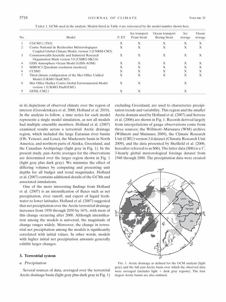
FIG. 1. Arctic drainage as defined for the GCM analysis (light

gray) and the full pan-Arctic basin over which the observed data

were averaged (includes light 1 dark gray regions). The four

largest Arctic basins are also outlined.

TABLE 1. GCMs used in the analysis. Models listed in Table 4 are referenced by the model number shown here.

No. Model P, ET

Ice transport

Fram Strait

Ocean transport

Bering Strait

Ice

storage

Ocean

storage

1 CGCM3.1 (T63) X X X X X

2 Centre National de Recherches Meteorologiques

Coupled Global Climate Model, version 3 (CNRM-CM3)

X X X X X

3 Commonwealth Scientific and Industrial Research

Organisation Mark version 3.0 (CSIRO Mk3.0)

X X X X X

4 GISS Atmosphere–Ocean Model (GISS-AOM) X X X X X

5 MIROC3.2[medium resolution (medres)] X X X X X

6 CCSM3 X X X X X

7 Third climate configuration of the Met Office Unified

Model (UKMO HadCM3)

X X X X X

8 Met Office Hadley Centre Global Environmental Model

version 1 (UKMO HadGEM1)

X X X

9 GFDL-CM2.1 X X X


by sampling the National Centers for Environmental

Prediction–National Center for Atmospheric Research

(NCEP–NCAR) reanalysis data for daily variability af-

ter correcting for rain-day anomalies across the high

latitudes. Monthly precipitation was scaled to match the

CRU version 2.0 dataset (Mitchell et al. 2004). Given

the monthly scaling, trends in S06 precipitation should

be equivalent to trends in CRU data. We use an updated

version of S06 that does not include undercatch cor-

rections but does incorporate improvements to relative

humidity estimates across the Arctic. Gridded precipi-

tation data are also drawn from the Global Precipitation

Climatology Project (GPCP). Established by the World

Climate Research Programme, the GPCP draws on data

from over 6000 rain gauge stations as well as satellite

geostationary and low-orbit infrared, passive microwave,

and sounding observations. Several GPCP products are

available. We examine here the monthly data on a

18 global grid. We also analyze precipitation from the

Global Precipitation Climatology Center’s (GPCC’s) data-

set that is based on a quality-controlled data product

optimized for the best spatial coverage and use in water

budget studies.

Precipitation and ET are also available from reanalysis,

a retrospective form of numerical weather prediction

(NWP). Reanalysis involves assimilation of observations

within a coupled atmospheric–land surface model and

produces time series of gridded atmospheric fields and

surface state variables in a consistent manner. The 40-yr

European Centre for Medium-Range Weather Forecasts

(ECMWF) Re-Analysis (ERA-40) archives precipitation

and ET along with other atmospheric fields and surface

state variables for the period 1948–2002 (Kalnay et al.

1996), although data since 1979 (the advent of modern

satellite data streams) are generally of higher quality

(Bromwich and Fogt 2004). More recently the ERA-

Interim project has created gridded fields for 1989–2005

with improvements from the ERA-40, including a four-

dimensional (4D) variational assimilation system and im-

proved global hydrologic cycle. Data from the ERA-40

reanalysis were recently used in a comprehensive anal-

ysis of the Arctic’s freshwater budget and variability

(Serreze et al. 2006). Mean terrestrial budget magni-

tudes from that analysis are compared with those from

our precipitation, ET, and river discharge data and from

which trends are derived.

Gridded fields in both WM and CRU archives were

produced through interpolations of precipitation obser-

vations, with the point data having originated from gauge

measurements. Relative to precipitation across temper-

ate regions, observations of precipitation over the ter-

restrial Arctic are more sparse and, moreover, subject

to considerable uncertainties. Two significant sources of

error make climate change analysis of precipitation par-

ticularly challenging. First, observations recorded at

gauges are subject to several errors, with undercatch,

particularly in the solid form, generally the greatest

(Groisman et al. 1991). Low biases are often as high as

80%–120% in winter across coastal regions with strong

winds (Bogdanova et al. 2002; Yang et al. 2005; Goodison

et al. 1998). These biases can also change over time. Raw

gauge observations used to create the WM and CRU

datasets are devoid of undercatch adjustments. Second,

direct observations across the Arctic are extremely

sparse and station closures have occurred since the

early 1990s (Schiermeier 2006). A changing configu-

ration of stations can also impart biases into temporal

trends derived from the historical station network (Keim

et al. 2005; Rawlins et al. 2006). Biases due to a chang-

ing station network are minimized by focusing on time

periods starting in 1950 when the station network was

less variable.

Trend analysis of pan-Arctic (excluding Greenland)

annual precipitation and other water budget terms is

accomplished using linear least squares regression and a

two-tailed significance test. The precipitation and other

annual time series examined contain minimal temporal

autocorrelation and no adjustments to the raw data are

made. Precipitation-trend-slope magnitudes range from

20.03 to 0.79 mm yr22, with two of the six observed

series showing upward trends above the 90% confi-

dence level (Table 2). A significant positive trend of

0.21 mm yr22 is noted with the CRU version 3.0 dataset

(Fig. 2, Table 2). Time series from both S06 and WM

effectively show no trend. Relatively low precipitation

magnitudes with these data (Table 3) are likely attrib-

utable to a lack of adjustments for gauge undercatch.

Both GPCP and GPCC data show positive tendencies

(0.74 and 0.43 mm yr22, respectively) over recent de-

cades, but they are both too short to yield significant

trends. ERA-Interim exhibits the largest (0.79 mm yr22,

significant) trend. It is interesting to note that precipi-

tation data available over the latter decades of the twen-

tieth century (GPCP, GPCC, and ERA-Interim) show

sharper increases than the longer records. All of the pre-

cipitation datasets have mean annual totals within 15%

of the best estimates described in Serreze et al. (2006)

from 1979 to 1993 (Table 3).

Figure 3a shows the precipitation time series (1950–

1999) from the nine GCMs, the linear trend fits, and the

multimodel mean trend. Trends are all positive, ranging

from 0.12 to 0.63 mm yr22, with a multimodel mean

trend of 0.37 mm yr22 (Fig. 4a; Table 4). Significant

increases are noted for all but the Community Climate

System Model, version 3 (CCSM3) and the Geophysical

Fluid Dynamics Laboratory Climate Model version 2.1


(GFDL CM2.1) models. Over the 100-yr period from

1950 to 2049, trends range from 0.24 to as much as

0.92 mm yr22, with the multimodel mean trend at

0.65 mm yr22 (Fig. 4b). This suggests an acceleration

over the latter 50 yr. Regarding significance, greater

confidence can be ascribed to the GCM precipitation

increases, compared to the observational data trends,

largely because of a combination of higher trend magni-

tudes and longer time periods relative to the interannual

variability as reflected by the respective coefficient of

variation (CV). This follows from principles of statistical

significance tests, in that the required sample size to de-

tect a particular change depends on the magnitude of the

change, variability of the data, and the nature of the test.

These influences are evident when comparing the GCM

trend magnitudes and CVs in Fig. 4 with those for the

observations in Table 2. Intermodel scatter in pan-Arctic

precipitation is likely related to process error such as

model parameterizations of relevant precipitation pro-

cesses, which often explain the spatial consistency in this

error term (Finnis et al. 2009).

An increase in extreme precipitation events is also

expected as the climate warms (Held and Soden 2006).

Precipitation data (Groisman et al. 2003, 2005; Tebaldi

et al. 2006) show an increase in heavy precipitation

events (.2s of the events with precipitation .0.5 mm)

over western Russia (308–808E) and northern Europe;

opposite tendencies have been noted for the Asian part

of northwestern Eurasia, with more droughts and stron-

ger and/or more frequent weather conducive to fires

(Groisman et al. 2007; Soja et al. 2007). A circumpolar

increase of 12% has occurred for heavy precipitation

events since 1950 for the region north of 508N, with most

of the increase having come from Eurasia, where an

increase in convective clouds during spring and summer

has been observed (Groisman et al. 2007). Yet, while

precipitation extremes are likely related to warming and

associated increases in atmospheric water vapor, simple

models suggest that they may not be expected to in-

crease at the rate given by Clausius–Clapeyron scaling

because of changes in the moist-adiabatic lapse rate,

which lowers the rate of the precipitation increases due

to warming (O’Gorman and Schneider 2009).

Spatial estimates of precipitation suffer from two sig-

nificant sources of uncertainty: gauge undercatch and a

sparse station network. How do the uncertainties re-

lated to network arrangement and gauge catch affect

FIG. 2. Annual precipitation for the full pan-Arctic drainage

basin (light 1 dark gray regions) shown in Fig. 1. Time series are

from CRU, the ERA-Interim dataset, the multimodel mean from

the nine GCMs, GPCP, GPCC, S06, and the WM dataset. See also

Tables 2 and 3 and section 3a. Linear least squares trend fit through

annual values is shown.

TABLE 2. Trends and CVs for terms of the terrestrial water

budget. Null hypothesis is no trend over the specified time period.

Slope and statistical significance are determined using linear least

squares regression and the Student’s t test. Terms significant at

p , 0.1 (90% confidence) are indicated in bold. Entries in each

section are ordered by length of record. Trends and CVs for in-

dividual GCMs are shown in Fig. 4.

Term

Time

period

Trend

(mm yr22) CV (%)

Precipitation

CRU version 3.0 1950–2006 0.21 2.8

WM 1950–2006 20.03 2.7

GCMs 1950–1999 0.37 —

S06 1950–1999 0.11 2.5

GPCP 1983–2005 0.74 3.2

GPCC 1983–2005 0.43 2.6

ERA-Interim 1989–2005 0.79 1.7

Evapotranspiration

GCMs 1950–1999 0.17 —

VIC 1950–1999 0.11 3.6

LSMsa 1980–1999 0.40 2.2

RSb 1983–2005 0.38 2.6

ERA-Interim 1989–2005 0.30 2.5

River Discharge

North Americac 1950–2005 0.40 9.5

North Americad 1950–2005 0.12 7.4

Hudson Bay 1950–2005 20.29 9.4

Pan-Arctic 1950–2004 0.23 4.5

Eurasiae 1950–2004 0.31 4.8

GCMs, P 2 ET 1950–1999 0.20 —

JRA-25, P 2 ET 1979–2007 0.35 4.5

P 2 ETf 1983–2005 0.36 5.6

P 2 ETg 1983–2005 0.05 5.8

a Model mean ET of LSMs from Slater et al. (2007).b ET estimated from remote sensing with AVHRR GIMMS data.c Excluding the drainage to Hudson Bay.d Including the drainage to Hudson Bay.e For the six largest Eurasian rivers.f ET estimated from GPCP P minus RS ET.g ET estimated from GPCC P minus RS ET.


the annual precipitation trends? One study of bias ad-

justment has suggested that precipitation trends are

higher after adjusting for gauge undercatch (Yang et al.

2005). However, Førland and Hanssen-Bauer (2000) ar-

gued that a warming climate is imparting a false positive

trend into the data records because of a more efficient

catch of liquid precipitation over time. An examination

of both the raw and adjusted (for undercatch) records

from the TD9813 archive of former USSR meteoro-

logical stations (National Climatic Data Center 2005),

from 1950 through 1999, reveals that bias adjustments

were greater during the earlier decades than the later

ones. Thus, undercatch adjustment could tend to reduce

the positive slopes presented in Fig. 2. The network bias,

on the other hand, is likely to have the opposite effect on

the annual precipitation trends. Station networks during

the early decades of the twentieth century were estab-

lished across more southern parts of the terrestrial

Arctic. In time, observations were established in the

colder and drier north. Regionally averaged precipi-

tation values from early arctic networks would thus tend

to show positive bias relative to values from more recent

arctic networks (Rawlins et al. 2006). Although the effect

from 1950 through 1999 is likely small (,10 mm yr21),

adjusting for the bias in network configuration would

likely increase the trend slopes shown in Fig. 2, an effect

opposite in sign to bias due to gauge undercatch. There

is also a tendency for gauges to be located at lower ele-

vations, causing an underestimation in precipitation in

areas where there are mountains and strong orographic

effects.

b. Evapotranspiration

Surface-based observations of ET across the pan-Arctic

are sparse. Among the active sites in the Ameriflux pro-

gram (available online at http://public.ornl.gov/ameriflux/

index.html), only three are located within the Arctic

TABLE 3. Mean magnitude of terms of the pan-Arctic terrestrial

water budget. Entries are ordered the same as in Table 2. Period

over which the quantities in each category are derived is shown in

each heading. The first row in each category lists the value of the

best estimate from Serreze et al. (2006) derived from the ERA-40

reanalysis.

Term Magnitude (mm yr21)

Precipitation, 1979–93

Serreze et al. 490

CRU V3 410

Willmott–Matsuura 420

GCMs 490

S06 430

GPCP 520

GPCC 420

ERA-Interim 510

Evapotranspiration, 1979–93

Serreze et al. 310

GCMs 270

VIC 150

LSMsa 210

RSb 230

ERA-Interim 280

River discharge, 1979–2001

Serreze et al. P 2 ET 180

North Americac 220

North Americad 230

Hudson Bay 250

Pan-Arctic 230

Eurasiae 230

GCMs, P 2 ET 220

JRA-25, P 2 ET 200

P 2 ETf 290

P 2 ETg 190

a Model mean ET of LSMs from Slater et al. (2007).b ET estimated from remote sensing with AVHRR-GIMMS data.c Excluding the drainage to Hudson Bay.d Including the drainage to Hudson Bay.e For the six largest Eurasian rivers.f ET estimated from GPCP P minus RS ET.g ET estimated from GPCC P minus RS ET.

FIG. 3. (a) Precipitation and (b) evapotranspiration averaged over

the terrestrial pan-Arctic 1950–99 from the nine GCMs (Table 1).

Linear least squares trend fit is shown for each model. The heavy

black line is the multimodel mean trend.


drainage of North America, each in northern Alaska.

Likewise, the Long-Term Ecological Research (LTER)

network contains two Arctic sites, again both in Alaska.

In situ ET measurement networks are similarly sparse

for the Eurasian portion of the pan-Arctic. Given this

data void, our analysis of ET trends involves informa-

tion from land surface models and remote sensing data.

ET is defined here as the total flux from all sources such

as open water evaporation, transpiration from vegeta-

tion, and sublimation from snow.

Eddy covariance measurements are the primary means

of observing turbulent, boundary layer ET fluxes. For

regional- and continental-scale studies, models forced

with time-varying climate data (e.g., precipitation and

air temperature) must be used. The Variable Infiltration

Capacity (VIC) hydrologic model (Liang et al. 1994) is

a large-scale land surface model that solves for closure

of the water and energy balance equations. It has been

used in a variety of studies, both globally and across the

pan-Arctic. ET is modeled using the Penman–Monteith

equation, with resistances adjusted to account for soil

moisture availability, temperature, radiation, and vapor

pressure deficit. VIC contains a frozen soils scheme and

a two-layer, physically based snow model (Cherkauer

FIG. 4. Trends in (top) precipitation and (bottom) evapotranspiration averaged over the terrestrial pan-Arctic

drainage basin for the periods (left) 1950–99 and (right) 1950–2049 from the nine GCMs. Filled rectangles represent the

trend slope magnitudes for the models with a significant trend. The dashed line in each panel marks the multimodel

mean trend magnitude. CV (in percent) for each GCM time series is indicated below the respective vertical bar.

TABLE 4. Trend magnitudes (mm yr22) for P, ET, and P 2 ET for the terrestrial pan-Arctic over the period 1950–99 from the nine

GCMs. Multimodel mean trend is shown in the last column, with the mean trend over the longer 1950–2049 period in (). Trends significant

at 90% confidence level are indicated in bold.

Field 1 2 3 4 5 6 7 8 9 Mean

P (Land) 0.42 0.28 0.33 0.42 0.32 0.25 0.63 0.53 0.12 0.37 (0.65)

ET (Land) 0.25 0.17 0.16 0.13 0.19 0.19 0.24 0.25 20.07 0.17 (0.31)

P 2 ET (Land) 0.16 0.10 0.17 0.29 0.13 0.06 0.39 0.28 0.19 0.20 (0.34)


et al. 2003). Model parameters are calibrated to match

large basin discharge. Simulations show that VIC stream-

flow estimates compare well to gauge observations across

northern Eurasia and North America. Trends in ET

were taken from a VIC simulation that was performed

at a 6-h time step over the pan-Arctic domain with

forcing from the S06 dataset. Annual total ET from a

suite of five LSMs (including the VIC model) forced

with data from the ERA-40 reanalysis (European Cen-

tre for Medium-Range Weather Forecasts 2002) are also

examined here for trends. The simulations were made

on a 100-km grid across the pan-Arctic drainage basin as

described by Slater et al. (2007). For each model, pan-

Arctic ET is derived from the spatial grids within the

Arctic drainage basin, with the mean model trend drawn

from the five-model ET averages.

Estimates of ET at regional and global scales are

also available through satellite remote sensing. These

methods are generally based on surface energy balance

partitioning among sensible heat, latent heat, and soil

heat–heat storage fluxes. For this study we derive remote

sensing (RS)-based ET (monthly, 1983–2005) using the

Penman–Monteith approach by incorporating biome-

specific environmental stress factors and satellite-derived

radiation and vegetation information (Mu et al. 2007;

Zhang et al. 2009). The model employs the National

Aeronautics and Space Administration–Global Energy

and Water Cycle Experiment (NASA–GEWEX) solar

radiation and albedo inputs, the Advanced Very High

Resolution Radiometer (AVHRR) Global Inventory

Modeling and Mapping Studies (GIMMS) normalized

difference vegetation index (NDVI), and regionally cor-

rected NCEP–NCAR reanalysis daily surface meteorol-

ogy (Zhang et al. 2008, 2009). The ET estimates, originally

produced at a daily time step and 8-km spatial resolution,

were reprojected to the National Snow and Ice Data

Center (NSIDC) 12.5-km-resolution Equal-Area Scal-

able Earth Grid (EASE-Grid).

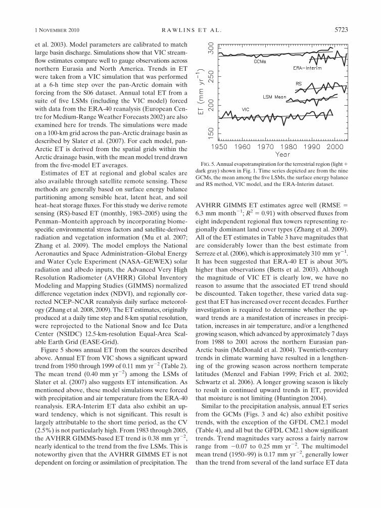
Figure 5 shows annual ET from the sources described

above. Annual ET from VIC shows a significant upward

trend from 1950 through 1999 of 0.11 mm yr22 (Table 2).

The mean trend (0.40 mm yr22) among the LSMs of

Slater et al. (2007) also suggests ET intensification. As

mentioned above, these model simulations were forced

with precipitation and air temperature from the ERA-40

reanalysis. ERA-Interim ET data also exhibit an up-

ward tendency, which is not significant. This result is

largely attributable to the short time period, as the CV

(2.5%) is not particularly high. From 1983 through 2005,

the AVHRR GIMMS-based ET trend is 0.38 mm yr22,

nearly identical to the trend from the five LSMs. This is

noteworthy given that the AVHRR GIMMS ET is not

dependent on forcing or assimilation of precipitation. The

AVHRR GIMMS ET estimates agree well (RMSE 5

6.3 mm month21; R2 5 0.91) with observed fluxes from

eight independent regional flux towers representing re-

gionally dominant land cover types (Zhang et al. 2009).

All of the ET estimates in Table 3 have magnitudes that

are considerably lower than the best estimate from

Serreze et al. (2006), which is approximately 310 mm yr21.

It has been suggested that ERA-40 ET is about 30%

higher than observations (Betts et al. 2003). Although

the magnitude of VIC ET is clearly low, we have no

reason to assume that the associated ET trend should

be discounted. Taken together, these varied data sug-

gest that ET has increased over recent decades. Further

investigation is required to determine whether the up-

ward trends are a manifestation of increases in precipi-

tation, increases in air temperature, and/or a lengthened

growing season, which advanced by approximately 7 days

from 1988 to 2001 across the northern Eurasian pan-

Arctic basin (McDonald et al. 2004). Twentieth-century

trends in climate warming have resulted in a lengthen-

ing of the growing season across northern temperate

latitudes (Menzel and Fabian 1999; Frich et al. 2002;

Schwartz et al. 2006). A longer growing season is likely

to result in continued upward trends in ET, provided

that moisture is not limiting (Huntington 2004).

Similar to the precipitation analysis, annual ET series

from the GCMs (Figs. 3 and 4c) also exhibit positive

trends, with the exception of the GFDL CM2.1 model

(Table 4), and all but the GFDL CM2.1 show significant

trends. Trend magnitudes vary across a fairly narrow

range from 20.07 to 0.25 mm yr22. The multimodel

mean trend (1950–99) is 0.17 mm yr22, generally lower

than the trend from several of the land surface ET data

FIG. 5. Annual evapotranspiration for the terrestrial region (light 1

dark gray) shown in Fig. 1. Time series depicted are from the nine

GCMs, the mean among the five LSMs, the surface energy balance

and RS method, VIC model, and the ERA-Interim dataset.


and less than half of the mean trend among the five

LSMs forced with ERA-40 climate. Several of our mod-

eled ET series begin in the 1980s, and their sharper trends

suggest a more amplified increase, relative to the GCMs,

over recent decades. Like precipitation, the GCM mul-

timodel ET trend over the 100-yr period (0.31 mm yr22)

is greater than the trend from 1950 through 1999 by

more than 80% (Table 4). Like precipitation, consistency

in the significance of the GCM ET trends is noteworthy.

c. River discharge and net precipitation

Among all Arctic FWC components, discharge from

large rivers draining into the Arctic Ocean is one of

the most well observed. River discharge is the result of

many processes such as precipitation, ET, soil infiltra-

tion, and permafrost dynamics, which vary across a wa-

tershed. River flow is typically calculated on a daily basis

from water stage observations (water height) and es-

tablished long-term stage–discharge relationships. These

relationships are regularly updated using actual discharge

measurements. High-latitude rivers have, however, long

ice-covered periods (up to 7–8 months) when the use of

an open channel stage–discharge relationship is limited

or impossible, and the accuracy of discharge estimates

during these periods is significantly lower and strongly

depends on the frequency of discharge measurements

(Shiklomanov et al. 2006). Substantial ice thickness, cold

weather, and low river velocity under the ice reduce the

accuracy of measurements (Prowse and Ommaney 1990).

During the transitional periods of river freeze and breakup,

the uncertainty of daily discharge records for large Arctic

rivers can exceed 30%. Annual discharge estimates,

however, carry uncertainties of approximately 3%–8%

(Shiklomanov et al. 2006), considerably smaller than those

associated with gauge-based precipitation (Goodison et al.

1998; Yang et al. 2005).

River discharge is often affected by direct human im-

pacts including water withdrawals and intraannual dis-

charge redistribution by dams. This fact dictates that

hydroclimatological analysis of river discharge temporal

trends must consider how human impacts can affect the

trends. River discharge from Eurasia, particularly from

the Yenisey basin, is affected by several major hydro-

electric dams that were constructed beginning in the

late 1950s. Of all seasons, winter discharge trends can

be particularly difficult to estimate (Ye et al. 2003;

McClelland et al. 2004; Adam et al. 2007; Shiklomanov

and Lammers 2009). While annual trends are less af-

fected, a study using reconstructed data suggests that

dams may be obscuring naturally occurring trends for

heavily regulated parts of watersheds (Ye et al. 2003;

Yang et al. 2004a,b; Shiklomanov and Lammers 2009).

Additionally, declines in the number of operational

gauging stations have occurred since the mid-1990s

(Shiklomanov et al. 2000, 2002), and this has reduced

the accuracy of the estimates of river discharge to the

Arctic Ocean. Our examination of precipitation and ET

trends involves pan-Arctic integrations from gridded

fields. In contrast, river discharge trends are derived

from point observations. These observations, however,

represent integrative measures of hydrological processes

over the upstream catchment regions. A significant

portion of the pan-Arctic basin has lacked routine mon-

itoring. Therefore, we apply discharge estimates from

monitored watersheds to ungauged regions using the

hydrological analogy approach to estimate total dis-

charge to the Arctic Ocean (or Hudson Bay) from large

drainage areas and to provide consistency for the in-

tegrated analysis of trends in other water balance com-

ponents. Estimates of river runoff based on the analysis

of water balance components made at the State Hydro-

logical Institute (SHI) in St. Petersburg, Russia, similar

to estimates used in ‘‘World Water Balance and Water

Resources’’ (Korzun 1978), are used here for unmoni-

tored areas where the analogy approach is not applicable.

Records of river discharge for the largest rivers are

taken from version 4.0 of the Regional, Electronic, Hy-

drographic Data Network (R-ArcticNet) database (avail-

able online at http://www.r-arcticnet.sr.unh.edu/) and

updated up to 2004 (Lammers et al. 2001; Shiklomanov

et al. 2002). Our analysis includes all land areas that

drain to the Arctic Ocean, Hudson Bay, and Bering Strait.

In addition to the entire pan-Arctic drainage basin, we

also analyze discharge from Eurasia, North America, and

the region draining to Hudson Bay.

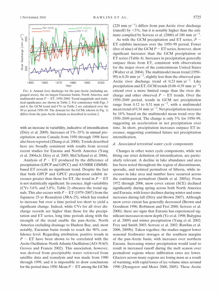
From 1950 through 2004, annual pan-Arctic discharge

exhibits a significant, positive trend of 0.23 mm yr22

(5.3 km3 yr22), significant at the 90% confidence level

(Fig. 6; Table 2). The majority of river flow to the Arctic

Ocean originates from Eurasia, a region with long re-

cords relative to North America. River discharge from

the six largest Eurasian river basins has exhibited a sus-

tained long-term increase over the past 701 yr (Peterson

et al. 2002; Shiklomanov and Lammers 2009). This is

reflected in the greater trend (0.31 mm yr22) for Eurasia

compared to the pan-Arctic trend. In contrast to the

increased flow for Eurasia, no significant change is evi-

dent for the Arctic drainage of North American as a

whole over the same period. However, when the flow

to Hudson Bay is excluded, a large significant increase

(0.40 mm yr22) emerges. In turn, estimates for Hudson

Bay from 1950 through 2005 exhibit no trend. Other

studies have noted significant declines in the flow to

Hudson Bay since 1964 (Dery et al. 2005; McClelland

et al. 2006). More recent data (1989–2007), however, show

a 15.5% increase in the annual flows from Canada along


with an increase in variability, indicative of intensification

(Dery et al. 2009). Increases of 5%–35% in annual pre-

cipitation across Canada from 1950 through 1998 have

also been reported (Zhang et al. 2000). Trends described

here are broadly consistent with results from several

recent studies for Eurasia and North America (Yang

et al. 2004a,b; Dery et al. 2005; McClelland et al. 2006).

Analysis of P 2 ET produced by the difference of

precipitation (GPCP and GPCC) and AVHRR GIMMS-

based ET reveals no significant trend. Despite the fact

that both GPCP and GPCC precipitation exhibit in-

creases greater than those for ET, the trend in P 2 ET

is not statistically significant. In essence, high variability

(CVs 5.6% and 5.8%; Table 2) obscures the trend sig-

nals. This also occurs with P 2 ET (1979–2007) from the

Japanese 25-yr Reanalysis (JRA-25), which has tended

to increase but over a time period too short to yield a

significant change. Indeed, while CVs for all river dis-

charge records are higher than those for the precipi-

tation and ET series, long time periods along with the

strength of the trend enable the pan-Arctic, North

America excluding drainage to Hudson Bay, and, most

notably, Eurasian basin trends to reach the 90% con-

fidence level. Regarding attribution, positive trends in

P 2 ET have been shown to be correlated with the

Arctic Oscillation–North Atlantic Oscillation (AO–NAO;

Groves and Francis 2002). This association, however,

was derived from precipitable water retrieved from

satellite data and reanalysis and was made from 1980

through 1999, and it is impossible to draw conclusions

for the period since 1950. Mean P 2 ET among the GCMs

(220 mm yr21) differs from pan-Arctic river discharge

(runoff) by ,5%, but it is notably higher than the esti-

mate compiled by Serreze et al. (2006) of 180 mm yr21.

As with the GCM precipitation and ET series, P 2

ET exhibits increases over the 1950–99 period. Fewer

(five of nine) of the GCM P 2 ET series, however, show

significant increases than the GCM precipitation or

ET series (Table 4). Increases in precipitation generally

outpace those from ET, consistent with observations

for the major rivers of the conterminous United States

(Walter et al. 2004). The multimodel mean trend (1950–

99) is 0.20 mm yr22, slightly less than the observed pan-

Arctic river discharge trend of 0.23 mm yr22. Like

precipitation and ET, GCM trends (0.06–0.39 mm yr22)

extend over a more limited range than the river dis-

charge and other observed P 2 ET trends. Over the

1950–2049 period, trends in GCM net precipitation

range from 0.12 to 0.51 mm yr22, with a multimodel

mean trend of 0.34 mm yr22. Net precipitation increases

by 18% based on the multimodel mean trend over the

1950–2049 period. The change is only 5% for 1950–99,

suggesting an acceleration in net precipitation over

time. In short, precipitation increases outpace ET in-

creases, suggesting continued future net precipitation

intensification.

d. Associated terrestrial water cycle components

Changes in other water cycle components, while not

fitting our strict definition of intensification, are partic-

ularly relevant. A decline in lake abundance and area

has been noted throughout the region of discontinuous,

sporadic, and isolated permafrost of Siberia, while in-

creases in lake area and number have occurred across

the continuous permafrost (Smith et al. 2005a). From

1972 through 2006, snow cover extent (SCE) declined

significantly during spring across both North America

and Eurasia, with lesser declines during winter and some

increases during fall (Dery and Brown 2007). Although

snow cover extent has generally decreased (Brown and

Goodison 1996; Robinson and Frei 2000; Serreze et al.

2000), there are signs that Eurasia has experienced sig-

nificant increases in snow depth (Ye et al. 1998; Bulygina

et al. 2009) and winter precipitation (Yang et al. 2002;

Frey and Smith 2003; Serreze et al. 2002; Rawlins et al.

2006, 2009b). Taken together, the studies suggest lower

seasonal freshwater storages at the southern margins

of the pan-Arctic basin, with increases over northern

Eurasia. Increasing winter precipitation would tend to

result in increased runoff during the melt season over

permafrost regions where infiltration rates are lower.

Glaciers across many regions are losing mass as a result

of warming, with rapid losses of ice volume since around

1990 (Dyurgerov and Meier 2000, 2005). These Arctic

FIG. 6. Annual river discharge for the pan-Arctic (including un-

gauged areas), the six largest Eurasian basins, North America, and

multimodel mean P 2 ET, 1950–2004. Trend magnitude and statis-

tical significance are shown in Table 2. For consistency with Figs. 3

and 4, the GCM trend and CVs in Table 2 are calculated over the

50-yr period 1950–99. The domain for the GCMs (shown in Fig. 1)

differs from the pan-Arctic domain as described in section 2.


glacier trends are generally consistent with global de-

clines but quantitatively smaller, and the contribution

of glacier melt to river flow across the pan-Arctic is

small. Other major changes include a lengthening of

the growing season, which may be an important com-

ponent in the upward ET trend. Estimates from remote

sensing and CO2 flask measurements suggest an ad-

vance in growing season from 1.5 to 4 days per decade

(McDonald et al. 2004; Zhang et al. 2009).

Observed evidence of changes in active layer thick-

ness (ALT) and permafrost conditions is substantial

worldwide. Permafrost temperatures have increased up

to 38C during the past several decades across parts of

the terrestrial pan-Arctic (Osterkamp 2005; Smith et al.

2005b; Pavlov 1994; Oberman and Mazhitowa 2001).

Changes in air temperature alone cannot account for

the permafrost temperature increase, which suggests

that changes in seasonal snow cover conditions may also

be involved (Zhang and Osterkamp 1993; Zhang 2005).

Based on soil temperature measurements in the active

layer and upper permafrost up to 3.2 m from 37 hydro-

meteorological stations in Russia, the active layer ex-

hibited a statistically significant deepening of about 25 cm

from the early 1960s to 1998 (Frauenfeld et al. 2004;

Zhang et al. 2005). The International Permafrost Asso-

ciation (IPA) started a network of the Circumpolar Ac-

tive Layer Monitoring (CALM) program in the 1990s to

monitor the response of the active layer and upper per-

mafrost to climate change and currently incorporates

more than 125 sites worldwide (Brown et al. 2000). The

results from high-latitude sites in North America dem-

onstrate substantial interannual and interdecadal fluctu-

ations but with no significant trend in ALT in response to

increasing air temperatures. Evidence from the CALM

European monitoring sites suggests that ALT was great-

est in the summers of 2002 and 2003 (Harris et al. 2003).

ALT has increased by up to 1.0 m over the Qinghai–

Tibetan Plateau since the early 1980s (Zhao et al. 2004).

The effect of increasing ALT on the Arctic FWC is

complicated. Freezing of soil moisture reduces the soil

hydraulic conductivity, leading to either more runoff

due to decreased infiltration or higher soil moisture con-

tent due to restricted drainage. The existence of a thin

frozen layer near the surface decouples soil moisture

exchange between the atmosphere and deeper soils

(Zhang et al. 2005; Ye et al. 2009). Permafrost essen-

tially limits the amount of subsurface water storage and

infiltration that can occur, leading to wet soils and ponded

surface waters, unusual for a region with such limited

precipitation. An increase in ALT, on one hand, directly

increases groundwater storage capacity and thus reduces

river discharge through partitioning of surface runoff

from snowmelt and/or rainfall. On the other hand, melting

of excess ground ice near the permafrost surface can

contribute water to runoff and potentially increase river

discharge. In this case, less ice would tend to result in

more moisture available for evaporation and transpira-

tion compared to a thinner ALT and a longer period

of frozen surface soil. Changes in the movement of wa-

ter within the soil column may be occurring. Increases

in thaw depth and, in turn, soil water flowpaths have

been inferred from geochemical tracers in Alaskan

North Slope streams (Keller et al. 2010). Model studies

point to potentially large future increases in river dis-

charge because of permafrost thaw (Lawrence and Slater

2005). The net effect of this change on river discharge

thus requires further study and long-term monitoring.

4. Marine system

a. Freshwater exchanges with the Atlanticand Pacific Oceans

We consider in this section the inflows and outflows of

liquid (ocean) freshwater as well as the solid (sea ice)

component. The inflows occur in the Bering Strait, the

eastern side of Fram Strait, and the Barents Sea (ice only).

Outflows occur through the Canadian Arctic Archipelago,

the western side of Fram Strait, and the Barents Sea

(ocean only). All freshwater fluxes are calculated rel-

ative to a salinity of 34.8, except where noted.

1) FRAM STRAIT ICE FLUX

The mean annual ice concentration–weighted area

outflow at the Fram Strait over the period 1979–2007 has

been computed using satellite data as (706 6 113) 3

103 km2. There is no statistically significant long-term

trend in the Fram Strait area flux in the 29-yr record,

a reflection of an increasing cross-strait sea level pres-

sure gradient (i.e., stronger local winds) and a decreas-

ing ice concentration (Kwok 2009). Turning to volume

flux, the best estimate of the mean annual volume flux

using satellite and mooring data between 1991 and 1999

is ;2200 km3 yr21 [;0.07 Sv (1 Sv [ 106 m3 s21); Kwok

et al. (2004)] , or ;0.3 m of Arctic Ocean sea ice (area of

7.2 million km2). It is not readily apparent from this

short 9-yr record that there is any discernible trend in

annual ice volume exiting the Fram Strait. A recent up-

date by Spreen et al. (2009) also finds no trend.

On average, the IPCC models (Fig. 7) show higher

area outflow and lower ice concentration in the Fram

Strait than observational estimates. However, in agree-

ment with the 29-yr observational record, there is no

trend in the model simulations of area outflow. Even

though the average model behavior does not show a neg-

ative trend in the ice concentration during the period


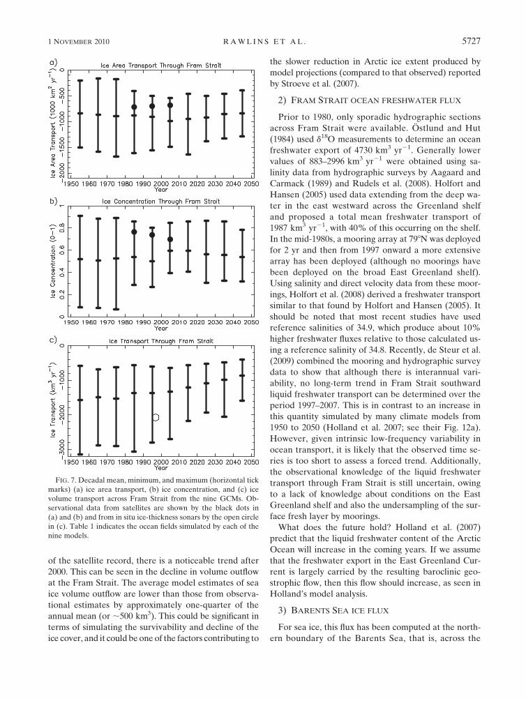
of the satellite record, there is a noticeable trend after

2000. This can be seen in the decline in volume outflow

at the Fram Strait. The average model estimates of sea

ice volume outflow are lower than those from observa-

tional estimates by approximately one-quarter of the

annual mean (or ;500 km3). This could be significant in

terms of simulating the survivability and decline of the

ice cover, and it could be one of the factors contributing to

the slower reduction in Arctic ice extent produced by

model projections (compared to that observed) reported

by Stroeve et al. (2007).

2) FRAM STRAIT OCEAN FRESHWATER FLUX

Prior to 1980, only sporadic hydrographic sections

across Fram Strait were available. Ostlund and Hut

(1984) used d18O measurements to determine an ocean

freshwater export of 4730 km3 yr21. Generally lower

values of 883–2996 km3 yr21 were obtained using sa-

linity data from hydrographic surveys by Aagaard and

Carmack (1989) and Rudels et al. (2008). Holfort and

Hansen (2005) used data extending from the deep wa-

ter in the east westward across the Greenland shelf

and proposed a total mean freshwater transport of

1987 km3 yr21, with 40% of this occurring on the shelf.

In the mid-1980s, a mooring array at 798N was deployed

for 2 yr and then from 1997 onward a more extensive

array has been deployed (although no moorings have

been deployed on the broad East Greenland shelf).

Using salinity and direct velocity data from these moor-

ings, Holfort et al. (2008) derived a freshwater transport

similar to that found by Holfort and Hansen (2005). It

should be noted that most recent studies have used

reference salinities of 34.9, which produce about 10%

higher freshwater fluxes relative to those calculated us-

ing a reference salinity of 34.8. Recently, de Steur et al.

(2009) combined the mooring and hydrographic survey

data to show that although there is interannual vari-

ability, no long-term trend in Fram Strait southward

liquid freshwater transport can be determined over the

period 1997–2007. This is in contrast to an increase in

this quantity simulated by many climate models from

1950 to 2050 (Holland et al. 2007; see their Fig. 12a).

However, given intrinsic low-frequency variability in

ocean transport, it is likely that the observed time se-

ries is too short to assess a forced trend. Additionally,

the observational knowledge of the liquid freshwater

transport through Fram Strait is still uncertain, owing

to a lack of knowledge about conditions on the East

Greenland shelf and also the undersampling of the sur-

face fresh layer by moorings.

What does the future hold? Holland et al. (2007)

predict that the liquid freshwater content of the Arctic

Ocean will increase in the coming years. If we assume

that the freshwater export in the East Greenland Cur-

rent is largely carried by the resulting baroclinic geo-

strophic flow, then this flow should increase, as seen in

Holland’s model analysis.

3) BARENTS SEA ICE FLUX

For sea ice, this flux has been computed at the north-

ern boundary of the Barents Sea, that is, across the

FIG. 7. Decadal mean, minimum, and maximum (horizontal tick

marks) (a) ice area transport, (b) ice concentration, and (c) ice

volume transport across Fram Strait from the nine GCMs. Ob-

servational data from satellites are shown by the black dots in

(a) and (b) and from in situ ice-thickness sonars by the open circle

in (c). Table 1 indicates the ocean fields simulated by each of the

nine models.


passages between Svalbard and Franz Josef Land (S-FJL)

and between Franz Josef Land and Severnaya Zemlya

(FJL-SZ). In the 29-yr record of ice area flux from sat-

ellite estimates (Kwok 2009), there is a mean annual

inflow to the Arctic Ocean of seasonal ice through the

FJL-SZ passage of (103 6 93) 3 103 km2. The source of

this sea ice is the Barents Sea as well as the Kara Sea.

The annual outflow at the S-FJL passage is (37 6 39) 3

103 km2—that is, ;5% of the Fram Strait area export,

with no statistically significant trend. The result is a net

inflow of sea ice to the Arctic Ocean of 66 3 103 km2,

with no trend. Thus, the Barents Sea is a net producer

of sea ice, which is exported northward to the Arctic

Ocean. This ice presumably is swept into the sea ice

circulation that exits the Arctic Ocean via Fram Strait.

4) BARENTS SEA OCEAN FRESHWATER FLUX

The oceanic freshwater flux has been monitored at

the western boundary of the Barents Sea across longi-

tude 208E. The fluxes are composed of contributions

from the relatively fresh eastward-flowing Norwegian

Coastal Current (NCC), the relatively saline Atlantic in-

flow with the North Cape Current (NCaC), and the out-

flowing recirculated Atlantic water in the Bear Island

Trough (BIT) (Bjork et al. 2001; Skagseth et al. 2008).

The hydrographic variations of these branches have been

monitored somewhat sporadically since the 1960s and

regularly since 1977 (4–6 times per year). Since 1997,

these measurements have been complemented with an

array of current-meter moorings. For the NCaC and the

BIT outflow, the annual mean volume fluxes are com-

bined with the observed deseasoned long-term core sa-

linities to obtain the freshwater fluxes. The freshwater

flux in the NCC is estimated based on vertical profiles

by assuming geostrophic balance, with a zero velocity

reference assumed at a density outcrop (Orvik et al.

2001). The baroclinic transport is then combined with

vertical profiles of salinity to get the freshwater flux.

The total and individual contributions to the fresh-

water are summarized in Table 5. In total, there is a

freshwater outflow of 84 km3 yr21, which is the sum of

a large NCaC outflow (i.e., inflowing water saltier than

the reference salinity) and two smaller inflows from

the NCC and from the Bear Island Trough recircula-

tion. There is a long-term decrease in the total outflow

from 115 km3 yr21 for the period 1965–84 compared

to 55 km3 yr21 for the period 1985–2005. This is due

to an increased NCC freshwater inflow associated

with increased precipitation over northern Europe and

Scandinavia.

An anticipated future warming and more atmospheric

moisture content will probably act to continue the fresh-

ening of the NCC. On the other hand, the freshwater

fluxes associated with the NCaC and the Bear Island

Trough recirculation are dependent on the local regional

wind forcing (Ingvaldsen et al. 2002) as well the salinity

of the Atlantic water. Future trends in these variables

are very uncertain.

5) BERING STRAIT ICE FLUX

Initial work (Aagaard and Carmack 1989) estimated

the Bering Strait freshwater flux from ice as an inflow to

the Arctic Ocean of 24 km3 yr21. The present best ob-

servational estimate is an inflow of 100 6 70 km3 yr21,

assuming a sea ice salinity of 7 psu (Woodgate and

Aagaard 2005), although this is highly speculative, being

based on the extrapolation of data of ice thickness and

ice motion from one mooring in the center of the strait.

No long-term trends have been computed. Comparison

of modeled ice freshwater fluxes (not shown) shows a

greater spread than the oceanic freshwater flux (next

section). In particular, the three models that simulate

the most realistic Bering Strait ocean freshwater flux

differ in sign for the ice freshwater flux.

6) BERING STRAIT OCEAN FRESHWATER FLUX

A 14-yr (1990–2004) dataset of year-round near-

bottom measurements in the Bering Strait was com-

bined by Woodgate and Aagaard (2005) with estimates

of sea ice flux and freshwater transport within the Alas-

kan Coastal Current (ACC) and in the summer stratified

surface layer to yield a 14-yr mean ocean freshwater

transport of 2500 6 300 km3 yr21. Interannual variabil-

ity in the observational estimates is substantial. Without

considering the contributions from the ACC or stratifi-

cation [likely adding ;(800–1000) km3 yr21], annual

mean freshwater transport through the Bering Strait is

estimated to vary between ;1400 and 2000 km3 yr21,

with lows in the early 2000s (Woodgate et al. 2006). It is

noteworthy that the freshwater increase between 2001

and 2004 is ;800 km3, about one-quarter of annual Arctic

river runoff. About 80% of the increase in freshwater can

TABLE 5. Freshwater fluxes (relative to a salinity of 34.8) across

208E in the two inflowing currents (Norwegian Coastal Current and

North Cape Current) and the outflowing recirculation in the Bear

Island Trough. Positive values indicate freshwater inflow to the

Barents Sea.

Freshwater flux (km3 yr21)

Mean

1965–2005

Mean

1965–84

Mean

1985–2005

Norwestern Coastal Current 246 197 294

North Cape Current 2502 2484 2519

Bear Island Trough 172 173 170

Total 284 2115 255


be accounted for by the increased volume flux over the

same time period, which in turn may be related to changes

in the local wind.

Coupled model simulations of the oceanic Bering

Strait freshwater flux vary widely (not shown). How-

ever, the multimodel ensemble mean produces a long-

term mean value close to observations, also reproduced

by the Canadian Centre for Climate Modelling and Anal-

ysis (CCCma) Coupled General Circulation Model, ver-

sion 3.1 (CGCM3.1), the Model for Interdisciplinary

Research on Climate 3.2 (MIROC3.2), and CCSM3 indi-

vidual runs. Modeled long-term trends are small (Holland

et al. 2007; their Fig. 8), with changes of ;200 km3 yr21

over a 100-yr period. This change is generally smaller

than the observed interannual variability over 1990–2004.

7) CANADIAN ARCHIPELAGO ICE FLUX

Over the period between 1997 and 2002, high-resolution

radar imagery in the western archipelago (Kwok 2006)

has been used to estimate mean annual sea ice areal

fluxes through the Amundsen Gulf, M’Clure Strait, and

the Queen Elizabeth Islands of (85 6 26) 3 103, (20 6

24) 3 103, and 2(8 6 6) 3 103 km2 (negative sign in-

dicates outflow). Overall, sea ice is imported from the

Canadian Archipelago into the Arctic Ocean in this

area, providing a volume inflow of roughly 100 km3 yr21.

This is balanced by the export of Arctic Ocean sea

ice through Nares Strait in the northeastern archi-

pelago. Kwok et al. (2005) computed an average an-

nual (September–August) ice area outflow of 33 km3

across the 30-km-wide northern entrance at Robeson

Channel. Thick, multiyear ice coverage in Nares Strait

is high (.80%), with volume outflow estimated to be

;100 km3 yr21—that is, ;5% of the mean annual Fram

Strait ice flux and exactly opposite to the inflow calcu-

lated for the western archipelago. However, it is im-

portant to note that these short time series may not be

representative of the long-term balance, and they have

not yet been used to calculate long-term trends. An in-

teresting recent phenomenon is the failure of winter ice

arches to form within Nares Strait, which if this con-

tinues would sustain the export of very thick ice from the

Arctic Ocean.

8) CANADIAN ARCHIPELAGO OCEAN

FRESHWATER FLUX

Total ocean freshwater transport through the various

straits of the Archipelago has been estimated using his-

torical data as roughly (900–4000) 6 1000 km3 yr21

(Aagaard and Carmack 1989; Tang et al. 2004; Cuny

et al. 2005; Dickson et al. 2007; Serreze et al. 2006), with

more recent efforts placing tighter constraints on fluxes

through the major passages of Nares Strait (Munchow

et al. 2006) and Lancaster Sound (Prinsenberg and

Hamilton 2005). An attractive option is to measure the

flux across Davis Strait to the south, which theoretically

should integrate all of these fluxes. Recent analysis of

mooring data taken since 2004 (unpublished) indicates

a decline in net southward freshwater flux, but this is

not statistically significant. Most models analyzed by

Holland et al. (2007) did not include an open Canadian

Archipelago. However, the CCSM model analyzed by

Holland et al. (2006) did provide flux estimates through

this area. The model results (not shown) estimate fresh-

water fluxes of about 1388 km3 yr21 over the twentieth

century, which is within the historical range.

9) NET PRECIPITATION

The P 2 ET over the Arctic Ocean for the period

1979–2007, estimated from the atmospheric moisture

budget (wind and vapor flux fields) of JRA-25, shows

no trend. And while annual P 2 ET derived from pre-

cipitable water retrieved from the Television and Infra-

red Observation Satellite (TIROS) Operational Vertical

Sounder (TOVS) and upper-level winds from the NCEP–

NCAR reanalysis suggest recent increases in Arctic

Ocean net precipitation (1989–98 average versus 1980–88

average), the decadal difference is small (4.2% of the

19-yr mean) and not statistically significant (Groves and

Francis 2002).

b. Freshwater storage within the Arctic Ocean

1) SEA ICE

Rothrock et al. (2008) showed that over the period

1975–2000, annual mean Arctic Ocean sea ice thick-

ness decreased by 1.25 m (i.e., ;31%), with the maxi-

mum thickness in 1980 and the minimum in 2000. The

sharpest rate of decline occurred in 1990, with a much

slower rate by the end of the record. More recently,

Giles et al. (2008) analyzed satellite-based radar altim-

eter data that indicate relatively constant ice thickness

between 2003 and 2007, followed by a substantial de-

crease between 2007 and 2008.

The decline in ice freshwater storage is due to a com-

bination of a loss of ice thickness and a loss of ice area.

The estimated loss in thickness is on the order of 30%

from 1975 to 2000 (Rothrock et al. 2008). Comiso and

Nishio (2008) used passive microwave satellite data over

1979–2006 to estimate ice area loss as 2% per decade in

winter and 9% in summer. Over the period from 1975

to 2000 the total loss in ice freshwater storage would

therefore be on the order of 40%. None of the coupled

GCMs shown in Fig. 8 comes close to this. The largest

decline over this period is around 25% in the CCSM3

and MIROC3.2 model runs. The average of all the


models is nearly half that or a decline of only around

13%. One potential caveat is that the submarine ice

thickness data come only from the central basin, whereas

the model includes seasonal areas that may have experi-

enced a lesser decline.

It is likely that we will see a continuing decline of

freshwater storage in the ice. The lengthening melt sea-

son will result in continued thinning of the ice and a

steady decrease in ice extent. Further, the ice is prone

to episodic wind events, such as the Arctic Oscillation

shift around 1990 that flushed old, thick ice out of the

Arctic Ocean. The thinning of the ice has led many to

refer to the ice pack as ‘‘vulnerable’’ both to steady

warming and episodic events.

2) OCEAN

Steele and Ermold (2004), Swift et al. (2005),

Dmitrenko et al. (2008), and Polyakov et al. (2008) find

that between the late 1960s–1970s and the late 1990s,

freshwater declined in the central Arctic Ocean, whereas

it increased (but to a much lesser extent) on the Russian

arctic shelves to the west of the East Siberian Sea. The

central Arctic decline was ;1500 km3, composed of

relatively long periods (;15 yr) of increasing values,

alternating with shorter (;5 yr) periods of decline.

This behavior was described as a ‘‘freshwater capaci-

tor’’ by Proshutinsky et al. (2002), referring to the buildup

of freshwater within the Beaufort Gyre and its sub-

sequent release to the North Atlantic Ocean over a rela-

tively shorter period. An example from the late 1980s to

early 1990s was simulated in an ice–ocean model study by

Karcher et al. (2005). This alternating increase–decrease

in ocean freshwater has been linked to wind forcing as-

sociated with the Arctic Oscillation, although other fac-

tors may also play a role. In recent years (since 2000), this

index has declined, which suggests a collection of fresh-

water in the Beaufort Gyre as noted by McPhee et al.

(2009).

Figure 9 extends the results of Holland et al. (2007) by

showing detailed ocean freshwater time series from the

available IPCC CMIP3 models. Over the latter half of

the twentieth century, most models show a relatively

weak freshwater increase, which for the multimodel

mean amounts to about 3000 km3. This is of the opposite

sign and double the value of the observed freshwater

decrease over this time period. Why is this? The ob-

served changes in freshwater storage respond to wind

forcing associated with low-frequency variations in the

Arctic Oscillation (Steele and Ermold 2007; Polyakov

et al. 2008). These variations acted to collect freshwater

(sea ice plus ocean freshwater) in the Arctic Ocean be-

fore the 1960s and then to force it southward into the

North Atlantic Ocean through the rest of the century.

It is likely that some component of this time evolution

was the result of intrinsic climate variability, the ob-

served phase that climate models are not expected to

capture, even with ensemble runs. Climate models gen-

erally simulate much weaker trends in the Arctic Os-

cillation over the late twentieth century than observed

(Gillett et al. 2002; Teng et al. 2006). However, it is un-

clear whether this discrepancy arises from a deficiency

in the models’ simulated response to anthropogenic

forcing or the fact that some Arctic Oscillation anom-

alies represent extremely large variations in the real

climate system.

c. Summary of marine freshwater changes

Table 6 summarizes the observed trends in sea ice and

ocean freshwater fluxes and storage, as determined from

the information in previous sections. We note no trend

FIG. 8. Freshwater storage in sea ice, 1950–2049. The heavy black

line is the multimodel mean.FIG. 9. Liquid freshwater storage, 1950–2049. The heavy black line

is the multimodel mean.


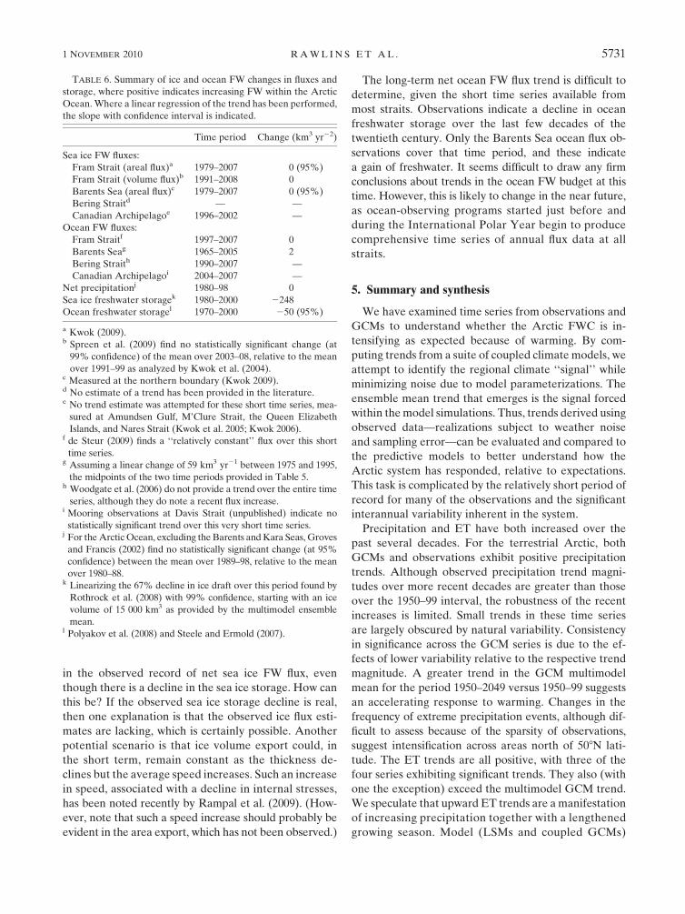
in the observed record of net sea ice FW flux, even

though there is a decline in the sea ice storage. How can

this be? If the observed sea ice storage decline is real,

then one explanation is that the observed ice flux esti-

mates are lacking, which is certainly possible. Another

potential scenario is that ice volume export could, in

the short term, remain constant as the thickness de-

clines but the average speed increases. Such an increase

in speed, associated with a decline in internal stresses,

has been noted recently by Rampal et al. (2009). (How-

ever, note that such a speed increase should probably be

evident in the area export, which has not been observed.)

The long-term net ocean FW flux trend is difficult to

determine, given the short time series available from

most straits. Observations indicate a decline in ocean

freshwater storage over the last few decades of the

twentieth century. Only the Barents Sea ocean flux ob-

servations cover that time period, and these indicate

a gain of freshwater. It seems difficult to draw any firm

conclusions about trends in the ocean FW budget at this

time. However, this is likely to change in the near future,

as ocean-observing programs started just before and

during the International Polar Year begin to produce

comprehensive time series of annual flux data at all

straits.

5. Summary and synthesis

We have examined time series from observations and

GCMs to understand whether the Arctic FWC is in-

tensifying as expected because of warming. By com-

puting trends from a suite of coupled climate models, we

attempt to identify the regional climate ‘‘signal’’ while

minimizing noise due to model parameterizations. The

ensemble mean trend that emerges is the signal forced

within the model simulations. Thus, trends derived using

observed data—realizations subject to weather noise

and sampling error—can be evaluated and compared to

the predictive models to better understand how the

Arctic system has responded, relative to expectations.

This task is complicated by the relatively short period of

record for many of the observations and the significant

interannual variability inherent in the system.

Precipitation and ET have both increased over the

past several decades. For the terrestrial Arctic, both

GCMs and observations exhibit positive precipitation

trends. Although observed precipitation trend magni-

tudes over more recent decades are greater than those

over the 1950–99 interval, the robustness of the recent

increases is limited. Small trends in these time series

are largely obscured by natural variability. Consistency

in significance across the GCM series is due to the ef-

fects of lower variability relative to the respective trend

magnitude. A greater trend in the GCM multimodel

mean for the period 1950–2049 versus 1950–99 suggests

an accelerating response to warming. Changes in the

frequency of extreme precipitation events, although dif-

ficult to assess because of the sparsity of observations,

suggest intensification across areas north of 508N lati-

tude. The ET trends are all positive, with three of the

four series exhibiting significant trends. They also (with

one the exception) exceed the multimodel GCM trend.

We speculate that upward ET trends are a manifestation

of increasing precipitation together with a lengthened

growing season. Model (LSMs and coupled GCMs)

TABLE 6. Summary of ice and ocean FW changes in fluxes and

storage, where positive indicates increasing FW within the Arctic

Ocean. Where a linear regression of the trend has been performed,

the slope with confidence interval is indicated.

Time period Change (km3 yr22)

Sea ice FW fluxes:

Fram Strait (areal flux)a 1979–2007 0 (95%)

Fram Strait (volume flux)b 1991–2008 0

Barents Sea (areal flux)c 1979–2007 0 (95%)

Bering Straitd — —

Canadian Archipelagoe 1996–2002 —

Ocean FW fluxes:

Fram Straitf 1997–2007 0

Barents Seag 1965–2005 2

Bering Straith 1990–2007 —

Canadian Archipelagoi 2004–2007 —

Net precipitationj 1980–98 0

Sea ice freshwater storagek 1980–2000 2248

Ocean freshwater storagel 1970–2000 250 (95%)

a Kwok (2009).b Spreen et al. (2009) find no statistically significant change (at

99% confidence) of the mean over 2003–08, relative to the mean

over 1991–99 as analyzed by Kwok et al. (2004).c Measured at the northern boundary (Kwok 2009).d No estimate of a trend has been provided in the literature.e No trend estimate was attempted for these short time series, mea-

sured at Amundsen Gulf, M’Clure Strait, the Queen Elizabeth

Islands, and Nares Strait (Kwok et al. 2005; Kwok 2006).f de Steur (2009) finds a ‘‘relatively constant’’ flux over this short

time series.g Assuming a linear change of 59 km3 yr21 between 1975 and 1995,

the midpoints of the two time periods provided in Table 5.h Woodgate et al. (2006) do not provide a trend over the entire time

series, although they do note a recent flux increase.i Mooring observations at Davis Strait (unpublished) indicate no

statistically significant trend over this very short time series.j For the Arctic Ocean, excluding the Barents and Kara Seas, Groves

and Francis (2002) find no statistically significant change (at 95%

confidence) between the mean over 1989–98, relative to the mean

over 1980–88.k Linearizing the 67% decline in ice draft over this period found by

Rothrock et al. (2008) with 99% confidence, starting with an ice

volume of 15 000 km3 as provided by the multimodel ensemble

mean.l Polyakov et al. (2008) and Steele and Ermold (2007).


analysis of the factors controlling ET fluxes are needed to

resolve differences in the trend magnitudes and linkage

to other water cycle components.

Pan-Arctic river discharge, including discharge from

ungauged regions, has also risen over recent decades.

Among all components, the long-term increase in river

discharge from large Eurasian rivers is perhaps the most

consistent trend evidencing Arctic FWC intensification.

The trend in the combined flow of the six largest Eur-

asian rivers over the period 1936–99 is approximately

7% (Peterson et al. 2002) and is consistent with models

linking net precipitation increases to anthropogenic

forcing (Wu et al. 2005). While discharge increases from

Eurasia dominate the pan-Arctic trend, recent positive

trends from Canada suggest that riverine intensification

may now be pan-Arctic in extent. The time series of pan-

Arctic (including ungauged regions) annual discharge

exhibits a trend that is nearly double the multimodel

mean GCM P 2 ET trend. What might explain why the

trend in observed river discharge exceeds the trend in

net precipitation simulated by the models? One poten-

tial explanation involves recent reported increases in

winter precipitation, which we speculate may not be

adequately captured by the GCMs. There is evidence

that the discharge–precipitation ratio has increased

across Eurasia over the latter decades of the twentieth

century. In other words, more of the increasing precip-

itation flux may now become discharge each year. This

change would be one way for the discharge increases to

keep pace with precipitation increases. Changes in stor-

age may also be involved. Drainage from water bodies

(lakes and ponds) and thawing permafrost are two addi-

tional freshwater sources that could directly contribute to

increases in river discharge and ET. These contributions

would represent water cycle changes not directly linked

with intensification as expressed through physics involv-

ing the Clausius–Clapeyron relation.

River discharge from Eurasia strongly influences fresh-

water budgets along the Russian shelves, which fresh-

ened in recent decades. Ocean circulation, however, plays

a dominant role in this region and largely drives the

freshwater balance (Steele and Ermold 2004). Regard-

ing trends in Arctic Ocean fluxes and stocks, Arctic Os-

cillation trends created a freshwater buildup (ice and

ocean) through the 1960s and then a release of this

freshwater through the rest of the century. This effect

dominated the slow increase in freshwater inflows from

rivers and other sources. What will happen in the future?

It seems likely that wind forcing will continue to play an

important role, sequestering and then releasing both

ocean and ice freshwater over multiyear time scales.

However, over the longer term, increasing freshwater

inputs from river discharge, from ocean advection, and

from net precipitation may eventually come to dominate

the budget and lead to an increasing Arctic Ocean

freshwater content, although this is uncertain.

Simulations with coupled GCMs suggest an intensi-

fication of the Arctic FWC in response to rising green-

house gas concentrations. Observations also suggest

intensification across the terrestrial system. That being

said, our confidence in these change signals, with the

exception of Eurasian river discharge, is somewhat lim-

ited. The lack of strongly significant trends in some of

the observations is reflective of the considerable variabil-

ity in Arctic freshwater system and the sparse/incomplete

measures of precipitation, ET, and river discharge. Inten-

sification of oceanic freshwater fluxes cannot be ascer-

tained given the short records. Additional GCM runs

have been made available to the community during the

completion of this analysis, and new model runs are being

currently produced as part of the IPCC Fifth Assessment

Report. Direct observations of the Arctic FWC are con-

tinually being updated and made available as well. Fu-

ture analysis to update the assessments presented here

will be an important contribution to the emerging body

of evidence documenting Arctic hydrologic change. Con-

tinued positive trends over coming years will need to

occur to increase our confidence that the Arctic FWC is

intensifying as expected because of climatic warming.

Acknowledgments. We acknowledge the modeling

groups, the Program for Climate Model Diagnosis and

Intercomparison (PCMDI) and the WCRP’s Working

Group on Coupled Modeling (WGCM) for their roles in

making available the WCRP CMIP3 multimodel data-

set. Support of this dataset is provided by the Office

of Science, U.S. Department of Energy. We gratefully

acknowledge funding from the National Science Foun-

dation’s Office of Polar Programs through the Fresh-

water Integration Project and from NASA’s Cryosphere

Program. Funding was provided through NSF Grants

ARC-0531040, ARC-0531302, ARC-0612062, ARC-

0629471, ARC-0632154, ARC-0632231, ARC-0633885,

ARC-0652838, ARC-0805789, OPP-0229705, OPP-

0230083, OPP-0230211, OPP-0230381, OPP-0328686,

OPP-0335941, and OPP-0352754 and NASA Grants

NNG06GE43G, NNH04AA66I, NNH08AI57I, and

NNX08AN58G. The lead author was supported by fel-

lowships from the NASA Postdoctoral Program and the

New Hampshire Space Grant Consortium. Portions of

this work were carried out at the Jet Propulsion Labora-

tory, California Institute of Technology, under contract

with the National Aeronautics and Space Administration.

Any use of trade, product, or firm names in this publica-

tion is for descriptive purposes only and does not imply

endorsement by the U.S. Government.


REFERENCES

Aagaard, K., and E. C. Carmack, 1989: The role of sea ice and other

fresh waters in the Arctic circulation. J. Geophys. Res., 94,

14 485–14 498.

Adam, J. C., I. Haddeland, F. Su, and D. P. Lettenmaier, 2007:

Simulation of reservoir influences on annual and seasonal

streamflow changes for the Lena, Yenisei, and Ob rivers.

J. Geophys. Res., 112, D24114, doi:10.1029/2007JD008525.

Alexander, L. V., and Coauthors, 2006: Global observed changes

in daily climate extremes of temperature and precipitation.


Allen, M. R., and W. J. Ingram, 2002: Constraints on future changes

in climate and the hydrologic cycle. Nature, 419, 224–232.

Berbery, E. G., and V. R. Barros, 2002: The hydrologic cycle of the

La Plata Basin in South America. J. Hydrometeor., 3, 630–645.

Berner, J., and Coauthors, Eds., 2005: Arctic Climate Impact As-

sessment. Cambridge University Press, 1042 pp.

Betts, A. K., J. H. Ball, and P. Viterbo, 2003: Evaluation of the

ERA-40 surface water budget and surface temperature for the

Mackenzie River basin. J. Hydrometeor., 4, 1194–1211.

Bjork, G., B. G. Gustafsson, and A. Stigebrandt, 2001: Upper layer

circulation in the Nordic Seas as inferred from the spatial

distribution of heat and freshwater content and potential en-

ergy. Polar Res., 20, 161–168.

Bogdanova, E. G., B. M. Ilyin, and I. V. Dragomilova, 2002: Ap-

plication of a comprehensive bias-correction model to pre-

cipitation measured at Russian North Pole drifting stations.

J. Hydrometeor., 3, 700–713.

Bradley, R. S., H. F. Diaz, J. K. Eischeid, P. D. Jones, P. M. Kelly,

and C. M. Goodess, 1987: Precipitation fluctuations over

Northern Hemisphere land areas since the mid 19th century.

Science, 237, 171–175.

Bromwich, D. H., and R. L. Fogt, 2004: Strong trends in the skill

of the ERA-40 and NCEP–NCAR reanalyses in the high

and middle latitudes of the Southern Hemisphere, 1958–2001.

J. Climate, 17, 4603–4619.

Brown, J., K. M. Hinkel, and F. E. Nelson, 2000: The Circumpolar

Active Layer Monitoring (CALM) program. Polar Geogr., 24,

165–258.

Brown, R. D., and B. E. Goodison, 1996: Interannual variability in

reconstructed Canadian snow cover, 1915–1992. J. Climate, 9,

1299–1318.

Bulygina, O. N., V. N. Razuvaev, and N. N. Korshunova, 2009:

Changes in snow cover over Northern Eurasia in the last few

decades. Environ. Res. Lett., 4, 045026, doi:10.1088/1748-9326/

4/4/045026.

Cherkauer, K. A., L. C. Bowling, and D. P. Lettenmaier, 2003:

Variable infiltration capacity cold land process model updates.

Global Planet. Change, 38, 151–159.

Climatic Research Unit, cited 2009: CRU TS3.0 dataset. [Available

online at http://badc.nerc.ac.uk/data/cru/.]

Comiso, J. C., and F. Nishio, 2008: Trends in the sea ice cover using

enhanced and compatible AMSR-E, SSM/I, and SMMR data.

J. Geophys. Res., 113, C02S07, doi:10.1029/2007JC004257.

Cuny, J., P. B. Rhines, and R. Kwok, 2005: Davis Strait volume,

freshwater and heat fluxes. Deep-Sea Res. I, 52, 519–542.

Curry, R., B. Dickson, and I. Yashayaev, 2003: A change in the

freshwater balance of the Atlantic Ocean over the past four

decades. Nature, 426, 826–829.

Dai, A., T. Qian, K. E. Trenberth, and J. D. Milliman, 2009:

Changes in continental freshwater discharge from 1948 to

2004. J. Climate, 22, 2773–2791.

Dery, S. J., and R. D. Brown, 2007: Recent Northern Hemi-

sphere snow cover extent trends and implications for the snow-

albedo feedback. Geophys. Res. Lett., 34, L22504, doi:10.1029/

2007GL031474.

——, J. Sheffield, and E. F. Wood, 2005: Connectivity between

Eurasian snow cover extent and Canadian snow water equiv-

alent and river discharge. J. Geophys. Res., 110, D23106,

doi:10.1029/2005JD006173.

——, M. A. Hernandez-Henrıquez, J. E. Burford, and E. F. Wood,

2009: Observational evidence of an intensifying hydrological

cycle in northern Canada. Geophys. Res. Lett., 36, L13402,

doi:10.1029/2009GL038852.

de Steur, L., L. E. Hansen, R. Gerdes, M. Karcher, E. Fahrbach,

and J. Holfort, 2009: Freshwater fluxes in the East Greenland

Current: A decade of observations. Geophys. Res. Lett., 36,

L23611, doi:10.1029/2009GL041278.

Dickson, B., I. Yashayaev, J. Meincke, B. Turrell, S. Dye, and

J. Holfort, 2002: Rapid freshening of the deep North Atlantic

Ocean over the past four decades. Nature, 416, 832–836.

Dickson, R., B. Rudels, S. Dye, M. Karcher, J. Meincke, and

I. Yashayaev, 2007: Current estimates of freshwater flux

through Arctic and subarctic seas. Prog. Oceanogr., 73,

210–230.

Dirmeyer, P. A., and K. L. Brubaker, 2007: Characterization of the

global hydrologic cycle from a back-trajectory analysis of at-

mospheric water vapor. J. Hydrometeor., 8, 20–37.

Dmitrenko, I. A., S. A. Kirillov, L. B. Tremblay, D. Bauch, and

M. Makhotin, 2008: The long-term and interannual variability

of summer fresh water storage over the eastern Siberian shelf:

Implication for climatic change. J. Geophys. Res., 113, C03007,

doi:10.1029/2007JC004304.

Dyurgerov, M., and M. Meier, 2000: Twentieth century climate

change: Evidence from small glaciers. Proc. Natl. Acad. Sci.

USA, 97, 1406–1411.

——, and ——, 2005: Year-to-year fluctuations of global mass

balance of small glaciers and their contribution to sea-level

changes. Arct. Antarct. Alp. Res., 29, 392–402.

European Centre for Medium-Range Weather Forecasts, 2002:

ERA-40 Project Report Series. 3. Workshop on Re-analysis,

5–9 November 2001. ECMWF Tech. Rep., 443 pp.

Fernandes, R., V. Korolevych, and S. Wang, 2007: Trends in land

evapotranspiration over Canada for the period 1960–2000

based on in situ climate observations and a land surface model.

J. Hydrometeor., 8, 1016–1030.

Finnis, J., J. J. Cassano, M. Holland, M. C. Serreze, and P. Uotila,

2009: Synoptically forced hydroclimatology of major Arctic

watersheds in general circulation models. Part 2: Eurasian

watersheds. Int. J. Climatol., 29, 1244–1261.

Førland, E. J., and I. Hanssen-Bauer, 2000: Increased precipitation

in the Norwegian Arctic: True or false? Climatic Change, 46,

485–509.

Francis, J. A., J. J. Cassano, W. J. Gutowski Jr., L. D. Hinzman,

M. M. Holland, M. A. Steele, D. M. White, and C. J. Vorosmarty,

2009: An Arctic hydrologic system in transition: Feedbacks

and impacts on terrestrial, marine, and human life. J. Geo-

phys. Res., 114, G04019, doi:10.1029/2008JG000902.

Frauenfeld, O., T. Zhang, R. G. Barry, and D. G. Gilichinsky,

2004: Interdecadal changes in seasonal freeze and thaw

depths in Russia. J. Geophys. Res., 109, D05101, doi:10.1029/

2003JD004245.

Frey, K. E., and L. C. Smith, 2003: Recent temperature and pre-

cipitation increases in West Siberia and their association with

the Arctic Oscillation. Polar Res., 22, 287–300.


Frich, P., L. V. Alexander, P. Della-Marta, B. Gleason, M. Haylock,

A. M. G. Klein-Tank, and T. C. Peterson, 2002: Observed co-

herent changes in climatic extremes during the second half of

the twentieth century. Climate Res., 19, 193–212.

Gaffen, D. J., and R. J. Ross, 1998: Increased summertime heat

stress in the US. Nature, 396, 529–530.

Giles, K. A., S. W. Laxon, and A. L. Ridout, 2008: Circumpolar

thinning of Arctic sea ice following the 2007 record ice ex-

tent minimum. Geophys. Res. Lett., 35, L22502, doi:10.1029/

2008GL035710.

Gillett, N., M. Allen, R. McDonald, C. Senior, D. Shindell, and

G. Schmidt, 2002: How linear is the Arctic Oscillation re-

sponse to greenhouse gases? J. Geophys. Res., 107, 4022,

doi:10.1029/2001JD000589.

Goodison, B. E., P. Y. T. Louie, and D. Yang, 1998: WMO solid

precipitation measurement intercomparison. World Meteo-

rological Organization Rep. WMO/TD 872, 212 pp.

Gorodetskaya, I. V., L. B. Tremblay, B. Liepert, M. A. Cane, and

R. I. Cullather, 2008: The influence of cloud and surface

properties on the Arctic Ocean shortwave radiation budget in

coupled models. J. Climate, 21, 866–882.

Groisman, P. Ya., V. V. Koknaeva, T. A. Belokrylova, and T. R. Karl,

1991: Overcoming biases of precipitation measurement: A

history of the USSR experience. Bull. Amer. Meteor. Soc.,

72, 1725–1733.

——, and Coauthors, 2003: Contemporary climate changes in high

latitudes of the Northern Hemisphere: Daily time resolution.

Proc. 14th Symp. on Global Change and Climate Variations,

Long Beach, CA, Amer. Meteor. Soc., 4.8. [Available online

at http://ams.confex.com/ams/annual2003/techprogram/paper_

54814.htm.]

——, R. W. Knight, D. R. Easterling, T. R. Karl, G. C. Hegerl, and

V. N. Razuvaev, 2005: Trends in intense precipitation in the

climate record. J. Climate, 18, 1326–1350.

——, and Coauthors, 2007: Potential forest fire danger over

Northern Eurasia: Changes during the 20th century. Global

Planet. Change, 56, 371–386.

Groves, D. G., and J. A. Francis, 2002: Variability of the Arctic

atmospheric moisture budget from TOVS satellite data. J. Geo-

phys. Res., 107, 4785, doi:10.1029/2002JD002285.

Hanssen-Bauer, I., and E. J. Forland, 1994: Homogenizing of long

Norweigian precipitation series. J. Climate, 7, 1001–1013.

Harris, C., and Coauthors, 2003: Warming permafrost in European

mountains. Global Planet. Change, 39, 215–225.

Held, I. M., and B. J. Soden, 2006: Robust responses of the hy-

drological cycle to global warming. J. Climate, 19, 5686–5699.

Holfort, J., and E. Hansen, 2005: Timeseries of polar water proper-

ties in Fram Strait. Geophys. Res. Lett., 32, L19601, doi:10.1029/

2005GL022957.

——, ——, S. Østerhus, S. Dye, S. Jonsson, J. Meincke,

J. Mortensen, and M. Meredith, 2008: Freshwater fluxes east

of Greenland. Arctic-Subarctic Ocean Fluxes: Defining the

Role of the Northern Seas in Climate, R. R. Dickson et al., Eds.,

Springer-Verlag, doi:10.1007/978-1-4020-6774-7.

Holland, M. M., J. Finnis, and M. C. Serreze, 2006: Simulated

Arctic Ocean freshwater budgets in the twentieth and twenty-

first centuries. J. Climate, 19, 6221–6242.

——, ——, A. P. Barrett, and M. C. Serreze, 2007: Projected

changes in Arctic Ocean freshwater budgets. J. Geophys. Res.,

112, G04S55, doi:10.1029/2006JG000354.

——, M. C. Serreze, and J. Stroeve, 2010: The sea ice mass budget

of the Arctic and its future change as simulated by coupled

climate models. Climate Dyn., 34, 185–200.

Huntington, T. G., 2004: Climate change, growing season length,

and transpiration: Plant response could alter hydrologic re-

gime. Plant Biol., 6, 651–653.

——, 2006: Evidence for intensification of the global water cycle:

Review and synthesis. J. Hydrol., 319, 83–95.

Ingvaldsen, R., H. Loeng, and L. Asplin, 2002: Variability in the

Atlantic inflow to the Barents Sea based on a one-year time

series from moored current meters. Cont. Shelf Res., 22,

505–519.

Kalnay, E., and Coauthors, 1996: The NCEP/NCAR 40-Year Re-

analysis Project. Bull. Amer. Meteor. Soc., 77, 437–471.

Karcher, M., R. Gerdes, F. Kauker, C. Koberle, and I. Yashayaev,

2005: Arctic Ocean change heralds North Atlantic freshening.

Geophys. Res. Lett., 32, L21606, doi:10.1029/2005GL023861.

Kattsov, V. M., J. E. Walsh, W. L. Chapman, V. A. Govorkova,

T. V. Pavlova, and X. Zhang, 2007: Simulation and projection

of Arctic freshwater budget components by the IPCC AR4

global climate models. J. Hydrometeor., 8, 571–589.

Keim, B. D., M. R. Fischer, and A. M. Wilson, 2005: Are there

spurious precipitation trends in the United States Climate Di-

vision database? Geophys. Res. Lett., 32, L04702, doi:10.1029/

2004GL021985.

Keller, K., J. D. Blum, and G. W. Kling, 2010: Stream geochemistry

as an indicator of increasing permafrost thaw depth in an arctic

watershed. Chem. Geol., 273, 76–81.

Khon, V. C., I. I. Mokhov, E. Roeckner, and V. A. Semenov, 2007:

Regional changes of precipitation characteristics in northern

Eurasia from simulations with global climate model. Global

Planet. Change, 57, 118–123.

Korzun, V. I., 1978: World water balance and water resources of

the earth. Vol. 25, Studies and Reports in Hydrology, UNESCO,

663 pp.

Kwok, R., 2006: Exchange of sea ice between the Arctic Ocean and

the Canadian Arctic Archipelago. Geophys. Res. Lett., 33,

L16501, doi:10.1029/2006GL027094.

——, 2009: Outflow of Arctic Ocean sea ice into the Greenland and

Barents Seas: 1979–2007. J. Climate, 22, 2438–2457.

——, G. F. Cunningham, and S. S. Pang, 2004: Fram Strait

sea ice outflow. J. Geophys. Res., 109, C01009, doi:10.1029/

2003JC001785.

——, ——, and ——, 2005: Variability of Nares Strait ice flux.


Lambert, F. H., and M. J. Webb, 2008: Dependency of global mean

precipitation on surface temperature. Geophys. Res. Lett., 35,

L16706, doi:10.1029/2008GL034838.

Lammers, R. B., A. I. Shiklomanov, C. J. Vorosmarty, B. M. Fekete,

and B. J. Peterson, 2001: Assessment of contemporary Arctic

river runoff based on observational discharge records. J. Geo-

phys. Res., 106, 3321–3334.

Lawrence, D. M., and A. G. Slater, 2005: A projection of severe

near-surface permafrost degradation during the 21st century.


Lewis, E. L., Ed., 2000: The Freshwater Budget of the Arctic Ocean.

Kluwer Academic, 644 pp.

Liang, X., D. P. Lettenmaier, E. F. Wood, and S. J. Burges, 1994: A

simple hydrologically based model of land surface water and

energy fluxes for general circulation models. J. Geophys. Res.,

99, 14 415–14 428.

McClelland, J. W., R. M. Holmes, B. J. Peterson, and M. Stieglitz,

2004: Increasing river discharge in the Eurasian Arctic: Con-

sideration of dams, permafrost thaw, and fires as potential

agents of change. J. Geophys. Res., 109, D18102, doi:10.1029/

2004JD004583.


——, S. J. Dery, B. J. Peterson, R. M. Holmes, and E. F. Wood,

2006: A pan-arctic evaluation of changes in river discharge

during the latter half of the 20th century. Geophys. Res. Lett.,

33, L06715, doi:10.1029/2006GL025753.

McDonald, K. C., J. S. Kimball, E. Njoku, R. Zimmermann, and

M. Zhao, 2004: Variability in springtime thaw in the terrestrial

high latitudes: Monitoring a major control on biospheric as-

similation of atmospheric CO2 with spaceborne microwave

remote sensing. Earth Interactions, 8. [Available online at

http://EarthInteractions.org.]

McPhee, M. G., A. Proshutinsky, J. H. Morison, M. Steele, and

M. B. Alkire, 2009: Rapid change in freshwater content of the

Arctic Ocean. Geophys. Res. Lett., 36, L10602, doi:10.1029/

2009GL037525.

Menzel, A., and P. Fabian, 1999: Growing season extended in

Europe. Nature, 397, 659.

Mitchell, T. D., T. R. Carter, P. D. Jones, M. Hulme, and M. New, cited

2004: A comprehensive set of high-resolution grids of monthly

climate for Europe and the globe: The observed record (1901–

2000) and 16 scenarios (2001–2100). [Available online at http://

www.ipcc-data.org/docs/tyndall_working_papers_wp55.pdf.]

Mu, Q., F. A. Heinsch, M. Zhao, and S. W. Running, 2007: De-

velopment of a global evapotranspiration algorithm based on

MODIS and global meteorology data. Remote Sens. Environ.,

111, 519–536.

Munchow, A., H. Melling, and K. K. Falkner, 2006: An observa-

tional estimate of volume and freshwater flux leaving the

Arctic Ocean through Nares Strait. J. Phys. Oceanogr., 36,

2025–2041.

National Climatic Data Center, cited 2005: Daily and sub-daily

precipitation for the former USSR. [Available online at http://

www1.ncdc.noaa.gov/pub/data/documentlibrary/tddoc/td9813.

pdf.]

Oberman, N. G., and G. G. Mazhitowa, 2001: Permafrost dynamics

in the northeast of European Russia at the end of the 20th

century. Norwegian J. Geogr., 55, 241–244.

O’Gorman, P. A., and T. Schneider, 2009: Scaling of precipitation

extremes over a wide range of climates simulated with an

idealized GCM. J. Climate, 22, 5676–5685.

Orvik, K. A., O. Skagseth, and M. Mork, 2001: Atlantic inflow to

the Nordic Seas: Current structure and volume fluxes from

moored current meters, VM-ADCP, and SeaSoar-CTD ob-

servations, 1995–1999. Deep-Sea Res. I, 48, 937–957.

Osterkamp, T. E., 2005: The recent warming of permafrost in

Alaska. Global Planet. Change, 49, 187–202.

Ostlund, H. G., and G. Hut, 1984: Arctic Ocean water mass balance

from isotope data. J. Geophys. Res., 89, 6373–6381.

Park, H., T. Yamazaki, K. Yamamoto, and T. Ohta, 2008: Tempo-

spatial characteristics of energy budget and evapotranspira-

tion in the eastern Siberia. Agric. For. Meteor., 148, 1990–2005.

Pavlov, A. V., 1994: Current changes of climate and permafrost in

the arctic and sub-arctic of Russia. Permafrost Periglacial

Processes, 5, 101–110.

Peterson, B. J., R. M. Holmes, J. W. McClelland, C. J. Vorosmarty,

R. B. Lammers, A. I. Shiklomanov, I. A. Shiklomanov, and

S. Rahmstorf, 2002: Increasing river discharge to the Arctic

Ocean. Science, 298, 2171–2173.

——, J. McClelland, R. Curry, R. M. Holmes, J. E. Walsh, and

K. Aagaard, 2006: Trajectory shifts in the Arctic and sub-

Arctic freshwater cycle. Science, 313, 1061–1066.

Polyakov, I. V., and Coauthors, 2008: Arctic Ocean freshwater

changes over the past 100 years and their causes. J. Climate, 21,

364–384.

Prinsenberg, S. J., and J. Hamilton, 2005: Monitoring the volume,

freshwater and heat fluxes passing through Lancaster Sound in

the Canadian Arctic Archipelago. Atmos.–Ocean, 43, 1–22.

Proshutinsky, A., R. H. Bourke, and F. A. McLaughlin, 2002: The

role of the Beaufort Gyre in arctic climate variability: Sea-

sonal to decadal climate scales. Geophys. Res. Lett., 29, 2100,

doi:10.1029/2002GL015847.

Prowse, T. D., and C. S. L. Ommaney, Eds., 1990: Northern hy-

drology: Canadian perspectives. National Hydrology Research

Institute Science Rep. 1, 308 pp.

Rampal, P., J. Weiss, and D. Marsan, 2009: Positive trend in the

mean speed and deformation rate of Arctic sea ice, 1979–2007.

J. Geophys. Res., 114, C05013, doi:10.1029/2008JC005066.

Rawlins, M. A., C. J. Willmott, A. Shiklomanov, E. Linder,

S. Frolking, R. B. Lammers, and C. J. Vorosmarty, 2006:

Evaluation of trends in derived snowfall and rainfall across

Eurasia and linkages with discharge to the Arctic Ocean. Geo-

phys. Res. Lett., 33, L07403, doi:10.1029/2005GL025231.

——, and Coauthors, 2009a: Tracing freshwater anomalies through

the air–land–ocean system: A case study from the Mackenzie

River basin and the Beaufort Gyre. Atmos.–Ocean, 47,

79–97.

——, H. Ye, D. Yang, A. Shiklomanov, and K. C. McDonald,

2009b: Divergence in seasonal hydrology across northern Eur-

asia: Emerging trends and water cycle linkages. J. Geophys.

Res., 114, D18119, doi:10.1029/2009JD011747.

Robinson, D. A., and A. Frei, 2000: Seasonal variability of northern

hemisphere snow extent using visible satellite data. Prof.

Geogr., 52, 307–315.

Rothrock, D. A., D. B. Percival, and M. Wensnahan, 2008: The

decline in arctic sea-ice thickness: Separating the spatial,

annual, and interannual variability in a quarter century of

submarine data. J. Geophys. Res., 113, C05003, doi:10.1029/

2007JC004252.

Rudels, B., M. Marnela, and P. Eriksson, 2008: Constraints on es-

timating mass, heat and freshwater transports in the Arctic

Ocean: An exercise. Arctic-Subarctic Ocean Fluxes: Defining

the Role of the Northern Seas in Climate, R. R. Dickson et al.,

Eds., Springer, 315–341.

Santer, B. D., and Coauthors, 2007: Identification of human-induced

changes in atmospheric moisture content. Proc. Natl. Acad. Sci.

USA, 104, 15 248–15 253.

Schiermeier, Q., 2006: Arctic stations need human touch. Nature,

441, 133.

Schwartz, M. D., R. Ahas, and A. Ahas, 2006: Onset of spring

starting earlier across the Northern Hemisphere. Global Change

Biol., 12, 343–351.

Serreze, M. C., and Coauthors, 2000: Observational evidence of re-

cent change in the northern high-latitude environment. Climatic

Change, 46, 159–207.

——, M. P. Clark, D. H. Bromwich, A. J. Etringer, T. Zhang, and

R. Lammers, 2002: Large-scale hydroclimatology of the ter-

restrial Arctic drainage system. J. Geophys. Res., 107, 8160,

doi:10.1029/2001JD000919.

——, and Coauthors, 2006: The large-scale freshwater cycle of the

Arctic. J. Geophys. Res., 111, C11010, doi:10.1029/2005JC003424.

Sheffield, J., and E. F. Wood, 2007: Characteristics of global and

regional drought, 1950–2000: Analysis of soil moisture data

from off-line simulation of the terrestrial hydrologic cycle.


——, G. Goteti, and E. F. Wood, 2006: Development of a 50-year

high-resolution global dataset of meteorological forcings for

land surface modeling. J. Climate, 19, 3088–3111.


Shiklomanov, A. I., and R. B. Lammers, 2009: Record Russian

river discharge in 2007 and the limits to analysis. Environ. Res.

Lett., 4, 045015, doi:10.1088/1748-9326/4/4/045015.

——, ——, and C. J. Vorosmarty, 2002: Widespread decline in

hydrological monitoring threatens Pan-Arctic research. Eos,

Trans. Amer. Geophys. Union, 83, 13–17.

——, T. I. Yakovleva, R. B. Lammers, I. P. Karasev, C. J.

Vorosmarty, and E. Linder, 2006: Cold region river discharge

uncertainty—Estimates from large Russian rivers. J. Hydrol.,

326, 231–256.

Shiklomanov, I. A., A. I. Shiklomanov, R. B. Lammers, B. J.

Peterson, and C. J. Vorosmarty, 2000: The dynamics of river

water inflow to the Arctic Ocean. The Freshwater Budget of

the Arctic Ocean, E. L. Lewis, et al., Eds., Kluwer Academic

Press, 281–296.

Skagseth, Ø., T. Furevik, R. Ingvaldsen, H. Loeng, K. A. Mork,

K. A. Orvik, and V. Ozhigin, 2008: Volume and heat trans-

ports to the Arctic via the Norwegian and Barents Seas.

Arctic-Subarctic Ocean Fluxes: Defining the Role of the

Northern Seas in Climate, R. R. Dickson et al., Eds., Springer

Verlag, 45–64.

Slater, A. G., T. J. Bohn, J. L. McCreight, M. C. Serreze, and

D. P. Lettenmaier, 2007: A multi-model simulation of pan-

Arctic hydrology. J. Geophys. Res., 112, G04S45, doi:10.1029/

2006JG000303.

Smith, L. C., Y. Sheng, G. M. MacDonald, and L. D. Hinzman,

2005a: Disappearing arctic lakes. Science, 308, 1429.

Smith, S. L., M. M. Burgess, D. Riseborough, and F. M. Nixon,

2005b: Recent trends from Canadian permafrost thermal

monitoring network sites. Permafrost Periglacial Processes,

16, 19–30.

Soja, A. J., and Coauthors, 2007: Climate-induced boreal forest

change: Predictions versus current observations. Global Planet.

Change, 56, 274–296.

Solomon, S., D. Qin, M. Manning, M. Marquis, K. Averyt, M. M. B.

Tignor, H. L. Miller Jr., and Z. Chen, Eds., 2007: Climate

Change 2007: The Physical Science Basis. Cambridge Uni-

versity Press, 996 pp.

Spreen, G., S. Kern, D. Stammer, and E. Hansen, 2009: Fram Strait

sea ice volume export estimated between 2003 and 2008 from

satellite data. Geophys. Res. Lett., 36, L19502, doi:10.1029/

2009GL039591.

Steele, M., and W. Ermold, 2004: Salinity trends on the Siberian shelves.


——, and ——, 2007: Steric sea level change in the Northern Seas.

J. Climate, 20, 403–417.

Stroeve, J., M. M. Holland, W. Meier, T. Scambos, and M. C. Serreze,

2007: Arctic sea ice decline: Faster than forecast. Geophys. Res.

Lett., 34, L09501, doi:10.1029/2007GL029703.

Swift, J. H., K. Aagaard, L. Timokhov, and E. G. Nikiforov, 2005:

Long-term variability of arctic ocean waters: Evidence from

a reanalysis of the EWG data set. J. Geophys. Res., 110,

C03012, doi:10.1029/2004JC002312.

Tang, C. C. L., C. K. Ross, T. Yao, B. Petrie, B. M. DeTracey, and

E. Dunlap, 2004: The circulation, water masses and sea-ice of

Baffin Bay. Prog. Oceanogr., 63, 183–228.

Tebaldi, C., K. Hayhoe, J. M. Arblaster, and G. A. Meehl, 2006:

Going to the extremes: An intercomparison of model-simulated

historical and future changes in extreme events. Climatic

Change, 79, 185–211.

Teng, H., W. Washington, G. Meehl, L. Buja, and G. Strand, 2006:

Twenty-first century Arctic climate change in the CCSM3 IPCC

scenario simulations. Climate Dyn., 26, 601–616.

Trenberth, K. E., and A. Dai, 2007: Effects of Mount Pinatubo

volcanic eruption on the hydrological cycle as an analog of

geoengineering. Geophys. Res. Lett., 34, L15720, doi:10.1029/

2007GL030524.

Walter, M. T., D. S. Wilks, J.-Y. Parlange, and R. L. Schneider,

2004: Increasing evapotranspiration from the conterminous

United States. J. Hydrometeor., 5, 405–408.

Wang, S., Y. Yang, A. P. Trishchenko, A. Barr, T. A. Black, and

H. McCaughey, 2009: Modeling the response of canopy sto-

matal conductance to humidity. J. Climate, 10, 521–532.

Wentz, F. J., L. Ricciardulli, K. Hilburn, and C. Mears, 2007:

How much more rain will global warming bring? Science,

317, 233–235.

White, D., and Coauthors, 2007: The Arctic freshwater system:

Changes and impacts. J. Geophys. Res., 112, G04S54, doi:10.1029/

2006JG000353.

Willett, K. M., P. D. Jones, N. P. Gillett, and P. W. Thorne, 2008:

Recent changes in surface humidity: Development of the

HadCRUH dataset. J. Climate, 21, 5364–5383.

Willmott, C. J., and K. Matsuura, cited 2009: Terrestrial precipitation:

1900–2008 gridded monthly time series, version 2.01. [Avail-

able online at http://climate.geog.udel.edu/;climate/html_pages/

Global2_Ts_2009/README.global_p_ts_2009.html.]

Woodgate, R. A., and K. Aagaard, 2005: Revising the Bering Strait

freshwater flux into the Arctic Ocean. Geophys. Res. Lett., 32,

L02602, doi:10.1029/2004GL021747.

——, ——, and T. J. Weingartner, 2006: Interannual changes in the

Bering Strait fluxes of volume, heat and freshwater between

1991 and 2004. Geophys. Res. Lett., 33, L15609, doi:10.1029/

2006GL026931.

Wu, P., R. Wood, and P. Stott, 2005: Human influence on increas-

ing Arctic river discharges. Geophys. Res. Lett., 32, L02703,

doi:10.1029/2004GL021570.

Yang, D., D. L. Kane, L. D. Hinzman, X. Zhang, T. Zhang, and

H. Ye, 2002: Siberian Lena River hydrologic regime and recent

change. J. Geophys. Res., 107, 4694, doi:10.1029/2002JD002542.

——, B. Ye, and D. L. Kane, 2004a: Streamflow changes over Si-

berian Yenisei River Basin. J. Hydrol., 296, 59–80.

——, ——, and A. Shiklomanov, 2004b: Discharge characteristics

and changes over the Ob river watershed in Siberia. J. Hy-

drometeor., 5, 595–610.

——, D. Kane, Z. Zhang, D. Legates, and B. Goodison, 2005: Bias

corrections of long-term (1973–2004) daily precipitation data

over the northern regions. Geophys. Res. Lett., 32, L19501,

doi:10.1029/2005GL024057.

Ye, B., D. Yang, and D. Kane, 2003: Changes in Lena River

streamflow hydrology: Human impacts versus natural varia-

tions. Water Resour. Res., 39, 1200, doi:10.1029/2003WR001991.

——, ——, Z. Zhang, and D. Kane, 2009: Variation of hydrological

regime with permafrost coverage over Lena Basin in Siberia.


Ye, H., H. R. Cho, and P. E. Gustafson, 1998: The changes in

Russian winter snow accumulation during 1936–1983 and its

spatial patterns. J. Climate, 11, 856–863.

Zhang, K., J. S. Kimball, E. H. Hogg, M. Zhao, W. C. Oechel,

J. J. Cassano, and S. W. Running, 2008: Satellite-based model

detection of recent climate-driven changes in northern high-

latitude vegetation productivity. J. Geophys. Res., 113, G03033,

doi:10.1029/2007JG000621.

——, ——, Q. Mu, L. A. Jones, S. J. Goetz, and S. W. Running,

2009: Satellite based analysis of northern ET trends and as-

sociated changes in the regional water balance from 1983 to

2005. J. Hydrol., 379, 92–110.


Zhang, T., 2005: Influence of the seasonal snow cover on the ground

thermal regime: An overview. Rev. Geophys., 43, RG4002,

doi:10.1029/2004RG000157.

——, and T. E. Osterkamp, 1993: Changing climate and permafrost

temperatures in the Alaskan Arctic. Proc. Sixth Int. Conf. on

Permafrost, Beijing, China, South China University of Tech-

nology Press, 783–788.

——, and Coauthors, 2005: Spatial and temporal variabil-

ity in active layer thickness over the Russian Arctic

drainage basin. J. Geophys. Res., 110, D16101, doi:10.1029/

2004JD005642.

Zhang, X., L. A. Vincent, W. D. Hogg, and A. Niitsoo, 2000:

Temperature and precipitation trends in Canada during the

20th century. Atmos.–Ocean, 38, 395–429.

Zhao, L., C. Ping, D. Yang, G. Cheng, Y. Ding, and S. Liu, 2004:

Changes of climate and seasonally frozen ground over the past

30 years in Qinghai-Xizang (Tibetan) Plateau. Global Planet.

Change, 43, 19–31.


analysis of the arctic system for freshwater cycle

Documents