ANALYSIS OF STOCHASTIC PROPERTIESOF GPS OBSERVABLES

by

Guadalupe Esteban Vázquez Becerra

Report No. 490

October 2008

Geodetic Science and Surveying

The Ohio State UniversityColumbus, Ohio 43210

ANALYSIS OF STOCHASTIC PROPERTIES

OF GPS OBSERVABLES

by

Guadalupe Esteban Vázquez Becerra

Report No. 490

Geodetic Science and Surveying

The Ohio State University

Columbus, Ohio

October 2008

ABSTRACT

Traditionally, data processing for GPS positioning requires modeling

considerations underlying the observations. The variance-covariance (v-c) matrix (as part of the stochastic model) usually comprises only the variances of the individual pseudo-range and carrier phase observations and generally disregards any possible correlation among them. However, for high precision, optimal GPS positioning estimators, it might be important to account for the possible correlation between the GPS observables.

The objective of this research is based on two fundamental considerations; the primary one is related to the stochastic analysis of the different types of GPS observables in order to estimate and interpret the level of the measurement noise (based on single-difference residuals). For this purpose, a static survey (zero baseline) was performed with six pairs of geodetic-grade GPS receivers of different type and make. Based on these data, the normalized autocorrelation, cross-correlation, power spectral density functions and histograms were thoroughly examined.

The secondary consideration is related to the construction of an alternative v-c matrix, which implements the major outcomes of the stochastic analysis (auto and cross-correlation functions), in order to test its impact in the positioning estimators (coordinates determination) using precise GPS positioning.

The results presented in this thesis showed that the different types of geodetic-grade GPS receivers analyzed here possess distinct noise characteristics. In other words, the noise characteristics are receiver specific. Furthermore, correlation exists among the different types of GPS observables (cross-correlation) and it varies between the receivers. In terms of positioning estimators, an example for zero and short baseline (10 m) measurements was analyzed. In both cases (zero and short baselines), the results obtained using the traditional approach (diagonal v-c matrix) better compare to “true” values as opposed to those using the alternative v-c matrix, which accounts for correlation among the observables. This indicates, that the results obtained in this case study may not always apply to survey data, and more research is needed to formulate a more generic model.

ii

PREFACE

This report was prepared by Guadalupe Esteban Vazquez Becerra, a graduate student, Department of Civil and Environmental Engineering and Geodetic Science, under the supervision of Professor Dorota A. Grejner Brzezinska and Christopher Jekeli. This Research was supported by the National Council for Science and Technology (CONACYT). This report was also submitted to the Graduate School of The Ohio State University as a thesis in partial fulfillment of the requirements for the degree of Master of Science.

iii

ACKNOWLEDGMENTS

I wish to deeply thank my adviser, Dr. Dorota Brzezinska, for her valuable intellectual support, encouragement and enthusiasm, which made this thesis possible. I would also like to thank her for the patience and comprehension to my person, and for the corrections to my stylistic and scientific errors.

I would like to thank Dr. Christopher Jekeli for being in the evaluation committee.

His valuable comments and corrections are greatly appreciated. I want to thank Mr. Juan Serpas for stimulating discussions, and for providing

advice with some aspects of my thesis. I also want to thank Mr. Yudan Yi for his kind help during the GPS survey. I would like to thank John Browning of Transmap Inc. for providing some of the

equipment needed for the GPS survey.

Finally, I would deeply thank my wife and sons for all their unconditional support now and ever.

iv

TABLE OF CONTENTS PAGE Abstract…………………………………………………………………………………...ii Acknowledgments..………………………………………………………………………iv List of Tables…………………………………………………………………………….vii List of Figures…………………………………………………………………………….ix Chapters: 1. Introduction………………………………………………………………………….1

1.1 Background…………………………………………………………………..1 1.2 Problem in discussion………………………………………………………..2 1.3 Chapter descriptions…………………………..……………………………...3

2. Global positioning system……………………………………………………..…….4

2.1 Overview……………………………………………………………….…….4 2.2 Satellite signal…………………………………………….……………….....5 2.3 GPS observables...…………………………………………………………...7

2.3.1 The pseudo-range observable…………………………………………7 2.3.2 The carrier phase observable……………………………………….....8 2.3.3 The doppler observable……………………………….…………….....9

2.4 GPS errors and their effects on the GPS point position……………….……10 2.4.1 Satellite and receiver clock bias……………………………….……..10 2.4.2 Satellite orbital errors…………………………………………..…….10 2.4.3 Multipath errors……………………………………………………...10 2.4.4 Antenna phase center offset………………………………………….10 2.4.5 Ionosphere errors…………………………………………………….11 2.4.6 Troposphere errors…………………………………………………...11 2.4.7 Relativistic errors…………………………………………………….12

2.5 GPS coordinate systems…………………………………………………….13 2.6 Differential GPS (DGPS)…………………………………………………...14

2.6.1 Single difference observations…………………………………….…14 2.6.2 Double difference observations……………………………………...15

3. The GPS receiver and random process…………………………………………….17

3.1 GPS receiver overview……………………………………………………..17 3.2 GPS receiver performance………………………………………………….17

3.2.1 GPS receiver noise…………………………………………………..17 3.3 Main components of a GPS receiver...……………………………………..18

3.3.1 Antenna………………………………………………………………19 3.3.2 Radio frequency (RF) section………………………………………..19 3.3.3 Microprocessor………………………………………………………19 3.3.4 Control device……………………………………………………….19 3.3.5 Storage device……………………………………………………….19 3.3.6 Power supply………………………………………………………...20

3.4 GPS receiver classification…………………………………………………20

v

3.5 Hardware tested…………………………………………………………….20 3.5.1 Trimble 4000SSE GPS receiver………………………..………..…..20 3.5.2 Trimble 4000SSI GPS receiver….…………………..…………..…..21 3.5.3 Leica SR950 GPS receiver……………………..………………..…..22 3.5.4 Topcon/JPS Legacy GPS receiver…………..……………….….…...22 3.5.5 Ashtech Z-Surveyor GPS receiver……..…………………..………...23 3.5.6 Trimble 4700 GPS receiver……………..……………….…………..23

3.6 Random process…………………………………………………………….25 3.6.1 Overview……………………………………………………………..25 3.6.2 Gaussian random process………………………………………….…26 3.6.3 Correlation functions………………………………………………...26

4. Zero baseline results……..……...…………………………………………………29

4.1 GPS survey scenario ……………………………………………………….29 4.2 GPS stochastic analysis and data processing technique.……………….…..30 4.3 Test results………………………………………………………………….34

4.3.1 Observability plots…………………………………………………...34 4.3.2 SD-residuals plots……………………………………………………36 4.3.3 Histograms plots based on SD-residuals……………………………..46 4.3.4 Power spectral density plots based on SD-residuals…………………53 4.3.5 Normalized autocorrelation (correlogram plots) based on SD-residuals………………………………………………………….60 4.3.6 Cross-correlation function and cross-correlation coefficient.………..68

5 An example of short baseline results…………………………………………......70

5.1 An example of GPS survey analysis and results for 10-m baseline…......70 5.2 The 10-m GPS static surveys…………………………………………….70

6 The alternative variance-covariance matrix………………………………………79

6.1 Precise positioning estimators based on the alternative variance- covariance (v-c) matrix……………………………………………………..79

6.2 Analysis and results……………..………………………………………...82 6.3 Summary and conclusions…..….…………………………………………87 6.4 Suggestions and recommendation for further research…..……………….87

Bibliography……………………………………………………………………………..89

vi

LIST OF TABLES

Table PAGE

2.1 Summary of GPS errors sources with no SA present…………………………12 4.1 Hardware Inventory…………………………………………………………...29 4.2 Residual analysis on zero baseline, for Trimble 4000SSE (top), Leica 9500 (middle), and Trimble 4000SSI (bottom) with LegAnt antenna, (GPS second of week 1077-1078)…………………………………………….36 4.3 Residual analysis on zero baseline, for Topcon/JPS Legacy (top), Trimble 4700 (middle) with LegAnt antenna, and Ashtech Z-S (bottom) with Ashtech ground plane antenna zero baseline (GPS second of week 1082)…………………………………………………...37 4.4 Correlation time (GPS second of week 1077-1078 LegAnt antenna), and (GPS second of week 1082 Ashtech ground plane antenna)……………..61 4.5 Cross correlation coefficient between L1, L2, P1 and P2 (one-way residuals), for high and low, first row: Trimble 4000SSE, second row: Leica 9500, third row: Trimble 4000SSI, fourth row: Topcon/JPS Legacy, fifth row: Trimble 4700 with LegAnt antenna, (GPS second of week 1077, 1078 and 1082). Sixth row: Ashtech Z-S with Ashtech ground plane antenna, (GPS second of week)…………………………………………69 6.1 Coordinates using a 50 min observation window (traditional approach)……..83

6.2 Coordinates using a 50 min observation window (alternative v-c matrix)……84

6.3 Coordinates using a 15 min observation window (traditional approach)……..85

6.4 Coordinates using a 15 min observation window (alternative v-c matrix)…………………..……………………………………………………..85

6.5 Coordinates using a 50 min observation window (traditional approach)……..86

6.6 Coordinates using a 50 min observation window (alternative v-c matrix)……86

6.8 Coordinates using a 15 min observation window (traditional approach). 86

vii

6.8 Coordinates using a 15 min observation window (alternative v-c matrix)…………………..……………………………………………………..86

viii

LIST OF FIGURES

Figure PAGE

2.1 Basic components of the GPS satellite signal…………………………………..5 2.2 Single difference observations………………………………………………...14 2.3 Double difference observations……………………………………………….15 3.1 Basic conceptual architecture of a GPS receiver……………………………...18 3.2 Trimble 4000SSE front and rear view………………………………………...21

3.3 Trimble 4000SSI………………………………………………………………21

3.4 Leica SR9500………………………………………………………………….22 3.5 Topcon/JPS Legacy…………………………………………………………...23 3.6 Ashtech Z-Surveyor…………………………………………………………...23 3.7 Trimble 4700…………………………………………………………………..24 3.8 Different type of commercial GPS antennas………………………………….24 3.9 Members of the ensemble ( ){ }tx ………………………………………………25 3.10 Normal density ( )p x (left) and cumulative distribution (right).………...26 ( )F x 4.1 Identical receivers on zero baseline .………...…………….32 2 2 2

i j one wayσ σ σ −= = 4.2 Data processing………………………………………………………………..33

4.3 Observability plot on zero baseline, first row: Trimble 4000 SSE, second row: Leica 9500 and second row: Trimble 4000SSI, four row: Topcon/JPS Legacy, fifth row: Trimble 4700 with LegAnt antenna (GPS second of week 1077, 1078 and 1082). Sixth row: Ashtech Z-S, with Ashtech ground plane antenna (GPS second of week)…………………..35 4.4 L1, L2, P1 and P2 residuals on zero baseline for high satellite (left, elev. 72-78 deg.) and low satellite (right, elev. 18-38 deg.), Trimble 4000SSE

ix

with LegAnt antenna (GPS second of week 1077)……………………………38 4.5 L1, L2, P1 and P2 residuals on zero baseline for high satellite (left, elev. 68-86 deg.) and for low satellite (right, elev. 19-28 deg.), Leica 9500 with LegAnt antenna (GPS second of week 1078)……………………………39 4.6 L1, L2, P1 and P2 residuals on zero baseline for high satellite (left, elev. 60-70 deg.) and low satellite (right, elev. 12-45 deg.) Trimble 4000 SSI with LegAnt antenna (GPS second of week 1078)……………………………40 4.7 L1, L2, P1 and P2 residuals on zero baseline for high satellite (left, elev. 62-70 deg.) and for low satellite (right, elev. 22-30 deg.), Topcon/JPS Legacy with LegAnt antenna (GPS second of week 1082)…………………...41 4.8 L1, L2, P1 and P2 residuals on zero baseline for high satellite (left, elev. 62-70 deg.) and for low satellite (right, elev. 22-27 deg.), Trimble 4700 with LegAnt antenna (GPS second of week 1082)……………………………42 4.9 L1, L2, P1 and P2 residuals on zero baseline for high satellite (left, elev. 57-70 deg.) and for low satellite (right, elev. 20-23 deg.), Topcon/JPS Legacy with Trimble Micro-centered antenna (GPS second of week 1082)….43 4.10 L1, L2, P1 and P2 residuals on zero baseline for high satellite (left, elev. 57-71 deg.) and for low satellite (right, elev. 21-23 deg.), Trimble 4700 with Trimble Micro-centered antenna (GPS second of week 1082)…………..44 4.11 L1, L2, P1 and P2 residuals on zero baseline for high satellite (left, elev. 25-82 deg.) and for low satellite (right, elev. 10-45 deg.), Ashtech Z-S with Ashtech ground plane antenna (GPS second of week)…………………..45 4.12 L1, L2, P1 and P2 residuals, for high satellite (left) and low satellite (right), Trimble 4000SSE with LegAnt antenna (GPS second of week 1077)..47 4.13 L1, L2, P1 and P2 residuals, for high satellite (left) and low satellite (right), Leica 9500 with LegAnt antenna (GPS second of week 1078)……….48 4.14 L1, L2, P1 and P2 residuals, for high satellite (left) and low (right), Trimble 4000SSI with LegAnt antenna (GPS second of week 1078)………...49 4.15 L1, L2, P1 and P2 residuals, for high satellite (left) and low satellite (right), Topcon/JPS Legacy with LegAnt antenna (GPS second of week 1082)…………………………………………………………………….50 4.16 L1, L2, P1 and P2 residuals, for high satellite (left) and low satellite (right), Trimble 4700 with LegAnt antenna (GPS second of week 1082)…….51

x

4.17 L1, L2, P1 and P2 residuals, for high satellite (left) and low satellite (right), Ashtech Z-S with Ashtech ground plane antenna (GPS second of week)…………………………………………………………………….…….52

4.18 Power Spectral Density for L1, L2, P1 and P2 residuals, for high satellite (left) and low satellite (right), Trimble 4000SSE with LegAnt antenna (GPS second of week 1077)…………………………………………….……..54 4.19 Power Spectral Density for L1, L2, P1 and P2 residuals, for high satellite (left) and low (right), Leica 9500 with LegAnt antenna (GPS second of week 1078)…………………………………………………………….………55 4.20 Power Spectral Density for L1, L2, P1 and P2 residuals, for high satellite (left) and low (right), Trimble 4000SSI with LegAnt antenna (GPS second of week 1078)…………………………………………………………………56 4.21 Power Spectral Density for L1, L2, P1 and P2 residuals, for high satellite (left) and low satellite (right), Topcon/JPS Legacy with LegAnt antenna (GPS second of week 1082)……………………………….…………………..57 4.22 Power Spectral Density for L1, L2, P1 and P2 residuals, for high satellite (left) and low satellite (right), Trimble 4700 with LegAnt antenna (GPS second of week 1082)…………………………………………………………58 4.23 Power Spectral Density for L1, L2, P1 and P2 residuals on zero baseline for high satellite (left, elev. 25-82 deg.) and for low satellite (right, elev. 10-45 deg.), Ashtech Z-S with Ashtech ground plane antenna (GPS second of week)…………………………………………………………59 4.24 Normalized autocorrelation for L1, L2, P1 and P2 residuals, for high satellite (left) and low satellite (right), Trimble 4000SSE with LegAnt antenna (GPS second of week 1077)………………………………………….62 4.25 Normalized autocorrelation for L1 and L2 residuals, for high satellite (left) and low satellite (right), Leica 9500 with LegAnt antenna (GPS second of week 1078)…………………………………………………………63 4.26 Normalized autocorrelation for L1, L2, P1 and P2 residuals, for high satellite (left) and low satellite (right), Trimble 4000SSI with LegAnt antenna (GPS second of week 1078)………………………………………….64 4.27 Normalized autocorrelation for L1, L2, P1 and P2 residuals, PRN 29 (left) and PRN 5 (right), Topcon/JPS Legacy with LegAnt antenna (GPS second of week 1082)…………………………………………….……..65

xi

4.28 Normalized autocorrelation for L1, L2, P1 and P2 residuals, PRN 29 (left) and PRN 5 (right), Trimble 4700 with LegAnt antenna (GPS second of week 1082)……………………..……………………………………………………66

4.29 Normalized autocorrelation for P1 and P2 residuals, for high satellite (left) and low satellite (right), Ashtech Z-S with Ashtech ground plane antenna (GPS second of week)………………………………………….…….67 5.1 GPS receiver configuration for 10-m baseline measurements………………...71 5.2 L1, L2, P1 and P2 residuals on 10-m baseline for high satellite (left, elev. 20-70 deg.) and low satellite (right, elev. 10-18 deg.), Topcon/JPS Legacy (GPS second of week 1077)…………………………………………..73 5.3 L1, L2, P1 and P2 residuals on 10-m baseline for high satellite (left, elev. 36-90 deg.) and low satellite (right, elev. 10-40 deg.), Leica 9500 (GPS second of week 1077)…………………………………………………...74 5.4 L1, L2, P1 and P2 residuals on 10-m baseline for high satellite (left, elev. 15-70 deg.) and low satellite (right, elev. 10-60 deg.), Ashtech Z-Surveyor (GPS second of week 1078)……………………………………...75 5.5 L1, L2, P1 and P2 residuals on 10-m baseline for high satellite (left, elev. 20-90 deg.) and low satellite (right, elev. 10-60 deg.), Trimble 4000SSE (GPS second of week 1078)………………………………………...76 5.6 L1, L2, P1 and P2 residuals on 10-m baseline for high satellite (left, elev. 15-70 deg.) and low satellite (right, elev. 10-35 deg.), Trimble 4000SSI (GPS second of week 1078………………………….………………77 5.7 L1, L2, P1 and P2 residuals on 10-m baseline for high satellite (left, elev. 15-75 deg.) and low satellite (right, elev. 10-40 deg.), Trimble 4700 (GPS second of week1082)……………………………………………...78

xii

1

CHAPTER 1

INTRODUCTION

“We live in a noisy world. In fact, the laws of the physics actually preclude complete silence unless the ambient temperature is absolute zero-the temperature at which molecules have essentially no motion. Consequently, any electrical measurement is affected by noise. Although minimized by the GPS receiver designers, noise from a variety of sources both external (pick up by the antenna) and internal (generated within the receiver) contaminates GPS observations. This noise will impact the results we obtain from processing the observations” (C. Tiberius et al. 1999). 1.1 Background

Traditionally, similar to other geodetic measurements, GPS observations are processed using the least squares adjustment. In order to properly perform this kind of data processing during the GPS precise positioning computation, two models, mathematical and stochastic, must be constructed (e.g., Bona et al. 2000a; Tiberius et al. 1999; Bona et al. 2000b). The mathematical model (also called functional model) is used to describe the mathematical relationships between the GPS measurements and the unknown parameters, such as coordinates, carrier phase ambiguities, satellite and receiver clock errors and atmospheric delays, and base-line components. The stochastic model must be used to describe the statistical properties of the mathematical model, which is usually given by the variance-covariance (v-c) matrix of the measurements. In GPS processing, it is usually assumed that all one-way carrier phases or all pseudo-ranges have the same variance (2phaseσ or 2

rangeσ ), and are statistically independent (i.e., GPS

observables are equally weighted and uncorrelated). Furthermore, it is considered that the estimated parameters (coming from the least

squares adjustment) and also their v-c matrix depend on the a priori v-c matrix designed for the observations. Hence, any misspecification of the a priori v-c matrix could lead to non-optimal results, and may subsequently render false interpretations of the results (Bona, 2000). Therefore, it is important to analyze in detail the stochastic properties of GPS observables, and consequently, the structure of the v-c matrix for observations.

The first consideration behind the study presented in this report is related to the estimation and interpretation of the level of measurement noise based on single-difference residuals (SD-residuals) for six different types of GPS receivers classified as geodetic-grade. For this reason, two different types of GPS static surveys were performed (zero and short baseline), with a particular focus on zero baseline results, since the zero baseline tests are considered appropriate to satisfy specifications for the equipment calibration (Hofmann-Wellenhof et al. 2001). On zero baseline measurements two or more GPS receivers are connected to the same antenna, where a signal splitter must be used in order to divide the incoming signal among the multiple receivers. Since a

2

single antenna is used, the baseline components should all be zero or very close to zero (within the receiver noise level). We performed a normal session of measurements (60 minutes) in order to fulfill the zero baseline measurement procedure. On the other hand, we performed short baseline measurements (10-m baseline) in order to analyze and compare the level of the receiver noise, which reflects what we can expect for the actual receiver’s performance in practice. For the zero baseline SD-residuals do not contain errors such as satellite clock errors, orbit errors, atmospheric errors or multipath effects, because they are canceled. In fact, for zero and short baseline measurements the first three errors (mentioned before) are eliminated except the receiver’s clock error; moreover, the multipath effect is eliminated only for zero baseline measurements. Thus, for the static GPS survey of the zero baseline configurations, the SD-residuals will reflect only the receiver’s internal noise.

Subsequently, a stochastic analysis of zero baseline measurements is provided to identify the receiver’s noise characteristics. The main components of the stochastic analysis are the normalized autocorrelation; cross-correlation, histograms and power spectral density functions estimated for the different types of the GPS observables.

The second consideration is related to the construction of an alternative v-c matrix (based on the stochastic analysis), in order to test its effects in the positioning estimators in precise GPS positioning. 1.2 Problem in discussion

It is well known that the data collected from GPS measurements (carrier phase and pseudo-range) are affected by noise errors. One of the error sources (besides the atmospheric, ionospheric, multipath, etc.) is directly related to the receiver noise characteristics. Noise errors propagate into the coordinates affecting the resulting position considerably. According to Langley (1997) and Gourevitch (1996), the level of the receiver noise (residuals) is normally used to estimate properly the weight assigned to the one-way GPS observables during the least squares adjustment process. Different approaches are used; the most common assigns a uniform weight to all phase or range measurements. In addition, following this approach, no correlation is assumed at the one-way or single-difference measurement level. In other words, the covariance matrix is diagonal, where the variances correspond to the same millimeter level standard deviation of the carrier phase measurement, and in contrast, to the order of the decimeter (or more) standard deviation for pseudo-range measurements (Bona, 2000). This model assumes that precision depends only on the type of observable (e.g., carrier phase or pseudo-range).

However, it has been indicated in recent studies that for rigorous applications such as, precise navigation, surveying and engineering, where the highest precision and reliability are required (of the order of the centimeter, or preferably even millimeter level), the previous approach might not be the most appropriate, and subsequently, more stochastic analysis is required towards a development of more advanced stochastic models for the GPS observables (Wang, 1998; Tiberius et al. 1999; Bona, 2000).

3

As mentioned earlier, in this report, proper analysis of the stochastic properties of the different types of GPS observables is performed and an alternative v-c matrix is constructed. The stochastic analysis is based on single difference residuals (SD-residuals) coming from the least squares adjustment of zero baselines, and the v-c matrix is constructed based on the results of the stochastic analysis. 1.3 Chapter descriptions

This report consists of five chapters. Chapter one introduces the background information, the problem of the stochastic analysis of the performance of the different types of GPS observables and the proposed v-c matrix.

In chapter two, a summary of Global Positioning System (GPS), its different types of observables, its coordinate system, and also the different types of errors affecting the positioning results are presented.

Chapter three provides some background about the GPS receiver, its main components and classification, with a brief description of the different types of hardware (commercial GPS receivers and antennas types) used for the GPS static surveys. In addition, an overview of random processes is also outlined.

Chapter four provides the results of the zero baseline GPS static surveys, and the method used in the analysis of the stochastic properties of the different types of observables. It also provides details of the static test scenario, survey configuration and data processing techniques employed.

Chapter five presents an example of some of the results obtained for a short baseline GPS static survey.

Finally in Chapter six an alternative v-c matrix based on the stochastic analysis of zero baseline results is build, and applied in order to test its impact in positioning estimators in the precise GPS positioning for zero and short (10 m) baselines measurements. In this Chapter, the conclusions, and recommendations for further research are also stated.

4

CHAPTER 2

GLOBAL POSITIONING SYSTEM

2.1 Overview

“The NAVSTAR Global Positioning System (GPS) is an all-weather, space-based navigation system developed and maintained by the Department of Defense (DOD) to satisfy the requirements for the military forces to accurately determine their position, velocity, and time in a common reference system, anywhere on or near the Earth on a continuous basis” (Hofmann-Wellenhof et al. 2001). The main objective of the GPS was to replace the old navigation system Navy Navigation Satellite System (NNSS), also called TRANSIT, since GPS provides better coverage and higher navigation accuracy. A secondary goal of GPS was to provide an un-encrypted signal of degraded accuracy to civilian users. Currently, GPS has been significantly extended in its applications into the positioning market, with more civilian than military users.

GPS is of great importance to several applications in different disciplines and fields of study: military (navigation and space craft orbit determination), civilian (land and sea mobile system, intelligent vessel and aircraft navigation), surveying (static & kinematic, also real time), geodesy (precise positioning and orbit determination), geophysics (ionosphere, crustal motion monitoring, etc.), photogrammetry (photogrammetric triangulations), geographic information systems, GIS (mobile mapping systems).

The Global Positioning System consists of three major components (Hofmann-Wellenhof et al. 2001): the space segment (includes all the satellite constellations and broadcast signals), the control segment (takes care of the whole system) and the user segment (includes different types of GPS receivers).

The space segment is responsible for satellite development, manufacturing and launching. It consists of 24 satellites orbiting around the earth in six circular orbital planes inclined at 55 degrees with respect to the equator. Every orbital plane contains four evenly distributed satellites with 12 sidereal hour periods, orbiting at an attitude of approximately 20 000 km above the earth surface. There are currently 28 operational satellites in orbit, including three spares, which assures the availability of the primary 24 satellites. The current operational 28-satellite constellation consists of Block IIA, Block IIR and Block IIF.

The control segment is responsible for the continuous satellite tracking (orbit and clock determination and prediction, time synchronization of the satellites, and uploading of the data message to the satellites). The control segment basically consists of a master control station, monitor stations, and ground control stations. The master control station (MCS) is located at Schriever (formerly Falcon) AFB in Colorado, and it is responsible for the tracking and data collection from the monitor station and it also calculates the clock and satellite orbit parameters by using a Kalman estimator. The monitor stations are located at: Hawaii, Colorado Springs, Ascension Island in the South Atlantic

5

Ocean, Diego Garcia in the Indian Ocean, and Kwajalein in the North Pacific Ocean. The user segment consist of numerous types of GPS receivers, which are able to

receive the radio signal from the available group of satellites orbiting the earth and which compute the navigation solution (position, velocity and time estimates) using the navigation message. Signal reception and signal processing are the two main segments of the GPS receivers. 2.2 Satellite signal

The signals transmitted by the GPS satellites are rather complex combinations of codes and messages. The complexity of the signal design stems from the necessity to satisfy several, at times diverse, user positioning requirements, to allow corrective techniques that counter some media propagation delays, to keep the necessary receiver technology relatively simple, and to provide some measure of protection from electronic interference (Jekeli, 2000a).

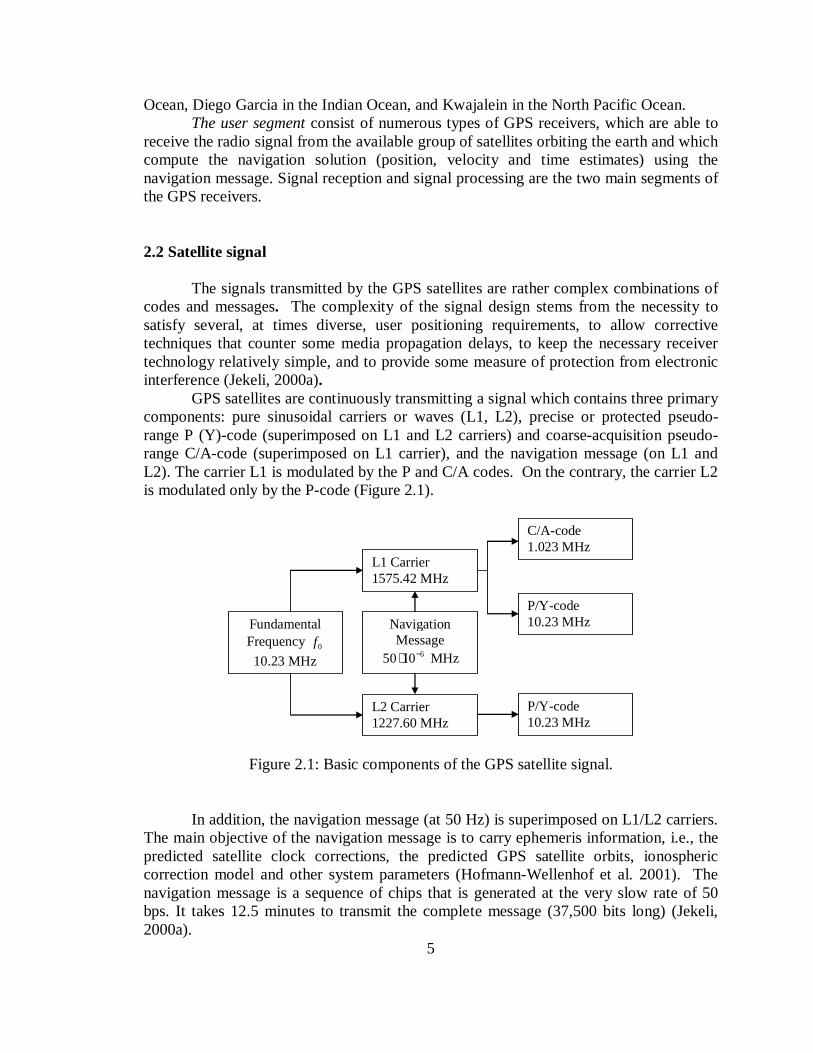
GPS satellites are continuously transmitting a signal which contains three primary components: pure sinusoidal carriers or waves (L1, L2), precise or protected pseudo-range P (Y)-code (superimposed on L1 and L2 carriers) and coarse-acquisition pseudo-range C/A-code (superimposed on L1 carrier), and the navigation message (on L1 and L2). The carrier L1 is modulated by the P and C/A codes. On the contrary, the carrier L2 is modulated only by the P-code (Figure 2.1).

Fundamental Frequency 0f

10.23 MHz

L1 Carrier 1575.42 MHz

C/A-code 1.023 MHz

P/Y-code 10.23 MHz

L2 Carrier 1227.60 MHz

P/Y-code 10.23 MHz

Navigation Message

650 10−⋅ MHz

Figure 2.1: Basic components of the GPS satellite signal.

In addition, the navigation message (at 50 Hz) is superimposed on L1/L2 carriers. The main objective of the navigation message is to carry ephemeris information, i.e., the predicted satellite clock corrections, the predicted GPS satellite orbits, ionospheric correction model and other system parameters (Hofmann-Wellenhof et al. 2001). The navigation message is a sequence of chips that is generated at the very slow rate of 50 bps. It takes 12.5 minutes to transmit the complete message (37,500 bits long) (Jekeli, 2000a).

6

Thus the total signal transmitted by the satellite is given by the sum of the three sinusoids, two for the two codes (C/A and P) superimposed on L1 carrier and one for the P-code superimposed on L2 carrier. Each satellite transmits a unique C/A-code and a unique one-week long segment of P-code, reinitialized weekly at Saturday/Sunday midnight. The P-code is currently not available to the civilian users, due to the implementation of the Anti-Spoofing (AS), where the W-code is used to encrypt the P-code into the Y-code.

In order to recover the carrier L2 when the Anti-Spoofing (AS) is present, several methods have been proposed (Hofmann-Wellenhof et al. 2001; Brzezinska, 2001):

Codeless squaring technique is based on auto-correlating the incoming L2 signal, which results in an un-modulated carrier with twice the carrier frequency. The PRN modulation and the navigation message are lost, since the signal is multiplied by itself. In other words, the squaring technique is independent of PRN codes. Here, the signal-to-noise ratio (SNR) is substantially reduced in comparison with the code correlation technique.

Cross-correlation technique is based on the fact that the unknown Y-code is identical on both carriers (L1 and L2), which permits obtaining a difference (cross-correlation) between them. Here, the Y-code on L2 is slightly slower than the Y-code on L1 (due to the frequency propagation of the electronic wave through the ionosphere). In comparison with the code correlation technique an SNR degradation of 27 dB (decibel) occurs.

Code correlation with squaring allows the correlation between the Y-code and the carrier L2 with the generated replica of the P-code, followed by low-pass filtering and squaring to remove the code modulation. This technique is possible because the Y-code originates from a module two sum of the P-code and the encrypting W-code. In comparison with the code correlation technique an SNR degradation of 17 dB (decibel) occurs.

Z-tracking technique consists of the separate correlation between the Y-code on the carriers L1/L2 and the locally generated replica of the P-code. Due to the fact that both frequencies contain the encrypted code, the signal integration allows for the estimation of the encrypted signal bit for each of them, which is subsequently fed to the other frequency. In comparison with the squaring technique the SNR is improved by 3 dB. However, in comparison with the code correlation technique an SNR degradation of 14 dB (decibel) occurs.

According to the manufacturers, the GPS receivers analyzed in this report use different techniques under AS; for some of the receivers this information is not available to the author (e.g. Trimble 4000 SSE and SSI, Topcon/JPS Legacy and Trimble 4700), while, based on manufacturers specifications, it can be stated that Leica 9500 uses narrow correlation technique and Ashtech Z-S uses Z-tracking technique. The Z-tracking technique (theoretically) offers the best performance of the receiver under the AS presence and less degradation on the SNR (Hofmann-Wellenhof et al. 2001) in comparison with the other techniques. Moreover, in all of codeless (semi-codeless) techniques of L2 signal recovery (except for squaring), some interaction between tracking loops on L1 and L2 is introduced, which indicates that some correlation may result.

7

It is still expected by civilian users the called L5 (transmitted on 1176.45 MHz), which will be a "safety-of-life" signal. It will be similar in structure to the current military code and will be approximately four times stronger than the L1 signal. The L5 signal will be implemented on the modified Block IIF satellites. For the military, there will be a new M-code line, with increased power and the ability to jam enemy use (http://nationaldefense.ndia.org/). 2.3 GPS observables

The three fundamental GPS observables are the pseudo-range, carrier phase and Doppler measurement, and they are briefly explained in the following sections. 2.3.1 The pseudo-range observable

The pseudo-range observable is the geometric range between the transmitter (GPS satellite) and the receiver (GPS receiver) based on time measurement scaled by the speed of light, and disturbed by the lack of synchronization between the satellite and receiver clocks, and the propagation media (Hofmann-Wellenhof et al. 2001). It is known that:

k ki it t t∆ = − (2.1)

where kit∆ is the difference (in time) between the emitted signal by a satellite and the

received one by the receiver, it is the reading of the receiver clock at signal reception

time, kt is the reading of the satellite clock at signal emission time (transmitted via PRN code), i and k refer to receiver and satellite, respectively.

However, some delays (with respect to the GPS system time) of the clocks for the satellite ( kδ ) and for the receiver (iδ ) must be considered. Then (2.1) can be

transformed in: [ ( ) ] [ ( ) ]k k k

i i it t GPS t GPSδ δ∆ = − − − (2.2)

It is important to point out that the satellite clock information (known) is transmitted via navigation message in the form of three polynomial coefficients ( 0 1 2, ,a a a ) with a reference time ct . Due to this fact, the satellite clock bias (at epoch t)

can be computed by (Hofmann-Wellenhof et al. 2001). 2

0 1 2( ) ( ) ( )kc ct a a t t a t tδ = + − + − (2.3)

Using (2.1) and simplifying (2.2) results in: ( )k k k

i i it t GPS δ∆ = ∆ + ∆ (2.4)

where k ki iδ δ δ∆ = − (the term k

iδ∆ is equal to the receiver clock delay (iδ ) when the kδ

correction is applied). Multiplying the speed of light by the time interval kit∆ and using (2.4) the general

equation of a pseudo-range can be given by (Hofmann-Wellenhof et al. 2001):

8

( )k k k k k ki i i i i iR c t c t GPS c cδ ρ δ= ∆ = ∆ + ∆ = + ∆ (2.5)

where kiR is the pseudo-range corrected for satellite clock bias, c is the speed of light,

kiρ is the geometric distance between satellite (k) and receiver (i), calculated from the

true signal travel time 2.3.2 The carrier phase observable

The carrier phase observable is the difference between the phases of a carrier signal received from the satellite and a reference signal generated by the receiver’s internal oscillator (replica). The basic equation of the carrier phase measurement can be obtained as follows (Hofmann-Wellenhof et al. 2001).

It is well known that the circular frequency (f ) results from differentiating the phase (ϕ ) with respect to time (t):

dt

df

ϕ= (2.6)

Consequently, the phase (ϕ ) results by integrating the circular frequency (f )

between the epochs 0t and 1t . 1

0

t

t

fdtϕ = ∫ (2.7)

The phase equation (2.8) for electromagnetic waves (as observed at the receiving site) it can be obtained by using (2.6) and taking into account the following assumptions (Hofmann-Wellenhof et al. 2001):

−=−=c

tfttfρϕ ρ )( (2.8)

1. Constant frequency is assumed, and initial phase 0)( 0 =tϕ is considered.

2. The time span ρt , which the signal needs to propagate through the distance ρ

from the satellite to the receiver, is also considered. Then, according to (2.8) the following phase equations are:

0( )k

k k k kit f t fc

ρϕ ϕ= − − and 0( )i i it f tϕ ϕ= − (2.9)

where ( )k tϕ is the phase of the received and reconstructed carrier with frequency kf ,

( )i tϕ is the phase of a reference carrier generated in the receiver (i) with frequencyif , t is

an epoch in the GPS time (computed from the initial epoch 00 =t ).

Therefore, the initial phases 0kϕ and 0iϕ (caused by clock errors) are equal to:

0k k kfϕ δ= and 0i i ifϕ δ= (2.10)

Subsequently, using (2.9) the beat phase ( )ki tϕ is given by:

( ) ( ) ( )k ki it t tϕ ϕ ϕ= − (2.11)

9

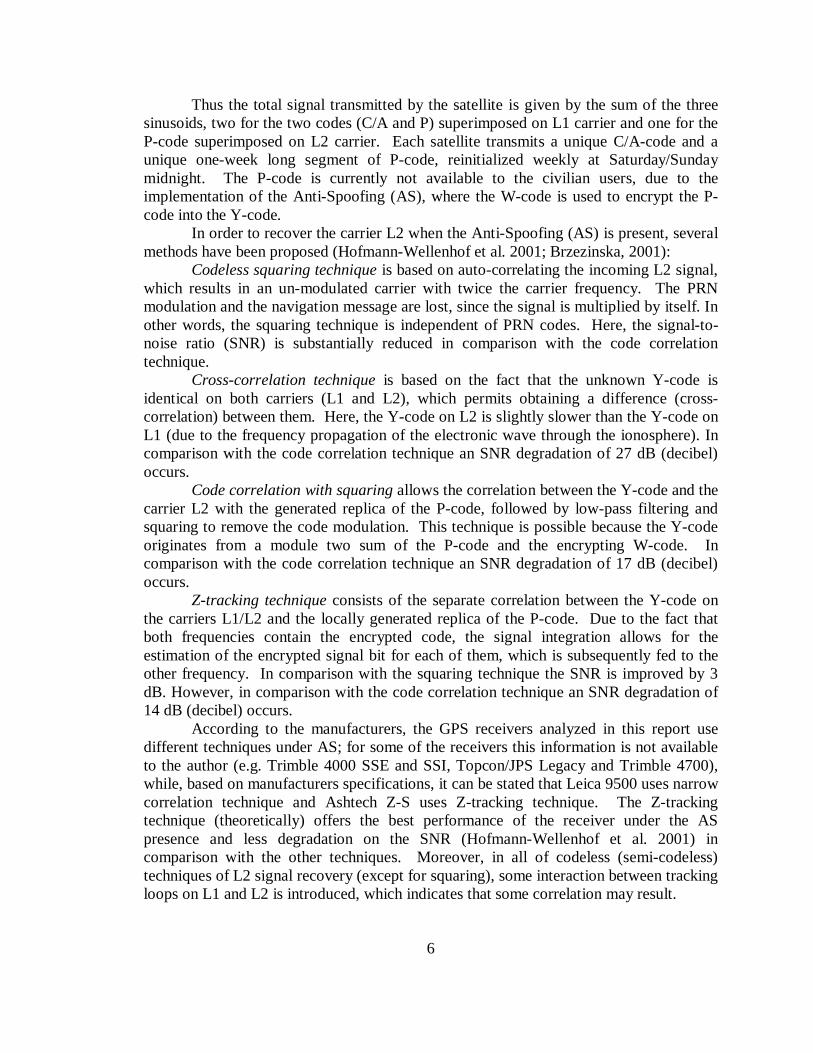
Substituting (2.9) and (2.10) into (2.11), and simplifying results:

( ) ( )k

k k k k kii i i it f f f f f t

c

ρϕ δ δ= − − + + − (2.12)

Some terms in (2.12), such as the frequency error ( )kif f t− and the clock errors

ranges are normally neglected since their influence is not considered very significant; thus, (2.12) can be rewritten as:

( )k

k kii it f f

c

ρϕ δ= − − ∆ (2.13)

where: k ki iδ δ δ∆ = − (introduced before) (2.14)

Furthermore, (2.13) will be transformed into (2.15) when we switch on a receiver (at epoch 0t ); in other words, the instantaneous fractional beat is measured and the initial number of the full cycles, called ambiguity, N, is “unknown”.

0( )k k t k

i i t it Nϕ ϕ= ∆ + (2.15)

where kiϕ∆ - the measurable (fractional) phase at epoch t augmented by the number of

ambiguities N, (since the initial epoch ( 00 =t )).

Finally, substituting (2.15) into (2.13) and denoting the negative observation quantity by k k

i iϕΦ = −∆ , the basic equation of a carrier phase measurement between the satellite (k) and the receiver (i) is given by (Hofmann-Wellenhof et al. 2001):

1k k k k ki i i if Nρ δ

λΦ = + ∆ + (2.16)

where kiΦ is the carrier phase observation, k

iρ is the geometric distance between the

satellite (k) and the receiver (i), kiN is the carrier phase integer ambiguity, λ is the

carrier wavelength (f

c=λ ), f - nominal frequency ( kf f= ), c- the speed of light.

2.3.3 The Doppler observable

The Doppler measurement is a measure of the carrier phase rate. The general equation for the observed Doppler scaled to the range rate can be written according to (Hofmann-Wellenhof et al. 2001) as follows:

. . .k k k ki i i iD cλ ρ δ= Φ = + ∆ (2.17) kiD is the Doppler measurement, dot above the terms indicates derivatives with

respect to time, (. k

ic δ∆ ) is the time derivative of the combined clock bias, and the other terms are rates of the measurements explained earlier.

10

2.4 GPS errors and their effects on the GPS position

When we talk about GPS point positioning, it is important to keep it mind the presence of several errors associated with the GPS measurements. Some of them are said to be random and some are non-random in nature. A brief description of the errors is presented in the following sections. 2.4.1 Satellite and receiver clock bias

The satellite clock bias is a systematic error; it is modeled and transmitted in the navigation message. The receiver clock bias is the difference between the GPS time and the receiver clock time; it is unknown and it can be estimated together with the receiver’s position or velocity. However, using an appropriate linear combination of GPS observables (Differential GPS), both satellite and receiver clock biases can be eliminated. 2.4.2 Satellite orbital errors

It is well known that the broadcast orbital parameters are imperfect, and due to this fact they give an incorrect satellite location. According to Bowen, [1986] the expected contribution of the satellite orbital errors could reach about 2 m for 24 hours prediction. The forces, in order of their significance, that contribute to perturbations in the satellite orbit error are parameterized as: gravity, radiation pressure, atmosphere effects, geoid modeling, solid earth and ocean tides. For more information about satellite orbital errors, the reader is referred to the International GPS Service for Geodynamics (IGS) website: http://igscb.jpl.nasa.gov.

2.4.3 Multipath errors

Multipath is due to the fact that the signal from the satellite reaches the GPS antenna via multiple paths (direct and indirect paths). The primary causes of this error are the set of reflecting surfaces in the receiver’s neighborhood. Its magnitude tends to be random and unpredictable, and it can also reach 1-5 cm for phases and 10-20 m for code pseudo-ranges. Multipath can be largely reduced by careful antenna location (avoiding reflective objects) and proper antenna design (e.g., proper signal polarization, choke-ring or ground plane antennas) (Langley, 1997). A secondary method to mitigate multipath effects is the use of digital filtering (Bletzaker, 1985). 2.4.4 Antenna phase center offset

The physical (geometric) center of the antenna usually does not coincide with the phase center (electrical center) of the antenna. Moreover, the phase centers for L1 and

11

L2 usually do not coincide, and different types of GPS antennas also have different locations of their phase centers. The antenna phase center offset can be divided into two parts: (1) a constant offset that can easily be taken into account by performing laboratory test, and (2) the variation offset, however, that depends on the elevation, azimuth, intensity, and type of the GPS signal. It is important to mention here that the systematic variation of this offset is difficult to model since it differs from one antenna to another. Nevertheless, models for antenna offsets were proposed based on the azimuth and elevation of the satellite signal (Schupler et al. 1991). 2.4.5 Ionosphere errors

By definition, the ionosphere is the atmospheric layer extending for about 50-1000 km above the Earth’s surface. The ionospheric conditions can vary significantly during the course of the day; the effect of the ionosphere is less intense at night. Due to the presence of free-electrons in this layer, a delay in the GPS code pseudo-range and an advance in the carrier phase pseudo-range are observed. The Total Electron Content (TEC), along the GPS signal path, determines the effect of the ionosphere. The TEC depends on an 11-year sunspot cycle (the highest ionospheric activity for the current cycle was around Fall 2000), seasonal variations, elevation and azimuth of the satellite, and the location of the receiver. Very rapidly changing ionospheric conditions might cause GPS losses of lock, especially on the L2 frequency under Anti-Spoofing (AS). The estimated maximum rate-of-change of ionospheric delay, under conditions where tracking is still possible, is about 19 cm per second, which corresponds to about 1 cycle on L1 (Gourevitch, 1996).

Several methods are used to eliminate the ionosphere errors. The most common is to use a linear combination of both GPS frequencies (L1 and L2), for more details about the so-called ionosphere-free combination in the single or double-difference mode the reader is referred to Hofmann-Wellenhof et al. 2001. Another method used to reduce the ionosphere errors is based on the broadcast ionospheric parameters. These parameters model the effect of the ionosphere on the GPS signal, but can account only for ~50 % of the total effect. 2.4.6 Troposphere errors

The tropospheric layer extends up to 50 km above the earth surface. In contrast to the ionosphere, troposphere errors are frequency independent. For this reason, the elimination of the tropospheric effect by using dual frequency receivers is not possible. Similar to the ionosphere effect, the propagation delay of GPS signals depends on the atmospheric conditions and satellite elevation angle. Troposphere errors propagate into station coordinates estimates with the point positioning and also relative positioning. The tropospheric effects can be divided into dry and wet refractivity.

The dry component, which is proportional to the density of the gas molecules in the atmosphere and changes with their distribution, represents about 90% of the total

12

tropospheric refraction, and it can be accurately modeled to about 2-5% that corresponds to 4 cm in the zenith direction using surface measurements such as pressure and temperature (Leick, 1990). The wet refractivity is due to the polar nature of the water molecules and the electron cloud displacement. It is more difficult to model the wet atmosphere (even thought it accounts only for 10 % of the total effect) since variations of the water vapor in time and space are present. Nevertheless, proper modeling has been derived in order to estimate 90-95 % of this effect (e.g., Modified Hopfied Model by Goad and Goodman, 1974). It is important to mention that, the tropospheric refraction as a function of the satellite’s zenith distance is usually expressed as a product of a zenith delay and a mapping function. According to Brunner and Welsch, [1993], the lower the elevation angle of the incoming GPS signal, the more it is affected by the atmosphere. Therefore, GPS observations from satellites with elevation angles below 15 degrees are usually avoided. The troposphere effects ranges between 2 m delay in the zenith to about 25 m at 5 degrees elevation angle. Use of double differencing (DD) can eliminate the troposphere errors for short baselines. In contrast, for long baselines the DD tropospheric errors can be modeled as a part of the estimation process. 2.4.7 Relativistic errors

The relativistic effect in GPS is considered twofold. One is due to the fact that the satellite is moving and the gravitational field exerts a direct relativistic perturbation on the satellite orbit. Secondly, the gravity field directly affects the satellite clock’s frequency, at the order of 1010− . The geometry between the station, satellite and geocenter is a very important fact to consider for dynamics and propagation of relativistic errors. Circular orbits are the basis for computing the prevailing portion of the relativistic errors. It is known that, for single-phase measurements the maximum effect in the range is about 19 mm, and it can be significantly reduced to the order of 0.001 ppm for relative positioning when DGPS is available, Ashby (1987). Table 2.1 shows a summary of the one-sigma magnitudes of the different errors that affect GPS observations under the assumption that SA is not operating (Parkinson et al. 1996).

Table 2.1: Summary of GPS errors sources with no SA present.

One-sigma error (m)

Error source Bias Random Total Ephemeris data 2.1 0.0 2.1 Satellite clock 2.0 0.7 2.1 Ionosphere 4.0 0.5 4.0 Troposphere 0.5 0.5 0.7 Multipath 1.0 1.0 1.4 Receiver measurement 0.5 0.2 0.5 User equivalent range error (UERE), rms 5.1 1.4 5.3 Filtered UERE, rms 5.1 0.4 5.1 VERTICAL ONE-SIGMA ERRORS-VDOP = 2.5 12.8 HORIZONTAL ONE-SIGMA ERRORS- HDOP = 2.0 10.2

13

As can be seen in Table 2.1, the dominant error is usually the ionosphere. The termrms is the statistical ranging error (one-sigma) that represents the total of all contributing sources.

If we consider the presence of some of the errors explained above, the pseudo-range equation (2.5) can be rewritten more generally as (Hofmann-Wellenhof et al. 2001):

( ) ( ) ( )( ) ( ) ( )k k k k k k ki i i ion i trop i mult i iR t t d d d c tρ δ ε= + + + + ∆ + (2.18)

where kiR is the pseudo-range corrected for satellite clock bias, k

iρ is the geometric

distance between the satellite and the receiver, ( )ki iond and ( )

ki tropd are delays imparted by

the ionosphere and troposphere respectively, ( )ki multd is the pseudo-range multipath error,

c is the speed of light, kiδ∆ is the receiver’s clock bias, kiε is the random noise.

Similarly for the carrier phase, Equation (2.16) can be rewritten more generally as (Hofmann-Wellenhof et al. 2001):

( ) ( ) ( )

1( ) ( ) ( )k k k k k k k k k

i i i i ion i trop i mult i it t N d d d f tρ δ ελ

Φ = + − + + + ∆ + (2.19)

where kiΦ is the carrier phase observation (in cycles), λ is the carrier wavelength, kiN is

the carrier phase ambiguity 2.5 GPS coordinate systems

Basic definitions about coordinate systems are needed to explain the positioning principles of the GPS system. Since in space geodesy, the objects are moving with respect to the reference frames, and considering the fact that frames are also moving in space, the time information related to the epoch of observation and the reference time at which the frame is defined, must be specified. For this reason, it is important to understand the difference between a reference system and a reference frame, since these concepts apply throughout the discussion of coordinate systems. According to the International Earth Rotation Service (IERS), a “Reference System is defined as the set of prescriptions and conventions together with the modeling required to define at any time a triad of coordinate axes”, and a “Reference Frame realizes the system by means of coordinates of definite points that are accessible directly by occupation or by observation”. For more information the reader is referred to “Earth Rotation: Theory and Observation”, by Moritz and Mueller (1987). Two different types of coordinate systems are outlined here: Celestial and Terrestrial. The Celestial (space fixed, or inertial) is needed to describe the satellite motion in space. The Terrestrial (earth fixed) is used to obtain position coordinates on the ground. GPS uses an Earth-Fixed global reference frame called World Geodetic System (WGS-84) as reference. The WGS84 coordinate system (geocentric) is a conventional terrestrial reference system (CTRS), which coincides with the center of mass being defined for the whole earth including oceans and atmosphere. The WGS-84 is now equivalent to the ITRF00, after 1994, 1997 and 2000 refinements of the WGS-84 (adjustment of the best fitting 7-parameter transformation). The geodetic coordinates can be transformed to Earth

14

Centered Earth Fixed (ECEF) Cartesian coordinate system by the well-known formula:

( )2

( ) cos cos

( )cos sin

1 sinECEF

x N h

y N h

z N e h

ϕ λϕ λ

ϕ

+ = + − +

(2.20)

where ϕ is the geodetic latitude, λ is the geodetic longitude, h is the ellipsoidal height, N is the radius of curvature of the prime vertical, e is the ellipsoidal eccentricity. 2.6 Differential GPS (DGPS)

DGPS is a real-time or post-processing positioning technique where a stationary GPS receiver (base) is placed at a well-known location and the relative position of the rover (or other stationary receiver) with respect to the base is determined (Hofmann-Wellenhof et al. 2001). DGPS is applied in geodesy and surveying, and it usually involves at least one or more GPS base stations. A common approach used to eliminate or reduce common errors is the formation of linear combinations of GPS measurements (e.g., single and double differences). This can be achieved by combining data from two receivers observing the same satellite a second satellite simultaneously.

2.6.1 Single-difference observations

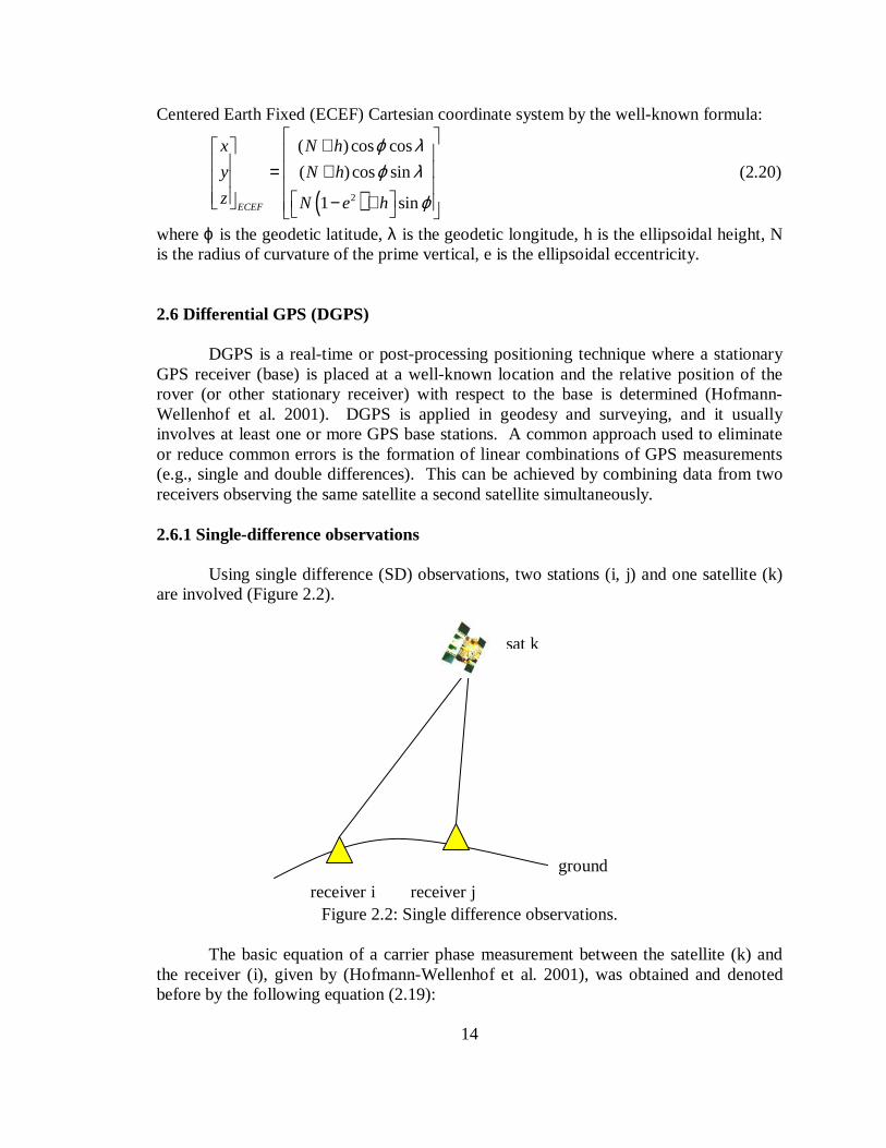
Using single difference (SD) observations, two stations (i, j) and one satellite (k) are involved (Figure 2.2).

Figure 2.2: Single difference observations. The basic equation of a carrier phase measurement between the satellite (k) and

the receiver (i), given by (Hofmann-Wellenhof et al. 2001), was obtained and denoted before by the following equation (2.19):

sat k

receiver i receiver j

ground

15

( ) ( ) ( )

1( ) ( ) ( )k k k k k k k k k

i i i i ion i trop i mult i it t N d d d f tρ δ ελ

Φ = + − + + + ∆ +

If we substitute (2.14) into the previous equation (2.19) and shifting the satellite clock bias (given by 2.3) to the left side of the equations yields:

( ) ( ) ( )

1( ) ( ) ( ) ( )k k k k k k k k k k

i i i i ion i trop i mult i it f t t N d d d f tδ ρ δ ελ

Φ + = + − + + + +

or (2.21)

( ) ( ) ( )

1( ) ( ) ( ) ( )k k k k k k k k k k

j j j j ion j trop j mult j jt f t t N d d d f tδ ρ δ ελ

Φ + = + − + + + +

Two-phase equations for two points (i, j), are given in (2.21). Differencing these two equations results in a single-difference equation of the form:

, , , , ( ) , ( ) , ( ) , ,

1( ) ( ) ( )k k k k k k k k

i j i j i j i j ion i j trop i j mult i j i jt t N d d d f tρ δ ελ

Φ = + − + + + + (2.22)

with

,k k ki j j iN N N= −

, ( ) ( ) ( )i j j it t tδ δ δ= −

, ( ) ( ) ( )k k ki j j it t tΦ = Φ − Φ

, ( ) ( ) ( )k k ki j j it t tρ ρ ρ= −

The Equation (2.22) represents the final form of the single-difference equation (Hofmann-Wellenhof et al. 2001). Here, the satellite clock bias ( ( )k tδ ) has canceled compared to the phase equation (2.21). 2.6.2 Double-difference observations

Using double-difference (DD) observations, two stations (i, j) and two satellites (k, l) are involved (see Figure 2.3).

Figure 2.3: Double difference observations.

sat k sat l

receiver i receiver j

ground

16

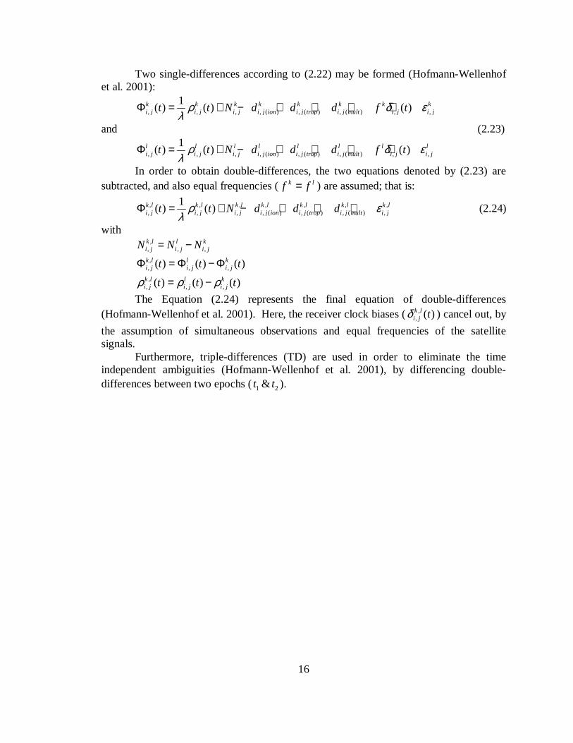
Two single-differences according to (2.22) may be formed (Hofmann-Wellenhof et al. 2001):

, , , , ( ) , ( ) , ( ) , ,

1( ) ( ) ( )k k k k k k k k

i j i j i j i j ion i j trop i j mult i j i jt t N d d d f tρ δ ελ

Φ = + − + + + +

and (2.23)

, , , , ( ) , ( ) , ( ) , ,

1( ) ( ) ( )l l l l l l l l

i j i j i j i j ion i j trop i j mult i j i jt t N d d d f tρ δ ελ

Φ = + − + + + +

In order to obtain double-differences, the two equations denoted by (2.23) are subtracted, and also equal frequencies (k lf f= ) are assumed; that is:

, , , , , , ,, , , , ( ) , ( ) , ( ) ,

1( ) ( )k l k l k l k l k l k l k l

i j i j i j i j ion i j trop i j mult i jt t N d d dρ ελ

Φ = + − + + + (2.24)

with ,

, , ,k l l ki j i j i jN N N= −

,, , ,( ) ( ) ( )k l l k

i j i j i jt t tΦ = Φ − Φ ,

, , ,( ) ( ) ( )k l l ki j i j i jt t tρ ρ ρ= −

The Equation (2.24) represents the final equation of double-differences (Hofmann-Wellenhof et al. 2001). Here, the receiver clock biases ( ,

, ( )k li j tδ ) cancel out, by

the assumption of simultaneous observations and equal frequencies of the satellite signals.

Furthermore, triple-differences (TD) are used in order to eliminate the time independent ambiguities (Hofmann-Wellenhof et al. 2001), by differencing double-differences between two epochs (1 2&t t ).

17

CHAPTER 3

THE GPS RECEIVER AND RANDOM PROCESS

In this Chapter, we provide the background information about the GPS receivers, since our stochastic analysis is focused on the performance of six GPS receivers of different types and makes. An overview of random processes is also outlined, where a description of the stochastic aspects (basis of the stochastic analysis) is provided. 3.1 GPS receiver overview

For the last twenty years GPS instrumentation (for military and civilians) has evolved through several stages of design and implementation. A very considerable improvement in the accuracy and reliability of position and time determination has been achieved, including a modularization and miniaturization of the GPS receivers. By far, the majority of the GPS receivers manufactured today are of the C/A-code, single frequency type. However, when high precision is required (e.g. geodetic applications), dual frequency phase observations are standard features. In addition, GPS World (January 2001, Vol.12 No.1 pp.32-47) lists 518 different types of GPS receivers from 67 manufacturers. 3.2 GPS receiver performance

In general, the performance of a GPS receiver depends on several factors such as, the number of satellites visible, observation conditions, occupation time, possible obstructions, baseline length and the atmospheric conditions (Brzezinska, 2001). Thus, if we want to achieve good results from GPS measurements, it is important to understand what we can expect under those conditions. 3.2.1 GPS receiver noise

As mentioned before, the primary consideration behind the study presented in this thesis is related to the estimation and interpretation of the level of measurement noise (based on SD-residuals) for six different types of GPS receivers. For this reason, GPS receiver noise characteristics must be taken into account. It is well known that, due to the fact that GPS receivers are measuring instruments, some level of noise is always associated with them. The most basic kind of noise affecting the GPS receivers is the thermal noise, which is an electrical current generated by the electron’s random motion. A concise overview of the causes and sources of this noise (thermal) contaminating GPS observable is given by (Langley, 1997). The commonly used measure of the received

18

signal strength is called signal-to-noise-ratio1 (SNR). In case of the radio frequency (RF) and intermediate frequency (IF), the traditionally used measure of the signal’s strength is the carrier-to-noise-power density ratio2 ( 0/C N ). The term ( 0/C N ) is considered a

primary parameter describing the GPS receiver performance, and its values determine the precision of the pseudo-range and carrier phase measurements (Brzezinska, 2001). 3.3 Main components of a GPS receiver

As mentioned before, the number of types of GPS receivers is very large, but one might still pose a question: Are all the GPS receivers essentially the same, apart from functionality and user software? The general answer is yes; all GPS receivers consist of essentially the same functional blocks, even though their implementations may differ (Brzezinska, 2001).

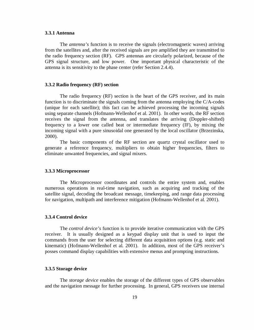
According to Hofmann-Wellenhof et al. 2001, the primary components of a generic GPS receiver (Figure 3.1) are: antenna, radio frequency (RF) section, microprocessor, control/storage device, and power supply.

Figure 3.1: Basic conceptual architecture of a GPS receiver. 1 It is defined as a ratio of the received signal’s power, S, and the noise power, n, measured at the same time and place in a circuit, made on signal at band occupied by the signal after demodulation. 2 It is the ratio of the power level of the signal carrier to the noise power in a 1 Hz bandwidth

RF Section

Micro-Processor

Storage Device

Power Supply

Antenna

Control Device

19

3.3.1 Antenna

The antenna’s function is to receive the signals (electromagnetic waves) arriving from the satellites and, after the received signals are pre amplified they are transmitted to the radio frequency section (RF). GPS antennas are circularly polarized, because of the GPS signal structure, and low power. One important physical characteristic of the antenna is its sensitivity to the phase center (refer Section 2.4.4). 3.3.2 Radio frequency (RF) section

The radio frequency (RF) section is the heart of the GPS receiver, and its main function is to discriminate the signals coming from the antenna employing the C/A-codes (unique for each satellite); this fact can be achieved processing the incoming signals using separate channels (Hofmann-Wellenhof et al. 2001). In other words, the RF section receives the signal from the antenna, and translates the arriving (Doppler-shifted) frequency to a lower one called beat or intermediate frequency (IF), by mixing the incoming signal with a pure sinusoidal one generated by the local oscillator (Brzezinska, 2000).

The basic components of the RF section are quartz crystal oscillator used to generate a reference frequency, multipliers to obtain higher frequencies, filters to eliminate unwanted frequencies, and signal mixers. 3.3.3 Microprocessor

The Microprocessor coordinates and controls the entire system and, enables numerous operations in real-time navigation, such as acquiring and tracking of the satellite signal, decoding the broadcast message, timekeeping, and range data processing for navigation, multipath and interference mitigation (Hofmann-Wellenhof et al. 2001).

3.3.4 Control device The control device’s function is to provide iterative communication with the GPS

receiver. It is usually designed as a keypad display unit that is used to input the commands from the user for selecting different data acquisition options (e.g. static and kinematic) (Hofmann-Wellenhof et al. 2001). In addition, most of the GPS receiver’s posses command display capabilities with extensive menus and prompting instructions. 3.3.5 Storage device

The storage device enables the storage of the different types of GPS observables and the navigation message for further processing. In general, GPS receivers use internal

20

microchips, removable memory cards, cassette drives, etc. (Hofmann-Wellenhof et al. 2001). The storage capacity will depend on several aspects, such as the user needs, length of the data acquisition session, type of observable to be recorded, number of channels, etc. 3.3.6 Power supply

The power supply basically consists of AC or DC (internal rechargeable NiCd batteries, or external batteries such as, Lithium or Sealed Lead Acid batteries). The lower the power assumption of the receiver, the more survey time can be achieved from a single battery, and the less heavy load on the user going to the field. Moreover, lower power consumption also increases the life span of the electronics (Brzezinska, 2001). 3.4 GPS receiver classification

GPS receivers can be classified in several groups depending on several criteria (Seeber, 1993; Hofmann-Wellenhof et al. 2001). An early classification was into code correlation receiver technology and signal squaring receiver technology. This classification separates code-dependent receivers and code- free receivers. However, a better classification criteria takes into account data-types provided by receivers; namely C/A-code, C/A-code + L1 carrier phase, C/A-code + L1 carrier phase + L2 carrier phase, C/A-code + P-code + L1, L2 carrier phase, L1 carrier phase (not often used), and L1, L2 carrier phase (not often used). Furthermore, an important classification is related to the technical realization of the channels: multi-channel receiver, sequential receiver or multiplexing receiver. Last but not least, a classification with respect to the user community: military receiver, civilian receiver, navigation receiver, timing receiver and geodetic receiver, is also quite common. 3.5 Hardware tested

A brief background information (provided by the manufacturer) about the GPS receivers used for the GPS surveys (short/zero baseline) is outlined next: 3.5.1 Trimble 4000SSE GPS receiver

Trimble 4000SSE is a dual frequency geodetic grade GPS receiver. According to

the manufacturer, its performance criteria will depend on aspects, such as the number of satellites visible, occupation time, observation conditions, obstructions, baseline length and environmental effects (atmospheric conditions). It assumes five satellites (minimum) are tracked continuously with the recommended static surveying procedures using L1 and L2 signals at all sites. This GPS receiver is suitable for survey and mapping applications.

Some of the principal specifications (provided by the manufacturer) for Trimble

21

4000SSE are: size-24.8 × 28 × 10.2 cm, weight-3.1 kg, real-time differential GPS accuracy of 0.2 m + 1 ppm RMS, L1 C/A code, L1/L2 full-cycle carrier and fully operational during the AS presence. A view of Trimble 4000SSE is given in Figure 3.2, courtesy of Angel-GFZ Airborne Navigation and Gravity Ensemble & Laboratory.

Figure 3.2: Trimble 4000SSE front and rear view. 3.5.2 Trimble 4000SSI GPS receiver

Trimble 4000SSI is a 9-channel dual frequency geodetic grade GPS receiver.

According to the manufacturer, Trimble 4000SSI acquires low power satellite signals better, maintains a firm lock on signals once acquired, and provides superior tracking under conditions of radio interference, assuming at least 5 satellites are visible and PDOP < 4. This GPS receiver is normally used for post-processing of land surveys and mapping applications.

Some of the main specifications (provided by the manufacturer) for Trimble 4000SSI are: size-24.8 × 28 × 10.2 cm, weight-3.1 kg, real-time differential GPS accuracy ≤ 1m RMS, full cycle L1/L2 carrier phase, L1/L2 P-code and L1 C/A code during AS. Trimble 4000SSI is shown in Figure 3.3 below, courtesy of Trimble Surveying and Mapping Products (http://www.trimble.com).

Figure 3.3: Trimble 4000SSI.

22

3.5.3 Leica SR9500 GPS receiver

This is a 12-channel dual frequency geodetic grade GPS receiver. According to the manufacturer, Leica SR9500 can be used either as a reference station or as part of a roving unit for detailed surveying or stakeout. Up to 12 satellites can be tracked at any time, and the patented P-code-aided tracking provides the strongest signal for reliable tracking of satellites even under poor environmental conditions. It is an ideal receiver for geodetic and mapping applications (http://leica-geosystems.com).

The main tracking specifications (provided by the manufacturer) for Leica SR9500 are: full L1 carrier phase, P1 code or P-code aided under AS, full L2 carrier phase, P2 code, or P-code aided under AS, C/A code narrow correlation technique, fully independent L1 and L2 carrier-phase measurements, and fully independent, L1 and L2 pseudo-range for sub-metre differential positions. A view of this GPS receiver is shown in Figure 3.4, courtesy of Leica Geosystems.

Figure 3.4: Leica SR9500.

3.5.4 Topcon/JPS Legacy GPS receiver

Legacy is a dual-frequency, integrated geodetic grade GPS receiver. According to the manufacturer, its performance basically depends on its tracking abilities: it provides 40 L1 channels, 20 L1 + L2 channels, and it tracks L1/L2, C/A and P code and carrier signals. It is also capable of tracking both GPS and GLONASS (Russia’s Global Navigation Satellite System) constellations and maintains tracking abilities under harsh field environmental conditions. Legacy is suitable for geodetic and mapping applications (http://topconps.com).

Some of the principal specifications (provided by the manufacturer) for Legacy are: size-22.5 × 20.5 × 3.5 cm, weight-0.7 kg, real-time differential GPS accuracy of 2 ppm RMS, fully operational L1/L2 carrier phase, P1/P2 code under AS. An example of how this GPS receiver looks is presented in Figure 3.5, courtesy of Javad Positioning Systems.

23

Figure 3.5: Topcon/JPS Legacy.

3.5.5 Ashtech Z-Surveyor GPS receiver

The Ashtech Z-Surveyor is 12-channel dual-frequency geodetic grade GPS receiver. According to the manufacturer, accuracy for this GPS receiver assumes five visible satellites (at minimum). High-multipath areas, high PDOP values, and high atmospheric effects could affect its performance. It can be configured for a variety of survey applications including topographic mapping, geodetic control, stakeout or photogrammetry (http://www.ashtech.com).

Some of the main specifications (provided by the manufacturer) for Ashtech Z-surveyor are: size-7.5 × 18.2 × 20.6 cm, weight-1.6 kg, real-time differential GPS accuracy of <1 m (2 drms), full-wavelength carrier phase L1 and L2, uses z-tracking technique under AS. Ashtech Z-surveyor is illustrated in Figure 3.6, courtesy of Magellan Corporation/Ashtech Precision Products.

Figure 3.6: Ashtech Z-Surveyor. 3.5.6 Trimble 4700 GPS receiver

Trimble 4700 is a 9-channel, dual-frequency, geodetic grade GPS receiver. According to the manufacturer, the performance criteria for Trimble 4700 depend on the number of satellites visible, occupation time, observation conditions, obstructions, baseline length and environmental effects, and are based on favorable atmospheric

24

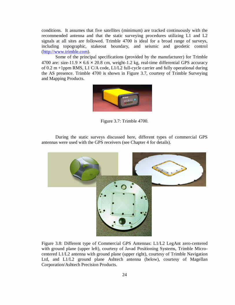
conditions. It assumes that five satellites (minimum) are tracked continuously with the recommended antenna and that the static surveying procedures utilizing L1 and L2 signals at all sites are followed. Trimble 4700 is ideal for a broad range of surveys, including topographic, stakeout boundary, and seismic and geodetic control (http://www.trimble.com).

Some of the principal specifications (provided by the manufacturer) for Trimble 4700 are: size-11.9 × 6.6 × 20.8 cm, weight-1.2 kg, real-time differential GPS accuracy of 0.2 m +1ppm RMS, L1 C/A code, L1/L2 full-cycle carrier and fully operational during the AS presence. Trimble 4700 is shown in Figure 3.7, courtesy of Trimble Surveying and Mapping Products.

Figure 3.7: Trimble 4700.

During the static surveys discussed here, different types of commercial GPS antennas were used with the GPS receivers (see Chapter 4 for details). Figure 3.8: Different type of Commercial GPS Antennas: L1/L2 LegAnt zero-centered with ground plane (upper left), courtesy of Javad Positioning Systems, Trimble Micro-centered L1/L2 antenna with ground plane (upper right), courtesy of Trimble Navigation Ltd, and L1/L2 ground plane Ashtech antenna (below), courtesy of Magellan Corporation/Ashtech Precision Products.

25

3.6 Random process 3.6.1 Overview

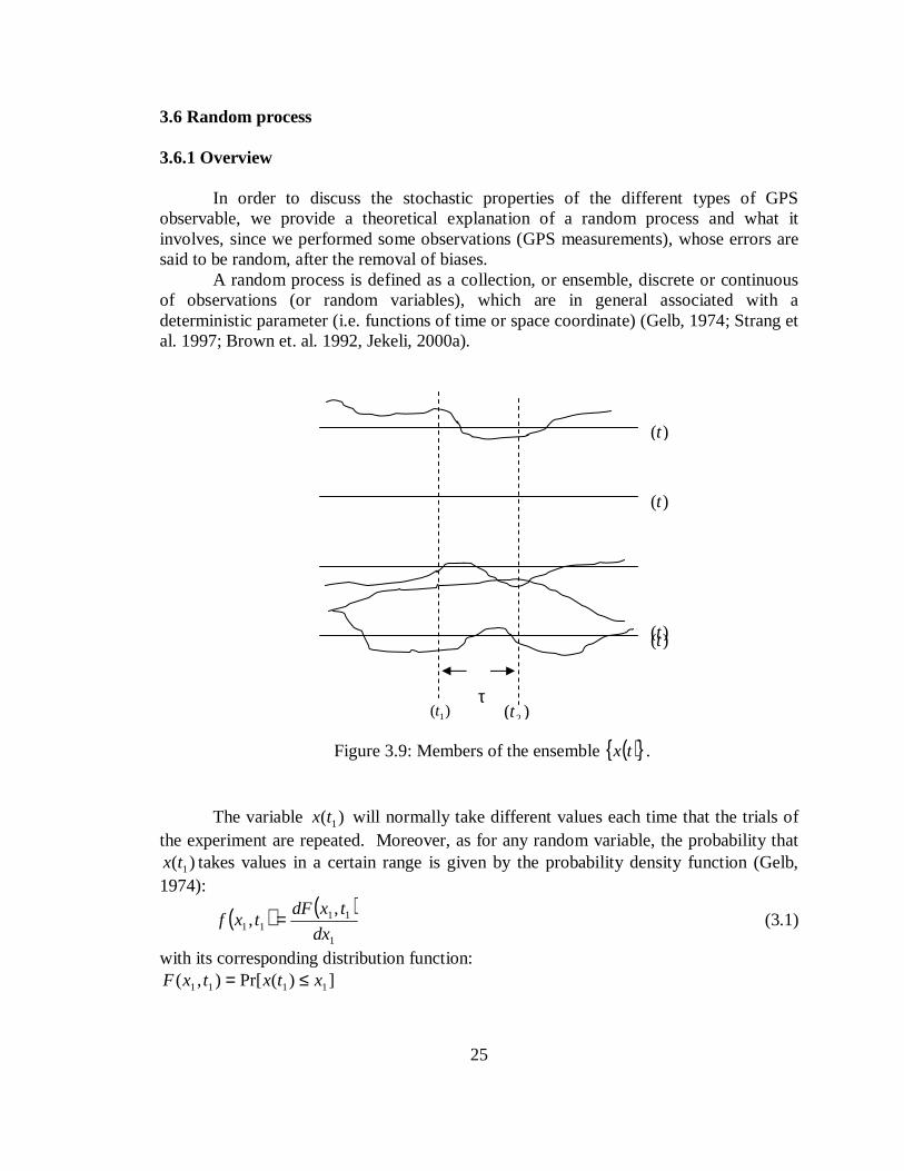
In order to discuss the stochastic properties of the different types of GPS observable, we provide a theoretical explanation of a random process and what it involves, since we performed some observations (GPS measurements), whose errors are said to be random, after the removal of biases.

A random process is defined as a collection, or ensemble, discrete or continuous of observations (or random variables), which are in general associated with a deterministic parameter (i.e. functions of time or space coordinate) (Gelb, 1974; Strang et al. 1997; Brown et. al. 1992, Jekeli, 2000a).

Figure 3.9: Members of the ensemble ( ){ }tx . The variable )( 1tx will normally take different values each time that the trials of

the experiment are repeated. Moreover, as for any random variable, the probability that )( 1tx takes values in a certain range is given by the probability density function (Gelb,

1974):

( ) ( )1

1111

,,

dx

txdFtxf = (3.1)

with its corresponding distribution function: ])(Pr[),( 1111 xtxtxF ≤=

)(t

)(t

)(t

)(t

)( 1t )( 2t τ

26

3.6.2 Gaussian random process

A Gaussian random process can be defined as one, where its joint probability distribution functions of all orders are multidimensional normal distributions. It is not sufficient that just the “amplitude” of the process be normally distributed; all high order density functions must also be normal (Strang et al., 1997 Gelb, 1974; Brown et. al., 1992). The probability density function of the normal distribution can be expressed as (Gelb, 1974):

( )2

2

1 1( ) exp

22p x x µ

σπσ = − −

(3.2)

where µ is the mean value, σ is the standard deviation (it measures the spread around the mean value).

Equation (3.2) is one-dimensional, the joint distribution of )( 1tx and 2( )x t is the bivariate normal distribution. On the other hand, higher-order joint distributions are given by the multivariate normal distribution.

Figure 3.10: Normal density( )p x (left) and its cumulative distribution ( )F x (right).

The normal density( )p x (bell-shaped) and its cumulative distribution ( )F x are shown in Figure 3.10 (Strang et al., 1997). It can also be seen from this figure that, the bell-shaped graph is symmetric around the middle point ( 0x µ= = ). The width of the bell-shaped graph is clearly governed by the second parameter σ , which stretches the x -axis and shrinks the y-axis (leaving the total area equal to 1). On the other hand, the other graph (right) shows the integral of the bell-shaped normal density. Here, the middle point x µ= has 0.50F = , which means that by symmetry, there is a 50-50 chance of an outcome below or above the mean. The interval denoted by the area between 1.96µ σ− and 1.96µ σ+ is considered as a 95% probability (x is less than two deviations from the mean). 3.6.3 Correlation functions

In the stochastic analysis based on static GPS measurements (zero baseline), we use the SD-residuals that represent random variables of a random process. In order

27

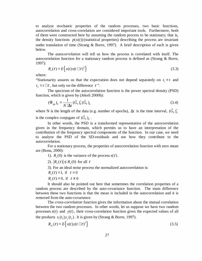
to analyze stochastic properties of the random processes, two basic functions, autocorrelation and cross-correlation are considered important tools. Furthermore, both of them were constructed here by assuming the random process to be stationary; that is, the density functions ( ( ))p x t (statistical properties) describing the process are invariant under translation of time (Strang & Borre, 1997). A brief description of each is given below.

The autocorrelation will tell us how the process is correlated with itself. The autocorrelation function for a stationary random process is defined as (Strang & Borre, 1997):

{ }( ) ( ) ( )TxR E x t x tτ τ= + (3.3)

where: “Stationarity assures us that the expectation does not depend separately on 1t t= and

2t t τ= + , but only on the difference τ ”. The spectrum of the autocorrelation function is the power spectral density (PSD)

function, which is given by (Jekeli 2000b): *1

( ) ( ) ( )gg k T k T kG GN t

Φ =⋅ ∆

⌢ɶ ɶ (3.4)

where N is the length of the data (e.g. number of epochs), t∆ is the time interval, *( )T kGɶ

is the complex conjugate of ( )T kGɶ . In other words, the PSD is a transformed representation of the autocorrelation

given in the frequency domain, which permits us to have an interpretation of the contribution of the frequency spectral components of the function. In our case, we need to analyze the PSD of the SD-residuals and see how they contribute to the autocorrelation.

For a stationary process, the properties of autocorrelation function with zero mean are (Bona, 2000):

1). (0)xR is the variance of the process( )x τ .

2). ( ) (0)x xR Rτ ≤ for all τ

3). For an ideal noise process the normalized autocorrelation is: ( ) 1,xR τ = if 0τ =

( ) 0,xR τ = if 0τ ≠

It should also be pointed out here that sometimes the correlation properties of a random process are described by the auto-covariance function. The main difference between these two functions is that the mean is included in the autocorrelation and it is removed from the auto-covariance.

The cross-correlation function gives the information about the mutual correlation between the two random processes. In other words, let us suppose we have two random processes )(tx and ( )y t , their cross-correlation function gives the expected values of all

the products 1 2( ) ( )i jx t y t . It is given by (Strang & Borre, 1997).

{ }( ) ( ) ( )TxyR E x t y tτ τ= + (3.5)

28

where 2 1t tτ = − . In addition, we point out three hypotheses concerning the positive correlation

between L1 and L2 carriers, while analyzing the stochastic properties of GPS observables (Bona et. al., 2000a):

1. The correlation can be due to the codeless or semi-codeless measurement technique used to circumvent the encryption of the P-code under the AS presence (refer to Section 2.1).

2. The correlation might result from a coupling of the L2 tracking loop with the L1 carrier phase.

3. The correlation may be caused by the internal data filtering (smoothing) that the receivers apply in order to reduce the measurement noise.

29

CHAPTER 4

ZERO BASELINE RESULTS

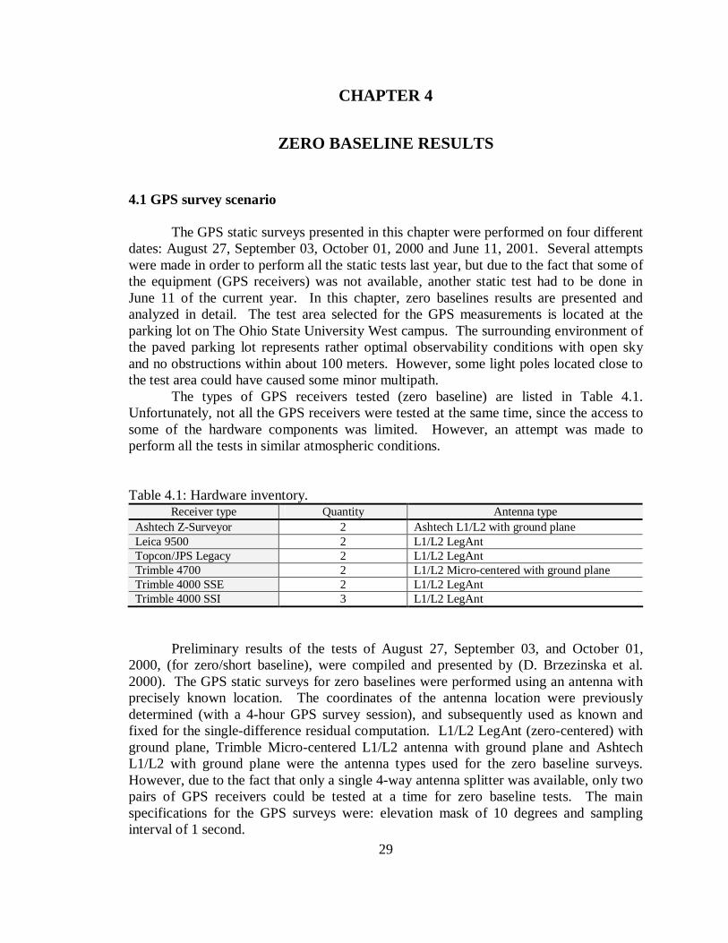
4.1 GPS survey scenario

The GPS static surveys presented in this chapter were performed on four different dates: August 27, September 03, October 01, 2000 and June 11, 2001. Several attempts were made in order to perform all the static tests last year, but due to the fact that some of the equipment (GPS receivers) was not available, another static test had to be done in June 11 of the current year. In this chapter, zero baselines results are presented and analyzed in detail. The test area selected for the GPS measurements is located at the parking lot on The Ohio State University West campus. The surrounding environment of the paved parking lot represents rather optimal observability conditions with open sky and no obstructions within about 100 meters. However, some light poles located close to the test area could have caused some minor multipath.

The types of GPS receivers tested (zero baseline) are listed in Table 4.1. Unfortunately, not all the GPS receivers were tested at the same time, since the access to some of the hardware components was limited. However, an attempt was made to perform all the tests in similar atmospheric conditions. Table 4.1: Hardware inventory.

Receiver type Quantity Antenna type Ashtech Z-Surveyor 2 Ashtech L1/L2 with ground plane Leica 9500 2 L1/L2 LegAnt Topcon/JPS Legacy 2 L1/L2 LegAnt Trimble 4700 2 L1/L2 Micro-centered with ground plane Trimble 4000 SSE 2 L1/L2 LegAnt Trimble 4000 SSI 3 L1/L2 LegAnt

Preliminary results of the tests of August 27, September 03, and October 01, 2000, (for zero/short baseline), were compiled and presented by (D. Brzezinska et al. 2000). The GPS static surveys for zero baselines were performed using an antenna with precisely known location. The coordinates of the antenna location were previously determined (with a 4-hour GPS survey session), and subsequently used as known and fixed for the single-difference residual computation. L1/L2 LegAnt (zero-centered) with ground plane, Trimble Micro-centered L1/L2 antenna with ground plane and Ashtech L1/L2 with ground plane were the antenna types used for the zero baseline surveys. However, due to the fact that only a single 4-way antenna splitter was available, only two pairs of GPS receivers could be tested at a time for zero baseline tests. The main specifications for the GPS surveys were: elevation mask of 10 degrees and sampling interval of 1 second.

30

4.2 GPS stochastic analysis and data processing technique

In this thesis, we will focus our attention on zero baseline test results, since the prime objective of this research is to perform an analysis of the stochastic properties of the different GPS observables based on their noise characteristics. The primary “observable” in our tests are SD-residuals on zero baseline, since all primary error source, like atmosphere, satellite clock, position errors and multipath are cancelled. Thus the receiver noise is the primary component of the measurement residuals and the receiver clock error can be estimated. Moreover, the statistics derived based on SD-residuals can be converted to statistics related to one-way (undifferenced) measurements, which will characterize a single receiver. It should be mentioned that performance analysis on zero baseline might be too optimistic, as opposed to the short baseline scenario, which provides a full valuation of the practical performance of the GPS receiver (Bona, 2000). However, only on zero baseline the noise of the observables can be assumed as coming from the receiver only. The stochastic analysis was based on single-difference residuals for high and low satellites, since the elevation angle is an important factor to consider with respect to the GPS measurements (Euler and Goad, 1991; Tiberius et al. 1999; Bona, 2000).

GPS measurements were collected for about 4-5 hours in order to determine the exact location of the antenna (zero baseline). Trimble Geomatics Office was used to process the data collected during the field measurements. Before the data processing all the data sets were converted to the RINEX format (Gurtner, 1994).

The receiver noise level is evaluated (quantified) by a statistical variance component estimation technique. Single difference residuals coming from the least squares adjustment are used, as explained below: It should be mentioned here that the receiver noise (i.e. observables noise) is measured by the square root of the autocorrelation at zero lag.

The linearized Gauss-Markov Model is given by y A eξ= + (4.1)

where y is the observation vector, A is the design matrix of the partial derivatives (“Jacobian Matrix”), ξ is the unknown vector, e is the error vector.

Under the assumption that SD-residuals on zero baseline do not contain satellite clock errors, atmospheric errors or multipath effects, the single-difference equation, previously denoted by (2.22), can be rewritten as:

, , , , ,

1( ) ( ) ( )k k k k k

i j i j i j i j i jt t f t Nρ δ ελ

Φ = + + + (4.2)

Analogous for pseudo-ranges:

, , ,( ) ( ) ( )k k ki j i j i jR t t f t eρ δ= + + (4.3)

Then, our system of equations according to our model (4.1), is set up using (4.2) and (4.3) as follows:

• For carrier phases:

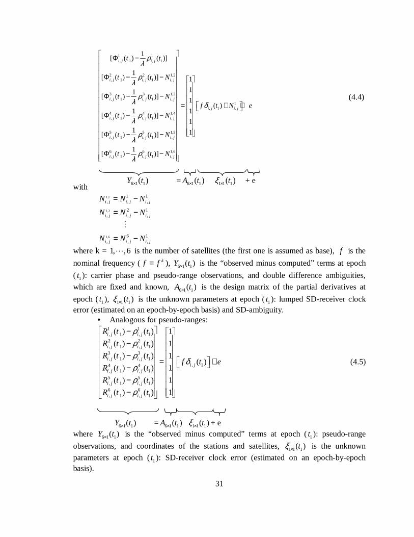
31

1 1, 1 , 1

2 2 1,2, 1 , 1 ,

3 3 1,3, 1 , 1 ,

4 4 1,4, 1 , 1 ,

5 5 1,5, 1 , 1 ,

6 6 1,6, 1 , 1 ,

1[ ( ) ( )]

1[ ( ) ( )]

1[ ( ) ( )]

1[ ( ) ( )]

1[ ( ) ( )]

1[ ( ) ( )]

i j i j

i j i j i j

i j i j i j

i j i j i j

i j i j i j

i j i j i j

t t

t t N

t t N

t t N

t t N

t t N

ρλ

ρλ

ρλ

ρλ

ρλ

ρλ

Φ − Φ − − Φ − − Φ − −

Φ − − Φ − −

1, 1 ,

1

1

1( )

1

1

1

i j i jf t N eδ

= + +

(4.4)

with

1,1

1,2

1,6

1 1, , ,

2 1, , ,

6 1, , ,

i j i j i j

i j i j i j

i j i j i j

N N N

N N N

N N N

= −

= −

= −

⋮

where k = 1, ,6⋯ is the number of satellites (the first one is assumed as base), f is the

nominal frequency ( kf f= ), 6 1 1( )Y t× is the “observed minus computed” terms at epoch

( 1t ): carrier phase and pseudo-range observations, and double difference ambiguities,

which are fixed and known, 6 1 1( )A t× is the design matrix of the partial derivatives at

epoch (1t ), 1 1 1( )tξ × is the unknown parameters at epoch (1t ): lumped SD-receiver clock error (estimated on an epoch-by-epoch basis) and SD-ambiguity.

• Analogous for pseudo-ranges: 1 1, 1 , 12 2, 1 , 13 3, 1 , 1

, 14 4, 1 , 1

5 5, 1 , 16 6, 1 , 1

( ) ( ) 1

( ) ( ) 1

( ) ( ) 1( )

( ) ( ) 1

( ) ( ) 1

( ) ( ) 1

i j i j

i j i j

i j i ji j

i j i j

i j i j

i j i j

R t t

R t t

R t tf t e

R t t

R t t

R t t

ρρρ

δρρρ

− − −

= + − −

−

(4.5)

where 6 1 1( )Y t× is the “observed minus computed” terms at epoch (1t ): pseudo-range

observations, and coordinates of the stations and satellites, 1 1 1( )tξ × is the unknown

parameters at epoch (1t ): SD-receiver clock error (estimated on an epoch-by-epoch basis).

6 1 1( )Y t× = 6 1 1( )A t× 1 1 1( )tξ × + e

6 1 1( )Y t× = 6 1 1( )A t× 1 1 1( )tξ × + e

32

The same block of equations (4.4) and (4.5) is formed epoch-by-epoch, with new receiver clock estimate (per epoch), that is:

e

t

t

tA

tA

tY

tY

nn

n

+

=

×

×

×

×

×

×

)(

)(

)(00

00

00

00)(

)(

)(

11

111

16

116

16

116

ξ

ξ⋮

⋯

⋱⋮

⋮⋱

⋯

⋮ (4.6)

In Equation (4.6) information based on six satellites per epoch was used, and we

solved (separately) for the unknown parameters in Equations (4.4) and (4.5) (ξ) by:

)()(ˆ16

1666

16

16661 ×

−××

−×

−××× ΣΣ= nnn

Tnnnnnn

Tnnn YAAAξ (4.7)

where Σ is the variance-covariance matrix of the observations. In order to solve for the unknowns in (4.7), we had assumed no correlation among

the observables. In other words, we define our Σ-matrix as diagonal (i.e. single difference observations) with the corresponding values of the variances for the carrier phases: 2 3 2

1 (5.258 10 )L cyσ −= ⋅ , 2 3 22 (8.19 10 )L cyσ −= ⋅ and the pseudo-ranges:

2 2 21 2 (0.5 )P P mσ σ= = respectively.

Once we estimated the unknowns (lumped receiver clock and SD-ambiguities), we compute the SD-residuals (which form the basis of our analysis) by:

ˆe Y Aξ= −ɶ (4.8) It is important to point out that for zero baselines the contribution of the receiver

noise is considered two-fold, due to the fact that two receivers of the same type are connected to one antenna, we assume that the variances of single differences equal to two times the variance of one-way observations (2 22SD one wayσ σ −= ), since ,

k k ki j j iSD obs obs= − ,

assuming that both receivers contribute to a SD-residual in the same way (Figure 4.1).

Figure 4.1: Identical receivers on zero baseline 2 2 2i j one wayσ σ σ −= = .

sat k

receiver i receiver j

ground

kiΦ

kjΦ

2iσ

2jσ

16 ×n nn×6 1×n

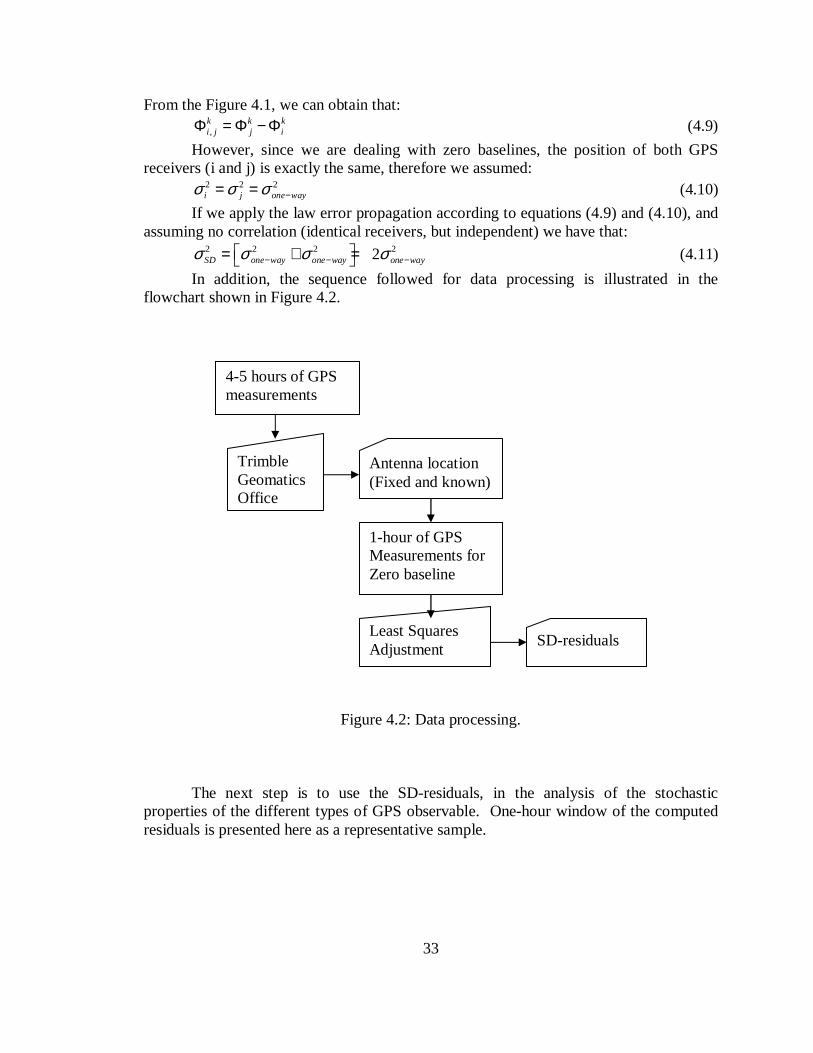
33

From the Figure 4.1, we can obtain that:

,k k ki j j iΦ = Φ − Φ (4.9)

However, since we are dealing with zero baselines, the position of both GPS receivers (i and j) is exactly the same, therefore we assumed:

2 2 2i j one wayσ σ σ −= = (4.10)

If we apply the law error propagation according to equations (4.9) and (4.10), and assuming no correlation (identical receivers, but independent) we have that:

2 2 2 22SD one way one way one wayσ σ σ σ− − − = + = (4.11)

In addition, the sequence followed for data processing is illustrated in the flowchart shown in Figure 4.2.

Figure 4.2: Data processing.

The next step is to use the SD-residuals, in the analysis of the stochastic properties of the different types of GPS observable. One-hour window of the computed residuals is presented here as a representative sample.

4-5 hours of GPS measurements

Trimble Geomatics Office

Antenna location (Fixed and known)

1-hour of GPS Measurements for Zero baseline

Least Squares Adjustment

SD-residuals

34

4.3 Test results 4.3.1. Observability plots

Figure 4.3 shows the observability plots for the different types of GPS receivers; in these plots the satellite constellation and their tracking phase (L1 and L2) is shown.

It can be observed in Figure 4.3 that, most of the satellites in view showed continuous lock during the data collection for Trimble 4000SSE for L1 and L2 carriers respectively. For Leica 9500 both satellites, PRN 21 (high) and PRN 5 (low), were observed without interruptions (continuous lock). However, Trimble 4000SSI experienced some losses for both satellites (high PRN 29 and low PRN 23) on L1 and L2 phases, which could have been caused by a loose splitter during the data collection. Also Topcon/JPS Legacy and Trimble 4700 experienced some temporary losses of lock for high and low satellites on L2 phase. However, both of the receivers maintained continuous lock for the rest of the satellites in view. Finally, Ashtech Z-S experienced some short losses of lock for PRN 17 (high), and larger losses for PRN 18 (low). Moreover, it also experienced some short losses on both L1 and L2 carrier phases for the rest of the satellites in view.

35

Figure 4.3: Observability plot on zero baseline, first row: Trimble 4000 SSE, second row: Leica 9500 and second row: Trimble 4000SSI, four row: Topcon/JPS Legacy, fifth row: Trimble 4700 with LegAnt antenna (GPS second of week 1077, 1078 and 1082). Sixth row: Ashtech Z-S, with Ashtech ground plane antenna (GPS second of week).

36

4.3.2. SD-residuals plots

As mentioned before, the least squares adjustment achieved in Section 4.2, was used to compute SD-residuals. The residuals are plotted (Figures 4.4 to 4.11) for the different types of GPS observable (L1, L2, P1 and P2) for high and low satellite respectively, for each type of receiver tested. Tables 4.2 and 4.3 summarize the results of the SD-residuals plots where the standard deviation, mean, max and min values are presented.

As can clearly be seen in Tables 4.2 and 4.3, the max and min values indicate how the SD-residuals are bounded. The variation of the mean (above or below zero) might indicate the presence of biases. However, no significant biases were discovered in the data. This indicates that the mathematical model of single difference used is capable of representing the signal, leaving only the white or random noise in the residuals. All the receivers showed residuals bounded within (5 mm) for L1 and within (15mm) for L2 on high and low satellites. Leica 9500 and Ashtech Z-S were the only receivers that showed residuals bounded within (~20 cm) for P1 on high and low satellites. In addition, Trimble 4000 was the only receiver that showed residual bounded within (2 m) on P2 for high and (3.5 m) for low satellite, the rest of the receivers showed residuals bounded within (~10 cm - ~1m). Table 4.2: Residual analysis on zero baseline, for Trimble 4000SSE (top), Leica 9500 (middle), and Trimble 4000SSI (bottom) with LegAnt antenna, (GPS second of week 1077-1078).

GPS receivers Satellite ID Standard Deviation (m)

Mean (m) Max (m) Min (m)

PRN 25 (high)

(L1) 0.0003 (L2) 0.0017 (P1) 0.1156 (P2) 0.4613

-0.0002 -0.0005 -0.0272 0.0751

0.0009 0.0058 0.4000 1.9754

-0.0014 -0.0080 -0.4601 -1.5178

4000sse

PRN 30 (low)

(L1) 0.0004 (L2) 0.0027 (P1) 0.1496 (P2) 0.7434

0.0004 0.0001 0.0095

-0.0560

0.0025 0.0168 0.5733 2.7959

-0.0014 -0.0087 -0.5904 -3.5388

PRN 21 (high)

(L1) 0.0003 (L2) 0.0014 (P1) 0.0072 (P2) 0.0252

0.00003 0.00001

-0.00128 -0.01259

0.0017 0.0063 0.0164 0.0527

-0.0018 -0.0061 -0.0669 -0.1048

Leica 9500

PRN 5 (low)

(L1) 0.0004 (L2) 0.0017 (P1) 0.0097 (P2) 0.0524

0.00002 0.00004 0.00549 0.02545

0.0019 0.0067 0.0549 0.2219

-0.0013 -0.0056 -0.0316 -0.0683

PRN 29 (high)

(L1) 0.0006 (L2) 0.0007 (P1) 0.0850 (P2) 0.1191

0.00015 -0.00005 -0.00977 -0.00874

0.0019 0.0025 0.3695 0.5248

-0.0020 -0.0026 -0.3707 -0.4441

4000SSI

PRN 23 (low)

(L1) 0.0006 (L2) 0.0008 (P1) 0.1363 (P2) 0.2076

-0.00090 -0.00090 -0.00841 -0.00838

0.0022 0.0027 0.6488 0.8901

-0.0035 -0.0046 -0.6159 -1.0735

37

Table 4.3: Residual analysis on zero baseline, for Topcon/JPS Legacy (top), Trimble 4700 (middle) with LegAnt antenna, and Ashtech Z-S (bottom) with Ashtech ground plane antenna zero baseline (GPS second of week 1082).

GPS receivers Satellite ID

Standard Deviation (m)

Mean (m) Max (m) Min (m)

PRN 29 (high)

(L1) 0.0004 (L2) 0.0005 (P1) 0.0863 (P2) 0.1040

0.00002 0.00001

-0.00370 -0.01090

0.0015 0.0019 0.2785 0.3879

-0.0017 -0.0019 -0.3128 -0.3560

Javad/Leg

PRN 5 (low)

(L1) 0.0006 (L2) 0.0009 (P1) 0.1549 (P2) 0.1937

-0.00002 -0.00004 0.00997 0.02293

0.0027 0.0036 0.5767 0.7396

-0.0022 -0.0030 -0.5257 -0.8313

PRN 29 (high)

(L1) 0.0012 (L2) 0.0021 (P1) 0.1861 (P2) 0.1828

0.00005 0.00019 0.01183

-0.00180

0.0040 0.0080 0.6543 0.6786

-0.0037 -0.0078 -0.7285 -0.6886

T4700 PRN 5 (low)

(L1) 0.0013 (L2) 0.0033 (P1) 0.2230 (P2) 0.1955

-0.00006 -0.00030

-0.00942 0.00189

0.0045 0.0122 0.9405 0.7358

-0.0057 -0.0144 -0.7920 -0.7139

PRN 17 (high)

(L1) 0.0002 (L2) 0.0003 (P1) 0.0567 (P2) 0.1989

0.0003 -0.0012 0.0067 0.0006

0.0011 0.0001 0.2197 0.7457

-0.0006 -0.0024 -0.1637 -0.7730

Ashtech

PRN 18 (low)

(L1) 0.0002 (L2) 0.0004 (P1) 0.0592 (P2) 0.2629

-0.0004 0.0021

-0.0156 -0.0015

0.0003 0.0037 0.1689 1.0259

-0.0012 0.0006 -0.2214 -0.9424

In addition, Figures 4.4 (Trimble 4000sse) and 4.5 (Leica 9500) show that low

satellite displays residuals larger by 25-60% in comparison with the high satellite. Figures 4.6 (Trimble 4000SSI), 4.7 (Topcon/JPS Legacy) and 4.8 (Trimble 4700) show that low satellite displays residuals larger by 30-100% in comparison with high satellite. Figures 4.9 and 4.10 show an example of SD-residual plots for Topcon/JPS Legacy and Trimble 4700 with Trimble Micro-centered antenna. The results obtained using Trimble Micro-centered antenna showed a little improvement in residuals (~ 10 %) for Trimble 4700 in comparison with those obtained using Leg Ant antenna. Figure 4.11 (Ashtech Z-S) show that the low satellite displays residuals larger by 10-50% in comparison with high satellite.

Figures 4.5 for Leica 9500 show the presence of some unexpected small biases and drifts on P1 and P2, as did Ashtech Z-S on L1 and L2. These unexpected small biases and drifts which may require further investigation, for this reason those results will not be counted in the subsequent stochastic analysis.

38

0 500 1000 1500 2000 2500 3000 3500

0.001

0

0.001

SD-residuals

L1 Phase

epoch [sec]

[met

ers]

0 500 1000 1500 2000 2500 3000 3500

0.005

0

0.005

SD-residuals

L2 Phase

epoch [sec]

[met

ers]

0 500 1000 1500 2000 2500 3000 3500

0.4

0.2

0

0.2

0.4

SD-residuals

P1 Pseudo-range

epoch [sec]

[met

ers]

0 500 1000 1500 2000 2500 3000 3500

1

0

1

2

SD-residuals

P2 Pseudo-range

epoch [sec]

[met

ers]

0 500 1000 1500 2000 2500 3000 3500

0.001

0

0.001

0.002

SD-residuals

L1 Phase

epoch [sec]

[met

ers]

0 500 1000 1500 2000 2500 3000 3500

0.01

0

0.01

SD-residuals

L2 Phase

epoch [sec]

[met

ers]

0 500 1000 1500 2000 2500 3000 3500

0.5

0

0.5

SD-residuals

P1 Pseudo-range

epoch [sec]

[met

ers]

0 500 1000 1500 2000 2500 3000 3500

2

0

2

SD-residuals

P2 Pseudo-range

epoch [sec]

[met

ers]

Figure 4.4: L1, L2, P1 and P2 residuals on zero baseline for high satellite (left, elev. 72-78 deg.) and low satellite (right, elev. 18-38 deg.), Trimble 4000SSE with LegAnt antenna (GPS second of week 1077).

39

0 500 1000 1500 2000 2500 3000 3500

0.001

0

0.001

SD-residuals

L1 Phase

epoch [sec]

[met

ers]

0 500 1000 1500 2000 2500 3000 3500

0.005

0

0.005

SD-residuals

L2 Phase

epoch [sec]

[met

ers]

0 500 1000 1500 2000 2500 3000 3500

0.05

0

0.05

SD residuals

P1 Pseudo-range

epoch [sec]

[met

ers]

0 500 1000 1500 2000 2500 3000 3500

0.1

0

0.1

SD residuals

P2 Pseudo-range

epoch [sec]

[met

ers]

0 500 1000 1500 2000 2500 3000 3500

0.002

0.001

0

0.001

0.002

SD-residuals

L1 Phase

epoch [sec]

[met

ers]

0 500 1000 1500 2000 2500 3000 3500

0.005

0

0.005

SD-residuals

L2 Phase

epoch [sec]

[met

ers]

0 500 1000 1500 2000 2500 3000 35000.05

0

0.05

SD-residuals

P1 Pseudo-range

epoch [sec]

[met

ers]

0 500 1000 1500 2000 2500 3000 3500

0.1

0

0.1

0.2

SD-residuals

P2 Pseudo-range

epoch [sec]

[met

ers]

Figure 4.5: L1, L2, P1 and P2 residuals on zero baseline for high satellite (left, elev. 68-86 deg.) and for low satellite (right, elev. 19-28 deg.), Leica 9500 with LegAnt antenna (GPS second of week 1078).

40

0 500 1000 1500 2000 2500 3000 3500 4000

0.002

0

0.002

SD residuals

L1 Phase

epoch [sec]

[met

ers]

0 500 1000 1500 2000 2500 3000 3500 4000

0.004

0.002

0

0.002

0.004

SD residuals

L2 Phase

epoch [sec]

[met

ers]

0 500 1000 1500 2000 2500 3000 3500 4000

0.5

0

0.5

SD residuals

P1 Pseudo-range

epoch [sec]

[met

ers]

0 500 1000 1500 2000 2500 3000 3500 4000

0.5

0

0.5

SD residuals

P2 Pseudo-range

epoch [sec]

[met

ers]

0 500 1000 1500 2000 2500 3000 3500 4000

0.002

0

0.002

SD residuals

L1 Phase

epoch [sec]

[met

ers]

0 500 1000 1500 2000 2500 3000 3500 4000

0.005

0

0.005

SD residuals

L2 Phase

epoch [sec][m

eter

s]

0 500 1000 1500 2000 2500 3000 3500 4000

0.5

0

0.5

SD residuals

P1 Pseudo-range

epoch [sec]

[met

ers]

0 500 1000 1500 2000 2500 3000 3500 4000

1

0.5

0

0.5

1

SD residuals

P2 Pseudo-range

epoch [sec]

[met

ers]

Figure 4.6: L1, L2, P1 and P2 residuals on zero baseline for high satellite (left, elev. 60-70 deg.) and low satellite (right, elev. 12-45 deg.) Trimble 4000 SSI with LegAnt antenna (GPS second of week 1078).

41

0 500 1000 1500 2000 2500 3000 3500

0.001

0

0.001

SD-residuals

L1 Phase

epoch [sec]

[met

ers]

0 500 1000 1500 2000 2500 3000 3500

0.002

0

0.002

SD-residuals

L2 Phase

epoch [sec]

[met

ers]

0 500 1000 1500 2000 2500 3000 3500

0.2

0

0.2

SD-residuals

P1 Pseudo-range

epoch [sec]

[met

ers]

0 500 1000 1500 2000 2500 3000 3500

0.4

0.2

0

0.2

0.4

SD-residuals

P2 Pseudo-range

epoch [sec]

[met

ers]

0 500 1000 1500 2000 2500 3000 3500

0.002

0

0.002

SD-residuals

L1 Phase

epoch [sec]

[met

ers]

0 500 1000 1500 2000 2500 3000 3500

0.004

0.002

0

0.002

0.004

SD-residuals

L2 Phase

epoch [sec]

[met

ers]

0 500 1000 1500 2000 2500 3000 3500

0.5

0

0.5

SD-residuals

P1 Pseudo-range

epoch [sec]

[met

ers]

0 500 1000 1500 2000 2500 3000 3500

0.5

0

0.5

SD-residuals

P2 Pseudo-range

epoch [sec]

[met

ers]

Figure 4.7: L1, L2, P1 and P2 residuals on zero baseline for high satellite (left, elev. 62-70 deg.) and for low satellite (right, elev. 22-30 deg.), Topcon/JPS Legacy with LegAnt antenna (GPS second of week 1082).

42

0 500 1000 1500 2000 2500 3000 3500

0.004

0.002

0

0.002

0.004

SD-residuals

L1 Phase

epoch [sec]

[met

ers]

0 500 1000 1500 2000 2500 3000 3500

0.005

0

0.005

SD-residuals

L2 Phase

epoch [sec]

[met

ers]

0 500 1000 1500 2000 2500 3000 3500

0.5

0

0.5

SD-residuals

P1 Pseudo-range

epoch [sec]

[met

ers]

0 500 1000 1500 2000 2500 3000 3500

0.5

0

0.5

SD-residuals

P2 Pseudo-range

epoch [sec]

[met

ers]

0 500 1000 1500 2000 2500 3000 3500

0.005

0

0.005

SD-residuals

L1 Phase

epoch [sec]

[met

ers]

0 500 1000 1500 2000 2500 3000 3500

0.01

0

0.01

SD-residuals

L2 Phase

epoch [sec]

[met

ers]

0 500 1000 1500 2000 2500 3000 35001

0.5

0

0.5

1

SD-residuals

P1 Pseudo-range

epoch [sec]

[met

ers]

0 500 1000 1500 2000 2500 3000 35001

0.5

0

0.5

1

SD-residuals

P2 Pseudo-range

epoch [sec]

[met

ers]

Figure 4.8: L1, L2, P1 and P2 residuals on zero baseline for high satellite (left, elev. 62-70 deg.) and for low satellite (right, elev. 22-27 deg.), Trimble 4700 with LegAnt antenna (GPS second of week 1082).

43

0 500 1000 1500 2000 2500 3000 3500 4000

0.002

0

0.002

SD-residuals

L1 Phase

epoch [sec]

[met

ers]

0 500 1000 1500 2000 2500 3000 3500 4000

0.002

0

0.002

SD-residuals

L2 Phase

epoch [sec]

[met

ers]

0 500 1000 1500 2000 2500 3000 3500 4000

0.2

0

0.2

SD-residuals

P1 Pseudo-range

epoch [sec]

[met

ers]

0 500 1000 1500 2000 2500 3000 3500 4000

0.4

0.2

0

0.2

0.4

SD-residuals

P2 Pseudo-range

epoch [sec]

[met

ers]

0 500 1000 1500 2000 2500 3000 3500 4000

0.002

0

0.002

SD-residuals

L1 Phase

epoch [sec]

[met

ers]

0 500 1000 1500 2000 2500 3000 3500 4000

0.004

0.002

0

0.002

0.004

SD-residuals

L2 Phase

epoch [sec]

[met

ers]

0 500 1000 1500 2000 2500 3000 3500 4000

0.5

0

0.5

SD-residuals

P1 Pseudo-range

epoch [sec]

[met

ers]

0 500 1000 1500 2000 2500 3000 3500 4000

0.5

0

0.5

SD-residuals

P2 Pseudo-range

epoch [sec]

[met

ers]

Figure 4.9: L1, L2, P1 and P2 residuals on zero baseline for high satellite (left, elev. 57-70 deg.) and for low satellite (right, elev. 20-23 deg.), Topcon/JPS Legacy with Trimble Micro-centered antenna (GPS second of week 1082).

44

0 500 1000 1500 2000 2500 3000 3500 4000 4500

0.002

0

0.002

SD-residuals

L1 Phase

epoch [sec]

[met

ers]

0 500 1000 1500 2000 2500 3000 3500 4000 45000.005

0

0.005

SD-residuals

L2 Phase

epoch [sec]

[met

ers]

0 500 1000 1500 2000 2500 3000 3500 4000 45000.5

0

0.5

SD-residuals

P1 Pseudo-range

epoch [sec]

[met

ers]

0 500 1000 1500 2000 2500 3000 3500 4000 4500

0.5

0

0.5

SD-residuals

P2 Pseudo-range

epoch [sec]

[met

ers]

0 500 1000 1500 2000 2500 3000 3500 4000 4500

0.005

0

0.005

SD-residuals

L1 Phase

epoch [sec]

[met

ers]

0 500 1000 1500 2000 2500 3000 3500 4000 4500

0.005

0

0.005

SD-residuals

L2 Phase

epoch [sec]

[met

ers]

0 500 1000 1500 2000 2500 3000 3500 4000 4500

0.5

0

0.5

SD-residuals

P1 Pseudo-range

epoch [sec]

[met

ers]

0 500 1000 1500 2000 2500 3000 3500 4000 4500

0.5

0

0.5

SD-residuals

P2 Pseudo-range

epoch [sec]

[met

ers]

Figure 4.10: L1, L2, P1 and P2 residuals on zero baseline for high satellite (left, elev. 57-71 deg.) and for low satellite (right, elev. 21-23 deg.), Trimble 4700 with Trimble Micro-centered antenna (GPS second of week 1082).

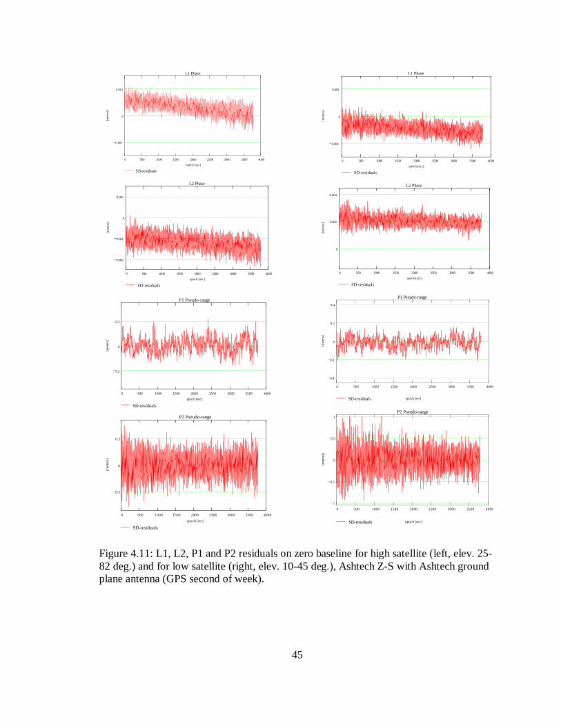
45

0 500 1000 1500 2000 2500 3000 3500 4000

0.001

0

0.001

SD-residuals

L1 Phase

epoch [sec]

[met

ers]

0 500 1000 1500 2000 2500 3000 3500 4000

0.002

0.001

0

0.001

SD-residuals

L2 Phase

epoch [sec]

[met

ers]

0 500 1000 1500 2000 2500 3000 3500 4000

0.2

0

0.2

SD-residuals

P1 Pseudo-range

epoch [sec]

[met

ers]

0 500 1000 1500 2000 2500 3000 3500 4000

0.5

0

0.5

SD-residuals

P2 Pseudo-range

epoch [sec]

[met

ers]

0 500 1000 1500 2000 2500 3000 3500 4000

0.001

0

0.001

SD-residuals

L1 Phase

epoch [sec]

[met

ers]

0 500 1000 1500 2000 2500 3000 3500 4000

0

0.002

0.004

SD-residuals

L2 Phase

epoch [sec]

[met

ers]

0 500 1000 1500 2000 2500 3000 3500 4000

0.4

0.2

0

0.2

0.4

SD-residuals

P1 Pseudo-range

epoch [sec]

[met

ers]

0 500 1000 1500 2000 2500 3000 3500 4000

1

0.5

0

0.5

1

SD-residuals

P2 Pseudo-range

epoch [sec]

[met

ers]

Figure 4.11: L1, L2, P1 and P2 residuals on zero baseline for high satellite (left, elev. 25-82 deg.) and for low satellite (right, elev. 10-45 deg.), Ashtech Z-S with Ashtech ground plane antenna (GPS second of week).

46

4.3.3 Histogram plots, based on SD-residuals

Traditionally least squares techniques (used for parameter estimation) do not consider any underlying assumption related to the noise distribution of the observables. However, in order to monitor the data quality and integrity we examined a distribution of 3000 residuals based on histograms plots. In general, and according to the assumption that observation errors in surveying are normally distributed, it can be observed in Figures 4.12–4.17 that the observation noise (i.e., SD-residuals) is essentially distributed normally (shows a normal distribution). The histogram is probably the oldest and most widely used tool to analyze data distribution. For the histogram, the range of (experimental) outcomes is divided into classes (bins) and the observed frequencies, the cell counts, are presented in a bar diagram. Histograms were plotted based on Equation (3.2), and using MathCAD functions as follows:

I. We define the data set to be analyzed (e.g., x) II. We define the size, mean, and standard deviation of the data

Size: n = length of the data (x)

Mean: 1 2( ) nx x xE x x

n

+ + += = ⋯

Standard Deviation: 2

1

1( )

1

n

x ii

x xn

σ=

= −− ∑

III. We compute the normal density( )p x , given by (3.2)

Figure 4.12 displays histograms of the SD-residuals for Trimble 4000SSE and, it shows the presence of a small bias for L1, L2, P1 and P2 (high and low satellites), respectively. Plots for all high and low satellites seem to show a uniform normal distribution of the residuals. Figure 4.13 displays histograms of the SD-residuals for Leica 9500 and, it also shows the presence of a small bias for P1 and P2 for high and low satellites, respectively. As mentioned in the previous section, some drift can be observed in the plots for P1 (high) and P2 (low) where the residuals illustrated there do not follow the normal distribution properly. Therefore results obtained for P1 and P2 are not taken into account in the stochastic analysis of this research and they may require further investigation.

Histograms of the SD-residuals for Trimble 4000SSI, Javad Legacy and Trimble 4700 are shown in Figures 4.14, 4.15 and 4.16. Those experienced the presence of a very small bias for P1 and P2 (high and low satellites), respectively. Here, all the plots showed a normal distribution of the residuals for the different types of observables. Figure 4.17 displays histograms of the SD-residuals for Ashtech Z-S and, it shows the presence of a small bias for L1, L2, P1 and P2 (high and low satellites), respectively. Plots for the carrier phases (high and low satellites) showed also some drift (refer to previous section), and all the residuals showed a normal distribution. Similar as for Leica 9500, the results obtained for L1 and L2 are not consider in the stochastic analysis of this research, and they may require further investigation. In general, for all the GPS receivers most of the plots follow a normal distribution, except for: P1 (high) and P2 (low) for Leica.

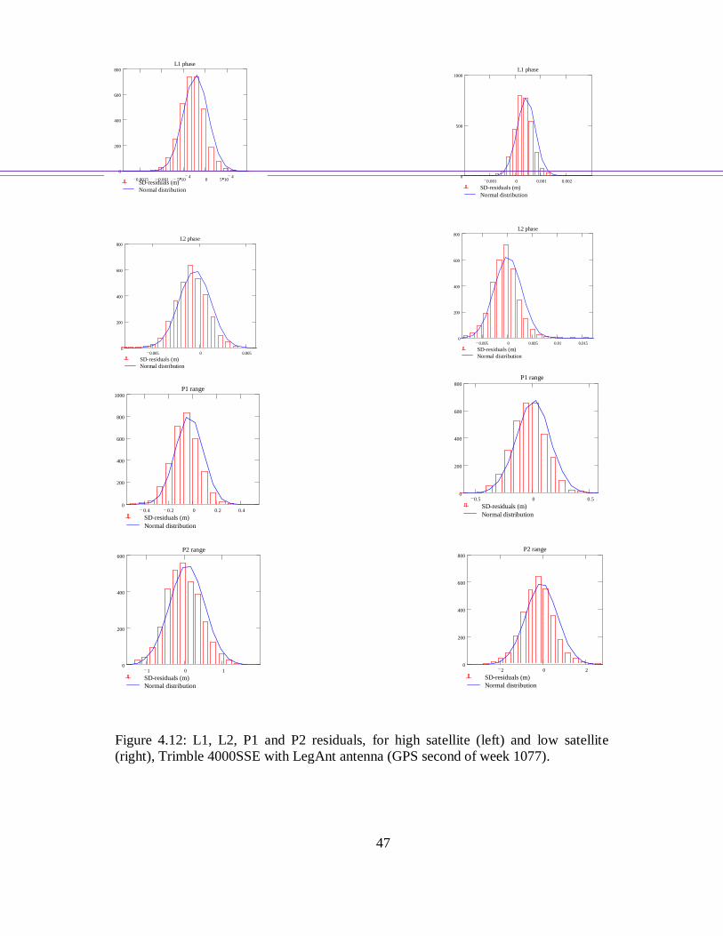
47

0.001 0 0.001 0.0020

500

1000

SD-residuals (m) Normal distribution

L1 phase

0.005 0 0.0050

200

400

600

800

SD-residuals (m) Normal distribution

L2 phase

0.005 0 0.005 0.01 0.0150

200

400

600

800

SD-residuals (m) Normal distribution

L2 phase

0.4 0.2 0 0.2 0.40

200

400

600

800

1000

SD-residuals (m) Normal distribution

P1 range

0.5 0 0.50

200

400

600

800

SD-residuals (m) Normal distribution

P1 range

1 0 10

200

400

600

SD-residuals (m) Normal distribution

P2 range

2 0 20

200

400

600

800

SD-residuals (m)Normal distribution

P2 range

Figure 4.12: L1, L2, P1 and P2 residuals, for high satellite (left) and low satellite (right), Trimble 4000SSE with LegAnt antenna (GPS second of week 1077).

0.0015 0.001 5 104

0 5 104

0

200

400

600

800

SD-residuals (m) Normal distribution

L1 phase

48

0.001 0 0.0010

200

400

600

800

1000

SD-residuals (m)Normal distribution

L1 phase

0.001 0 0.0010

200

400

600

800

1000

SD-residuals (m)Normal distribution

L1 phase

0.006 0.004 0.002 0 0.002 0.004 0.0060

200

400

600

800

SD-residuals (m)Normal distribution

L2 phase

0.004 0.002 0 0.002 0.004 0.0060

200

400

600

SD-residuals (m)Normal distribution

L2 phase

0.02 0.01 0 0.010

200

400

600

800

SD-residuals (m)Normal distribution

P1 range

0.02 0 0.02 0.040

200

400

600

800

SD-residuals (m)Normal distribution

P1 range

0.06 0.04 0.02 0 0.02 0.04 0.060

200

400

600

SD-residuals (m)Normal distribution

P2 range

0.1 0.05 0 0.05 0.1 0.150

200

400

600

SD-residuals (m)Normal distribution

P2 range

Figure 4.13: L1, L2, P1 and P2 residuals, for high satellite (left) and low satellite (right), Leica 9500 with LegAnt antenna (GPS second of week 1078).

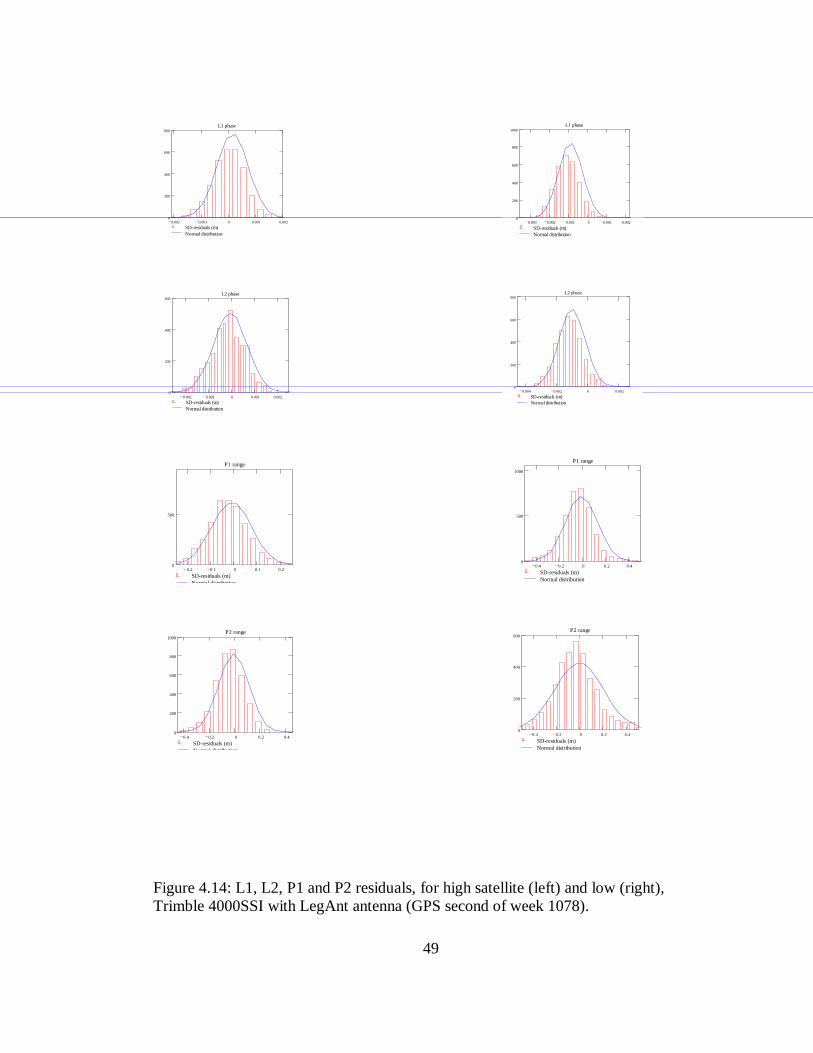
49

0.002 0.001 0 0.001 0.0020

200

400

600

800

SD-residuals (m)Normal distribution

L1 phase

0.003 0.002 0.001 0 0.001 0.0020

200

400

600

800

1000

SD-residuals (m)Normal distribution

L1 phase

0.002 0.001 0 0.001 0.0020

200

400

600

SD-residuals (m)Normal distribution

L2 phase

0.004 0.002 0 0.0020

200

400

600

800

SD-residuals (m)Normal distribution

L2 phase

0.2 0.1 0 0.1 0.20

500

SD-residuals (m)Normal distribution

P1 range

0.4 0.2 0 0.2 0.40

500

1000

SD-residuals (m)Normal distribution

P1 range

0.4 0.2 0 0.2 0.40

200

400

600

800

1000

SD-residuals (m)Normal distribution

P2 range

0.4 0.2 0 0.2 0.40

200

400

600

SD-residuals (m)Normal distribution

P2 range

Figure 4.14: L1, L2, P1 and P2 residuals, for high satellite (left) and low (right), Trimble 4000SSI with LegAnt antenna (GPS second of week 1078).

50

0.001 0 0.0010

200

400

600

800

1000

SD-residuals (m)Normal distribution

L1 phase

0.002 0.001 0 0.001 0.0020

200

400

600

800

SD-residuals (m)Normal distribution

L1phase

0.001 0 0.0010

200

400

600

800

SD-residuals (m)Normal distribution

L2 phase

0.002 0 0.0020

200

400

600

SD-residuals (m)Normal distribution

L2 phase

0.2 0.1 0 0.1 0.20

200

400

600

800

SD-residuals (m)Normal distribution

P1 range

0.4 0.2 0 0.2 0.40

200

400

600

SD-residuals (m)Normal distribution

P1 range

0.2 0 0.20

200

400

600

SD-residuals (m)Normal distribution

P2 range

0.4 0.2 0 0.2 0.40

200

400

600

SD-residuals (m)Normal distribution

P2 range

Figure 4.15: L1, L2, P1 and P2 residuals, for high satellite (left) and low satellite (right), Topcon/JPS Legacy with LegAnt antenna (GPS second of week 1082).

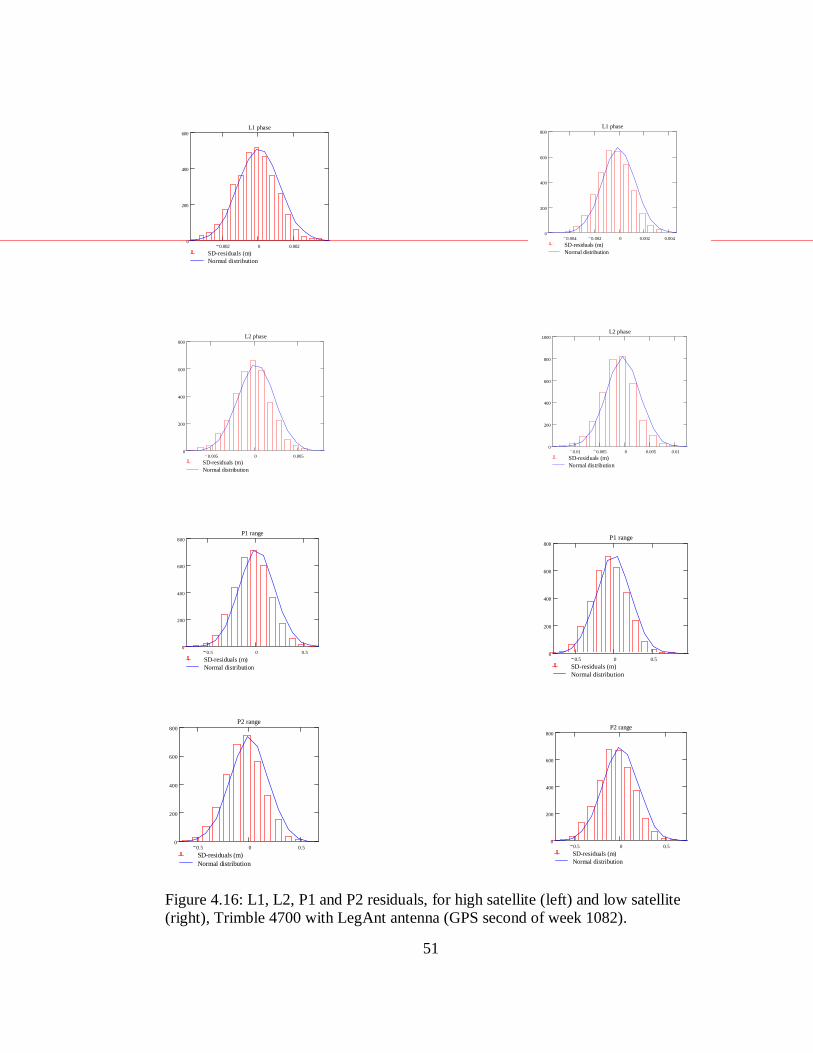
51

0.5 0 0.50

200

400

600

800

SD-residuals (m)Normal distribution

P2 range

0.5 0 0.50

200

400

600

800

SD-residuals (m)Normal distribution

P2 range

0.002 0 0.0020

200

400

600

SD-residuals (m)Normal distribution

L1 phase

0.004 0.002 0 0.002 0.0040

200

400

600

800

SD-residuals (m)Normal distribution

L1 phase

0.005 0 0.0050

200

400

600

800

SD-residuals (m)Normal distribution

L2 phase

0.01 0.005 0 0.005 0.010

200

400

600

800

1000

SD-residuals (m)Normal distribution

L2 phase

0.5 0 0.50

200

400

600

800

SD-residuals (m)Normal distribution

P1 range

0.5 0 0.50

200

400

600

800

SD-residuals (m)Normal distribution

P1 range

Figure 4.16: L1, L2, P1 and P2 residuals, for high satellite (left) and low satellite (right), Trimble 4700 with LegAnt antenna (GPS second of week 1082).

52

5 104

0 5 104

0.001

0

200

400

600

800

1000

SD-residuals (m) Normal distribution

L1 phase

0.001 5 104

0

0

200

400

600

800

1000

SD-residuals (m) Normal distribution

L1 phase

0.002 0.0015 0.001 5 104

0

0

200

400

600

800

1000

SD-residuals (m) Normal distribution

L2 phase

0 0.001 0.002 0.0030

500

1000

1500

SD-residuals (m) Normal distribution

L2 phase

0.1 0 0.10

500

1000

SD-residuals (m) Normal distribution

P1 range

0.1 0 0.10

500

1000

SD-residuals (m) Normal distribution

P1 range

0.4 0.2 0 0.2 0.40

200

400

600

SD-residuals (m) Normal distribution

P2 range

0.5 0 0.50

200

400

600

800

SD-residuals (m) Normal distribution

P2 range

Figure 4.17: L1, L2, P1 and P2 residuals, for high satellite (left) and low satellite (right), Ashtech Z-S with Ashtech ground plane antenna (GPS second of week).

53

4.3.4 Power Spectral Density (PSD) plots based on SD-residuals

PSD was computed in order to determine the correlation of the residuals at different frequencies. The computations needed to create these plots were made based on the following equation, previously denoted as (3.4), since as mentioned before (refer Section 3.6.3) the spectrum of the autocorrelation function is the Power Spectral Density (PSD) function.

*1( ) ( ) ( )gg k T k T kG G

N tΦ =

⋅ ∆⌢

ɶ ɶ

where N, t∆ and *( )T kGɶ were defined before.

Figure 4.18 shows that low and high frequency spectral components have the same contribution to the correlation of the residuals for Trimble 4000SSE on L1 and P1 for PRN 25 (high) and PRN 30 (low). In contrast, plots for L2 and P2 (high and low satellites) show that only the low frequency spectral components contribute to the correlation of the residuals.

Figure 4.19 shows that low and high frequency spectral components have the same contribution to the correlation of the residuals for Leica 9500 on L1 and L2 for PRN 21 (high) and PRN 5 (low). Low frequency spectral components seem to contribute only for P1 and P2 (high and low satellites).

Figures 4.20 and 4.21 show that for Trimble 4000SSI and Topcon/JPS Legacy low and high frequency spectral components have similar influence on L1 for high and lows, respectively; however, for the rest of the plots (L2, P1 and P2) only low frequency spectral components contribute to the correlation of the residuals.

Figure 4.22 shows that both low and high frequency spectral components have the same contribution to the correlation of the residuals for Trimble 4700 on L1, L2, P1 and P2 for PRN 29 (high) and PRN 5 (low).

Figure 4.23 shows that only low frequency spectral components have contribution to the correlation of the residuals, for Ashtech Z-S on P1 for PRN 17 (high) and PRN 18 (low). On the other hand, both frequency spectral components (low and high) have similar contribution to the correlation of the residuals for L1, L2 and P2 for high and low satellites, respectively.

In general, all the receivers showed that the low and high frequency spectral components have similar contribution to the correlation of the residuals for L1 (high and low satellites). Plots for Trimble 4700 indicate that both low and high frequency spectral components contributed to the correlation of the residuals for all the observables (high and low satellites). The rest of the plots indicate that for some receivers the low and high frequency spectral components contribute together to the correlation of the residuals, and sometimes only the low frequency spectral components. The observed differences among the receivers most probably follow from the different codeless or semi-codeless techniques implemented to recover L2/P2.

54

500 1000 15000

5

PSD [cy/s]

P1 range

epoch [sec]

500 1000 15000

5

10

PSD [cy/s]

P1 range

epoch [sec]

500 1000 15000

20

40

60

PSD [cy/s]

P2 range

epoch [sec]

500 1000 15000

20

40

60

PSD [cy/s]

P2 range

epoch [sec]

Figure 4.18: Power Spectral Density for L1, L2, P1 and P2 residuals, for high satellite (left) and low satellite (right), Trimble 4000SSE with LegAnt antenna (GPS second of week 1077).

500 1000 15000

5

10

PSD [cy/s]

L1 phase

epoch [sec]

500 1000 15000

20

40

PSD [cy/s]

L2 phase

epoch [sec]

500 1000 15000

2

4

PSD [cy/s]

L1 phase

epoch [sec]

500 1000 15000

20

40

PSD [cy/s]

L2 phase

epoch [sec]

55

500 1000 15000

5

PSD [cy/s]

L1 phase

epoch [sec]

500 1000 15000

5

PSD [cy/s]

L1 phase

epoch [sec]

500 1000 15000

5

10

PSD [cy/s]

L2 phase

epoch [sec]

500 1000 15000

5

PSD [cy/s]

L2 phase

epoch [sec]

Figure 4.19: Power Spectral Density for L1 and L2 residuals, for high satellite (left) and low (right), Leica 9500 with LegAnt antenna (GPS second of week 1078).

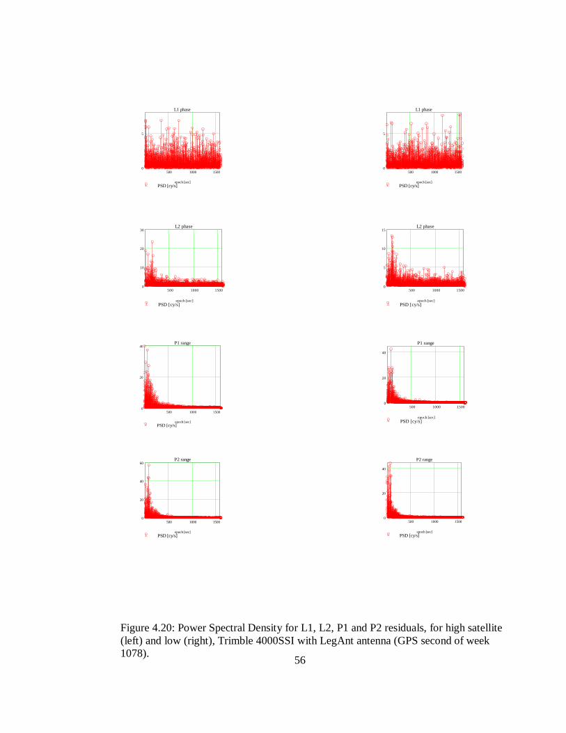
56

500 1000 15000

5

PSD [cy/s]

L1 phase

epoch [sec]

500 1000 15000

5

PSD [cy/s]

L1 phase

epoch [sec]

500 1000 15000

10

20

30

PSD [cy/s]

L2 phase

epoch [sec]

500 1000 15000

5

10

15

PSD [cy/s]

L2 phase

epoch [sec]

500 1000 15000

20

40

PSD [cy/s]

P1 range

epoch [sec]

500 1000 15000

20

40

PSD [cy/s]

P1 range

epoch [sec]

500 1000 15000

20

40

60

PSD [cy/s]

P2 range

epoch [sec]

500 1000 15000

20

40

PSD [cy/s]

P2 range

epoch [sec]

Figure 4.20: Power Spectral Density for L1, L2, P1 and P2 residuals, for high satellite (left) and low (right), Trimble 4000SSI with LegAnt antenna (GPS second of week 1078).

57

500 1000 15000

10

20

30

PSD [cy/s]

P2 range

epoch [sec]

500 1000 15000

20

40

PSD [cy/s]

P2 range

epoch [sec]

500 1000 15000

5

10

PSD [cy/s]

L1 phase

epoch [sec]

500 1000 15000

5

10

PSD [cy/s]

L1 phase

epoch [sec]

500 1000 15000

10

20

PSD [cy/s]

L2 phase

epoch [sec]

500 1000 15000

10

20

PSD [cy/s]

L2 phase

epoch [sec]

500 1000 15000

10

20

30

PSD [cy/s]

P1 range

epoch [sec]

500 1000 15000

20

40

PSD [cy/s]

P1 range

epoch [sec]

Figure 4.21: Power Spectral Density for L1, L2, P1 and P2 residuals, for high satellite (left) and low satellite (right), Topcon/JPS Legacy with LegAnt antenna (GPS second of week 1082).

58

500 1000 15000

5

10

PSD [cy/s]

P2 range

epoch [sec]

500 1000 15000

10

20

PSD [cy/s]

P2 range

epoch [sec]

500 1000 15000

5

10

PSD [cy/s]

L1 phase

epoch [sec]

500 1000 15000

5

10

PSD [cy/s]

L1 phase

epoch [sec]

500 1000 15000

5

10

PSD [cy/s]

L2 phase

epoch [sec]

500 1000 15000

5

10

PSD [cy/s]

L2 phase

epoch [sec]

500 1000 15000

5

10

PSD [cy/s]

P1 range

epoch [sec]

500 1000 15000

5

PSD [cy/s]

P1 range

epoch [sec]

Figure 4.22: Power Spectral Density for L1, L2, P1 and P2 residuals, for high satellite (left) and low satellite (right), Trimble 4700 with LegAnt antenna (GPS second of week 1082).

59

500 1000 15000

50

PSD [cy/s]

P1 range

epoch [sec]

500 1000 15000

50

PSD [cy/s]

P1 range

epoch [sec]

500 1000 15000

5

10

PSD [cy/s]

P2 range

epoch [sec]

500 1000 15000

5

10

PSD [cy/s]

P2 range

epoch [sec]

Figure 4.23: Power Spectral Density for P1 and P2 residuals on zero baseline for high satellite (left, elev. 25-82 deg.) and for low satellite (right, elev. 10-45 deg.), Ashtech Z-S with Ashtech ground plane antenna (GPS second of week).

60

4.3.5 Normalized Autocorrelation (correlogram plots) based on SD-residuals

The normalized autocorrelation plots were computed in order to verify if the different types of GPS observables contain only white noise (i.e., that they are not correlated from epoch to epoch). The computations needed to create the normalized autocorrelation plots are described below:

As mentioned in Section 3.6.3, Equation 3.4 (given below) represents the spectrum of the autocorrelation, which can be obtained by a simple multiplication of the normalized function with its complex conjugate in the frequency domain.

*1( ) ( ) ( )gg k T k T kG G

N tΦ =

⋅ ∆⌢

ɶ ɶ

The inverse of the Fourier transform of the above equation results in the autocorrelation in the space domain, that is:

1( )gg kF autocorrelation− Φ =⌢

Then, the computed autocorrelation is normalized by dividing it by its value at zero lag. By definition, normalizing the autocorrelation leads to its value equal to 1 at zero lag. The plot of the normailized autocorrelation is called correlogram. In other words, the normalized autocorrelation portrays the autocorrelation coefficient versus the time lag (time interval between two samples). The time interval ( cτ ), at which the process

may be considered decorrelated is defined by 1

( ) (0)2cR Rτ = (Moritz, 1980); in our case

(0) 1R = (at zero lag); therefore, 1

( )2cR τ = .

In order to summarize the results of the autocorrelation analysis, the correlation time was divided into two classes following classification proposed by (Bona et al. 2000b): (1) short correlation times ( 5≤ seconds), and (2) large correlation times (>5 seconds). Table 4.4 shows the correlation time for the different types of GPS observables for high and low satellites, respectively. The empty cells refer to the GPS observables that require further investigation (refer to Sections 4.3.2 and 4.3.3).

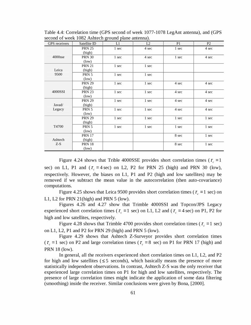
61

Table 4.4: Correlation time (GPS second of week 1077-1078 LegAnt antenna), and (GPS second of week 1082 Ashtech ground plane antenna).

GPS receivers Satellite ID L1 L2 P1 P2 PRN 25 (high)

1 sec 4 sec 1 sec 4 sec

4000sse

PRN 30 (low)

1 sec 4 sec 1 sec 4 sec

PRN 21 (high)

1 sec 1 sec Leica 9500

PRN 5 (low)

1 sec 1 sec

PRN 29 (high)

1 sec 1 sec 4 sec 4 sec

4000SSI

PRN 23 (low)

1 sec 1 sec 4 sec 4 sec

PRN 29 (high)

1 sec 1 sec 4 sec 4 sec Javad/ Legacy

PRN 5 (low)

1 sec 1 sec 4 sec 4 sec

PRN 29 (high)

1 sec 1 sec 1 sec 1 sec

T4700 PRN 5 (low)

1 sec 1 sec 1 sec 1 sec

PRN 17 (high)

8 sec 1 sec Ashtech

Z-S

PRN 18 (low)

8 sec 1 sec

Figure 4.24 shows that Trible 4000SSE provides short correlation times ( 1cτ =

sec) on L1, P1 and ( 4cτ = sec) on L2, P2 for PRN 25 (high) and PRN 30 (low),

respectively. However, the biases on L1, P1 and P2 (high and low satellites) may be removed if we subtract the mean value in the autocorrelation (then auto-covariance) computations.

Figure 4.25 shows that Leica 9500 provides short correlation times ( 1cτ = sec) on

L1, L2 for PRN 21(high) and PRN 5 (low). Figures 4.26 and 4.27 show that Trimble 4000SSI and Topcon/JPS Legacy

experienced short correlation times ( 1cτ = sec) on L1, L2 and ( 4cτ = sec) on P1, P2 for

high and low satellites, respectively. Figure 4.28 shows that Trimble 4700 provides short correlation times ( 1cτ = sec)

on L1, L2, P1 and P2 for PRN 29 (high) and PRN 5 (low). Figure 4.29 shows that Ashtech Z-Surveyor provides short correlation times

( 1cτ = sec) on P2 and large correlation times ( 8cτ = sec) on P1 for PRN 17 (high) and

PRN 18 (low). In general, all the receivers experienced short correlation times on L1, L2, and P2

for high and low satellites ( 5≤ seconds), which basically means the presence of more statistically independent observations. In contrast, Ashtech Z-S was the only receiver that experienced large correlation times on P1 for high and low satellites, respectively. The presence of large correlation times might indicate the application of some data filtering (smoothing) inside the receiver. Similar conclusions were given by Bona, [2000].

62

0 5 10 15 20

0.5

0.5

1

autocorrelation

L1 phase

Time [sec]

Figure 4.24: Correlograms for L1, L2, P1 and P2 residuals, for high satellite (left) and low satellite (right), Trimble 4000SSE with LegAnt antenna (GPS second of week 1077).

0 5 10 15 20

0.5

0.5

1

autocorrelation

P1 range

Time [sec]

0 5 10 15 20

0.5

0.5

1

autocorrelation

P2 range

Time [sec]

0 5 10 15 20

0.5

0.5

1

autocorrelation

L1 phase

Time [sec]

0 5 10 15 20

0.5

0.5

1

autocorrelation

P2 range

Time [sec]

n

0 5 10 15 20

0.5

0.5

1

autocorrelation

L2 phase

Time [sec]

0 5 10 15 20

0.5

0.5

1

autocorrelation

L2 phase

Time [sec]

0 5 10 15 20

0.5

0.5

1

autocorrelation

P1 range

Time [sec]

63

0 5 10 15 20

0.5

0.5

1

autocorrelation

L1 phase

Time [sec]

0 5 10 15 20

0.5

0.5

1

autocorrelation

L1 phase

Time [sec]

0 5 10 15 20

0.5

0.5

1

autocorrelation

L2 phase

Time [sec]

Figure 4.25: Correlograms for L1 and L2 residuals, for high satellite (left) and low satellite (right), Leica 9500 with LegAnt antenna (GPS second of week 1078).

0 5 10 15 20

0.5

0.5

1

autocorrelation

L2 phase

Time [sec]

64

0 5 10 15 20

0.5

1

autocorrelation

L1 phase

Time [sec]

0 5 10 15 20

0.5

0.5

1

autocorrelation

P1 range

Time [sec]

0 5 10 15 20

0.5

0.5

1

autocorrelation

P2 range

Time [sec]

0 5 10 15 20

0.5

0.5

1

autocorrelation

L2 phase

Time [sec]

Figure 4.26: Correlograms for L1, L2, P1 and P2 residuals, for high satellite (left) and low satellite (right), Trimble 4000SSI with LegAnt antenna (GPS second of week 1078).

0 5 10 15 20

0.5

0.5

1

autocorrelation

L2 phase

Time [sec]

0 5 10 15 20

0.5

0.5

1

autocorrelation

P1 range

Time [sec]

0 5 10 15 20

0.5

0.5

1

autocorrelation

P2 range

Time [sec]

0 5 10 15 20

0.5

0.5

1

autocorrelation

L1 phase

Time [sec]

65

0 5 10 15 20

0.5

0.5

1

autocorrelation

P2 range

Time [sec]

0 5 10 15 20

0.5

0.5

1

autocorrelation

P2 range

Time [sec]

0 10 20 30

0.5

1

autocorrelation

L1 phase

Time [sec]

0 5 10 15 20

0.5

0.5

1

autocorrelation

L1 phase

Time [sec]

0 5 10 15 20

0.5

0.5

1

autocorrelation

L2 phase

Time [sec]

0 5 10 15 20

0.5

0.5

1

autocorrelation

L2 phase

Time [sec]

0 5 10 15 20

0.5

0.5

1

autocorrelation

P1 range

Time [sec]

0 5 10 15 20

0.5

0.5

1

autocorrelation

P1 range

Time [sec]

Figure 4.27: Correlograms for L1, L2, P1 and P2 residuals, PRN 29 (left) and PRN 5 (right), Topcon/JPS Legacy with LegAnt antenna (GPS second of week 1082).

66

0 5 10 15 20

0.5

0.5

1

autocorrelation

L1 phase

Time [sec]

0 5 10 15 20

0.5

0.5

1

autocorrelation

L1 phase

Time [sec]

0 5 10 15 20

0.5

0.5

1

autocorrelation

L2 phase

Time [sec]

0 5 10 15 20

0.5

0.5

1

autocorrelation

L2 phase

Time [sec]

0 5 10 15 20

0.5

0.5

1

autocorrelation

P1 range

Time [sec]

0 5 10 15 20

0.5

0.5

1

autocorrelation

P1 range

Time [sec]

n

0 5 10 15 20

0.5

0.5

1

autocorrelation

P2 range

Time [sec]

0 10 20 30 40

0.5

0.5

1

autocorrelation

P2 range

Time [sec]

Figure 4.28: Correlograms for L1, L2, P1 and P2 residuals, PRN 29 (left) and PRN 5 (right), Trimble 4700 with LegAnt antenna (GPS second of week 1082).

67

0 5 10 15 20

0.5

1

autocorrelation

P1 range

Time [sec]

0 5 10 15 20

0.5

0.5

1

autocorrelation

P1 range

Time [sec]

0 5 10 15 20

0.5

0.5

1

autocorrelation

P2 range

Time [sec]

0 5 10 15 20

0.5

0.5

1

autocorrelation

P2 range

Time [sec]

Figure 4.29: Correlograms for P1 and P2 residuals, for high satellite (left) and low satellite (right), Ashtech Z-S with Ashtech ground plane antenna (GPS second of week).

68

4.3.6 Cross-correlation function and cross-correlation coefficient

The cross-correlation function was computed based on SD-residuals, in order to

determine the correlation among the different types of GPS observables as follows: As mentioned in Section 3.6.3, Equation 3.4 (given below) represents the

spectrum of the auto/cross-correlation. *1

( ) ( ) ( )gh k T k T kG HN t

Φ =⋅ ∆

⌢ɶ ɶ

The inverse of the Fourier transform of the above equation results in the cross-correlation in the space domain, that is:

1( )gh kF cross correlation− Φ = −⌢

The results obtained from the auto and cross-correlation functions (derived from the stochastic analysis) will be used to construct the alternative variance-covariance matrix, in order to test its impact in positioning estimators (refer to Chapter 6).

On the other hand, the cross-correlation coefficient was computed based on one-way residuals, in order to determine the amount of correlation between the GPS observable (L1, L2, P1 and P2) as shown below:

It is well known that for two sets of random series 1 2, ,....., nx x x and 1 2, ,....., ny y y ,

their variances are given by the well-known formulas:

2 2

1

1( )

1

n

x ii

x xn

σ=

= −− ∑

and

2 2

1

1( )

1

n

y ii

y yn

σ=

= −− ∑

And their covariance

,1

1( )( )

1

n

x y i ii

x x y yn

σ=

= − −− ∑

where:

x and y - the mean values for each random series. Then, the correlation coefficient between the two random series is given by:

,, 2 2

x yx y

x y

σρ

σ σ=

⋅

Table 4.5 summarizes the cross-correlation coefficients for one-way GPS observables (high and low satellites). As can be seen in Table 4.5, high and low satellites show a small cross correlation between L1P1, L1P2, L2P1 and L2 P2 (of the order of 1-7 %), except between L1L2 or P1P2, where larger cross-correlation is observed. The GPS receivers that showed high levels of cross correlation between phases for high and low satellites were: Trimble 4000SSI (35-37 %), Topcon/JPS Legacy (30-33 %) and Ashtech Z-surveyor (25-32 %). In contrast, Leica 9500 showed high correlation (33 %) between pseudo-ranges for low satellite only. From the experiments, the carrier phases always show a positive cross-correlation, as did the pseudo-ranges. This basically means that,

69

both signals experienced the same behavior or tendency. In general the cross correlation coefficients obtained from all the GPS receivers seem to be consistent with the results provided in Bona [2000]. Table 4.5: Cross correlation coefficient between L1, L2, P1 and P2 (one-way residuals), for high and low, first row: Trimble 4000SSE, second row: Leica 9500, third row: Trimble 4000SSI, fourth row: Topcon/JPS Legacy, fifth row: Trimble 4700 with LegAnt antenna, (GPS second of week 1077, 1078 and 1082), sixth row: Ashtech Z-S with Ashtech ground plane antenna, (GPS second of week).

Cross-correlation coefficient GPS receivers

Satellite ID

rL1L2 rL1P1 rL1P2 rL2P1 rL2P2 rP1P2

PRN 25 (high)

0.06 -0.01 0.00 0.00 0.01 0.13 T4000SSE

PRN 30 (low)

0.05 0.00 -0.02 0.02 -0.01 0.11

PRN 21 (high)

0.10 0.01 -0.01 -0.01 0.03 0.08 Leica 9500

PRN 5 (low)

0.08 0.02 -0.01 0.00 0.02 0.33

PRN 29 (high)

0.37 0.03 -0.01 0.03 0.05 0.02 T4000SSI

PRN 23

(low) 0.35 0.02 -0.01 0.04 0.07 0.03

PRN 29 (high)

0.30 0.01 0.01 -0.01 0.01 0.03 Topcon

JPS/Legac

PRN 5 (low)

0.33 0.01 0.01 -0.01 0.00 0.03

PRN 29 (high)

0.24 0.00 0.00 0.00 0.00 0.06 T-4700

PRN 5 (low)

0.16 0.00 0.00 0.00 0.00 0.06

PRN 17 (high)

0.32 0.00 -0.01 -0.02 0.01 0.00 Ashtech Z-S

PRN 18 (low)

0.25 0.00 -0.01 -0.03 0.01 0.00

70

CHAPTER 5

AN EXAMPLE OF SHORT BASELINE RESULTS

5.1 An Example of GPS Survey Analysis and Results for 10-m Baseline

As mentioned in chapter four, only zero baseline results are analyzed in detail here, since zero baseline scenario is suitable for analyzing the residuals which may contain only the remaining receiver noise, as explained earlier. Our primary goal is to analyze the noise characteristics of 6 GPS receivers and the stochastic properties of GPS observables. However, under the assumption that only the receiver’s noise is the primary component of the zero baseline measurements, the 10-meters baseline results, which are presented as an example may illustrate a more real scenario of the common receiver performance. 5.2 The 10-m GPS Static Surveys

The GPS static surveys presented for the 10-m baselines were performed on three different dates: August 27, September 03 and October 01, 2000, on a test range established at OSU West Campus (Figure 5.1). There were no obstructions within 100 meters of the survey, except some light poles, which could cause some multipath effects.

Again, Trimble Geomatics Office software was used to process the data collected. Some of the main specifications for the GPS surveys were: elevation mask 10 degrees and 1-second time interval. The antennas on the 10-meters baseline were placed on 2-meter fixed tripods.

The GPS static surveys presented here comprise five 10-meter baselines (see Figure 5.1).

71

Figure 5.1: GPS receiver configuration for 10-m baseline measurements.

Figures 5.2 to 5.7 show examples of SD-residuals obtained for L1, L2, P1, and P2 for the GPS receivers tested on 10-m baseline. It can be observed in Figure 5.2 that, Topcon/JPS Legacy experiences residuals bounded within (7 mm) on L1, and within (11 mm) on L2 for PRN 29 (high) and PRN 5 (low), respectively. Plots for P1 and P2 show residuals bounded within (1-2 m) for high satellite and within (2-2.3 m) for low satellite.

Figure 5.3 indicates that Leica 9500 shows residuals bounded within (5 to 10 mm) on L1 and L2, and within (10 to 20 cm) on P1 and P2 for PRN 21 (high) and PRN 5 (low), respectively. A very pronounced bias (~5 cm) is also seen in the plots for P1 and P2. Drifts can again be observed on L1 and L2 for high and low satellite.

Figure 5.4 show that Ashtech Z-S provides residuals bounded within (12 mm) on L1, L2 for PRN17 (high), within (7 mm) on L1, L2 for PRN 18 (low) and within (1.4 m) for P1 and P2 (high and low), respectively. Similarly as Leica 9500, Ashtech Z-S experiences the presence of bias (~5-10 mm) and drift on L1 and L2 for low and high satellites.

Figure 5.5 indicates the Trimble 4000SSE provides residuals bounded within (3 mm) on L1, and within (5 mm) on L2 for PRN 25 (high) and PRN 30 (low), respectively. Plots for P1 and P2 show residuals bounded within (1.4 m) for high and low satellites. A small bias (~1-3 mm) can be seen in the plots for L1 and L2, and a bigger one (~25 cm) on P1 for high and low satellites.

T-4000SSE 10 m

10 m

T-4000SSE

T-4000SSI T-4000SSI

T/JPS Legacy T/JPS Legacy

Ashtech Z12and T-4700

Leica 9500

Leica 9500

Ashtech Z12 and T-4700

0 10

1 11

2 12

3 13

4 14

N

72

Figure 5.6 show that Trimble 4000SSI experienced residuals bounded within (6 mm) on L1 and L2, within (55 cm) on P1, and within (1.4 m) on P2 for PRN 29 (high) and PRN 23 (low), respectively. The presence of bias (1mm) for carriers, (10 cm) for pseudo-ranges can also be observed.

Figure 5.7 indicates that Trimble 4700 provides residuals bounded within (5-11 mm) on L1 and L2, and within (1.2 m) on P1 and P2 for PRN 29 (high) and PRN 5 (low), respectively. A bias (2 mm) can be seen in the plots for L1 and L2, and a bigger one (5 cm) for P1 and P2 plots.

The existence of biases, and in some cases the presence of a possible drift is the tendency in most of the plots for short baseline results, which may indicate the presence of some systematic effects (multipath and atmosphere). In addition, the results also show that for most of the SD-residuals (L1, L2, P1, and P2) the low satellites display residuals considerably bigger in comparison with the high satellites.

It is important to point out here that the example showed (figures 5.2 to 5.7), clearly indicate that the results obtained for the GPS static surveys (considering all the GPS receivers) for short baseline measurements (10-m baseline) present some considerable biases in comparison with the results obtained on zero baseline. This could be attributed to the fact that short baseline include some systematic effects not present on zero baseline measurements, used to estimate the receiver noise.

73

0 500 1000 1500 2000 2500 3000 3500 4000

0.005

0

0.005

SD-residuals

L1 Phase

epoch [sec]

[me

ters

]

0 500 1000 1500 2000 2500 3000 3500 4000

0.01

0

0.01

SD-residuals

L1 Phase

epoch [sec]

[me

ters

]

0 500 1000 1500 2000 2500 3000 3500 4000

0.005

0

0.005

0.01

SD-residuals

L2 Phase

epoch [sec]

[met

ers]

0 500 1000 1500 2000 2500 3000 3500 4000

2

1

0

1

SD-residuals

P1 Pseudo-range

epoch [sec]

[me

ters

]

0 500 1000 1500 2000 2500 3000 3500 4000

1

0

1

SD-residuals

P2 Pseudo-range

epoch [sec]

[met

ers]

0 500 1000 1500 2000 2500 3000 3500 4000

0.01

0

0.01

SD-residuals

L2 Phase

epoch [sec]

[me

ters

]

0 500 1000 1500 2000 2500 3000 3500 40002

1

0

1

2

SD-residuals

P1 Pseudo-range

epoch [sec]

[me

ters

]

0 500 1000 1500 2000 2500 3000 3500 4000

2

0

2

SD-residuals

P2 Pseudo-range

epoch [sec]

[me

ters

]

Figure 5.2: L1, L2, P1 and P2 residuals on 10-m baseline for high satellite (left, elev. 20-70 deg.) and low satellite (right, elev. 10-18 deg.), Topcon/JPS Legacy (GPS second of week 1077).

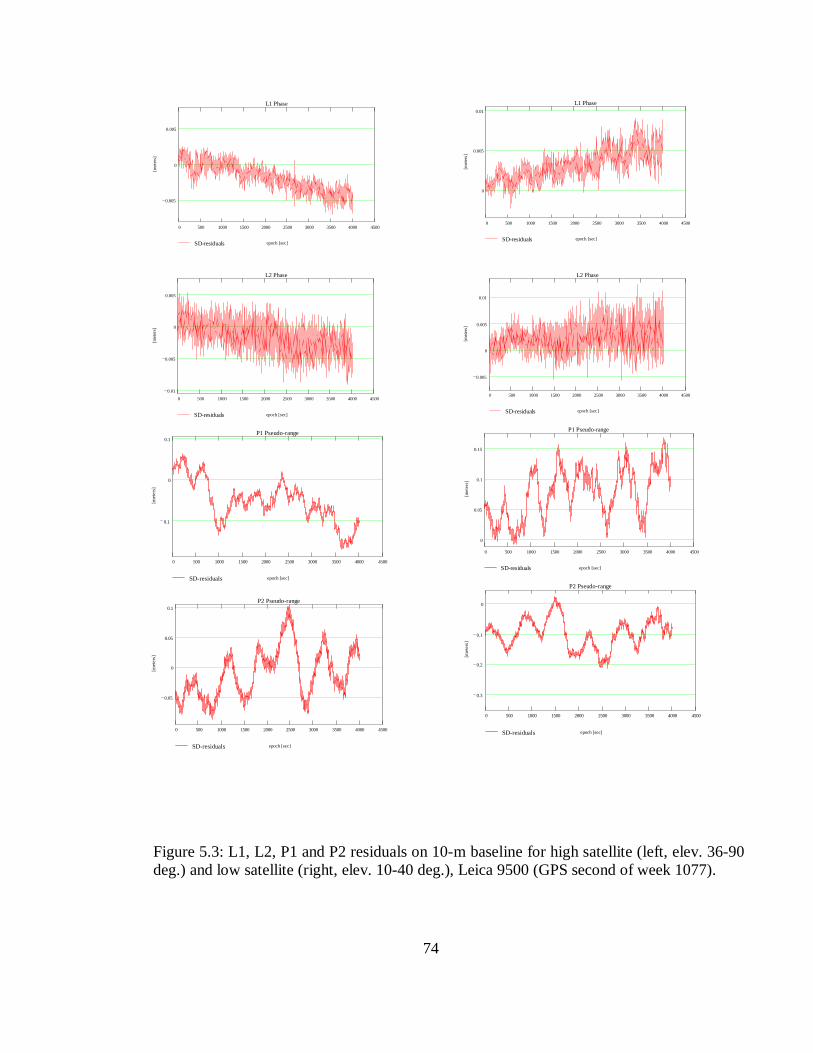
74

0 500 1000 1500 2000 2500 3000 3500 4000 4500

0.005

0

0.005

SD-residuals

L1 Phase

epoch [sec]

[met

ers]

0 500 1000 1500 2000 2500 3000 3500 4000 4500

0

0.005

0.01

SD-residuals

L1 Phase

epoch [sec]

[met

ers]

0 500 1000 1500 2000 2500 3000 3500 4000 4500

0.01

0.005

0

0.005

SD-residuals

L2 Phase

epoch [sec]

[met

ers]

0 500 1000 1500 2000 2500 3000 3500 4000 4500

0.1

0

0.1

SD-residuals

P1 Pseudo-range

epoch [sec]

[me

ters

]

0 500 1000 1500 2000 2500 3000 3500 4000 4500

0.05

0

0.05

0.1

SD-residuals

P2 Pseudo-range

epoch [sec]

[me

ters

]

0 500 1000 1500 2000 2500 3000 3500 4000 4500

0.005

0

0.005

0.01

SD-residuals

L2 Phase

epoch [sec]

[met

ers]

0 500 1000 1500 2000 2500 3000 3500 4000 4500

0

0.05

0.1

0.15

SD-residuals

P1 Pseudo-range

epoch [sec]

[me

ters

]

0 500 1000 1500 2000 2500 3000 3500 4000 4500

0.3

0.2

0.1

0

SD-residuals

P2 Pseudo-range

epoch [sec]

[me

ters

]

Figure 5.3: L1, L2, P1 and P2 residuals on 10-m baseline for high satellite (left, elev. 36-90 deg.) and low satellite (right, elev. 10-40 deg.), Leica 9500 (GPS second of week 1077).

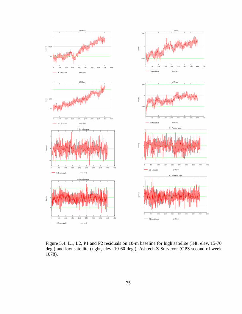
75

0 500 1000 1500 2000 2500 3000 3500 4000 4500

0.01

0.005

0

SD-residuals

L1 Phase

epoch [sec]

[met

ers]

0 500 1000 1500 2000 2500 3000 3500 4000 4500

0.005

0

0.005

SD-residuals

L1 Phase

epoch [sec]

[met

ers]

0 500 1000 1500 2000 2500 3000 3500 4000 4500

0.01

0.005

0

SD-residuals

L2 Phase

epoch [sec]

[met

ers]

0 500 1000 1500 2000 2500 3000 3500 4000 4500

1

0

1

SD-residuals

P1 Pseudo-range

epoch [sec]

[me

ters

]

0 500 1000 1500 2000 2500 3000 3500 4000 4500

1

0

1

SD-residuals

P2 Pseudo-range

epoch [sec]

[me

ters

]

0 500 1000 1500 2000 2500 3000 3500 4000 4500

0.005

0

0.005

SD-residuals

L2 Phase

epoch [sec]

[met

ers]

0 500 1000 1500 2000 2500 3000 3500 4000 4500

1

0

1

SD-residuals

P1 Pseudo-range

epoch [sec]

[me

ters

]

0 500 1000 1500 2000 2500 3000 3500 4000 4500

1

0

1

SD-residuals

P2 Pseudo-range

epoch [sec]

[me

ters

]

Figure 5.4: L1, L2, P1 and P2 residuals on 10-m baseline for high satellite (left, elev. 15-70 deg.) and low satellite (right, elev. 10-60 deg.), Ashtech Z-Surveyor (GPS second of week 1078).

76

0 500 1000 1500 2000 2500

0.002

0

0.002

0.004

SD-residuals

L1 Phase

epoch [sec]

[met

ers]

0 500 1000 1500 2000 2500

0.004

0.002

0

0.002

0.004

SD-residuals

L1 Phase

epoch [sec]

[met

ers]

0 500 1000 1500 2000 2500

0.005

0

0.005

SD-residuals

L2 Phase

epoch [sec]

[met

ers]

0 500 1000 1500 2000 2500

1

0.5

0

0.5

SD-residuals

P1 Pseudo-range

epoch [sec]

[me

ters

]

0 500 1000 1500 2000 2500

1

0.5

0

0.5

1

SD-residuals

P2 Pseudo-range

epoch [sec]

[me

ters

]

0 500 1000 1500 2000 2500

0.005

0

0.005

SD-residuals

L2 Phase

epoch [sec]

[met

ers]

0 500 1000 1500 2000 2500

0.5

0

0.5

1

SD-residuals

P1 Pseudo-range

epoch [sec]

[me

ters

]

0 500 1000 1500 2000 2500

1

0

1

SD-residuals

P2 Pseudo-range

epoch [sec]

[me

ters

]

Figure 5.5: L1, L2, P1 and P2 residuals on 10-m baseline for high satellite (left, elev. 20-90 deg.) and low satellite (right, elev. 10-60 deg.), Trimble 4000SSE (GPS second of week 1078).

77

0 500 1000 1500 2000 2500 3000 3500 4000

0

0.005

SD-residuals

L1 Phase

epoch [sec]

[met

ers]

0 500 1000 1500 2000 2500 3000 3500 4000

0.006

0.004

0.002

0

0.002

SD-residuals

L1 Phase

epoch [sec]

[met

ers]

0 500 1000 1500 2000 2500 3000 3500 4000

0.004

0.002

0

0.002

0.004

SD-residuals

L2 Phase

epoch [sec]

[met

ers]

0 500 1000 1500 2000 2500 3000 3500 4000

0.5

0

0.5

SD-residuals

P1 Pseudo-range

epoch [sec]

[me

ters

]

0 500 1000 1500 2000 2500 3000 3500 4000

0.5

0

0.5

1

SD-residuals

P2 Pseudo-range

epoch [sec]

[me

ters

]

0 500 1000 1500 2000 2500 3000 3500 4000

0.005

0

0.005

SD-residuals

L2 Phase

epoch [sec]

[met

ers]

0 500 1000 1500 2000 2500 3000 3500 4000

0.5

0

0.5

SD-residuals

P1 Pseudo-range

epoch [sec]

[me

ters

]

0 500 1000 1500 2000 2500 3000 3500 4000

1

0

1

SD-residuals

P2 Pseudo-range

epoch [sec]

[me

ters

]

Figure 5.6: L1, L2, P1 and P2 residuals on 10-m baseline for high satellite (left, elev. 15-70 deg.) and low satellite (right, elev. 10-35 deg.), Trimble 4000SSI (GPS second of week 1078).

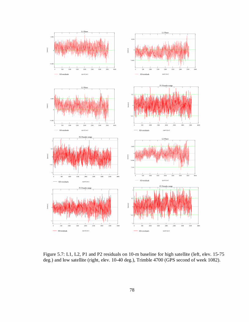
78

0 500 1000 1500 2000 2500 3000 3500 4000

0.005

0

0.005

SD-residuals

L1 Phase

epoch [sec]

[met

ers]

0 500 1000 1500 2000 2500 3000 3500 4000

0.005

0

0.005

SD-residuals

L1 Phase

epoch [sec]

[met

ers]

0 500 1000 1500 2000 2500 3000 3500 4000

0.005

0

0.005

SD-residuals

L2 Phase

epoch [sec]

[met

ers]

0 500 1000 1500 2000 2500 3000 3500 4000

0.5

0

0.5

SD-residuals

P1 Pseudo-range

epoch [sec]

[me

ters

]

0 500 1000 1500 2000 2500 3000 3500 4000

1

0.5

0

0.5

1

SD-residuals

P2 Pseudo-range

epoch [sec]

[me

ters

]

0 500 1000 1500 2000 2500 3000 3500 4000

0.01

0.005

0

0.005

SD-residuals

L2 Phase

epoch [sec]

[met

ers]

0 500 1000 1500 2000 2500 3000 3500 4000

1

0

1

SD-residuals

P1 Pseudo-range

epoch [sec]

[me

ters

]

0 500 1000 1500 2000 2500 3000 3500 4000

1

0.5

0

0.5

1

SD-residuals

P2 Pseudo-range

epoch [sec]

[me

ters

]

Figure 5.7: L1, L2, P1 and P2 residuals on 10-m baseline for high satellite (left, elev. 15-75 deg.) and low satellite (right, elev. 10-40 deg.), Trimble 4700 (GPS second of week 1082).

79

CHAPTER 6

THE ALTERNATIVE VARIANCE-COVARIANCE MATRIX

6.1 Precise Positioning Estimators Based on the Alternative Variance-Covariance (V-C) Matrix.

Starting from Equation (4.2), which represents the final formulation of single-differences we have:

• For carrier phase observations:

, , , ,

1( ) ( ) ( )k k k k

i j i j i j i jt t f t Nρ δλ

Φ = + + (6.1)

where

, ( ) ( ) ( )k k ki j j it t tΦ = Φ − Φ

, ( ) ( ) ( )k k ki j j it t tρ ρ ρ= −

, ( ) ( ) ( )i j R Rj it t tδ δ δ= −

,k k ki j j iN N N= −

• For pseudo-range observations:

, , ,( ) ( ) ( )k k ki j i j i jR t t f tρ δ= + (6.2)

where

, ( ) ( ) ( )k k ki j j iR t R t R t= −

, ( ) ( ) ( )k k ki j j it t tρ ρ ρ= −

From (6.1), and considering that , ,k k

i j i jf Nδ + (lumped receiver clock and SD-

ambiguity) is assumed to be known here from the previous adjustment (refer Section 4.2), we set up our functional model based on carrier phase observations as follows:

, , , ,

1( ) ( ( ) ) ( )k k k k

i j i j i j i jt f t N t eδ ρλ

Φ − + = + (6.3)

In analogy to carrier phase observations, we set up our functional model based on pseudo-range observations as follows:

, , ,( ) ( ) ( )k k ki j i j i jR t f t t eδ ρ− = + (6.4)

where 1/2 1/22 2 2 2 2 2

, ( ) ( ) ( ) ( ) ( ) ( ) ( )k k k k k k ki j j j j i i it X X Y Y Z Z X X Y Y Z Zρ = − + − + − − − + − + −

0

( )T

aA

Ξ−Ξ

∂ Ξ=∂Ξ

0ξ = Ξ − Ξ

, ( )ki jf tδ - given in meters here

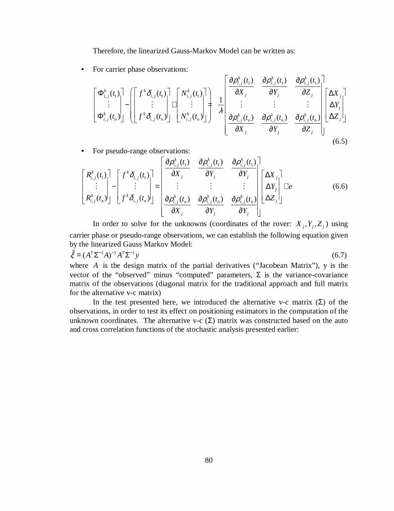
80

Therefore, the linearized Gauss-Markov Model can be written as:

• For carrier phase observations:

, 1 , 1 , 1

, 1 , 1 , 1

, , , , , ,

( ) ( ) ( )

( ) ( ) ( )1

( ) ( ) ( ) ( ) ( ) ( )

k k ki j i j i j

k k kj j ji j i j i j

k k k k k ki j n i j n i j n i j n i j n i j n

j j j

t t t

X Y Zt f t N t

t f t N t t t t

X Y Z

ρ ρ ρδ

λδ ρ ρ ρ

∂ ∂ ∂

∂ ∂ ∂ Φ − + = Φ ∂ ∂ ∂ ∂ ∂ ∂

⋮ ⋮ ⋮ ⋮ ⋮ ⋮

j

j

j

X

Y

Z

∆ ∆ ∆

(6.5) • For pseudo-range observations:

, 1 , 1 , 1

, 1 , 1

, , , , ,

( ) ( ) ( )

( ) ( )

( ) ( ) ( ) ( ) ( )

k k ki j i j i j

k kj j ji j i j j

j

k k k k ki j n i j n ji j n i j n i j n

j j j

t t t

X Y YR t f t X

Y e

R t f t Zt t t

X Y Y

ρ ρ ρδ

δ ρ ρ ρ

∂ ∂ ∂ ∂ ∂ ∂ ∆

− = ∆ + ∆ ∂ ∂ ∂

∂ ∂ ∂

⋮ ⋮ ⋮ ⋮ ⋮ (6.6)

In order to solve for the unknowns (coordinates of the rover: , ,j j jX Y Z ) using

carrier phase or pseudo-range observations, we can establish the following equation given by the linearized Gauss Markov Model:

1 1 1ˆ ( )T TA A A yξ − − −= Σ Σ (6.7) where A is the design matrix of the partial derivatives (“Jacobean Matrix”), y is the vector of the “observed” minus “computed” parameters, Σ is the variance-covariance matrix of the observations (diagonal matrix for the traditional approach and full matrix for the alternative v-c matrix)

In the test presented here, we introduced the alternative v-c matrix (Σ) of the observations, in order to test its effect on positioning estimators in the computation of the unknown coordinates. The alternative v-c (Σ) matrix was constructed based on the auto and cross correlation functions of the stochastic analysis presented earlier:

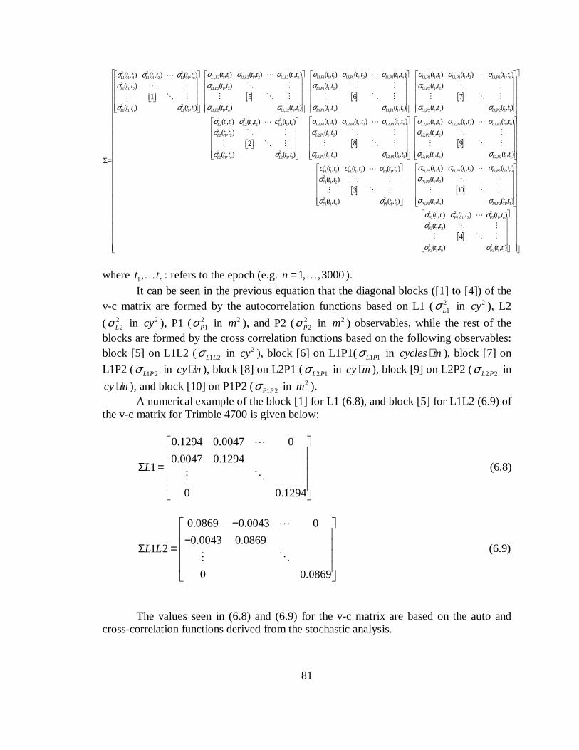
81

[ ]

2 2 21, 2 1 1 1, 2 1 2 1, 2 1 1, 11 1 1 1 1 2 1 1

21, 2 1 21 1 2

2 21, 2 1 1, 2 1 11 1 1 1 1

( , ) ( , ) ( , ) (( , ) ( , ) ( , )

( , )( , )

5

( , ) ( , )( , ) ( , )

1

L L L L L L n L PL L L n

L LL

L L n L LL n L

t t t t t t tt t t t t t

t tt t

t t t tt t t t

σ σ σ σσ σ σσσ

σ σσ σ

Σ=

⋯⋯

⋱ ⋮⋱ ⋮

⋮ ⋱ ⋮⋮ ⋱ ⋮ [ ] [ ]

1 1 1, 1 1 2 1, 1 1 1, 2 1 1 1, 2 1 2 1, 2 1

1, 1 1 2 1, 2 1 2

1, 1 1 1, 1 1 1 1, 2 1 1, 2 1 1

22 1 1

, ) ( , ) ( , ) ( , ) ( , ) ( , )

( , ) ( , )

6 7

( , ) ( , ) ( , ) ( , )

( ,

L P L P n L P L P L P n

L P L P

L P n L P L P n L P

L

t t t t t t t t t t t

t t t t

t t t t t t t t

t t

σ σ σ σ σσ σ

σ σ σ σ

σ

⋯ ⋯

⋱ ⋮ ⋱ ⋮

⋮ ⋱ ⋮ ⋮ ⋱ ⋮

[ ]

2 22, 1 1 1 2, 1 1 2 2, 1 1 2, 2 1 1 2, 22 1 2 2 1

22, 1 1 22 1 2

2 22, 1 1 2, 1 1 12 1 2 1 1

( , ) ( , ) ( , ) ( , ) () ( , ) ( , )

( , )( , )

8

( , ) ( , )( , ) ( , )

2

L P L P L P n L P L PL L n

L PL

L P n L PL n L

t t t t t t t tt t t t

t tt t

t t t tt t t t

σ σ σ σ σσ σσσ

σ σσ σ

⋯⋯

⋱ ⋮⋱ ⋮

⋮ ⋱ ⋮⋮ ⋱ ⋮ [ ]

[ ]

1 2 2, 2 1

2, 2 1 2

2, 2 1 2, 2 1 1

2 2 21, 2 1 1 1, 2 1 2 1, 21 1 1 1 1 2 1 1

21 1 2

2 21 1 1 1 1

, ) ( , )

( , )

9

( , ) ( , )

( , ) ( , ) (( , ) ( , ) ( , )

( , )

3

( , ) ( , )

L P n

L P

L P n L P

P P P P P PP P P n

P

P n P

t t t t

t t

t t t t

t t t tt t t t t t

t t

t t t t

σσ

σ σ

σ σ σσ σ σσ

σ σ

⋯

⋱ ⋮

⋮ ⋱ ⋮

⋯⋯

⋱ ⋮

⋮ ⋱ ⋮ [ ]

[ ]

1

1, 2 1 2

1, 2 1 1, 2 1 1

2 2 22 1 1 2 1 2 2 1

22 1 2

2 22 1 2 1 1

, )

( , )

10

( , ) ( , )

( , ) ( , ) ( , )

( , )

4

( , ) ( , )

n

P P

P P n P P

P P P n

P

P n P

t t

t t

t t t t

t t t t t t

t t

t t t t

σ

σ σ

σ σ σσ

σ σ

⋱ ⋮

⋮ ⋱ ⋮

⋯

⋱ ⋮

⋮ ⋱ ⋮

where 1, nt t… : refers to the epoch (e.g. 1, ,3000n = … ).

It can be seen in the previous equation that the diagonal blocks ([1] to [4]) of the v-c matrix are formed by the autocorrelation functions based on L1 (2

1Lσ in 2cy ), L2

( 22Lσ in 2cy ), P1 ( 2

1Pσ in 2m ), and P2 ( 22Pσ in 2m ) observables, while the rest of the

blocks are formed by the cross correlation functions based on the following observables: block [5] on L1L2 ( 1 2L Lσ in 2cy ), block [6] on L1P1( 1 1L Pσ in cycles m⋅ ), block [7] on

L1P2 ( 1 2L Pσ in cy m⋅ ), block [8] on L2P1 ( 2 1L Pσ in cy m⋅ ), block [9] on L2P2 ( 2 2L Pσ in

cy m⋅ ), and block [10] on P1P2 ( 1 2P Pσ in 2m ). A numerical example of the block [1] for L1 (6.8), and block [5] for L1L2 (6.9) of

the v-c matrix for Trimble 4700 is given below:

0.1294 0.0047 0

0.0047 0.12941

0 0.1294

L

Σ =

⋯

⋮ ⋱ (6.8)

0.0869 0.0043 0

0.0043 0.08691 2

0 0.0869

L L

− − Σ =

⋯

⋮ ⋱ (6.9)

The values seen in (6.8) and (6.9) for the v-c matrix are based on the auto and

cross-correlation functions derived from the stochastic analysis.

82

After we have introduced the v-c matrix of the observations into (6.7) and solved for the unknowns ( , ,j j jX Y Z ), we compute the residual vector given by the following

equation: ˆe y Aξ= −ɶ (6.10)

Then, we compute the variance component estimate given by: 1

20ˆ

Te e

n mσ

−Σ=−ɶ ɶ

(6.11)

where n is the number of observations, m is the number of parameter to determine (3). The dispersion matrix was computed by:

2 1 10

ˆ ˆ ( )TD A Aξ σ − −= Σ (6.12)

Finally we computed the standard deviation a posteriori given by: ˆˆ .apost Dσ ξ= (6.13)

6.2 Analysis and Results

As mentioned earlier, based on the stochastic analysis we proposed an alternative v-c matrix, in order to test its effect in precise positioning estimators. Then, we compare the SD positioning results from the alternative v-c matrix with those from the traditional approach. It is important to point out here that, according to the model proposed by Euler and Goad, 1991, (traditional approach), where the standard deviation is an exponential function of the elevation angle, the variance covariance matrix of the observations (i.e. one way) remains diagonal but the variances may vary from satellite to satellite (elevation angle dependency). In other words, if the model is applied to observations coming from low satellites less weight must be applied in comparison with observations coming from high satellites (with larger weights). However we decided to compute coordinates of the different stations (different types of GPS receivers) only for high satellites, assuming the corresponding values of the variances for the carrier phases

2 3 21 (5.258 10 )L cyσ −= ⋅ , 2 3 2

2 (8.19 10 )L cyσ −= ⋅ and ( 2 2 21 2 (0.5 )P P mσ σ= = ) for the pseudo-

ranges. Those coordinates were computed considering one of the GPS receivers as “the

base” and the other one as “the rover”; an example for zero and short baseline measurements is provided. The coordinates of the stations were previously determined in order to carry out the stochastic analysis; therefore, at first instance they were used as approximated values in order to compute for the new “rover” coordinates. It is important to point out here that the small “biases” observed in the SD-residuals from some receivers (discussed in the stochastic analysis) were removed; therefore, the alternative v-c matrix does not contain those biases.

As a first step, we determine the coordinates of the receivers and their corresponding variance component (standard deviation a posteriori) using the traditional approach (diagonal variance-covariance matrix) assuming no correlation among them. In other words, we provide the solution for each one of the observables separately. Results

83

using the traditional approach for L1 and P1 observables can be seen in Table 6.1 for zero baseline measurements, and in Table 6.5 for short (10 m) baseline measurements. It is important to mention here that for short baseline measurements (10 m), we provided results only for T/JPS Legacy as a representative sample. As a second step, we compute the coordinates of the stations and their corresponding variance component, using the alternative v-c matrix. Here, we also provided a solution based on L1 and P1 observables (separately). Results using the alternative v-c matrix are shown in Table 6.2 for zero baseline measurements, and in Table 6.6 for short (10 m) baseline measurements. In both cases (step one and two), we considered a 50 minutes (3000 epochs) window of SD-observations as a representative sample. The dimension of the resulting variance-covariance matrices (traditional approach and alternative) was 3000x3000. It can be observed in Table 6.1 (traditional approach) and 6.2 (alternative v-c matrix) that the estimate of the positioning accuracy (given by the standard deviation a posteriori) increases according to the type of the observable, resulting in values of the centimeter level for L1, and in values of several centimeters for P1. In general, in terms of coordinates they are similar between receivers and same type of observables for both cases (traditional approach and alternative v-c matrix). This fact can also observe in Tables 5.1 and 5.2 where the values of the distances were computed with the difference between coordinates of the receivers. Table 6.1 indicates that Trimble 4000SSE shows the shortest distance (0.0005 m), which is very close to the value of “true distance” (0.0 m); the rest of the receivers show distances in the order of 2-9 mm (for L1 phase). On the other hand, using P1 code all the receivers show a distance between 3-4 cm, except for Ashtech Z-S, which shows the bigger distance 7 cm. Table 6.2 indicates that all the receivers show distance within 9-22 mm for L1, and within 4-5 cm for P1, except for Ashtech (11 cm.). In general, the results obtained using the traditional approach (see Table 6.1) in terms of distance are better with respect to the “true value” in comparison with the obtained using the alternative v-c matrix (see Table 6.2), but they might perhaps be more optimistic.

Table 6.1: Coordinates using a 50 min observation window (traditional approach).

Coordinates Standard Deviation. (m) GPS Receiver

Obs. Type

X Y Z X Y Z

Distance (m)

L1 592929.5459 -4856724.6309 4078214.8157 0.0013 0.0019 0.0010 0.0005 T4000 SSE

P1 592929.5736 -4856724.6513 4078214.7981 0.0711 0.0800 0.0673 0.0382 L1 592929.5447 -4856724.6329 4078214.8141 0.0011 0.0017 0.0008 0.0024 T4000

SSI P1 592929.5609 -4856724.6697 4078214.8103 0.1031 0.1117 0.0957 0.0414 L1 592929.5485 -4856724.6357 4078214.8159 0.0018 0.0028 0.0009 0.0050 Leica

9500 P1 592929.5697 -4856724.6414 4078214.8002 0.1001 0.1135 0.0996 0.0299 L1 592929.5498 -4856724.6320 4078214.8116 0.0025 0.0036 0.0021 0.0054 T/Javad

Legacy P1 592929.5632 -4856724.6524 4078214.8451 0.1045 0.1126 0.1000 0.0402 L1 592929.5431 -4856724.6318 4078214.8102 0.0017 0.0026 0.0010 0.0060

T4700 P1 592929.5689 -4856724.6516 4078214.8319 0.1116 0.1201 0.1067 0.0346 L1 592939.1977 -4856716.7434 4078221.4689 0.0015 0.0016 0.0014 0.0009 Ashtech

ZS P1 592939.1522 -4856716.7807 4078221.5061 0.0925 0.0997 0.0823 0.0709

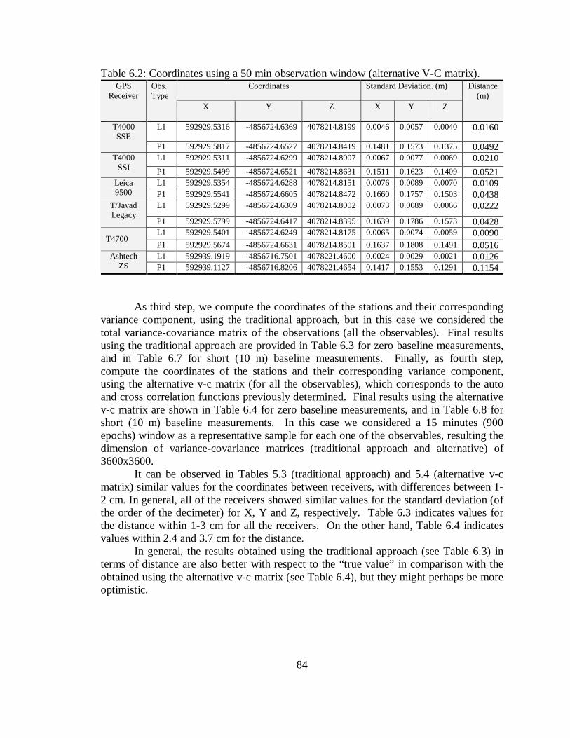
84

Table 6.2: Coordinates using a 50 min observation window (alternative V-C matrix). Coordinates Standard Deviation. (m) GPS

Receiver Obs. Type

X Y Z X Y Z

Distance (m)

L1 592929.5316 -4856724.6369 4078214.8199 0.0046 0.0057 0.0040 0.0160 T4000 SSE

P1 592929.5817 -4856724.6527 4078214.8419 0.1481 0.1573 0.1375 0.0492 L1 592929.5311 -4856724.6299 4078214.8007 0.0067 0.0077 0.0069 0.0210 T4000

SSI P1 592929.5499 -4856724.6521 4078214.8631 0.1511 0.1623 0.1409 0.0521 L1 592929.5354 -4856724.6288 4078214.8151 0.0076 0.0089 0.0070 0.0109 Leica

9500 P1 592929.5541 -4856724.6605 4078214.8472 0.1660 0.1757 0.1503 0.0438 L1 592929.5299 -4856724.6309 4078214.8002 0.0073 0.0089 0.0066 0.0222 T/Javad

Legacy P1 592929.5799 -4856724.6417 4078214.8395 0.1639 0.1786 0.1573 0.0428 L1 592929.5401 -4856724.6249 4078214.8175 0.0065 0.0074 0.0059 0.0090

T4700 P1 592929.5674 -4856724.6631 4078214.8501 0.1637 0.1808 0.1491 0.0516 L1 592939.1919 -4856716.7501 4078221.4600 0.0024 0.0029 0.0021 0.0126 Ashtech

ZS P1 592939.1127 -4856716.8206 4078221.4654 0.1417 0.1553 0.1291 0.1154

As third step, we compute the coordinates of the stations and their corresponding

variance component, using the traditional approach, but in this case we considered the total variance-covariance matrix of the observations (all the observables). Final results using the traditional approach are provided in Table 6.3 for zero baseline measurements, and in Table 6.7 for short (10 m) baseline measurements. Finally, as fourth step, compute the coordinates of the stations and their corresponding variance component, using the alternative v-c matrix (for all the observables), which corresponds to the auto and cross correlation functions previously determined. Final results using the alternative v-c matrix are shown in Table 6.4 for zero baseline measurements, and in Table 6.8 for short (10 m) baseline measurements. In this case we considered a 15 minutes (900 epochs) window as a representative sample for each one of the observables, resulting the dimension of variance-covariance matrices (traditional approach and alternative) of 3600x3600.

It can be observed in Tables 5.3 (traditional approach) and 5.4 (alternative v-c matrix) similar values for the coordinates between receivers, with differences between 1-2 cm. In general, all of the receivers showed similar values for the standard deviation (of the order of the decimeter) for X, Y and Z, respectively. Table 6.3 indicates values for the distance within 1-3 cm for all the receivers. On the other hand, Table 6.4 indicates values within 2.4 and 3.7 cm for the distance.

In general, the results obtained using the traditional approach (see Table 6.3) in terms of distance are also better with respect to the “true value” in comparison with the obtained using the alternative v-c matrix (see Table 6.4), but they might perhaps be more optimistic.

85

Table 6.3: Coordinates using a 15 min observation window (traditional approach). Coordinates Standard Deviation. (m) GPS

Receiver Obs.

L1, L2, P1&P2

X Y Z X Y Z

Dist. (m)

4000SSE √ 592929.5342 -4856724.6211 4078214.8229 0.0412 0.0499 0.0371 0.0173

4000SSI √ 592929.5401 -4856724.6417 4078214.8166 0.0528 0.0613 0.0478 0.0160

Lei 9500 √ 592929.5298 -4856724.6156 4078214.8305 0.0514 0.0598 0.0473 0.0271

T/Javad √ 592929.5319 -4856724.6431 4078214.8317 0.0492 0.0612 0.4105 0.0244

T4700 √ 592929.5561 -4856724.6501 4078214.8357 0.0685 0.0716 0.0573 0.0293

Ashtech √ 592939.2157 -4856716.7563 4078221.4871 0.0576 0.0683 0.0507 0.0295

Table 6.4: Coordinates using a 15 min observation window (alternative V-C matrix)

Coordinates Standard Deviation. (m) GPS Receiver

Obs. L1, L2, P1&P2

X Y Z X Y Z

Dist. (m)

4000SSE √ 592929.5609 -4856724.6426 4078214.8001 0.0847 0.0934 0.0706 0.0242

4000SSI √ 592929.5601 -4856724.6468 4078214.7967 0.1035 0.1147 0.0960 0.0288

Lei 9500 √ 592929.5677 -4856724.6475 4078214.8406 0.1108 0.1213 0.1042 0.0368

T/Javad √ 592929.5614 -4856724.6430 4078214.8324 0.0975 0.1168 0.0896 0.0256

T4700 √ 592929.5665 -4856724.6502 4078214.7996 0.1117 0.1032 0.1080 0.0314

Ashtech √ 592939.1769 -4856716.7583 4078221.4450 0.0981 0.1124 0.0900 0.0351

As mentioned earlier, a representative sample is presented for short baseline measurements. It can be observed in Table 6.5 (traditional approach) and 5.6 (alternative v-c matrix) that the estimate of the positioning accuracy increases according to the type of the observable, which results in values of the centimeter level for L1, and in values of several centimeters for P1. In general, using the two approaches, the values of the coordinates they are similar between receivers and same type of observables. Again we can also observe in Tables 5.5 and 5.6 the values of the distances computed with the difference between coordinates of the receivers. Table 6.5 and 5.6 indicate that for the two approaches the value of the computed distance is very close to the value of “true distance” (9.9950 m) for L1 and P1, respectively.

Tables 5.7 and 5.8 indicates that using the two approaches, similar values in terms of coordinates and distances were found; and they differ only in terms of standard deviation.

86

The results obtained using the traditional approach (see Tables 5.5 and 5.7) in terms of distance are a little better with respect to the “true value” in comparison with the obtained using the alternative v-c matrix (see Table 6.6 and Table 6.8).

In general, for zero and short baseline examples the traditional approach showed better results in comparison with the alternative v-c matrix; however, this is a typical case study and more research is needed in order to revise this approach. Table 6.5: Coordinates using a 50 min observation window (traditional approach).

Coordinates Standard Deviation. (m) GPS

Receiver

Obs. L1 & P1

X Y Z X Y Z

Distance (m)

L1 592939.4917 -4856723.7999 4078214.2818 0.0216 0.0158 0.0120 9.9985

T/Javad P1 592939.4373 -4856723.3317 4078213.88056 0.1286 0.1129 0.1106 10.0306

Table 6.6: Coordinates using a 50 min observation window (alternative V-C matrix).

Coordinates Standard Deviation. (m) GPS

Receiver

Obs. L1 & P1

X Y Z X Y Z

Distance (m)

L1 592939.5001 -4856723.8110 4078214.2817 0.0335 0.0302 0.0298 10.0059

T/Javad P1 592939.4437 -4856723.3410 4078213.8827 0.1503 0.1417 0.1365 10.0354

Table 6.7: Coordinates using a 15 min observation window (traditional approach).

Coordinates Standard Deviation. (m) GPS Receiver

Obs. L1

X Y Z X Y Z

Distance (m)

T/Javad √ 592939.4327 -4856723.3527 4078213.8900 0.0571 0.0593 0.0496 10.0221

Table 6.8: Coordinates using a 15 min observation window (alternative V-C matrix).

Coordinates Standard Deviation. (m) GPS Receiver

Obs. L1

X Y Z X Y Z

Distance (m)

T/Javad √ 592939.4455 -4856723.3967 4078213.8523 0.1134 0.1086 0.0975 10.0327

87

6.3 Summary and Conclusions

Six pairs GPS receivers, classified as geodetic grade, were tested, in order to accomplish the analysis of the stochastic properties of different types of GPS observable. Based on the results presented for the GPS static surveys (zero baseline) it can be concluded that:

• In general, most of the SD-residuals obtained from zero baseline measurements are smaller for high satellites in comparison with low (in the order of the millimeter) for the L1 and L2 carrier phases, this fact can be attributed to the elevation angle dependence which is expected according to (Euler and Goad 1991; Tiberius et al., 1999).

• The SD-residuals derived from zero baseline measurements are smaller in comparison with those showed for the 10-m baseline example.

• The presence of small biases (of the mm level) was shown in some of the SD- residuals (zero baseline) for L1 and L2 carrier phases and for P1 and P2 (of the cm level), which might be attributed to some remaining systematic effects.

• In terms of time correlation it can be concluded that all the receivers showed short correlation times (<5 seconds); for high and low satellite on L1, L2, P1 and P2 except for Ashtech Z-S which showed large correlation time (> 5 seconds) only on P1 for high and low satellite, respectively.

• The only observable that showed no virtual correlation time was L1 (1 sec) Large correlation times indicate significant internal data filtering inside the receiver.

• The noise level for all the receivers is in the order of the millimeter for carrier phases, and of the order of the decimeter for pseudo-ranges, which is comparable to those obtained by Bona, 2000.

• From the cross correlation results we can observe that if the correlation is present between L1 and L2 pseudo-ranges or carrier phases, it is positive, which is comparable to the results obtained by (Bona, 2000). Receivers such as, Trimble 4000SSI, Topcon/JPS Legacy, Trimble 4700 and Ashtech Z-Surveyor showed the big correlation between carriers phases in comparison with the rest of the receivers; here, the ranges of correlation coefficients for L1 and L2 varies from 0.16 to 0.37.

• In terms of positioning estimators, it can be concluded that for zero and short baselines examples the results obtained using the traditional approach are more optimistic in comparison with those obtained using the alternative v-c matrix that accounts for empirical correlation among the observable. This fact might indicate the importance of considering the correlation aspects (auto and cross correlation) provided by the stochastic analysis of the GPS observable. However, this is a typical case study and more research is needed in order to revise this approach. 6.4 Suggestions and Recommendation for Further Research

• Some biases and drifts experienced for Leica 9500 (on L1 and L2) and Ashtech Z-S (on P1 and P2) that may require further investigation.

• The presence of time correlation for the different types of observables can be an important fact for kinematic applications (e.g. ambiguity resolution problem).

88

• In practical applications, the data-sampling interval is another factor to consider when correlation time is 5 or more seconds, while using 1 second sampling.

• Even though, we introduced an alternative v-c matrix as part of the stochastic model for precise GPS positioning (full matrix) for GPS positioning applications, this is a typical case study and more research is needed in order to revise this approach.

• Analysis of the solution repeatability with traditional approach vs. alternative v-c Matrix is another aspect that may be investigated.

• When L5 frequency (second civilian signal) becomes available (2005), it will be possible in principle to recover uncorrelated L1 &L2 and C1 & C2.

89

BIBLIOGRAPHY

Ashby N (1987): Relativistic effects in the Global Positioning System. In: Relativistic effects in geodesy, Proceedings of the IAG Symposia of the XIX General Assambly of the IUGG, Vancouver, Canada, August 10-22, Vol. 1:41-50. Bletzacker, FR. (1985): Reduction of Multipath Contamination in a Geodetic GPS Receiver, Proceedings of the 1st International Symposium on Precise Positioning with the GPS, Rockville, Maryland. Bona P., Precision, cross correlation and time correlation of GPS phase and code observations, GPS solutions, 2000, Vol. 4, No. 2. Bona P.and C. Tiberius (2000a)., An experimental assessment of observation cross correlation in dual frequency GPS receivers, Proceedings of ION GPS, Salt Lake City, Utah, September 19-21. Bona P. and C. Tiberius (2000b)., An experimental comparison of noise characteristics of seven high-end dual frequency GPS receiver sets, Proceedings of IEEE PLANS2000, San Diego, California, March 13-16, 2000, pp.237-244. Bowen, R. (1986): GPS Control System Accuracies, GPS papers, Vol. III, Institute of Navigation, Washington, D.C., pp. 241-247. Brunner, F. K., and Welsch W. M., (1993): Effect of Troposphere on GPS Measurements, GPS World, January, 1993. Brown, R. G. and P. Y. C. Hwang (1992): Introduction to Random Signals and Applied Kalman Filtering. John Wiley and Sons, Inc., New York. Euler H. and Goad C. C. (1991) On optimal filtering of GPS dual-frequency observations without using orbit information. Bull. Geod. Berlin, Germany, Vol. 65, pp. 130-143. Gelb A. (ed.), Applied Optimal Estimation, Cambridge, MA: MIT Press, 1974 Goad C., L. Goodmann (1974): A Modified Hopfield tropospheric Refraction Correction Model, paper presented at the AGU, Annual Fall meeting, San Francisco, California, December 12-17. Gourevitch S. (1996) Measuring GPS Receiver Performance: A New Approach. GPS World, Vol. 7, No. 10, pp.56-52. GPS World, January 2001, Vol. 12 No. 1 pp. 32-47.

90

Grejner-Brzezinska D., 2001, GPS Instrumentation Issues, Chapter 10 in Manual of Geographical Science and Technology, Bossler (Ed.), taylor Francois Books, in press. Grejner-Brzezinska D., and Toth C. (2000): Interference and Multipath Effects on GPS/INS Positioning Results, Proc. ION GPS, September 19-21, Salt Lake City, Utah, CD ROM. Gurtner W., RINEX: The Receiver Independent Exchange Format, GPS World, July 1994, pp. 48-52. Hofmann-Wellenhof, B, H. Lichtenegger, and J. Collins (2001): Global Positioning System, Theory and Practice. Springer-Verlag, Wien. http://igscb.jpl.nasa.gov http://leica-geosystems.com http://nationaldefense.ndia.org http://topconps.com http://www.ashtech.com http://www.gfz-postdam.com http://www.trimble.com Jekeli C. (2000a): Inertial Navigation System. Walter deGruyter & Co., Berlin. Jekeli C. (2000b): Lecture notes in Spectral Methods in Gravimetric Geodesy. Johnson, R. C. (editor), Antenna Engineering Handbook, 3rd edition, 1993, McGraw Hill, New York, NY. Langley R. B., The GPS Receiver System Noise, GPS world, June 1997, pp.40-45. Leick, A., (1990): GPS Satellite Surveying, A Wiley-Interscience publication, John Willey & Sons, New York, NY. Lichtenegger H. (1998): DGPS fundamentals. Reports on geodesy, Warsaw University of technology, 11 (41): 7-19. Moritz, H., Mueller I. (1987): Earth Rotation, Theory and Observation, Ungar, New York, NY. Moritz, H., (1980): Advanced Physical Geodesy. H. Wichmann Verlag, Heidelberg

91

Parkinson B. W. and Spilker J. J. (ed.), Global Positioning System: Theory and Applications, American Institute of Aeronautics and Astronautics, Inc., 1996. Schuper BR., TA Clark (1991): How Different Antennas Affect the GPS Observable, GPS World, 2(10), pp. 32-36. Seeber, G. (1993): Satellite Geodesy. Walter deGruyter & Co., Berlin. Strang, G., Borre, K., (1997): Linear Algebra, Geodesy and GPS, Wellesley-Cambridge Press. Strange W., The Relation of NAD83 Coordinates of the NGS CORS Network to other Types of Coordinates Silverman, B. (1986). Density estimation for statistics and data analysis. Monographs on statistics and applied probability. Chapman and Hall, London. Tiberius, C., Jonkman, N. and Kenselaar, F., The Stochastics of GPS observables, GPS world, Vol. 10, February 1999, pp. 49-54. Wang, J., Stochastic assessment of the GPS measurements for precise positioning, Proceedings of ION GPS, Nashville 1998, pp. 81-89.