analysis of stellar occultation data. ii ... - occult.mit.edu

ANALYSIS OF STELLAR OCCULTATION DATA. II. INVERSION, WITH APPLICATIONTO PLUTO AND TRITON1

J. L. Elliot,2,3

M. J. Person,2and S. Qu

2,4

Received 2002 December 17; accepted 2003March 26

ABSTRACT

We present a method for obtaining atmospheric temperature, pressure, and number density profiles forsmall bodies through inversion of light curves recorded during stellar occultations. This method avoids theassumption that the atmospheric scale height is small compared with the radius of the body, and it includesthe variation of gravitational acceleration with radius. First we derive the integral equations for temperature,scale height, pressure, number density, refractivity, and radius in terms of the light-curve flux. These are thencast into summation form suitable for numerical evaluation. Equations for the errors in these quantitiescaused by Gaussian noise in the occultation light curve are also derived. The method allows for an arbitraryatmospheric boundary condition above the inversion region, and one particular boundary condition isimplemented through least-squares fitting. When the inversion equations are applied to noiseless test data fora simulated isothermal atmosphere, numerical errors in the calculated temperature profile are less than 5parts in 104. Nonisothermal test cases are also presented. We explore the effects of (1) the boundary condi-tion, (2) data averaging (in the time, observer-plane, and body-plane domains), (3) systematic errors in thezero stellar flux level, and (4) light-curve noise on the accuracy of the inversion results. A criterion is presentedfor deciding whether inversion would be an appropriate analysis for a given stellar occultation light curve,and limitations to the radial resolution of the inversion results are discussed. The inversion method is thenemployed on the light curves for the 1988 June 9 occultation by Pluto observed with the Kuiper AirborneObservatory and the 1997 November 4 occultation by Triton observed with the Hubble Space Telescope.Under the (possibly incorrect) assumption that no extinction effects are present in the occultation light curve,the Pluto inversion yields a 110 K isothermal profile down to approximately 1215 km radius, at which point astrong thermal gradient, 3.9 � 0.6 K km�1, abruptly appears, reaching 93 K at the end of the inversion. TheTriton inversion yields a differently shaped profile, which has an upper level thermal gradient, �0.4 K km�1,followed by a �51 K isothermal profile at lower altitudes. The Triton inversion shows wavelike temperaturevariations in the lower atmosphere, with amplitudes of �1 K and wavelengths of �20 km, that could becaused by horizontal or vertical atmospheric waves.

Key words: occultations — planets and satellites: individual (Pluto, Triton)

1. INTRODUCTION

Pluto and Triton both have a tenuous, predominantly N2

atmosphere that is in vapor pressure equilibrium withsurface ice. The extreme sensitivity of the nitrogen vaporpressure to the temperature of the surface ice (Brown &Ziegler 1980) means that large seasonal changes in surfacepressure can accompany changes in insolation and surfacealbedo. Indeed, following the Voyager encounter of theNeptune system in 1989, such changes were predicted forTriton by several authors (Spencer & Moore 1992; Hansen& Paige 1992) and subsequently observed (Elliot et al. 1998,2000a). Vapor pressure equilibrium also has implicationsfor Triton’s atmospheric dynamics (Ingersoll 1990). Simi-larly, Pluto’s large orbital eccentricity (0.25) would lead oneto believe that its atmosphere might undergo collapse as it

recedes from the Sun (perihelion was in 1989); however, thisview has been called into question by Stansberry & Yelle(1999), who modeled the seasonal transition between the �and � phases of N2 ice on Pluto’s surface and found (undercertain assumptions) that its surface pressure may experi-ence only a small change between perihelion and aphelion.

Another issue for Pluto’s atmosphere that has beendebated since it was first observed in the 1988 stellar occul-tation is whether the sharp drop (also known as a ‘‘ kink ’’or ‘‘ knee ’’) in the light-curve flux recorded aboard theKuiper Airborne Observatory (KAO; Elliot et al. 1989) iscaused by (1) extinction from a tenuous haze layer (Elliotet al. 1989; Elliot & Young 1992, hereinafter Paper I) or (2)a sharp thermal gradient (Eshleman 1989; Hubbard, Yelle,& Lunine 1990b). The haze layer hypothesis has beencriticized on the grounds that the atmosphere is too tenuousto support haze particles for any length of time (Stansberry,Lunine, & Tomasko 1989). However, there is also difficultyin establishing a radiative-conductive model that can pre-cisely reproduce the KAO light curve (D. Strobel et al. 1995,private communication). Hence it is important to glean allthat we can from the KAO observations in order toestablish firm requirements for physical models of Pluto’satmosphere.

Although the inversion method had been used for manyyears in seismology (Aki & Richards 1980) and radio occul-tation data for spacecraft (Fjeldbo & Eshleman 1965), it

1 Based on observations with the NASA/ESA Hubble Space Telescope,obtained at the Space Telescope Science Institute, which is operated by theAssociation of Universities for Research in Astronomy, Inc., under NASAcontract NAS 5-26555.

2 Department of Earth, Atmospheric, and Planetary Sciences,Massachusetts Institute of Technology, 77 Massachusetts Avenue,Cambridge,MA 02139-4307.

3 Department of Physics, Massachusetts Institute of Technology; andLowell Observatory, 1400WestMars Hill Road, Flagstaff, AZ 86001-4499.

4 Department of Aeronautics and Astronautics, Massachusetts Instituteof Technology, 77Massachusetts Avenue, Cambridge,MA 02139-4307.

The Astronomical Journal, 126:1041–1079, 2003 August

# 2003. The American Astronomical Society. All rights reserved. Printed in U.S.A.

1041

was not until the Neptune occultation of BD �17�4388 in1968 that the inversion method was applied to stellar occul-tation data, by Kovalevsky & Link (1969). The differencebetween the application of the inversion technique to radiooccultation data and to optical occultation data is that thephase is known in the former, but only the amplitude isknown in the latter. Wasserman & Veverka (1973) investi-gated the uncertainties in the temperature profiles that canarise from the boundary condition specified for the atmo-sphere above the inversion region. French, Elliot, & Gier-asch (1978) further developed the inversion method bypropagating errors from occultation light curves (both fromthe boundary condition fit and the fluxes used for the inver-sion) into the inversion profiles. They also expressed thepressure profile directly as an integral of the appropriatekernel over the refraction angle, rather than calculating thepressure from the number density profile as had been donein the past. Other applications of the inversion method tostellar occultation data have been presented by Roques etal. (1994) andHubbard et al. (1990a, 1997).

The inversion of occultation light curves for small-body atmospheres requires that we avoid certain assump-tions that have been made for large bodies. In particular,we must relax the assumption that the local scale heightis much less than the body’s radius. Furthermore, theinversion for a small-body atmosphere must account forthe change in local gravity by the inverse square of theradius and the lateral focusing of the refracted starlightby the curvature of the body’s limb. These three effectsare included in the inversion method presented in thispaper. We also include the errors in the inversion resultsthat arise from the random noise in the occultation lightcurve and consider the uncertainties caused by systematicerrors in the zero stellar flux level. Our method allows anarbitrary boundary condition for the atmosphere thatcan be specified numerically or analytically. We illustratehow the boundary condition is used in our method byimplementing, as an example, the small-body occultationlight-curve model of Elliot & Young (Paper I).

As two examples for application of this method, we invertthe light curves for the 1988 June 9 occultation by Plutoobserved with the KAO (Elliot et al. 1989; Paper I) and the1997 November 4 occultation by Triton observed with theFine Guidance Sensor (FGS) on the Hubble Space Tele-scope (HST; Elliot et al. 1998, 2000b). Inversions yield validtemperature profiles for these two bodies under the assump-tion that the structures of their occultation light curves arenot significantly affected by extinction in their atmos-pheres—an assumption that is likely valid for Triton butmay not be for Pluto. These results establish the atmospher-ic structures for the two bodies at the microbar level at thetimes of their respective occultations, and they can be com-pared with results of subsequent events when they becomeavailable—for example, the Triton occultation observed in2001 (Person et al. 2001) and the Pluto occultationsobserved in 2002 (Buie et al. 2002; Elliot et al 2003; Sicardyet al. 2003).

2. INVERSION OF AN OCCULTATION LIGHT CURVE

In this section, we shall develop the equations needed forinversion of a stellar occultation light curve for a smallbody, in which the atmospheric scale height is not small rel-

ative to the radius of the body. We first list our assumptionsand derive the inversion equations for refractivity andpressure. Then, in x 3, we cast these equations into summa-tion form (suitable for numerical evaluation), followed by aderivation of the errors in x 4 that propagate into the radiusscale, temperature, pressure, and number density profilesfrom noise in the occultation light curve.

A stellar occultation by a small-body atmosphere is illus-trated in Figure 1, where we see starlight impinging from theleft. The approximately exponential density gradient inthe atmosphere causes the starlight to be refracted towardthe refractivity gradient, which lies in the radial directionfor a spherically symmetric atmosphere.

2.1. Assumptions

We make the following assumptions about the occulta-tions and the properties of the occulting body’s atmosphere.

2.1.1. Starlight

1. The starlight impinging on the atmosphere comes fromamonochromatic, point source.

2.1.2. Occulting Atmosphere

2. The only external force on the atmosphere arises froma point mass at its center, which produces a spherically sym-metric gravity field that varies inversely as the radiussquared.

3. The atmosphere is quiescent, so there are no forcesarising from rotation or other motions.

4. The atmosphere has homogeneous composition, whichimplies that its refractivity (at standard temperature andpressure) and its molecular weight do not vary over theinversion region.

From the last three assumptions, it follows that theatmosphere is in hydrostatic equilibrium and that the atmo-spheric structure has spherical symmetry (i.e., refractivity,number density, pressure, temperature, and scale height arefunctions of radius only).

5. The mass of the occulting body’s atmosphere is muchsmaller than the mass of the body.6. There is no significant extinction within the inversion

region of the atmosphere.7. The atmospheric refractivity is much less than 1 within

the inversion region.

2.1.3. Geometry and Optics

8. Light propagates through the atmosphere in accor-dance with the laws of geometric optics.

9. The refracted path of a ray within the atmosphere doesnot differ significantly from its undeflected path.

10. Light rays arrive at the observer in the same order inwhich they entered the atmosphere (i.e., no ‘‘ ray crossing ’’occurs).

11. Refracted light from only one point on the limb isreceived by the observer.

12. Refraction angles are small enough for small-angletrigonometric approximations to be valid.

13. Curvature of the atmospheric limb in the plane per-pendicular to the incoming starlight causes the refractedstarlight to be concentrated in inverse proportion to the

1042 ELLIOT, PERSON, & QU Vol. 126

radial distance from the center of the body’s shadow in theobserver plane (Fig. 1).

2.2. Radius Scale within the Atmosphere

Our first task is to establish the minimum radius r (withinthe atmosphere) experienced by a light ray arriving at adistance y from the center of the body’s stellar shadow at adistance D from the body. Note in Figure 1 that y can benegative if the ray is refracted past the center of the shadow.If h(r) is the angle through which the ray is refracted (asdefined by Fig. 1), these quantities are related by theequation

�ðrÞ ¼ ðy� rÞ=D : ð1Þ

We can determine r as a function of y by using the stellarflux, �(t). This flux has been corrected for background andnormalized so that it equals 1.0 for the unocculted star and0.0 when the star is fully occulted. From the geometric solu-tion for the occultation observations (e.g., Elliot et al. 1993)or from geometric assumptions, we can determine theshadow radius as a function of time, y(t), for the location ofthe observer. Using y(t), we then express the stellar flux as afunction of radius within the shadow: �(y). We defineanother version of the stellar flux, �cyl(y), as the stellar fluxthat would have been recorded if the atmosphere were cylin-drical, rather than spherical. The two fluxes, �(y) and�cyl(y), differ only by the focusing effect of limb curvature(in the plane perpendicular to the impinging starlight), andthey are related by the following equation, where we have

substituted |y| for the � used in Paper I:

�cylðyÞ ¼yj jr�ðyÞ : ð2Þ

Following Paper I, we can write an expression for �cyl(y)in terms of the differentials dr and dy:

�cylðyÞ ¼dr

dy: ð3Þ

We then combine equations (2) and (3) and integrate theresult for y > 0. Noting in the limit r ! 1 that �(y) ! 1and r ! y, we find

r2 � y2 ¼ 2

Z 1

y

½1� �ðy0Þ�y0 dy0 ; ð4Þ

where y0 is a variable of integration.We then solve for r:

r ¼�y2 þ 2

Z 1

y

½1� �ðy0Þ�y0 dy0�1=2

: ð5Þ

Equation (5), combined with a knowledge of �(y), allows usto compute r as a function of y and hence find h(r) throughequation (1), which will be needed in the inversioncalculations described next.

2.3. Refractivity and Number Density

In deriving the refractivity of the atmosphere, we avoidthe approximation that the scale height of the atmosphere ismuch less than its radius, as has been used in the past (e.g.,

Fig. 1.—Refraction by a small-body atmosphere. This schematic drawing shows the coordinates used for the inversion calculations, where the body plane isperpendicular to the incident rays of starlight and passes through the center of the body. The r-axis lies in the body plane, with an origin at the center of thebody. Rays of starlight entering from the left are refracted by the body’s atmosphere by an angle h as they travel to the right side of the diagram, the observerplane, which contains the y-axis (parallel to the r-axis). The x-axis has its origin at the center of the body and lies parallel to the unrefracted rays of starlight,Dis the distance between the two planes, and r0 and r00 serve as variables of integration. In the observer plane, the starlight intensity is diminished by the ratio|dr/dy| but is enhanced by a lateral focusing factor.

No. 2, 2003 STELLAR OCCULTATION DATA. II. 1043

Wasserman & Veverka 1973). Our notation is defined inFigure 1. A ray proceeds along the x-axis, and as mentionedbefore, we assume that the deflection of the ray from thispath within the atmosphere is negligible. A ray impingingon the atmosphere at a radius r from the x-axis is refractedby an angle h(r). This angle is defined to be positive abovethe x-axis, so that the atmospheric refraction depicted inFigure 1 produces negative refraction angles.

Denoting the index of refraction of the atmosphere byN(r) and using equation (14) in x 3.2 of Born &Wolf (1964),we can express the refraction angle with the equation

�ðrÞ ¼Z 1

�1

r

r0d

dr0lnNðr0Þ dx : ð6Þ

In equation (6), the factor r/r0 is the sine of the anglebetween the ray path and the refractivity gradient. From thegeometry of Figure 1, we can write

x2 ¼ r02 � r2 : ð7Þ

Putting equation (7) into differential form, we find

dx ¼ r0ffiffiffiffiffiffiffiffiffiffiffiffiffiffiffir02 � r2

p dr0 ; ð8Þ

�ðrÞ ¼ 2r

Z 1

r

d lnNðr0Þdr0

dr0ffiffiffiffiffiffiffiffiffiffiffiffiffiffiffiffiffir02 � r002

p : ð9Þ

Our development now follows that used by Fjeldbo, Kliore,& Eshleman (1971, hereafter FKE71) between theirequations (C10) and (C11), which involves the inversion ofan integral equation that was first solved by Abel in 1826and has subsequently been used extensively in other con-texts (e.g., seismology; Aki & Richards 1980). We multiplyboth sides of equation (9) by the kernel (r002 � r2)�1/2 andthen integrate:Z 1

r

�ðr00Þdr00ffiffiffiffiffiffiffiffiffiffiffiffiffiffiffiffir002 � r2

p ¼Z 1

r

2r00ffiffiffiffiffiffiffiffiffiffiffiffiffiffiffiffir002 � r2

p

�� Z 1

r00

d lnNðr0Þdr0

dr0ffiffiffiffiffiffiffiffiffiffiffiffiffiffiffiffiffir02 � r002

p�dr00 : ð10Þ

Reversing the order of integration and incorporating theappropriate change of limits, we can reduce the right-handside to a simple expression involving the index of refraction:Z 1

r

�ðr00Þdr00ffiffiffiffiffiffiffiffiffiffiffiffiffiffiffiffir002 � r2

p

¼Z 1

r

d lnNðr0Þdr0

�Z r0

r

2r00 dr00ffiffiffiffiffiffiffiffiffiffiffiffiffiffiffiffir002 � r2

p ffiffiffiffiffiffiffiffiffiffiffiffiffiffiffiffiffir02 � r002

p�dr0

¼Z 1

r

d lnNðr0Þdr0

2

�sin�1

ffiffiffiffiffiffiffiffiffiffiffiffiffiffiffiffir002 � r2

pffiffiffiffiffiffiffiffiffiffiffiffiffiffiffir02 � r2

p�r00¼r0

r00¼r

dr0

¼ �

Z 1

r

d lnNðr0Þdr0

dr0 ¼ �� lnNðrÞ : ð11Þ

We denote the refractivity of the atmosphere as a functionof radius by �(r), which is related to the atmospheric indexof refraction,N(r):

NðrÞ ¼ 1þ �ðrÞ : ð12Þ

Invoking our assumption that �(r)5 1, we can rewrite

equation (11) as

�ðrÞ ¼ � 1

�

Z 1

r

�ðr0Þffiffiffiffiffiffiffiffiffiffiffiffiffiffiffir02 � r2

p dr0 : ð13Þ

In order to eliminate the infinite (but integrable) inte-grand at r0 = r, we integrate equation (13) by parts, makingthe substitution ln |x + (x2 � 1)1/2| = cosh�1 x:

�ðrÞ ¼ � 1

�

��ðr0Þ cosh�1

�r0

r

��r0¼1

r0¼r

�Z 0

�ðrÞcosh�1

�r0

r

�d�ðr0Þ

�: ð14Þ

Since h(1) = 0 and cosh�1 (1) = 0, the first term inside thebrackets on the right-hand side of equation (14) is zero, andwe find the following equation for the refractivity:

�ðrÞ ¼ � 1

�

Z �ðrÞ

0

cosh�1

�r0

r

�d�ðr0Þ : ð15Þ

Onemay prefer to express the refractivity as an integral overradius and the derivative of the refraction angle:

�ðrÞ ¼ 1

�

Z 1

r

cosh�1

�r0

r

�d�ðr0Þdr0

dr0 : ð16Þ

We can compare our result with that of FKE71, whoderived an equation for the refractivity in terms of therefraction angle for spacecraft radio transmissions. For thiscase they did not assume that the refracted path of the raywithin the atmosphere was significantly altered from itsoriginal path. Hence, they work with two parametersdescribing the path of the ray: the asymptotic distance a1 ofthe undeflected ray from the center of mass, and the mini-mum radius r01 that the deflected ray passes from the centerof mass. In our formulation, both these quantities wouldequal our minimum radius, r. Also, they denote the index ofrefraction by l(r01) and the refraction angle by �. If wemake these substitutions of notation and use the definitionof inverse hyperbolic cosine that we gave earlier, we see thatour equation (15) agrees with their equation (C11).

We obtain the number density, n(r), by making one moreassumption: We know the refractivity of the atmosphere atstandard temperature and pressure (STP) as a function of r,�STP(r). Then we have

nðrÞ ¼ L�ðrÞ

�STPðrÞ; ð17Þ

where L is Loschmidt’s number. If we assume that the com-position of the atmosphere is homogeneous, then �STP(r) isa constant, and the above equation becomes

nðrÞ ¼ L�ðrÞ�STP

: ð18Þ

2.4. Pressure

In order to calculate the pressure, p(r), we now invoke ourassumption that the atmosphere is in hydrostatic equi-librium. We define the molecular weight as a function ofradius as l(r). The change in pressure, dp(r), in a layer dr is


given by the hydrostatic equation:

dpðrÞ ¼ �mamulðrÞnðrÞgðrÞdr ; ð19Þ

where mamu is the atomic mass unit. Substituting equation(18) for n(r), noting that p(r) ! 0 as r ! 1, and integratingboth sides using r0 as the variable of integration, we obtain

pðrÞ ¼Z 1

r

mamuL

�STPlðr0Þgðr0Þ�ðr0Þdr0 ; ð20Þ

where the gravitational acceleration is given by

gðr0Þ ¼ GMp=r02 ð21Þ

withMp the mass of the occulting body and G the universalgravitational constant. Substituting the expression for n(r)given in equation (13) into equation (20) and assuming thatthe mean molecular weight of the atmosphere is constant,l = l(r), we obtain the following double integral for thepressure:

pðrÞ ¼ � lmamuLGMp

��STP

Z 1

r

Z 1

r0

�ðr00Þr02

ffiffiffiffiffiffiffiffiffiffiffiffiffiffiffiffiffir002 � r02

p dr00 dr0 : ð22Þ

Reversing orders of integration, the limits change for the r0

integral from r � r0 � 1 to r � r0 � r00, and equation (22)becomes


��STP

Z 1

r

Z r00

r

�ðr00Þr02

ffiffiffiffiffiffiffiffiffiffiffiffiffiffiffiffiffir002 � r02

p dr0 dr00 : ð23Þ

We find that the inner integral is given by

Z r00

r

dr0

r02ffiffiffiffiffiffiffiffiffiffiffiffiffiffiffiffiffir002 � r02

p ¼ �ffiffiffiffiffiffiffiffiffiffiffiffiffiffiffiffiffir002 � r02

p

r002r0

��r0¼r00

r0¼r

¼ffiffiffiffiffiffiffiffiffiffiffiffiffiffiffiffir002 � r2

p

r002r: ð24Þ

Substituting the above value of the integral intoequation (23), we find


r��STP

Z 1

r

�ðr00Þffiffiffiffiffiffiffiffiffiffiffiffiffiffiffiffiffiffiffiffiffiffiffi1� ðr=r00Þ2

qdr00

r00: ð25Þ

To simplify the notation, we substitute � = r00/r. Then werewrite the integral in equation (25) in terms of � andintegrate by parts:Z 1

1

�ð�Þ��1ffiffiffiffiffiffiffiffiffiffiffiffiffiffiffiffi1� ��2

pd�

¼ �ð�Þ½cosh�1 � �ffiffiffiffiffiffiffiffiffiffiffiffiffiffiffiffi1� ��2

p��¼1�¼1

�Z 0

�ð1Þðcosh�1 � �

ffiffiffiffiffiffiffiffiffiffiffiffiffiffiffiffi1� ��2

pÞd�ð�Þ : ð26Þ

The first term on the right-hand side is zero, sinceh(1) = 0 and the function of � is 0 for � = 1. Substitutingr0/r for � and incorporating equation (26) into equation (25),we now have the expression for the pressure:


r��STP

�Z �ðrÞ

0

�cosh�1

�r0

r

��

ffiffiffiffiffiffiffiffiffiffiffiffiffiffiffiffiffiffiffiffiffiffi1�

�r

r0

�2s �

d�ðr0Þ : ð27Þ

2.5. Temperature and Scale Height

In order to simplify the equations for temperature andscale height that follow, we define the refractivity integral,I�(r), of equation (15) as

I�ðrÞ ¼ � 1

�

Z �ðrÞ

0

cosh�1

�r0

r

�d�ðr0Þ : ð28Þ

We also define the pressure integral, Ip(r), as the pressuregiven by equation (27) without the physical constants:

IpðrÞ ¼ � 1

�r

Z �ðrÞ

0

�cosh�1

�r0

r

��


�r

r0

�2s �

d�ðr0Þ :

ð29Þ

The temperature, T(r), is the ratio of the pressure to thenumber density and is given by the equation

TðrÞ ¼ pðrÞknðrÞ ¼

lmamuGMpIpðrÞkI�ðrÞ

: ð30Þ

We define the local pressure scale height,H(r), as

HðrÞ ¼ RTðrÞlgðrÞ ¼ kTðrÞ

lmamugðrÞ¼ r2IpðrÞ

I�ðrÞð31Þ

(see Paper I), where R is the ideal gas constant and k isBoltzmann’s constant. Note that the local scale heightdepends on knowledge of neither the body’s mass nor its at-mospheric composition. It does, however, depend on theassumption that the molecular weight does not vary withradius, or l(r) would appear within the integral for thepressure and not cancel out in equation (31).

3. EVALUATION OF THE INVERSION INTEGRALS

In this section we relate the refraction angles and radii—contained in the formal inversion integrals of the previoussection—to the stellar fluxes recorded during an occulta-tion. We represent the data as a set of stellar fluxes �i thatare average values over the times, Dti. We shall refer to thisset of fluxes and times as the occultation light curve. Thefluxes are assumed to be normalized on a scale ranging from0.0 to 1.0 (representing the totally occulted stellar flux,� = 0.0, to the unocculted stellar flux, � = 1.0), and themidtime of each integration interval is denoted by ti. Eachstellar flux is associated with a random error (noise),sampled from aGaussian distribution of standard deviation(�i), and errors in the fluxes are assumed to be uncorre-lated. Strictly speaking, the errors in the fluxes will follow aPoisson distribution, but for the large number of photonsassociated with occultation data of sufficient signal-to-noiseratio to carry out an inversion calculation, a Gaussian dis-tribution is a good approximation. From the geometric so-lution to the occultation (see, e.g., Elliot et al. 1993), wecalculate the radius yi � y(ti) from the center of the atmo-spheric shadow within a plane containing the observer thatis perpendicular to the direction of the star. If we have imax

integrated stellar fluxes, we can then represent this data setas follows:

fyi; �i; ð�iÞgi¼1;...;imax: ð32Þ

If the initial data set represented by equation (32) contains


some negative fluxes due to noise, then the adjacent dataintegration intervals (Fig. 2) must be averaged until a dataset containing only positive fluxes is created. Another rea-son for averaging the data set would be to reduce the com-putation time required for the inversion calculations. Notethat an arbitrary number of adjacent points in the data setcan be averaged, and that the number of adjacent pointsaveraged need not be the same for the entire data set.

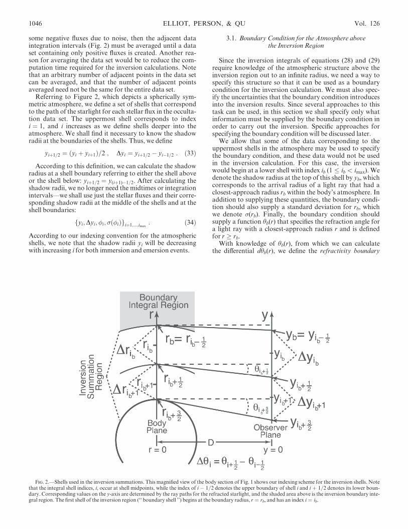
Referring to Figure 2, which depicts a spherically sym-metric atmosphere, we define a set of shells that correspondto the path of the starlight for each stellar flux in the occulta-tion data set. The uppermost shell corresponds to indexi = 1, and i increases as we define shells deeper into theatmosphere. We shall find it necessary to know the shadowradii at the boundaries of the shells. Thus, we define

yiþ1=2 ¼ ðyi þ yiþ1Þ=2 ; Dyi ¼ yiþ1=2 � yi�1=2 : ð33Þ

According to this definition, we can calculate the shadowradius at a shell boundary referring to either the shell aboveor the shell below: yi+1/2 = y(i+1)�1/2. After calculating theshadow radii, we no longer need the midtimes or integrationintervals—we shall use just the stellar fluxes and their corre-sponding shadow radii at the middle of the shells and at theshell boundaries:

fyi;Dyi; �i; ð�iÞgi¼1;...;imax: ð34Þ

According to our indexing convention for the atmosphericshells, we note that the shadow radii yi will be decreasingwith increasing i for both immersion and emersion events.

3.1. Boundary Condition for the Atmosphere abovethe Inversion Region

Since the inversion integrals of equations (28) and (29)require knowledge of the atmospheric structure above theinversion region out to an infinite radius, we need a way tospecify this structure so that it can be used as a boundarycondition for the inversion calculation. We must also spec-ify the uncertainties that the boundary condition introducesinto the inversion results. Since several approaches to thistask can be used, in this section we shall specify only whatinformation must be supplied by the boundary condition inorder to carry out the inversion. Specific approaches forspecifying the boundary condition will be discussed later.

We allow that some of the data corresponding to theuppermost shells in the atmosphere may be used to specifythe boundary condition, and these data would not be usedin the inversion calculation. For this case, the inversionwould begin at a lower shell with index ib (1 � ib < imax). Wedenote the shadow radius at the top of this shell by yb, whichcorresponds to the arrival radius of a light ray that had aclosest-approach radius rb within the body’s atmosphere. Inaddition to supplying these quantities, the boundary condi-tion should also supply a standard deviation for rb, whichwe denote (rb). Finally, the boundary condition shouldsupply a function hb(r) that specifies the refraction angle fora light ray with a closest-approach radius r and is definedfor r rb.

With knowledge of hb(r), from which we can calculatethe differential dhb(r), we define the refractivity boundary

Fig. 2.—Shells used in the inversion summations. This magnified view of the body section of Fig. 1 shows our indexing scheme for the inversion shells. Notethat the integral shell indices, i, occur at shell midpoints, while the index of i � 1/2 denotes the upper boundary of shell i and i + 1/2 denotes its lower boun-dary. Corresponding values on the y-axis are determined by the ray paths for the refracted starlight, and the shaded area above is the inversion boundary inte-gral region. The first shell of the inversion region (‘‘ boundary shell ’’) begins at the boundary radius, r = rb, and has an index i = ib.


integral,B�(rb, r), as follows:

B�ðrb; rÞ � � 1

�

Z �ðrbÞ

0

cosh�1

�r0

r

�d�bðr0Þ ; rb r : ð35Þ

We also define a pressure boundary integral, Bp(rb, r):

Bpðrb; rÞ

� � 1

�r

Z �ðrbÞ

0

�cosh�1

�r0

r

��


�r

r0

�2s �

d�bðr0Þ ;

rb r : ð36Þ

The boundary condition may also specify standard devia-tions for refractivity and pressure boundary integrals, whichwe denote (B�(rb, r)) and (Bp(rb, r)), respectively.

Next we define the refractivity integral, I�(rb, r), and thepressure integral, Ip(rb, r), over the region of atmospherebelow rb:

I�ðrb; rÞ � � 1

�

Z �ðrÞ

�ðrbÞcosh�1

�r0

r

�d�ðr0Þ ; rb r ; ð37Þ

Ipðrb; rÞ

� � 1

�r

Z �ðrÞ

�ðrbÞ

�cosh�1

�r0

r

��


�r

r0

�2s �

d�ðr0Þ ;

rb r : ð38Þ

With these definitions, we can rewrite the inversion integralsgiven by equations (28) and (29) as sums over the boundaryregion and the inversion region:

I�ðrÞ ¼ B�ðrb; rÞ þ I�ðrb; rÞ ; ð39ÞIpðrÞ ¼ Bpðrb; rÞ þ Ipðrb; rÞ : ð40Þ

3.2. Summation Equations for the Inversion Integrals

In this section we want to evaluate the inversion integrals,as given by equations (39) and (40). This requires us to relatethe observed stellar occultation fluxes to the radii andrefraction angles that appear in their integrands and toapproximate the integrals as sums over the atmosphericshells (Fig. 2). To begin this task, we rewrite equation (5) asthe sum of two integrals, one over the region of the atmo-sphere covered by the boundary condition and the otherover the region of the atmosphere covered by the inversion.We also reverse the limits of integration to match the orderof the anticipated summation, from higher to lower radii:

r¼�y2 � 2

Z y

yb

½1� �ðy0Þ�y0 dy0 � 2

Z yb

1½1� �ðy0Þ�y0 dy0

�1=2

:

ð41Þ

Next we note that the radius for the boundary of theinversion, rb, is given by the equation

r2b ¼ y2b � 2

Z yb

1½1� �ðy0Þ�y0 dy0 : ð42Þ

Substituting equation (42) into equation (41) and integrat-ing the constant term, we find the following expression for r:

r ¼�r2b þ 2

Z y

yb

�ðy0Þy0 dy0�1=2

: ð43Þ

In order to evaluate equation (43) as a sum over fluxes andshadow radii, we first write the sum that approximates theintegral of equation (43) for calculating the body radius atthe shell boundaries ri+1/2 (for i ib):

riþ1=2 ¼�r2b þ 2

Xi

j¼ib

�jyj Dyj

�1=2

: ð44Þ

We can now define the radius increments for the ith shell,Dri, as the differences between their values at the shellboundaries (for i ib):

Dri ¼ riþ1=2 � ri�1=2 : ð45Þ

The radius for the middle of each shell is defined as theaverage of the radii at the shell boundaries:

ri ¼ðriþ1=2 þ ri�1=2Þ=2 ; if i > ib ;

ðriþ1=2 þ rbÞ=2 ; if i ¼ ib :

(ð46Þ

Approximating the distanceD between the observer and theocculting body as being constant, we can write an expres-sion for the refraction angle at the shell boundaries, hi�1/2,as a function of the observer-plane and sky-plane radii,yi�1/2 and ri�1/2:

�i�1=2 ¼ ðyi�1=2 � ri�1=2Þ=D : ð47Þ

We define Dhi for the ith shell as the difference between therefraction angle at the shell boundaries:

D�i � �iþ1=2 � �i�1=2 ¼ ðDyi � DriÞ=D : ð48Þ

Before writing equations approximating the inversionsums, we note that if the data represented by equation (32)are averaged in equal time intervals, then as the stellar fluxsteadily decreases, the radii within the atmosphere foundfrom equation (44) will become closer and closer together. Ifone wishes to maintain an approximately equal spacing forthe inversion results at some shell thickness Dr (Fig. 2)within the atmosphere of the occulting body, one can thenchoose a subset of the ri+1/2 for which consecutive valuesdiffer by an amount as close to the desired spacing as possi-ble. Corresponding values for yi, Dyi, �i, (�i), hi, Dhi, and riare also obtained for later use. In the equations that follow,we shall use the index i to refer to a contiguous set of ri+1/2,ri, and Dhi—whether they be the original set or a subset thathas been reindexed so that the i represents a continuous setof integers.

We now write an equation for the sums that approximatethe part of the inversion integrals (eqs. [37] and [38]) thatinclude the inversion region, which, in the limit of smallincrements of refraction angle, would converge to thedesired integrals:

I�ðrb; rÞ � 1

�

Xi

j¼ib

cosh�1

�rj

riþ1=2

�D�j ; ð49Þ


Ipðrb; rÞ � 1

�riþ1=2

Xi

j¼ib

�cosh�1

�rj

riþ1=2

�

�

ffiffiffiffiffiffiffiffiffiffiffiffiffiffiffiffiffiffiffiffiffiffiffiffiffiffiffiffiffiffi1�

�riþ1=2

rj

�2s �

D�j : ð50Þ

However, real data cannot be subdivided more finely thanthe original integration intervals, and we want the approxi-mation to the integrals to converge as well as possible for theintegration interval available. Hence, we follow the proce-dure of French et al. (1978) and integrate the functions of rin equations (49) and (50) before summing, since these func-tions change quickly near rj/ri+1/2 = 1.We define the ratios

zj� �rj�1=2

riþ1=2; zjþ �

rjþ1=2

riþ1=2: ð51Þ

Then we integrate the functions of r in equations (49) and(50) and define the sums S�(ib, ri+1/2) and Sp(ib, ri+1/2),which will approximate the inversion integrals somewhatbetter than those indicated in equations (49) and (50) forequal-sized inversion shells (Figs. 1 and 2):

S�ðrb; riþ1=2Þ � � 1

�

Xi

j¼ib

1

zjþ � zj�

� ½z cosh�1 z�ffiffiffiffiffiffiffiffiffiffiffiffiffiz2 � 1

p�zjþzj�D�j ;

ð52Þ

Spðrb; riþ1=2Þ � � 1

�

Xi

j¼ib

1

zjþ � zj�

� ½z cosh�1 z� 2ffiffiffiffiffiffiffiffiffiffiffiffiffiz2 � 1

p� sin�1 z�zjþzj�D�j :

ð53Þ

The equations for the refractivity, number density, pres-sure, temperature, and scale height at the lower boundary ofeach atmospheric shell within the inversion region can nowbe written in terms of the boundary integrals given byequations (35) and (36) and the summations given byequations (52) and (53):

�iþ1=2 � �ðrb; riþ1=2Þ ¼ B�ðrb; riþ1=2Þ þ S�ðib; riþ1=2Þ ; ð54Þ

niþ1=2 � nðrb; riþ1=2Þ ¼L

�STP�ðrb; riþ1=2Þ ; ð55Þ

piþ1=2 � pðrb; riþ1=2Þ

¼ lmamuLGMp

�STP½Bpðrb; riþ1=2Þ þ Spðib; riþ1=2Þ� ; ð56Þ

Tiþ1=2 � Tðrb; riþ1=2Þ ¼pðrb; riþ1=2Þknðrb; riþ1=2Þ

¼lmamuGMp½Bpðrb; riþ1=2Þ þ Spðib; riþ1=2Þ�

k½B�ðrb; riþ1=2Þ þ S�ðib; riþ1=2Þ�; ð57Þ

Hiþ1=2 � Hðrb; riþ1=2Þ

¼r2iþ1=2½Bpðrb; riþ1=2Þ þ Spðib; riþ1=2Þ�

B�ðrb; riþ1=2Þ þ S�ðib; riþ1=2Þ: ð58Þ

3.3. A Specific Boundary Condition

As discussed earlier, the boundary condition for theinversion must specify a boundary radius rb at which

the inversion summations begin. It also must specify therefraction angle hb(r) and its differential dhb(r) for radiigreater than rb. Although there is some latitude in estab-lishing the boundary condition, the value of rb and thesefunctions are not completely arbitrary, in that theyshould reproduce the light curve corresponding to radiiabove rb as closely as possible. For example, the chosenvalue of rb should satisfy equation (5) both for theactual light curve and the synthetic light curve generatedfrom the functions hb(r) and dhb(r) supplied by theboundary condition. Also, any additional parameters ofthe boundary condition should be adjusted so that thesynthetic light curve generated from the boundary con-dition matches the actual light curve as closely aspossible.

One approach for achieving a close relationshipbetween the boundary condition and the actual lightcurve corresponding to radii greater than rb is to first fita model to this portion of the light curve and then usethe fitted model to determine rb and the refraction-anglefunction and its differential function. One such model,appropriate for Pluto and Triton, is that of Paper I,which allows a possible thermal gradient in the atmo-sphere. Paper I used a power-law dependence of temper-ature with radius, not for physical reasons but becausethis functional form allows a thermal gradient withfewer mathematical difficulties in generating a syntheticlight curve than other functional forms considered. Ifwe specify the half-light radius rh as the reference radiusand set the temperature here as Th, then the temperatureas a function of radius, T(r), is determined by a powerindex b:

TðrÞ ¼ Thðr=rhÞb ð59Þ

(Paper I). In Paper I, the half-light radius is defined asthe radius within the body’s atmosphere that corre-sponds to a normalized stellar flux of 0.5 in theobserver plane, including the effects of differentialrefraction and lateral focusing (but not extinction).

The model in Paper I also allows a power-law dependenceof the mean molecular weight as a function of radius, but weshall not use that generality here. Hence we set the power-law index a for molecular weight variation equal to zerowhen using the equations in Paper I.

The temperature at half-light is most easily related to thelight curve through an intermediate parameter h that is theratio of gravitational potential energy to kTh. The value ofTh can be determined from h, rh, and other physicalconstants:

Th ¼lmamuGMp

khrhð60Þ

(Paper I). For a bound atmosphere, h 4 1 (e.g., h � 3000for Jupiter,�60 for Triton, and�20 for Pluto). Also, as dis-cussed in Paper I, h = rh/Hh, whereHh is the pressure scaleheight at half-light, and (r) = h(r/rh)

�(1+b).We can now write an equation for (r), using its

definition and equation (59):

ðrÞ � lmamuGMp

rkTðrÞ ¼ hr

rh

� ��ð1þbÞ: ð61Þ


According to the fitting procedure recommended inPaper I, the ‘‘ equivalent isothermal ’’ lambda, hi, is fitfor instead of h because it is less correlated with thepower index b. The two energy ratios are related byequation (5.13) in Paper I, which we repeat here (settinga = 0):

h ¼ hi � 5b=2 : ð62Þ

Hence, as the result of fitting the appropriate portion ofa light curve to establish the boundary condition, wedetermine the parameters h, rh, and b that describe theatmosphere within the boundary region.

We now use these parameters to find the requiredfunctions for the refraction angle, its derivative, and theboundary radius for the inversion, rb. First we write anequation for the refraction angle within the boundary,hb(r) (given by eq. [4.6] of Paper I). We use a slightlydifferent notation from that of Paper I to emphasize ther-dependence:

�bðrÞ ¼ �ffiffiffiffiffiffiffiffiffiffiffiffiffiffi2�ðrÞ

p�ðrÞAðr; bÞ : ð63Þ

In equation (63), the function A(r, b) is an asymptoticpower series in the parameters b and r [found by settingthe parameter a = 0 in eq. (A2) in Paper I, which hasan erroneous coefficient of the b3�4(r) term that hasbeen corrected here]:

Aðr;bÞ ¼ 1� 3� 3b

8�1ðrÞ � 15� 14b� b2

128�2ðrÞ

� 105� 27b� 69b2 � 9b3

1024�3ðrÞ

� 4725þ 4236b� 4706b2 � 3764b3 � 491b4

32768�4ðrÞ

þ � � � : ð64Þ

The refractivity, �(r), is given in terms of the refractivityat half-light �h and previously defined quantities:

�ðrÞ ¼ �h

�r

rh

�b

exp

�ðrÞ � h

1þ b

�: ð65Þ

For b = 0 and for the approximation of constant gravi-tational acceleration, the right-hand side of equation (65)reduces to the familiar form �h exp [�(r � rh)/Hh], whereHh is the pressure scale height (Paper I). Equation (4.28)of Paper I gives an expression for �h:

�h ¼rh

2Dffiffiffiffiffiffiffiffiffiffi2�h

p�1� 1

hBðrh;bÞ

�ffiffiffiffiffiffiffiffiffiffiffiffiffiffiffiffiffiffiffiffiffiffiffiffiffiffiffiffiffiffiffiffiffiffiffiffiffiffiffiffiffiffiffiffiffiffiffiffiffiffiffiffiffiffiffi1� 6

hBðrh;bÞþ 1

2hBðrh;bÞ

2

s �: ð66Þ

To evaluate equation (66), we need an expression forthe asymptotic power series, B(r, b), which can be foundby evaluating equation (A5) in Paper I with theparameter a set to zero. An erroneous coefficient of theb2�4(r) term in Paper I has been corrected, and weuse a slightly different notation to emphasize the

r-dependence:

Bðr;bÞ ¼ 1þ 1þ 15b

8�1ðrÞ þ 9� 34bþ 25b2

128�2ðrÞ

þ 75� 81bþ b2 þ 5b3

1024�3ðrÞ

þ 3675� 1356b� 2110b2 � 268b3 þ 59b4

32768�4ðrÞ

þ � � � : ð67Þ

Having all the information needed to calculate therefraction angle, we iteratively solve the equation belowto find rb in terms of the fitted model parameters andyb:

rb ¼ yb �D�bðrbÞ : ð68Þ

Finally, we write the equation for the differential of therefraction angle, as given by equation (4.9) of Paper I:

d�bðrÞ ¼ffiffiffiffiffiffiffiffiffiffiffiffiffiffiffiffi2�ðrÞ3

q�ðrÞr

Bðr;bÞdr : ð69Þ

This completes our specification of the boundary condi-tion for the power-law thermal model of Paper I, whichis summarized by equations (63), (68), and (69).

4. EVALUATION OF ERRORS IN THEINVERSION RESULTS

In this section we shall evaluate the random errors in theradius scale, refractivity, number density, pressure, temper-ature, and scale height that arise from the random errors inthe fluxes, (�i). Errors arising from other causes will be dis-cussed in x 7.4. In the first subsection, x 4.1, we consider therandom errors that arise from the boundary condition andprovide a general method for combining these with thosefrom the inversion summations. Specific equations forapplying this method to each of the atmospheric quantitiesof interest are given in subsequent subsections.

4.1. Combining Errors from the Boundary Conditionand Inversion Sums

The parameters describing the boundary condition willintroduce errors into the results of the inversion in a mannerthat will depend on how the boundary condition is specified.If we use the boundary condition specified in x 3.3, which isa least-squares fit of a model to the portion of the light curvethat lies outside the inversion sums, then the boundary con-tribution to the errors in the inversion is straightforward.One class of boundary conditions includes those withparameters determined from a least-squares fit to the por-tion of the light curve that corresponds to the atmosphereabove the boundary. For this class, we assume that we havea function f that can have arguments that do not have ran-dom errors (i.e., not included as fitted parameters). Thefunction also has arguments q1, . . . , qN that are fitted (whichwe shall refer to as the boundary parameters), and the jthand kth parameters have a covariance, Cov (qj, qk). Thecovariances are determined by the least-squares fit(Bevington & Robinson 1992). Alternatively, we can definethe correlation coefficient, �jk, in terms of the covariances


and standard deviations, (qj) and (qk), of the boundaryparameters with the following equation:

�jk ¼ Cov ðqj; qkÞðqjÞðqkÞ

: ð70Þ

The standard deviation of f, ( f ), is then given by theequation

ð f Þ ¼�XN

j¼1

XNk¼1

@f

@qj

@f

@qk�jkðqjÞðqkÞ

�1=2: ð71Þ

For the example in x 3.3, the fitted parameters are hi, rh,and b. With knowledge of these, the quantities needed tocalculate the boundary conditions for the inversion can beobtained, working backward from equations (63), (68), and(69).

We now note that all quantities determined from theinversion (including the boundary condition) can be calcu-lated from the boundary parameters q1, . . . , qN. These con-solidate the relevant information contained in the fluxes{’i}i¼1;...;ib�1 that passed through the atmosphere above theboundary. As the fluxes remaining in the light curve (thosepassing through the atmosphere below the boundary,{’i}i¼ib;...;imax

) were not used in establishing the boundarycondition, they are uncorrelated with the boundaryparameters, for we have already stipulated that the fluxesare uncorrelated with each other.

Knowing the error for each uncorrelated parameter,including the fluxes, we can calculate the error for any quan-tity associated with the ith atmospheric shell, xi (or xi+1/2),with the usual methods of error propagation (Bevington &Robinson 1992). We define �(xi) to be an operator that canbe used to generate the standard deviation of the calculatedquantity xi. It is given by the equation

�ðxiÞ ��XN

j¼1

XNk¼1

@xi@qj

@xi@qk

�jkðqjÞðqkÞ

þXi

k¼ib

�@xi@�k

�2

2ð�kÞ�1=2

: ð72Þ

We shall use equation (72) as the basis for calculating theerror for the radius scale and all atmospheric quantitiesderived from the inversion.

4.2. Errors in the Radius Scale

To calculate the error in the radius scale, we begin withthe first term on the right-hand side of equation (72), whichcorresponds to the error contribution from the region of thelight curve included in the boundary condition. For thiscase, the information from the fitted parameters (hi, rh, andb) for our example boundary condition can be consolidatedinto a single parameter, rb. Hence we can write equation (72)for the standard deviation of ri+1/2 by using the definition ofri+1/2 given by equation (44):

ðriþ1=2Þ ¼ �ðriþ1=2Þ ¼��

@riþ1=2

@rb

�2

2ðrbÞ

þXi

k¼ib

�@riþ1=2

@�k

�2

2ð�kÞ�1=2

: ð73Þ

Again using equation (44), we determine the partial deriva-tives required by the right-hand side of equation (73):

@riþ1=2

@rb¼ rb

riþ1=2; ð74Þ

@riþ1=2

@�k¼

yk Dyk=riþ1=2 ; if ib � k � i ;

0 ; otherwise :

�ð75Þ

Substituting these derivatives into equation (73), we find

ðriþ1=2Þ ¼1

riþ1=2

�r2b

2ðrbÞ þXi

k¼ib

y2k Dy2k

2ð�kÞ�1=2

: ð76Þ

In this result, we determine rb and (rb) from the boundarycondition—using equation (71)—and the yk are found fromthe geometric solution for the occultation. The latter shouldhave negligible errors.

We square equation (76) and define two quantities thatwe shall find useful later. We define 2

q;r as the contributionto the variance in ri+1/2 arising from the boundary conditionand 2

�;r as the contribution to the variance in ri+1/2 arisingfrom the flux summation terms in the inversion:

2q;r � r2b

2ðrbÞ=r2iþ1=2 ; ð77Þ

2�;r � ½

Xi

k¼iby2k Dy

2k

2ð�kÞ�=r2iþ1=2 : ð78Þ

Thus, equation (76) can be rewritten as follows:

ðrÞ ¼ffiffiffiffiffiffiffiffiffiffiffiffiffiffiffiffiffiffiffiffi2q;r þ 2

�;r

q: ð79Þ

4.3. Errors in Refractivity and Number Density

To generate an expression for the rms errors in the refrac-tivity and number density, we apply equation (72) to equa-tion (54). Our equations will be more compact here andin the following sections if we make the definitionsB� � B�(rb, ri+1/2), Bp � Bp(rb, ri+1/2), S� � S�(rb, ri+1/2),and Sp � Sp(rb, ri+1/2). With this notation, we write theequation for the rms error in the refractivity as

ð�iþ1=2Þ ¼ �ðB� þ S�Þ : ð80Þ

The error in the number density is proportional to the errorin refractivity:

ðniþ1=2Þ ¼L

�STPð�iþ1=2Þ : ð81Þ

Evaluation of the boundary parameter term in equation (80)is a straightforward application of equation (71):

2q;� ¼

XNj¼1

XNk¼1

�@B�

@qjþ @S�

@qj

��@B�

@qkþ @S�

@qk

��jkðqjÞðqkÞ :

ð82Þ

To evaluate the summation part, we need the partial deriva-tives that appear in the second term on the right-hand sideof equation (72), which we evaluate numerically to find thevariance of S�:

2�;� ¼

Xi

k¼ib

�@B�

@�kþ @S�

@�k

�2

2ð�kÞ : ð83Þ


Finally, we write the final result for the rms error in therefractivity, which can be evaluated with equations (82) and(83):

ð�iþ1=2Þ ¼ffiffiffiffiffiffiffiffiffiffiffiffiffiffiffiffiffiffiffiffiffi2q;� þ 2

�;�

q: ð84Þ

4.4. Errors in the Pressure

Evaluation of the rms error in the pressure followsequations that are completely analogous to those for therefractivity, beginning with equation (80):

ðpiþ1=2Þ ¼lmamuLGMp

�STP�ðBp þ SpÞ ; ð85Þ

2q;p ¼

XNj¼1

XNk¼1

�@Bp

@qjþ @Sp

@qj

��@Bp

@qkþ @Sp

@qk

��jkðpjÞðpkÞ ;

ð86Þ

2�;p ¼

Xi

k¼ib

�@Bp

@�kþ @Sp

@�k

�2

2ð�kÞ ; ð87Þ

ðpiþ1=2Þ ¼ffiffiffiffiffiffiffiffiffiffiffiffiffiffiffiffiffiffiffiffiffi2q;p þ 2

�;p

q: ð88Þ

4.5. Errors in the Temperature

Equations for the random errors in the temperature aremore complex than those for refractivity and pressure, sincethe temperature involves a ratio of quantities derived fromrandom variables. We begin by writing the rms error for thetemperature with equation (72):

ðTiþ1=2Þ ¼lmamuGMp

k

� �

�Bpðrb; riþ1=2Þ þ Spðib; riþ1=2ÞB�ðrb; riþ1=2Þ þ S�ðib; riþ1=2Þ

�: ð89Þ

Next we continue the calculation by finding the contribu-tion to the variance in the temperature that arises from theboundary parameters, 2

q;T , and the contribution to thevariance in the temperature that arises from the errors inthe fluxes, 2

�;T . First we write the expression for 2q;T by

applying equation (71):

2q;T ¼ 1

ðB� þ S�Þ4

�XNj¼1

XNk¼1

�ðB� þ S�Þ

�@Bp

@qjþ @Sp

@qj

�

� ðBp þ SpÞ�@B�

@qjþ @S�

@qj

��

��ðB� þ S�Þ

�@Bp

@qkþ @Sp

@qk

�


@qkþ @S�

@qk

��jkðqjÞðqkÞ :

ð90Þ

We note that all quantities needed to evaluate equation (90)have appeared previously. Next we write an equation for

2�;T , again noting that all quantities in the equation have

appeared previously:

2�;T ¼ 1

ðB� þ S�Þ4

�Xi

k¼ib

�ðB� þ S�Þ

�@Bp

@�kþ @Sp

@�k

�


@�kþ @S�

@�k

��22ð�kÞ : ð91Þ

Finally, we write the equation for the desired result, whichcan be evaluated with the aid of equations (90) and (91):

ðTiþ1=2Þ ¼lmamuGMp

k

ffiffiffiffiffiffiffiffiffiffiffiffiffiffiffiffiffiffiffiffiffiffiffi2q;T þ 2

�;T

q: ð92Þ

4.6. Errors in the Scale Height

We derive an expression for the rms error in the scaleheight, again beginning with equation (72):

ðHiþ1=2Þ ¼ �

�r2iþ1=2

Bp þ Sp

B� þ S�

�: ð93Þ

Here we have a situation similar to the calculation of thetemperature error in the previous subsection, except for theadded complication of the multiplicative factor r2iþ1=2. Weapproach the calculation in the same way as we did forthe temperature, first finding the contribution to the var-iance of the scale height, 2(Hi+1/2), that arises from theboundary parameters, 2

q;H , and then finding the contribu-tion to the variance that arises from the summation of theflux terms in the inversion, 2

�;H . In this case the error inri+1/2 has contributions from both the boundary parametersand the inversion fluxes, so it must be included in both theboundary and summation variances.

First we write the equation for the contribution to thevariance arising from the boundary parameters:

2q;H ¼ 1

ðB� þ S�Þ4

�XNj¼1

XNk¼1

�ðB� þ S�Þ

�r2iþ1=2

�@Bp

@qjþ @Sp

@qj

�

þ ðBp þ SpÞ@r2iþ1=2

@qj

�

� r2iþ1=2ðBp þ SpÞ�@B�

@qjþ @S�

@qj

��

��ðB� þ S�Þ

�r2iþ1=2

�@Bp

@qkþ @Sp

@qk

�


@qk

�

� r2iþ1=2ðBp þ SpÞ�@B�

@qkþ @S�

@qk

�� jkðqjÞðqkÞ: ð94Þ

Next we write an equation for the contribution to thevariance arising from the summation in fluxes, keeping the


r2iþ1=2 factor grouped with the pressure summation term:

2�;H ¼ 1

ðB� þ S�Þ4

�Xi

k¼ib

�ðB� þ S�Þ

�r2iþ1=2

@ðBp þ SpÞ@�k


@�k

�

� r2iþ1=2ðBp þ SpÞ@ðB� þ S�Þ

@�k

�2

2ð�kÞ :

ð95Þ

Two derivatives in equation (95) require evaluation:

@r2iþ1=2Sp

@�k¼ r2iþ1=2

@Sp

@�kþ 2riþ1=2Sp

@riþ1=2

@�k

¼ r2iþ1=2

@Sp

@�kþ 2yk DykSp ; ð96Þ

@r2iþ1=2

@�k¼ 2riþ1=2

@riþ1=2

@�k¼ 2yk Dyk ; ð97Þ

where the flux derivative for ri+1/2 is given by equation (75).Finally, we write the desired error in scale height as thesquare root of the sum of the variances given byequations (94) and (95):

ðHiþ1=2Þ ¼ffiffiffiffiffiffiffiffiffiffiffiffiffiffiffiffiffiffiffiffiffiffiffiffi2q;H þ 2

�;H

q: ð98Þ

5. NUMERICAL EVALUATION OF THEINVERSION INTEGRALS

In order to provide a standard, trustworthy, and repeat-able procedure for the calculations described by ourequations, we designed and implemented a set of functionsand a template using the program Mathematica 4.0(Wolfram 1999). Each function implements equations orparts of equations from this paper. The template then usesthese functions and the data provided by the user to performthe desired inversion calculations.

Numerical evaluation of the inversion requires inputs ofvarious types. First, there are the physical parameters suchas distance, mass, composition of the body’s atmosphere,and the physical constants needed to calculate pressure,density, and temperature. Second, we need a set of parame-ters that specify the atmospheric structure within the boun-dary region. Third, we need the normalized stellar fluxes{�i}, their errors {(�i)}, and their corresponding coordi-nates in the observer plane {yi}. Finally, two parameters forthe inversion calculations must be provided: (1) the (mini-mum) shell thickness and (2) the position in the list of nor-malized stellar fluxes that specifies the transition from theboundary region to the inversion region (Fig. 2). Althoughthe fluxes are normalized, some may still be less than zerobecause of noise in the data. Therefore, we average any neg-ative flux with the flux or fluxes that follow until all the finalaveraged fluxes are positive. Mid-y’s and flux errors are thengenerated to correspond to these averaged flux values. Asmentioned in x 3, we may choose to reduce the resolution of

the data by averaging several flux, flux error, and mid-ypoints. This and the procedure to obtain positive flux maybe performed in either order. We have chosen to reduce theresolution first, because the reduction in data resolutionmay remove some negative flux values (or eliminate thementirely).

The calculations take place in several steps. First weperform a least-squares fit with the mid-y’s, fluxes, andflux errors above the boundary to determine the boun-dary model parameters and their errors. Next we usethese fitted parameters and other values to calculate thevalues of y, radius, and theta at the boundary (yb, rb, hb).Then we use the mid-y’s, fluxes, flux errors below theboundary, and delta y’s (Dyi)—calculated from equations(41) through (48)—to calculate the lower boundary radii,mid-radii, delta radii, lower boundary theta, and deltatheta (ri+1/2, ri, Dr, hi+1/2, Dh). The next step is to com-bine the adjacent data as necessary so that the delta radiiare (the minimum amount) larger then the specified mini-mum shell thickness. Finally, we use these data lists tocalculate the refractivity, density, pressure, temperature,and scale height with equations (54) through (58) andtheir errors with equations (76) through (98). Thiscalculation flow is diagrammed in Figure 3.

In calculating the errors, we found that—except for theradii—analytical derivatives are difficult to derive andimplement. Therefore, those derivatives are calculatednumerically (as one-sided finite differences, to save compu-tation time). We wrote one set of generic numerical deriva-tive and variance functions for the boundary terms andanother set for the summation terms. These two sets of func-tions together correspond to equation (72). For the boun-dary terms, each fitted parameter is individually stepped by1/10 of its formal error, and the resulting derivatives arecombined with the errors and the correlation matrix toreturn the variance. For the summation terms, we individu-ally stepped each flux by a tenth of its error, and then werecalculated the lower boundary radii, mid-radii, deltatheta, etc., from these stepped fluxes and the correspondingy’s to find the variances. It is important to note the inter-mediate results that are calculated from the fitted boundaryparameters and fluxes and to make sure that all these inter-mediate results are recalculated with the stepped values ofthe fluxes.

After calculating the atmospheric profiles and theirerrors, standard plots and tables are generated to displaythe results, and the template ‘‘ notebook ’’ writes theseresults to a file for future use.

6. TESTS WITH SYNTHETIC LIGHT CURVES

In order to test the reliability of our method, we carriedout inversions on a set of synthetic light curves. Our objec-tive was to examine how the inversion temperature profileschanged for model occultation light curves similar to thoseof Triton and Pluto when we varied the (1) boundary radius,(2) data-averaging interval, (3) atmospheric shell thickness(Fig. 2), (4) thermal gradient in the occulting body’s atmo-sphere, (5) level of light-curve noise, and (6) backgroundlevel (by introducing systematic errors into the zero stellarflux level).

We note that our method presents three opportunities foraveraging or binning the data and the intermediate results.First, the stellar fluxes can be averaged in the time domain


prior to constructing the data set represented by equation(32). Secondly, the data set represented by equation (32) canbe averaged further after being transformed from a functionof time to a function of the y-coordinate in the observerplane. Finally, after using the fluxes to construct the atmo-spheric shells with equations (44) through (48), the adjacentshells can be binned into thicker shells if desired.

6.1. Reference Point and Scaling of the Test Results

A common reference point within the occulting body’s at-mosphere for occultation results is the radius of half-light(x 3.3 and Paper I), and the widely used distance scale is thepressure scale height (Paper I). Regardless of the absoluteradius interval within the occulting body’s atmosphere

Fig. 3.—Flowchart for the inversion calculation. Calculation generally flows from left to right, as the initial data, represented by eq. (32), are processed tothe complete inversion profiles on the right. Note the recurrence of certain key equations, such as eq. (72), which appears as part of the error calculations ineach segment of the output.


covered by the inversion, or the actual radius range coveredby individual data points, the parameter that controls therate at which various errors grow is the number of scaleheights relative to the reference point. Tests conducted byrescaling all parameters resulting from changing the scaleheight indeed give virtually identical results. Hence, we haveadded a ‘‘ scale heights above half-light ’’ scale to our plots(along with the radius scale) to facilitate scaling our testresults to other cases of interest.

Also, as will be discussed in x 6.3, the errors in the quanti-ties determined by the inversion scale inversely with thesignal-to-noise ratio (per scale height interval) of theoccultation light curve. This can be seen in equation (72),where the variance of the stellar fluxes is a multiplier in thesecond summation term. The same scaling applies tothe first (double) summation term in equation (72), whenthe data are accurate enough for the linear approximationfor the least-squares fitting of a nonlinear light-curve modelto be valid. This is almost always the case.

6.2. Tests with Noiseless Synthetic Light Curves

6.2.1. Standard Test Case

A standard test case was established to confirm the basicaccuracy of the method in reproducing an expected thermalprofile. The Paper I small-body atmospheric model wasused to generate the standard test-case data. The model at-mosphere for the standard case is isothermal (i.e., b = 0)with a temperature of 80 K, a 30 AU body-observer dis-tance, a pressure scale height (at half-light) of 30 km, and ahalf-light radius of 1200 km. The full resolution of the data(Dy = 0.5 km per data point) was used, and the resultingDr’s were binned to a minimum shell size of 1.0 km. A com-plete tabulation of the parameters used to generate thelight-curve data from the Paper I model is given in Table 1.

A limitation of our standard test case is that the modelused to generate the synthetic light curve for our tests is notexact but involves asymptotic series expansions that canbe carried out to different orders (see Paper I). In orderto understand the limitation that our light-curve model

imposes on our inversion testing, we generated light curveswith different orders of the asymptotic series and invertedthem. Figure 4 shows these results. In the top panel, we see alarge improvement in the accuracy of the light curve byusing just the first term of the series. In the greatly expandedscale of the bottom panel, we see further improvement if theseries order is increased to 2, but not much improvementbeyond that. Hence we elected to use a series expansionorder of 2 for our standard test case. This case is plotted as aheavy line in the top and bottom panels of Figure 4, as wellas in the remaining test-case figures.

The remaining differences from an isothermal tempera-ture are due to a combination of (1) limitations in thenumerical inversion process (most notably the approxima-tion of integrals by sums), (2) errors in the synthetic data asgenerated from the Paper I model, and (3) possible (small)systematic errors due to the one-sided (rather than two-sided) numerical derivatives. If desired, the second effectcould be eliminated by inverting a sample light curve gener-ated from an exact analytical solution to a known thermalprofile (Eshleman & Gurrola 1993; Chamberlain & Elliot1997), and the third effect could be eliminated with the useof two-sided derivatives (at some expense of computationtime). However, the errors in our standard test case are wellbelow 0.01% and not important for practical purposes: inthe bottom panel of Figure 4 we see that the inversion accu-rately reproduces the 80 K isothermal profile of the modelatmosphere within 0.01 K. The average temperature givenby all points of the inverted profile is 79.997 K, very close tothe model value, although the final points of the inversionconverge to a slightly closer value of 79.998 K.

6.2.2. Isothermal Tests

Variations of the inversion parameters from their val-ues in this standard case were carried out with the samedata as used in the standard case. Each parameter waschanged independently, with the values for the otherparameters kept at their values in the standard case.Table 2 gives the values used in the trial inversions forsynthetic light curves that were calculated with the

TABLE 1

Parameters Used for the Standard Test Case

Parameter Value Explanation

Explicit model parameters:

rh (km).................................................. 1200 Half-light radius of occulting atmosphere

Th (K)................................................... 80 Temperature of occulting atmosphere at half-light

h ......................................................... 40 Energy ratio at half-light (Paper I)

b ........................................................... 0 Exponent of temperature gradient in occulting atmosphere (isothermal for b = 0)

Distance (AU)...................................... 30 Distance between occulting body and observer

Atmospheric composition .................... N2

Meanmolecular weight (amu) .............. 28.01

Refractivity at STP (�10�4).................. 2.98

Derivedmodel parameters:

Mass (kg) ............................................. 1.70833 � 1022 Mass of occulting body

Scale height at half-light (km)............... 30

Inversion parameters:

Order ................................................... 2 Order of asymptotic series expansions in boundarymodel calculations (Paper I)

Radial resolution,Dy (km) ................... 0.5 Resolution of synthetic data in observer plane

Shell thickness, Dr (km) ........................ 1.0 Minimum thickness of inversion shells in occulting body’s atmosphere

Flux level at boundary index ................ 0.5 Stellar flux level at which inversion begins

Points in the boundary region............... 860

Points in the inversion region................ 80


small-body model described in Paper I, where the param-eter values for the standard test case are displayed inboldface. All columns but the last refer to parameter var-iations used with noiseless light curves. Each value in thetable indicates one inversion trial in which the tabulatedparameter was fixed as given, with all other parametersset to their standard values.

The three panels in Figure 5 show the temperature pro-files used to characterize the sensitivity of the inversionresults to (1) different stellar flux levels used to specifythe inversion boundary (which effectively specify theinversion boundary radius, rb) (2) different averagingintervals of the data in the observer plane (y-coordinate),and (3) different minimum shell sizes within the occultingbody’s atmosphere (r-coordinate). As seen in the toppanel, changing the value of the boundary flux producesonly a small error in the resulting temperature—muchless than 0.01% for all cases considered. In the next setof test cases (Fig. 5, middle), we averaged the data overdifferent intervals in the observer plane, which we haveexpressed in terms of ‘‘ points per scale height ’’ for theaveraged data. The extreme case for this test was to aver-age the data over 30 km intervals. Although this distanceequals 1 scale height of the occulting body’s atmosphere,the actual interval sampled within the occulting body’satmosphere is only 15 km at half-light—because of differ-ential refraction—and the corresponding distance withinthe occulting body’s atmosphere becomes progressivelyless as the stellar flux decreases (see eq. [2]). Even foraveraging the data to one point per scale height (in theobserver plane), the maximum error in the temperatureprofile resulting from the inversion is less than 0.5%.

A different way to average the data is to bin the atmo-spheric shells, and the effects of this procedure are illustratedin the bottom panel of Figure 5. As with averaging the datain the observer plane, the temperature errors are small andreach a maximum error of less than 0.7% for a binningof two points per scale height. This extreme binningcorresponds to 15 km (half a scale height) in the body’satmosphere.

Table 3 gives the representative values of average tem-perature inverted and final convergence temperature forselected inversion test cases just described. For all cases, theactual temperature is the standard value of 80 K. The

Fig. 4.—Isothermal test cases: different orders for series expansions. Thisfigure displays the results of inversions of the standard test case for differentorders of the asymptotic series expansion (eqs. [64] and [67] in x 3.3) for thelight-curve model (Paper I) used for these tests. Both panels show a plot oftemperature (abscissa) vs. radius (ordinate). The right ordinate scale showsthe scale heights above half-light equivalent to the radius scale on the left,and the top scale represents the percentage deviation of the calculatedtemperature from the model temperature of 80 K (shaded vertical line).Different line styles have been plotted instead of discrete temperature pointsto make the results for different inversions more distinguishable. The heavysolid line represents the standard isothermal test case in both panels. Thebottom panel gives an expanded view of the left portion of the top panel,which illustrates the difference of the temperature profile for the first-orderexpansion from that for the second-order expansion (standard test case).The curves for the third- and fourth-order results are nearly indistin-guishable from the second-order result. Note the extremely expandedtemperature scale of the bottom panel.

TABLE 2

Parameters for Test Cases

Inversion Trial

Series

Series Expansion

Order

Data Resolution,a y

(km)

Shell Size,aDr

(km)

Flux at Boundary

Radius

Thermal Gradient

Parameter, b

Signal-to-Noise

Ratio, (S/N)Hb

1............................ 0 0.5 1 0.3 �6 11112............................ 1 1 2 0.4 �3 500

3............................ 2 2 6 0.5 0 200

4............................ 3 3 12 0.6 3 100

5............................ 4 5 20 0.7 6 50

6............................ . . . 10 30 0.8 9 20

7............................ . . . 30 . . . . . . . . . . . .8............................ . . . 60 . . . . . . . . . . . .

Note.—Each tabulated value represents a single trial, and parameters for the standard test case are in boldface. For that trial, the tabulated valuewas fixed as listed and all other values were fixed to their value for the standard case given in boldface. The series expansion order refers to eqs. (64) and(67) describing the model, and the thermal gradient parameter b refers to eq. (59) (see Paper I).

a Scale height is 30 km.b Background-limited.


inversion procedure yields remarkably accurate tempera-tures, even when the data are averaged over large intervalsin the observer plane or the atmospheric shells have beenbinned to a thickness of half a scale height.

6.2.3. Nonisothermal Tests

In order to ensure that our results are applicable to awider set of data than the isothermal test cases establishabove, we inverted a test series of data that had differentthermal gradients in the temperature profiles. The data forthese test cases were generated using the Paper I model asbefore, with the addition of a nonzero b-parameter. Also,the equivalent isothermal lambda parameter, hi, wasadjusted according to equation (62) for each case to keepthe actual binding ratio h constant across all test cases,resulting in a half-light temperature of 80 K for all syntheticdata sets (as we did for the isothermal test cases).

Figure 6 shows the results of inversion of six test caseswith thermal gradient parameters ranging from b = �6 tob = 9. This range encompasses the space of thermal gra-dients found for the atmospheres of Pluto and Triton. Ineach case, the initial point in the inversion (from the boun-dary condition) starts at the expected temperature of 80 K,and then as the temperature changes, the expected value cal-culated from equation (59) diverges from the inverted resultinitially and then its agreement improves. In the worst casetested (b = 9), the maximum divergence is still within 0.5%,a value well within our expected tolerances from the testcases with noise added.

When the thermal gradient test-case data were generated,the choice of available scope for variations of b was limitedstrongly by the expansion order of the asymptotic series inthe Paper I model. For the displayed cases, an expansionorder of 2 was used, to provide consistency with the stan-dard isothermal test case. Higher values of b than those dis-played did not converge for this choice of expansion order,so these could be tested only with lower order expansions(but yielded similar results). The clear trend in maximumdivergence from the expected temperature increasing with bpersisted through all trials and thus indicates that this diver-gence is a demonstration of deficiencies in the series expan-sion methods chosen for the Paper I model rather than aninherent problem with the inversion procedure. Remedies

79.5 79.6 79.7 79.8 79.9 80.0Temperature (K)

1120

1140

1160

1180

1200

Radius(km)

–0.6% –0.4% –0.2% 0.0%Percentage Temperature Error

–3.0

–2.5

–2.0

–1.5

–1.0

–0.5

0.0

ScaleHeightsaboveHalf–light

Shells PerScale Height

603010532

79.7 79.8 79.9 80.0 80.1Temperature (K)

1120

1140

1160

1180

1200

Radius(km)

–0.4% –0.3% –0.2% –0.1% 0.0% 0.1%Percentage Temperature Error

–3.0

–2.5

–2.0

–1.5

–1.0

–0.5

0.0


Points PerScale Height

6030105321

79.996 79.998 80.000Temperature (K)

1110

1140

1170

1200

1230

Radius(km)

–0.006% –0.004% –0.002% 0.000% 0.002%Percentage Temperature Error

–3.0

–2.0

–1.0

0.0

1.0


Boundary Flux Level0.80.70.60.50.40.3

Fig. 5.—Isothermal test cases: (1) different boundary flux levels, (2)points per scale height in the observer plane, and (3) shells per scale heightin the body plane. The right scale shows the scale heights above half-lightequivalent of the radius scale, and the top scale represents the deviation ofthe calculated temperature from the model temperature of 80 K (shadedvertical line). The three panels give the results of the noiseless test casesgiven in the second through fourth columns of Table 2. In each panel, thetemperature (abscissa) is plotted vs. radius (ordinate). Top: Temperatureprofiles for different selections of boundary flux level, which is defined asthe light-curve flux for the boundary radius rb. Middle: Inversion profilesfor different amounts of averaging of the data in the y-domain (observerplane), expressed as the number of points per scale height. Bottom: Temper-ature profiles for different amounts of shell binning in the body-planedomain, expressed as shells per scale height. The inversion has been plottedwith dashed lines instead of discrete data points to make the curves moredistinguishable. In each case the heavy solid line represents the standardisothermal test case (see text for discussion).

Fig. 6.—Nonisothermal test cases: residuals in temperature profileinversion with varied levels of the temperature gradient parameter b. Thepercentage errors in the temperature profiles (abscissa) with different tem-perature power indexes are plotted vs. the radius scale (ordinate). The figurehas been plotted with dashed lines instead of discrete data points to makethe curvesmore distinguishable. The heavy solid line represents the percent-age temperature errors for the standard isothermal test case without noise.Note that as the temperature power index decreases, the temperature pro-files reach deeper into the atmosphere. For the cases shown, the largestdeviations from the 80 K isothermal temperature occur for the b = 9 case,which reaches a maximum error of +0.48% (off scale to the right).


for this shortcoming of our boundary condition will bediscussed in x 7.7.

6.3. Tests with Noisy Synthetic Light Curves

Once the basic accuracy of the inversion method wasshown on the suite of test cases with noiseless synthetic data,further tests were conducted with white Gaussian noiseadded to the noiseless light curves. The added noise had aconstant rms level, independent of the stellar flux, whichdescribes a ‘‘ background limited ’’ situation (French et al.1978); our inversion method, of course, accommodatescases that are not background limited, since the standarddeviation of each light-curve point can be specified inde-pendently (see eq. [32]). The standard deviation of thenoise—averaged over a distance in the observer plane equalto a scale height in the occulting body’s atmosphere—was0.01 of the normalized stellar flux. This quantity was intro-duced by French et al. (1978) as an rms error per scaleheight, and it provides a convenient way to compare thequality of atmospheric occultation light curves. The recipro-cal of this quantity is the signal-to-noise ratio (S/N)H of thesynthetic occultation light curve (100 ‘‘ per scale height ’’ forthis case). The (S/N)H can most easily be calculated fromthe pre- and post-occultation sections of the light curve bydividing the (S/N) of a single point by the square root of thenumber of points in a scale height (in the observer plane). If is the standard deviation of the normalized stellar fluxaveraged over an interval Dy in the observer plane outsidethe occultation (this can be calculated by multiplying thetime resolution of the light curve by the shadow velocity per-pendicular to the limb of the occulting body) and H is thescale height of the occulting body’s atmosphere at half-light,then (S/N)H is given by

ðS=NÞH ¼ �1ffiffiffiffiffiffiffiffiffiffiffiffiffiH=Dy

p: ð99Þ

The noisy light curve was inverted with the error propa-gation calculations discussed in x 4, which resulted in thetemperature profile displayed in Figure 7. Note that the for-mal error bars in the temperatures show good agreementwith the deviations of the profile from the isothermal tem-perature of 80 K. The reliability of these formal errors, ascalculated directly from the inversion using the proceduresgiven in x 4, was further tested by repeating the inversion ofthe standard case with 25 different, randomly generatednoise samples. For each atmospheric level, the error calcu-

lated from the scatter of the 25 different sample inversionsmatched the errors generated by the analytic treatment towithin 18% for the worst case. These temperature profileswere ranked according to their deviation from the 80 Kinput temperature, and the median was selected for display.The selected case is displayed in Figure 8, where one can seethe close agreement between the calculated errors of a singlenoisy sample and the scatter of inverted pressures of 25noisy samples in that set.

The effect of varying signal-to-noise levels were testedwith (S/N)H values ranging from 20 through 1000, a rangethat includes the Pluto and Triton light curves used as exam-ples in xx 8 and 9. These results are displayed in Figure 9,where the top panel shows a single inversion profile for alight curve of the six (S/N)H values tested and the bottompanel shows the upper and lower error envelopes for 1 stan-dard deviation of the temperature. Values of (S/N)H higherthan 200 reproduce inversion profiles commensurate withthat of the standard noiseless test case to within 2%. As

TABLE 3

Comparison of Results from Noiseless Inversion Test Cases

Inversion

Test Case

Series No.

(Table 2)

Average Temperature

(K)

Convergence Temperature

(K)

MaximumResidual

(K)

Standard inversion................. . . . 79.997 79.998 0.004

1 79.997 79.998 0.005

4 79.997 79.998 0.005

Boundary radius flux..............

6 79.998 79.999 0.005

2 79.99 80.01 0.03

4 79.96 80.03 0.05

Data resolution ......................

7 79.88 80.10 0.32

2 79.99 79.98 0.02

4 79.96 79.88 0.26

Shell size ................................

6 79.72 79.81 0.56

Fig. 7.—Standard test case with noise. Temperature (abscissa) is plottedvs. radius (ordinate) for a representative isothermal test case with the addi-tion of Gaussian background noise that has a standard deviation of 1% perscale height [(S/N)H = 100]. This case was chosen as the median-qualityexample from a set of 25 independent trials (see text). The right scale showsthe scale heights above half-light equivalent of the radius scale, and the topscale represents the deviation of the calculated temperature from theexpected temperature of 80 K. Note the expanded scale, given to show thestructure of the residuals from the model temperature of 80 K (dashedvertical line). The apparent temperature gradient and thermal undulationsare all artifacts created by the noise added to the isothermal model. Theapparent undulations in the temperature profile are due to the correlationof the temperature errors. (see text).


(S/N)H drops, the inversion profiles become progressivelyless accurate, inversely proportional to (S/N)H. The temper-ature profile for an (S/N)H of only 20 has a maximum rmserror envelope that does not exceed 15%. For each value of(S/N)H, the median case was selected for plotting inFigure 9.

We tested the effect that changes in the inversion boun-dary radius have on the boundary and summation errors,and the results of this test are displayed in Figure 10. Herewe have specified the boundary radius with the correspond-ing normalized stellar flux level, ranging from 0.3 to 0.8. Atthe boundary, the error contribution from the summationterms is strictly zero, and the summation family of curves allbegin at zero on the left side of the figure. The family ofcurves that give the boundary contribution to the error tra-verse the figure from upper right to lower left, where theycross the summation contribution curves at 2.5–3.0 scaleheights below half-light. Though the inversions start at dif-ferent flux levels in the light curve for each case, the summa-tion errors in the final inversion points all converge tosimilar values, which demonstrates that the inversion boun-dary radius has little effect on the final summation errors.

The same differences in boundary flux level affect theboundary errors more strongly. Inversions starting higherin the light curve generate larger boundary errors, and thedifference in the errors persists throughout the inversionregion. Thus, in our standard case where the inversionboundary index corresponds to a normalized stellar fluxlevel of 0.5, the boundary error at the bottom of the inver-sion region is roughly half the summation error. However,in the case where the boundary flux level is as high as 0.8,the boundary error at 3 scale heights below half-light islarger than half the summation error.

6.4. Computation Time

We ran our standard case with noise (see x 6.3) using datasets of different lengths in order to gain an understanding ofthe time required for the inversion calculations. These runswere performed on a Macintosh G3 PowerBook with a 500MHz CPU. For test runs with 39, 81, 166, and 333 points,

the execution times for the major parts of the inversion cal-culations are listed in Table 4. These numbers of binnedpoints increase by approximately a factor of 2 for each suc-cessive selection. From Table 4, we can see that the time ittakes to run the model fit and establish the initial conditionsand associated errors is very short compared with the inver-sion and error calculations. The error calculations take byfar the longest time to run. We can see also that the inver-sion time increases approximately linearly with the numberof points in the inversion region, while the computationtime for the errors increases approximately quadraticallywith the number of points.

7. DISCUSSION OF THE INVERSION METHOD

In this section, we discuss several issues concerning theinversion method before applying it to occultation light

Fig. 8.—Calculated pressure errors vs. actual scatter. The jagged curve(which is a mostly unresolved plot of individual points) represents thestandard deviation of 25 inversion pressure profiles calculated from thestandard isothermal light curve, each with a different random noise sampleadded. The smooth curve is the error in the pressure profile that was calcu-lated from a selected sample (out of the 25) with the equations presented inthis paper. This curve is plotted as a line instead of discrete data points sothat the two curves may be more easily distinguished. Note that the calcu-lated pressure error closelymatches the actual scatter of the pressure values.Carrying out this calculation with additional noise samples should improvethe agreement.

Fig. 9.—Isothermal test cases with noise: differences in signal-to-noiseratio. Shown are the inverted temperature profiles of a representative testcase generated as in Fig. 7, but for different levels of random Gaussianbackground noise added. The no-noise curve [(S/N)H = 1] is the standardtest case (the solid lines in the three panels of Fig. 5), plotted here for com-parison. In each panel, temperature (abscissa) is plotted vs. radius (ordi-nate). The top panel shows a temperature profile for a sample inversion foreach value of (S/N)H, while the bottom panel shows their 1 standard devia-tion error envelopes. In both panels, the right scale shows the scale heightsabove half-light equivalent of the radius scale, and the top scale representsthe deviation of the calculated temperature from the model temperature of80 K. The figure was plotted with dashed lines instead of discrete datapoints to make the curves more distinguishable. Note that the error enve-lopes decrease in inverse proportion to (S/N)H. Each profile would beexpected to lie outside its 1 standard deviation error envelope for approxi-mately one-third of its radial extent, on average. The gradients and otherapparent thermal structure in the sample profiles are the artifacts of thelight-curve noise.


curves for Pluto and Triton in xx 8 and 9. The progression oftopics proceeds from those pertaining to the immediateapplication of the inversion method as described, then to itslimitations, and finally to ideas for future development.

7.1. Scope of the Test Cases

The test cases described here provide a basic probe of thelarge parameter space associated with the inversion proce-dure, but they are by no means exhaustive. As with anycomplex data analysis, one must exercise ‘‘ constant vigi-lance ’’ for potential problems with the method, its imple-mentation, and the data set itself. In this regard, werecommend that when inverting an occultation light curve,one generate a set of synthetic data that bracket the parame-ter space relevant to the data set being analyzed. To thesedata sets one should add different noise samples that havesimilar statistical characteristics to the noise in the data. Theresults of these tests can give one a sense of the reliability ofinversion results for an occultation light curve of interest.

7.2. What Light Curves Should Be Inverted?

In the analysis of stellar occultation light curves, the ques-tion arises as to when one would consider an occultationlight curve ‘‘ too noisy ’’ for inversion and limit the analysisto model fitting. We can use the test results for our inversionmethod to gain insight into this issue. Our discussion in thissection will be limited to the effects of only random noise,but we must bear in mind that a systematic error in the zerostellar flux level (as discussed in x 7.4.1) can, in some cases,be the limiting factor in the accuracy of inversion results,rather than random noise in the light curve.

For the lowest signal-to-noise ratio [(S/N)H = 20] con-sidered for the cases plotted in Figure 9, the error envelopein the bottom panel indicates a minimum percentage errorin the temperature of about 7%. On the other hand, if we fitthe light curve with the small-body model from Paper I thatwas used to generate the noiseless light curve, the formalerror in the temperature is �5% (Table 5). Hence the per-centage errors in the temperature from inversion and frommodel fitting are comparable, although the model fittingyields a more precise result. However, in principle, moreinformation is available from the inversion results, since theinversion yields an entire temperature profile rather than asingle temperature (and possibly a temperature gradient, aswould be available from the Paper I model).

As an example, we ask what information we can gleanfrom the sample temperature profile presented in the toppanel of Figure 9 for the (S/N)H = 20 case. The tempera-ture profile lies within the error envelope for approximatelytwo-thirds of its radial extent—which is roughly what wouldbe expected for an error envelope of 1 standard deviation.However, one must avoid the temptation to overinterpretthis temperature profile, since errors in adjacent tempera-tures from the inversion are highly correlated. This gives the

TABLE 4

Times for the Inversion Computations

Model Fit

(Boundary) Points

Inversion

Points

Model Fit

(Boundary)

(s) Inversiona Errorsb Totalb

27....................................... 40 4 0:18 00:18:40 00:19:02

54....................................... 82 7 0:53 01:21:02 01:22:02

107 ..................................... 167 9 1:28 06:13:31 06:15:08

215 ..................................... 334 17 3:05 28:55:03 28:58:25

a Minutes and seconds.b Hours, minutes, and seconds.

1 2 3 4 5 6 7Temperature Partial Error (K)

1130

1150

1170

1190

1210

1230

Radius(km)

0% 1% 2% 3% 4% 5% 6% 7% 8%Percentage Temperature Error

–3.0

–2.0

–1.0

0.0

1.0


Boundary Flux Level0.80.70.60.50.40.3

Boundary Contribution

Summation Contribution

Fig. 10.—Isothermal test cases with noise: temperature profile errors fordifferent boundary flux levels. This figure displays the boundary and sum-mation errors for different inversion boundary radii, as parameterized bythe boundary flux level. The figure has been plotted with dashed linesinstead of discrete data points to make the curves more distinguishable.The right scale shows scale heights above half-light equivalent of the radiusscale on the left side. The heavy solid lines represent the errors for the stan-dard isothermal test case with noise. The group of curves starting at the leftaxis represent the summation errors, while the other group of curves showthe boundary errors. Note that all summations errors converge to a com-mon value near the bottom of the curves—indicating that the boundary fluxlevel for the inversion has little to no effect on summation errors in the tem-peratures for the smallest radii. This behavior is in contrast with the boun-dary errors, which are greatly affected by the boundary flux level, and,consequently, by the errors in the boundary model fit. The greater errorsfrom the boundary integral for higher boundary fluxes persist to the lowestradii.

TABLE 5

Comparison of Inversion with Isothermal Model Fitting

(S/N)H

Inversion

Temperaturea

(K)

Minimum

Inversion Error

(K)

Model Fit

Temperature

(K)

20...................... 88.1 6.0 76.1 � 4.2

50...................... 81.9 2.1 82.3 � 1.7

100 .................... 79.9 1.0 80.5 � 0.8

200 .................... 80.0 0.5 79.5 � 0.4

500 .................... 80.2 0.2 79.7 � 0.1

Note.—For a noisy synthetic light curve generated for an isothermalatmosphere with a temperature of 80 K.

a Unweightedmean of the temperatures of all inversion points.


impression of thermal gradients and wavelike structures,when in fact the occulting atmosphere is isothermal. A fur-ther example of this behavior is the temperature profile dis-played in Figure 7, which also has been derived from anisothermal atmospheric model. We have not investigatedthe correlations in the temperature errors in detail, butcrudely one might expect that we get an approximately inde-pendent point per scale height. Hence if the temperatureprofile extends over several scale heights, then one shouldexpect that portions of it will lie outside the 1 standard devi-ation error envelope. This dictates that the criterion for‘‘ real structure ’’ in a temperature profile should be setconservatively.

Rather than just being conservative and having lingeringdoubts about the validity of thermal structure derived frominversion, we can suggest a direct approach for separatingreal thermal structure from the effects of correlated errors.Our prescription for deciding what is real and what is due tocorrelated errors is to simply fit a model to the light curveand then examine the residuals from the model fit. If onecan establish that the residuals have structure beyond whitenoise that is undoubtedly produced by the occulting body’satmosphere (and not due to effects of extinction in theocculting body’s atmosphere or correlated noise in the lightcurve, such as the effects discussed in x 7.4.3), then the lightcurve warrants inversion. This approach puts the decisionmaking of which features are real into the time domain,where the noise is uncorrelated (except for terrestrial scintil-lation, which can be significant for small telescope aper-tures), making the judgment somewhat easier.

So the answer to our original question of when inversionis warranted depends on a combination of the strength ofthe nonisothermal structure in the occulting body’s atmo-sphere and the noise level in the data. If the atmosphere istruly isothermal, then all the information to be gleaned fromthe light curve is contained in the model fit, no matter howhigh the signal-to-noise ratio. On the other hand, if the at-mosphere has strong gradients or other thermal structure,the inversion of even a relatively noisy light curve can yielduseful information about the occulting body’s atmosphere.

7.3. Selection of Inversion Parameters

The results of the tests of the inversion method describedin x 6 can be used as a guide for setting the calculationparameters used to carry out the inversion of an occultationlight curve. The basic decisions to be made are (1) where toset the light-curve flux that corresponds to the boundaryradius, (2) how much to average the data in the timedomain, and (3) how much to bin the shells correspondingto different radii within the planetary atmosphere.

As can be seen in the top panel of Figure 5, in the absenceof noise in the light curve, the numerical accuracy of theinversion is better than 0.01% no matter what flux level ischosen for the boundary. Hence, to glean the most informa-tion from the inversion one would set the boundary flux to avalue near 1.0. However, when one considers a light curvewith noise (see Fig. 10), the larger the flux level of the boun-dary, the greater are the errors in the temperature profiles.Furthermore, these larger errors in the temperature profilespersist to lower radii. It appears that large gains in the errorlevel are made by setting the boundary flux at 0.5 ratherthan 0.8 (Fig. 10), whereas little is gained by setting theboundary flux below 0.5. In cases where the occultation

light curve shows significant deviations from the boundarymodel above the 0.5 flux level, one must set the boundaryabove these, in order to recover the corresponding atmo-spheric structure, and accept the larger errors in the inver-sion results.

Unless computation time (Table 4) is an issue, we recom-mend that the data be averaged in the time domain by onlythe amount necessary to generate positive stellar fluxes. Thisapproach gives the maximum radial resolution of the result-ing temperature, pressure, and number density profiles. Wenote that the radial resolution improves as the fluxdecreases, as a result of the shrinkage of the Fresnel zone forthe stellar flux passing through the body’s atmosphere, butray crossing and the stellar diameter may limit the radial res-olution (x 7.5). If computation time is an issue, however,one may choose to reduce the number of data pointsinvolved in the inversion—which can be accomplished byaveraging the data or by binning the radius shells. Theresults of our tests (Fig. 5, middle and bottom) indicate thatthese are roughly equivalent in terms of the numerical errorsthat are introduced into the results. Binning the radius shellsprovides a uniform spacing of the profile points in radiusspace, which is generally the preferred output. We note thatnumerical errors of 0.7% are introduced into the tempera-ture profiles if radius shells are binned to only two pointsper scale height.

7.4. Light-Curve Errors in Addition to Gaussian Noise

Until now, we have considered only errors arising from(Gaussian) white noise in the fluxes, characterized by theirstandard deviations (�i). However, occultation light curvescontain other sources of error that must be considered aswell. The ones that we shall discuss here are systematicbackground error, variable background, correlated noise(e.g., atmospheric scintillation), and contamination fromthe far-limb flux.

7.4.1. Systematic Background Error

Perhaps the most common source of error beyond ran-dom noise is an incorrect normalization of the light curve.One can readily establish the full-scale level for the sum ofthe stellar flux and background flux (usually light from theocculting body, though there can be other sources as well),but establishing the correct background level usually provesto be more difficult. A systematic error in the backgroundlevel introduces errors into the radius scale and theatmospheric parameters determined from inversion of theoccultation light curve.

Figure 11 shows the results of inversion test cases withdeliberate systematic background errors introduced, butwith no random noise. Systematic errors in temperatureprofile have been plotted for various levels of erroneousbackground calibration. The systematic background errorhas been simulated by producing a data set (based on thePaper I model) with a baseline offset from its true value. Wecan see that the inversion method is very sensitive to thistype of error. In the cases where the background level devi-ates by 0.05 in normalized stellar flux away from zero ineither direction, the temperature at 1 scale height belowhalf-light has a similar, but somewhat larger, fractionalerror. This fractional error grows approximately linearlywith scale height below half-light, reaching about 25% atthe end of the inversion. Even in the cases where the back-


ground level is in error by only 0.01 in normalized stellarflux, the final temperatures have a fractional error 3 scaleheights below half-light of about 7%, which is much largerthan the errors generated by the other effects discussed here.The systematic trend in the lower ends of the curves inFigure 11 to lower radii reflects a corresponding error inradius scale that has been introduced by the systematicbackground error.

7.4.2. Variable Background

More problematic is a time-variable error in the back-ground level that can arise from unmonitored variableamounts of background light that contaminate the occulta-tion light curve. By ‘‘ variable background ’’ we meanunknown changes in the background level from integrationinterval to integration interval that could be introduced inthe photometric reduction that was used to produce the nor-malized occultation light curve. In the case of Pluto, thiseffect can occur if Charon is near the edge of the aperture,and in the case of Triton one can be plagued by variableamounts of light from the wings of the Neptune point-spread function. Since it is usually difficult to determine theprecise background level throughout the entire time span ofthe occultation photometry, one must resort to estimatingthe possible time variability of the background and generatea set of inversions with different samples of backgroundvariability and evaluate the effects of these on the results.

7.4.3. Correlated Noise

Related to the problem of a variable background wouldbe the effect of any correlated noise in the occultation lightcurve—noise that does not have a flat power spectrum, andwhose values in adjacent integration intervals are correlatedwith one another. In addition to the variable-backgroundexample just discussed, stellar scintillation in Earth’satmosphere (Young 1967) provides another example of

correlated noise. One can investigate these effects numeri-cally by generating several random samples with theexpected level of background variation and comparing theinversion results from each. The errors implied by the varia-tion of the results would be in addition to those calculatedfor the Gaussian white noise described in x 4.

7.4.4. Far-Limb Flux

Another potential source of systematic error in the inver-sion results is the presence of an unknown level of refractedstellar flux from the far limb. This effect is of practical con-cern for small bodies for two reasons: (1) the far-limb fluxcomes from levels not many scale heights below half-light,so it does not experience great attenuation from differentialrefraction and is less likely to suffer any extinction (by haze,clouds, or molecular extinction), and (2) small-body occul-tations are more likely observed in a mode in which the stel-lar fluxes from all portions of the limb are added together.Ideally, one could avoid mixing the near- and far-limb fluxesby observing an occultation with an imaging mode in whichthe stellar images appearing on different portions of the limbcan be resolved and recorded separately.

If we consider a spherical body with the same verticalatmospheric structure everywhere, the occultation lightcurve will be symmetric about its midpoint. For a lightcurve recorded by a station passing near the center of theoccultation shadow, the central flux will be composed oftwo nearly equal components coming from oppositelimbs of the occulting body. (Precisely at the center ofthe shadow of a spherical body, the flux comes from theentire limb.) Without making any assumptions about thevertical atmospheric structure, however, there is nounique way to separate the near- and far-limb fluxes.Ways to cope with this issue are to (1) make someassumptions about the atmospheric structure that produ-ces the flux from the far limb, (2) use a method of obser-vation that excludes the far-limb flux from the record ofthe near-limb flux, and (3) end the inversion calculationwell before the center of the light curve.

7.5. Radial Resolution

In our formulation of the inversion method, the funda-mental limitation on the radial resolution of the tempera-ture and other profiles derived from the inversion of thelight curves is the resolution of the data, Dy, in the observerplane (Fig. 1). For a spherically symmetric atmosphere,however, any of three effects may limit the radial resolutioneven further: ray crossing, Fresnel diffraction, and the finiteangular diameter of the occulted star. The relative impor-tance of these depends on the particular occultation. Noneof these effects were included in the assumptions (x 2.1)underlying our formulation of the inversion method, so inthis section we shall discuss how they may limit the radialresolution of the inversion profiles.

7.5.1. Ray Crossing

As described by Elliot & Veverka (1976), ray crossingoccurs when the rays of starlight arrive in the observer planein a different radial order from that in which they enteredthe body plane (see their Fig. 7). Whether this happensdepends on the relative magnitude of the derivative ofthe refraction angle and the distance D between the bodyand observer planes (Fig. 1). In the equation below, we

60 70 80 90 100Temperature (K)

1100

1120

1140

1160

1180

1200

Radius(km)

–20% –10% 0% 10% 20% 30%Percentage Temperature Error

–4.0

–3.5

–3.0

–2.5

–2.0

–1.5

–1.0

–0.5

0.0


Background Level–0.05–0.02–0.010.000.010.020.05

Fig. 11.—Isothermal test cases: systematic errors in the backgroundlevel. The temperature profiles are plotted for the standard test case (thesolid lines in the three panels of Fig. 5), as well as test cases with back-ground levels systematically offset from the model zero level for the stellarflux, simulating incorrect calibration of the background. The right scaleshows scale heights above half-light equivalent of the radius scale on the leftside. The bottom scale indicates the actual calculated temperatures fromthe inversion, while the top scale represents the deviation in temperaturefrom the model temperature of 80 K. The figure was plotted with dashedlines instead of discrete data points to make the curves more distinguish-able. The heavy solid line represents the standard isothermal test case withno offset in the zero stellar flux level. Note that errors in the background cal-ibration introduce large systematic errors in the temperature profiles thatgrowwith depth into the atmosphere.


summarize the conditions for which ray crossing (and theassociated phenomenon of perfect focusing) occurs:

d�

dr 0 ; no ray crossing at any distance ;

d�

dr � 1

D; no ray crossing at distance D ;

d�

dr¼ � 1

D; perfect focus at distance D ;

d�

dr< � 1

D; ray crossing at distance D : ð100Þ

For an isothermal atmosphere, the first condition ofequation (100) holds, and ray crossing never occurs.Atmospheric dynamical phenomena—such as waves andturbulence—add additional gradients to the refractivity thattend to be a fraction of the basic exponential gradient.Although the preferred direction for most of these perturba-tions is parallel to the gravity gradient, they can have com-ponents perpendicular to the gravitational gradient as well.Expressed in absolute terms, these fractional perturbationsof the refractivity gradient become larger deeper into the at-mosphere, so that one can begin to see ‘‘ spikes ’’ of intensity(Elliot & Veverka 1976) in occultation light curves thatbecome progressively larger deeper into the occultationlight curve. Although these spikes are common features ofoccultation light curves for the giant planets, they are lesscommon in occultation light curves for Pluto (Elliot et al.1989, 2003; Sicardy et al. 2003) and so far undetectable inoccultation light curves for Triton.

In terms of our inversion method, any ray crossing thatoccurred within a shell,Dyi (see Fig. 2), wouldmake no differ-ence. However, if spikes were visible in the light curve, thenone would want to use the inversion technique on the data atfull resolution just to determine what atmospheric structuresare implied by the spikes. Here one must exercise caution,since ray crossing could be occurring on the scale of the dataresolution. Several approaches can be used for guidance.First, if one is willing to assume that the perturbationscausing the spikes represent a fraction of the basic refractivitygradients, then the portion of the light curve correspondingto the atmosphere above the region of well-focused spikesshould be relatively free of ray crossing, while the portion ofthe light curve corresponding to deeper regions of the atmo-sphere will very likely have ray crossing. The secondapproach applies to individual spikes when multiwavelengthobservations are available and one can examine the structureof a given spike at different wavelengths. Since the refractivityfor gases generally decreases with increasing wavelength, aspike that is more focused at the blue wavelengths than thered has not yet come to a focus (considered as a function ofdistance from the body plane shown in Fig. 1). However, aspike that is more focused at red than at blue wavelengths hasalready come to a focus at a closer distance to the body planeand now exhibits ray crossing at the observer plane. Finally,a third approach (which again applies to individual spikes)would be to examine the light curve for caustic spikes(Cooray & Elliot 2003). These indicate that ray crossing hasoccurred, and the width of the caustic spike tells one theextent of the ray crossing.

In summary, ray crossing sets a limit on the radial resolu-tion, since one must average the data on a scale that includesthe crossed rays in a single data interval Dy in order to avoiderrors in the inversion profiles.

7.5.2. Fresnel Diffraction

Another limit to the radial resolution of the inversionprofiles is Fresnel diffraction, which, for monochromaticlight of wavelength , is characterized by the scale (D)1/2.This is about 1.8 km for an observer- to body-plane distanceD = 30 AU and a wavelength of 0.7 lm. Since the Fresnelscale is based on the region of phase coherence, the addi-tional phase shift caused by the passage of the light throughthe atmospheric gases causes a shrinkage of the Fresnelscale by a factor of the normalized stellar flux, �, so that theFresnel scale becomes �(D)1/2. This means that the radialresolution for structure within the occulting atmosphereimproves as the occultation probes deeper (Young 1976).Although diffraction effects are commonly observed in lunaroccultations of stars (e.g., Nather & Evans 1970) and plane-tary rings (e.g., Elliot et al. 1984; Roques, Moncuquet, &Sicardy 1987), only recently have diffraction fringes beendirectly observed in an atmospheric occultation (Cooray &Elliot 2003). As for ray crossing, the data must be averagedto avoid introducing erroneous structure into the inversionprofiles caused by the diffraction fringes.

7.5.3. Stellar Diameter

A third limit to the radial resolution of inversion profilesis the angular diameter of the occulted star. The effect offinite stellar size enters as an averaging process that deter-mines the intensity distribution in the observer plane. Theintensity distribution in the observer plane for a pointsource is convolved with the intensity distribution of the star(Elliot, Rages, & Veverka 1976), and for stars with particu-larly large angular diameters, this can be the dominant effectthat limits the radial resolution of the profiles. In contrastwith ray crossing and diffraction, which can produce spuri-ous effects in the profiles if the data are not sufficiently aver-aged prior to inversion, the effect of the stellar diameterautomatically averages the data and filters out the smallerscale structure.

For the two stars of particular interest in this paper, wefind their approximate diameters, projected at the distance(Table 9 below) of the occulting body, to be �1 km for P8(V = 12.4, B�V = 0.7) and �4 km for Tr180 (V = 10.5,B�V = 0.8). Even with their estimated uncertainties of�50%, these values are much smaller than a scale height.More accurate projected diameters for these stars could bedetermined from the relationships given by van Belle (1999)if the Kmagnitudes and luminosity classes for P8 and Tr180were available.

7.6. Horizontal Atmospheric Structure

A fundamental assumption (x 2.1) of the inversionmethod is that the occulting atmosphere is spherically sym-metric, which means there would be no refractivity gra-dients in either horizontal direction (i.e., perpendicular tothe radial direction, r). Horizontal refractivity gradientsalong the line of sight (the x-direction in Fig. 1) would meanthat the refraction angle determined with equation (6)would represent an average radial structure of the atmo-sphere in the region covered by the integration. Horizontalgradients perpendicular to the line of sight would be mani-fested as a difference in occultation light curves recorded attwo stations in the observer plane that were displaced inthis direction. Or, from a single station, one would see


differences between the immersion and emersion portions ofthe occultation light curve.

Also, effects of horizontal structure could be misinter-preted as vertical structure. This arises from the fact that thestellar flux sampled at a given time is formed by the atmo-spheric column perpendicular to the limb, which is continu-ously changing if the observer’s path is not perpendicular tothe projection of the planetary limb into the observer plane.Since our formulation of the inversion method interpretsany change in the stellar flux as a function of only the radiusfrom the center of the shadow, any variations due to hori-zontal structure would be interpreted as being due to verti-cal structure. This aliasing of horizontal atmosphericstructure as vertical structure can be avoided if the observercan choose a path that is perpendicular to the projection ofthe planetary limb into the observer plane—as was done toa good approximation with the KAO for the occultation of�Geminorum byMars (Elliot et al. 1977).

Horizontal atmospheric structure could arise from atmo-spheric waves or turbulence. For the giant planets andTitan, an extensive literature discusses both the observatio-nal (Fairall 1972; Veverka et al. 1972; Elliot & Veverka1976; French et al. 1982; Sicardy et al. 1999) and theoretical(Young 1976; French & Lovelace 1983; Hubbard & Jokipii1977; Hubbard, Jokipii, & Wilking 1978; Narayan &Hubbard 1988) aspects of this issue. Fortunately for thestudy of Pluto’s and Triton’s atmospheres with stellar occul-tations, horizontal structure seems to be entirely absent orvery weak. Possible examples of horizontal structure forTriton will be discussed below (xx 9 and 10.2).

7.7. Boundary Condition

The specific boundary condition (x 3.3) used for the inver-sions in this paper was originally formulated (Paper I) fortesting whether Pluto’s occultation light curve recorded bythe KAO was consistent with that produced by an isother-mal atmosphere. The power-law thermal profile given bythe equation (59) is not a physical model but was chosen forits analytic convenience. The rationale was that if Pluto’soccultation light curve were consistent with an isothermalatmosphere, then the form of the model used to introduce athermal gradient (to first order) would not really matter. Onthe other hand, if a thermal gradient were found to bepresent, then one should be concerned about finding anappropriate physical model for the atmosphere. Since theresults of the model fit to the KAO light curve (above thekink) showed that it was consistent with its being producedby an isothermal atmosphere, the model of Paper I fulfilledits original purpose.

The availability of this model and our extensive experi-ence with it led us to use it for the boundary condition forthe inversions in this paper. However, a potential usershould be aware of its shortcomings as a general boundarycondition for inversions. The first and foremost of these isthat it is not a physical model. Second, it does not includethe mass of the atmosphere in its formulation, which canlead to infinities at large radii. Examining equation (69), forexample, we see that dhb(r) diverges for large r when b � �1(although a value for b � �1 may define the light curve verywell near half-light). Third, the asymptotic series (Acton1970) in equations (64) and (67) provide a progressivelyworse approximation as the value of b increases. This is

evident in the test cases for nonisothermal atmospheres(x 6.2.3).

A boundary condition for inversions that would eliminatethe shortcomings of the one we have used in this paperwould be based on the numerical integration of an appropri-ate physical model (e.g., Strobel et al. 1996) for the atmo-sphere of the occulting body. One can then adjust certainatmospheric parameters of the physical model by least-squares fitting of the light curve above the boundary fluxwith the numerical method described by Chamberlain &Elliot (1997). Two of these fitted parameters (or a combina-tion of them) could correspond to the half-light radius andthe ‘‘ scale height ’’ at half-light, respectively. For high-quality data, one could fit a third parameter that wouldcorrespond to a ‘‘ scale height gradient.’’

Judicious choice of boundary condition is importantbecause the kernels for the refractivity and pressure inte-grals in equations (35) and (36) have significant values formany scale heights above the inversion region (see Fig. 3 ofFrench et al. 1978). The sensitivity of the inversion profilesto different boundary condition parameters was exploredin x 6.2.3, but we have not explored the sensitivity of theinversion to different types of boundary conditions.

7.8. Inversion of Large-Body Light Curves

Although our inversion method has been formulated forsmall-body occultation light curves, it can be used for largebodies as well. A large body typically rotates fast enough toinvalidate two assumptions used in our method, so for largebodies we must consider that (1) the body’s equilibriumshape is not spherical, and (2) hydrostatic equilibrium isdetermined not only by the gravitational force, but by cen-trifugal force as well (which adds a term proportional toradius; see Paper I). Inversion of large-body occultationlight curves can be carried out with classical methods (see,e.g., French et al. 1978). However, if one desires to use iden-tical code for the inversion of large- and small-body lightcurves, the equations presented here can be adapted to largebodies. The new assumption made is that the local accelera-tion (having contributions from both gravity and centrifu-gal force) is constant throughout the boundary andinversion region. Hence the ‘‘ radius ’’—which appears as asingle symbol, r, in the small-body formulation—has threedifferent uses in the large-body formulation. The first is aradial coordinate with an origin at the center of the body.The second is the radius of curvature of the elliptical figureof the body along the line of sight from the observer to theocculted star, which is the relevant radius for the differentialrefraction perpendicular to the density gradient in the atmo-sphere (Hilbert 2001, p. 41). The third is the radius of cur-vature in the plane perpendicular to this line-of-sightdirection, which controls the lateral focusing (Hilbert 2001,p. 41).

To apply the equations presented here to the inversion ofa large-body light curve, one first determines the boundaryradius, rb, in the body’s atmosphere and calculates theradius of curvature of the atmosphere, rc, along the line ofsight at r = rb. Then one replaces r by an effective radius,reff = r � rb + rc, in equations (43) and (44). Finally, themass, Mp, of the occulting body is replaced (in eq. [21] andthereafter) by an effective mass, Meff, such that the localacceleration due to the combination of gravity and


centrifugal force equals the local acceleration that would becalculated for gravity alone with Meff. For large-bodyoccultations, the effect of lateral focusing is negligible andcan be ignored.

8. APPLICATION TO THE 1988 PLUTO OCCULTATION

The 1988 June 9 stellar occultation of the star P8 by Pluto(Mink &Klemola 1985) was extensively observed from sitesin the southwestern Pacific, including the KAO, Australia,and New Zealand (Hubbard et al. 1988; Elliot et al. 1989;Millis et al. 1993). The highest quality data were recordedfrom the KAO, and these are displayed in Figure 12 (Elliotet al. 1989). The light curve closely matches an isothermalatmospheric model above half-light, but below half-light itdecreases more precipitously than would be expected for anisothermal atmosphere. This characteristic has beenexplained by two different inferences about Pluto’s atmo-spheric structure: (1) an extinction layer (Elliot et al. 1989;Paper I) and (2) a steep thermal gradient (Eshleman 1989;Hubbard et al. 1990b). The steep-thermal-gradient modelassumes negligible extinction, so we can determine the ther-mal profile in Pluto’s atmosphere consistently with this viewthrough the use of the inversion method developed here. Ifthis atmosphere has no extinction, then this light curvecertainly qualifies for inversion according to our criteriondiscussed in x 7.2—as can be seen by its deviation from anisothermal model (see Fig. 3 in Elliot et al. 1989).

Carrying out the inversion requires a calibrated lightcurve, which means that we need to accurately know thelevel for zero flux from the star. A predetermined zero levelwas not necessary for the earlier atmospheric model-fittinganalysis of the occultation light curve, since the zero levelwas a well-determined parameter from the model fit (Elliotet al. 1989; Paper I). One method for establishing the zerolevel of the light curve is to accurately determine the ratio oflight from Pluto to that of P8 just prior to the occultation.Accordingly, a few hours before the occultation (when theimages of Pluto and P8 were well separated), several seriesof frames containing the images of Pluto and P8 wererecorded aboard the KAO with SNAPSHOT (the instru-ment used to record the occultation light curve as well; Dun-ham et al. 1985). Exposure times of 10, 15, and 30 s were

used. The image of Charon was effectively merged with thatof Pluto, since the Pluto-Charon separation was much lessthan an arcsecond at the time, and the KAO images had afull width at half-maximum (FWHM) of 400–500. Hence wehave treated these bodies as if they were a single object,referred to here as ‘‘ Pluto.’’

To establish the desired signal ratio, we fitted the Plutoand P8 images simultaneously with a generalizedLorentzian point-spread function (PSF) model described byBosh et al. (1992). Each dual-image fit had seven freeparameters: background, the centers of the two objects, thepeak signal from P8, and the ratio of the signal from Plutoto that of P8. The signal ratios from these fits are displayedin Table 6, along with the frame number, start time, expo-sure time, and rms residual for each fit. The ratios all liewithin the range from 0.2294 � 0.0035 to 0.2437 � 0.0016.We give the mean ratio from all the frames in the first row ofTable 7, followed by the ratios for each set of exposure timesconsidered separately. The last row of Table 7 has the signalratio of Pluto to P8 calculated from the background andstar levels determined in the atmospheric model fit con-tained in Table 9 of Paper I. The background level in theoccultation light curve refers to the signal from Pluto alone,since other backgrounds from the sky and detector wereremoved in the construction of the occultation light curve.

The signal ratios for the 10 and 15 s exposures areremarkably consistent with each other, with differencesconsistent within the standard error of their respectivesample means. Also, the standard deviations of the 10and 15 s exposures are consistent with the formal errorsfrom the PSF fits (Table 7). The mean ratios obtainedfor the ‘‘ occultation model ’’ (Paper I) and those fromthe 10 and 15 s exposures agree within their formalerrors, while the ratio from the 30 s exposures is some-what higher. One would then tend to believe that theratio lies near the three values that agree, but we have noexplanation for the higher value for the 30 s exposures.We shall not pursue this issue any further here. Rather,we shall carry out a series of inversions on light curvesconstructed for a set of three different Pluto/P8 signalratios that bracket the possibilities: 0.23, 0.24, and 0.25.Comparison of these results will show us the effect in theresulting thermal profiles of the remaining uncertainty inthe zero level of the occultation light curve.

We carried out inversions for the immersion and emer-sion sections of the light curve displayed in Figure 12 for theabove three choices for the Pluto/P8 ratio. For each inver-sion, we fitted the boundary model (with thermal gradientexponent as a free parameter) down to a flux level ofapproximately 0.6, and the results of the boundary fits for aPluto/P8 signal ratio of 0.24 are given in Table 8. Theparameters used to carry out the inversions are given inTable 9, and the values for the physical constants used aregiven in Table 10. Below the boundary fit, we averaged theradii within Pluto’s atmosphere to a minimum value of 1.0km. At the beginning of the inversion, these averages werenearly 2 km because the time resolution of the data was only0.2 s. The radii, refractivities, number densities, pressures,temperatures, and scale heights from the inversions with aPluto/P8 signal ratio of 0.24 are given in Table 11 (immer-sion) and Table 12 (emersion). In these tables the errorsgiven on the radii are those arising from the errors in thefluxes, but these are dominated by a systematic error thatarises from the imprecisely known position of the KAO

Fig. 12.—Pluto occultation. TheKAO light curve for Pluto’s occultationof the star P8 (Mink & Klemola 1985), which occurred on 1988 June 9, isplotted for a Pluto-to-star signal ratio of 0.24. Each point represents a 0.2 sintegration (adapted from Elliot et al. 1989).


(Elliot et al. 1989; Millis et al. 1993). This issue will be dis-cussed at the end of this section.

To illustrate the systematic effects that arise from choos-ing different signal ratios, the temperature profiles for theinversions for all three signal ratios are displayed inFigure 13, where the immersion profiles are displayed in thetop panel and the emersion profiles in the bottom panel. Forclarity, the individual points and their error bars are notshown, but the points have been connected with lines. Alltemperature profiles show a nearly isothermal section athigher radii, with an abrupt drop in temperature beginningat a radius of about 1212–1214 km. The effect of differentassumed signal ratios is to displace the temperature profilesto larger radii and lower temperatures as the ratio increases.

TABLE 6

Signal Ratios: Pluto to Star

Frame

Start Timea

(UT)

Exposure Time

(s)

Signal Ratio

(Pluto/Star)

rms Residualb

(DN)

1....................... 06:28:53 30 0.2425 � 0.0016 11.4

2....................... 06:30:02 30 0.2431 � 0.0021 15.3

4....................... 06:31:56 30 0.2424 � 0.0035 20.3

6....................... 06:33:50 30 0.2435 � 0.0023 15.9

7....................... 06:34:47 30 0.2421 � 0.0024 16.6

8....................... 06:35:44 30 0.2420 � 0.0031 21.5

9....................... 06:36:41 30 0.2408 � 0.0033 22.6

10..................... 06:37:38 30 0.2406 � 0.0032 23.2

11..................... 06:38:35 30 0.2421 � 0.0025 19.0

12..................... 06:39:32 30 0.2437 � 0.0028 19.7

13..................... 06:40:31 30 0.2415 � 0.0024 14.5

14..................... 06:41:30 30 0.2428 � 0.0023 15.6

15..................... 06:42:27 30 0.2376 � 0.0023 14.4

19..................... 06:46:17 30 0.2432 � 0.0035 24.7

20..................... 06:47:15 30 0.2419 � 0.0040 26.8

21..................... 06:48:12 30 0.2295 � 0.0035 17.3

22..................... 06:49:11 30 0.2416 � 0.0031 20.9

23..................... 06:54:02 10 0.2339 � 0.0019 7.5

24..................... 06:55:47 10 0.2305 � 0.0040 14.6

25..................... 06:56:49 10 0.2294 � 0.0035 12.3

26..................... 06:57:48 10 0.2300 � 0.0029 9.1

27..................... 06:58:47 15 0.2322 � 0.0025 11.4

28..................... 06:59:43 15 0.2318 � 0.0025 14.1

29..................... 07:00:26 15 0.2333 � 0.0024 13.7

30..................... 07:01:08 15 0.2317 � 0.0026 16.5

31..................... 07:01:50 15 0.2299 � 0.0030 17.6

32..................... 07:02:32 15 0.2324 � 0.0026 15.7

33..................... 07:03:15 15 0.2294 � 0.0039 21.0

34..................... 07:03:57 15 0.2341 � 0.0016 9.9

35..................... 07:04:39 15 0.2314 � 0.0022 14.1

36..................... 07:05:21 15 0.2312 � 0.0026 15.8

37..................... 07:06:04 15 0.2321 � 0.0024 15.1

38..................... 07:06:46 15 0.2327 � 0.0023 14.2

39..................... 07:07:29 15 0.2312 � 0.0022 13.7

40..................... 07:08:11 15 0.2306 � 0.0030 18.3

41..................... 07:08:53 15 0.2308 � 0.0025 15.6

42..................... 07:09:35 15 0.2300 � 0.0033 19.2

a UT start times are on 1988 June 9.b These rms residuals per pixel in data numbers (DN) are displayed to illustrate the relative

quality of the least-squares fit results for each frame. As an example of a complete set of fittedparameters, for frame 1 the fitted background level was 151.8 � 0.3 DN pixel�1, the peaksignal from P8 was 1936 � 6 DN, its row and column centers were 288.212 � 0.005 and259.104 � 0.005 pixels, the signal ratio is given in the previous column of this table, the rowand column offsets of Pluto from P8 were 7.718 � 0.019 and �9.310 � 0.019 pixels, thediameter of the (forced) common PSF was 4.976 � 0.013 pixels, and the ‘‘ shape index ’’ ofthe PSF (Bosh et al. 1992) was 3.384 � 0.014. The focal-plane scale was 1>1 pixel�1 (Elliotet al. 1989).

TABLE 7

Summary of Pluto-to-Star Signal Ratios

Sample

Mean

Ratio

Standard

Deviation

Standard Error of

SampleMean

All exposures ............... 0.2359 0.0055 0.0009

10 s exposures .............. 0.2309 0.0020 0.0010

15 s exposures .............. 0.2315 0.0013 0.0003

30 s exposures .............. 0.2412 0.0034 0.0008

Occultationmodela ...... 0.2335 . . . 0.0026b

a Calculated from ‘‘ background level ’’ and ‘‘ star level ’’ in Table 9 ofPaper I.

b Calculated from the errors in ‘‘ background level ’’ and ‘‘ star level ’’in Table 9 of Paper I.


This displacement is small, however, relative to the errorsin the temperature profiles, as we can conclude from thethermal profile plots in Figure 14. Here the top panel showsthe thermal profiles with error bars for immersion and emer-sion (both for a Pluto/P8 signal ratio of 0.24), and the bot-tom panel shows the same profiles without error bars. Wenote that any differences between the immersion and emer-sion profiles lie within the error bars, and that a systematicdisplacement due to any reasonable choice of signal ratio(Fig. 13) would be much smaller than the error bars. Also,we reiterate that each error bar indicates the rms error in thetemperature, but adjacent points have highly correlatederrors, so that local temperature differences have muchsmaller errors than one would visually estimate. We shallreturn to this point later.

We also inverted the Pluto occultation curve with an iso-thermal boundary condition, since the thermal profile isclose to isothermal in Figure 14 and some theoreticalmodels (Yelle & Lunine 1989; Hubbard et al. 1990b; Lel-louch 1994; Strobel et al. 1996; Krasnopolsky &Cruikshank1999) predict a nearly isothermal profile in this region.Figure 15 shows the inversion for three different Pluto/P8signal ratios, which shows a similar pattern to the inversionwith a boundary condition that allowed a thermal gradient(Fig. 13). Figure 16 shows the inversion with error bars (top)for the immersion and emersion light curves with a Pluto/P8 signal ratio of 0.24. Note that the errors for an iso-thermal boundary condition are about half those for theboundary condition that allowed a thermal gradient (Fig.14). The bottom panel of Figure 16 shows the temperatureprofiles plotted without error bars.

In order to understand where the errors arise in the inver-sion process, it is instructive to display the thermal profileswith the error contributions from the boundary fit sepa-rately from the error contributions from the inversion sum-mation. This is done in Figure 17, where we see that thesummation error remains substantially smaller than theboundary error. This dominance of the error from the boun-dary fit agrees with that found in our test cases (Fig. 10),since the Pluto inversion ends less than 1 scale height(�55 km) below half-light.

An important feature of the inversion profiles that bearson our understanding of the processes occurring in Pluto’satmosphere is the thermal gradient at the lowest altitude.Looking at the error bars on the temperatures in the lowerpart of the thermal profiles (Figs. 14 and 16), one might con-clude that the gradient is hardly significant. However, errorsin adjacent temperatures are highly correlated, so the errorin their difference is much smaller than one would surmisefrom the error in the individual temperatures. Calculationof the correlation coefficients needed to find the error in thetemperature differences is beyond the scope of this work,but we can get a rough idea of the error in the gradient fromthe difference between the immersion and emersion gra-dients. In Table 11, the difference between the radius of thelast two entries is 1.1 km. Their difference in temperature is5 K, which yields a gradient of 4.5 K km�1 (for a radius of�1206 km). The same calculation for the last two entries inTable 12 for the emersion inversion yields a gradient of 3.3K km�1. For our later discussions we shall use the approxi-mate average value of 3.9 K km�1, realizing that the error inthis value is likely about 10%–20%. To be definite, we usethe formal rms error for the average of two values so thatour final result for the gradient is 3.9 � 0.6 K km�1. Thisgradient corresponds to an atmospheric temperature of�93K. Of course, the validity of this thermal gradient dependson the assumption of that extinction effects from Pluto’s

TABLE 8

Pluto and Triton Boundary Fit Information

Pluto Triton

Parameter Immersion Emersion Immersion Emersion

Background ......................................... 0 0 0 0

Slope (10�7 s�1) .................................... 0 0 �3.9 � 1.9 15.1 � 1.6

Star plus background ........................... 1 1 0.9967 � 0.0003 0.9956 � 0.0003

Half-light radius, rh (km)...................... 1234 � 5 1233 � 5 1450.3 � 0.3 1447.6 � 0.3

Isothermal lambda, hi......................... 19.9 � 2.3 19.4 � 2.2 66.3 � 1.4 66.2 � 1.3

Thermal gradient exponent, b............... �1.6 � 1.5 �1.1 � 1.5 6.4 � 1.2 5.2 � 1.1

rms flux residual................................... 0.035 0.034 0.0023 0.0024

Signal-to-noise ratio,a (S/N)H .............. 125 128 608 761

a The signal-to-noise ratio per scale height [(S/N)H] was determined from the rms residuals in the boundary fit forthe first 125 points in each light curve. These numbers are directly comparable to the test cases in Fig. 9. The differencebetween (S/N)H for Triton immersion and emersion arises from the large change in Triton’s shadow speed relative toHST during the course of the event.

TABLE 9

Pluto and Triton Inversion Parameters

Parameter Pluto Triton

Distance (109 km).................................... 4.323 4.54467

Gas ......................................................... N2 N2

Meanmolecular weight (amu)................. 28.01 28.01

Refractivity (10�4) .................................. 2.98 2.98

Mass (1022 kg) ......................................... 1.312 2.13975

Integration upper limit (km).................... 10,000 10,000

Series order in eqs. (64) and (67) .............. 2 2

Radial resolution,Dy (km) ...................... �3.7 �12.0

Shell thickness,Dr (km)........................... 1.0 1.0

Flux level at boundary ............................ �0.5 �0.5

TABLE 10

Physical Constants

Constant Value

Gravitational constant,G (kg�1 m3 s�2) ............... 6.67320 � 10�11

Loschmidt’s number,L (m�3) .............................. 2.68684 � 1024

Boltzmann’s constant, k (kg m2 s�2 K�1) .............. 1.38062 � 10�23

Atomic mass unit,mamu (kg)................................. 1.66030 � 10�27

1066 ELLIOT, PERSON, & QU

TABLE 11

Pluto Inversion: Immersion

Observer Center

Distance, y

(km)

Stellar Flux

(Normalized)

Radiusa

(km)

Refractivity

(10�9)

Number Density

(1014 cm�3)

Pressure

(lbar)

Temperature

(K)

Scale Height

(km)

1194.0 ..................... b 1245.2 � 1.6 1.00 � 0.06 0.91 � 0.05 1.23 � 0.19 98 � 9 52 � 5

1191.4 ..................... 0.47 � 0.04 1244.1 � 1.6 1.03 � 0.06 0.93 � 0.05 1.26 � 0.19 98 � 9 52 � 5

1188.9 ..................... 0.51 � 0.04 1242.8 � 1.6 1.05 � 0.06 0.95 � 0.05 1.29 � 0.19 99 � 9 52 � 5

1186.4 ..................... 0.44 � 0.04 1241.8 � 1.6 1.07 � 0.06 0.97 � 0.05 1.32 � 0.19 99 � 9 52 � 5

1183.9 ..................... 0.51 � 0.04 1240.5 � 1.6 1.10 � 0.06 0.99 � 0.05 1.35 � 0.19 99 � 9 51 � 5

1181.3 ..................... 0.59 � 0.04 1239.1 � 1.6 1.13 � 0.06 1.02 � 0.05 1.39 � 0.19 99 � 9 51 � 5

1178.8 ..................... 0.51 � 0.04 1237.9 � 1.6 1.15 � 0.06 1.04 � 0.05 1.42 � 0.20 99 � 9 51 � 5

1176.3 ..................... 0.51 � 0.04 1236.7 � 1.6 1.18 � 0.06 1.06 � 0.05 1.45 � 0.20 99 � 9 51 � 5

1173.8 ..................... 0.45 � 0.04 1235.6 � 1.6 1.20 � 0.06 1.08 � 0.05 1.48 � 0.20 99 � 8 51 � 4

1171.3 ..................... 0.50 � 0.04 1234.4 � 1.6 1.23 � 0.06 1.11 � 0.05 1.52 � 0.20 99 � 8 51 � 4

1168.8 ..................... 0.46 � 0.04 1233.3 � 1.6 1.25 � 0.06 1.13 � 0.05 1.55 � 0.20 99 � 8 51 � 4

1166.4 ..................... 0.50 � 0.04 1232.2 � 1.6 1.28 � 0.06 1.16 � 0.05 1.59 � 0.20 99 � 8 51 � 4

1163.9 ..................... 0.43 � 0.04 1231.2 � 1.6 1.31 � 0.06 1.18 � 0.05 1.62 � 0.20 99 � 8 51 � 4

1161.4 ..................... 0.55 � 0.04 1229.9 � 1.6 1.34 � 0.06 1.21 � 0.05 1.66 � 0.21 100 � 8 51 � 4

1159.0 ..................... 0.50 � 0.04 1228.7 � 1.6 1.37 � 0.06 1.23 � 0.05 1.70 � 0.21 100 � 8 51 � 4

1156.5 ..................... 0.50 � 0.04 1227.6 � 1.6 1.39 � 0.06 1.26 � 0.05 1.74 � 0.21 100 � 8 51 � 4

1154.1 ..................... 0.45 � 0.04 1226.5 � 1.7 1.42 � 0.06 1.28 � 0.06 1.77 � 0.21 100 � 8 51 � 4

1151.6 ..................... 0.47 � 0.04 1225.5 � 1.7 1.45 � 0.06 1.31 � 0.06 1.81 � 0.21 100 � 8 51 � 4

1146.8 ..................... 0.38 � 0.03 1223.7 � 1.7 1.50 � 0.06 1.35 � 0.06 1.87 � 0.21 100 � 7 51 � 4

1144.3 ..................... 0.45 � 0.04 1222.7 � 1.7 1.53 � 0.06 1.38 � 0.06 1.91 � 0.22 100 � 7 51 � 4

1141.9 ..................... 0.45 � 0.04 1221.7 � 1.7 1.56 � 0.06 1.40 � 0.06 1.95 � 0.22 101 � 7 51 � 4

1137.1 ..................... 0.40 � 0.03 1219.9 � 1.7 1.61 � 0.06 1.45 � 0.06 2.02 � 0.22 101 � 7 51 � 4

1134.7 ..................... 0.45 � 0.04 1218.9 � 1.7 1.64 � 0.06 1.48 � 0.06 2.06 � 0.22 101 � 7 51 � 4

1132.3 ..................... 0.46 � 0.04 1217.9 � 1.7 1.67 � 0.06 1.51 � 0.06 2.10 � 0.22 101 � 7 51 � 4

1127.6 ..................... 0.41 � 0.03 1216.1 � 1.7 1.73 � 0.06 1.56 � 0.06 2.18 � 0.22 101 � 7 51 � 4

1122.9 ..................... 0.41 � 0.03 1214.3 � 1.7 1.79 � 0.06 1.61 � 0.06 2.25 � 0.23 101 � 7 51 � 3

1118.2 ..................... 0.29 � 0.03 1213.0 � 1.7 1.83 � 0.06 1.65 � 0.06 2.31 � 0.23 101 � 7 51 � 3

1113.5 ..................... 0.26 � 0.03 1211.9 � 1.7 1.88 � 0.06 1.69 � 0.06 2.36 � 0.23 101 � 7 50 � 3

1106.6 ..................... 0.19 � 0.02 1210.7 � 1.7 1.93 � 0.06 1.74 � 0.06 2.42 � 0.23 101 � 6 50 � 3

1099.7 ..................... 0.17 � 0.02 1209.6 � 1.7 1.99 � 0.06 1.79 � 0.06 2.47 � 0.23 100 � 6 50 � 3

1090.7 ..................... 0.14 � 0.02 1208.5 � 1.7 2.06 � 0.06 1.85 � 0.06 2.53 � 0.24 99 � 6 49 � 3

1079.5 ..................... 0.11 � 0.02 1207.4 � 1.7 2.13 � 0.07 1.92 � 0.06 2.59 � 0.24 97 � 6 48 � 3

1057.9 ..................... 0.05 � 0.01 1206.4 � 1.8 2.24 � 0.07 2.02 � 0.06 2.64 � 0.24 95 � 6 47 � 3

1027.8 ..................... 0.04 � 0.01 1205.3 � 1.8 2.39 � 0.07 2.15 � 0.07 2.71 � 0.24 91 � 6 45 � 3

900.4 ....................... 0.01 � 0.01 1204.2 � 2.0 2.79 � 0.17 2.52 � 0.15 2.79 � 0.25 80 � 6 39 � 3

a The error in the radius is the random error only and does not include (1) a component from the uncertainty in the zero level of the light curve or(2) the systematic error of�10 km that arises from the imprecisely known position of the KAO (Elliot et al. 1989;Millis et al. 1993).

b The stellar flux is an average over the atmospheric shell bounded by the row above and the row in which the flux is entered (Fig. 2).

TABLE 12

Pluto Inversion: Emersion

Observer Center

Distance, y

(km)

Stellar Flux

(Normalized)

Radiusa

(km)

Refractivity

(10�9)

Number Density

(1014 cm�3)

Pressure

(lbar)

Temperature

(K)

Scale Height

(km)

1191.3 ............................. b 1245.0 � 1.7 1.10 � 0.07 0.99 � 0.06 1.46 � 0.24 107 � 11 56 � 6

1188.7 ............................. 0.51 � 0.04 1243.8 � 1.7 1.12 � 0.07 1.01 � 0.06 1.50 � 0.24 107 � 11 56 � 6

1186.2 ............................. 0.52 � 0.04 1242.5 � 1.7 1.14 � 0.07 1.03 � 0.06 1.53 � 0.24 108 � 11 56 � 6

1183.7 ............................. 0.56 � 0.04 1241.2 � 1.7 1.17 � 0.07 1.05 � 0.06 1.57 � 0.24 108 � 11 56 � 6

1181.2 ............................. 0.47 � 0.04 1240.1 � 1.7 1.19 � 0.07 1.08 � 0.06 1.60 � 0.25 108 � 11 56 � 6

1178.7 ............................. 0.50 � 0.04 1238.9 � 1.7 1.22 � 0.07 1.10 � 0.06 1.63 � 0.25 108 � 10 56 � 6

1176.1 ............................. 0.46 � 0.04 1237.8 � 1.7 1.24 � 0.07 1.12 � 0.06 1.66 � 0.25 108 � 10 56 � 6

1173.6 ............................. 0.43 � 0.04 1236.7 � 1.7 1.27 � 0.07 1.14 � 0.06 1.70 � 0.25 108 � 10 56 � 5

1168.7 ............................. 0.45 � 0.03 1234.6 � 1.7 1.32 � 0.07 1.19 � 0.06 1.76 � 0.25 108 � 10 56 � 5

1166.2 ............................. 0.49 � 0.04 1233.5 � 1.7 1.34 � 0.07 1.21 � 0.06 1.80 � 0.25 108 � 10 55 � 5

1163.7 ............................. 0.49 � 0.04 1232.3 � 1.7 1.37 � 0.07 1.24 � 0.06 1.84 � 0.26 108 � 10 55 � 5

1161.3 ............................. 0.50 � 0.04 1231.2 � 1.7 1.40 � 0.07 1.26 � 0.06 1.87 � 0.26 108 � 10 55 � 5

1158.8 ............................. 0.54 � 0.04 1229.9 � 1.7 1.43 � 0.07 1.29 � 0.06 1.92 � 0.26 108 � 10 55 � 5

1156.3 ............................. 0.45 � 0.04 1228.9 � 1.7 1.46 � 0.07 1.31 � 0.06 1.95 � 0.26 108 � 9 55 � 5

1153.9 ............................. 0.48 � 0.04 1227.8 � 1.7 1.49 � 0.07 1.34 � 0.06 1.99 � 0.26 108 � 9 55 � 5

1151.5 ............................. 0.48 � 0.04 1226.7 � 1.7 1.51 � 0.07 1.36 � 0.06 2.03 � 0.26 108 � 9 55 � 5

TABLE 12—Continued

Observer Center

Distance, y

(km)

Stellar Flux

(Normalized)

Radiusa

(km)

Refractivity

(10�9)

Number Density

(1014 cm�3)

Pressure

(lbar)

Temperature

(K)

Scale Height

(km)

1146.6 ............................. 0.45 � 0.03 1224.7 � 1.8 1.57 � 0.07 1.42 � 0.06 2.11 � 0.27 108 � 9 55 � 5

1141.8 ............................. 0.42 � 0.03 1222.8 � 1.8 1.62 � 0.07 1.46 � 0.06 2.18 � 0.27 108 � 9 55 � 5

1137.0 ............................. 0.40 � 0.03 1221.0 � 1.8 1.68 � 0.07 1.51 � 0.06 2.26 � 0.27 108 � 9 55 � 5

1132.2 ............................. 0.36 � 0.03 1219.4 � 1.8 1.73 � 0.07 1.56 � 0.06 2.32 � 0.28 108 � 9 54 � 4

1127.4 ............................. 0.45 � 0.03 1217.4 � 1.8 1.79 � 0.07 1.62 � 0.06 2.41 � 0.28 108 � 8 54 � 4

1125.1 ............................. 0.54 � 0.04 1216.2 � 1.8 1.83 � 0.07 1.65 � 0.06 2.46 � 0.28 108 � 8 54 � 4

1120.4 ............................. 0.30 � 0.03 1214.9 � 1.8 1.87 � 0.07 1.69 � 0.06 2.52 � 0.28 108 � 8 54 � 4

1115.7 ............................. 0.30 � 0.03 1213.6 � 1.8 1.92 � 0.07 1.73 � 0.06 2.58 � 0.28 108 � 8 54 � 4

1111.0 ............................. 0.24 � 0.03 1212.6 � 1.8 1.96 � 0.07 1.77 � 0.06 2.63 � 0.29 108 � 8 54 � 4

1104.1 ............................. 0.21 � 0.02 1211.3 � 1.8 2.03 � 0.07 1.83 � 0.06 2.70 � 0.29 107 � 8 53 � 4

1095.0 ............................. 0.14 � 0.02 1210.2 � 1.8 2.09 � 0.07 1.88 � 0.07 2.76 � 0.29 106 � 8 53 � 4

1086.0 ............................. 0.14 � 0.02 1209.0 � 1.8 2.16 � 0.07 1.95 � 0.07 2.82 � 0.29 105 � 7 52 � 4

1077.2 ............................. 0.13 � 0.02 1208.0 � 1.8 2.23 � 0.07 2.01 � 0.07 2.88 � 0.29 103 � 7 51 � 4

1062.0 ............................. 0.09 � 0.02 1206.8 � 1.9 2.33 � 0.07 2.10 � 0.07 2.94 � 0.30 101 � 7 50 � 4

1031.6 ............................. 0.04 � 0.01 1205.8 � 1.9 2.47 � 0.08 2.22 � 0.07 3.00 � 0.30 98 � 7 48 � 4

a The error in the radius is the random error only and does not include (1) a component from the uncertainty in the zero level of the light curve or(2) the systematic error of�10 km that arises from the imprecisely known position of the KAO (Elliot et al. 1989;Millis et al. 1993).

b The stellar flux is an average over the atmospheric shell bounded by the row above and the row in which the flux is entered (Fig. 2).

85 90 95 100 105 110 115Temperature (K)

1200

1210

1220

1230

1240

1250

Radius(km)

–0.6

–0.4

–0.2

0.0

0.2


0.250.240.23

EmersionPluto/P8 Ratio

85 90 95 100 105 110 115Temperature (K)

1200

1210

1220

1230

1240

1250

Radius(km)

–0.6

–0.4

–0.2

0.0

0.2


0.250.240.23

ImmersionPluto/P8 Ratio

Fig. 13.—Systematic effects of the Pluto/P8 signal ratio. The top panel(immersion) and bottom panel (emersion) show the temperature of Pluto’satmosphere plotted vs. radius for three different values of the ratio of thelight from Pluto-Charon and the occulted star, P8. The right scale showsscale heights above half-light equivalent of the radius scale on the left side.For clarity, only the lines joining the results of the inversions have beenplotted. As the assumed signal ratio increases, the temperature profilemoves to lower temperatures and larger radii, but the effect is small.

85 90 95 100 105 110 115 120Temperature (K)

1200

1210

1220

1230

1240

1250

Radius(km)

–0.6

–0.4

–0.2

0.0

0.2


EmersionImmersion

haze

clear

85 90 95 100 105 110 115 120Temperature (K)

1200

1210

1220

1230

1240

1250Radius(km)

–0.6

–0.4

–0.2

0.0

0.2


EmersionImmersion

Fig. 14.—Pluto temperature profiles. Temperatures and their errors forinversions of the immersion and emersion are plotted vs. radius for aPluto/P8 signal ratio of 0.24. The right scale shows scale heights abovehalf-light equivalent of the radius scale on the left side. Differences betweenthe two profiles at all radii can be explained by noise in the occultation lightcurve. Error bars are shown in the top panel, but they are omitted for clarityin the bottom panel. The dashed line labeled ‘‘ haze ’’ in the bottom panelindicates the approximate temperature profile if the atmosphere is not clear(i.e., the sharp drop in the light curve is due to extinction, rather than theonset of a thermal gradient). Then the inversion temperature profile wouldbe invalid, since it is based on the assumption of a clear atmosphere.

atmosphere have not affected the light curve—which maynot be true.

Finally we consider the accuracy of the radius scale(within Pluto’s atmosphere) for the Pluto inversions.Although the formal errors in the radius scale are less than 2km (Tables 11 and 12), we must remember that the closest-approach distance of the KAO to the center of Pluto’sshadow (865.69 km) has an uncertainty of �15 km—anerror arising (primarily) from the uncertainty in the KAOflight path (Elliot et al. 1989; Paper I) and the uncertainty ofthe center of Pluto’s shadow from the global solution thatincluded the entire occultation data set (Millis et al. 1993).The closest-approach uncertainty in the observer plane (y-coordinate) translates into a �10 km uncertainty withinPluto’s atmosphere (r-coordinate).

9. APPLICATION TO THE 1997TRITON OCCULTATION

Another high-quality data set amenable to inversion withthe method described here is the 1997 November 4 occulta-tion of the star Tr180 (McDonald & Elliot 1995) by Triton,which was observed with the FGS on HST (Elliot et al.1998, 2000b). These data are displayed in Figure 18, wherethe light curve has been normalized to zero and full-scalestellar flux by establishing the flux ratio of Triton and Tr180in the FGS prior to the occultation. The time resolution ofthe light curve displayed is 1.0 s, although the data wererecorded at a time resolution of 0.025 s (Elliot et al. 1998).

The random noise is barely discernible in the unoccultedportions of the light curve, and the deviations from asmooth curve during the occultation are caused by the den-sity structure in Triton’s atmosphere. The residuals of thislight curve from an isothermal fit are displayed in Figure 1of Elliot et al. (1998), and they show a marked deviationfrom an isothermal model. Hence we can gain informationabout Triton’s atmosphere through inversion of the lightcurve (see x 7.2).

Inversion of the light curve to establish Triton’s atmo-spheric structure has been done previously by Elliot et al.(2000b), with an earlier version of the inversion methoddescribed here. Those results revealed a thermal gradient inthe atmosphere above 50 km altitude (about 1402 kmradius), where the atmospheric structure is apparently con-trolled by CO radiative cooling and the conduction of heatdeposited by solar UV and magnetospheric electrons (Stro-bel & Summers 1995). Below this altitude the profile isnearly isothermal, with only a slight increase in temperaturewith decreasing altitude. Here we shall further scrutinize theinversion results and compare the thermal profiles for differ-ent assumptions about the radius scale for the occultation.

As described in Elliot et al. (2000b), the nominal closestapproach of HST to the center of Triton’s shadow was 224km, with an uncertainty of �15 km. In setting the radiusscale, there is also the issue of the nonspherical figure ofTriton’s atmosphere (Elliot et al. 2000a) on the results of theinversion, especially at the lower altitudes. Six inversions of

Fig. 15.—Same as Fig. 13, but for an isothermal boundary condition. Asthe signal ratio increases, the temperature profile moves to lowertemperatures, but the effect is small.

85 90 95 100 105 110 115 120 125Temperature (K)

1200

1210

1220

1230

1240

1250

Radius(km)

–0.6

–0.4

–0.2

0.0

0.2


EmersionImmersion

haze

clear

85 90 95 100 105 110 115 120 125Temperature (K)

1200

1210

1220

1230

1240

1250

Radius(km)

–0.6

–0.4

–0.2

0.0

0.2


EmersionImmersion

Fig. 16.—Same as Fig. 14, but for an isothermal boundary condition.Note that the error bars for the isothermal boundary are about half thosefor the case in which a thermal gradient is allowed in the boundary condi-tion (Fig. 14).

STELLAR OCCULTATION DATA. II. 1069

the occultation light curve were carried out: three forimmersion and three for emersion. Each set of threeused the closest-approach distances of 209, 224, and 239km. The light curve was kept at 1.0 s resolution, and the

observer-plane coordinates were calculated for the closest-approach distance used for each inversion. A far-limb fluxcorresponding to the (adopted) model fit published previ-ously (Elliot et al. 1998) was subtracted from the immersionand emersion sections of the light curve. Inversions werecarried out with the parameters given in Tables 9 and 10.The results of these six inversions are displayed in Figure 19,with the immersion profiles plotted in the top panel and theemersion profiles plotted in the bottom panel. The solid linein both panels indicates the nominal closest-approach dis-tance (224 km). For increasing distances from the shadowcenter, the profiles are displaced to higher temperatures andlower radii. These inversion results are also tabulated inTable 13 (immersion) and Table 14 (emersion).

In Figure 20, we have plotted the temperature profiles forthe nominal closest-approach distance, along with the errorbars on the temperatures. The immersion and emersion pro-files differ at the largest radii and at the smallest radii. How-ever, the differences at the largest radii are within whatwould be expected from the errors (see Fig. 20), while thedifferences at the smallest radii are significantly larger than

85 90 95 100 105 110 115Temperature (K)

1200

1210

1220

1230

1240

1250

Radius(km)

–0.6

–0.4

–0.2

0.0

0.2

0.4

ScaleHeightsaboveHalf–light(b) Summation Error Only

85 90 95 100 105 110 115Temperature (K)

1200

1210

1220

1230

1240

1250

Radius(km)

–0.6

–0.4

–0.2

0.0

0.2

0.4

ScaleHeightsaboveHalf–light(a) Boundary Error Only

Fig. 17.—Errors for the boundary and summation terms for theinversion of Pluto’s light curve. The inversion of the Pluto light curve forimmersion with the Pluto/P8 signal ratio of 0.24 is plotted with the errorbar contributions from the boundary (only) in the top panel, and the errorbar contributions from the summation terms (only) in the bottom panel.The right scale shows scale heights above half-light equivalent of the radiusscale on the left side. For this case, the errors are dominated by thecontribution from the boundary term.

200 400 600 800 1000Time (seconds after 5:00:00 UT)

0.0

0.2

0.4

0.6

0.8

1.0

NormalizedStellarFlux

Fig. 18.—Triton occultation. This plot shows 1 s averages of the HSTlight curve for Triton’s occultation of the star Tr180 (McDonald & Elliot1995), which occurred on 1997 November 4 and was observed with theFGS. The small ‘‘ scruff ’’ before and after the occultation arises fromphoton noise, while the large deviations from a smooth curve at the lowestflux levels are due to nonisothermal structure within Triton’s atmosphere(adapted fromElliot et al. 2000b).

50 55 60 65Temperature (K)

1360

1380

1400

1420

1440

Radius(km)

–3

–2

–1

0


239 km224 km209 km

Minimum Distanceto Shadow Center

50 55 60 65Temperature (K)

1360

1380

1400

1420

1440Radius(km)

–3

–2

–1

0


239 km224 km209 km

Minimum Distanceto Shadow Center

Fig. 19.—Systematic effects of closest-approach distance for Triton. Thetop panel (immersion) and bottom panel (emersion) show the temperatureof Triton’s atmosphere plotted vs. radius for three different values of theclosest approach of HST to the center of Triton’s shadow. The right scaleshows scale heights above half-light that correspond to the radius scale onthe left. For clarity, only the lines joining the results of the inversions havebeen plotted. As the closest-approach distance increases, each point on thetemperature profile is displaced to a larger radius and lower temperature—preserving the character of the gradients and more complex thermalvariability. The standard case for a closest-approach distance of 224 km isindicated by the solid line in both panels, and the cases for 1 standarddeviation high and low are indicated by the dashed lines (Elliot et al.2000b).


what would be expected from the formal errors. The differ-ences at lower altitudes are compared in more detail inFigure 21, where the top panel shows the profiles with theerror bars and the bottom panel shows the profiles withoutthe error bars, for greater clarity. We see a wavelike struc-ture at the lowest altitudes, with peak-to-peak amplitude of�1 K and a vertical wavelength of �20 km. We note thatthese structures may reflect vertical and/or horizontal struc-ture in the atmosphere, since a large horizontal segment of

the limb is being sampled near the center of the occultationlight curve (which corresponds to the lowest altitudes inboth profiles).

10. ATMOSPHERES OF PLUTO AND TRITON

Pluto and Triton are quite similar in size, density, and (inrecent years) solar distance. Each has N2 as its major atmo-spheric constituent, with CH4 and CO as minor constituents

TABLE 13

Triton Inversion: Immersion, 224 km Closest Approach

Observer Center

Distance, y

(km)

Stellar Flux

(Normalized)

Radiusa

(km)

Refractivity

(10�9)

Number Density

(1014 cm�3)

Pressure

(lbar)

Temperature

(K)

Scale Height

(km)

1422.39 ................... b 1448.89 � 0.15 0.314 � 0.004 0.283 � 0.003 0.257 � 0.011 65.6 � 2.1 28.6 � 0.9

1412.59 ................... 0.433 � 0.002 1444.74 � 0.15 0.373 � 0.004 0.337 � 0.003 0.298 � 0.012 64.0 � 1.9 27.8 � 0.8

1402.80 ................... 0.402 � 0.002 1440.89 � 0.15 0.439 � 0.004 0.395 � 0.004 0.342 � 0.012 62.7 � 1.7 27.1 � 0.7

1393.02 ................... 0.368 � 0.002 1437.40 � 0.15 0.508 � 0.004 0.458 � 0.004 0.390 � 0.012 61.6 � 1.5 26.5 � 0.7

1383.25 ................... 0.321 � 0.002 1434.37 � 0.15 0.580 � 0.004 0.523 � 0.004 0.438 � 0.013 60.7 � 1.4 26.0 � 0.6

1373.48 ................... 0.288 � 0.002 1431.66 � 0.16 0.653 � 0.004 0.589 � 0.004 0.486 � 0.013 59.8 � 1.2 25.5 � 0.5

1363.73 ................... 0.256 � 0.002 1429.28 � 0.16 0.728 � 0.004 0.657 � 0.004 0.535 � 0.013 59.0 � 1.2 25.1 � 0.5

1353.98 ................... 0.241 � 0.002 1427.04 � 0.16 0.807 � 0.004 0.728 � 0.004 0.585 � 0.014 58.2 � 1.1 24.7 � 0.5

1344.24 ................... 0.234 � 0.002 1424.89 � 0.16 0.890 � 0.004 0.803 � 0.004 0.639 � 0.014 57.6 � 1.0 24.3 � 0.4

1334.51 ................... 0.206 � 0.002 1423.00 � 0.16 0.972 � 0.004 0.876 � 0.004 0.691 � 0.014 57.1 � 0.9 24.0 � 0.4

1324.80 ................... 0.181 � 0.002 1421.35 � 0.16 1.051 � 0.004 0.947 � 0.004 0.740 � 0.014 56.6 � 0.9 23.8 � 0.4

1315.09 ................... 0.182 � 0.002 1419.71 � 0.17 1.136 � 0.004 1.025 � 0.004 0.793 � 0.015 56.1 � 0.8 23.5 � 0.3

1305.38 ................... 0.164 � 0.002 1418.25 � 0.17 1.219 � 0.005 1.099 � 0.004 0.844 � 0.015 55.6 � 0.8 23.3 � 0.3

1295.69 ................... 0.151 � 0.002 1416.90 � 0.17 1.302 � 0.005 1.174 � 0.004 0.895 � 0.015 55.2 � 0.7 23.0 � 0.3

1286.01 ................... 0.145 � 0.002 1415.62 � 0.17 1.387 � 0.005 1.251 � 0.004 0.946 � 0.015 54.8 � 0.7 22.8 � 0.3

1276.34 ................... 0.138 � 0.002 1414.41 � 0.17 1.473 � 0.005 1.328 � 0.004 0.998 � 0.015 54.4 � 0.7 22.6 � 0.3

1266.67 ................... 0.128 � 0.002 1413.29 � 0.17 1.558 � 0.005 1.404 � 0.004 1.049 � 0.015 54.1 � 0.6 22.5 � 0.3

1257.02 ................... 0.131 � 0.002 1412.17 � 0.17 1.648 � 0.005 1.486 � 0.004 1.103 � 0.016 53.8 � 0.6 22.3 � 0.3

1247.37 ................... 0.132 � 0.002 1411.04 � 0.17 1.742 � 0.005 1.570 � 0.005 1.160 � 0.016 53.5 � 0.6 22.2 � 0.2

1228.11 ................... 0.103 � 0.002 1409.30 � 0.18 1.904 � 0.005 1.717 � 0.005 1.256 � 0.016 53.0 � 0.5 21.9 � 0.2

1208.89 ................... 0.106 � 0.002 1407.54 � 0.18 2.084 � 0.006 1.879 � 0.005 1.361 � 0.016 52.5 � 0.5 21.6 � 0.2

1189.70 ................... 0.111 � 0.002 1405.72 � 0.18 2.282 � 0.006 2.058 � 0.005 1.482 � 0.017 52.2 � 0.5 21.4 � 0.2

1170.56 ................... 0.104 � 0.002 1404.04 � 0.18 2.478 � 0.006 2.234 � 0.005 1.603 � 0.017 52.0 � 0.4 21.3 � 0.2

1151.45 ................... 0.085 � 0.002 1402.70 � 0.18 2.650 � 0.006 2.389 � 0.006 1.707 � 0.017 51.8 � 0.4 21.2 � 0.2

1132.38 ................... 0.086 � 0.002 1401.37 � 0.19 2.835 � 0.007 2.556 � 0.006 1.819 � 0.018 51.5 � 0.4 21.0 � 0.2

1113.35 ................... 0.086 � 0.002 1400.06 � 0.19 3.026 � 0.007 2.729 � 0.006 1.936 � 0.018 51.4 � 0.4 20.9 � 0.2

1094.37 ................... 0.114 � 0.002 1398.34 � 0.19 3.278 � 0.007 2.956 � 0.006 2.101 � 0.018 51.5 � 0.4 20.9 � 0.1

1075.43 ................... 0.098 � 0.002 1396.90 � 0.19 3.499 � 0.007 3.154 � 0.007 2.251 � 0.019 51.7 � 0.3 21.0 � 0.1

1056.52 ................... 0.086 � 0.002 1395.65 � 0.19 3.701 � 0.008 3.337 � 0.007 2.389 � 0.019 51.8 � 0.3 21.0 � 0.1

1037.67 ................... 0.079 � 0.002 1394.53 � 0.19 3.896 � 0.008 3.513 � 0.007 2.520 � 0.020 52.0 � 0.3 21.0 � 0.1

1009.46 ................... 0.064 � 0.001 1393.20 � 0.20 4.151 � 0.009 3.742 � 0.008 2.684 � 0.020 52.0 � 0.3 21.0 � 0.1

981.36 ..................... 0.075 � 0.001 1391.69 � 0.20 4.458 � 0.009 4.019 � 0.008 2.885 � 0.021 52.0 � 0.3 20.9 � 0.1

962.69 ..................... 0.086 � 0.002 1390.56 � 0.20 4.691 � 0.009 4.230 � 0.008 3.045 � 0.021 52.1 � 0.3 21.0 � 0.1

934.77 ..................... 0.063 � 0.001 1389.36 � 0.20 4.961 � 0.010 4.473 � 0.009 3.225 � 0.022 52.2 � 0.3 21.0 � 0.1

906.95 ..................... 0.055 � 0.001 1388.33 � 0.20 5.212 � 0.011 4.699 � 0.010 3.387 � 0.022 52.2 � 0.3 20.9 � 0.1

879.26 ..................... 0.059 � 0.001 1387.28 � 0.20 5.487 � 0.011 4.947 � 0.010 3.562 � 0.023 52.2 � 0.3 20.9 � 0.1

842.52 ..................... 0.054 � 0.001 1386.05 � 0.20 5.831 � 0.012 5.258 � 0.011 3.778 � 0.024 52.0 � 0.2 20.8 � 0.1

806.01 ..................... 0.053 � 0.001 1384.89 � 0.21 6.182 � 0.013 5.574 � 0.012 3.996 � 0.024 51.9 � 0.2 20.7 � 0.1

769.74 ..................... 0.052 � 0.001 1383.82 � 0.21 6.529 � 0.013 5.887 � 0.012 4.209 � 0.025 51.8 � 0.2 20.6 � 0.1

733.74 ..................... 0.061 � 0.001 1382.63 � 0.21 6.927 � 0.014 6.246 � 0.013 4.459 � 0.026 51.7 � 0.2 20.6 � 0.1

698.02 ..................... 0.064 � 0.001 1381.44 � 0.21 7.338 � 0.014 6.616 � 0.013 4.725 � 0.027 51.7 � 0.2 20.5 � 0.1

645.04 ..................... 0.044 � 0.001 1380.31 � 0.21 7.776 � 0.016 7.011 � 0.014 4.993 � 0.028 51.6 � 0.2 20.4 � 0.1

601.51 ..................... 0.055 � 0.001 1379.23 � 0.21 8.225 � 0.016 7.416 � 0.014 5.266 � 0.029 51.4 � 0.2 20.3 � 0.1

567.16 ..................... 0.078 � 0.001 1378.09 � 0.21 8.691 � 0.016 7.836 � 0.015 5.569 � 0.029 51.5 � 0.2 20.3 � 0.1

533.29 ..................... 0.080 � 0.001 1377.01 � 0.21 9.138 � 0.016 8.239 � 0.015 5.873 � 0.030 51.6 � 0.2 20.4 � 0.1

499.97 ..................... 0.087 � 0.001 1375.91 � 0.21 9.595 � 0.016 8.651 � 0.015 6.195 � 0.031 51.9 � 0.2 20.4 � 0.1

396.80 ..................... 0.031 � 0.001 1374.86 � 0.22 10.170 � 0.018 9.173 � 0.016 6.524 � 0.032 51.5 � 0.2 20.2 � 0.1

332.31 ..................... 0.063 � 0.001 1373.80 � 0.22 10.810 � 0.018 9.747 � 0.016 6.883 � 0.033 51.1 � 0.2 20.1 � 0.1

262.50 ..................... 0.074 � 0.001 1372.72 � 0.22 11.490 � 0.018 10.360 � 0.016 7.279 � 0.034 50.9 � 0.2 19.9 � 0.1

a The error in the radius is the random error only and does not include a component from the uncertainty in the zero level of the light curve.b The stellar flux is an average over the atmospheric shell bounded by the row above and the row in which the flux is entered (Fig. 2).


TABLE 14

Triton Inversion: Emersion, 224 km Closest Approach

Observer Center

Distance, y

(km)

Stellar Flux

(Normalized)

Radiusa

(km)

Refractivity

(10�9)

Number Density

(1014 cm�3)

Pressure

(lbar)

Temperature

(K)

Scale Height

(km)

1420.69 ................... b 1446.39 � 0.13 0.300 � 0.003 0.270 � 0.003 0.232 � 0.009 62.1 � 1.7 27.0 � 0.8

1412.84 ................... 0.453 � 0.002 1442.90 � 0.14 0.346 � 0.003 0.312 � 0.003 0.264 � 0.009 61.2 � 1.6 26.5 � 0.7

1404.98 ................... 0.423 � 0.002 1439.65 � 0.14 0.397 � 0.003 0.358 � 0.003 0.299 � 0.009 60.4 � 1.4 26.0 � 0.6

1397.11 ................... 0.387 � 0.002 1436.69 � 0.14 0.451 � 0.003 0.406 � 0.003 0.335 � 0.010 59.7 � 1.3 25.6 � 0.6

1389.25 ................... 0.357 � 0.002 1433.96 � 0.14 0.507 � 0.004 0.457 � 0.003 0.373 � 0.010 59.1 � 1.2 25.3 � 0.5

1381.38 ................... 0.326 � 0.002 1431.49 � 0.14 0.565 � 0.004 0.509 � 0.003 0.412 � 0.010 58.6 � 1.1 25.0 � 0.5

1373.50 ................... 0.283 � 0.002 1429.34 � 0.14 0.622 � 0.004 0.561 � 0.003 0.449 � 0.010 58.0 � 1.0 24.6 � 0.4

1365.62 ................... 0.258 � 0.002 1427.39 � 0.14 0.681 � 0.004 0.614 � 0.003 0.486 � 0.011 57.4 � 1.0 24.3 � 0.4

1357.74 ................... 0.263 � 0.002 1425.41 � 0.14 0.746 � 0.004 0.673 � 0.003 0.528 � 0.011 56.8 � 0.9 24.0 � 0.4

1349.85 ................... 0.247 � 0.002 1423.56 � 0.14 0.812 � 0.004 0.732 � 0.003 0.570 � 0.011 56.4 � 0.8 23.8 � 0.4

1341.96 ................... 0.216 � 0.002 1421.95 � 0.15 0.875 � 0.004 0.789 � 0.003 0.610 � 0.011 56.0 � 0.8 23.6 � 0.3

1334.06 ................... 0.199 � 0.002 1420.47 � 0.15 0.939 � 0.004 0.847 � 0.003 0.650 � 0.011 55.6 � 0.8 23.3 � 0.3

1326.17 ................... 0.199 � 0.002 1419.00 � 0.15 1.007 � 0.004 0.908 � 0.003 0.693 � 0.011 55.2 � 0.7 23.1 � 0.3

1318.26 ................... 0.189 � 0.002 1417.61 � 0.15 1.076 � 0.004 0.970 � 0.004 0.736 � 0.012 54.9 � 0.7 22.9 � 0.3

1310.36 ................... 0.172 � 0.002 1416.35 � 0.15 1.144 � 0.004 1.031 � 0.004 0.777 � 0.012 54.6 � 0.7 22.8 � 0.3

1302.45 ................... 0.157 � 0.002 1415.20 � 0.15 1.210 � 0.004 1.091 � 0.004 0.818 � 0.012 54.3 � 0.6 22.6 � 0.3

1294.53 ................... 0.149 � 0.002 1414.12 � 0.15 1.277 � 0.004 1.151 � 0.004 0.858 � 0.012 54.0 � 0.6 22.4 � 0.3

1286.62 ................... 0.149 � 0.002 1413.04 � 0.15 1.347 � 0.004 1.214 � 0.004 0.900 � 0.012 53.7 � 0.6 22.3 � 0.2

1278.70 ................... 0.148 � 0.002 1411.97 � 0.15 1.420 � 0.004 1.280 � 0.004 0.945 � 0.012 53.4 � 0.6 22.2 � 0.2

1270.77 ................... 0.148 � 0.002 1410.92 � 0.15 1.495 � 0.004 1.348 � 0.004 0.991 � 0.012 53.2 � 0.5 22.0 � 0.2

1262.84 ................... 0.152 � 0.002 1409.83 � 0.16 1.575 � 0.004 1.420 � 0.004 1.041 � 0.013 53.1 � 0.5 21.9 � 0.2

1246.98 ................... 0.131 � 0.002 1407.98 � 0.16 1.723 � 0.004 1.553 � 0.004 1.133 � 0.013 52.8 � 0.5 21.8 � 0.2

1231.09 ................... 0.112 � 0.002 1406.42 � 0.16 1.862 � 0.005 1.679 � 0.004 1.217 � 0.013 52.5 � 0.4 21.6 � 0.2

1215.20 ................... 0.102 � 0.002 1405.02 � 0.16 2.000 � 0.005 1.804 � 0.004 1.300 � 0.013 52.2 � 0.4 21.4 � 0.2

1199.29 ................... 0.110 � 0.002 1403.51 � 0.16 2.158 � 0.005 1.946 � 0.004 1.395 � 0.014 51.9 � 0.4 21.3 � 0.2

1183.37 ................... 0.099 � 0.002 1402.17 � 0.16 2.309 � 0.005 2.082 � 0.005 1.486 � 0.014 51.7 � 0.4 21.1 � 0.2

1167.43 ................... 0.098 � 0.002 1400.86 � 0.17 2.465 � 0.005 2.222 � 0.005 1.581 � 0.014 51.5 � 0.4 21.0 � 0.2

1151.48 ................... 0.092 � 0.002 1399.65 � 0.17 2.619 � 0.006 2.362 � 0.005 1.675 � 0.014 51.4 � 0.3 20.9 � 0.1

1135.52 ................... 0.083 � 0.002 1398.57 � 0.17 2.767 � 0.006 2.495 � 0.005 1.764 � 0.014 51.2 � 0.3 20.8 � 0.1

1119.55 ................... 0.083 � 0.002 1397.51 � 0.17 2.921 � 0.006 2.634 � 0.005 1.856 � 0.015 51.1 � 0.3 20.7 � 0.1

1103.57 ................... 0.086 � 0.002 1396.42 � 0.17 3.085 � 0.006 2.782 � 0.006 1.957 � 0.015 50.9 � 0.3 20.7 � 0.1

1087.57 ................... 0.081 � 0.002 1395.40 � 0.17 3.247 � 0.007 2.927 � 0.006 2.056 � 0.015 50.9 � 0.3 20.6 � 0.1

1071.56 ................... 0.083 � 0.002 1394.37 � 0.17 3.417 � 0.007 3.081 � 0.006 2.162 � 0.016 50.8 � 0.3 20.5 � 0.1

1055.55 ................... 0.087 � 0.002 1393.31 � 0.17 3.596 � 0.007 3.243 � 0.006 2.276 � 0.016 50.8 � 0.3 20.5 � 0.1

1039.52 ................... 0.083 � 0.002 1392.30 � 0.18 3.773 � 0.007 3.402 � 0.007 2.390 � 0.016 50.9 � 0.3 20.5 � 0.1

1023.49 ................... 0.086 � 0.002 1391.28 � 0.18 3.958 � 0.008 3.569 � 0.007 2.513 � 0.017 51.0 � 0.3 20.5 � 0.1

999.42 ..................... 0.079 � 0.001 1389.89 � 0.18 4.222 � 0.008 3.807 � 0.007 2.688 � 0.017 51.1 � 0.2 20.5 � 0.1

975.33 ..................... 0.076 � 0.001 1388.60 � 0.18 4.484 � 0.008 4.043 � 0.008 2.863 � 0.018 51.3 � 0.2 20.6 � 0.1

951.23 ..................... 0.071 � 0.001 1387.42 � 0.18 4.738 � 0.009 4.272 � 0.008 3.033 � 0.018 51.4 � 0.2 20.6 � 0.1

927.12 ..................... 0.071 � 0.001 1386.25 � 0.18 5.000 � 0.009 4.508 � 0.008 3.209 � 0.019 51.6 � 0.2 20.6 � 0.1

903.00 ..................... 0.064 � 0.001 1385.23 � 0.18 5.247 � 0.010 4.730 � 0.009 3.373 � 0.019 51.6 � 0.2 20.6 � 0.1

870.82 ..................... 0.063 � 0.001 1383.93 � 0.19 5.578 � 0.010 5.029 � 0.009 3.592 � 0.020 51.7 � 0.2 20.6 � 0.1

838.65 ..................... 0.056 � 0.001 1382.82 � 0.19 5.883 � 0.011 5.304 � 0.010 3.790 � 0.020 51.7 � 0.2 20.6 � 0.1

806.48 ..................... 0.063 � 0.001 1381.61 � 0.19 6.234 � 0.011 5.621 � 0.010 4.020 � 0.021 51.8 � 0.2 20.6 � 0.1

774.33 ..................... 0.066 � 0.001 1380.40 � 0.19 6.599 � 0.012 5.949 � 0.011 4.263 � 0.022 51.9 � 0.2 20.6 � 0.1

734.19 ..................... 0.054 � 0.001 1379.21 � 0.19 6.988 � 0.013 6.300 � 0.011 4.519 � 0.023 51.9 � 0.2 20.5 � 0.1

694.14 ..................... 0.060 � 0.001 1377.95 � 0.19 7.420 � 0.013 6.690 � 0.012 4.803 � 0.024 52.0 � 0.2 20.5 � 0.1

662.19 ..................... 0.070 � 0.001 1376.86 � 0.19 7.809 � 0.014 7.040 � 0.012 5.067 � 0.024 52.1 � 0.2 20.5 � 0.1

630.35 ..................... 0.071 � 0.001 1375.79 � 0.19 8.197 � 0.014 7.390 � 0.013 5.337 � 0.025 52.3 � 0.2 20.6 � 0.1

582.88 ..................... 0.053 � 0.001 1374.67 � 0.19 8.638 � 0.015 7.788 � 0.013 5.633 � 0.026 52.4 � 0.2 20.6 � 0.1

512.61 ..................... 0.037 � 0.001 1373.64 � 0.20 9.129 � 0.016 8.231 � 0.014 5.925 � 0.027 52.1 � 0.2 20.5 � 0.1

459.17 ..................... 0.061 � 0.001 1372.49 � 0.20 9.699 � 0.016 8.745 � 0.015 6.271 � 0.028 51.9 � 0.2 20.3 � 0.1

421.97 ..................... 0.107 � 0.001 1371.22 � 0.20 10.300 � 0.016 9.289 � 0.014 6.677 � 0.029 52.1 � 0.2 20.4 � 0.1

378.86 ..................... 0.081 � 0.001 1370.19 � 0.20 10.800 � 0.016 9.738 � 0.014 7.020 � 0.030 52.2 � 0.2 20.4 � 0.1

295.00 ..................... 0.052 � 0.001 1369.14 � 0.20 11.420 � 0.016 10.290 � 0.015 7.399 � 0.031 52.1 � 0.2 20.3 � 0.1

250.75 ..................... 0.115 � 0.001 1368.11 � 0.20 12.010 � 0.016 10.820 � 0.014 7.777 � 0.031 52.0 � 0.2 20.3 � 0.1

a The error in the radius is the random error only and does not include a component from the uncertainty in the zero level of the light curve.b The stellar flux is an average over the atmospheric shell bounded by the row above and the row in which the flux is entered (Fig. 2).

(Cruikshank et al. 1993; Owen et al. 1993) that are radia-tively active (Strobel et al. 1996; Strobel & Summers 1995).However, their atmospheric structures differ considerably.A fundamental observational comparison of their light

curves reveals large differences, as illustrated in Figure 22,where we have plotted the Pluto KAO occultation lightcurve and TritonHST occultation light curve on a commonscale. The Pluto data are plotted as averaged points, and theTriton data are plotted as a solid line. The ordinate is stellarflux, normalized between 0.0 (fully occulted) and 1.0 (unoc-culted), and the abscissa is the distance from the center ofthe occultation shadow (proceeding from immersion toemersion) normalized in units of half-light radius in theobserver plane. Plotted on these normalized scales thecurves cross at both half-light points (�1.0, 0.5), as theymust.

We note four things about Figure 22. First, the Tritondata are much less noisy than the Pluto data, which isdue to the fact that many more stellar photons weredetected per normalized distance of shadow motion forTriton than for Pluto. Second, the light curve for Plutoprobed barely 25% of the way between the half-lightradius and the center of the shadow, while the Tritonlight curve probed much more deeply. Third, the slopefor the Triton light curve between half-light and theunocculted level is steeper than that for Pluto, which aresult of the much larger energy ratio (hi; see Table 8)for Triton (�66) than for Pluto (�20). This indicates thatTriton’s atmosphere is more than 3 times more tightlybound than Pluto’s in the regions probed by these stellaroccultations. Finally, below half-light the light curve forPluto abruptly drops to 0.0, while that for Triton stayswell above 0.0—indicating fundamental differences intheir atmospheric structure for this atmospheric region.These differences in the light curves imply differences inthe temperature profiles from the inversions that can beseen in Figures 14 and 20. The caveat here (as always inthis work) is that we are assuming that any extinction

55 60 65Temperature (K)

1360

1380

1400

1420

1440

Radius(km)

–3

–2

–1

0


EmersionImmersion

Fig. 20.—Triton temperature profiles. All temperatures and their errorsfor inversions of the immersion and emersion portions of the light curveshown in Fig. 18 are plotted vs. radius for the standard closest-approachdistance of 224 km. The right scale shows scale heights above half-lightequivalent of the radius scale on the left side. Differences between the twoprofiles at large radii can be explained by noise in the occultation lightcurve, while variations at smaller radii exceed the noise-induced variationsand indicate differences in thermal structure between the two regions inTriton’s atmosphere probed by the occultation.


1370

1380

1390

1400

1410

Radius(km)

–3

–2


EmersionImmersion


1370

1380

1390

1400

1410

Radius(km)

–3

–2


EmersionImmersion

Fig. 21.—Comparison of Triton thermal variability. All temperaturesfor inversions of the immersion and emersion portions of the light curveshown in Fig. 18 are plotted vs. radius for the standard closest-approachdistance of 224 km for radii below 1410 km. The right scale shows scaleheights above half-light equivalent of the radius scale on the left side. Thetop panel shows the error bars, while the bottom panel omits the error barsand connects the points to bring out the character of the thermal variations.For reference, Triton’s surface radius is 1352 km.

Fig. 22.—Pluto and Triton occultation light curves. The occultationlight curves for Pluto and Triton (Figs. 12 and 18) are plotted vs. distancefrom the center of their respective occultation shadows. The distance scalehas been normalized in units of half-light radius (in the occultation shadow,which is a scale height smaller than the half-light radius in the body’s atmo-sphere, because of refraction). The immersion and emersion data have bothbeen plotted; minus signs have been added before the distances of the for-mer to distinguish them from the latter. The Pluto data appear as points,while the Triton data appear as a line. The steeper slope near the top part ofTriton’s light curve indicates that its atmosphere has a smaller scale heightthan that of Pluto in the regions probed by their respective occultation lightcurves. Just below half-light, the Pluto light curve sharply drops to zero (seetext). Note that the Triton occultation probed much deeper into the body’sshadow than did the Pluto occultation.

STELLAR OCCULTATION DATA. II. 1073

effects in these atmospheres are negligible, which may notbe true for Pluto, as will be discussed in more detail inthe next subsection.

10.1. Pluto’s Atmosphere

Our current knowledge of Pluto’s atmospheric structureat altitudes probed by the stellar occultation is summarizedin Figure 23, where we have indicated three scenarios fortemperature profiles that would be consistent with the KAOoccultation data: (1) ‘‘ no troposphere,’’ (2) ‘‘ deep tropo-sphere,’’ and (3) ‘‘ haze.’’ Temperature is plotted versusradius, with a pressure scale on the right that applies to the‘‘ deep troposphere ’’ scenario. The temperature profilesfrom our inversions are indicated by triangles (immersion)and crosses (emersion). The error bars have not been plotted(see Figs. 14 and 16, top), but the difference between the twosets of points indicates their approximate uncertainty. Notethat the main error is in the placement of the profiles, nottheir shape. The sections of the temperature profiles thatcorrespond to the three scenarios have been drawn as solidlines. An N2 ice temperature of 40 � 2 K (Tryka et al. 1994)at the radius for vapor pressure equilibrium is indicated bythe square (the error bar in radius corresponds to the errorbar in temperature for vapor pressure equilibrium). Thefilled triangle is plotted at the surface radius of the mutualevents (Young & Binzel 1994) at a temperature that corre-sponds to that for N2 ice in vapor pressure equilibrium (theerror bar in temperature corresponds to the error bar inradius for vapor pressure equilibrium).

Since the critical discussion of these scenarios by Young(1994), Strobel et al. (1996) have constructed a comprehen-sive radiative-conductive model for Pluto’s atmosphere.They consider the downward conduction of solar UV

absorbed in the upper atmosphere, radiative heating bythe 2.3 and 3.3 lm bands of CH4, radiative cooling by the7.6 lm band of CH4, and radiative cooling by CO rotationallines. Their model also imposes the constraint of the columnabundance of CH4 measured by Young et al. (1997). Theirresults are included in the following discussion.

For the ‘‘ no troposphere ’’ model, the atmosphere isassumed to be clear (at least to the bottom of the regionprobed by the stellar occultation), so that the inversionresults derived here would be valid. The temperature wouldbe approximately isothermal above the 2.5 lbar level.Below, the temperature would suddenly drop, with anincreasing thermal gradient that would rise to at least3.9 � 0.6 K km�1 at �93 K (r = 1206 � 10 km), as indi-cated by the average of the final gradients in our immersionand emersion inversion profiles. The steep gradient wouldcontinue until it reached the surface temperature of �35 Kfor N2 ice, and �50–55 K for the bare areas. For this sce-nario the surface radius would be about 1195 � 10 km(Table 15). For pure N2 gas, a thermal gradient of 3.9 Kkm�1 at 93 K implies a heat flow of 0.035 ergs cm�2 s�1 forthe thermal conductivity relation ( = 5.63T1.12 ergs cm�1

s�1 K�2.12) used by Hubbard et al. (1990b). If we require thesame heat flow at a surface temperature of 35 K (i.e., no netheat exchange within the intervening atmosphere from radi-ative processes), the thermal gradient at the surface wouldbe 11.7 K km�1. For surface areas at 50 K, the gradientwould be 7.8 K km�1. These values are well below the 30 Kkm�1 used by Stansberry et al. (1994) in their modeling ofPluto’s atmosphere and at the low end of the range ofgradients considered by Strobel et al. (1996).

For this scenario, the model favored by Strobel et al.(1996) has a 3 lbar surface pressure and 3% CH4 mixingratio, a value consistent with the column abundance for

Fig. 23.—Possible thermal profiles for Pluto’s atmosphere in 1988. Temperature (abscissa) is plotted vs. radius (ordinate) for three different thermal scenar-ios: (1) ‘‘ no troposphere,’’ (2) ‘‘ deep troposphere,’’ and (3) ‘‘ haze.’’ For the first two scenarios, extinction effects in the occultation light curve are assumed tobe negligible. The pressure scale on the right is based on the deep-troposphere scenario. For all scenarios a predominantly N2 atmosphere in vapor pressureequilibrium with surface ice is assumed. The thermal inversion results (Fig. 14) for immersion and emersion are plotted as points (without error bars), whileunmeasured parts of the profiles are plotted as lines. For the no-troposphere scenario, the thermal profile would follow the steep slope indicated by the inver-sion until the surface is reached (r = 1150 km, p = 60 lbar). On the other hand, if the atmosphere had a deep troposphere (Stansberry et al. 1994), the thermalprofile would reach a minimum at the radius indicated by the no-troposphere scenario, but then it would continue a convective profile to the surface. The max-imum temperature gradient would be the dry adiabatic gradient of �g(r)/cp = �0.61 K km�1 (for r = 1175 km, where cp is the specific heat at constant pres-sure for N2), but smaller convective gradients have been discussed (Stansberry et al. 1994). In this scenario, the surface radius and pressure are not constrainedand could match any value indicated by the mutual events (Young & Binzel 1994). In the haze scenario, the steep drop in the occultation light curve is postu-lated to be caused by extinction effects in the atmosphere, so the temperature profile below the top of the haze layer (r = 1225 km, p = 2.5 lbar) is uncon-strained, although the temperature must decrease in some manner to reach a value at the surface that would be consistent with vapor pressure equilibrium forN2 ice at a surface temperature of 40 � 2 K (Tryka et al. 1994).


CH4 of 3.22þ8:46�2:34 � 1019 molecules cm�2 measured by

Young et al. (1997). However, Strobel et al.’s (1996) iso-thermal temperature (�134 K) would be too high in thelow-pressure region (a difficulty, as they discuss, that can becircumvented if the principal component of the atmosphereis Ar rather than N2). Another problem for the ‘‘ no tropo-sphere ’’ scenario is that it requires surface radii beyond thehigh end of the range allowed by the mutual-event radius(Young 1994) and the measured N2 ice temperature (Trykaet al. 1994). We note here that the radius scale in Figure 23has an error bar of�10 km, which could bridge some of thisgap.

The ‘‘ deep troposphere ’’ scenario (Fig. 23) was proposedby Stansberry et al. (1994) to avoid the disparity betweenthe surface radius implied by the ‘‘ no troposphere ’’ modeland the radii determined by the mutual events by and thatimplied by the N2 ice temperature. They postulated that thestructure of the atmosphere would follow the ‘‘ no tropo-sphere ’’ structure down to a radius of �1195 km, where thetop of a (possibly) deep troposphere would be reached. Thisboundary would cause a large positive excursion of the stel-lar occultation light curve, but the level would be below thatprobed by the KAO light curve. Hence, this view would bejust as consistent with the KAO occultation data as the ‘‘ notroposphere ’’ scenario, and the other occultation data forthe 1988 event either did not probe deeply enough or are notof sufficient quality (Millis et al. 1993) to confirm or rule outthis possibility. A troposphere could be considered as alower boundary condition for any radiative-conductivemodel, so the comments in that discussion would apply tothis scenario as well.

Finally, we discuss the ‘‘ haze ’’ scenario (Fig. 23), whichwas proposed by Elliot et al. (1989) in their original analysisof the KAO data and modeled more precisely in Paper I.The normal optical depth required by the haze model wouldbe greater than 0.145, so the surface radius could be any-thing below the last detectable flux in the light curve, whichoccurs at 1181 � 10 km (Paper I). Stansberry et al. (1989)investigated the amount of particulates that would berequired to match the light curve and found that it would betoo great to be supported by such a tenuous atmosphere. Toour knowledge, no one has yet considered whether strongwinds (as have been inferred for Triton from the nonspher-icity of its atmospheric figure by Elliot et al. 1997) couldsupply sufficient levitation for the amount of particlesrequired by the ‘‘ haze ’’ scenario. Another difficulty for the‘‘ haze ’’ scenario is the disagreement of the radius for opti-cal depth 1.0 with that of the mutual events (Fig. 23). Sincethe undetectably low flux is so naturally achieved by extinc-tion, it may be that the main drop in the light curve is caused

by a steep thermal gradient, as in the two clear-atmospherescenarios, but extinction by thin cloud or a modest hazelayer, followed by total extinction of the stellar flux by thelimb, takes the light-curve flux to zero (Hubbard et al.1990b; Strobel et al. 1996).

In summary, the KAO data provide three constraints onphysical models for Pluto’s atmosphere, the first twoderived from the light-curve modeling (Paper I) and thethird derived here: (1) a temperature of 105 � 8 K at aradius of 1250 � 10 km (p = 1.3 lbar), (2) a value for thethermal gradient in the 1.0–2.5 lbar region of �0.5 � 0.7 Kkm�1, and (3) a value for the thermal gradient of 3.9 � 0.6K km�1 at �93 K (r = 1206 � 10 km). These values applyto a pure N2 atmosphere, but they can be adjusted for anatmosphere with a different mean molecular weight asdescribed here and in Paper I. The error bar in the tempera-ture has been reduced below the value quoted in Paper Ibecause more accurate values for Pluto’s mass have becomeavailable (Null & Owen 1996; Foust et al. 1997; Olkin, Was-serman, & Franz 2003). The unweighted mean for the threePluto masses from these works is (1.312 � 0.003) � 1025 g.With the reduced uncertainty in Pluto’s mass, the tempera-ture error is now dominated by the error in the pressurescale height given in Table 9 of Paper I. Apart from thesethree constraints, a more stringent test of any radiative-con-ductive model for Pluto’s atmosphere would be a least-squares fit of the model parameters to the KAO light curveby the method described by Chamberlain & Elliot (1997).

10.2. Triton’s Atmosphere

Observations of Triton’s atmosphere by the Voyager 2spacecraft (Smith et al. 1989; Tyler et al. 1989; Broadfoot etal. 1989) and the subsequent models (Strobel et al. 1990;Strobel & Summers 1995; Yelle, Lunine, & Hunten 1991;Yelle et al. 1995) produced a good first-order picture ofTriton’s atmosphere and the physical processes that deter-mine its structure. This work was followed by a series ofobservations of stellar occultations by Triton (Olkin et al.1997; Elliot et al. 2000a) that established the thermal struc-ture in Triton’s middle atmosphere (a region not probed byVoyager) and elucidated three issues that require furtherinvestigation: (1) a nonspherical shape of the half-light level(probably due to high winds; Elliot et al. 1997), (2) anincrease in surface pressure since Voyager (likely caused byalbedo changes; Elliot et al. 1998), and (3) the presence of anunknown coolant at an altitude of 50–60 km (Elliot et al.2000b).

Here we add yet another atmospheric phenomenon: thetemperature undulations in the lower atmosphere (see Fig.21, bottom). These undulations could be due to unremovedfar-limb flux and/or horizontal (rather than vertical) struc-ture, since the stellar image samples a large section ofTriton’s limb at the lowest altitudes. Interpretation of theatmospheric structure implied by these undulations mustaccount for the integration of the differential refractionalong the line of sight within Triton’s atmosphere, accord-ing to equations (9) and (13). For a radius rwhere the atmo-spheric scale height isH(r), the region along the line of sightwith a large contribution to the integral has an extent alongthe line of sight of about [2�rH(r)]1/2, which is �400 km forthe region of Triton’s atmosphere where the undulationsoccur. If the wave structure has a horizontal extent less thanthis, then it could have a larger amplitude than indicated in

TABLE 15

Comparison of Three Scenarios for Pluto’s

Atmosphere

Scenarioa

Surface

Radius

(km)

Surface

Pressure

(lbar)

Density

(g cm�3)

No troposphere................. 1195 4.7 1.83

Deep troposphere.............. <1195 >4.7 >1.83

Haze ................................. <1180 >11.2 >1.90

Note.—For Pluto’s mass of (1.312 � 0.003) � 1025 g (see text).a See Fig. 23.


the temperature profiles. A thorough investigation of thesetemperature undulations is needed.

11. CONCLUSIONS

We have extended the inversion method for stellaroccultation light curves for application to small-bodyatmospheres and have applied the technique to high-qualityoccultation light curves for Pluto and Triton. Our methoduses a modular boundary condition to describe the atmo-sphere above the inversion region; hence, the boundaryparameters can be derived from the data, a theoreticalmodel, or a combination of both. Our prescription for cal-culating error bars on the resulting refractivity, numberdensity, pressure, temperature, and scale height profilesallows us to know separately the amount of final error thatis introduced from the boundary condition and from thestellar fluxes in the inversion region. Our inversion equa-tions and code have been validated by the inversion ofnoiseless test cases, which produce temperatures with anumerical accuracy better than 1 part in 104 from half-lightto 4 scale heights below that level, and our error calculationshave been validated by comparison with the scatter ofresults for inversion of a random sample of light curves.

As noted in previous investigations of stellar occultationlight-curve inversion, the resulting atmospheric profiles areextremely sensitive to the boundary condition and any sys-tematic errors in the zero level for the stellar flux. We foundthat setting the boundary radius at a value corresponding tohalf-light produces a good compromise between keeping theerrors in the profiles arising from the boundary condition assmall as possible and retaining a good portion of the lightcurve for inversion. The errors in the atmospheric profilesderived from the inversion scale linearly with the errors inthe stellar fluxes. An unexpected result of our investigationis that the light-curve data can be heavily averaged withoutcompromising the accuracy of the inversion results. Even ifthe data are averaged to only two points per scale height,this introduces a numerical error of no more than 0.7% intothe temperature profile for an isothermal atmosphere.

An area for future development of the inversion methodwould be the investigation of the correlated errors in theprofiles, and specifically to derive formal errors forthermal gradients and other nonisothermal structure in thetemperature profiles.

Application of this method to Pluto (with the caveat thatthe sharp drop in the light curve has no component due toextinction) yields an isothermal temperature profile down toa radius of 1210 km, followed by a continuously increasinggradient at lower radii (the inversion ends at a radius of�1205 km). Within the error bars, the profiles from theimmersion and emersion sections of the light curve are thesame. The maximum thermal gradient is 3.9 � 0.6 K km�1

(at �93 K), which provides an additional constraint onradiative-conductive models.

For Triton, our method yields thermal profiles controlledby thermal conduction above altitudes of 50–60 km, consis-tent with theoretical models. Below this boundary, however,the thermal profile becomes nearly isothermal, with wave-like structures that differ between the immersion andemersion results.

Our inversion technique will allow us to learn more aboutPluto and Triton when new high-quality data become avail-able. While Triton is moving farther from the Galacticplane, Pluto is approaching it. Hence the occultation fre-quency for Triton will decline (McDonald & Elliot 2000a),while that for Pluto will increase (McDonald & Elliot2000b). Important goals for observations of these events forPluto are to (1) probe more deeply into Pluto’s shadow inorder to test the ‘‘ deep troposphere ’’ scenario and (2)obtain light curves at two or more well-spaced wavelengthsin order to distinguish between the ‘‘ haze ’’ and clear-atmosphere scenarios.

Over the years the following people contributed to thedevelopment of this inversion method within our group:A. S. Bosh, C. B. Olkin, P. Tracadas, and M. A. Agner. Wethank L. A. Young for helpful discussions concerning thePluto results, and K. B. Clancy for help with the manu-script. An anonymous referee provided extensive commentsthat have helped to improve the manuscript. Partial supportfor this work was provided by NSF grant AST 00-73447and by NASA, through grants NAG 5-3940, NAG 5-10444,GO-07489, and GO-08105 (the latter two from the SpaceTelescope Science Institute, which is operated by AURA,Inc., under NASA contract NAS 5-26555). S. Q. was parti-ally supported by the Lord Foundation under the auspicesof the Undergraduate Research Opportunities Program atMIT.

APPENDIX

DEFINITIONS OF SYMBOLS

Symbol Definition (First Appearance)A(r, b) Asymptotic power series in the parameters r and b derived in Paper I (x 3.3, eq. [63])a Power-law index for molecular weight variation used in Paper I (set to zero here) (x 3.3, after eq. [59])a1 Asymptotic distance of the undeflected ray from the center of mass used by FKE71 (x 2.3, after eq. [16])Bp Short notation for Bp(rb, r) evaluated at ri+1/2 (x 4.3, first paragraph)Bp(rb, r) Pressure boundary integral (x 3.1, before eq. [36])B� Short notation for B�(rb, r) evaluated at ri+1/2 (x 4.3, first paragraph)B�(rb, r) Refractivity boundary integral (x 3.1, before eq. [35])B(r, b) Asymptotic power series in the parameters r and b derived in Paper I (x 3.3, eq. [66])b Power-law index for temperature used in Paper I (x 3.3, second paragraph)Cov (x, y) Covariance of x and y (x 4.1, first paragraph)D Distance between the observer and the occulting body (see Fig. 1) (x 2.2, first paragraph)f Generic function (x 4.1, first paragraph)


G Universal gravitational constant (x 2.4, eq. [21])g(r0) Gravitational acceleration (x 2.4, eq. [19])H Atmospheric pressure scale height (x 6.3, before eq. [99])Hh Atmospheric pressure scale height at half-light (x 3.3, after eq. [60])Hi+1/2 Short notation forH(rb, ri+1/2) (x 3.2, eq. [58])H(rb, ri+1/2) Scale height at the lower boundary of a shell (x 3.2, eq. [58])H(r) Scale height as a function of radius (x 2.5, after eq. [30])Ip(rb, r) Pressure integral over the region of atmosphere below rb (x 3.1, before eq. [37])Ip(r) Pressure integral as a function of radius (x 2.5, after eq. [28])I�(rb, r) Refractivity integral over the region of atmosphere below rb (x 3.1, before eq. [27])I�(r) Refractivity integral as a function of radius (x 2.5, first paragraph)i Shell index (x 3, before eq. [32])ib Boundary index (first point in the inversion) (x 3.1, second paragraph)imax Number of averaged light-curve points (x 3, first paragraph)j Summation index (x 4.1, before eq. [70])k Boltzmann’s constant (x 2.5, eq. [30]); also a summation index (x 4.1, before eq. [70])L Loschmidt’s number (x 2.3, eq. [17])Meff Effective mass of a rotating occulting body (x 7.8, second paragraph)Mp Mass of occulting body (x 2.4, eq. [21])mamu Atomic mass unit (x 2.4, eq. [19])N Number of fitted parameters for an atmospheric model describing the boundary region (x 4.1, before eq. [70])N(r) Index of refraction of the atmosphere (x 2.3, second paragraph)ni+1/2 Short notation for n(rb, ri+1/2) (x 3.2, eq. [55])n(rb, ri+1/2) Number density at the lower boundary of a shell (x 3.2, eq. [55])n(r) Number density as a function of radius (x 2.3, before eq. [16])p Atmospheric pressure (x 10.1, seventh paragraph)pi+1/2 Short notation for p(rb, ri+1/2) (x 3.2, eq. [56])p(rb, ri+1/2) Pressure at the lower boundary of a shell (x 3.2, eq. [56])p(r) Pressure as a function of radius (x 2.4, first paragraph)qN Generic argument for a function (x 4.1, first paragraph)R Ideal gas constant (x 2.5, eq. [31])r Radial coordinate in the occulting body’s atmosphere (Fig. 1); also minimum radius within the atmosphere of

the occulting body for a given light ray (x 2.2, first paragraph)rb Closest-approach radius of a light ray that corresponds to yb (x 3.1, second paragraph)rc Radius of curvature of a large-planet limb (x 7.8, second paragraph)reff Effective atmospheric radius in rotating body (x 7.8, second paragraph)rh Half-light radius (x 3.3, first paragraph)ri Radius at the middle of the ith shell (x 3.2, eq. [46])ri+1/2 Radius at the boundary of a shell that corresponds to yi+1/2 (x 3.2, before eq. [44])r01 Minimum radius that the deflected ray passes from the center of mass used by FKE71 (x 2.3, after eq. [16])r0 Variable of integration (x 2.3, eq. [6])r00 Variable of integration (x 2.3, before eq. [10])Sp Short notation for Sp(rb, ri+1/2) (x 4.3, first paragraph)Sp(rb, ri+1/2) Summation approximation for Ip(rb, r) (x 3.2, before eq. [52])S� Short notation for S�(rb, ri+1/2) (x 4.3, first paragraph)S�(rb, ri+1/2) Summation approximation for I�(rb, r) (x 3.2, before eq. [52])(S/N)H Signal-to-noise ratio per scale height (x 6.3, first paragraph)Th Temperature at rh (x 3.3, second paragraph)Ti+1/2 Short notation for T(rb, ri+1/2) (x 3.2, eq. [57])T(rb, ri+1/2) Temperature at the lower boundary of a shell (x 3.2, eq. [57])T(r) Temperature as a function of radius (x 2.5, before eq. [30])ti Midtime of each integration interval (x 3, first paragraph)x Coordinate along the rays of incident starlight (x 2.3, eq. [6])xi Generic quantity associated with the midvalue for the ith atmospheric shell (x 4.1, before eq. [72])xi+1/2 Generic quantity associated with the lower boundary value for the ith shell (x 4.1, before eq. [72])y Coordinate in the observer plane perpendicular to a line in the direction of the star (x 2.2, first paragraph)yb Value of y at the beginning of the inversion (x 3.1, second paragraph)yi The y-value associated with �i (x 3, first paragraph)yi+1/2 Values of y at the boundary of the shells (x 3, eq. [33])y(t) Value of y as a function of time that specifies the path of the observer in the observer plane (x 2.2, second

paragraph)y0 Variable of integration (x 2.2, eq. [4])zj+ Ratio: rj+1/2/ri+1/2 (x 3.2, eq. [51])zj� Ratio: rj�1/2/ri+1/2 (x 3.2, eq. [51])


� Refraction angle used by FKE71 (x 2.3, after eq. [16])� Variable used for simplification: � = r00/r (x 2.4, after eq. [25])Dhi Change in h over the ith shell (x 3.2, before eq. [48])Dri Change in r over the ith shell (x 3.2, before eq. [45])Dti Integration time for the ith flux, �i (x 3, first paragraph)Dyi Change in y over the ith shell (x 3, eq. [33])�(xi) Operator used to calculate the standard deviation of the calculated quantity, xi (x 4.1, before eq. [72])hi�1/2 Values of h at the boundary of a shell (x 3.2, before eq. [47])h(r) Angle through which the light ray is refracted by the atmosphere, as a function of radius (x 2.2, first paragraph)hb(r) Refraction angle for a light ray with a closest-approach radius r; defined for r rb (x 3.1, second paragraph) Wavelength of starlight (x 7.5.2, first paragraph)h Ratio of gravitational potential energy at the half-light radius to kTh (x 3.3, before eq. [60])hi ‘‘ Equivalent isothermal ’’ at the half-light radius (see Paper I) (x 3.3, before eq. [62])(r) Ratio of gravitational potential energy to kT as a function of r (x 3.3, before eq. [61])l Meanmolecular weight of atmosphere (x 2.4, eq. [22])l(r) Molecular weight as a function of radius (x 2.4, first paragraph)l(r01) Index of refraction used by FKE71 (x 2.3, after eq. [16])�h Refractivity at half-light (x 3.3, before eq. [65])�i+1/2 Short notation for �(rb, ri+1/2) (x 3.2, eq. [54])�STP Refractivity in at standard temperature and pressure for a homogeneous atmosphere (x 2.3, eq. [18])�STP(r) Refractivity at standard temperature and pressure for an inhomogeneous atmosphere (x 2.3, before eq. [17])�(rb, ri+1/2) Refractivity at the lower boundary of a shell (x 3.2, eq. [54])�(r) Refractivity of the atmosphere as a function of radius r (x 2.3, after eq. [11])� Symbol for |y| used in Paper I (x 2.2, second paragraph)�jk Correlation coefficient for the jth and kth parameters in a least-squares fit (x 4.1, first paragraph)2q;symbol Contribution to the variance in ‘‘ symbol ’’ arising from the boundary condition: 2

q;r, 2q;p, etc. (x 4.2, before

eq. [77])2�;symbol Contribution to the variance in ‘‘ symbol ’’ arising from the flux summation terms in the inversion: 2

�;r, 2�;p, etc.

(x 4.2, before eq. [77])(symbol) Standard deviation of ‘‘ symbol ’’: (�i), (rb), etc. (x 3, first paragraph)2(symbol) Variance of ‘‘ symbol ’’: 2(�k),

2(rb) (x 4.1, eq. [72])�i Set of normalized stellar fluxes collected during an occultation (x 3, first paragraph)�(t) Normalized stellar flux as a function of time, t (x 2.2, second paragraph)�(y) Normalized stellar flux as a function of observer-plane coordinate, y (x 2.2, second paragraph)�cyl(y) Stellar flux that would be refracted by a cylindrical (rather than spherical) atmosphere (x 2.2, second paragraph)

REFERENCES

Acton, F. S. 1970, Numerical Methods That Work (New York: Harper &Row)

Aki, K., & Richards, P. G. 1980, Quantitative Seismology, Vol. 2 (SanFrancisco: Freeman)

Bevington, P. R., & Robinson, D. K. 1992, Data Reduction and ErrorAnalysis for the Physical Sciences (2d ed.; NewYork:McGraw-Hill)

Born, M., & Wolf, E. 1964, Principles of Optics (2d rev. ed.; New York:MacMillan)

Bosh, A. S., Young, L. A., Elliot, J. L., Hammel, H. B., & Baron, R. L.1992, Icarus, 95, 319

Broadfoot, A. L., et al. 1989, Science, 246, 1459Brown, G. N., Jr., & Ziegler,W. T. 1980, Adv. Cryogenic Eng., 25, 662Buie,M.W., et al. 2002, BAAS, 34, 877Chamberlain, D.M., & Elliot, J. L. 1997, PASP, 109, 1170Cooray, A. R., & Elliot, J. L. 2003, ApJ, 587, L121Cruikshank, D. P., Roush, T. L., Owen, T. C., Geballe, T. R., de Bergh, C.,Schmitt, B., Brown, R. H., & Bartholomew,M. J. 1993, Science, 261, 742

Dunham, E. W., Baron, R. L., Elliot, J. L., Vallerga, J. V., Doty, J. P., &Ricker, G. R. 1985, PASP, 97, 1196

Elliot, J. L., et al. 1993, AJ, 106, 2544———. 2003, Nature, in pressElliot, J. L., Dunham, E. W., Bosh, A. S., Slivan, S. M., Young, L. A.,Wasserman, L. H., &Millis, R. L. 1989, Icarus, 77, 148

Elliot, J. L., French, R. G., Dunham, E., Gierasch, P. J., Veverka, J.,Church, C., & Sagan, C. 1977, ApJ, 217, 661

Elliot, J. L., French, R. G., Meech, K. J., & Elias, J. H. 1984, AJ, 89,1587

Elliot, J. L., et al. 1998, Nature, 393, 765———. 2000a, Icarus, 148, 347Elliot, J. L., Rages, K., & Veverka, J. 1976, ApJ, 207, 994Elliot, J. L., Stansberry, J. A., Olkin, C. B., Agner, M. A., & Davies, M. E.1997, Science, 278, 436

Elliot, J. L., Strobel, D. F., Zhu, X., Stansberry, J. A.,Wasserman, L. H., &Franz, O. G. 2000b, Icarus, 143, 425

Elliot, J. L., & Veverka, J. 1976, Icarus, 27, 359Elliot, J. L., &Young, L. A. 1992, AJ, 103, 991 (Paper I)

Eshleman, V. R. 1989, Icarus, 80, 439Eshleman, V. R., &Gurrola, E.M. 1993, Icarus, 105, 298Fairall, A. P. 1972, Nature, 236, 342Fjeldbo, G., & Eshleman, V. R. 1965, J. Geophys. Res., 70, 3217Fjeldbo, G., Kliore, A. J., & Eshleman, V. R. 1971, AJ, 76, 123 (FKE71)Foust, J. A., Elliot, J. L., Olkin, C. B., McDonald, S. W., Dunham, E. W.,Stone, R. P. S., McDonald, J. S., & Stone, R. C. 1997, Icarus, 126, 362

French, R. G., Elliot, J. L., &Gierasch, P. J. 1978, Icarus, 33, 186French, R. G., Elliot, J. L., Sicardy, B., Nicholson, P., & Matthews, K.1982, Icarus, 51, 491

French, R. G., & Lovelace, R. V. E. 1983, Icarus, 56, 122Hansen, C. J., & Paige, D. A. 1992, Icarus, 99, 273Hilbert, B. N. 2001,Master’s thesis,MITHubbard, W. B., Hunten, D. M., Dieters, S. W., Hill, K. M., & Watson,R. D. 1988, Nature, 336, 452

Hubbard, W. B., Hunten, D. M., Reitsema, H. J., Brosch, N., Nevo, Y.,Carreira, E., Rossi, F., &Wasserman, L. H. 1990a, Nature, 343, 353

Hubbard,W. B., & Jokipii, J. R. 1977, Icarus, 30, 531Hubbard,W. B., Jokipii, J. R., &Wilking, B. A. 1978, Icarus, 34, 374Hubbard,W. B., et al. 1997, Icarus, 130, 404Hubbard,W. B., Yelle, R. V., & Lunine, J. I. 1990b, Icarus, 84, 1Ingersoll, A. P. 1990, Nature, 344, 315Kovalevsky, J., & Link, F. 1969, A&A, 2, 398Krasnopolsky, V. A., & Cruikshank, D. P. 1999, J. Geophys. Res., 104,21979

Lellouch, E. 1994, Icarus, 108, 255McDonald, S.W., & Elliot, J. L. 1995, AJ, 109, 1352———. 2000a, AJ, 119, 936———. 2000b, AJ, 119, 1999 (erratum 120, 1599)Millis, R. L., et al. 1993, Icarus, 105, 282Mink, D. J., &Klemola, A. 1985, AJ, 90, 1894Narayan, R., &Hubbard,W. B. 1988, ApJ, 325, 503Nather, R. E., & Evans, D. S. 1970, AJ, 75, 575Null, G.W., &Owen,W.M., Jr. 1996, AJ, 111, 1368Olkin, C. B., et al. 1997, Icarus, 129, 178Olkin, C. B., Wasserman, L. H., & Franz, O. G. 2003, Icarus, in press


Owen, T. C., et al. 1993, Science, 261, 745Person, M. J., Elliot, J. L., Pate, J., Glass, I., Stone, R. C., Morzinski,K.M., &Dunham, E.W. 2001, BAAS, 33, 1130

Roques, F., Moncuquet, M., & Sicardy, B. 1987, AJ, 93, 1549Roques, F., et al. 1994, A&A, 288, 985Sicardy, B., et al. 2003, Nature, in press———. 1999, Icarus, 142, 357Smith, B. A., et al. 1989, Science, 246, 1422Spencer, J. R., &Moore, J. M. 1992, Icarus, 99, 261Stansberry, J. A., Lunine, J. I., Hubbard, W. B., Yelle, R. V., & Hunten,D.M. 1994, Icarus, 111, 503

Stansberry, J. A., Lunine, J. I., & Tomasko, M. G. 1989, Geophys. Res.Lett., 16, 1221

Stansberry, J. A., &Yelle, R. V. 1999, Icarus, 141, 299Strobel, D. F., Cheng, A. F., Summers, M. E., & Strickland, D. J. 1990,Geophys. Res. Lett., 17, 1661

Strobel, D. F., & Summers, M. E. 1995, in Neptune and Triton, ed.D. P. Cruikshank (Tucson: Univ. Arizona Press), 1107

Strobel, D. F., Zhu, X., Summers, M. E., & Stevens, M. H. 1996, Icarus,120, 266

Tryka, K. M., Brown, R. H., Cruikshank, D. P., Owen, T. C., Geballe,T. R., & de Bergh, C. 1994, Icarus, 112, 513

Tyler, G. L., et al. 1989, Science, 246, 1466van Belle, G. T. 1999, PASP, 111, 1515Veverka, J., Elliot, J., Sagan, C., Wasserman, L., & Liller, W. 1972, Nature,240, 344

Wasserman, L. H., & Veverka, J. 1973, Icarus, 20, 322Wolfram, S. 1999, TheMathematica Book (4th ed.; New York: CambridgeUniv. Press)

Yelle, R. V., & Lunine, J. I. 1989, Nature, 339, 288Yelle, R. V., Lunine, J. I., &Hunten, D.M. 1991, Icarus, 89, 347Yelle, R. V., Lunine, J. I., Pollack, J. B., & Brown, R. H. 1995, in Neptuneand Triton, ed. D. P. Cruikshank (Tucson: Univ. Arizona Press), 1031

Young, A. T. 1967, AJ, 72, 747———. 1976, Icarus, 27, 335Young, E. F., & Binzel, R. P. 1994, Icarus, 108, 219Young, L. A. 1994, Ph.D. thesis,MITYoung, L. A., Elliot, J. L., Tokunaga, A., de Bergh, C., & Owen, T. 1997,Icarus, 127, 258


analysis of stellar occultation data. ii ... - occult.mit.edu

Documents