analysis of snp marker data for predictions some remarks about...
TRANSCRIPT

Page 1 of 24
Analysis of SNP Marker Data for Predictions Some remarks about various methods/software
Fikret Isik, PhD
North Carolina State University,
Department of Forestry and Environmental Resources
These notes were presented during the 3rd
Annual Meeting of Conifer Translational Genomics Network,
June 16th, 2010, Corvallis, OR
Talking points:
Formatting marker data using SAS
SAS Genetics for explanatory Marker Data Analysis
ASReml for association testing
SAS/Mixed procedure for association testing
TASSEL for association testing
GS3 for genomic selection

Page 2 of 24
Marker data
Marker data sets are typically very large.
For example, genotyping 2,000 trees for 10,000 SNP markers means 20 million data points. Assuming the
markers are biallelic, 20,000 effects (covariates) need to be estimated.
Data might be in very different formats, for example...
tree18 tree19 tree 20 tree 21 tree 22 tree 23 tree 24 tree 25 ...
01-256 GG GG GG GG GG GG GG GG GG
01-71 AC AA AA AA AA AA AA AA AA
01-559 CC CC CC CC CC CC CC CC CC
01-431 GG AG GG 0 GG AG GG AG AG
... GG GG GG 0 GG GG GG GG GG
The rows are marker IDs, usually long strings of text and numbers.
Tree 18 is homozygous (GG) for locus 01-256 but it is heterozygous (AC) for the second locus.
The 0 values are missing values. For some reason some trees were not genotyped (lack of enough DNA etc.)
Sometimes, there is no segregation for a marker in the genotyped population. For example, all the trees for
marker 01-559 are homozygous CC genotypes.
Data might come in different formats from different labs/companies. For example, in the following data set,
we have minor allele frequency in the locus for a given tree instead of genotype. If we assume A is the minor
allele, then AA=0, AC/CA=1, CC=2. The columns are again locus ID.

Page 3 of 24
0-16213-01-477 0-15220-02-63 2-2199-01-392 CL1651Contig1-03-58
1 1 1 1 1 1 1 1 1 1 1 1 1 1 1 1 1 1 1 1 1 1 1 1 1 1 1 1 1 1 1 1
1 1 1 1 1 1 1 1 1 1 1 1 1 1 1 1 1 1 1 1 1 1 2 2 1 1 2 1 1 1 1 1
1 0 1 0 0 1 1 1 0 2 0 0 0 0 0 0 1 0 1 0 0 0 1 0 0 0 0 1 0 1 1 0
When data are obtained, the first task is to summarize, change the format and organize data by
comprehensive software. I am comfortable with SAS software since I have been using for two decades but
you may use R or some others.
The SAS software is powerful to handle large and complicated marker data. The following code is used to
read 2963 markers into SAS environment.
/* Getting data into SAS */
data A;
length clone $ 10 s1-s2963 $ 3 ;
infile "&folder\PCdataAll_char.csv" delimiter=',' missover DSD
lrecl=4000 firstobs=2 ;
input clone $ (s1-s2963) ($) ;
run;
SAS Macro scripts are efficient to format data for different software. In the following table, each column is a
SNP marker genotype as explained before (AA=0, AC/CA=1, CC=2)
Obs a100 a101 a111 a112 a150 a151 a440 a441
1 1 1 1 1 1 1 1 0
2 1 1 0 0 1 1 0 1
3 1 1 1 1 0 1 0 1
4 1 1 1 1 1 1 0 0
Page 4 of 24
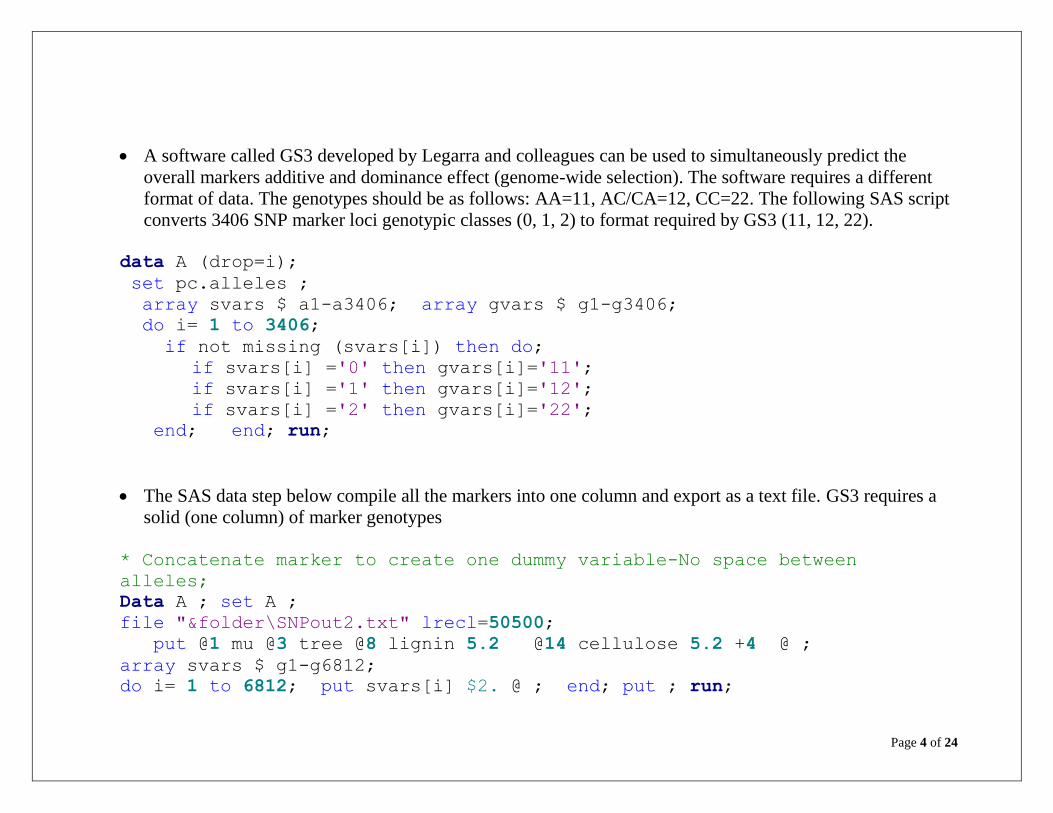
A software called GS3 developed by Legarra and colleagues can be used to simultaneously predict the
overall markers additive and dominance effect (genome-wide selection). The software requires a different
format of data. The genotypes should be as follows: AA=11, AC/CA=12, CC=22. The following SAS script
converts 3406 SNP marker loci genotypic classes (0, 1, 2) to format required by GS3 (11, 12, 22).
data A (drop=i);
set pc.alleles ;
array svars $ a1-a3406; array gvars $ g1-g3406;
do i= 1 to 3406;
if not missing (svars[i]) then do;
if svars[i] ='0' then gvars[i]='11';
if svars[i] ='1' then gvars[i]='12';
if svars[i] ='2' then gvars[i]='22';
end; end; run;
The SAS data step below compile all the markers into one column and export as a text file. GS3 requires a
solid (one column) of marker genotypes
* Concatenate marker to create one dummy variable-No space between
alleles;
Data A ; set A ;
file "&folder\SNPout2.txt" lrecl=50500;
put @1 mu @3 tree @8 lignin 5.2 @14 cellulose 5.2 +4 @ ;
array svars $ g1-g6812;
do i= 1 to 6812; put svars[i] $2. @ ; end; put ; run;

Page 5 of 24
The OUTPUT data (text) is ready to analyze with GS3 and obtain the overall additive, dominance and total
genetic effects of markers (predictions or breeding values of trees)
mu tree trait1 trait2 SNP markers (3406 of them, no space)
1 1 26.57 41.53 121212121212121212121212121212121212
1 2 27.21 41.28 121212121212121212121212121212121212
1 3 27.45 40.30 121212121212121212121212121212121212
mu is a dummy variable needed to fit intercept in genome-wide selection models.
SAS Genetics for Exploratory Marker Data Analysis
The ALLELE procedure in SAS Genetics performs preliminary analyses on genetic marker data:
1. The frequency of homozygous and heterozygous markers,
2. Polymorphic info content (PIC)
3. If a marker is heterozygous, the minor allele frequency for each marker
4. Detect errors in genotyping
5. Test Hardy Weinberg Equilibrium for each marker
Such measures can be useful in determining which markers to use for further linkage or association testing
with a trait. High values of heterozygosity or PIC statistics are a sign of marker informativeness, which is a
desirable property in linkage and association tests.

Page 6 of 24
Proc Allele requires data in different formats to produce above statistics. For example, the procedure
requires that the first two columns in the data contain the set of alleles at the first marker, the second two
columns contain set of alleles at the second marker etc.
Alternatively the columns can be genotypes or one column per each marker. The following DATA step
could be used to produce the desired format for 2963 alleles to summarize data using Proc ALLELE:
data Genotype (drop = i); set A;
array fixit {*} $ snp1 – snp2963; do i = 1 to dim(fixit); fixit(i) = catx("/",substr(fixit(i),1,1),substr(fixit(i),2,1));
end; run;
Output
tree snp1 snp2 snp3 snp4 snp5 snp6 ...
18 A/A A/A A/C A/A A/C A/A
19 A/C A/A A/A A/A A/C A/A
20 A/C A/A A/C A/A A/C A/A
21 A/C A/A A/C A/A C/C A/A
...
The following Proc ALLELE code computes descriptive statistics for 2963 markers using above data format.
The code uses bootstrapping to come up with test statistics
/*computing allele and genotype frequencies*/
proc allele data=genotype outstat=ld prefix=SNP
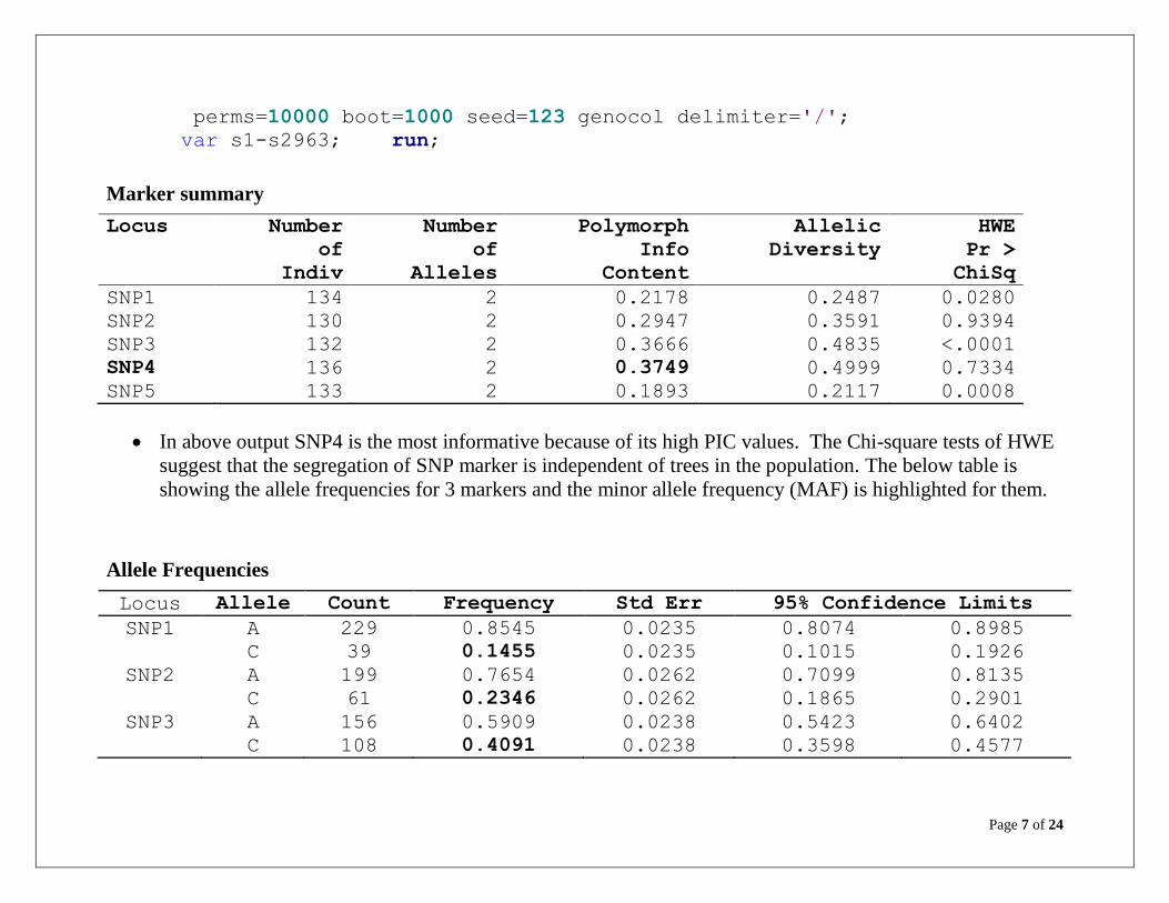
Page 7 of 24
perms=10000 boot=1000 seed=123 genocol delimiter='/';
var s1-s2963; run;
Marker summary
Locus Number
of
Indiv
Number
of
Alleles
Polymorph
Info
Content
Allelic
Diversity
HWE
Pr >
ChiSq
SNP1 134 2 0.2178 0.2487 0.0280
SNP2 130 2 0.2947 0.3591 0.9394
SNP3 132 2 0.3666 0.4835 <.0001
SNP4 136 2 0.3749 0.4999 0.7334
SNP5 133 2 0.1893 0.2117 0.0008
In above output SNP4 is the most informative because of its high PIC values. The Chi-square tests of HWE
suggest that the segregation of SNP marker is independent of trees in the population. The below table is
showing the allele frequencies for 3 markers and the minor allele frequency (MAF) is highlighted for them.
Allele Frequencies
Locus Allele Count Frequency Std Err 95% Confidence Limits
SNP1 A 229 0.8545 0.0235 0.8074 0.8985
C 39 0.1455 0.0235 0.1015 0.1926
SNP2 A 199 0.7654 0.0262 0.7099 0.8135
C 61 0.2346 0.0262 0.1865 0.2901
SNP3 A 156 0.5909 0.0238 0.5423 0.6402
C 108 0.4091 0.0238 0.3598 0.4577

Page 8 of 24
Marker-trait Associations using linear models
SAS/MIXED procedure
For a random mating population with no population structure we can use LS regression to test the association
between a marker and a trait.
y = 1n + Xg + e where mu is the only fixed effect
y = X + e to include other fixed effects
y is a vector of phenotypes, 1n is a vector of 1s, X is a design matrix, g is the fixed effect of the marker and e is a
vector of random errors ~ NID (0, σ2
e).
The null hypothesis (H0) is that the marker has no effect on the trait, while the alternative hypothesis (H1) is that
the marker does affect the trait (because it is in LD with a QTL).
We can use SAS, TASSEL, ASReml or some other software to test the association of each marker with the
phenotype. Based on F-tests we can choose a subset of markers and use them in mixed models to predict breeding
values of trees.
We can create arrays in the data step of SAS to run repeated jobs. The following script creates array for 2963 SNP
markers.
/* Create array for SNPS */
data ds;
set &ds;
array SNP{2963} SNP1-SNP2963;
run;

Page 9 of 24
The MIXED procedure can run mixed models to account for fixed and random effects while testing the null
hypothesis (H0: No association between the marker and trait). The following macro code fits a mixed model to
2963 SNP markers.
%macro genoanova;
%do i=1 %to 2963;
title "SNP &i";
proc mixed data=ds noinfo;
class SNP&i female;
model phenotype = SNP&i ;
random female /solution ;
run;
%end;
%mend;
%genoanova
In above code we get the F-tests for all the markers but also the solutions (best linear unbiased predicted GCA
values) of female. The SOLUTIONS option in the code provides the solutions of mixed model equations (BLUP)
for female effects.
Type 3 Tests of Fixed Effects
Num Den
Effect DF DF F Value Pr > F
SNP1 2 2791 2.07 0.1266
Some remarks about using SAS/Mixed procedure
Marker is fit as fixed effect but can be as random

Page 10 of 24
Additive genetic effects can be modeled and solutions (BLUP) can be obtained.
Not efficient to use pedigrees and marker-based relationship matrices
Not efficient to account for structured populations
Multiple testing problem, sorting out P values and correction for multiple testing
ASReml
ASReml is commonly used in classical BLUP analysis for predictions of breeding values and for estimation of
variance components. It is very powerful software. It allows fitting complicated G and R matrix structures in mixed
models.
A code to test the association of marker and phenotype
Title: clones
clone !P p1 !I p2 !I
famid !A
LOC !A 3 REP *
HT_08 DIA_08 FORK VOL
CF_Pedigree.txt !SKIP 1
CF_clones.csv !SKIP 1 !CSV !EXTRA 5 !NODISPLAY !DOPART 4 !MVINCLUDE
!CYCLE 1:1000
!MBF mbf(clone,1) CFmarker1.csv !SKIP 1 !RFIELD $I !RENAME SNP$I !DDF 2
!FCON # marker data
!PART 1
# This part allows heterogeneous R structure and homogenous G structure ! Heterogeneous errors. SNPs are random

Page 11 of 24
HT_08 ~ mu LOC mv !r SNP$I clone 4.5 !GP ide(clone) 0.5 !GU REP.LOC
1.4 !GU
3 1
780 0 IDEN !S2=11.4842
898 0 IDEN !S2=13.9482
393 0 IDEN !S2=14.1377
# This part allows heterogeneous R structure and correlation structure in G part !PART 4
!CONTINUE
! Multivariate model
HT_08 VOL ~ Trait Tr.LOC Tr.SNP$I !r Trait.clone Trait.ide(clone) Trait.REP.LOC
3 2 3
780 0 IDEN # Site1
Trait 0 US 11.5 0 3.17 !GU
898 0 IDEN # Site2
Trait 0 US 14.1 0 2.79 !GU
393 0 IDEN # Site3
Trait 0 US 11.0 0 2.79 !GU
Trait.clone 2
Trait 0 CORGH !+6 !GU #or !GU
6*0.1
clone 0 AINV
Trait.ide(clone) 2
Trait 0 IDEN 0.2 0.1 0.3
ide(clone) 0 IDEN
Trait.REP.LOC 2
Trait 0 IDEN 0.2 0.1 0.3
REP.LOC 0 IDEN

Page 12 of 24
Some remarks about using ASReml for association testing: Multiple fixed and random effects (max 500 factors)
Additive genetic effects can be modeled and solutions (BLUP) can be obtained.
Efficient to use A matrix, fit multivariate models, heterogeneous R and G structures
Multiple testing problem, sorting out P values and correction for multiple testing
Can utilize user-supplied kinship matrices
TASSEL
The above mixed model can be run with TASSEL to test the
association of markers and phenotype. The software was
developed in Buckler lab and being updated regularly. My
students find TASSEL as a better software to run simpler
mixed models.
Java based, GUI, CLI, does not require expertise and
programming on the part of the user
Handles data and visualizes, A and Q matrices can be
used. Fast and FREE!
Can account for structured populations
Built GLM and MLM for different approaches when
associations are explored
Not designed for multiple design factors, does not fit
markers simultaneously.

Page 13 of 24
What is Allelic Substitution Effect?
Average effect of allelic substitution () represents the average change in phenotype value when A1 allele is
randomly substituted for A2 allele.
= a (1+k (p1-p2))
Where a and k are the gene effects, p1 and p2 are the frequencies of A1 and A2 alleles, respectively. For purely
additive case (k=0), = a (Lynch and Walsh, page 68-69 for more details).
Let assume we have SNPs in the data coded 0, 1, 2. The codes correspond with three genotypes of a single SNP:
0=homozygous (AA), 1=heterozygous (AC), 2=homozygous (CC).
The additive effect can be estimated as the difference between two homozygous means divided by two (Falconer
and Mackay 1996).
A = (AA - CC) / 2
In ASReml, if you leave SNP as a variable and fit it as a fixed effect, you will just have the additive (substitution)
effect. i.e.
y ~ mu SNP !r tree
If you add the term at(SNP,1) as
y ~ mu SNP at(SNP,1) !r tree

Page 14 of 24
then the at(SNP,1) effect will reflect the dominance (D), being the deviation of the SNP=1 class
from the average of the SNP=0 and SNP=2 classes.
D = (AA + CC)/2 - AC
The design matrix for the fixed effects will be
mu SNP at(SNP,1)
1 0 0
1 1 1
1 2 0
and let us say the 3 fitted effects are c (for mu), a for SNP and d for at(SNP,1) So the
SNP=0 class BLUE is c = (mu)
SNP=1 class, BLUE is c + a + d = mu + SNP + at(SNP,1)
SNP=2 class, BLUE is c+2a
at(SNP,1) 1 0.000 0.000
SNP 1 1.316 0.1487
SNP 2 2.534 0.2428
mu 1 2.337 0.1214
Additive effect is (c+2a -c)/2 = a = (2.534-2.337)/2
a is the additive effect and the average allele substitution effect
(Note: The above ASReml solution example was taken from the author of ASReml, A. Gilmour).

Page 15 of 24
Multiple Testing Problem and Q-values
If we choose =0.05 as the significance cut-off point, we will declare 5% of the SNPs significant just by chance
when in fact they are not. In a genome wide association study, we will be testing 10s or possibly 100s of thousands
of markers. If we are testing 100,000 SNPs, we will declare 5000 SNPs significant (false positive) by chance.
Obviously this is a big problem.
There are different ways to control False Discovery Rate
q value (controls the expected proportion of false positives)
Bonferroni test: 1 − (1 − α)1/n
(corrected for n comparisons),
Permutation test (Churchill and Doerge 1994)
Because of space and time limitation, I will not cover details of above approaches but readers should be able to
find details somewhere else easily. For example, there is an easy-to-use R package to calculate Q values from P
values.
R QValue Package
http://cran.r-project.org/web/packages/qvalue/index.html
This package takes a list of p-values resulting from the simultaneous testing of many hypotheses and
estimates their q-values.
The q-value of a test measures the proportion of false positives incurred (called the false discovery rate)
when that particular test is called significant.
Various plots are automatically generated, allowing one to make sensible significance cut-offs. Several
mathematical results have recently been shown on the conservative accuracy of the estimated q-values from
this software.
SAS Macro scripts are available to calculate Q values from P values. They are somewhat cumbersome.
http://www2.sas.com/proceedings/sugi31/190-31.pdf

Page 16 of 24
Statistical Analysis for Genome Wide Selection (GWS)
Two-tier approach: Estimate the SNPs effect first and use the predictions of SNPs to predict Genomic Estimated
Breeding Values of subjects.
Linear model- Each marker is assigned a linear effect in the genome
A traditional BLUP approach - Markers are incorporated assuming equal variance
∑ E(g) is
.
Bayesian approach – uses the prior distribution of QTL effects and allows markers to shrink towards zero (zero
variance explained by some markers).
Very appealing to process large number of markers
Uses different shrinkage factors depending on the informative level of loci
The A matrix is replaced with a genomic relationship matrix (G)
to allow better capturing of Mendelian sampling in the BLUP approach and reduce the selection bias in
Bayesian approaches.
Extension of 1-SNP model by fitting a polygenic effect
y = 1n + Xg + Zu + e where u is the vector of polygenic effect u ~ NID(0, Aσ2
a)
Henderson’s mixed model equations (Hayes 2008).

Page 17 of 24
u
g
ˆ
ˆ̂
yZ'
yX'
y1'
λAZZ'XZ'Z'1
ZX'XX'X'1
Z1'X1'1'11
1
where = σ2
e/ σ2
a = (1-h2) / h
2
Fitting SNPs fixed versus Random effect
Least squares (fixed effect) estimates of SNP effects are equal to the true value + estimation error:
ĝ = g + eĝ
• Thus, SNPs that are significant tend to have larger estimation errors – e.g. SNPs with small minor allele freq.
• This can be addressed by fitting SNP effects as random e.g. assuming g ~ N(0, σ2
g) for some choice of σ2
g.
Fitting g as random regresses or shrinks estimates back to 0 to account for the lack of information. If the choice of
σ2
g is correct (?) then the resulting estimates are BLUP, which have property: g = ĝ + peĝ where peg is the
prediction error.
Note the similarity to BLUP estimation of breeding values.
Differences between random / fixed are small if the amount of data is large (small errors) or if λg= σ2
e/σ2
g.
Add λg to the diagonal of the X’X matrix.
2 is small
u
g
ˆ
ˆ̂
yZ'
yX'
y1'
λAZZ'XZ'Z'1
ZX'IλXX'X'1
Z1'X1'1'11
1
g
σ2
g could be set such that Xig explains variance equal to some value = σ2M

Page 18 of 24
SNP: A biallelic locus with two alleles (1 and 2). The allele ‘2’ has a positive effect on phenotype.
y = 1n + Xg + Zu + e where u is the vector of polygenic effect u ~ NID(0, Aσ2
a)
Using the solutions from the mixed models we can set up another linear model ̂ ̂ to calculate
Marker-Assisted BVs of progeny with no phenotypic records.
Effect Estimate
Mu 2.96
G 0.87
U
1 0.56
2 -0.01
... ...
10 0.09
11 0.28
12 0.43
13 -0.67
14 -0.56
15 -0.48
GS3 for Genomic Selection – GIBBS Sampling – Gauss Siedel (By A. Legarra)
A unified single step approach, simpler than two-tier approach
Utilize genomic and phenotypic information into a single set of equations
Reduce the bias from association testing
Animal g-hat X u-hat Xg+u-hat MEBV
11 0.87 1 0.28 =0.87*X+u 1.15
12
1 0.43 1.30
13
0 -0.67 -0.67
14
1 -0.56 0.31
15
2 -0.48 1.26

Page 19 of 24
Uses GIBBS sampling to estimate standard errors of effects
All the markers are fit simultaneously
∑
Where y is the i-th phenotype, Zijk is indicator variable for the i-th individual, j-th marker locus and k-th allelic
form, and e is residual error term. aj is half the difference between the two homozygotes
The additive effects (allelic substitution effect) of the SNP's when ajk =11 or 22,
When the genotype is 12, then the solution is dominant effect
Fits any number of random effects, additive a, dominance marker effects d, polygenic effects u and
permanent environmental effects c.
y = Xb + Za +Wd+ Tu + Sc + e
Require a parameter file (shown below)
DATAFILE
SNPout.txt
PEDIGREE FILE
PCPedigree.txt
NUMBER OF LOCI (might be 0)
3406
METHOD (BLUP/MCMCBLUP/VCE/PREDICT)
BLUP
GIBBS SAMPLING PARAMETERS
NITER

Page 20 of 24
10000
BURNIN
2000
THIN
10
CONV_CRIT (MEANINGFUL IF BLUP)
1d-4
CORRECTION (to avoid numerical problems)
1000
VARIANCE COMPONENTS SAMPLES
var.tree.txt
SOLUTION FILE
solutions.tree.txt
TRAIT AND WEIGHT COLUMNS
3 0
NUMBER OF EFFECTS
4
POSITION IN DATA FILE TYPE OF EFFECT NUMBER OF LEVELS
1 cross 1
2 add_animal 150
5 add_SNP 3406
5 dom_SNP 3406
FORMAT
(f1.0,f2.0,f9.0,f6.0,4x,a6812)
VARIANCE COMPONENTS (fixed for any BLUP, starting values for VCE)
vara
2.52d-04 -2
vard
1.75d-06 -2
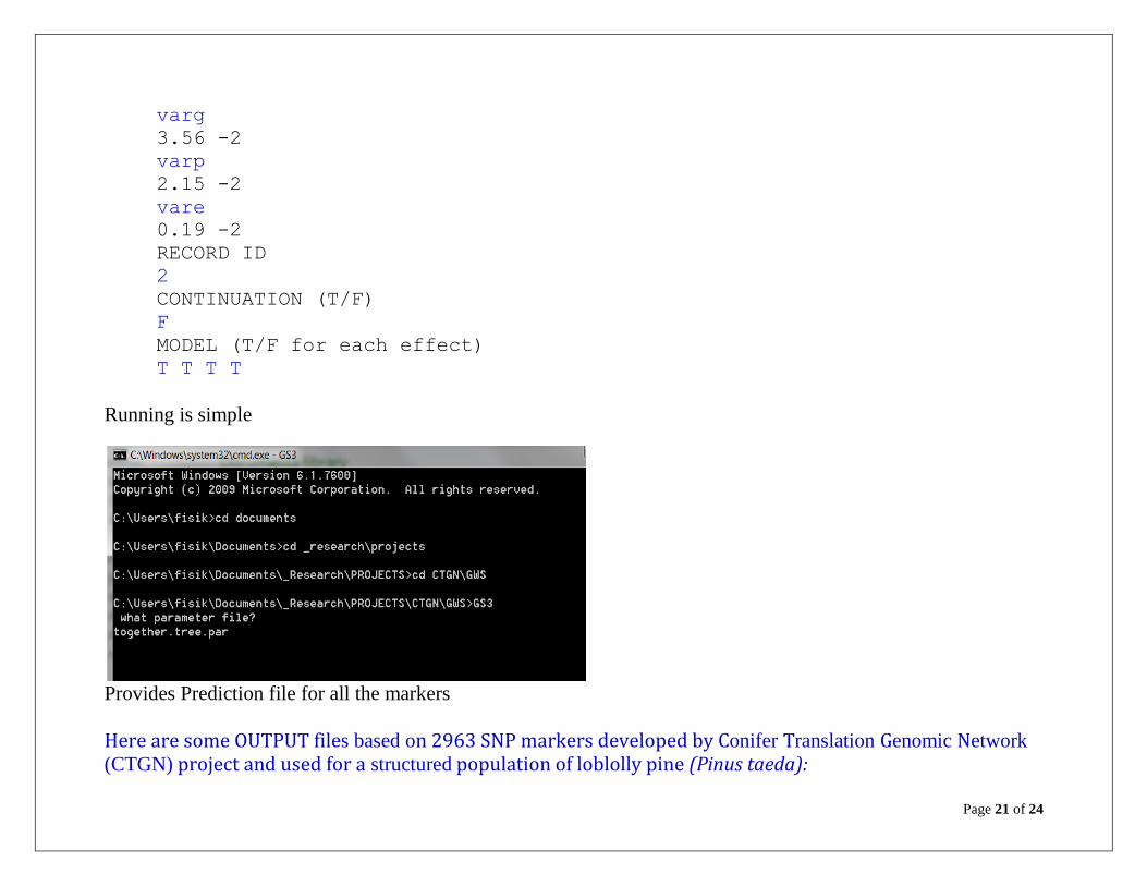
Page 21 of 24
varg
3.56 -2
varp
2.15 -2
vare
0.19 -2
RECORD ID
2
CONTINUATION (T/F)
F
MODEL (T/F for each effect)
T T T T
Running is simple
Provides Prediction file for all the markers
Here are some OUTPUT files based on 2963 SNP markers developed by Conifer Translation Genomic Network
(CTGN) project and used for a structured population of loblolly pine (Pinus taeda):

Page 22 of 24
EBVs – Predicted BVs of trees
id EBV_aSNP EBV_dSNP EBV_anim EBV_overall
1 -709.905 -3.79700 995.929 282.226
2 -261.545 -3.49217 -567.143 -832.181
3 -178.986 -1.52097 -711.054 -891.561
4 -51.7698 -3.07897 -806.308 -861.157
5 69.3529 -1.99274 -715.816 -648.456
EBV_aSNP = Sum of marker loci additive effect
EBV_dSNP = Sum of marker loci dominant effect
EBV_anim = Polygenic breeding value
EBV_overall = Sum of polygenic, marker additive and dominance breeding value
SOLUTIONS
effect level solution sderror
1 1 1063.0348 0.0000000 (overall mean)
2 1 995.92865 0.0000000
2 2 -567.14322 0.0000000
2 3 -711.05403 0.0000000
2 4 -806.30775 0.0000000
3 1 2.2089452 0.0000000 (BLUP pred. for SNP 1)
3 2 0.90101161 0.0000000 (BLUP pred. for SNP 2)
3 3 -2.6428882 0.0000000

Page 23 of 24
Cross validation
Split data into y1 and y2 (validation) and predict observations in y2 using parameters from y1.
(y2|y1). Use person correlation r(ŷ2 | y2) to measure the success (predictive ability).
Prediction
The program computes predicted phenotypes given the model parameters. It generates overall genetic values if a, d
and u are given. If we have trees with no phenotypes and we want to get predictions using markers and model
parameters, we can choose PREDICT option. For complete data, the PREDICT estimates the correlation (r(ŷ2 |
y2)) of observed phenotype (y1) and predicted phenotype (ŷ2). For 150 pine clones the correlation for lignin
content was 0.88.
Training and validation sets
1/5 to 1/10 of data for validation if data are small. For 1000 animals split the data.

Page 24 of 24
Literature:
Kang HM, Zaitlen NA, Wade CM, et al. (2008) Efficient control of population structure in model organism association mapping.
Genetics 178:1709–23.
Legarra A, Misztal I. Technical note: computing strategies in genome-wide selection. JDairy Sci 2008;91:360–6.
Legarra et al. 2008. Genetics.
Zhiwu Zhang, Edward S. Buckler, Terry M. Casstevens and Peter J. Bradbury (2009) Software engineering the mixed model for
genome-wide association studies on large samples, Briefing in Bioinformatics, 6:664-675.