Please cite this paper as:

Vavra, P. and B. K. Goodwin (2005), "Analysis of PriceTransmission Along the Food Chain", OECD Food,Agriculture and Fisheries Working Papers, No. 3, OECDPublishing.doi:10.1787/752335872456

OECD Food, Agriculture and FisheriesWorking Papers No. 3

Analysis of PriceTransmission Along theFood Chain

Pavel Vavra*, Barry K. Goodwin

JEL Classification: C22, D4, Q13

*OECD, France

2

TABLE OF CONTENTS

Introduction ................................................................................................................................... 3

Price Transmission in Agricultural Markets.................................................................................. 4

Price Transmission Estimation Methods ..................................................................................... 11

Asymmetric Price Transmission ������������������� ��� ..................................................... 15

Conclusions ................................................................................................................................. 19

References ................................................................................................................................... 21

Glossary of Terms ....................................................................................................................... 27

Annex 1. Time Series Analysis – Brief Overview ...................................................................... 29

Annex 2. Threshold Vector Error Correction Model................................................................... 35

Annex 3. The Estimation Procedure............................................................................................ 39

Annex 4. US Farm, Wholesale and Retail Monthly Prices for Beef, Chicken and Eggs ............ 41

Annex 5. Results of the Empirical Application........................................................................... 42

The authors of this paper are Pavel Vavra, OECD Directorate for Food, Agriculture and Fisheries, and Barry K. Goodwin of North Carolina State University. The views expressed in this paper are those of the authors and do not necessarily represent those of the OECD or its Member governments. The authors would like to acknowledge the helpful comments received by Wyatt Thompson and Frank Bunte.

3

ANALYSIS OF PRICE TRANSMISSION ALONG THE FOOD CHAIN

Introduction

The interest in marketing margins and price transmission has recently gained remarkable momentum and the amount of studies on this subject is rapidly growing. There is a myriad of questions about prices and margins investigated by these studies, yet new questions are surfacing as markets and business practices change with an impressive speed. Wohlgenant (2001), in his survey on marketing margins, identifies some of the questions puzzling researchers and policy makers alike. For example: Are marketing margins too large? Why are margins different among products? How have margins changed over time? What is the incidence of marketing costs on retail prices and farm prices? How quickly are farm prices transmitted to the retail level and vice versa? What is the relationship between concentration and market power? Is increased concentration detrimental or beneficial to producers?

With quickly changing market structures, growing concentration of processing and retail firms, these types of questions are attracting greater public scrutiny. The topic of “Economic Impacts of Increasing Market Concentration on Consumers, Processors and Farmers” is the focus of activity H of the Committee for Agriculture’s Programme of Work for 2005 and 2006. This report focuses on one particular aspect of the broader subject – the assessment of price transmission along the supply chain. In other words, the report addresses the question: “How quickly and to what extent are changes in farm prices transmitted to the retail level and vice versa?”

It is important here to distinguish between analyses of evolution of margins over time and price transmission as these topics are closely related but are not identical. Conclusions about price transmission that are drawn from the evolution of marketing margins over time, but that do not incorporate other information such as the changes in the costs of other inputs, may well be misleading.1 This paper limits itself to an analysis of vertical price transmission.

The adjustment to price shocks along the chain from producer to wholesale and to retail levels, and vice versa, is an important characteristic of the functioning of markets. As such, the process of price transmission through the supply chain has long attracted the attention of agricultural economists, as well as policy makers. Recently, the subject of price transmission has been increasingly linked to the discussion about benefits from agricultural reform. That is, a common concern of policy makers relates to the assertion that, due to imperfect price transmission (perceived to be caused by market power and oligopolistic behaviour), a price reduction at the farm level is only slowly, and possibly not fully, transmitted through the supply chain. In contrast, price increases at the farm level are thought to be passed more quickly on to the final consumer.

An implication of this asymmetry in price transmission, if it exists, is that an analysis of trade liberalisation likely over-estimates the benefits to consumers in countries that have gone through

1. For example, costs related to processing, packaging, moving, advertising and storing.

4

policy reform, because the reduction in farm prices might not be immediately or fully transmitted to final consumers.2 As a result, there would be smaller positive effects on consumer welfare and a possible increase in rents for the firms in the downstream sector. Thus, it is important to understand the processes related to pass-though of price changes as price transmission assumptions along the supply chain play an important role in determining the size and distribution of welfare effects of trade policy reform.

It should be noted that market power might be an important explanation for any evidence of asymmetries in price transmission, but it may not be the only causal factor. That is, incomplete or asymmetric price transmission may take place for a number of other reasons. In fact, Peltzman (2002) argues that asymmetric price transmission may be characteristic of competitive, as well as oligopolistic market structures, and it cannot simply be concluded that presence of asymmetric price transmission automatically implies market power.

The aim of this paper is to review the mechanisms of asymmetric price transmission and to explore tests that measure asymmetric price transmission empirically. The paper starts by identifying possible asymmetric response of prices and reviews the main reasons put forward in the various studies that explain imperfect price transmission and asymmetries. The discussion of empirical findings will limit itself, to a large extent, to research of asymmetric price transmission for agricultural commodities. This discussion will be followed by a review of methods employed to estimate price transmission. The method proposed for the testing of asymmetric price transmission will be described and illustrated empirically for a small set of commodities. At this stage, the present study does not attempt to draw any conclusions or implications for policy.

Price transmission in agricultural markets

Economists have long been concerned with the transmission of market shocks through the various stages of the supply chain, or through horizontally related markets. Much of this research has examined the role of price as a mechanism for characterising the linkages among market levels.

The literature analysing horizontal price linkages dates back more than one-hundred years and was typically concerned with spatial price relationships, i.e. links between prices at different locations. Concepts pertaining to the spatial transmission of price shocks play, for example, a very important role in theories associated with exchange rate determination and market integration. Much of this literature has been concerned with the “law of one price” or, at an aggregate level, with “purchasing power parity.”3 Although the methods of testing for empirical evidence may have indirect relevance to the objectives of the present study, this body of research is not directly applicable.

The literature analysing vertical price linkages has concentrated on evaluations of the links between farm, wholesale and retail prices. The vertical price relationships have featured prominently in recent studies as commodity markets have become more highly concentrated at each level and integrated across levels. Vertical price transmission is the focus of this study also, and the literature review below summarises briefly work in this field. 2. The evaluation of trade liberalisation welfare impacts need to take into account not only the vertical

but also the horizontal price transmission; in other words, the level of market integration.

3. Examples of studies in the context of the Law of One Price, purchasing power parity and market integration include Dornbush (1987), Ardeni (1989), Baffes (1991), Gardner and Brooks (1994), Blauch (1997), Tkacz (2001), Baffes and Ajwad (2001), Goodwin and Piggot (2001), Jamaleh (2002), Barret (2001), Seo (2003), Brooks and Melyukina (2003), FAO (2003), Balcombe (2003), and Brooks and Melyukina (2004).

5

Aspects of vertical price transmission

Vertical price relationships are typically characterised by the magnitude, speed and nature of the adjustments through the supply chain to market shocks that are generated at different levels of the marketing process. In the context of this definition, the underlying links across agents at different levels of activity, from production to consumption and vice versa, may be summarised in a single set of measures that define the speed and size of the impacts of a shock in prices at one level on the prices up- or downstream. For example, if a positive shock in the primary commodity market at the farm level induces an upward shock to the farm price, then what is the size and timing of any impacts on wholesale and retail prices? Alternatively, one can evaluate the impacts on farm level prices following a shock whose first incidence is on retail prices.

The size of effects that are transmitted across levels is typically of central concern, although the speed of adjustment is equally important. The speed with which markets adjust to shocks is determined by the actions of market agents who are involved in the transactions that link market levels; i.e. wholesalers, distributors, processors, retailing firms and the like. If adjustment is costly or is otherwise subject to constraints, price signals passed from agent to agent may take place only with delays where lags may be significant. That is, increases or decreases in one end of the chain are not transmitted instantaneously but instead distributed over time. In the extreme case of very high transaction costs, even highly competitive firms may fail to adjust to small price changes and, consequently, prohibit the transmission of some shocks across market levels. In this context, the size of shocks may be important to the extent of any reaction by other markets.

Recent research has recognized more complex aspects of price transmission relationships and explored the extent to which price adjustments may be asymmetric. These studies typically distinguish between positive and negative price shocks. A finding of asymmetric price transmission may allow a researcher to make some inferences about the behaviour of agents in the market, particularly as their actions impact on links across different market levels. Peltzman (2000) argues that asymmetric price transmission is the rule, rather than the exception, and concludes that, since asymmetric price transmission is prevalent in the majority of producer and consumer markets, standard economic theory that does not account for this situation must be incorrect.

The issue of asymmetric price transmission is taking on renewed prominence due to its potentially important welfare and policy implications. Meyer and von Cramon-Taubadel (2004) observe that a possible implication of asymmetric price transmission is that consumers are not benefiting from a price reduction at the producers’ level, or producers might not benefit from a price increase at the retail level. Thus, under asymmetric price transmission, the distribution of welfare effects across levels and among agents following shocks to a market will be altered relative to the case of symmetric price transmission.4

In general, the primary focus of studies that analyse vertical price transmission is the assessment of the characteristics noted above: the extent of adjustment, the timing of the adjustment and the extent to which adjustments are asymmetric. These aspects can be restated as four fundamental questions:

� How big is the response at each level due to a shock of a given size at another level? (magnitude)

� Are there significant lags in adjustment? (speed) 4. In making welfare evaluations, it is important to take the transaction costs of changing prices into

account. The issue of transaction costs, such as adjustment and menu costs, is discussed later in this paper.

6

� Do adjustments following positive and negative shocks at a certain marketing level exhibit asymmetry? (nature)

� Do adjustments differ depending on whether a shock is transmitted upwards or downwards the supply chain? (direction)

It should be noted that asymmetries can occur within any aspect of the adjustment process. Price transmission might be asymmetric in its speed and magnitude, and could differ depending on whether the price shock is positive or negative and is being transmitted upwards or downwards along the chain. Figure 1 shows shock adjustment down the marketing chain. The figure illustrates a positive and a negative shock of the same magnitude in one period, t1, to an input price, Pi, and the adjustment in output price, Pj . Thus, in this example, the initial incidence of the shock is on the producer price of the commodity, and the impulse is transmitted, according to some underlying process, to the retail price. In the figure ��i

+ and ��i� are positive and negative shocks of the same magnitude to the producer

price, ��jm is the adjustment in the retail price to the positive producer price shock, ��jn is the adjustment in the retail price to the negative producer price shock, ��j k is the time lag for adjustment in the retail price to the positive producer price shock, while ��j l is the time lag for adjustment in the retail price to the negative producer price shock.

The figure illustrates how the positive shock on the producer price, ��i, in the first period, t1, triggers a response in the retail price, ��jm, over a period of time, ��j k. It is important to note that the absolute and relative change in producer price in the hypothetical example shown here is more than the change in retail price, ��i

+ > ��jm.. Thus, in this case, the initial price increase at one level has not

been fully transmitted up the supply chain even after several periods. Similarly, the figure shows that in the case of a negative shock, the decrease in producer price, ��i

�, does not lead to an equivalent change in retail price in this illustrative example. Note that in this illustrative case the magnitude and speed of price transmission differ depending on the nature of the shock, ��jm>��jn. and ��j k > ��j l .

Figure 1. Illustration of an asymmetric vertical price transmission (two levels)

PRICE

TIME t2 t3 t1

� Pj m

� Pi+

� Pi�

t4

�P j n

�t j l

�t j k

Pj

Pi

Overall, in this hypothetical example, four basic outcomes can be observed and the final impacts at the extreme end of the marketing chain may differ in timing and magnitude relative to the initial

7

shock, and may also vary depending on the nature of the initial shock.5 The shock origin at the input (farm) level in the above example is consistent with the presumption that the direction of causality runs from the farm to retail levels. In fact, the majority of studies have analysed price transmission from the farm to the retail level, not vice versa. However, to understand the functioning of the markets, it seems to be equally important to analyse the extent of transmission of a shock in output (retail) prices up the supply chain.6 Different adjustments in input price, Pi, to positive and negative shocks in output price, Pj, could be easily illustrated by inverting the diagram in Figure 1.

The adjustment to a price shock could be also elaborated further by adding another price level into the diagram, such as a wholesale price, to show the successive pass-through of a price shock that originates on either end of the marketing chain. Obviously, the presence of imperfect price transmission among the intermediate stages would inhibit price transmission from one extreme end of a marketing chain to the other. Peltzman (2000) found above average asymmetry between producer and consumer prices when there were many small intermediaries present in between the producer and retail level. McCorriston and Sheldon (1996) have shown that the higher the number of stages in the vertical market structure that are characterised by market power of the actors in these stages, the likelier is a lower pass-through of price changes.7 In addition, the shock may not necessarily originate only at the ends of the supply chain. Bunte and Kuiper (2003) argue that for a small, open economy, a shock may in fact originate at the wholesale level where international price levels are being determined.

Causes of asymmetric price transmission and empirical findings

A number of reasons are put forward in the literature that attempt to explain the asymmetries and imperfect pass-through of prices.8 Many of these arguments relate to an adjustment problem at the retail level and so-called “sticky” prices. For example, prices at the retail level may not adjust due to menu costs, which are costs associated with making changes in retail prices such as advertising and labelling, as well as the risk to the retailer’s reputation if its price changes are frequent. Uncertainty of whether the price shock is permanent or transitory exacerbates a firm’s reluctance to respond to price signals.

Ball and Mankiw (1994) note that in the presence of inflation and nominal input price shocks the use of menu costs by agents may lead to more resistance to lower prices than to increase them. Bailey and Brorsen (1989) also pointed out that asymmetries in price adjustments may be caused by asymmetries in the underlying costs of adjustments. Alternatively, retailers selling perishable goods might be reluctant to raise prices in line with an increase in farm-level prices given the risk that they

5. Note that if a fall in farm prices is not followed imediately downstream while a rise in farm prices is,

these changes are detrimental for farmers and consumers but beneficial for other parties further downstream, notably processors and retailers. On the contrary, if a fall in farm prices is followed immediately downstream while a rise in farm prices is not, these asymmetries would be beneficial for farmers and consumers but detrimental for processors and retailers.

6. As an example, Tiffin and Dawson (2000) show that a long-run relationship exists between producer and retail prices of lamb in the UK, with causality running from retail to producer price. On the other hand, price changes at the producer level result in short-run disequilibria, according to their findings, and have no long-run impact on retail prices.

7. The broad theoretical framework for measuring impacts of successive monopolies in a vertical market chain was illustrated in Cotterill (2002).

8. A comprehensive review of the causes of asymmetric price transmission is provided by Meyer and von Cramon-Taubadel (2004).

8

will be left with unsold spoiled product (Ward, 1982). Note that this would cause asymmetries in price changes that are beneficial for suppliers and consumers and detrimental for retailers. However, Heien (1980) argued that changing prices is more costly for products with a long shelf life as these costs include loss of goodwill. Blinder (1994) and Blinder et al. (1998) found that merchants often believed themselves to be disciplined by a fear of being “out of line” with their market competitors when costs rose, implying asymmetric responses to cost increases and decreases.

Response might also be asymmetric due to inventory management strategies. Retailers may reduce their prices more slowly compared to reduction in farm-level prices to avoid running out of stock (Reagan and Weitzman, 1982). Balke et al. (1998) show that accounting methods such as FIFO (first in first out) could cause asymmetric adjustments to price shocks. Wohlgenant (1985) also demonstrated that lags between retail and wholesale food prices can be explained by the inventory behaviour of retailers. The argument that stock building and the non-negative constraint on inventory could lead to asymmetric price responses was also put forward by Blinder (1982).

Gardner (1975) pointed out that, in addition to other causes, farm-to-retail price asymmetries might be the result of government intervention to support producer prices. Similarly, Kinnucan and Forker (1987) argued that government policies may lead to asymmetric price adjustments if agents believe that price movements in one direction may be more likely to trigger government intervention than movements in another direction: the government may be more likely to intervene if market shocks lower producer prices than if producer prices increase. The authors estimated price transmission for dairy products in the United States and showed that transmission elasticities for rising farm prices were larger than corresponding elasticities associated with falling farm prices, depending on the dairy product. Serra and Goodwin (2003) studied price transmission in the Spanish dairy sector and argued that scarcity of milk, to some extent created by the quota system, may lead to a situation in which processors compete to increase both their access to milk quota and their retail market share, but may not pass the resulting farm level price increase fully to the retail level.

Although these and other explanations have been discussed and even demonstrated theoretically or empirically, it is the presence of non-competitive behaviour in the market place that is often identified as, or claimed to be, the culprit for asymmetric price transmission. However, the discussion of asymmetric price adjustments has taken place in the shadow of widespread suspicions that agents in concentrated industries are pricing in a manner to capture welfare, and profits, for themselves, rather than behave in a competitive manner and allow price signals to pass up and down the chain unmolested. Likewise, when observers consider interaction between highly concentrated processors and “stereotyped” small farmers, the common belief is that processors may be more likely to pass to these farmers down-stream price decreases than down-stream price increases. In both cases, the asymmetric price transmission results from the concentrated agents’ exploitation of their perceived market power.9 Zachariasse and Bunte (2003) note that market power may explain why prices are not fully transmitted while oligopolistic and oligopsonistic interdependence may give rise to lags in price adjustment. They argue that the risk of invoking a price war may make firms reluctant to lower prices, leading to an asymmetry in the price reaction to positive versus negative price shocks.

Wann and Sexton (1992) modelled the California pear industry and showed retail price enhancement above the competitive norm in canned pear and fruit cocktail markets, although the hypothesis of competition in the raw pear input market was rejected. The asymmetry in price transmission due to market power, albeit at a local level, was also noted by Benson and Faminow (1985) who argued that a consumer’s choice between food stores is based on location convenience and 9. The most common definition of market power in Industrial Organisation theory is the ability to raise

prices above marginal costs.

9

is made in the presence of search costs, thus creating locally imperfect markets. Gohin and Guyomard (2000), using a structural model, strongly rejected the hypothesis that French food retail firms behave competitively and illustrated that more than 20% and 17% of the wholesale-to retail price margins for dairy and meat products, respectively, can be attributed to oligopoly-oligopsony distortions. Abdulai (2002) illustrated that increases in producer prices of pork in Switzerland are passed on to retail prices faster than reductions in producer prices. Similarly, von Cramon-Taubadel (1998) found that wholesale prices in German pork markets reacted more rapidly to positive shocks than to negative shocks originating at the farm level.

Although market power has been identified as the main cause of imperfect price transmission in some cases, and is widely suspected in others, recent research shows that this does not always have to be the case. McCorriston et al. (2001) demonstrated that price changes can be greater or smaller than the competitive benchmark case depending on the interaction between market power and returns to scale. These authors show that, if the cost function is characterised by increasing returns to scale, the influence of market power might be offset by the costs effects of scale enlargement and the level of price transmission may increase relative to the competitive case. Weldegebriel (2004) also argued that the presence of oligopoly and oligopsony power does not necessarily mean imperfect price transmission. The author illustrated that the functional forms of retail demand and farm input supply are key factors in determining the level of price transmission. Azzam (1999), using a two-period model of spatially competitive retailers, has shown that asymmetry can occur even in a competitive environment due to intertemporal optimizing behaviour, so that retail prices may rise relatively more than decline in response to a corresponding direction of shocks in producer prices.

Bettendorf and Verboven (2000), using a model of oligopolistic interaction, showed that the weak transmission of coffee bean prices to consumer prices in the Netherlands was due to a relatively large share of costs other than the costs of beans. The authors concluded that the market was relatively competitive. Empirical results of Holloway (1991) suggest that, during the period 1955-83, departures from competition in the retail markets of the major food groups have been relatively insignificant, in that estimated results are not statistically different from the outcomes under perfect competition. Zachariasse and Bunte (2003) also found limited evidence for the abuse of market power in Dutch food processing and retail trade and argue that adjustment costs are probably a more important explanation of poor price transmission than market power. Serra and Goodwin (2003) demonstrated that asymmetries were not present in the price transmission of highly perishable dairy products in Spain, supporting the theory that market power could be consistent with symmetric price relationships.

London Economics (2003) investigated the links between retail and farm-gate milk prices in the UK, Denmark, France and Germany. The study found that, in the UK, a unit increase in the retail price of liquid milk is fully transmitted to the farm gate price, whereas a unit increase in farm gate prices results in only a 0.56 unit increase in the price at retail and a unit decrease in farm gate price reduces the retail price by 0.71 unit. In Germany, the study also found two-way price transmission, though rather imperfect. In Denmark, no evidence was found of price transmission in any direction at all. In France, farm-gate price changes were mostly, but imperfectly, transmitted to retail prices. The study associated some of the resulting differences among countries to differences in market structures, differences in the transmission of information or varying degrees of government intervention.

The U.K. Department for Environment, Food and Rural Affairs (DEFRA) commissioned a major study investigating the determinants of farm-to-retail price spreads in the UK and several EU countries (London Economics, 2004). The study investigates the evolution of farm and retail prices during the 1990’s for about 90 products. The report finds very little evidence of systematic asymmetric transmission in the EU food chains, with the possible exception of certain dairy products, which

10

showed very low price transmission.10 The study also found no evidence that particular countries have systematically more asymmetric price transmission in the food chain than others, perhaps with the exception of France where farm-gate and retail food prices did not seem to exhibit a stable relationship over the long run. The report also investigates the impact of increased concentration in food retailing on price transmission. A semi-structural model is chosen because it allows capture of the sensitivity of price spreads to various elements, such as costs along the vertical supply chain (from farmers to consumers), demand and supply of the product, EU intervention prices under the Common Agricultural Policy (CAP), relevant exchange rates and competition in the retail market. The model was estimated for four broad categories of products including wheat products, red meat, poultry and fruit and vegetables. The report concludes that the empirical estimation results did not point to a systematic widening of farm-to-retail price spreads as a result of potentially stronger buyer power caused by increasing concentration in the food retail sector.11

Inconclusive evidence from the literature

Despite a large number of studies that have investigated the phenomenon of price transmission in agricultural markets, it is not possible to draw strong conclusions upon which policy decisions could be based. Although many studies seeking imperfect price transmission have found support for it, the evidence is often mixed and varies widely across commodities and countries.12

The one inarguable conclusion to draw from the literature summarised here might be that more research is needed in order to understand the increasingly complicated relationships among prices along the supply chain and the underlying behaviour of agents.13 Similarly, in the introduction to their survey, Meyer and von Cramon-Taubadel (2004) argue that there is still a considerable need for further research, and that it would be premature to draw far-reaching conclusions for theory and policy on the basis of work to date. The authors plead that economists should think carefully about the theories that explain asymmetric price transmission. In addition, they argue that the common tests to measure the transmission need to be reliable and precise in the statistical sense, but also need to be able to distinguish whether evidence of imperfect price transmission is economically relevant.

10. The report notes, however, that the results for dairy products are based on data available only from

1995 to 2001, a time series which might be deemed too short for reliable estimation.

11. Conversely, a large report on dairy supply chain margins by MDC (2004) argues that over the past ten years farm-gate prices and total farm-to-retail margins have fallen, but dairy processor margins have remained fairly constant while retailer margins have increased across all products. However, to re-emphasise an observation stated before, a change in the farmer’s share of the retail margin does not necessarily point to imperfect price transmission and has to be evaluated against the development of other input costs.

12. The literature on asymmetric price transmission is typically not very strong in explaining the imperfections found. On the other hand, structural models are better in finding explanations for imperfections in price transmission, but do not focus on asymmetries of the transmission. Structural models analyse pricing behaviour on the basis of explicitly modelled demand and supply equations.

13. For example, pricing behaviour of large supermarkets is becoming increasingly sophisticated further blurring the price relationships along the food chain. Chevalier et al. (2003) explain rather counter intuitive observation of falling consumer prices during peak demand period using the “loss leader” model of retail behaviour in which the retailer advertises discounted products in an attempt to compete with others. In addition, the use of contracts in agricultural markets is rapidly increasing, with possible impacts on markets and pricing as discussed in USDA (2004).

11

Price transmission estimation methods

As noted above, a large number of studies have examined price transmission in agricultural commodity markets. The choice among various possible techniques applied in each of these studies depended on the questions asked, the data used and the assumptions made. Many empirical studies were concerned with the determinants of retail, wholesale and farm prices, leading authors to use structural models (Gardner, 1975; Cowling and Waterson, 1979). A number of studies also developed techniques to test for the presence and impact of market power with a view to answer concerns about the potential effects that increased market concentration may have on price adjustment processes. A review of the empirical issues underlying this literature can be found in Wohlgenant (2001).

A comprehensive review of estimating and testing for asymmetric price transmission is provided in Meyer and von Cramon-Taubadel (2004). The authors note that there is a long history of asymmetric price studies starting with Tweeten and Quance (1969), who use a dummy variable technique to estimate irreversible supply functions. In their technique, the dummy variables are used to split the input price into two parts: one variable includes only increasing input prices and another includes only decreasing input prices. From this, two input price adjustment coefficients can be estimated. Symmetric price transmission is rejected if these coefficients are significantly different from one another. This technique was later adapted, with many refinements to the study of asymmetric price transmission. Based on Tweeten and Quance, Wolffram (1971) proposes a variable-splitting technique that explicitly includes first differences of prices in the equation to be estimated. Houck (1979) modified this technique further to exclude the initial observations because, when considering observation-to-observation differential effects, the level of the first observation will have no independent explanatory power.

Ward (1982) extends Houck’s specification by including lags of the exogenous variables such that the delay in effects and the length of lags, can differ depending on whether the causal price is increasing or decreasing. Boyd and Brorsen (1988) were the first to use lags to differentiate between the magnitude and the speed of transmission. Based on comparisons of individual estimated coefficients, they analyse the speed of price transmission in specific periods and, based on the sums of these coefficients, they analyse its magnitude. Meyer and von Cramon-Taubadel (2004) called the above techniques the pre-cointegration techniques.14 The typical specifications involved a regression of price differences on lagged price differences, where the lagged differences are segregated according to sign, so that positive changes are allowed to have a different effect than negative changes.

There is an extensive list of studies that have used the above techniques. Examples include studies on asymmetry in farm-to-retail price transmission in the dairy sector (Kinnucan and Forker, 1987), price asymmetry in the U.S. pork markets (Boyd and Brorsen, 1988), asymmetry in spatial fed cattle markets (Bailey and Brorsen, 1989), price transmission asymmetry in pork and beef markets (Hahn, 1990), a study of the Alberta pork market (Punyawadee, et al. 1991), price asymmetry in the international wheat market (Mohanty, et al., 1995), price asymmetry in the peanut butter market (Zhang, et al., 1995), asymmetric price relationships in the U.S. broiler industry (Bernard and Willett, 1996), asymmetries in farm to retail price transmission of fresh tomatoes, onions, powder milk, soluble coffee, rice, and beans in Brazil (Aguiar and Santana, 2002), and price asymmetry of fresh tomatoes in the U.S. (Girapunthong et al, 2003).

Although the above studies have an intuitive appeal, recent research has given more careful consideration to the time-series properties of the price data. Many economic time series are non- 14. Hahn (1990) attempted to generalise these so called pre-cointegration approaches by proposing a

Generalised Switching Model.

12

stationary. In the presence of non-stationary variables, there might be what Granger and Newbold (1974) call a spurious regression result in that there appears to be a significant relationship among variables, but the results are in fact a statistical artefact without any economic meaning. Thus, testing for non-stationarity and the potential for co-integrating relationships among prices at various levels of the market have become an important part of price transmission models. Annex 1 introduces some basic notions about time series and explains the importance of non-stationarity and co-integration.

Von Cramon-Taubadel and Fahlbusch (1994) were among the first to incorporate the concept of cointegration into models of asymmetric price transmission. The authors pointed out the potential for spurious regression results in the case of asymmetry tests based on techniques discussed above, in particular the pre-co-integration techniques. They suggest that, in the case of co-integration between non-stationary time series, an error correction model (ECM), extended by the incorporation of asymmetric adjustment terms, provides a more appropriate specification for testing asymmetric price transmission. This method allows for asymmetric adjustments by distinguishing between positive and negative shocks to error correction terms. The basic concept and definition of an ECM is described in Annex 1, together with a brief explanation of the Von Cramon-Taubadel and Fahlbusch (1994) testing procedure for asymmetric price transmission.

There are a number of studies that have used this approach, or some variant. For example, von Cramon-Taubadel and Loy (1996) use an ECM to study spatial asymmetric price transmission on world wheat markets. Scholnick (1996) also uses an ECM to test for asymmetric adjustment of interest rates, while Borenstein et al. (1997) employ an ECM specification where the error correction terms are not segmented. Von Cramon-Taubadel (1998) estimated price transmission in German pork markets using ECM. Balke et al. (1998) and Frost and Bowden (1999) also employ variants of the asymmetric ECM. FAO (2003) provides a review of the application of time series techniques (co-integration, ECMs) in testing market integration and price transmission for a number of cash and food crop markets in developing countries.

Capps and Sherwell (2005) analysed the behaviour of spatial tests of asymmetric price transmission according to the conventional Houck approach (so-called pre-cointegration method) and to the von Cramon-Taubadel and Loy ECM approach. Using monthly data for seven US large cities, the authors found that the farm-to-retail price transmission process for fluid milk is asymmetric. Although in many cases the Houck approach and the ECM approach yielded similar results, the authors recommend that more consideration should be given to the ECM approach in addition to the conventional Houck approach and they also suggest that analysis is conducted on a spatially meaningful basis, either by city or region, in lieu of an analysis based on national data.15

15. Von Cramon-Taubadel and Meyer (2001) pointed out the relevance of structural breaks: in the

presence of structural breaks in the cointegrating relationship between price series that are symmetrically linked to one another, researchers using standard tests for asymmetric price transmission might wrongly reject the null hypothesis of symmetric transmission. They noted that the results of tests for asymmetric price transmission must be interpreted with great caution if there is reason to suspect that there are structural breaks in the price series being investigated. A number of studies based on the vector error correction model (VECM) allow for structural breaks in the data. This strand of literature is particularly useful in estimating time-series with breaks, such as an occurrence of BSE. Lloyd et. al. (2003) estimated the impact of food scares on price margins in the UK using a VECM. A cointegration procedure which allowed for structural breaks in the co-integrating space was used also by Sanjuan and Dawson (2003) in their estimation of the impact of BSE on the UK meat sector. Livanis and Moss (2005) estimated price transmission in the U.S. beef sector in the presence of food scares.

13

It should be noted that, as with pre-cointegration techniques, there are certain shortcomings also with co-integration techniques. Meyer and von Cramon-Taubadel (2004) argue that as the cointegration and the ECMs are based on the idea of a long run equilibrium, which disallows individual prices from drifting apart in long-term disequilibrium, it is only possible to consider asymmetry with respect to the speed of price transmission, not the magnitude. In addition, the presence of asymmetries may invalidate the standard tests, such as the Dickey and Fuller test of stationarity or the Johansen test for cointegration.16 Finally, these methods are based on linear error correction whereby a constant proportion of any deviation from the long-run equilibrium is corrected, regardless of the size of this deviation. That is, in general, the majority of the above models require the functional relationships underlying the price transmission process to be fundamentally linear.

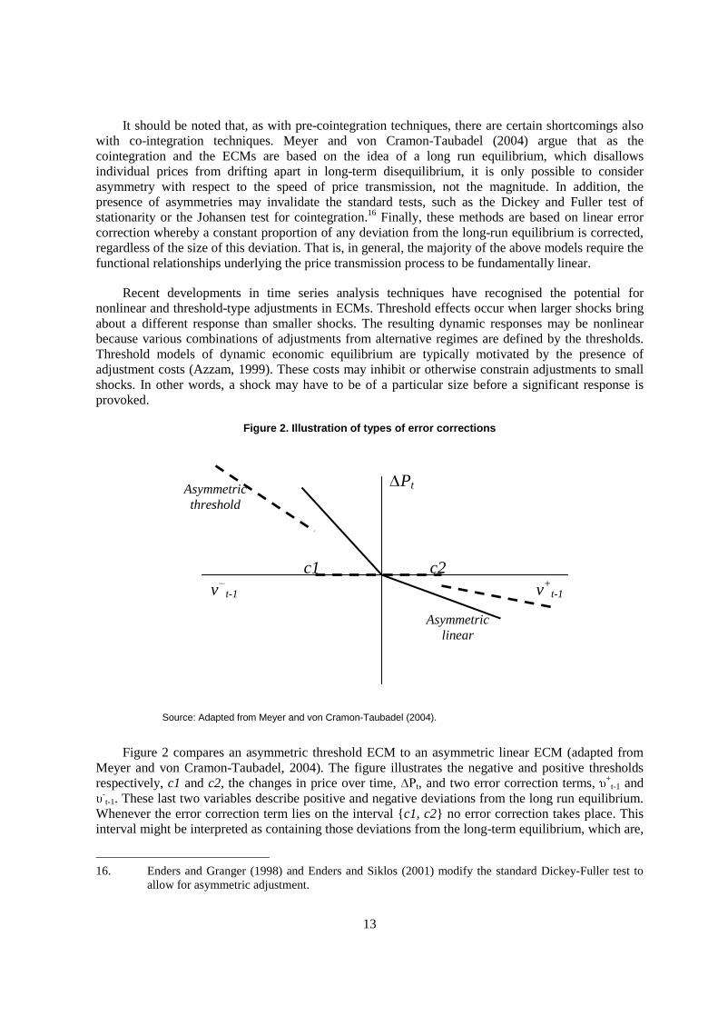
Recent developments in time series analysis techniques have recognised the potential for nonlinear and threshold-type adjustments in ECMs. Threshold effects occur when larger shocks bring about a different response than smaller shocks. The resulting dynamic responses may be nonlinear because various combinations of adjustments from alternative regimes are defined by the thresholds. Threshold models of dynamic economic equilibrium are typically motivated by the presence of adjustment costs (Azzam, 1999). These costs may inhibit or otherwise constrain adjustments to small shocks. In other words, a shock may have to be of a particular size before a significant response is provoked.

Figure 2. Illustration of types of error corrections

Source: Adapted from Meyer and von Cramon-Taubadel (2004).

Figure 2 compares an asymmetric threshold ECM to an asymmetric linear ECM (adapted from Meyer and von Cramon-Taubadel, 2004). The figure illustrates the negative and positive thresholds respectively, c1 and c2, the changes in price over time, ��t, and two error correction terms, +

t-1 and -t-1. These last two variables describe positive and negative deviations from the long run equilibrium.

Whenever the error correction term lies on the interval {c1, c2} no error correction takes place. This interval might be interpreted as containing those deviations from the long-term equilibrium, which are,

16. Enders and Granger (1998) and Enders and Siklos (2001) modify the standard Dickey-Fuller test to

allow for asymmetric adjustment.

v�t-1 v+t-1

Asymmetric threshold

c2 c1

Asymmetric linear

�Pt

14

compared to adjustment costs, so small that they will not lead to a price adjustment. It should be noted that a conventional vector error correction model is implicit within this threshold modelling framework. That is, when c1 and c2 equal zero, the threshold scheme is equivalent to a standard linear ECM.

A threshold model allows for several types of asymmetry. The first type refers to price transmission outside of the {c1, c2} interval where slopes of the corresponding line segments can differ (Figure 2), reflecting an asymmetry with respect to the speed of transmission. The second type of asymmetry refers to the fact that c1 need not equal c2. If this type of asymmetry holds, then deviations in the positive and negative directions must reach different magnitudes before a response is triggered. Indeed it is possible to use this model to explore a third type of asymmetry, namely that price shocks across levels in the marketing chain have different effects depending on the level at which the initial shock takes place.

Tong (1978) originally introduced the concept of nonlinear threshold models. Threshold modelling was initially applied to simple, univariate autoregressive models. Balke and Fomby (1997) extended the threshold autoregressive models to a co-integration framework. Their approach essentially involved specification of an autoregressive model for the error-correction term implied by a co-integration relationship. They suggested a grid search procedure whereby threshold parameters were chosen by minimizing a sum of squared errors (SSE) criterion. Threshold error correction models are a relatively recent addition to techniques for estimating asymmetric price transmission, although there have been a number of applications. For example, Goodwin and Holt (1999) estimate a full vector error correction (VEC) model of monthly beef price relationships at the farm, wholesale and retail levels. This line of research was later extended to investigate hog price relationships by Goodwin and Harper (2000), and Goodwin and Piggott (2001) for corn and soybean markets in North Carolina. Abdulai (2002) applies threshold co-integration estimations in the study of a relationship between retail and producer prices of pork in Switzerland. Serra and Goodwin (2003) studied price transmission in the Spanish dairy sector. Brooks and Melyukina (2004) estimate horizontal price transmission (between world and domestic markets) for several Brazilian commodities. Balcombe (2003) analyses threshold effects in price transmission for Brazilian wheat, maize and soya prices.17 Aguero (2004) uses a threshold error correction model to estimate asymmetric price adjustments under risk in Peruvian agricultural markets.18

Estimation of asymmetric price transmission using a threshold vector error correction model

The empirical analysis proposed in this study follows the threshold ECM of the form presented by Goodwin and Holt (1999), Goodwin and Harper (2000) and Goodwin and Piggott (2001). This model nests many other specifications and allows for a consideration of the extent and timing of the transmission of shocks, as well as for testing for any asymmetries in transmission patterns. A description of the model and a discussion of methods proposed to estimate the threshold models are presented in Annex 2.

17. Balcombe (2003) uses Classical and Bayesian techniques in estimating threshold ECM and discusses

the advantages and disadvantages of both approaches.

18. This method is extensively used outside agricultural economics, such as financial market analysis. Threshold vector ECMs are typically used to assess the effects of transaction costs in financial market, and their impacts on interest or exchange rate movements. For examples, see Seo (2003), Tkacz (2001), and Jamaleh (2002).

15

As noted above, threshold models may provide important insights, but they are relatively difficult to apply. Standard statistical software packages do not yet contain programmed procedures to estimate asymmetric price transmission with thresholds. A programme that automates, to a certain extent, estimation of one or several price time series is described in Annex 3. The program, once executed for given data, provides relevant output statistics, tests, estimated coefficients and plots of the impulse response functions (Annex 1). The programme code itself is available from the Secretariat upon request.

The estimation strategy can be summarized as follows. First, Augmented Dickey-Fuller unit root tests and Johansen co-integration tests are used to evaluate the time-series properties of the data. These tests are useful for the purpose of putting the results into the context of the larger body of research based on such tests in order to consider price transmission. The procedure then follows the general two-step approach of Engle and Granger (1987): first, a co-integrating relationship among the variables is estimated by ordinary least squares (OLS); and, second, the ECM is specified by using lagged residuals from the co-integrating regression as error correction terms. When residuals are used, the results may be sensitive to the normalization rule or method; results may not be unaffected by choices as to which of the variables is chosen as the left-hand-side variable in the co-integration regression.

A two-dimensional grid search is then conducted to define two thresholds. The procedure searches for the first threshold between 1% and 99% of the largest (in absolute value) negative error correction term. In like fashion, it searches for the second threshold between 1% and 99% of the largest positive error correction term. The error correction model is then estimated conditional on the threshold parameters. As parameter estimates for non-structural models of this sort are typically of limited interest in and of themselves, it is common to use impulse responses or dynamic multipliers to evaluate short-run and long-run effects of shocks. In contrast to the linear model case, the response to a shock in a non-linear model is dependent upon the history of the series. In addition, the possibly asymmetric nature of responses implies that the size, timing, and sign of the shock will influence the nature of the response.

In this light, there are many different possible impulse response functions. It is typical to choose a single observation or, alternatively, to calculate impulses at all observations and present the average or some other summary of the responses. The nonlinear impulse response function approach of Potter (1995) is used in this study (Annex 1). It should also be noted that, in light of the non-stationary nature of most price data and the error correction properties of a system of equations, shocks may elicit either transitory or permanent responses. In particular, non-stationarity implies that shocks may permanently alter the time path of variables.

Asymmetric price transmission ��������������������� �

In this section, the above proposed method to estimate asymmetric price transmission is illustrated empirically for a small set of commodities. For the analysis monthly price data for U.S. farm, wholesale, and retail markets were collected for beef, chicken and eggs from published USDA sources. In particular, selected versions of the Red Meats Yearbook and the Poultry Yearbook were used to obtain data concerning national average prices. The beef prices cover the period of January 1974 through December 2001. The chicken prices cover the period from January 1980 through December 2002. The egg prices cover the period from January 1972 through December 2002. Farm-level prices were quoted at direct markets. Wholesale prices were for boxed beef cut-outs. Retail prices are averages taken from the US Bureau of Labor Statistics. All prices are in US cents per pound.

16

Figures A4.1 to A4.3 in Annex 4 show the data plots for these time series. The left hand panel of each figure illustrate the prices in levels while the right hand panel shows the evolution of price indices on the basis of the first observation being equal to one. Clearly, the evolution of prices differs by commodity and by market level. Variability in prices is much higher for egg prices compared to chicken and especially beef prices. It is interesting to note that retail prices of beef appear to drift apart from those at wholesale and farm level. This evolution is, in particular, apparent when looking at the price index series which shows an almost identical evolution of wholesale and farm level prices with the retail price index trending systematically higher.

The data for chicken show retail prices following a much smoother pattern of change when compared to those at wholesale and farm level. Contrary to beef, the chicken retail price index often falls below that at the wholesale and retail levels and it is not until late 1990 that it stays systematically above these prices. In the case of egg prices there seems to follow an erratic, yet, similar pattern with the retail price index to some extent below the indices at wholesale and farm level. However, as mentioned earlier, it is very important to distinguish between analyses of margins over time per se and the price transmission along the supply chain. That is, increasing marketing margins over time do not necessarily mean presence of imperfect price transmission. In other words, margins could be increasing even under full price transmission conditions. Again, this paper does not address the issue of market power in supply chains; the main question it seeks to answer is how quickly and to what extent prices are transmitted up and down the supply chain.

The empirical application of testing for the thresholds and asymmetric price responses follow the description of the procedure in Annex 3 and uses the threshold vector error correction model defined in Annex 2. A logarithmic transformation of variables is applied for all prices, such that results may be interpreted in percentage change terms. All tables with test statistics and impulse response diagrams are reported in Annex 5. Augmented Dickey-Fuller unit root tests and Johansen co-integration tests were used to evaluate the time-series properties of the data. As noted above, to the extent the data are characterized by thresholds or other nonlinearities, these test results may not be fully reliable. These tests are useful for the purposes of putting the results into the context of the larger body of literature that has used such tests to consider price linkages. The results presented in Table A5.1 in Annex 5 are somewhat mixed. Based on the Dickey Fuller test, beef prices appear to be non-stationary while the price series for chicken and eggs are largely stationary. The results for the Johansen co-integration tests for each commodity are presented in Table A5.2. The table reports the trace test statistics and the 5% critical values for the presence of co-integration. In every case, the results are consistent with one or two co-integrating vectors among the three prices. In the case of beef, the results are consistent with three co-integrating vectors

Table A5.3 presents OLS estimates of the co-integrating relationship regressions. The co-integration relationships were normalized on the retail price, such that retail prices were regressed on wholesale and farm-level prices. The results are surprising in that the coefficients on farm prices for both beef and chicken are negative. This is in contrast to the results obtained using weekly beef price data over the 1981-1998 period by Goodwin and Holt (1999). Differences between the beef results and those presented by Goodwin and Holt (1999) might be the outcome of differences in the time periods considered, the use of monthly instead of weekly data, and different definitions of prices. The impacts on the results of the last two differences are probably of minor importance, as very similar results to those presented by Goodwin and Holt (1999) follow from estimates of the beef model for the 1981-1998 period.

Nevertheless, the differences between the estimated coefficients over the two periods remains an important issue. These may be suggestive of a considerable degree of multi-collinearity among the individual price series. Alternatively, the differences may reflect the potential for considerable

17

structural change in the data underlying the estimates. These industries have experienced substantial changes in structure, especially with regard to the level of industry concentration, over the period of study. In particular, the industries have become considerably more concentrated and the chicken and egg industries have become much more dependent upon contract production and vertical integration. Ideally, one would want to either concentrate the analysis on a shorter period for which stability is thought to exist or would want to incorporate any structural change into the models directly. A vast literature has addressed issues pertaining to the identification and testing of structural changes. In that threshold models share many of the same characteristics of structural change models (i.e. endogenous changes in parameters that imply multiple regimes), it is difficult if not impossible to identify both phenomena at once.19

Another important issue that should be noted here is that a researcher must give some thought to the timing of the relationships under consideration. If one believes that adjustments to shocks take place within a year, the use of annual data may not reveal the important dynamics of interest. Likewise, some relationships may be more accurately modelled using weekly rather than monthly price data. Of course, weekly price data are often rare and thus one must balance data availability issues against modelling considerations.

Threshold testing results and summary statistics are presented in Table A5.4. In every case, the sup(LR) tests of threshold effects imply statistically significant differences in parameters over the alternative regimes. In the case of chicken and egg markets, the majority of observations lie between the two thresholds. In the case of beef, a significant proportion of the observations lies above the upper threshold. This may be consistent with a case of structural shifts, especially in cases where the shifting across regimes appears to coincide with time. As previously noted, however, additional analysis is needed to evaluate the extent to which the results correspond to structural changes.

Table A5.4 also reports the individual threshold parameters. Although a direct interpretation of the thresholds is somewhat opaque, they represent values of the residual term from the co-integrating regression (which represent deviations from equilibrium relationships among farm, wholesale, and retail prices) that trigger changes in patterns of responses to shocks. In that the co-integrating relationship is normalized on the basis of logarithmic transformations of retail prices, the thresholds can be interpreted as the value of shocks, expressed in terms of percentage changes to the prices of a product in retail markets that will move the system to a different regime, thus implying a change in the patterns of adjustment. For example, in the case of beef the lower threshold of -0.13 corresponds to the minimum percentage deviation in the retail price needed for the price transmission realisation to move to a different regime. In the beef case, the positive threshold (+0.002%) is lower than a negative threshold (-0.13%) which could be interpreted that it is more costly to adjust to negative shocks than to positive shocks.

The logic underlying the threshold approach is that there may be certain technological relationships inherent in the price linkages and it may be costly to change these relationships for small deviations from equilibrium. However, large shocks may make it advantageous to make adjustments in the marketing and processing techniques that link farm, wholesale, and retail markets. If a shock is large enough to merit such adjustment in light of what may be substantial adjustment costs, an

19. The tests commonly used to identify structural changes with unknown break-points (Chow-type tests)

are identical to those used to test for threshold behavior (Hansen’s tests). It is incumbent upon the analyst to be cognizant of the potential for structural change as well as other structural characteristics of the industry and markets being evaluated. Without such comprehension, it is difficult to interpret the findings of empirical analysis.

18

alternative relationship among the prices may be implied. Likewise, large positive deviations may suggest adjustments that differ from large negative deviations.

In such non-structural models, individual coefficients typically have little meaning in and of themselves.20 Perhaps the best way to interpret the implications of the models for patterns of price transmission, causality, and adjustment is to consider the time paths of prices after exogenous shocks; in other words, impulse responses. The impulse responses represent percentage changes in prices to a certain percentage shock in one of the prices. As noted above, the patterns of adjustment may imply permanent changes, which is consistent with the non-stationary nature of the data, or transitory changes. The shock (impulse) that initiates the responses represents a one-time, permanent change in the variable being shocked. Note again that the nonlinear nature of the models implies that the nature of the response is dependent upon the timing, direction, and size of the shock. This follows from the fact that a shock to a price at a particular time may move the pattern of adjustment across different regimes. Shocks equivalent in size to one standard deviation of the error correction term are applied to the last observation in each market. Figures 1–27 contain illustrations of the impulse response functions. In each case, the positive and negative impulses are plotted together. To the extent that these impulses differ from one another, asymmetries are implied.

Figures 1-9 contain impulse responses for the beef market. In the case of retail and wholesale price responses to shocks, significant asymmetries are apparent, both in terms of speed and magnitude of the adjustment. In the case of farm prices, the responses appear to be much more symmetric. Retail prices appear to exhibit permanent adjustments in response to retail price shocks. In contrast, retail price adjustments in response to shocks to farm and wholesale prices are of a more transitory nature, although the adjustments take nearly two years to be complete. Wholesale prices exhibit interesting short run dynamics in response to shocks, with considerable variability being displayed in the periods immediately following the shocks. As noted, farm prices exhibit much more symmetric responses to positive and negative shocks. In accordance with the conclusions of earlier research, the responses of farm prices to shocks appear to be much more modest (as is indicated by the scale of the adjustment on the vertical axis of the diagrams). This finding is in agreement with the literature that has examined beef price adjustment and indicates much less adjustment at the farm level to wholesale and retail shocks than is the case for wholesale and retail markets.

Impulse responses for shocks to retail, wholesale, and farm level prices in the chicken market are illustrated in Figures 10-18. The impulse responses for retail prices show very different reactions to negative shocks than to positive shocks. In the case of positive shocks, retail prices show little reaction. In contrast, negative shocks trigger substantial adjustments, with considerable variability in the short run responses. It appears to take about 12-15 months for the response to shocks to settle to new long-run equilibrium values. Similar patterns are apparent in the wholesale price responses, which also exhibit a significant degree of asymmetry. In the case of farm price responses to shocks at the retail and wholesale levels, the adjustments appear again to be much more symmetric. In contrast to beef prices, a substantial degree of adjustment in farm prices occurs in reaction to shocks to prices in wholesale and retail markets. The adjustment appears to occur much more rapidly, with permanent shifts appearing to be complete after 4-6 months. These results would seem to indicate that farm-level chicken prices are much more responsive to shocks at retail and wholesale levels than is the case for beef. However, the caveats noted above regarding the potential for structural change in the underlying economic relationships being modelled are again worth repeating. 20. An exception to this statement often exists for the coefficients on the error correction terms. The

extent to which these coefficients have strong and statistically significant effects is relevant to patterns of causality and the extent to which shocks to equilibrium conditions are eliminated in the long-run. These patterns will be reflected in the impulse response analysis as well.

19

Finally, egg price impulse responses are presented in Figures 19-27. In contrast to the case of beef and chicken prices, the adjustments appear to be much more symmetric. In the case of retail prices, a considerable period of adjustment following market shocks is apparent, with price adjustments appearing to persist for 12 months or more. In the case of wholesale prices, the adjustments appear to be much faster, with new price levels being reached in 3-4 months. The duration of adjustments for farm prices is somewhere in between the two, with prices settling at new levels in 6-8 months after the shocks.

In summary the application of the threshold vector error correction model to retail, wholesale, and farm level prices in the U.S. beef, chicken, and egg markets indicates the presence of asymmetries in responses to negative and positive price shocks. Impulse response diagrams illustrate responses to shocks, with some shocks producing short-lived, temporary adjustments and others producing permanent market adjustments. Concerns have been raised of the potential for structural changes to be inherent in the underlying economic relationships in these markets. In particular, these markets have undergone significant structural adjustments that were brought about by significant increases in the concentration of the industries and, in the case of chicken and egg markets, by much greater vertical integration. 1

Conclusions

The objective of this paper is to introduce the subject and mechanisms of asymmetric price transmission, and to discuss a relatively new procedure that measures price transmission empirically. The focus is on vertical price transmission, i.e. along the supply chain, and the possible types of adjustments to a price shock are discussed. In particular, it was noted that vertical price adjustments can be characterised by the speed, direction and magnitude relative to the initial market shock, with the results in each case being determined by the underlying relationships among agents at different levels of activity.

The review of the literature reveals that market power is often perceived as the main potential cause of asymmetric price transmission, although other possible causes for imperfect price pass through are discussed. The most important alternative explanations for any finding of asymmetry are the presence of adjustment and menu costs. The presence of government interventions was also identified in the literature as a possible cause of price asymmetry. The paper points out the importance of adjustment costs that may be high enough to completely inhibit market adjustments to small price changes and, consequently, prohibit the transmission of these changes across market levels. The discussion of empirical findings in the literature limits itself to research that studied asymmetric price transmission for agricultural commodities and provides often mixed evidence. Unclear or even conflicting results point to the complexity of the price transmission phenomenon and prompt for further research.

The discussion of empirical methods to estimate price transmission concentrates on both well established and relatively new techniques. In particular, pre-cointegration and cointegration methods are reviewed with particular attention paid to a recent introduction of threshold vector error correction models. The latter models nest many other specifications and allow for a consideration of the extent and timing of the transmission of shocks, as well as for testing for any asymmetries in transmission patterns. The threshold vector error correction models also allows for nonlinearities in cases where prices at one level adjust to price changes elsewhere in the supply chain only if the deviation exceeds a specific positive and negative “threshold” levels. The thresholds are relevant for price changes in either direction, and may differ for rising and falling prices. A price change in the one level that falls in the interval between the negative and positive thresholds leads to no adjustment in price at the other

20

level. Once these thresholds are exceeded, the magnitude of the price change outweighs the transaction costs of changing prices at the other level; agents implement price changes and price transmission takes place.

This method is applied to retail, wholesale and farm level prices of the U.S. beef, chicken and egg markets for illustrative purposes. The results indicate significant asymmetries in responses to negative and positive price shocks. The asymmetries are apparent both in terms of speed and magnitude of the adjustment. Impulse response diagrams illustrated different responses to shocks by market level and commodity, with some shocks producing short-lived, temporary adjustments and others producing permanent market adjustments.

21

REFERENCES

Abdulai, A. (2002). “Using threshold co-integration to estimate asymmetric price transmission in the Swiss pork market” Applied Economics, 34, 679-687.

Aguero, J. (2004). “Asymmetric price adjustments and behaviour under risk: Evidence from Peruvian agricultural markets”, Selected Paper prepared for presentation at the American Agricultural Economics Association Annual Meeting, Denver, Colorado, July 1-4, 2004.

Aguiar, D. and J.A. Santana, (2002). “Asymmetry in Farm to Retail Price Transmission: Evidence for Brazil,” Agribusiness, 18 (2002): 37-48.

Ardeni, P.G. (1989). “Does the Law of One Price really hold for commodity prices?” American Journal of Agricultural Economics, 71: 303-328.

Azzam, A. M. (1999). “Asymmetry in rigidity in farm-retail price transmission”, American Journal of Agricultural Economics, 81, 525–533.

Baffes J. and M. Ajwad, (2001). “Identifying price linkages: a review of the literature and an application to the world market of cotton”, Applied Economics, 33: 1927-1941.

Baffes, J. (1991). “Some further evidence on the Law of One Price”, American Journal of Agricultural Economics, 4: 21-37.

Bailey, D. V. and B. W. Brorsen, (1989). “Price Asymmetry in Spatial Fed Cattle Markets,” Western Journal of Agricultural Economics. 14:246-52.

Balcombe K. (2003). Threshold Effects in Price transmission: The case of Brazilian Wheat, maize and Soya Prices. Consultancy paper provided to the OECD Secretariat.

Balke, N. S. and T. B. Fomby, (1997). “Threshold Cointegration," International Economic Review. 38:627-645.

Balke, N.S., Brown, S.P.A. and M.K. Yücel, (1998) “Crude Oil and Gasoline Prices: An asymmetric Relationship?”, Federal Reserve Bank of Dallas, Economic Review, 2-11.

Ball, L. and N. G. Mankiw, (1994). “Asymmetric Price Adjustment and Economic Fluctuations,” Economic Journal 104:247-261.

Barrett, C.B. (2001). “Measuring integration and efficiency in international agricultural markets”, Review of Agricultural Economics, 23: 19-32.

Benson, B. L. and Faminow, M. D. (1985). “An alternative view of pricing in retail food markets”, American Journal of Agricultural Economics, 67, 296–305.

Bernard, J.C. and L.S. Willett, (1996). “Asymmetric Price Relationship in the U.S. Broiler Industry,” Journal of Agricultural and Applied Economics, 28: 279-289.

Bettendorf, L. and Verboven, F. (2000). “Incomplete transmission of coffee bean prices in the Netherlands”, European Review of Agricultural economics, 27, 1-16.

Blauch, B. (1997). “Testing for food market integration revisited”, Journal of Development Studies, 33: 477- 487.

Blinder, A.S. (1982). “Inventories and Sticky Prices: More on the Microfoundation of Macroeconomics”, American Economic Review, 72(3): 334-348.

Blinder, A. S. (1994). “On Sticky Prices: Academic Theories Meet the Real World.” In Monetary Policy, ed. N. G. Mankiw, Chicago: University of Chicago Press.

22

Blinder, A. S., E. R. Canetti, D. E. Lebow, and J. B. Rudd, (1998). Asking About Prices: A New Approach to Understanding Price Stickiness. New York: Sage Foundation.

Borenstein, S., Cameron, A.C. and R. Gilbert, (1997). “Do Gasoline Prices respond asymmetrically to Crude Oil Price Changes?”, Quarterly Journal of Economics, 112: 305-339.

Boyd, M. S. and B. W. Brorsen, (1988). “Price Asymmetry in the U.S. Pork Marketing Channel,” North Central Journal of Agricultural Economics 10: 103-110.

Brooks, J. and Melyukina, O. (2003) Estimating the Pass-Through of Agricultural Policy Reforms: An Application to Russian Crop Markets with Possible Extensions, Contributed Paper, International IATRC Conference, Capri, Italy, 23-26 June, 2003.

Brooks, J. and Melyukina, O. (2004) Estimating the Pass-Through of Agricultural Policy Reforms: an Application to Brazilian Commodity Markets, OECD World Outlook Group Meeting, São Paolo, Brazil, 24-25 May 2004.

Bunte, F.H.J. and E. Kuiper, (2003), Market power in food chains. Paper for EUNIP. Porto, 19 September 2003.

Capps Jr., O. and P. Sherwell, (2005). “Spatial Asymmetry in Farm-Retail Price Transmission Associated with Fluid Milk Products”, Selected Paper prepared for presentation at the American Agricultural Economics Association Annual Meeting, Providence, Rhode Island, July 24-27, 2005.

Chevalier, J., Kashyap, A. and P.E. Rossi, (2003). “Why Don't Prices Rise during Periods of Peak Demand? Evidence from Scanner Data”, American Economic Review, 93 (1): 15-37.

Cotterill, R.W. (2002). Who Benefits from Deregulated Milk Prices: The Missing Link is the Marketing Channel. Food Marketing Policy Issue Paper No. 26 April 2002 Food Marketing Policy Center, Department of Agricultural and Resource Economics, University of Connecticut.

Cowling, K., and M. Waterson (1979), “Price-cost margins and market structure”Economica, 43: 267-274.

Dickey, D. and W.A. Fuller, (1979). “Distribution of the Estimates for Autoregressive Time Series with a Unit Root”, Journal of the American Statistical Association, 74: 427-431.

Dickey, D. and W.A. Fuller, (1981). “Likelihood Ratio Tests for Autoregressive Time Series with a Unit Root”, Econometrica, 49: 1057-1072.

Dornbusch, R. (1987). “Exchange rates and prices”, American Economic Review, 93-106.

Enders, W. (2004). Applied Econometric Time Series, John Wiley and Son.

Enders, W. and C.W.J. Granger, (1998). “Unit-root tests and Asymmetric Adjustment with an example using the term structure of interest rates”, Journal of Business and Economic Statistics, 16: 304-311.

Enders, W. and P.L. Sicklos, (2001). “Cointegration and Threshold Adjustment”, Journal of Business and Economic Statistics, 199: 166-176.

Engle, R. F. and C. W. J. Granger, (1987). “Cointegration and Error Correction: Representation, Estimation, and Testing,” Econometrica. 55: 251-276.

FAO (2003). “Market integration and price transmission in selected Food and cash crop markets of developing countries: Review and applications”, by Rapsomanikis, G., Hallam, D., and P. Conforti, in Commodity Market Review 2003-2004., Commodities and trade division, FAO, Rome.

Frost, D. and R. Bowden, (1999). “An Asymmetry Generator for Error-Correction Mechanisms, with Application to Bank Mortgage-Rate Dynamics”, Journal of Business and Economic Statistics, 17(2): 253-263.

Gardner B.L. and K.M. Brooks, (1994). “Food prices and market integration in Russia: 1992-93”, American Journal of Agricultural Economics, 76: 641-646.

Gardner, B.L. (1975). “The Farm-Retail Price Spread in a Competitive Food Industry”, American Journal of Agricultural Economics 57, 383-406.

23

Girapunthong, N., J. J. VanSickle, and A. Renwick, (2003). “Price asymmetry in the United States fresh tomato market”, Journal of Food Distribution Research 34(3): 51-59.

Gohin, A. and Guyomard, H. (2000). “Measuring market power for food retail activities: French evidence”, Journal of Agricultural Economics, 51, 181-195.

Goodwin B.K. and D. C. Harper, (2000). “Price transmission, threshold behaviour, and Asymmetric Adjustment in the US pork sector.” Journal of Agricultural and Applied Economics, 32: 543-553.

Goodwin, B. K. and M. T. Holt. (1999). “Asymmetric Adjustment and Price Transmission in the U.S. Beef Sector,” American Journal of Agricultural Economics. 79: 630-637.

Goodwin, B. K. and N. Piggott, (2001). “Spatial Market Integration in the Presence of Threshold Effects,” American Journal of Agricultural Economics, 83: 302-17

Granger, C. W. J. and P. Newbold, (1974). “Spurious Regressions in Econometrics”, Journal of Econometrics, 2: 111-120.

Greene, W.H. (1993). Econometric Analysis. New York, Macmillan Publishing Company.

Hahn, W.F. (1990). “Price Transmission Asymmetry in Pork and Beef Markets,” The Journal of Agricultural Economics Research, 42, 2: 21-30.

Hamilton, J.D. (1994). Time Series Analysis. Princeton: Princeton University Press.

Hansen, B. E. (1997). “Inference in TAR Models,” Studies in Nonlinear Dynamics and Econometrics. RePEc:bep:sndecm:2:1997:1:1-14

Heien, D. M. (1980). “Markup pricing in a dynamic model of the food industry,” American Journal of Agricultural Economics, 62: 11-18.

Holloway, G.J. (1991). "The Farm-Retail Price Spread in an Imperfectly Competitive Food Industry", American Journal of Agricultural Economics, 71, 979–989.

Houck, J. P. (1979). “An Approach to Specifying and Estimating Non-Reversible Functions,” American Journal of Agricultural Economics. 59: 570-72.

Jamaleh, A. (2002). “Explaining and forecasting the euro/dollar exchange rate through a non-linear threshold model”, The European Journal of Finance, 8(4): 422-448.

Johansen S. (1988). “Statistical Analysis of Cointegration Vectors,” Journal of Economic Dynamics and Control, 12: 231-254.

Kinucan, H. W. and O. D. Forker, (1987). “Asymmetry in Farm-Retail Price Transmission for Major Dairy Products,” American Journal of Agricultural Economics. 69: 307-328.

Livanis, G. and C.B. Moss, (2005). “Price Transmission and Food Scares in the U.S. Beef Sector”, Presented at the American Agricultural Economics Association Meetings in Providence, Rhode Island 2005.

Lloyd, T., McCorriston, S., Morgan, C. W. and A.J. Rayner, (2003). “The Impact of Food Scares on Price Transmission in Inter-Related Markets”, paper presented to the XXVth IAAE Conference in Durban, South Africa.

Lo, M. and E. Zivot, (2001) “Threshold Cointegration and Nonlinear Adjustment to the Law of One Price,” Macroeconomic Dynamics, December.

London Economics, (2003). Examination of UK Milk Prices and Financial Returns, Report prepared for The Milk Development Council, February.

London Economics, (2004). Investigation of the determinants of farm-retail price spreads, Final report to DEFRA, U.K.

Maddala, G.S and I. Kim, (1998). Unit roots, cointegration and structural change. Cambridge University Press.

McCorriston, S. and Sheldon, I.M. (1996). “Trade Policy in Vertically-Related Markets”, Oxford Economic Papers 48: 664-672.

24

McCorriston, S., Morgan, C. W. and Rayner, A. J. (2001). “Price transmission: the interaction between market power and returns to scale”, European Review of Agricultural Economics, 28, 143–159.

MDC (2004). Dairy supply chain margins 2003-04: Who made what in the dairy industry and how it has changed, published by Milk Development Council, UK.

Meyer, J. and S. von Cramon-Taubadel, (2004). “Asymmetric Price Transmission: A Survey,” Journal of Agricultural Economics. 55: 581-611.

Mohanty, S. and E.W. F. Peterson and N.C. Kruse, (1995). “Price Asymmetry in the International Wheat Market,” Canadian Journal of Agricultural Economics, 43: 355-366.

Peltzman, S. (2000). “Prices Rise Faster than They Fall,” Journal of Political Economy. 108: 466-502.

Potter, S. M. (1995) “A Nonlinear Approach to US GNP," Journal of Applied Econometrics. 10:109-125.

Punyawadee, V., M.S. Boyd and M.D. Faminow, (1991). “Testing for Asymmetric Pricing in Alberta Pork Market,” Canadian Journal of Agricultural Economics, 39: 493-501.

Reagan, P. and Weitzman, M. (1982). “Asymmetries in price and quantity adjustments by the competitive firm”, Journal of Economic Theory, 27, 410–420.

Sanjuán, A.I. and P. J. Dawson, (2003). “Price transmission, BSE and structural breaks in the UK meat sector”, European Review of Agriculture Economics 30 (2): 155-172.

Scholnick, B. (1996). “Asymmetric Adjustment of commercial Bank Interest Rates: Evidence from Malaysia and Singapore”, Journal of International Money and Finance, 15: 485-496.

Seo, B. (2003). “Nonlinear mean reversion in the term structure of interest rates”, Journal of Economic Dynamics and Control, 27: 2243 – 2265

Serra, T. and Goodwin, B.K. (2003). “Price transmission and asymmetric adjustment in the Spanish dairy sector”, Applied Economics, 2003, 35, 1889–1899.

Tiffin R, and Dawson P.J. (2000). “Structural breaks, cointegration and the farm retail price spread for lamb”, Applied Economics, 32, 1281-1286.

Tkacz, G. (2001). Endogenous thresholds and tests for asymmetry in U.S. prime rate movements, Department of Monetary and Financial Analysis, Bank of Canada, Ottawa.

Tong, H. (1978). On a Threshold Model in Pattern Recognition and Signal Processing. Ed. C. Chen, Amsterdam: Sijhoff and Noonhoff.

Tweeten, L.G. and C.L. Quance, (1969). “Positivistic measures of aggregate supply elasticities: Some new approaches”, American Journal of Agricultural Economics, 51: 342-352.

USDA (2004). Contracts, Markets, and Prices: Organizing the Production and Use of Agricultural Commodities by J. MacDonald, J. Perry, M. Ahearn, D. Banker, W. Chambers, C. Dimitri, N. Key, K. Nelson, and L. Southard., Economic Research Service, Report Number 837.

Von Cramon-Taubadel, S and Loy, J.-P. (1996) “Price asymmetry in the international wheat market: Comment”, Canadian Journal of Agricultural Economics, 44: 311-317.

Von Cramon-Taubadel, S. (1998). “Estimating Asymmetric Price Transmission with the Error Correction Representation: An Application to the German Pork Market,” European Review of Agricultural Economics. 25: 1-18.

Von Cramon-Taubadel, S. and Fahlbusch, S. (1994) “Identifying asymmetric price transmission with error correction models”, Poster Session EAAE European Seminar in Reading.

Von Cramon-Taubadel, S. and J. Meyer, (2001). “Asymmetric Price Transmission: Fact or Artefact? “ Paper prepared for the 71th EAAE Seminar “The food consumer in the early 21st century” in Zaragoza, Spain, 19-20 April 2001.

Wann, J.J. and Sexton. R.J. (1992). “Imperfect competition in multi-product food industries with an application to pear processing”, American Journal of Agricultural Economics, 72, 980–990.

25

Ward, R. W. (1982). “Asymmetry in Retail, Wholesale, and Shipping Point Prices for Fresh Fruits and Vegetables,” American Journal of Agricultural Economics. 62: 205-212.

Weldegebriel, H. T. (2004). “Imperfect Price Transmission: Is Market Power Really to Blame?” Journal of Agricultural Economics 55: 101-114.

Wohlgenant, M.K. (1985). " Competitive Storage, Rational Expectations, and Short-Run Food Price Determination", American Journal of Agricultural Economics, 67, 739–748.

Wohlgenant, Michael K. (2001). “Marketing Margins: Empirical Analysis,” in Bruce Gardner and Gordon Rausser, ed., Handbook of Agricultural Economics, Volume 1, Amsterdam: Elsevier Science B.V., chapter 16, pp. 934-970.

Wolffram, R. (1971). “Positivistic Measures of Aggregate Supply Elasticities-- Some New Approaches-- Some Critical Notes,” American Journal of Agricultural Economics. 53: 356-59.

Zachariasse, V. and F. Bunte, (2003). How are farmers faring in the changing balance of power along the food supply chain?, OECD Conference: Changing Dimensions of the Food Economy: Exploring the Policy Issues, The Hague, 6-7 February 2003.

Zhang, P., S.M. Fletcher and D.H. Carley, (1995). “Peanut Price Transmission Asymmetry in Peanut Butter”, Agribusiness, 11(1): 13-20.

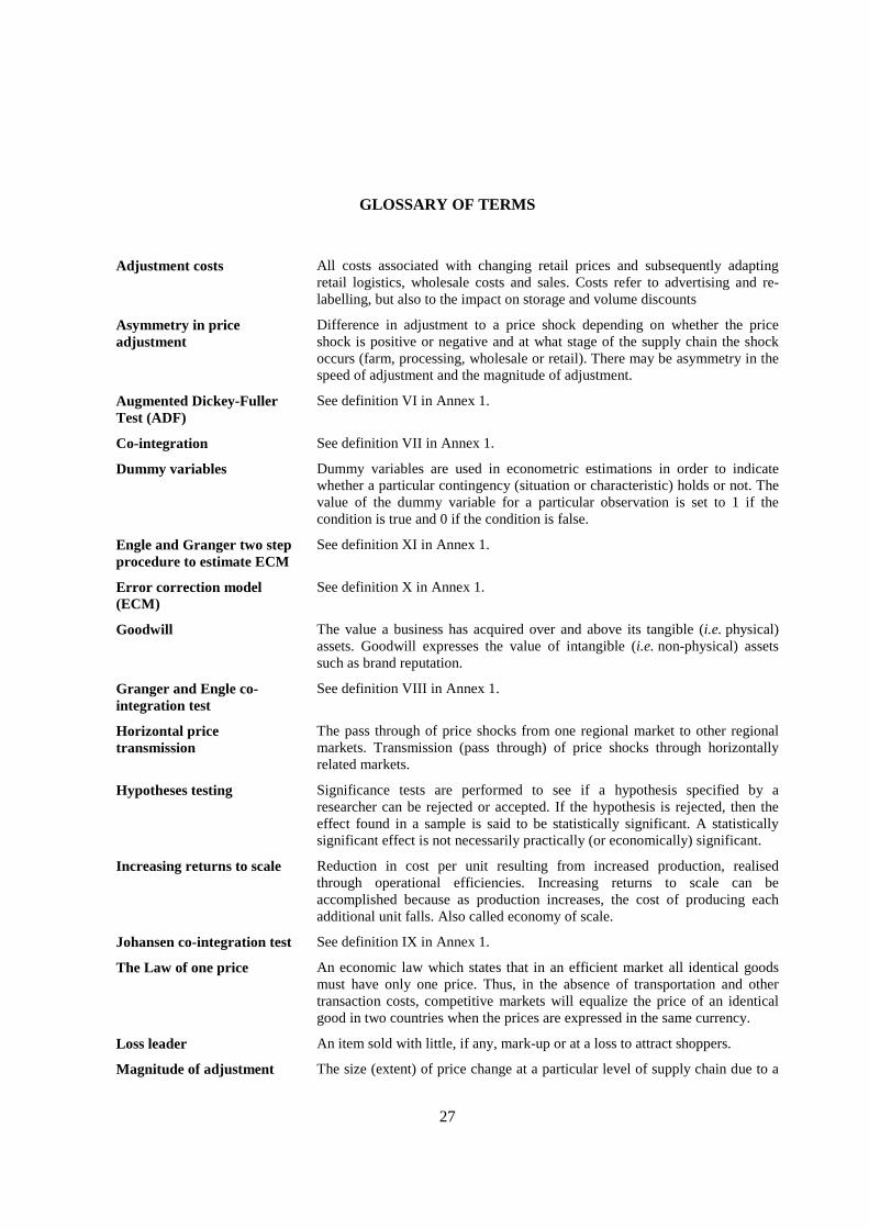
27

GLOSSARY OF TERMS

Adjustment costs All costs associated with changing retail prices and subsequently adapting retail logistics, wholesale costs and sales. Costs refer to advertising and re-labelling, but also to the impact on storage and volume discounts

Asymmetry in price adjustment

Difference in adjustment to a price shock depending on whether the price shock is positive or negative and at what stage of the supply chain the shock occurs (farm, processing, wholesale or retail). There may be asymmetry in the speed of adjustment and the magnitude of adjustment.

Augmented Dickey-Fuller Test (ADF)

See definition VI in Annex 1.

Co-integration See definition VII in Annex 1.

Dummy variables Dummy variables are used in econometric estimations in order to indicate whether a particular contingency (situation or characteristic) holds or not. The value of the dummy variable for a particular observation is set to 1 if the condition is true and 0 if the condition is false.

Engle and Granger two step procedure to estimate ECM

See definition XI in Annex 1.

Error correction model (ECM)

See definition X in Annex 1.

Goodwill The value a business has acquired over and above its tangible (i.e. physical) assets. Goodwill expresses the value of intangible (i.e. non-physical) assets such as brand reputation.

Granger and Engle co-integration test

See definition VIII in Annex 1.

Horizontal price transmission

The pass through of price shocks from one regional market to other regional markets. Transmission (pass through) of price shocks through horizontally related markets.

Hypotheses testing Significance tests are performed to see if a hypothesis specified by a researcher can be rejected or accepted. If the hypothesis is rejected, then the effect found in a sample is said to be statistically significant. A statistically significant effect is not necessarily practically (or economically) significant.

Increasing returns to scale Reduction in cost per unit resulting from increased production, realised through operational efficiencies. Increasing returns to scale can be accomplished because as production increases, the cost of producing each additional unit falls. Also called economy of scale.

Johansen co-integration test See definition IX in Annex 1.

The Law of one price An economic law which states that in an efficient market all identical goods must have only one price. Thus, in the absence of transportation and other transaction costs, competitive markets will equalize the price of an identical good in two countries when the prices are expressed in the same currency.

Loss leader An item sold with little, if any, mark-up or at a loss to attract shoppers.

Magnitude of adjustment The size (extent) of price change at a particular level of supply chain due to a

28

shock of a certain size at another level of supply chain.

Market power An ability of a firm (or group of firms) to raise and maintain price above the level that would prevail under perfect competition.

Marketing Margin Difference between prices at different levels of marketing system. (also called farm-retail price spread or marketing cost).

Menu costs All costs associated with changing retail prices. Costs refer to advertising and re-labelling. Menu costs are thought to be fixed: they are the same for small and large changes.

Nature of adjustment An adjustment following a positive or negative shock.

Negative shock An event that suddenly decreases the price of a product at a particular level of supply chain.

Non-linear impulse response functions

See definition XIII in Annex 1.

Oligopoly A market structure in which only a few sellers offer similar or identical products.

Oligopsony A market in which only a few buyers demand similar or identical products.

Positive shock An event that suddenly increases the price of a product at a particular level of supply chain.

Purchasing power parity (PPP)

The exchange rate between two countries that is equal to the ratio of the price levels in these countries of a fixed basket of goods and services.

Speed of adjustment The time lag needed for a shock at one level of supply chain to be transmitted (partially or fully) to another level of supply chain.

Standard deviation The standard deviation is the square root of the variance (see Variance). Unlike the variance, which is a somewhat abstract measure of variability, the standard deviation can be readily conceptualized as a distance along the scale of measurement.

Stationarity See definition III. in Annex 1.

Threshold level Small price changes produce more costs than benefits (see Menu costs). The threshold level refers to the smallest price change for which benefits exceed costs and price adjustment actually takes place. There may be a different threshold for price decreases and price increases.

Threshold vector error correction model

See Annex 2.

Time series See definition I in Annex 1.

Unit Root See definition IV in Annex 1.

Vertical price transmission A pass through of price shocks along the supply chain. The adjustment to a price shock occurring at one stage of the supply chain to all other stages, e.g. from producer to wholesale and to retail levels, or vice versa

Variance A measure of the distribution around a mean. It is computed as the average squared deviation of each number from its mean. For example, for the numbers 1, 2, and 3 the mean is 2 and the variance is:

( (1-2)2 +(2-2)2 + (3-2)2 ) / 3 = 0.667.

29

Annex 1. Time Series Analysis – Brief Overview

The annex presents some of the basic concepts and definitions related to estimation and testing for price transmission in the time series. An interested reader is recommended to consult the numerous econometric books that explore in details the basics of time series analysis (Hamilton, 1994; Maddala and Kim, 1998; Enders, 2004).

I. Time series

A time series is a sequence of data points, measured typically at successive times, spaced apart at uniform time intervals (week, month, year, etc.). A typical time series may exhibit a trend, a cycle, a seasonal component, and an irregular component (random variable). The trend is the long term pattern of a time series. A trend can be positive or negative depending on whether the time series exhibits an increasing long term pattern or a decreasing long term pattern. If a time series does not show an increasing or decreasing pattern then the series is stationary in the mean. A cyclical pattern in time series is characterised by an oscillation around a given trend. Seasonality refers to a cycle which appears at a regular time (e.g. retail sales peak during Christmas, etc.). The trend in time series might be deterministic or stochastic. A deterministic trend refers to the long term trend that is not affected by short term fluctuations in the economy. The series is said to have a stochastic trend when random incidents in economy have a permanent effect on the trend.

II. Random walk model

A random walk is defined as a process where the current value of a variable is composed of the past value plus an error term defined as a white noise (a normal variable that is uncorrelated with past values and has a mean of zero). The implication of a random walk process is that the best prediction of a variable y for next period is the current value, or in other words the process does not allow to predict the change in the variable from the previous period (yt ���t-1). That is, the change of y is absolutely random. The mean of a random walk process is constant but its variance is not. As time increases the variance of yt approaches infinity. Therefore a random walk process is non-stationary.

III. Stationarity

Stationarity is defined as a quality of a process in which the statistical parameters (mean and standard deviation) of the process do not change with time. It follows that non-stationary time series or stochastic process evolves over time. It may have trends in its mean or variance. Many economic time series are non-stationary, and some transformation such as differencing or detrending is typically needed to make them stationary. In the presence of non-stationary variables, there might be what Granger and Newbold (1974) call a spurious regression. A spurious regression appears to have significant relationship among variables but the results are in fact without any economic meaning. If a time series is differenced once (by subtracting yt-1 from yt) and the differenced series is stationary, the (random walk) series is then “integrated of order 1”, denoted by I(1). In general, if a time series has to be differenced "d" times to be stationary, it is referred to as I(d). By convention, if d = 0, I(0) process represents a stationary time series.

30

IV. Unit Root

A variable is said to contain a unit root or is I(1) if it is non-stationary. The use of data characterised by unit roots may lead to serious error in statistical inference.

ttt yy �� ���1 (A1.1)

��� ������� ������������ ������������ ����������������� �������� ������������ ��� �� ������� ����becomes the random walk model), and the series is non-stationary. For a series to be stationary, � must be less than unity in absolute value. Hence stationarity requires that �1< � < 1.

V. Dickey-Fuller Unit Root Test (DF)

By subtracting yt-1 from each side of the equation A1.1 yields:

yt ���t-1 = yt-1 ���t-1 �� t (A1.2) � yt = ( -1)yt-1 �� t (A1.3) � yt = �yt-1 �� t (A1.4)

where � is the first difference operator and ���� ��1. Testing the hypothesis � = 1 is equivalent to testing the hypothesis �=0. Dickey and Fuller (1979) consider three different regression equations that can be used to test for the presence of a unit root, regressions: with no constant and trend, with constant and with constant and trend. In each case the null hypothesis is H0: �=0 (unit root). The test statistics from the testing regressions are known as the statistics critical values �, ��, and �� (the type of statistics depends whether an equation contains trend and/or intercept), which were tabulated by Dickey and Fuller (1979). The regressions provide a t-statistic of the estimated �. The t-statistic is then compared to the critical value � statistic. If t >� , H0 is rejected, it means the yt is stationary. If t <� , H0 is not rejected, it means the yt is non-stationary.

VI. Augmented Dickey-Fuller Test (ADF)

��� ������ ��� t has autocorrelation more than one period, the unit root test can be modified as

(A1.5)

The number of lagged difference terms to be included can be chosen based on t-test, F-test or the Akaike’s Information Criterion (AIC) (see Greene, 1993) The null hypothesis for the ADF is the same as the DF test (i.e., H0: �=0). To test the hypothesis the model is first run with the term �yt-1 included (so called unrestricted model RSSUR) and then without this term (so called restricted model and obtains RSSR).

The computed F-statistic )/(

/)(

knRSS

rRSSRSSF

UR

URR

��

� is then compared to the critical values that are

tabulated by Dickey-Fuller (1981). Note that n stands for a number of usable observations, r stands for

�

���������

k

ititjtt yyy

211 ����

31

a number of restrictions and k is a number of parameters estimated in the unrestricted model. Note that other possibility to test for the presence of unit root is to apply the Philips Perron test (PP) (see Maddala and Kim (1998)).

VII. Co-integration

As discussed above, the regression of non-stationary data series gives way to both spurious and inconsistent regression problems. However, in a multivariate context, there might be a linear combination of integrated variables that is stationary. Such variables are said to be co-integrated. That is, they share a common unit root and the sequence of stochastic shocks is common to both. If two non-stationary series are co-integrated then, by definition, the extent by which they diverge from each other will have stationary characteristics and will reflect only the disequilibrium. Thus co-integration is a powerful concept that allows to capture the equilibrium relationship even between non-stationary series (if such equilibrium relationship exists) within a stationary model. Co-integration implies that prices move closely together in the long run, although in the short run they may drift apart. Co-integration analysis is concerned with estimating long run economic relationships among non-stationary, integrated variables.

VIII. Granger and Engle co-integration test

Granger and Engle (1987) developed a simple procedure to test for co-integration which comprises of estimating the static co-integrating regression (A1.16) (using OLS), and applying unit root tests, such as the ADF and Phillips-Perron to the estimated residuals , in order to test the null hypothesis of no co-integration.

yt��� + xt + t (A1.6)

if y and x are I(1) then the residual t from the regression of those series would also be I(1), unless they are co-integrated. Thus if the residuals are distributed I(1) we accept the null hypothesis of non-co-integration, but if the residuals are I(0) then we reject the null and accept that y and x are co-integrated. Thus, tests for co-integration are the direct analogues of the Dickey-Fuller tests developed for the analysis of unit roots in a single data series, except that here the tests are applied to the residuals of the "co-integrating regression". Because the process of regression, by definition, minimizes the variation of the residuals around a mean of zero, the estimated residuals will be biased towards stationarity. The critical values for the DF t-test statistics used to test for co-integration are therefore higher in absolute value than those used to test the order of integration of the univariate time series. Moreover since the regression creates a mean-zero error term the DF testing equation necessarily assumes that there is no constant (drift term).

IX. Johansen co-integration test

The Johansen (1988) procedure relies on the relationship between the rank of a matrix and its characteristic roots. Enders (2004) notes that Johansen procedure could be viewed as a multivariate generalisation of the Dickey-Fuller test. Johansen suggests to start with a traditional vector autoregressive model (VAR), to select appropriate number of lags based on the likelihood ratio test or alternatively AIC statistics, to estimate the vector error correction model and determine the rank of the matrix of parameters (see Enders 2004). The co-integration of the system is tested using the maximum likelihood Lmax(r) which is a function of the cointegration rank r. Johansen describes two test methods: (1) Trace Test and (2) Maximum Eigenvalue Test.

32

The trace test is based on the log-likelihood ratio ln[Lmax(r)/Lmax(k)], and is conducted sequentially for r = k-1,...,1,0. The trace test tests the null hypothesis that the cointegration rank is equal to r against the alternative that the cointegration rank is k. The latter implies that Xt is trend stationary.

The maximum Eigenvalue test is based on the log-likelihood ratio ln[Lmax(r)/Lmax(r+1)], and is conducted sequentially for r = 0,1,..,k-1. The test tests the null hypothesis that the co-integration rank is equal to r against the alternative that the co-integration rank is equal to r+1.

X. Error correction model (ECM)

An error-correction model is a dynamic model in which the movement of the variables in any periods is related to the previous period’s gap from long-run equilibrium. Co-integration provides a means of partitioning the evolution of time-series data into its two components (i.e. he long-run equilibrium characteristics and the short-run disequilibrium dynamics) using a direct link between co-integration and the so-called error correction model (ECM). This link is formalized in the Engle-Granger Representation Theorem which states that if two series are co-integrated then they will be most efficiently represented by an error correction specification. Furthermore, if the series is co-integrated, and the ECM validated, then it will encompass any other dynamic specification - such as the partial adjustment mechanism. For any set of I(1) variables, error correction and co-integration are equivalent representations. Thus a specification of ECM is the most efficient way of representing the long-run or equilibrium properties of the system, the short-run or disequilibrium properties and the nature of the adjustment towards equilibrium.

XI. Engle and Granger two step procedure to estimate ECM

Engle and Granger (1987) proposed a relatively simple two step procedure to estimate an error correction model. In the first step the static co-integrating regression (using OLS) is estimated as in A1.6 and tests for the presence of co-integration are carried out as described above. If co-integration is accepted, then A1.6 is said to describe the long-run relationship between y and x and the parameter vect��� �� ����������� ����� ���co-integrating vector. In the second step the residuals saved from the OLS first step estimation of the long-run equilibrium are used in the error correction model

�yt = � xt + ^

t-1 + et (A1.7) where ^

t-1 = ( yt-1 �^�� ^ xt-1 ).

It should be noted a drawback of the Engle-Granger two-step procedure is that when residuals are used, the results may be sensitive to the normalization rule (i.e. by which of the variables is chosen as the “left-hand-side variable in the cointegration regression). That is the results could indicate that the variables are co-integrated using one variable for the normalisation but are not co-integrated using another variable for the normalisation. In such circumstances it is possible that only subsets of the variables are co-integrated.

XII. Illustration of a test for asymmetric price transmission based on ECM

Von Cramon-Taubadel and Fahlbusch (1994) were among the first to incorporate the concept of co-integration into models of asymmetric price transmission. In brief, in their approach a standard error correction model (ECM) is extended by the incorporation of asymmetric adjustment terms. The procedure involves estimating a relationship between prices (for example retail and farm-level) by ordinary least squares (OLS) and testing for the presence of a spurious regression. If the prices can be

33

referred to as being co-integrated the estimated coefficient of the OLS is an estimate of the long-term equilibrium relationship between them. In a second step, an ECM is estimated. The model includes a so called error correction term which measures deviations from the long run equilibrium between the two prices. The inclusion of this term allows the estimated price to respond to the changes in the explanatory price but also to correct any deviations from the long run equilibrium that may be left over from previous periods. Splitting the error correction term positive and negative components makes it possible to test for APT. The ECM takes to following form:

(A1.8) where Pt

1 and Pt2 are two vertically related prices (i.e. retail and farm-level), �� ��� ��� ���������

indicator (differencing means subtracting Pt-1 from Pt��� j����� ���� ����� ��� ����������� ������ +t-1

���� -t-1 are the positive and negative deviations from the long run equilibrium.

XIII. Non-linear impulse response functions

An impulse response function traces out the response of a variable of interest to an exogenous shock. Often the response is portrayed graphically with horizon on the horizontal axis and response on the vertical axis. In a linear model, the impulse responses are not history dependent and the magnitude of the shock does not alter the time-profile of the responses. Moreover, the effects of a two unit shock are simply twice those for the one-unit shock and the effects of a negative shock are simply the negative of those for positive shock (see Enders 2004 for detailed explanations). However, the interpretation of impulse response functions for a nonlinear model is more difficult as the impulse responses are history dependent. That is the effect of a shock on the time path depends on the magnitudes of the current and subsequent shocks and the sign of the shock can matter.

Potter (1995) notes that in nonlinear models for any specific history the effect of shocks of varying magnitudes and signs is not a simple scaling of a unit shock and that for the same shock but different histories the response can differ markedly. Potter (1995) defines non-linear impulse response function (NLIRF) in a similar manner to standers impulse response function except that the linear predictor is being replaced with conditional expectations. The NLIRF denoted t kI

� is specified as

follows:

1 1 1 1 1( , , ..., ) [ | , ,...] [ | , ,...]t k t t t k t t t t t k t t t tI v Z Z E Z Z z v Z z E Z Z z Z z� � � � � � � �� � � � � � � � (A1.9)

Where lower case letters represent realised values (observed data tz ) and v is the postulated

impulse (shock).

�

�

�

��

�

�

���������

k

jtttjtjt ePP

111

21

1 ������

35

Annex 2. Threshold Vector Error Correction Model

This annex introduces method proposed for this study that permits estimation of asymmetric price transmission in the presence of thresholds. The threshold error correction model follows the form presented by Goodwin and Holt (1999), Goodwin and Harper (2000) and Goodwin and Piggott (2001). To illustrate the model consider a standard linear cointegration relationship among a group of prices:

tktkjtjit PPP ���� ���� (A2.1)

where Pit, Pjt and Pkt are three vertically related prices (i.e. retail, wholesale and farm-level), j����� k are the estimated coefficients and represent the residual of the equilibrium relationship (i.e. a deviation from equilibrium). A cointegration relationship among the prices requires �t to be stationary, implying ��<1. Balke and Fomby (1997) extended this analysis to the case where �t follows a threshold autoregression. If a three-regime threshold autoregressive model is used, the behaviour of �t can be modelled as:

( )it tv u� � , where

( )i =

(1)1

(2)1 2

(3)2

t d

t d

t d

if c

if c c

if c

�

�

�

�

�

�

� � � ��

� ��� � � � �

(A2.2)

and where c1 and c2 represent threshold parameters that delineate the different regimes and �t � represents the variable relevant to the threshold behaviour (often referred to as the “forcing variable”). In most empirical applications, d is assumed to be equal to 1, though this is a restriction that can be empirically tested within the threshold model estimation framework.

The vector error correction representation of the threshold model is given by:

(1) (1) (1)1 1

1

(2) (2) (2)1 1 2

1

(3) (3) (3)1 2

1

l

i t i t t t di

l

t i t i t t t di

l

i t i t t t di

B P e if c

P B P e if c c

B P e if c

� � �

� � �

� � �

� � �

�

� � �

�

� � �

�

�� � � � � ��

��

� � � � � � ����

� � � � � � ��

(A2.3)

where Pt is the vector of prices being analyzed and Bi ���� ���� � ����������� ��� ������� ��� ����The threshold vector error correction model (TVECM) can then be compactly expressed as:

� �t t tu� ��1

36

’

’

’

(1) (1)1 1

(2) (2)1 1 2

(3) (3)1 2

t t t d

t t t t d

t t t d

B x e if c

P B x e if c c

B x e if c

�

�

�

� �

� �

� �

� � � � ���� � � � ���

� � � � ��

(A2.4)

where:

���������

�

�

���������

�

�

�

��

�

�

�

�

�

�

1

2

1

1

.

.

.

t

lt

t

t

t

P

P

P

x

�

(A2.5)

and B is a matrix of parameters. This may also be written as:

(A2.6)

where the d terms are indicator variables that define each regime:

(A2.7)

Threshold Estimation Method

Two methods have been proposed in the literature to estimate the threshold models. Both approaches involve computationally intensive grid searches for the optimal thresholds, but differ in their definition of the optimum. The methods are entirely equivalent in the case of a single variable, but may produce different threshold estimates when a group of two or more variables are considered. The first method searches for the minimum value of the system regression sum of squared errors (SSE); the second minimizes the log of the determinant of the covariance matrix for the residuals. This latter approach is analogous to maximum likelihood (ML) estimation and incorporates covariance terms as well as the trace of the residual covariance matrix (which is all that is considered by the first criterion). The ML approach also results in a threshold choice that finds the supremum of Hansen’s test of the significance of the threshold break. Minimizing the sum of squared errors for a system of equations may not be preferred because no recognition of the scale of variables is incorporated in such a case; a variable with a larger mean would have more weight in determining the thresholds. In addition, thresholds do not depend on covariance terms when only the residual sums of squares are used to choose the thresholds.

�P x d c c d x d c c d x d c c d et t t t t t t t� � � �� � �

� � �( ) ’ ( ) ’ ( ) ’( , , ) ( , , ) ( , , )1

1 1 1 22

1 2 1 23

1 3 1 2

d c c d v c

d c c d c v c

d c c d c v

t t d

t t d

t t d

1 1 2 1

2 1 2 1 2

3 1 2 2

1

1

1

( , , ) ( )

( , , ) ( )

( , , ) ( )

� � � �� � �� � � �

�

�

�

37

It is important to test the statistical significance of the differences in parameters across alternative regimes of price transmission. A standard test of parameter differences across regimes is equivalent to a conventional Chow test. This test is complicated by the fact that the threshold parameter is not identified under the null hypothesis of no threshold effects and, consequently, conventional test statistics have non-standard distributions.

Hansen (1997) has developed an approach to testing the statistical significance of threshold effects. After optimal thresholds have been identified, a conventional Chow-type test of the significance of threshold effects (i.e. the significance of the differences in parameters over alternative regimes) can be conducted. As noted above the test statistic has a non-tandard distribution, so that simulation methods are used to approximate the asymptotic null distribution and identify appropriate critical values. Hansen (1997) recommends running a number of simulations whereby the dependent variables are replaced by standard normal random draws. For each simulated sample, the grid search is used to select optimal thresholds and the standard Chow-type test is used to test the significance of the threshold effects. From this simulated sample of test statistics, the asymptotic p-value is approximated by taking the percentage of test statistics for which the test taken from the estimation sample exceeds the observed test statistics.

39

Annex 3. The Estimation Procedure

This annex presents a more detailed description of the SAS procedure programmed by Professor Barry Goodwin of North Carolina State University. The procedure can be used to estimate price transmission asymmetry using threshold vector error correction model. The code has been written in the IML language of SAS. The possible disadvantage of the IML is that it is relatively slow—such that it may take a considerable amount of time to conduct the simulations needed to estimate critical values for the test statistics. The vector error correction (VEC) model is specified so as to allow for two thresholds (three regimes). The code is fully transportable and can be applied to a vector error correction model of any dimension. The code uses SAS macro language to the greatest extent possible to modularize the estimation and inference process and to provide code that automatically adjusts to the dimension of the VEC model and the size of the dataset.

The computer code carries out the following steps in the VEC analysis:

1. Reads in the data and makes any appropriate transformations (e.g. logarithms, truncation of time series etc).

2. Estimates a standard VEC model. This model represents the “restricted” version of the model with thresholds. This is used to calculate Hansen’s test of the significance of threshold effects, in fact, Lo and Zivot’s extension of this test is applied (it should be noted that recent research has developed alternative methods for testing thresholds).

3. Conducts a two-dimensional grid search to find the optimal threshold parameters which define the three regimes. The upper threshold is found by searching over the positive region of support for the error correction terms while the lower threshold is found by searching over the negative region of support. It should be acknowledged that this particular search process involves the ad-hoc assumption that the lower threshold will fall between 0 and -!�while the upper threshold will fall between 0 and +!. This is a natural way to define the problem since the error correction term (a regression residual) has a mean of zero by definition. The grid search region is defined by taking the largest (in absolute value) values of the positive and negative error correction terms. The search is then conducted over an evenly distributed grid that ranges from the 99th to the 1st percentiles of the largest negative residual and the 1st through the 99th percentiles of the largest positive residuals. The grid is defined in 1% increments, though this is adjustable by a switch at the top of the program. This choice seems to produce good results for data sets of the size that these models are commonly applied to. Computational time increases exponentially as the search is conducted over a finer grid. The search must be restricted to regions that have a sufficient number of observations to identify all parameters of each regime. Here, the search is limited to regions that will have at least 15 observations per regime. This limit can be modified.

4. The program allows two methods of choosing the threshold. The first searches for the minimum value of the system regression sum of squared errors (SSE) while the second minimizes the log of the determinant of the covariance matrix for the residuals. This latter approach is analogous to maximum likelihood (ML) estimation and incorporates covariance terms as well as the trace of the covariance matrix (which is all that is considered by the first criterion). The ML approach also results in a threshold choice that finds the supremum of

40

Hansen’s test of the significance of the threshold break. The grid search that uses the ML criteria is equivalent to a sup(LR) Chow test approach, where the largest test statistic is used to define a break. The latter test (ML) is recommended as the former test min(SSE) does not account for scale in calculating the criterion so that a variable with a larger mean would be expected to receive more weight in choosing the thresholds.

5. After the optimal threshold is determined, the model is re-estimated with the optimal threshold values. The threshold VEC parameter estimates are reported. In addition, the program reports the numbers of observations falling into each regime and the proportions of the sample accounted for by each regime. It is possible that multiple threshold parameters may yield identical solutions. This would occur if a gap in the distribution of the residuals includes more than one set of thresholds. In such a case, the program reports the range of thresholds. An average of the range would seem to be most suitable in reporting the results.

6. Following Potter (1995) a non-orthogonalized impulse response function is used to evaluate short-run and long-run effects of shocks. As noted in Annex 1 impulse response analysis in nonlinear models (such as threshold VEC models) must recognize the fact that the impulses can differ according to the observation at which the data are shocked and the size and sign of the shock. This is because switching between regimes can imply different adjustments, depending on the size and timing of the shock. Thus, one must specify the observation at which the shock applies as well as the size of the shock. The procedure does not account for the correlation among shocks and each shock is purely exogenous. Impulse responses are calculated and plotted for both positive and negative shocks. Note that this permits a consideration of asymmetry in adjustments. To the extent that the positive and negative shocks yield different impulse responses, asymmetric adjustments are implied. The SAS code exits IML and uses the GPLOT procedure to plot each impulse response.

7. Finally, the code provides the option to simulate values of Hansen’s test under the null hypothesis of no thresholds. This is a very time intensive process since the entire estimation routine and grid search must be repeated for each replication of the simulation. The program includes a switch that allows the user to specify whether Hansen’s test should be conducted and, if so, how many replications of the test statistic should be run. The program reports a p-value associated with the test statistic (it is important to note that the Hansen’s test estimation may take several hours).

41

Annex 4. US Farm, Wholesale and Retail Monthly Prices for Beef, Chicken and Eggs

Figure A4.1. Levels and indices of retail, wholesale, and farm monthly prices for beef

0

100

200

300

400

500

1974

1975

1977

1978

1980

1981

1983

1985

1986

1988

1989

1991

1993

1994

1996

1997

1999

2000

2002

US

cen

ts p

er p

ound

Retail Wholesale Farm

0

1

2

3

1974

1975

1977

1978

1980

1981

1983

1985

1986

1988

1989

1991

1993

1994

1996

1997

1999

2000

2002

Inde

x

Retail Wholesale Farm

January 1974 through December 2001. Source USDA.

Figure A4.2. Levels and indices of retail, wholesale, and farm monthly prices for chicken

0

50

100

150

1980

1981

1982

1984

1985

1986

1988

1989

1990

1992

1993

1994

1996

1997

1998

2000

2001

2002

US

cen

ts p

er p

ound

Retail Wholesale Farm

0

0.5

1

1.5

2

1980

1981

1982

1983

1985

1986

1987

1988

1990

1991

1992

1993

1995

1996

1997

1998

2000

2001

2002

Inde

x

Retail Wholesale Farm

January 1980 through December 2002. Source: USDA.

Figure A4.3. Levels and indices of retail, wholesale, and farm monthly prices for eggs

0

40

80

120

160

1972

1973

1975

1977

1978

1980

1982

1983

1985

1987

1988

1990

1992

1993

1995

1997

1998

2000

2002

US

cen

ts p

er p

ound

Retail Wholesale Farm

0

1

2

3

4

1972

1973

1975

1976

1978

1979

1981

1983

1984

1986

1987

1989

1991

1992

1994

1995

1997

1998

2000

2002

Inde

x

Retail Wholesale Farm

January 1972 through December 2002. Source: USDA.

43

Annex 5. Results of the Empirical Application

Table A5.1. Augmented Dickey Fuller Unit Root Testing Results

Variable Specification DF Test Statistic DF Test p-value

Beef

Retail Single Mean -0.63 0.8610

Retail Trend -2.18 0.4966

Wholesale Single Mean -2.55 0.1041

Wholesale Trend -3.71 0.0227

Farm Single Mean -2.96 0.0399

Farm Trend -3.84 0.0156

Chicken

Retail Single Mean -2.05 0.2634

Retail Trend -4.82 0.0006

Wholesale Single Mean -3.93 0.0022

Wholesale Trend -5.02 0.0003

Farm Single Mean -4.11 0.0012

Farm Trend -4.63 0.0011

Eggs

Retail Single Mean -4.49 0.0003

Retail Trend -5.45 0.0001

Wholesale Single Mean -5.34 0.0001

Wholesale Trend -5.82 0.0001

Farm Single Mean -5.03 0.0001

Farm Trend -5.37 0.0001

Table A5.2. Johansen Co-integration Testing Results

H0: H1: Trace 5% Critical

Rank=r Rank>r Eigenvalue Statistic Value

Beef

0 0 0.051 40.017 24.08

1 1 0.045 21.166 12.21

2 2 0.013 4.587 4.14

Chicken

0 0 0.086 38.418 24.08

1 1 0.045 13.754 12.21

2 2 0.004 1.145 4.14

Eggs

0 0 0.184 115.159 24.08

1 1 0.102 40.001 12.21

2 2 0.001 0.310 4.14

44

Table A5.3. Co-integration Relation Regression Estimates

Parameter Standard t

Variable Estimate Error ratio

Beef

Intercept -0.7580 0.1825 -4.15

Wholesale 1.6255 0.1432 11.35

Farm -0.3074 0.1277 -2.41

R-square 0.8407

Chicken

Intercept -0.4581 0.2675 -1.71

Wholesale 1.5269 0.1512 10.10

Farm -0.3827 0.1160 -3.30

R-square 0.6545

Eggs

Intercept 1.1624 0.0743 15.64

Wholesale 0.0821 0.0833 0.98

Farm 0.7270 0.0830 8.76

R-square 0.8543

Table A5.4. Summary Statistics for Threshold Vector Error Correction Models

Variable

Beef

Chicken Eggs

sup(LR) Test 112.42 121.32 86.65 Test p-value 0.0001 0.0001 0.0001 No. Obs. 360 276 372 Lower Threshold (c1) -0.1359 -0.0769 -0.0797 Upper Threshold (c2) 0.0023 0.1382 0.0334 % Obs.< c1 8.4 18.3 6.8 c1<%Obs.<c2 45.1 75.5 68.9

% Obs.>c2 46.5 6.2 24.3

------

Figures 1 – 27 on the following pages contain illustrations of the impulse response functions. In each case, the positive and negative impulses are plotted together. The impulse responses represent percentage changes in prices to one standard deviation shock of the error correction term.

Legend Price 1: Retail price Price 2: Wholesale price Price 3: Farm-level price

Vertical axis: Response in percentages Horizontal axis: Periods after shock in months

45

46

47

48

49

50

51

52

53

54

55

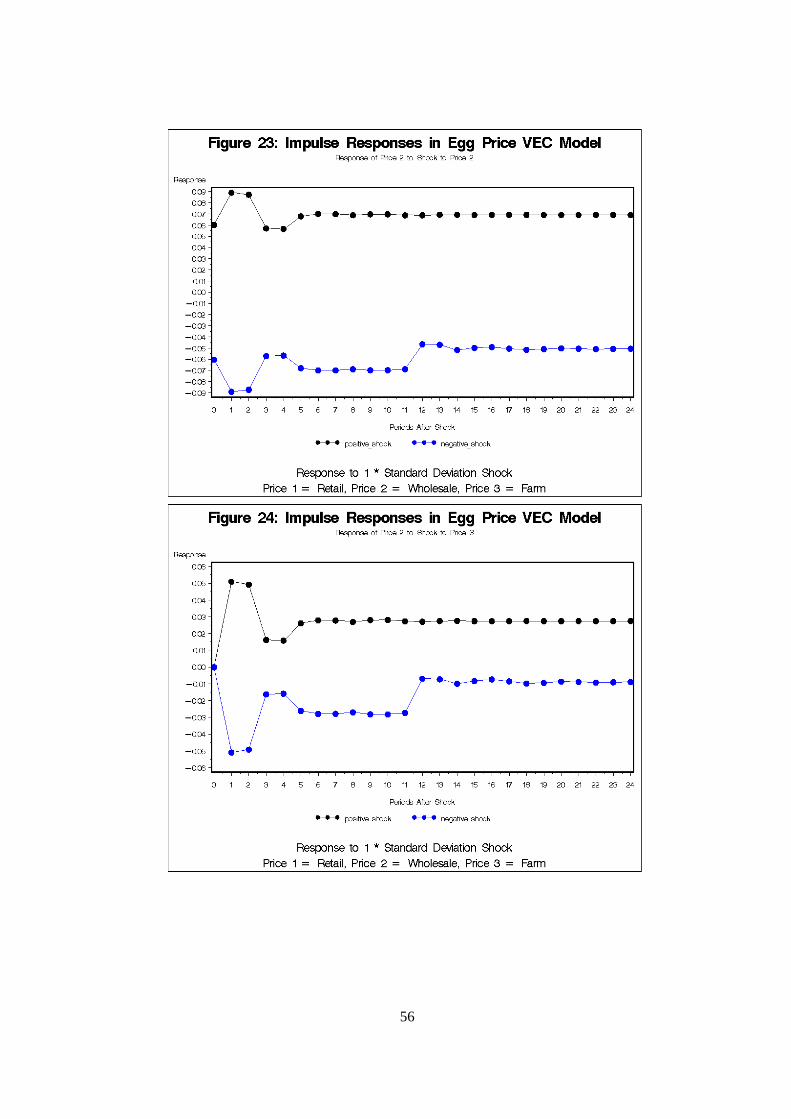
56

57

58